Relating inverse-derived basal sliding coefficients beneath ice sheets to other large-scale variables David Pollard Pennsylvania State University Robert DeConto University of Massachusetts Land Ice Working Group/CESM meeting NCAR, February 14-15 2013

Welcome message from author
This document is posted to help you gain knowledge. Please leave a comment to let me know what you think about it! Share it to your friends and learn new things together.
Transcript

Relating inverse-derived basal sliding coefficients beneath ice sheets
to other large-scale variables
David Pollard
Pennsylvania State University
Robert DeConto University of Massachusetts
Land Ice Working Group/CESM meeting NCAR, February 14-15 2013

1. Deduce basal sliding coefficients C(x,y) by simple model inversion - (like last year) 2. Don’t impose any constraints due to basal temperature or hydrology - (unlike last year) 3. Then compare C(x,y) patterns with basal temperature, melt, topography - new parameterization for C(x,y)?
Outline
4. Fails…Why?

Blue: C = 10-10 m a-1 Pa-2 Orange: C = 10-5 m a-1 Pa-2
Crude C(x,y) map: sediment if rebounded bed is below sea level, hard bedrock if above
where ub = basal ice velocity, τb = basal shear stress , N = effective pressure, Tb = basal temperature, f(Tb) = 0 if bed is frozen, 1 if bed is at melt point
• Sliding velocity depends on basal shear stress, intrinsic bed conditions, and basal hydrology or temperature:
or
ub = C(x,y) f(Tb) τbn ub = C(x,y) N-qτb
n
Common basal sliding laws in Antarctic-wide models
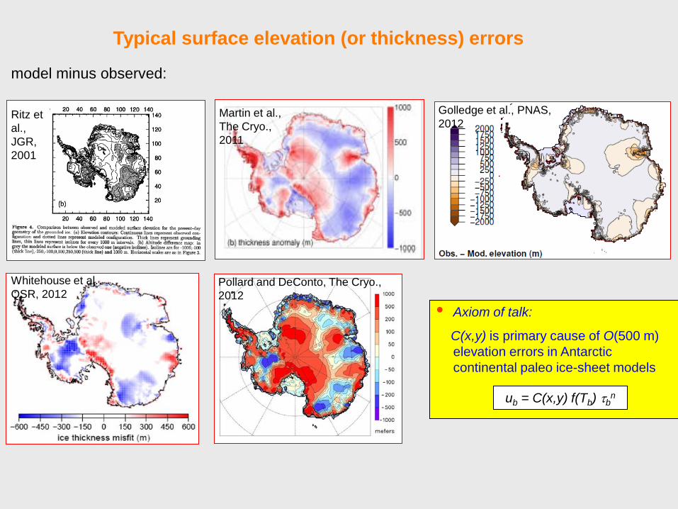
Golledge et al., PNAS, 2012
Ritz et al., JGR, 2001
Typical surface elevation (or thickness) errors
model minus observed:
Martin et al., The Cryo., 2011
Pollard and DeConto, The Cryo., 2012
Whitehouse et al. QSR, 2012
• Axiom of talk:
C(x,y) is primary cause of O(500 m) elevation errors in Antarctic continental paleo ice-sheet models
ub = C(x,y) f(Tb) τbn
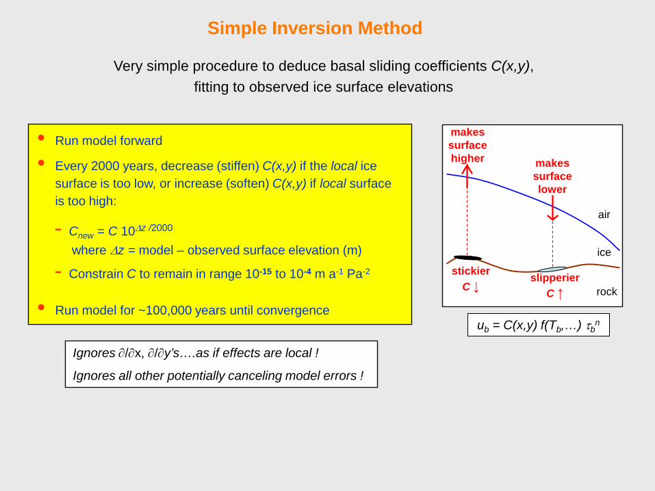
Ignores ∂/∂x, ∂/∂y’s….as if effects are local !
Ignores all other potentially canceling model errors !
• Run model forward
• Every 2000 years, decrease (stiffen) C(x,y) if the local ice surface is too low, or increase (soften) C(x,y) if local surface is too high:
• Run model for ~100,000 years until convergence
- Cnew = C 10∆z /2000 where ∆z = model – observed surface elevation (m)
- Constrain C to remain in range 10-15 to 10-4 m a-1 Pa-2
Very simple procedure to deduce basal sliding coefficients C(x,y), fitting to observed ice surface elevations
makes surface lower
slipperier C ↑
stickier C ↓
makes surface higher
air
ice
rock
Simple Inversion Method
ub = C(x,y) f(Tb,…) τbn

this talk
2 strategies in using the inverse method
Imagine that we know f(…), and apply it during the inversion procedure, to deduce C(x,y) representing intrinsic bedrock properties.
ub = C(x,y) f (Tb , hydrol., topog., … ) τb
Don’t apply f(…) during inversion. Invert for C'(x,y). Then try to find a function f so that C' =C.f , i.e., f (…) ≈ 0 in regions with C'≈0, and f =1 outside
We can write the sliding law either as or as
ub = C'(x,y) τb
(last year’s talk, and The Cryo, 2012)

Results of inverse method, no basal temperature constraint
Final elevation error Δhs
Deduced sliding
coefficients C'
log1 0 (m a-1 Pa-2)
• Purple regions are where sliding ≈ 0
• Ideally, they correspond to frozen beds, or no basal water supply
Basal temperature Tb
• But they don’t correspond to Tb< 0
r = 0.109
• Can we find a function f(Tb, topog., melt) that does?

Attempt at f(…) using basal temperature and sub-grid bed roughness
Basal temperature Tb
Sub-grid standard deviation of Bedmap2 elevations (s) f (Tb,s)
=
Bed topography (Bedmap2)
1
Tb
0
f
0
-.02 s
C' = C(x,y) f(Tb, s)
“Sub-grid valley bottoms may still be unfrozen even if Tb < 0”
×
log1 0 (m a-1 Pa-2)
Deduced sliding coefficients C'
• But resulting “f(Tb,s) ≈ 0” pattern does
not resemble purple regions C'≈ 0
• Main problem is that Tb and s both resemble large-scale bed topography
r = -0.006
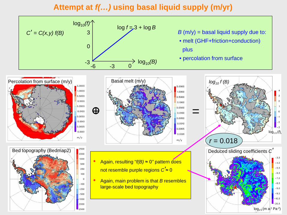
Attempt at f(…) using basal liquid supply (m/yr)
C' = C(x,y) f(B)
B (m/y) = basal liquid supply due to: • melt (GHF+friction+conduction) plus • percolation from surface
=
Basal melt (m/y)
log1 0 (f)
log10 f (B) Percolation from surface (m/y)
+
Bed topography (Bedmap2)
log10(B) -6
log10(f)
0
-3 -3 0
3 log f = 3 + log B
log1 0 (m a-1 Pa-2)
Deduced sliding coefficients C'
• Again, resulting “f(B) ≈ 0” pattern does
not resemble purple regions C'≈ 0
• Again, main problem is that B resembles large-scale bed topography
r = 0.018

Why have these attempts at f(…) failed?
1) Incorrect internal deformation (mostly SIA) - incorrect enhancement factor E ?
2) Incorrect longitudinal stress dynamics (hybrid model)
3) Basal hydrologic flow system (re-arranges B)
4) Geothermal Heat Flux distribution

Why # 1: Results of inverse method, different enhancement factors E Inverse with no basal temperature constraint on sliding
E=0.1 E=0.5 E=0.75 E=1 E=2
log1 0 (m a-1 Pa-2)
Final elevation error Δhs
Deduced sliding
coefficients C'
Basal temperature Tb
• Increasing E requires less sliding, more areas with C'≈ 0 (around EAIS flanks)
• None of the purple C'≈ 0 patterns resemble frozen-bed patterns Tb<0
• Fabric? …E(x,y,z)? …Anisotropic models?
e.g., Wang and Warner, Ann. Glac, 1999; Seddick et al., TC 2011
r = 0.109 r = 0.053 r = -0.012 r = 0.008 r = 0.160

log1 0 (m a-1 Pa-2)
Why # 2: Incorrect longitudinal-stress dynamics (hybrid model)
Deduced sliding
coefficients C'
• Many areas with C'≈ 0 (purple) are close to ice sheet margins
• Could be compensating for dynamical errors in hybrid model – too much internal shear flow near margins ?
• Test with Full Stokes models

Why # 3: Basal hydrologic flow system (re-arranges B)
• Current model lacks basal hydrology
• Basal flow could transport water supply B, and
produce patterns like purple C' > 0 regions (?)
Pattyn, EPSL, 2010
Basal melt (m/y)
Subglac. flux (103 m2 y-1)
log1 0 (m a-1 Pa-2)
Deduced sliding coefficients C'
Basal melt (m/y)
A subglacial water-flow model for West Antarctica A.M. Le Brocq, A.J. Payne, M.J. Siegert, R.B. Alley
J. Glaciol., 2009

Why # 4: Geothermal Heat Flux distribution
Geothermal heat flux (mW m-2):
two-valued (used here)
Fox Maule et al., Science, 2005
mW m-2
Shapiro and Ritzwoller, EPSL, 2004
Pattyn, EPSL, 2010
• Perhaps real GHF distribution has more structure, influencing
basal melt
• Nb: Modern Siple coast is streaming, Wilkes basin outlet is not – due to high GHF and volcanism upstream of Siple? *
* Behrendt, GPC 2004; Blankenship et al., ARS 2001; Parizek et al., GRL 2002
Ice elevations (observed)

But…regardless of basal physics…the only input to the model with fine structure are Bedmap2 elevation maps
log1 0 (m a-1 Pa-2)
Deduced sliding coefficients C'
Surface: 2hs = ∂2hs/∂x2 + ∂2hs/∂y2
Δ
• Still no clear connection
with C'≈ 0 (purple) patterns
• So where do the C'≈ 0 patterns come from in the model ?
• Do they indicate any real physical process ?
cf. Plan curvature (Le Brocq et al., GRL 2008)
r = 0.281
Bed: 2hb = ∂2hb/∂x2 + ∂2hb/∂y2
Δ
r = 0.193
Bed |slope|: √ [ (∂hb/∂x)2 + (∂hb/∂y)2 ]
r = -0.133

End
Results of inverse method, no basal temperature constraint
Final elevation error Δhs
Deduced sliding
coefficients C'
log1 0 (m a-1 Pa-2)
• Purple regions are where sliding ≈ 0
• Ideally, they correspond to frozen beds, or no basal water supply
Basal temperature, Pattyn, EPSL, 2010
Basal temperature Tb
• But they don’t correspond to Tb< 0
r = 0.109
• Can we find a function f(Tb, topog., melt) that does?

• If E is too small, nearly all motion has to be basal sliding ⇒ positive surface errors where base is frozen
• If E is too large, too much internal flow. If it exceeds the balance velocity, C inversion can’t help ⇒ large ubiquitous negative surface errors
• Best results for E ≈ 1
E = 8 E = 4
E = 2
E = 1
E = 0.5
E = 0.1
Constraining the internal-flow enhancement factor E

Inverse with no basal T effect, E=0.75 x factor 1 to 0.3 depending on distance to nearest dome
Δhs
C(x,y)
Tb
log1 0 (m a-1 Pa-2)
Results of inverse method, no Tb effect, E=0.75 x f(distance to dome)
General or review: Alley et al., 1988, Nature. Gagliardini et al., 2009, Low Temp. Sci.
E = f (τxz, τzz): Wang and Warner, 1999, Ann. Glac.
Ren et al., 2011, JGR.
E = f(z): Mangeney and Califano, 1998, JGR
Graversen et al., 2011, Clim. Dyn.
Anisotropic models: Gillet-Chaulet et al., 2005, J. Glac. (GOLF law)
Ma et al., 2010, J. Glac. → E (sheet vs. shelf).
Seddick et al., 2011, The Cryo (CAFFE model)
Fabric, anisotropy, variable enhancement coefficients:
r = 0.132

Results of inverse method, with basal temperature constraint
Final elevation error Δhs
Deduced sliding
coefficients C(x,y)
Basal temperature
Tb
• Δhs over mountain ranges is improved by dependence on s
• But not completely – hs still too high over mountains
Basal fraction
unfrozen (0 to 1)
ub = C(x,y) f(Tb. s) τbn
log1 0 (m a-1 Pa-2)
where f(Tb) = 0 for frozen bed, ramps to 1 for bed at melt point, and width of ramp increases with sub-grid bed roughness s

Plan curvature
Le Brocq et al., GRL, 2008
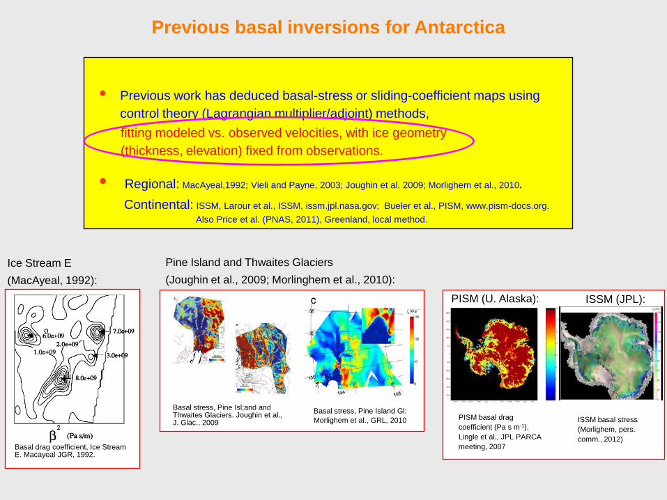
Previous basal inversions for Antarctica
• Previous work has deduced basal-stress or sliding-coefficient maps using control theory (Lagrangian multiplier/adjoint) methods,
fitting modeled vs. observed velocities, with ice geometry (thickness, elevation) fixed from observations.
• Regional: MacAyeal,1992; Vieli and Payne, 2003; Joughin et al. 2009; Morlighem et al., 2010.
Continental: ISSM, Larour et al., ISSM, issm.jpl.nasa.gov; Bueler et al., PISM, www.pism-docs.org. Also Price et al. (PNAS, 2011), Greenland, local method.
Basal drag coefficient, Ice Stream E. Macayeal JGR, 1992.
Ice Stream E (MacAyeal, 1992):
Basal stress, Pine Isl;and and Thwaites Glaciers. Joughin et al., J. Glac., 2009
Basal stress, Pine Island Gl: Morlighem et al., GRL, 2010
Pine Island and Thwaites Glaciers (Joughin et al., 2009; Morlinghem et al., 2010):
PISM basal drag coefficient (Pa s m-1). Lingle et al., JPL PARCA meeting, 2007
ISSM basal stress (Morlighem, pers. comm., 2012)
ISSM (JPL): PISM (U. Alaska):

Relating inverse-derived basal sliding coefficients beneath ice sheets
to other large-scale variables
David Pollard
Pennsylvania State University
Robert DeConto University of Massachusetts
Land Ice Working Group/CESM meeting NCAR, February 14-15 2013

Summary
• Simple inverse method “works”:
(a) converges, (b) reduces surface elevation errors, (c) deduces reasonable C(x,y) patterns.
• Independent of ice model. Just needs:
(a) run for ~200,000 years, (b) bedrock parameter(s) that make ub increase or decrease.
• BUT some of the deduced C(x,y) must be due to other model errors, not real bed conditions.
Lesser of two evils: cancelling errors vs. O(500m) biases in surface elevation
• Next steps:
- Combine with large-ensemble techniques? (Stone et al., The Cryo. 2010; Tarasov et al., EPSL, 2011)
- Apply to last deglaciation (Briggs et al., ISAES abs., 2011.; Whitehouse et al., QSR, 2012)
Related Documents