Relating 4D seismics to reservoir geomechanical changes using a discrete element approach

Geophysical Prospecting, 2010, 58, 657–668 doi: 10.1111/j.1365-2478.2009.00859.x

Relating 4D seismics to reservoir geomechanical changes usinga discrete element approach

Haitham Alassi1∗, Rune Holt2 and Martin Landrø2

1SINTEF Petroleum Research, S.P. Andersens Vei 15B, 7031 Trondheim, Norway, and 2NTNU, Department of Petroleum Engineering andApplied Geophysics, S.P. Andersens Vei 15A, 7491 Trondheim, Norway

Received March 2009, revision accepted November 2009

ABSTRACTA modified discrete element method is briefly introduced and used for modellingreservoir geomechanical response during fluid injection and depletion. The modifiedapproach works as a continuum method until some local failure is initiated, afterwhich it behaves like a discrete element method on a polygonal lattice. The methodis advantageous for modelling fracture developments in rocks. It is applied here tosynthetic models of two reservoirs taken from the North Sea (Gullfaks and Elgin-Franklin). For Gullfaks, two cases of water injection were modelled, one with lowhorizontal effective stress and the other with low vertical effective stress. Verticalfractures are developed in the first case, whereas horizontal fractures are developedin the second case. This would not have been seen using traditional methods. Basedon 4D seismics data for the Gullfaks field, one may envision that horizontal fracturescould have been formed. The Elgin-Franklin synthetic model is used to study variousscenarios of changing stress field around the depleting reservoir. Based on 4D seismicsdata from this field, one may see changes that could be interpreted in terms of possiblefault reactivation.

Key words: Modelling, Monitoring, Time lapse

INTRODUCTIO N

In recent years several examples have been presented wheregeomechanical changes within and outside hydrocarbon reser-voirs are visualized through time-lapse (4D) seismic. For ex-ample, Hatchell and Bourne (2005) showed evidence of over-burden stretching (resulting from reservoir compaction) usingtime shifts obtained from 4D seismic data. Barkved and Kris-tiansen (2005) could see shear wave splitting caused by stress-induced anisotropy above the rim of a depleting reservoir.

Stress changes directly affect properties of hydrocarbonreservoirs and surrounding rocks (e.g., Teufel, Rhett andFarrell 1991; Addis 1997; Kenter et al. 1998; Holt, Flornesand Fjær 2004), including seismic velocities. Thus, seismic

∗E-mail: [email protected]

data can be used as a tool for reservoir monitoring by har-nessing time shift and reflectivity changes in the seismic data(e.g., Landrø and Stammeijer 2004). In addition, the alter-ation of the stress regimes inside and outside hydrocarbonreservoirs might create a potential for fault reactivation (Segalland Fitzgerald 1998), which may trigger fractures leading toseismic activities. Fractures and seismic activities can also betriggered during fluid injection and used as another tool forreservoir monitoring, which is usually known as passive seis-mic monitoring (e.g., Maxwell and Urbancic 2001).

Based on the above, there is a need for numerical methodsthat are advanced enough to model geomechanical changes be-yond elasticity and yet simple enough to code and understand.Traditionally, finite element modelling has been applied, pri-marily within the frames of linear elasticity. Fault reactivationand fracture development may however be more realisticallymodelled using the discrete element method, developed by

C© 2010 European Association of Geoscientists & Engineers 657

658 H. Alassi, R. Holt and M. Landrø

Cundall and Strack (1979). This is primarily related to itsability to model fracture development and localization in adynamic manner and by its ability to deduce complex geome-chanical behaviour on the basis of simple contact behaviourat a smaller length scale.

In previous work (Alassi, Li and Holt 2006) we showed theability of using an existing discrete element method (particleflow code, e.g., Potyondy and Cundall 2004) in modellingreservoir geomechanics including fracture developments andfault reactivation. In that case, the elements were circular disks(of 40 m diameter) in 2D (spheres in 3D). A modified discreteelement approach, which is presented schematically below,has been proposed in order to deal with the same problemmore efficiently (Alassi 2008). In this paper, we will furtheruse the modified discrete element to model geomechanicalbehaviour of two North Sea reservoir cases. The first case isbased on a 2D synthetic model of the Gullfaks field wherethe effect of fluid injection will be studied. This case waspresented during the EAGE 2008 meeting (Alassi, Holt andLandrø 2008) but in this paper it will be discussed in moredetail. The second case is based on 2D sections taken fromthe Elgin-Franklin field, where the effect of depletion on faultreactivation will be studied. In both cases the results will becompared with available 4D seismic data.

RESERVOIR GEOME C H A N I C S : T H E ORYA N D BA C K G R O U N D

Analytical modelling: stress path coefficients

As the fluid pressure changes inside a subsurface compart-ment, like within a petroleum reservoir, the stresses will alsochange. Stress changes (�σ i) can be quantified through stresspath coefficients (Hettema et al. 2000) using pore pressurechange (�P), according to

γi = �σi

�P, (1)

where σ i is the total stress (i = v is vertical and i = h is hori-zontal stress).

Rudnicki (1999) derived analytical solutions for the verticaland horizontal stress path coefficients (γ v and γh) assuming anellipsoidal reservoir with linearly poroelastic properties and atlarge enough depth that it can be considered as embedded inan infinite surrounding medium with uniform pore pressurechange. For the case when the elastic properties of the reser-voir and the surroundings are equal, the stress path coefficients

inside the reservoir can be written as follows

γv = α1 − 2v

1 − v

e(1 − e2)3/2

[cos−1(e) − e(1 − e2)1/2], (2)

γh = α1 − 2v

1 − v

[1 − e

2(1 − e2)3/2(cos−1(e) − e(1 − e2)1/2)

].

(3)

Here e is the aspect ratio (e = thickness/diameter) of thedepleting or inflating reservoir zone. v is Poisson’s ratio ofthe drained rock and α is Biot’s poroelastic coefficient. Forinfinite extension and/or zero thickness reservoir (e = 0) therewill be no stress arching, γ v = 0. With increasing aspect ratioe, γ v increases and in the limit of a spheroidal reservoir zone(e = 1), γv = γh = α 1−2v

1−v(according to equations (2) and (3)).

In this paper, we will use an effective stress σ ’ defined as thenet stress or the difference between external stress and porepressure instead of the total stress σ . This is justified becausethis effective stress is used to define failure criteria. Seismicvelocity changes are also more directly related to changes ineffective stress.

A modified discrete element approach

A modified discrete element approach is proposed (Alassi2008) to model fracture developments and fault reactivationinside and outside hydrocarbon reservoirs during fluid with-drawal and injection. The advantage of the method is that itbehaves like a continuum model (e.g., finite element method)before failure and like a discontinuum model (e.g., discreteelement method) after failure.

Consider Fig. 1(a), which shows a cluster made from threeelements packed in a triangular shape. In the discrete elementmethod the constitutive relation that relates the internal forcesat the contacts to the contact relative displacements are callednormal and shear stiffness coefficients, kn and ks. For thiscluster we would like to write the internal constitutive rela-tion that relates the normal contact forces fn to the normal

Figure 1 Representation of the modified discrete element method us-ing a) spherical and b) Voronoi’s element.

C© 2010 European Association of Geoscientists & Engineers, Geophysical Prospecting, 58, 657–668

Relating 4D seismics to reservoir geomechanical changes 659

contact relative displacements un in a matrix form. The shearcontact force is also neglected by setting the contact shearstiffness ks = 0. Then the modification of the original discreteelement method is done by adding new stiffness coefficientsaij, see equation (4). Notice that the elements are not neces-sary circular, they can follow Voronoi’s shapes, which makesit easier to build more complicated models with the help ofautomatic mesh generation codes, see Fig. 1(b).

⎧⎪⎪⎪⎨⎪⎪⎪⎩

fn1

fn2

fn3

⎫⎪⎪⎪⎬⎪⎪⎪⎭

=

⎡⎢⎢⎢⎣

kn1 a12 a13

a21 kn2 a23

a31 a32 kn3

⎤⎥⎥⎥⎦

⎧⎪⎪⎨⎪⎪⎩

un1

un2

un3

⎫⎪⎪⎬⎪⎪⎭

. (4)

Furthermore, the relation between the stress σ = {σ xx σ yy

σ xy}T and the internal forces fn and the relation between thestrain ε = {εxx εyy εxy}T and the relative displacements un aregiven as

σ = 1A

MTfn, (5)

un = Mε, (6)

M is the unit normal vector matrix defined as

M =

⎡⎢⎢⎣

I211d1 I2

12d1 I11I12d1

I221d2 I2

22d2 I21I22d2

I231d3 I2

32d3 I31I32d3

⎤⎥⎥⎦ , (7)

where Im1 = cosθm and Im2 = sinθm and the angle θm repre-sents the normal vector orientation of the contact m inside thecluster. dm is the contact’s length (the distance between thetwo elements that are in contact). A is the area of the cluster(or triangle).

Equations (5) and (6) will make it easy to define failure cri-teria, since the criteria are usually given as a function of stressand strain. Remember also that the stress can be related to thestrain by using material conventional constitutive matrix C as

σ = Cε. (8)

So it is now possible to relate the internal constitutive matrixK, see equation (4) and the material conventional constitutivematrix C to each other by using equations (4)–(8) as follows:

C = 1A

MTKM. (9)

After K has been retrieved equation (9), the solution schemewill be similar to the regular discrete element method. In

this method the contact forces are updated incrementally, thismeans (dfn = K dun) and fn

new = fn+dfn, where dun at eachcontact is calculated by using the elements’ velocities vi andthe time step dt as follows

dun = (Element1 − (vi )Element2

)Ii dt = �vi Ii dt, (10)

then the forces are applied to each element and Newton’ssecond law is used to update the elements’ motion, see Cundalland Strack (1979) for more details.

For a failing cluster, both kn and ks are used to update thenormal and the shear forces at each contact and thus a shearcontact force fs will start to build up in this cluster and at eachcontact according to dfs = ks dus, where dus is calculated as

dus = |�vi − �v j Ij Ii |dt. (11)

This means that ks will be zero before failure but will have afinite value after failure to model the shear stress that is devel-oped at the cracks’ interfaces. The new stiffness coefficient aij

introduced in equation (4) is deleted at this stage and contactseparation is allowed, which will weaken the failing clusterand cause the stress to redistribute. Stress redistribution willbe responsible for fracture propagation into the surroundingclusters as the stresses in these clusters reach the threshold. Ineach failing cluster the contact that has its plane close to theperpendicular of the minimum stress will open first, thus crackdirection and opening are modelled automatically without theneed to know the minimum stress direction.

The main difference between this approach and the regu-lar discrete element method is that the material can behaveaccording to a continuum model before failure where con-ventional elastic properties can be given to the material basedon equation (9), while the material behaves according to aregular discrete element method after failure.

RESERVOIR GEOMECHANICAL RESPO NSETO FLUID INJECTION

In this section, the geomechanical behaviour of hydrocarbonreservoirs during fluid injection will be studied using the ana-lytical approach as well as the modified discrete element ap-proach sketched above.

Using the effective stress as σ ′i = σi − P (P is the pore pres-

sure) and since tensile failure is expected when the final effec-tive stress becomes more tensile than the rock tensile strengthT0, one finds that in a normal fault regime (vertical stress isthe maximum principal stress), vertical fractures will develop

C© 2010 European Association of Geoscientists & Engineers, Geophysical Prospecting, 58, 657–668

660 H. Alassi, R. Holt and M. Landrø

if the pore pressure increase �P exceeds:

�P ≥ �Pcrit,vert = σ ′h,ini + T0

(1 − γh). (12)

When the pore pressure is increased, the vertical stress willat some stage become the minor principal stress. In such acase, horizontal tensile fractures are expected, provided:

�P ≥ �Pcrit,hor = σ ′v,ini + T0

(1 − γv). (13)

The initiation pressure for horizontal fractures may in cer-tain cases be lower than for vertical fractures. Please note thatthere is limited field evidence for such behaviour, as pointedout by, e.g., Santarelli, Havmøller and Naumann (2008). Thereason for this may be that the stress path of a reservoir duringinjection is different from that during initial depletion. How-ever, in particular, in cases of thermally assisted injection,principal stress orientation changes have been documented(Dusseault and Simmons 1982). It remains a topic of furtherresearch to evaluate under what conditions this may or maynot happen in the field.

A NU M E R I C A L T E S T

To test the modified discrete element approach against theabove analytical solution, an elliptical 2D reservoir with di-mension (2000 × 200 m2) is built, the model boundaries arefixed and a uniform effective stress is installed without grav-ity effect. Such a technique for installing the initial and theboundary conditions is adopted throughout this paper. Thereservoir has the following elastic properties, Young modulusE = 10 GPa and Poisson’s ratio ν = 0.3. The initial verticaleffective stress is chosen as 12 MPa and the initial horizontaleffective stress is chosen as 4.5 MPa, the tensile strength forthe reservoir is set to 0.5 MPa. The fluid injection is simulatedby increasing the pore pressure uniformly and gradually insidethe reservoir up to �P = 11 MPa. If one uses equations (2), (3)and (12) (with the given aspect ratio e = 0.1), it will be easy toshow that vertical fractures should develop. The result of thesimulation is shown in Fig. 2, where the development of ver-tical fractures is seen (as predicted by the analytical solution).The intensity of the fractures increases towards the edges. Infact, the fractures start at the edges and then move towardsthe reservoir centre. This is a result of the stress concentrationnear the edge of the reservoir.

Figure 2 also shows the horizontal and vertical effectivestresses after injection. The horizontal effective stress (middle)

Figure 2 Vertical fractures developed inside elliptical reservoir andthe effective stress distribution as a result of uniform pressure increaseusing the modified discrete element approach, ν = 0.3.

varies between 0–1 MPa throughout the reservoir except inthe middle where it is slightly negative (tension) and also nearthe left edge of the reservoir. The latter might be a modelartefact, because the reservoir is heavily fractured there. Thevertical effective stress (bottom) remains above zero inside thereservoir. An interesting thing to be noticed is that the verticalfractures tend to separate the reservoir into compartments,this can be seen by looking to the vertical effective stress inthe overburden where the stress concentration just above thereservoir can be considered as local arching usually seen atcompartment (or reservoir) edges.

2D SYNTHETIC M ODEL BASEDON GULLFAKS F IELD

In this section we will test our method on a synthetic modelof the Gullfaks field in the North Sea. The study will howeverbe limited to two dimensions (2D) only. In previous works(Kvam and Landrø 2005; Duffaut and Landrø 2007) effortswere made to detect pore pressure increase inside the Gullfaksfield by acquired time-lapse data. We will extend their workby performing geomechanical modelling together with fluidcoupling to see if fractures can initiate and where and howthey may propagate. We use a finite difference scheme for fluidflow simulation, where the spatial discretization is achievedthrough a network of pipes and each pipe matches a contactin the modified discrete element method. Notice that flow

C© 2010 European Association of Geoscientists & Engineers, Geophysical Prospecting, 58, 657–668

Relating 4D seismics to reservoir geomechanical changes 661

Figure 3 Gullfaks 2D synthetic model used for geomechanical mod-elling.

Table 1 Properties of the Gullfaks 2D synthetic model (Duffaut et al.2007). The horizontal well information is provided by StatoilHydro

Properties Values

Initial horizontal effective stress σ ′h,ini 4.5 MPa

Initial vertical effective stress σ ′v,ini 8.0 MPa

Pore pressure change �P 7.0 MPaReservoir length 1250 mReservoir depth 2036 mReservoir thickness 120 mHorizontal well length 300 mYoung’s Modulus E 10 GPaPoisson’s ratio ν 0.25Tensile strength T0 0.50 MPa

through induced fractures is not modelled at this stage andthus permeability remains unchanged during the modelling,this will simplify the modelling but will induce error at thesame time. However, a simple extension can be used to solvethis in which the permeability of each pipe that correspondsto a fracture is changed, see Alassi (2008) for more details.

The Gullfaks 2D synthetic model is shown in Fig. 3. Ten-sile strength, Young’s modulus and Poisson’s ratio are chosensomewhat arbitrarily; Table 1 shows the selected data.

The injection strategy of the Gullfaks field is that the injec-tors are normally placed in the northern part of the field andwater is injected below the original oil-water contact. Apartfrom some scarce examples of gas injection, the majority ofthe injectors are water injectors, all operating with the samepurpose: increasing the pressure in selected formations as thefield is depleted.

We start by modelling a reference case where the data inTable 1 are used. The modelling begins by increasing the well

pressure (�P) by 7 MPa. The resulting horizontal and verticaleffective stresses at two stages, at the middle and the end, areshown in Fig. 4. Notice that the effective stresses are abovezero (still compressive) and thus no fractures are developed.

However, because no fractures developed in the referencecase, we decided to make a sensitivity study by fixing all fac-tors except the effective stresses. Two cases will be studiedin the following two subsections, one with lower horizontaleffective stress (σ ′

h,ini = 3 MPa vs. 4.5 MPa as the referencelevel) and the other with lower vertical effective stress (σ ′

v,ini =6.5 MPa vs. 8.0 MPa as the reference level).

The new values of σ ′h,ini and σ ′

v,ini are not chosen arbitrarily.In fact, by looking to equations (12) and (13) and using thereservoir aspect ratio e ≈ 0.1 (from Table 1) and knowingthat �P = 7 MPa, one can calculate the critical values of thehorizontal and vertical effective stresses that result in creatingfractures. In our case we got the following values σ ′

h,ini ≈2.2 MPa and σ ′

v,ini ≈ 6 MPa. So we decided to choose slightlyhigher values for the initial effective stresses in the numericalmodel than these calculated ones.

Case 1, low horizontal effective stress (σ ′h,ini = 3 MPa)

The initial vertical effective stress is taken from Table 1, i.e.,σ ′

v,ini = 8.0 MPa, while the initial horizontal effective stress ischanged to 3.0 MPa. We then start the modelling by increas-ing the well pressure by 7 MPa and the model is monitored forfracture development. Notice that one-way coupling is usedfrom the fluid model to the geomechanical model. Figure 5shows the development of fractures together with the pres-sure change distribution at several stages of the modelling.As shown, at the early stage the fractures start near the welledges, then they propagate vertically. On the other hand, atthe end of the modelling when the pore pressure stabilizes,vertical fractures develop at the reservoir edges.

The analytical solution described in the previous sectionshows that no vertical fractures should develop in this case(i.e., the condition of σ ′

h,ini ≤ 2.2 MPa is to be met for verticalfractures to develop). The reason why fractures are developedin the numerical model is due to the fluid injection well, whereas the well pressure increases stress concentrates (more ten-sion) at the well tips, resulting in vertical fractures. The waythe pressure front moves from the horizontal well also affectshow the fractures propagate. Finally, vertical fracture devel-opment at the reservoir edges and at the end of the simulation(when the pressure stabilizes) is due to the stress concentra-tion at those edges. Such behaviour is not predicted by theanalytical model because it assumes elliptical geometry with

C© 2010 European Association of Geoscientists & Engineers, Geophysical Prospecting, 58, 657–668

662 H. Alassi, R. Holt and M. Landrø

Figure 4 Pressure change distribution and effective stresses as a result of fluid injection for the reference case, no fractures developed.

Figure 5 Fractures development (left) and pressure change distribution (right) at four stages during fluid injection, Case 1. Notice that thefractures develop vertically.

no sharp corners. Further, incorporating fluid coupling gives aheterogeneous pore pressure distribution inside the reservoir,contrary to the homogeneous pressure field assumed in theanalytical model.

Case 2, low vertical effective stress (σ ′v,ini = 6.5 MPa)

The initial horizontal effective stress is taken from Table 1,i.e., σ ′

h,ini = 4.5 MPa, while the initial vertical effective stress

is changed to 6.5 MPa. In this case and after the modelling isstarted by fluid injection, the fractures start to develop at thewell edges and they propagate horizontally toward the reser-voir edges. At late stages of the modelling (when the pressurestabilizes), the fractures initiate at the edges of the reservoirand then they propagate horizontally toward the reservoircentre, see Fig. 6. In other words, horizontal fractures are de-veloped even though the initial normal effective stress is largerthan the horizontal one. This can be explained by equations

C© 2010 European Association of Geoscientists & Engineers, Geophysical Prospecting, 58, 657–668

Relating 4D seismics to reservoir geomechanical changes 663

Figure 6 Fractures development (left) and pressure change distribution (right) at four stages during fluid injection, Case 2. Notice that thefractures develop horizontally.

(12) and (13), where in certain conditions the reduction in σ ′v

becomes larger than σ ′h, which means σ ′

v may reach fracturelimit before σ ′

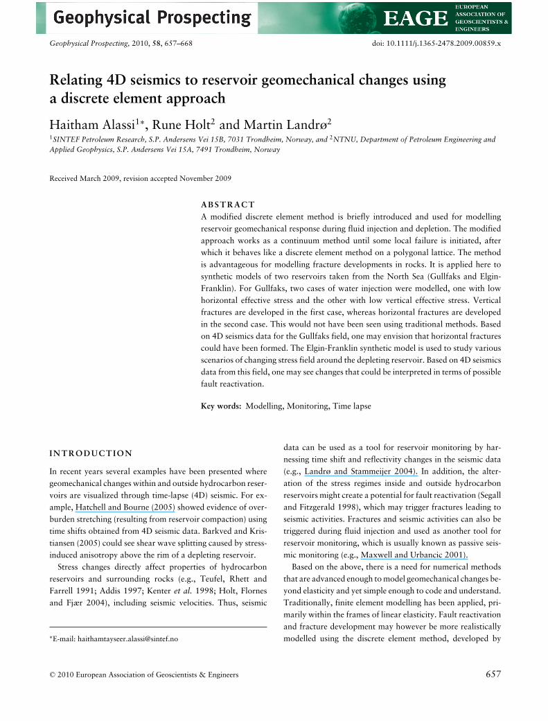
h.Figure 7 shows the vertical and horizontal effective stress

distribution for both cases at the final stage. Notice how forCase 2 the vertical effective stress becomes less than the hori-zontal one and it more or less stays around zero.

A C OMPARISON T O GULLFA K S4 D S E I S M I C S D A T A

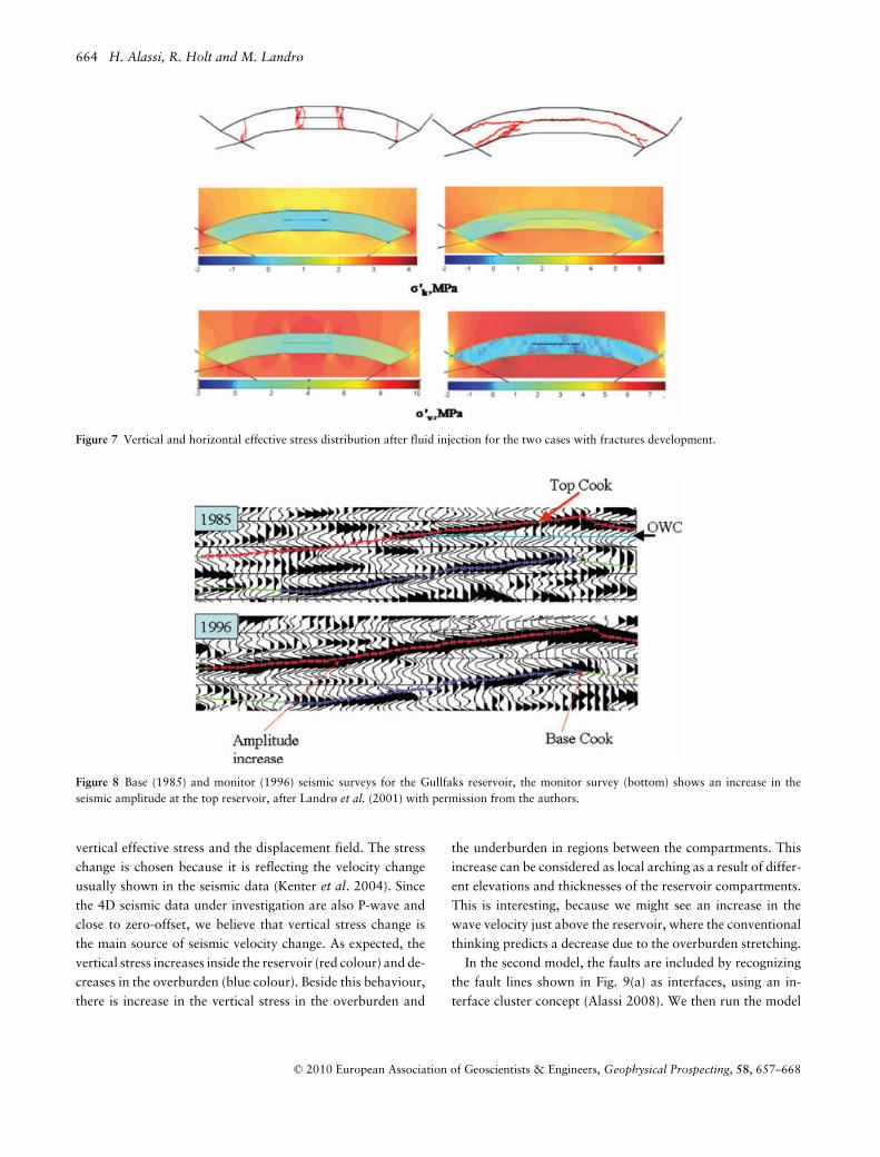
Figure 8 shows a seismic cross-section for the Gullfaks reser-voir, the base survey was acquired in 1985 and the monitorwas acquired in 1996. According to Landrø, Digranes andStrønen (2001), the increase of the seismic amplitude at topreservoir (top Cook) and the pull-down effect at bottom reser-voir (base Cook) is due to pressure increase inside the reser-voir, which resulted in a decrease in the effective stress withan associated decrease in the wave velocity. Both fracture ini-tiation scenarios predicted by our model and in particular thehorizontal fracture case, can cause such a decrease in the wavevelocity. This may be considered as a complementary possibleinterpretation but needs further evaluation before any conclu-sion can be drawn.

It is worthwhile mentioning, before finishing this section,that in the previous two scenarios, the reservoir is initiallyassumed to be like one continuum unit without interfaces orplanes of weakness. However, real reservoirs usually contain

initial fractures and small faults, which are embedded in theirbodies. In this case, stress concentrations are expected aroundthe faults, which result in fracture development, even thoughthe initial effective stress is relatively high. Such a scenario caneasily be modelled using this technique, as illustrated in thenext example.

REACTIVATIONS OF FAULTS PASS INGT H R O U G H R E S E R V O I R S D U R I N GDEPLETION: ELGIN-FRANKLIN FIELD

A single reservoir is usually separated by faults into severalcompartments. These compartments might not be aligned,having different elevations and thicknesses. Such a conditionwill enhance fault reactivation if the pore pressure reductionis large enough. Fault reactivation might be detected using 4Dseismic (Røste, Landrø and Hatchell 2007). In this section,we will perform geomechanical modelling on two 2D cross-sections taken from the Elgin-Franklin sandstone reservoir inthe North Sea. The sections are shown in Fig. 9; notice thefaults and the compartments.

Section 1

We start by installing initial stresses, then the reservoir is de-pleted by 30 MPa, neglecting the existence of the faults, i.e.,the faults are not allowed to slide. The outcome of the simula-tion is shown in Fig. 10(a). The figure depicts the change in the

C© 2010 European Association of Geoscientists & Engineers, Geophysical Prospecting, 58, 657–668

664 H. Alassi, R. Holt and M. Landrø

Figure 7 Vertical and horizontal effective stress distribution after fluid injection for the two cases with fractures development.

Figure 8 Base (1985) and monitor (1996) seismic surveys for the Gullfaks reservoir, the monitor survey (bottom) shows an increase in theseismic amplitude at the top reservoir, after Landrø et al. (2001) with permission from the authors.

vertical effective stress and the displacement field. The stresschange is chosen because it is reflecting the velocity changeusually shown in the seismic data (Kenter et al. 2004). Sincethe 4D seismic data under investigation are also P-wave andclose to zero-offset, we believe that vertical stress change isthe main source of seismic velocity change. As expected, thevertical stress increases inside the reservoir (red colour) and de-creases in the overburden (blue colour). Beside this behaviour,there is increase in the vertical stress in the overburden and

the underburden in regions between the compartments. Thisincrease can be considered as local arching as a result of differ-ent elevations and thicknesses of the reservoir compartments.This is interesting, because we might see an increase in thewave velocity just above the reservoir, where the conventionalthinking predicts a decrease due to the overburden stretching.

In the second model, the faults are included by recognizingthe fault lines shown in Fig. 9(a) as interfaces, using an in-terface cluster concept (Alassi 2008). We then run the model

C© 2010 European Association of Geoscientists & Engineers, Geophysical Prospecting, 58, 657–668

Relating 4D seismics to reservoir geomechanical changes 665

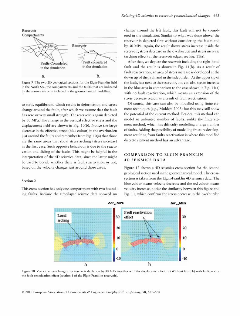
Figure 9 The two 2D geological sections for the Elgin-Franklin fieldin the North Sea, the compartments and the faults that are indicatedby the arrows are only included in the goemechanical modelling.

to static equilibrium, which results in deformation and stresschange around the fault, after which we assume that the faulthas zero or very small strength. The reservoir is again depletedby 30 MPa. The change in the vertical effective stress and thedisplacement field are shown in Fig. 10(b). Notice the largedecrease in the effective stress (blue colour) in the overburdenjust around the faults and remember from Fig. 10(a) that thoseare the same areas that show stress arching (stress increase)in the first case. Such opposite behaviour is due to the reacti-vation and sliding of the faults. This might be helpful in theinterpretation of the 4D seismics data, since the latter mightbe used to decide whether there is fault reactivation or not,based on the velocity changes just around those areas.

Section 2

This cross-section has only one compartment with two bound-ing faults. Because the time-lapse seismic data showed no

change around the left fault, this fault will not be consid-ered in the simulation. Similar to what was done above, thereservoir is depleted first without considering the faults andby 30 MPa. Again, the result shows stress increase inside thereservoir, stress decrease in the overburden and stress increase(arching effect) at the reservoir edges, see Fig. 11(a).

After that, we deplete the reservoir including the right-handfault and the result is shown in Fig. 11(b). As a result offault reactivation, an area of stress increase is developed at thedown tip of the fault and in the sideburden. At the upper tip ofthe fault, just next to the reservoir, one can also see an increasein the blue area in comparison to the case shown in Fig. 11(a)with no fault reactivation, which means an extension of thestress decrease region as a result of fault reactivation.

Of course, this case can also be modelled using finite ele-ment techniques (e.g., Mulders 2003) but this may still showthe potential of the current method. Besides, this method canmodel an unlimited number of faults, unlike the finite ele-ment method, which has difficulty modelling a large numberof faults. Adding the possibility of modelling fracture develop-ment resulting from faults reactivation is where this modifieddiscrete element method has an advantage.

COMPARISON T O ELGIN-FRANKLIN4 D S E I S M I C S D A T A

Figure 12 shows a 4D seismics cross-section for the secondgeological section used in the geomechanical model. The cross-section is taken from the Elgin-Franklin 4D seismics data. Theblue colour means velocity decrease and the red colour meansvelocity increase, notice the similarity between this figure andFig. 11, which confirms the stress decrease in the overburden

Figure 10 Vertical stress change after reservoir depletion by 30 MPa together with the displacement field. a) Without fault, b) with fault, noticethe fault reactivation effect (section 1 of the Elgin-Franklin reservoir).

C© 2010 European Association of Geoscientists & Engineers, Geophysical Prospecting, 58, 657–668

666 H. Alassi, R. Holt and M. Landrø

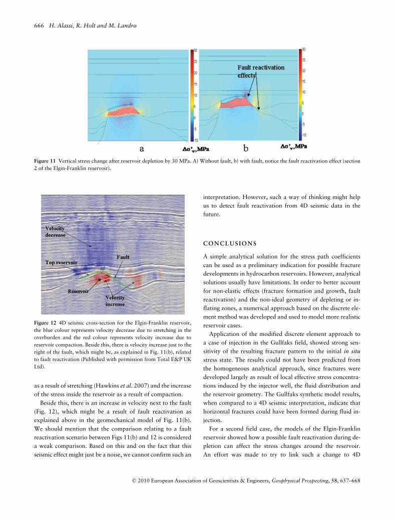
Figure 11 Vertical stress change after reservoir depletion by 30 MPa. A) Without fault, b) with fault, notice the fault reactivation effect (section2 of the Elgin-Franklin reservoir).

Figure 12 4D seismic cross-section for the Elgin-Franklin reservoir,the blue colour represents velocity decrease due to stretching in theoverburden and the red colour represents velocity increase due toreservoir compaction. Beside this, there is velocity increase just to theright of the fault, which might be, as explained in Fig. 11(b), relatedto fault reactivation (Published with permission from Total E&P UKLtd).

as a result of stretching (Hawkins et al. 2007) and the increaseof the stress inside the reservoir as a result of compaction.

Beside this, there is an increase in velocity next to the fault(Fig. 12), which might be a result of fault reactivation asexplained above in the geomechanical model of Fig. 11(b).We should mention that the comparison relating to a faultreactivation scenario between Figs 11(b) and 12 is considereda weak comparison. Based on this and on the fact that thisseismic effect might just be a noise, we cannot confirm such an

interpretation. However, such a way of thinking might helpus to detect fault reactivation from 4D seismic data in thefuture.

CONCLUSIONS

A simple analytical solution for the stress path coefficientscan be used as a preliminary indication for possible fracturedevelopments in hydrocarbon reservoirs. However, analyticalsolutions usually have limitations. In order to better accountfor non-elastic effects (fracture formation and growth, faultreactivation) and the non-ideal geometry of depleting or in-flating zones, a numerical approach based on the discrete ele-ment method was developed and used to model more realisticreservoir cases.

Application of the modified discrete element approach toa case of injection in the Gullfaks field, showed strong sen-sitivity of the resulting fracture pattern to the initial in situstress state. The results could not have been predicted fromthe homogeneous analytical approach, since fractures weredeveloped largely as result of local effective stress concentra-tions induced by the injector well, the fluid distribution andthe reservoir geometry. The Gullfaks synthetic model results,when compared to a 4D seismic interpretation, indicate thathorizontal fractures could have been formed during fluid in-jection.

For a second field case, the models of the Elgin-Franklinreservoir showed how a possible fault reactivation during de-pletion can affect the stress changes around the reservoir.An effort was made to try to link such a change to 4D

C© 2010 European Association of Geoscientists & Engineers, Geophysical Prospecting, 58, 657–668

Relating 4D seismics to reservoir geomechanical changes 667

seismic data from the reservoir based on some observationson these seismic data. To what extent this seismic anomalymay correspond to fault reactivation remains unknown, sincethis anomaly might be just a noise, however such an interpre-tation may help us in the future when more 4D seismic dataare available.

It should be mentioned that the use of this modified discreteelement approach enables us to model fault and fractures ina dynamic and easy way, which is considered an essence ofthis method. Besides, the full potential of this method remainsto be seen when large and more realistic 3D models are built,containing complex pre-existing fault patterns with expectedfracture developments.

ACKNOWLEDGE ME N T S

The authors acknowledge the Norwegian Research Coun-cil for financial support of this work through the StrategicUniversity Program ‘ROSE – Improved Overburden Charac-terization combining Seismic and Rock Physics’ at NTNU(Norwegian University of Science and Technology). The au-thors would also like to thank SINTEF Petroleum for bothits technical and financial support. This includes giving usthe time to write this contribution. A special thanks to JohnWilliams from StatoilHydro for providing valuable informa-tion about Gullfaks field. Maurice Dusseault, Cor J. Kenterand Frederic Santarelli are acknowledged for valuable andstimulating discussions. We would also like to thank TotalE&P UK Ltd (Aberdeen) and people at the GRC for their col-laboration and for allowing us to include some of the dataabout the Elgin-Franklin reservoir in this work.

REFERENCES

Addis M.A. 1997. The stress-depletion response of reservoirs. SPE38720.

Alassi H.T. 2008. Modelling reservoir geomechanics using discreteelement method: Application to reservoir monitoring. PhD thesis,NTNU, Norway.

Alassi H.T., Holt R.M. and Landrø M. 2008. Modelling reservoirgeomechanical changes caused by fluid injection–A discrete elementapproach. 70th EAGE meeting, Rome, Italy, Expanded Abstracts,E032.

Alassi H.T., Li L. and Holt R.M. 2006. Discrete element modeling ofstress and strain evolution within and outside a depleting reservoir.Pure and Applied Geophysics 163, 1–21.

Barkved O. and Kristiansen T.G. 2005. Seismic time-lapse effects andstress changes: Example from a compacting reservoir. The LeadingEdge 24, 1244–1248.

Cundall P.A. and Strack O.D.L. 1979. A discrete numeri-cal model for granular assemblies. Geotechnique 29, 47–65.

Duffaut K. and Landrø M. 2007. Vp/Vs ratio versus differen-tial stress and rock consolidation – A comparison betweenrock models and time-lapse AVO data. Geophysics 72, C81–C94.

Dusseault M.B. and Simmons J.V. 1982. Injection-induced stress andfracture orientation changes. Canadian Geotechnical Journal 19,483–493.

Hatchell P. and Bourne S. 2005. Rocks under strain: Strain-inducedtime-lapse time shifts are observed for depleting reservoirs. TheLeading Edge 24, 1222–1225.

Hawkins P.J., Howe S., Hollingworth S., Conroy G., Ben-Brahim L.,Tindle C. et al. 2007. Production-induced stresses from time-lapsetime shifts: A geomechanics case study from Franklin and Elginfields. The Leading Edge 26, 655–662.

Hettema M.H.H., Schutjens P.M.T.M., Verboom B.J.M. and Gussin-klo H.J. 2000. Production-induced compaction of a sandstonereservoir: The strong influence of stress path. SPE Reservoir Eval-uation Engineering 3, 342–347.

Holt R.M., Flornes O., Li L. and Fjær E. 2004. Consequencesof depletion-induced stress changes on reservoir compactionand recovery. Proceedings of the Gulf Rocks’04, Ppr. 04–589.ARMA/NARMS.

Kenter C.J., Beukel A.V.D., Hatchell P., Maron K. and MolenaarM. 2004. Evaluation of reservoir characteristics from timeshifts inthe overburden. Proceedings of the Gulf Rocks’04, Ppr. 04–627.ARMA/NARMS.

Kvam Ø. and Landrø M. 2005. Pore-pressure detection sensitiv-ities tested with time-lapse seismic data. Geophysics 70, O39–O50.

Landrø M. 2001. Discrimination between pressure and fluid sat-uration changes from time-lapse seismic data. Geophysics 66,836–844.

Landrø M., Digranes P. and Strønen L.K. 2001. Mapping reservoirpressure and saturation changes using seismic methods-possibilitiesand limitations. First Break 19, 12.

Landrø M. and Stammeijer J. 2004. Quantitative estimation of com-paction and velocity changes using 4D impedence and traveltimechanges. Geophysics 69, 949–957.

Maxwell S.C. and Urbancic T. 2001. The role of passive microseismicmonitoring in the instrumented oil field. The Leading Edge 19,636–639.

Mulders F.M.M. 2003. Modelling of stress development and fault slipin and around a producing gas reservoir. PhD thesis, TU Delft, theNetherlands.

Potyondy D.O. and Cundall P.A. 2004. A bonded particle model forrock. International Journal of Rock Mechanics and Mining Sciences41, 1329–1364.

Røste T., Landrø M. and Hatchell P. 2007. Monitoring overbur-den layer changes and fault movements from time-lapse seismicdata on the Valhall Field. Geophysical Journal International 170,1100–1118.

Rudnicki J.W. 1999. Alteration of regional stress by reservoirs andother inhomogeneities: Stabilizing or destabilizing? In: Proceedings

C© 2010 European Association of Geoscientists & Engineers, Geophysical Prospecting, 58, 657–668

668 H. Alassi, R. Holt and M. Landrø

of the International Congress on Rock Mechanics (eds G. Vouilleand P. Berest), pp. 1629–1637. ISRM.

Santarelli F., Havmøller O. and Naumann M. 2008. Geomechanicalaspects of 15 years water injection on a field complex: An analysisof the past to plan the future. SPE112944.

Segall P. and Fitzgerald S.D. 1998. A note on induced stress changes

in hydrocarbon and geothermal reservoirs. Tectonophysics 289,117–128.

Teufel L.W., Rhett D.W. and Farrell H.E. 1991. Effect of reservoir de-pletion and pore pressure drawdown on in situ stress and deforma-tion in the Ekofisk field. In: Rock Mechanics as a MultidisciplinaryScience (ed. J.C. Roegiers), pp. 63–72. A.A. Balkema.

C© 2010 European Association of Geoscientists & Engineers, Geophysical Prospecting, 58, 657–668