Reinforcement Learning with Fast Stabilization in Linear Dynamical Systems Sahin Lale Kamyar Azizzadenesheli Babak Hassibi Anima Anandkumar Caltech Purdue University Caltech Caltech Abstract In this work, we study model-based rein- forcement learning (RL) in unknown stabiliz- able linear dynamical systems. When learn- ing a dynamical system, one needs to stabi- lize the unknown dynamics in order to avoid system blow-ups. We propose an algorithm that certifies fast stabilization of the underly- ing system by effectively exploring the envi- ronment with an improved exploration strat- egy. We show that the proposed algorithm attains ˜ O( √ T ) regret after T time steps of agent-environment interaction. We also show that the regret of the proposed algorithm has only a polynomial dependence in the problem dimensions, which gives an exponential im- provement over the prior methods. Our im- proved exploration method is simple, yet effi- cient, and it combines a sophisticated explo- ration policy in RL with an isotropic explo- ration strategy to achieve fast stabilization and improved regret. We empirically demon- strate that the proposed algorithm outper- forms other popular methods in several adap- tive control tasks. 1 INTRODUCTION We study the problem of reinforcement learning (RL) in linear dynamical systems, in particular in linear quadratic regulators (LQR). LQR is the canonical set- ting for linear dynamical systems with quadratic reg- ulatory costs and observable state evolution. For a known LQR model, the optimal control policy is given by a stabilizing linear state feedback controller (Bert- sekas, 1995). When the underlying model is unknown, Proceedings of the 25 th International Conference on Artifi- cial Intelligence and Statistics (AISTATS) 2022, Valencia, Spain. PMLR: Volume 151. Copyright 2022 by the au- thor(s). the learning agent needs to learn the dynamics in or- der to (1) stabilize the system and (2) find the optimal control policy. This online control task is one of the core challenges in RL and control theory. Learning LQR models from scratch: The ulti- mate goal in online control is to design learning agents that can autonomously adapt to the unknown environ- ment with minimal information and also enjoy finite- time stability and performance guarantees. This prob- lem has sparked a flurry of research interest in the control and RL communities. However, there are only a few approaches that provide a complete treatment of the problem and strive for learning from scratch with no initial model estimates (Abbasi-Yadkori and Szepesvári, 2011; Abeille and Lazaric, 2018; Chen and Hazan, 2020). Other than these, the prior works focus either on the problem of finding a stabilizing policy while ignoring the control costs (Faradonbeh et al., 2018a), or on achieving low control costs while assum- ing access to an initial stabilizing controller (Abeille and Lazaric, 2020; Simchowitz and Foster, 2020). Lack of stabilization and its consequences: The existing works (Abbasi-Yadkori and Szepesvári, 2011; Abeille and Lazaric, 2017, 2018) that learn from scratch in LQRs aim to minimize the regret, which is the additional cumulative control cost of an agent com- pared to the expected cumulative cost of the optimal policy. These algorithms suffer from regret that has an exponential dependence in the LQR dimensions since they do not assume access to an initial stabilizing pol- icy. They also face system blow-ups due to unstable system dynamics. Besides poor regret performance, the uncontrolled dynamics prevent the deployment of these learning algorithms in practice. Joint goals of fast stabilization and low regret: In this paper, we design an RL agent for online LQRs that achieves low regret and fast stabilization. To de- sign stabilizing policies without prior knowledge, the agent needs to effectively explore the environment and estimate the system dynamics. However, in order to achieve low regret, the agent should also strategically exploit the gathered knowledge. Thus, the agent re-

Welcome message from author
This document is posted to help you gain knowledge. Please leave a comment to let me know what you think about it! Share it to your friends and learn new things together.
Transcript

Reinforcement Learning with Fast Stabilizationin Linear Dynamical Systems
Sahin Lale Kamyar Azizzadenesheli Babak Hassibi Anima AnandkumarCaltech Purdue University Caltech Caltech
Abstract
In this work, we study model-based rein-forcement learning (RL) in unknown stabiliz-able linear dynamical systems. When learn-ing a dynamical system, one needs to stabi-lize the unknown dynamics in order to avoidsystem blow-ups. We propose an algorithmthat certifies fast stabilization of the underly-ing system by effectively exploring the envi-ronment with an improved exploration strat-egy. We show that the proposed algorithmattains O(
√T ) regret after T time steps of
agent-environment interaction. We also showthat the regret of the proposed algorithm hasonly a polynomial dependence in the problemdimensions, which gives an exponential im-provement over the prior methods. Our im-proved exploration method is simple, yet effi-cient, and it combines a sophisticated explo-ration policy in RL with an isotropic explo-ration strategy to achieve fast stabilizationand improved regret. We empirically demon-strate that the proposed algorithm outper-forms other popular methods in several adap-tive control tasks.
1 INTRODUCTION
We study the problem of reinforcement learning (RL)in linear dynamical systems, in particular in linearquadratic regulators (LQR). LQR is the canonical set-ting for linear dynamical systems with quadratic reg-ulatory costs and observable state evolution. For aknown LQR model, the optimal control policy is givenby a stabilizing linear state feedback controller (Bert-sekas, 1995). When the underlying model is unknown,
Proceedings of the 25th International Conference on Artifi-cial Intelligence and Statistics (AISTATS) 2022, Valencia,Spain. PMLR: Volume 151. Copyright 2022 by the au-thor(s).
the learning agent needs to learn the dynamics in or-der to (1) stabilize the system and (2) find the optimalcontrol policy. This online control task is one of thecore challenges in RL and control theory.
Learning LQR models from scratch: The ulti-mate goal in online control is to design learning agentsthat can autonomously adapt to the unknown environ-ment with minimal information and also enjoy finite-time stability and performance guarantees. This prob-lem has sparked a flurry of research interest in thecontrol and RL communities. However, there are onlya few approaches that provide a complete treatmentof the problem and strive for learning from scratchwith no initial model estimates (Abbasi-Yadkori andSzepesvári, 2011; Abeille and Lazaric, 2018; Chen andHazan, 2020). Other than these, the prior works focuseither on the problem of finding a stabilizing policywhile ignoring the control costs (Faradonbeh et al.,2018a), or on achieving low control costs while assum-ing access to an initial stabilizing controller (Abeilleand Lazaric, 2020; Simchowitz and Foster, 2020).
Lack of stabilization and its consequences: Theexisting works (Abbasi-Yadkori and Szepesvári, 2011;Abeille and Lazaric, 2017, 2018) that learn fromscratch in LQRs aim to minimize the regret, which isthe additional cumulative control cost of an agent com-pared to the expected cumulative cost of the optimalpolicy. These algorithms suffer from regret that has anexponential dependence in the LQR dimensions sincethey do not assume access to an initial stabilizing pol-icy. They also face system blow-ups due to unstablesystem dynamics. Besides poor regret performance,the uncontrolled dynamics prevent the deployment ofthese learning algorithms in practice.
Joint goals of fast stabilization and low regret:In this paper, we design an RL agent for online LQRsthat achieves low regret and fast stabilization. To de-sign stabilizing policies without prior knowledge, theagent needs to effectively explore the environment andestimate the system dynamics. However, in order toachieve low regret, the agent should also strategicallyexploit the gathered knowledge. Thus, the agent re-

Reinforcement Learning with Fast Stabilization in Linear Dynamical Systems
Table 1: Comparison with the prior works.
Work Regret Setting Stabilizing ControllerDean et al. (2018) poly(n, d)T 2/3 Controllable RequiredMania et al. (2019) poly(n, d)
√T Controllable Required
Simchowitz and Foster (2020) poly(n, d)√T Stabilizable Required
Abbasi-Yadkori and Szepesvári (2011) (n+ d)n+d√T Controllable Not required
Chen and Hazan (2020) poly(n, d)√T Controllable Not required
This work poly(n, d)√T Stabilizable Not required
quires to balance exploration and exploitation suchthat it designs stabilizing policies to avoid dire conse-quences of unstable dynamics and minimize the regret.
Optimism in the face of uncertainty (OFU)principle: One of the most prominent methods toeffectively balance exploration and exploitation is theOFU principle (Lai and Robbins, 1985). An agent thatfollows the OFU principle deploys the optimal policyof the model with the lowest optimal cost within theset of plausible models. This guarantees the asymp-totic convergence to the optimal policy for the LQR(Bittanti et al., 2006).
Failure of OFU to achieve stabilization: Usingthe OFU principle, the learning algorithm of (Abbasi-Yadkori and Szepesvári, 2011) attains order-optimalO(
√T ) regret after T time steps, but the regret upper
bound suffers from an exponential dependence in theLQR model dimensions. This is due to the fact thatthe OFU principle relies heavily on the confidence-setconstructions. An agent following the OFU principlemostly explores parts of state-space with the lowestexpected cost and with higher uncertainty. When theagent does not have reliable model estimates, this maycause a lack of exploration in certain parts of the state-space that are important in designing stabilizing poli-cies. This problem becomes more evident in the earlystages of agent-environment interactions due to lackof reliable knowledge about the system. This high-lights the need for an improved exploration in the earlystages. Note that this issue is unique to control prob-lems and not as common in other RL settings, e.g.bandits and gameplay.
The restricted LQR settings in the prior works:In designing our learning agent for the online LQRproblem, we consider the stabilizable LQR setting.Stabilizability is the necessary and sufficient condi-tion to have a well-defined online LQR problem, i.e.it guarantees the existence of a policy that stabilizesthe system (Kailath et al., 2000). In contrast, theprior works that learn from scratch in LQRs onlyguarantee low regret in the controllable or contractiveLQR settings (Abbasi-Yadkori and Szepesvári, 2011;Abeille and Lazaric, 2017, 2018; Chen and Hazan,
2020), which form a narrow subclass of stabilizableLQR problems. These conditions significantly simplifythe identification and regulation of the unknown dy-namics. However, they are violated in many practi-cal systems, e.g., physical systems with non-minimalrepresentation due to complex dynamics (Friedland,2012). In contrast, most of the real-world control sys-tems are stabilizable.
Contributions:
Based on the above observations and shortcomings,we propose a novel Stabilizing Learning algorithm,StabL, for the online LQR problem and study its per-formance both theoretically and empirically.
1) We carefully prescribe an early exploration strat-egy and a policy update rule in the design of StabL.We show that StabL quickly stabilizes the underlyingsystem, and henceforth certifies the stability of the dy-namics with high probability in the stabilizable LQRs.
2) We show that StabL attains O(poly(n, d)√T )
regret in the online control of unknown stabilizableLQRs. Here O(·) presents the order up to logarithmicterms, n is the state and d is the input dimensions re-spectively. This makes StabL the first RL algorithmto achieve order-optimal regret in all stabilizable LQRswithout a given initial stabilizing policy. This resultcompletes an important part of the picture in design-ing autonomous learning agents for the online LQRproblem (See Table 1).
3) We empirically study the performance of StabL invarious adaptive control tasks. We show that StabLachieves fast stabilization and consequently enjoys or-ders of magnitude improvement in regret compared tothe existing certainty equivalent and optimism-basedlearning from scratch methods. Further, we study thestatistics of the control inputs and highlight the effectof strategic exploration in achieving this improved per-formance.
The design of StabL is motivated by the importanceof stabilizing the unknown dynamics and the need forexploration in the early stages of agent-environmentinteractions. StabL deploys the OFU principle to bal-

Sahin Lale, Kamyar Azizzadenesheli, Babak Hassibi, Anima Anandkumar
ance exploration vs. exploitation trade-off. Due tolack of reliable estimates in the early stages of learning,an optimistic controller, guided by OFU, neither pro-vides sufficient exploration required to achieve stabiliz-ing controllers, nor achieves sub-linear regret. There-fore, StabL uses isotropic exploration along with theoptimistic controller in the early stages to achieve animproved exploration strategy. This allows StabL toexcite all dimensions of the system uniformly as wellas the dimensions that have more promising impacton the control performance. By carefully adjustingthe early improved exploration, we guarantee that theinputs of StabL are persistently exciting the systemunder the sub-Gaussian process noise. We show thatusing this improved exploration quickly results in sta-bilizing policies with high probability, therefore a muchsmaller regret in the long term.
We conduct extensive experiments to verify the the-oretical claims about StabL. In particular, we em-pirically show that the improved exploration strat-egy of StabL persistently excites the system in theearly stages and achieves effective system identifica-tion required for stabilization. In contrast, we observethat the optimism-based learning algorithm of Abbasi-Yadkori and Szepesvári (2011) fails to achieve effectiveexploration in the early stages and suffers from unsta-ble dynamics and high regret. We also demonstratethat, once StabL obtains reliable model estimates forstabilization, the balanced strategy prescribed by theOFU principle effectively guides StabL to regret mini-mizing policies, resulting in a significant improved re-gret performance in all settings.
2 PRELIMINARIES
Notation: We denote the Euclidean norm of a vec-tor x as ∥x∥. For a given matrix A, ∥A∥ denotes thespectral norm, ∥A∥F denotes the Frobenius norm, A⊤
is the transpose, Tr(A) gives the trace of matrix Aand ρ(A) denotes the spectral radius of A, i.e. largestabsolute value of A’s eigenvalues. The maximum andminimum singular values of A are denoted as σmax(A)and σmin(A) respectively.
Consider a discrete time linear time-invariant system,
xt+1 = A∗xt +B∗ut + wt, (1)
where xt ∈ Rn is the state of the system, ut ∈ Rd isthe control input, wt ∈ Rn is the process noise at timet. We consider the systems with sub-Gaussian noise.Assumption 2.1 (Sub-Gaussian Noise). Theprocess noise wt is a martingale difference se-quence with respect to the filtration (Ft−1).Moreover, it is component-wise conditionally σ2
w-sub-Gaussian and isotropic such that for any
s ∈ R, E [exp (swt,j) |Ft−1] ≤ exp(s2σ2
w/2)
andE[wtw
⊤t |Ft−1
]= σ2
wI for some σ2w > 0.
Note that the results of this paper only require theconditional covariance matrix W = E[wtw
⊤t |Ft−1] to
be full rank. The isotropic noise assumption is cho-sen to ease the presentation and similar results canbe obtained with upper and lower bounds on W , i.e.,Wup > σmax(W ) ≥ σmin(W ) > Wlow > 0.
At each time step t, the system is at state xt. After ob-serving xt, the agent applies a control input ut and thesystem evolves to xt+1 at time t+1. At each time stept, the agent pays a cost ct = x⊤
t Qxt + u⊤t Rut, where
Q ∈ Rn×n and R ∈ Rd×d are positive definite matri-ces such that ∥Q∥, ∥R∥ < α and σmin(Q), σmin(R) > α.The problem is to design control inputs based on pastobservations in order to minimize the average expectedcost J∗. This problem is the canonical example for thecontrol of linear dynamical systems and termed as lin-ear quadratic regulator (LQR). The system (1) can berepresented as xt+1 = Θ⊤
∗ zt+wt, where Θ⊤∗ = [A∗ B∗]
and zt = [x⊤t u⊤
t ]⊤. Knowing Θ∗, the optimal control
policy, is a linear state feedback control ut = K(Θ∗)xt
with K(Θ∗) = −(R + B⊤∗ P∗B∗)
−1B⊤∗ P∗A∗, where P∗
is the unique solution to the discrete-time algebraicRiccati equation (DARE) (Bertsekas, 1995):
P∗ = A⊤∗ P∗A∗+Q−A⊤
∗ P∗B∗(R+B⊤∗ P∗B∗)
−1B⊤∗ P∗A∗.
(2)The optimal cost for Θ∗ is denoted as J∗ = Tr(σ2
wP∗).When the model parameters, A∗ and B∗, are unknown,the learning agent interacts with the environment tolearn these parameters and aims to minimize the cu-mulative cost
∑Tt=1 ct. Note that the cost matrices
Q and R are the designer’s choice and given. AfterT time steps, we evaluate the regret of the learningagent as R(T ) =
∑Tt=0(ct − J∗), which is the differ-
ence between the performance of the agent and theexpected performance of the optimal controller. Inthis work, unlike the controllable LQR setting of theprior adaptive control algorithms without a stabilizingcontroller (Abbasi-Yadkori and Szepesvári, 2011; Chenand Hazan, 2020), we study the online LQR problemin the general setting of stabilizable LQR.Definition 2.1 (Stabilizability vs. Controllabil-ity). The linear dynamical system Θ∗ is stabiliz-able if there exists K such that ρ(A∗ + B∗K) <1. On the other hand, the linear dynamical sys-tem Θ∗ is controllable if the controllability matrix[B∗ A∗B∗ A2
∗B∗ . . . An−1∗ B∗] has full row rank.
Note that the stabilizability condition is the minimumrequirement to define the optimal control problem. Itis strictly weaker than controllability, i.e., all control-lable systems are stabilizable but the converse is nottrue (Bertsekas, 1995). Similar to Cohen et al. (2019),

Reinforcement Learning with Fast Stabilization in Linear Dynamical Systems
we quantify the stabilizability of Θ∗ for the finite-timeanalysis.Definition 2.2 ((κ, γ)-Stabilizability). The linear dy-namical system Θ∗ is (κ, γ)-stabilizable for (κ ≥ 1 and0 < γ ≤ 1) if ∥K(Θ∗)∥ ≤ κ and there exists L andH ≻ 0 such that A∗ + B∗K(Θ∗) = HLH−1, with∥L∥ ≤ 1− γ and ∥H∥∥H−1∥ ≤ κ.
Note that this is merely a quantification of stabiliz-ability. In other words, any stabilizable system is also(κ, γ)-stabilizable for some κ and γ and conversely(κ, γ)-stabilizability implies stabilizability (See Ap-pendix A). Thus, we consider (κ, γ)-stabilizable LQRs.Assumption 2.2 (Stabilizable Linear DynamicalSystem). The unknown parameter Θ∗ is a mem-ber of the set S such that S =
Θ′ =
[A′, B′]∣∣ Θ′ is (κ, γ)-stabilizable, ∥Θ′∥F ≤ S
Notice that S denotes the set of all bounded systemsthat are (κ, γ)-stabilizable, where Θ∗ is an element of,and the membership to S can be easily verified. More-over, the proposed algorithm in this work only requiresthe upper bounds on these relevant control-theoreticquantities κ, γ, and S, which are also standard in priorworks, e.g. (Abbasi-Yadkori and Szepesvári, 2011; Co-hen et al., 2019). In practice, when there is a total lackof knowledge about the system, one can start with con-servative upper bounds and adjust these based on thebehavior of the system, e.g., the growth of the state.
From (κ, γ)-stabilizability, we have that ρ(A′ +B′K(Θ′)) ≤ 1 − γ, and sup∥K(Θ′)∥ | Θ′ ∈ S ≤κ. The following lemma shows that for any (κ, γ)-stabilizable system the solution of (2) is bounded.Lemma 2.1 (Bounded DARE Solution). For any Θthat is (κ, γ)-stabilizable and has bounded regulatorycost matrices, i.e., ∥Q∥, ∥R∥ < α, the solution of (2),P , is bounded as ∥P∥ ≤ D := αγ−1κ2(1 + κ2)
3 STABL
In this section, we present StabL, a sample efficientstabilizing RL algorithm for the online stabilizableLQR problem. The algorithmic outline is provided inAlgorithm 1. StabL only requires the minimal infor-mation about the stabilizability of the underlying sys-tem and does not need a stabilizing controller. There-fore, along the ultimate goal of minimizing the regret,StabL puts its primary focus on achieving stabilizingcontrollers for the unknown system dynamics.
3.1 Adaptive Control with ImprovedExploration
In order to quickly design stabilizing controllers, StabLneeds to explore the system dynamics effectively. To
Algorithm 1 StabL
1: Input: κ, γ, Q, R, σ2w σ2
w, V0 = λI, Θ0 = 0, τ = 02: for t = 0, . . . , T do3: if (det(Vt) > 2 det(V0)) and (t− τ >H0) then4: Estimate Θt & find optimistic Θt ∈ Ct(δ) ∩ S5: Set V0 = Vt and τ = t.6: else7: Θt = Θt−1
8: if t ≤ Tw then9: ut=K(Θt−1)xt+νt Improved Exploration
10: else11: ut=K(Θt−1)xt Stabilizing Control
12: Pay cost ct & Observe xt+1
13: Update Vt+1=Vt+ztz⊤t for zt = [x⊤
t u⊤t ]
⊤
this end, StabL solves minΘ∑t−1
s=0 ∥xs+1 − Θ⊤zs∥2 +λ∥Θ∥2F , using the past state-input pairs to estimatethe system dynamics as Θt. Using this estimate, StabLconstructs a high probability confidence set Ct(δ) thatcontains the underlying parameter Θ∗ with high prob-ability. In particular, for δ ∈ (0, 1), at time stept, it forms Ct(δ) = Θ : ∥Θ− Θt∥Vt ≤ βt(δ), for
βt(δ) = σw
√2n log(δ−1
√det (Vt) /det(λI)) +
√λS
and Vt = λI +∑t−1
i=0 ziz⊤i such that Θ∗ ∈ Ct(δ) with
probability at least 1 − δ for all time steps t. Notethat this estimation method and the learning guaran-tee is standard in learning linear dynamical systemssince Abbasi-Yadkori and Szepesvári (2011).
The confidence set above provides a self-normalizedbound on the model parameter estimates via designmatrix Vt. StabL uses the OFU principle in this con-fidence set to design a policy. In particular, it choosesan optimistic parameter Θt from Ct∩S, which has thelowest expected optimal cost, and constructs the opti-mal linear controller K(Θt) for Θt, i.e. the optimisticcontroller. At time t, StabL uses the optimistic con-troller K(Θt−1). This choice is for technical reasonsto guarantee persistence of excitation (Appendix B).
The optimistic controllers allow StabL to adaptivelybalance exploration and exploitation. They guide theexploration towards the region of state-space with thelowest expected cost. The key idea in this design isthat as the confidence set shrinks, the performance ofStabL improves over time (Bittanti et al., 2006).
Due to lack of an initial stabilizing policy, StabL aimsto rapidly stabilize the system to avoid the conse-quences of unstable dynamics. To stabilize an un-known LQR, one requires sufficient exploration in alldirections of the state-space (Lemma 4.2). Unfortu-nately, due to lack of reliable estimates in the earlystages, the optimistic policies come short to guarantee

Sahin Lale, Kamyar Azizzadenesheli, Babak Hassibi, Anima Anandkumar
such an effective exploration.
Therefore, StabL deploys an adaptive control policywith an improved exploration in the early stages ofinteractions with the system. In particular, for thefirst Tw time-steps StabL uses isotropic perturbationsalong with the optimistic controller. For t ≤ Tw, itinjects an i.i.d. Gaussian vector νt∼N (0, σ2
νI) to thesystem besides the optimistic policy K(Θt−1)xt, whereσ2ν = 2κ2σ2
w.
StabL effectively excites and explores all dimensionsof the system via this improved exploration strategy(Theorem 4.1). The duration of the adaptive controlwith improved exploration phase is chosen such thatStabL quickly finds a stabilizing controller. In partic-ular, after Tw := poly(σw, σν , n, d, γ
−1, κ, α, log(1/δ))time steps, StabL has the guarantee that the linearcontrollers K(Θt−1) stabilize Θ∗ for all t ≥ Tw withhigh probability (Lemma 4.1 & 4.2).
Moreover, StabL avoids frequent updates in the sys-tem estimates and the controller. It uses the samecontroller at least for a fixed time period of H0 =O(γ−1 log(κ)) and also waits for a significant improve-ment in the estimates. The latter is achieved by updat-ing the controller if the determinant of the design ma-trix Vt is doubled since the last update. This updaterule is chosen such that policy changes do not causeunstable dynamics for the stabilizable LQR. The effectof this update rule on maintaining bounded state forStabL are studied in detail in Section 4.1.
3.2 Stabilizing Adaptive Control
After guaranteeing the stabilizing policy design, StabLstarts the adaptive control that stabilizes the under-lying system. In this phase, StabL stops injectingisotropic perturbations and relies on the balanced ex-ploration and exploitation via the optimistic controllerdesign. The stabilizing optimistic controllers furtherguide the exploration to adapt the structure of theproblem and fine-tune the learning process to achieveoptimal performance. However, note that the frequentpolicy changes can still cause unbounded growth of thestate even though the policies are stabilizing. There-fore, StabL continues the same policy update rule inthis phase to maintain bounded state.
Unlike the prior works that constitute two distinctphases, StabL has a very subtle two-phase structure.In particular, the same subroutine (optimism) is ap-plied continuously with the aim of balancing explo-ration and exploitation. An additional isotropic per-turbation is only deployed for an improved explorationin the early stages to achieve stable learning for theautonomous agent.
4 THEORETICAL ANALYSIS
In this section, we study the main theoretical contri-butions of this work. In Section 4.1, we discuss thechallenges that the stabilizability setting brings com-pared to the setting of the prior learning algorithms forthe online LQR. We then introduce our approaches toovercome these challenges in the design of StabL. InSection 4.2, we provide the formal statements for thetheoretical guarantees of StabL and, finally, we givethe regret upper bound of StabL in Section 4.3.
4.1 Challenges in the Online StabilizableLQR Problem
The main challenge for learning algorithms in con-trol problems is to achieve input-to-state stability(ISS), which requires having well-bounded state in fu-ture time steps via using bounded inputs. Achiev-ing this becomes significantly more challenging in thesetting of stabilizable LQR compared to their con-trollable counterpart considered in many recent works(Abbasi-Yadkori and Szepesvári, 2011; Mania et al.,2019; Chen and Hazan, 2020). A controllable sys-tem can be brought to xt = 0 in finite time steps.Furthermore, some of these works assume that theunderlying system to be closed-loop contractible, i.e.∥A∗ − B∗K(Θ∗)∥ < 1. These facts significantly sim-plify the overall stabilization problem. Moreover, re-calling Definition 2.1, for controllable systems the con-trollability matrix is full row rank. In prior works, thishas been a prominent factor in guaranteeing the per-sistence of excitation (PE) of the inputs, identifyingthe system and deriving regret bounds, e.g. (Hazanet al., 2019; Chen and Hazan, 2020).
Unfortunately, we do not have these properties in thegeneral stabilizable LQR setting. Recall Assumption2.2 that states the system is (κ, γ)-stabilizable, whichyields ρ(A∗+B∗K(Θ∗)) ≤ 1−γ for the optimal policyK(Θ∗) ≤ κ. Therefore, even if the optimal policy ofthe underlying system is chosen by the learning algo-rithm, it may not produce contractive closed-loop sys-tem, i.e., we can have ρ(A∗ +B∗K(Θ∗)) < 1 < ∥A∗ +B∗K(Θ∗)∥ since for any matrix M , ρ(M) ≤ ∥M∥.
Moreover, from the definition of stabilizability in Def-initions 2.1 and 2.2, we know that for any stabilizingcontroller K ′, there exists a similarity transformationH ′ ≻ 0 such that it makes the closed loop system con-tractive, i.e. A∗ + B∗K
′ = H ′LH ′−1, with ∥L∥ < 1.However, even if all the policies that StabL executestabilize the underlying system, these different simi-larity transformations of different policies can furthercause an explosion of state during the policy changes.If policy changes happen frequently, this may even leadto linear growth of the state over time.

Reinforcement Learning with Fast Stabilization in Linear Dynamical Systems
In order to resolve these problems, StabL carefully de-signs the timing of the policy updates and applies allthe policies long enough, so that the state stays wellcontrolled, i.e., ISS is achieved. To this end, StabL ap-plies the same policy at least for H0 = 2γ−1 log(2κ
√2)
time steps. This particular choice prevents state blow-ups due to policy changes in the optimistic controllersin the stabilizable LQR setting (see Appendix D).
To achieve PE and consistent model estimates underthe stabilizability condition, we leverage the early im-proved exploration strategy which does not requirecontrollability. Using the isotropic exploration in theearly stages, we derive a novel lower bound for thesmallest eigenvalue of the design matrix Vt in the sta-bilizable LQR with sub-Gaussian noise setting. More-over, we derive our regret results using the fast stabi-lization and the optimistic policy design of StabL. Theresults only depend on the stabilizability and othertrivial model properties such as the LQR dimensions.
4.2 Benefits of Early Improved Exploration
To achieve effective exploration in the early stages,StabL deploys isotropic perturbations along with theoptimistic policy for t ≤ Tw. Define σ⋆ > 0 where σ⋆
is a problem and in particular σw, σw, σν-dependentconstant (See Appendix B for exact definition). Thefollowing shows that for a long enough improved explo-ration, the inputs are persistently exciting the system.
Theorem 4.1 (Persistence of Excitation Dur-ing the Improved Exploration). If StabL followsthe early improved exploration strategy for T ≥poly(σ2
w, σ2ν , n, log(1/δ)) time steps, then with proba-
bility at least 1− δ, StabL has σmin(VT ) ≥ σ2⋆T .
This theorem shows that having isotropic perturba-tions along with the optimistic controllers providespersistence excitation of the inputs, i.e. linear scalingof the smallest eigenvalue of the design matrix Vt. Thisresult is quite technical and its proof is given in Ap-pendix B. At a high-level, we show that isotropic per-turbations allow the covariates to have a Gaussian-liketail lower bound even in the stabilizable LQR with sub-Gaussian process noise setting. Using the standardcovering arguments, we prove the statement of the the-orem. This result guarantees that the inputs excite alldimensions of the state-space and allows StabL to ob-tain uniformly improving estimates at a faster rate.
Lemma 4.1 (Parameter estimation error). Sup-pose Assumptions 2.1 and 2.2 hold. For T ≥poly(σ2
w, σ2ν , n, log(1/δ)) time steps of adaptive con-
trol with improved exploration, with probability at least1−2δ, StabL achieves ∥ΘT −Θ∗∥2 ≤ βt(δ)/(σ⋆
√T ).
This lemma shows that early improved exploration
strategy using νt∼N (0, σ2ν) for σ2
ν=2κ2σ2w enables to
guarantee the consistency of the parameter estimation.The proof is in Appendix C, where we combine theconfidence set construction in Section 3.1 with Theo-rem 4.1. This bound is utilized to guarantee stabilizingcontrollers after early improved exploration. However,first we have the following lemma, which shows thatthere is a stabilizing neighborhood around Θ∗, suchthat K(Θ′) stabilizes Θ∗ for any Θ′ in this region.Lemma 4.2 (Strongly Stabilizable Neighborhood).For D = αγ−1κ2(1 + κ2), let C0 = 142D8 andϵ = 1/(54D5). For any (κ, γ)-stabilizable systemΘ∗ and for any ε ≤ min
√σ2wnD/C0, ϵ, such that
∥Θ′ − Θ∗∥ ≤ ε, K(Θ′) produces (κ′, γ′)-stable closed-loop dynamics on Θ∗ where κ′ = κ
√2 and γ′ = γ/2.
The proof is given in Appendix A. This lemma showsthat to guarantee the stabilization of the unknown dy-namics a learning agent should have uniformly suffi-cient exploration in all directions of the state-space.By the choice of Tw (precise expression given in Ap-pendix D) and using Lemma 4.1, StabL guarantees toquickly find this stabilizing neighborhood with highprobability due to the adaptive control with improvedexploration phase of Tw time steps.
For the remaining time steps, t ≥ Tw, StabL startsredressing the possible state explosion due to unstablecontrollers and the perturbations in the early stages.Define Tbase and Tr such that Tbase =(n + d) log(n +d)H0 and Tr = Tw + Tbase. Recall that H0 is the min-imum duration for a controller such that the state iswell-controlled despite the policy changes. The follow-ing shows that the stabilizing controllers are appliedlong enough that the state stays bounded for T >Tr.Lemma 4.3 (Bounded states). Suppose Assumption2.1 & 2.2 hold. For given Tw and Tbase, StabL controlsthe state such that ∥xt∥ = O((n + d)n+d) for t ≤ Tr,with probability at least 1 − 2δ and ∥xt∥ ≤ (12κ2 +2κ
√2)γ−1σw
√2n log(n(t−Tw)/δ) for T ≥ t>Tr, with
probability at least 1− 4δ.
In the proof (Appendix D), we show the policies sel-dom change via determinant doubling condition or thelower bound of H0 for the adaptive control with im-proved exploration phase to keep the state bounded.For the stabilizing adaptive control, we show that de-ploying stabilizing policies for at least H0 time-stepsprovides an exponential decay on the state and afterTbase time-steps brings the state to an equilibrium.
4.3 Regret Upper Bound of StabL
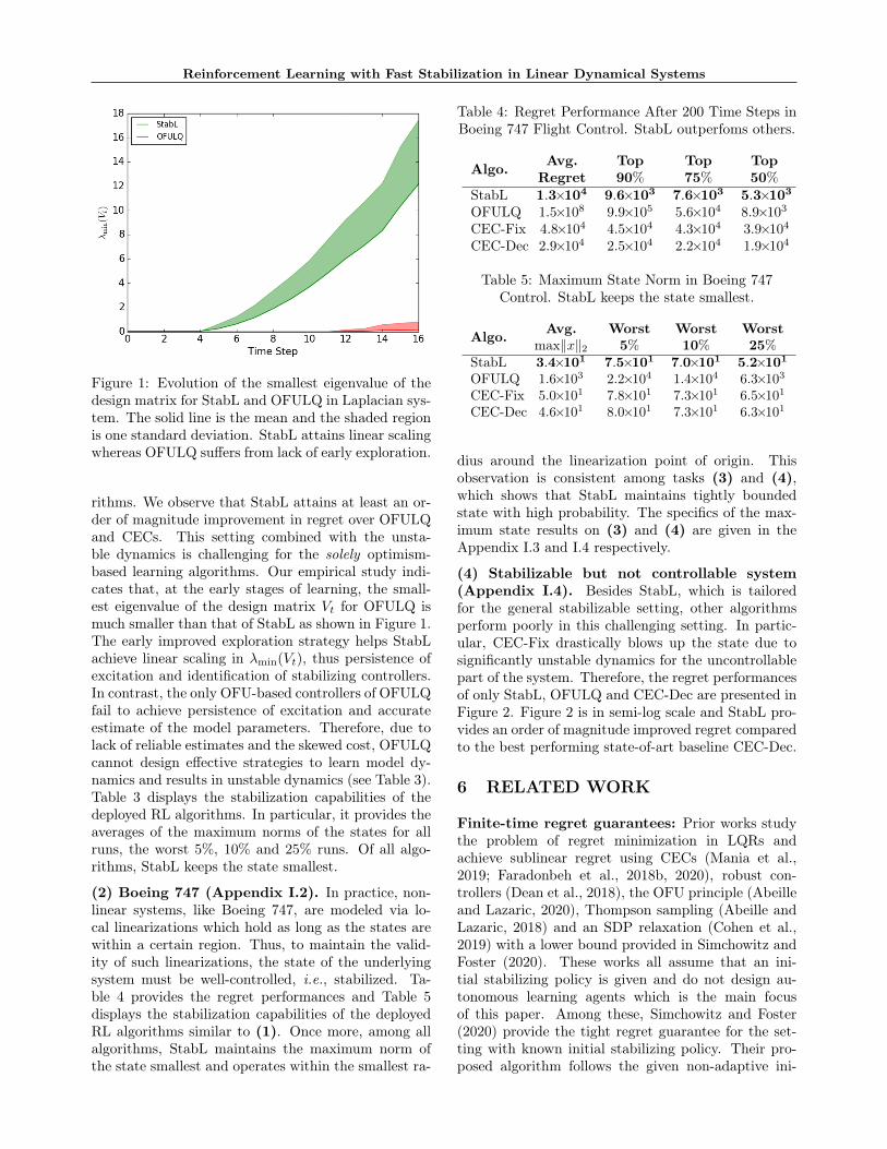
After showing the effect of fast stabilization, we canfinally present the regret upper bound of StabL.Theorem 4.2 (Regret of StabL). Suppose Assump-
Sahin Lale, Kamyar Azizzadenesheli, Babak Hassibi, Anima Anandkumar
Table 2: Regret Performance After 200 Time Steps inMarginally Unstable Laplacian System. StabL
outperfoms other algorithms by a significant margin
Algo. Avg.Regret
Top90%
Top75%
Top50%
StabL 1.5×10⁴ 1.3×10⁴ 1.1×10⁴ 8.9×10³
OFULQ 6.2×10¹⁰ 4.0×10⁶ 3.5×10⁵ 4.7×10⁴CEC-Fix 3.7×10¹⁰ 2.1×10⁴ 1.9×10⁴ 1.7×10⁴CEC-Dec 4.6×10⁴ 4.0×10⁴ 3.5×10⁴ 2.8×10⁴
tions 2.1 and 2.2 hold. For the given choices of Tw andTbase, with probability at least 1 − 4δ, StabL achievesregret of O
(poly(n, d)
√T log(1/δ)
), for long enough T .
The proofs and the exact expressions are presented inAppendix F. Here, we provide a proof sketch. The re-gret decomposition leverages the optimistic controllerdesign. Recall that for the early improved exploration,StabL applies independent perturbations through thecontroller yet still deploys the optimistic policy. Thus,we consider this external perturbation as a part of theunderlying system and study the regret obtained bythe improved exploration strategy separately.
In particular, denote the system evolution noise attime t as ζt. For t ≤ Tw, system evolution noise can beconsidered as ζt = B∗νt + wt and for t > Tw, ζt = wt.We denote the optimal average cost of system Θ underζt as J∗(Θ, ζt). Using the Bellman optimality equationfor LQR (Bertsekas, 1995), we consider the system evo-lution of the optimistic system Θt using the optimisticcontroller K(Θt) in parallel with the true system evo-lution of Θ∗ under K(Θt) such that they share thesame process noise (See details in Appendix F). Us-ing the confidence set construction, optimistic policy,Lemma 4.3, Assumption 2.2 and Lemma 2.1, we get aregret decomposition and bound each term separately.
At a high-level, the exact regret expression has a con-stant regret term due to early additional explorationfor Tw time-steps with exponential dimension depen-dency and a term that scales with square root ofthe duration of stabilizing adaptive control with poly-nomial dimension dependency, i.e. (n + d)n+dTw +poly(n, d)
√T − Tw. Note that Tw is a problem depen-
dent expression. Thus, for large enough T , the poly-nomial dependence dominates, giving Theorem 4.2.
5 EXPERIMENTS
In this section, we evaluate the performance of StabLin four adaptive control tasks: (1) a marginally unsta-ble Laplacian system (Dean et al., 2018), (2) the lon-gitudinal flight control of Boeing 747 with linearizeddynamics (Ishihara et al., 1992), (3) unmanned aerial
Table 3: Maximum State Norm in the LaplacianSystem. StabL keeps the state smallest
Algo. Avg.max∥x∥2
Worst5%
Worst10%
Worst25%
StabL 1.3×101 2.2×101 2.1×101 1.9×101
OFULQ 9.6×10³ 1.8×10⁵ 9.0×10⁴ 3.8×10⁴CEC-Fix 3.3×10³ 6.6×10⁴ 3.3×10⁴ 1.3×10⁴CEC-Dec 2.0×101 3.5×101 3.3×101 2.9× 101
vehicle (UAV) that operates in a 2-D plane (Zhaoet al., 2021), and (4) a stabilizable but not control-lable linear dynamical system. For each task, we com-pare StabL with three RL algorithms: (i) OFULQ ofAbbasi-Yadkori and Szepesvári (2011); (ii) certaintyequivalent controller with fixed isotropic perturbations(CEC-Fix), which is the standard baseline in controltheory; and (iii) certainty equivalent controller withdecaying isotropic perturbations (CEC-Dec), which isshown to achieve optimal regret with a given initialstabilizing policy (Simchowitz and Foster, 2020; Deanet al., 2018; Mania et al., 2019). In the implementa-tion of CEC-Fix and CEC-Dec, the optimal controlpolicies of the estimated model are deployed. Further-more, in finding the optimistic parameters for StabLand OFULQ, we use projected gradient descent withinthe confidence sets. We perform 200 independent runsfor each algorithm for 200 time steps starting fromx0 = 0. We present the performance of best parame-ter choices for each algorithm. For further details andthe experimental results please refer to Appendix I.
Before discussing the experimental results, we wouldlike to highlight the baselines choices. Unfortunately,there are only a few works in literature that considerRL in LQRs without a stabilizing controller. Theseworks are OFULQ of (Abbasi-Yadkori and Szepesvári,2011), (Abeille and Lazaric, 2018), and (Chen andHazan, 2020). Among these, (Chen and Hazan, 2020)considers LQRs with adversarial noise setting and de-ploys impractically large inputs, e.g. 1028 for task (1),whereas the algorithm of (Abeille and Lazaric, 2018)only works in scalar setting. These prohibit meaning-ful regret and stability comparisons, thus, we compareStabL against the only relevant comparison of OFULQamong these. Moreover, there are only a few and lim-ited experimental studies in the literature of RL inLQRs. Among these, (Dean et al., 2018; Faradonbehet al., 2018b, 2020) highlight the superior performanceof CEC-Dec. Therefore, we compare StabL againstCEC-Dec with the best-performing parameter choice,as well as the standard control baseline of CEC-Fix.
(1) Laplacian system (Appendix I.1). Table 2provides the regret performance for the average, top90%, top 75% and top 50% of the runs of the algo-
Reinforcement Learning with Fast Stabilization in Linear Dynamical Systems
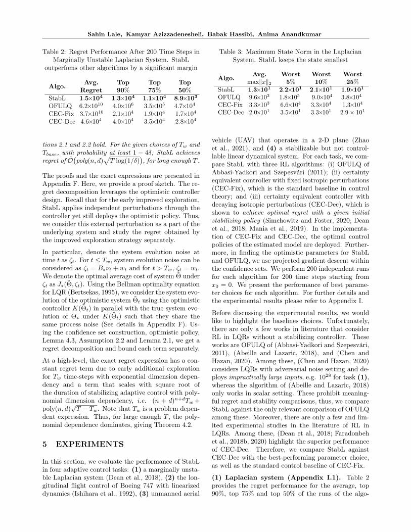
Figure 1: Evolution of the smallest eigenvalue of thedesign matrix for StabL and OFULQ in Laplacian sys-tem. The solid line is the mean and the shaded regionis one standard deviation. StabL attains linear scalingwhereas OFULQ suffers from lack of early exploration.
rithms. We observe that StabL attains at least an or-der of magnitude improvement in regret over OFULQand CECs. This setting combined with the unsta-ble dynamics is challenging for the solely optimism-based learning algorithms. Our empirical study indi-cates that, at the early stages of learning, the small-est eigenvalue of the design matrix Vt for OFULQ ismuch smaller than that of StabL as shown in Figure 1.The early improved exploration strategy helps StabLachieve linear scaling in λmin(Vt), thus persistence ofexcitation and identification of stabilizing controllers.In contrast, the only OFU-based controllers of OFULQfail to achieve persistence of excitation and accurateestimate of the model parameters. Therefore, due tolack of reliable estimates and the skewed cost, OFULQcannot design effective strategies to learn model dy-namics and results in unstable dynamics (see Table 3).Table 3 displays the stabilization capabilities of thedeployed RL algorithms. In particular, it provides theaverages of the maximum norms of the states for allruns, the worst 5%, 10% and 25% runs. Of all algo-rithms, StabL keeps the state smallest.
(2) Boeing 747 (Appendix I.2). In practice, non-linear systems, like Boeing 747, are modeled via lo-cal linearizations which hold as long as the states arewithin a certain region. Thus, to maintain the valid-ity of such linearizations, the state of the underlyingsystem must be well-controlled, i.e., stabilized. Ta-ble 4 provides the regret performances and Table 5displays the stabilization capabilities of the deployedRL algorithms similar to (1). Once more, among allalgorithms, StabL maintains the maximum norm ofthe state smallest and operates within the smallest ra-
Table 4: Regret Performance After 200 Time Steps inBoeing 747 Flight Control. StabL outperfoms others.
Algo. Avg.Regret
Top90%
Top75%
Top50%
StabL 1.3×10⁴ 9.6×10³ 7.6×10³ 5.3×10³
OFULQ 1.5×10⁸ 9.9×10⁵ 5.6×10⁴ 8.9×10³CEC-Fix 4.8×10⁴ 4.5×10⁴ 4.3×10⁴ 3.9×10⁴CEC-Dec 2.9×10⁴ 2.5×10⁴ 2.2×10⁴ 1.9×10⁴
Table 5: Maximum State Norm in Boeing 747Control. StabL keeps the state smallest.
Algo. Avg.max∥x∥2
Worst5%
Worst10%
Worst25%
StabL 3.4×101 7.5×101 7.0×101 5.2×101
OFULQ 1.6×10³ 2.2×10⁴ 1.4×10⁴ 6.3×10³CEC-Fix 5.0×101 7.8×101 7.3×101 6.5×101CEC-Dec 4.6×101 8.0×101 7.3×101 6.3×101
dius around the linearization point of origin. Thisobservation is consistent among tasks (3) and (4),which shows that StabL maintains tightly boundedstate with high probability. The specifics of the max-imum state results on (3) and (4) are given in theAppendix I.3 and I.4 respectively.
(4) Stabilizable but not controllable system(Appendix I.4). Besides StabL, which is tailoredfor the general stabilizable setting, other algorithmsperform poorly in this challenging setting. In partic-ular, CEC-Fix drastically blows up the state due tosignificantly unstable dynamics for the uncontrollablepart of the system. Therefore, the regret performancesof only StabL, OFULQ and CEC-Dec are presented inFigure 2. Figure 2 is in semi-log scale and StabL pro-vides an order of magnitude improved regret comparedto the best performing state-of-art baseline CEC-Dec.
6 RELATED WORK
Finite-time regret guarantees: Prior works studythe problem of regret minimization in LQRs andachieve sublinear regret using CECs (Mania et al.,2019; Faradonbeh et al., 2018b, 2020), robust con-trollers (Dean et al., 2018), the OFU principle (Abeilleand Lazaric, 2020), Thompson sampling (Abeille andLazaric, 2018) and an SDP relaxation (Cohen et al.,2019) with a lower bound provided in Simchowitz andFoster (2020). These works all assume that an ini-tial stabilizing policy is given and do not design au-tonomous learning agents which is the main focusof this paper. Among these, Simchowitz and Foster(2020) provide the tight regret guarantee for the set-ting with known initial stabilizing policy. Their pro-posed algorithm follows the given non-adaptive ini-

Sahin Lale, Kamyar Azizzadenesheli, Babak Hassibi, Anima Anandkumar
Figure 2: Regret Comparison of three algorithms incontrolling a stabilizable but not controllable system.The solid lines are the average regrets and the shadedregions are the quarter standard deviations.
tial stabilizing policy for a long period of time withisotropic perturbations. Thus, they provide an order-optimal theoretical regret upper bound with an addi-tional large constant regret. However, in many ap-plications, e.g. medical, such constant regret, andnon-adaptive controllers are not tolerable. StabL aimsto address these challenges and provide an adaptivealgorithm that can be deployed in practice. More-over, StabL achieves significantly improved perfor-mance over the prior baseline RL algorithms in variousadaptive control tasks (Section 5).
Finding a stabilizing controller: Similar to the re-gret minimization, there has been a growing interestin finite-time stabilization of linear dynamical systems(Dean et al., 2019; Faradonbeh et al., 2018a, 2019).Among these works, Faradonbeh et al. (2018a) is theclosest to our work. However, there are significant dif-ferences in the methods and the span of the results. InFaradonbeh et al. (2018a), random linear controllersare used solely for finding a stabilizing set without acontrol goal. This results in the explosion of state, pre-sumably exponentially in time, leading to a regret thatscales exponentially in time. The proposed methodprovides many insightful aspects for finding a stabiliz-ing set in finite-time, yet a cost analysis of this processor an adaptive control policy are not provided. More-over, the stabilizing set in Faradonbeh et al. (2018a)relates to the minimum value that satisfies a specificcondition for the roots of a polynomial. This results ina somewhat implicit sample complexity for construct-ing such a set. On the other hand, in this work, weprovide a complete study of an autonomous learningalgorithm for the online LQR problem. Among our re-sults, we give an explicit formulation of the stabilizing
set and a sample complexity that only relates to theminimal stabilizability information of the system.
Generalized LQR setting: Another line of researchconsiders the generalizations of the online LQR prob-lem under partial observability (Lale et al., 2020a,b,c;Mania et al., 2019; Simchowitz et al., 2020) or ad-versarial disturbances (Hazan et al., 2019; Chen andHazan, 2020). These works either assume a given sta-bilizing controller or open-loop stable system dynam-ics, except Chen and Hazan (2020). Independentlyand concurrently, the recent work by Chen and Hazan(2020) designs an autonomous learning algorithm andregret guarantees that are similar to the current work.However, the approaches and the settings have ma-jor differences. Chen and Hazan (2020) considers therestrictive setting of controllable systems, yet withadversarial disturbances and general cost functions.They inject significantly big inputs, exponential insystem parameters, with a pure exploration intent toguarantee the recovery of system parameters and sta-bilization. This negatively affects the practicality ofthe algorithm. On the other hand, in this work, we in-ject isotropic Gaussian perturbations to improve theexploration in the stochastic (sub-Gaussian processnoise) stabilizable LQR while still aiming to control,i.e. no pure exploration phase. This yields a practi-cal RL algorithm StabL that attains state-of-the-artperformance.
7 CONCLUSION
In this paper, we propose an RL framework, StabL,that follows OFU principle to balance between explo-ration and exploitation in interaction with LQRs. Weshow that if an additional random exploration is en-forced in the early stages of the agent’s interactionwith the environment, StabL has the guarantee to de-sign a stabilizing controller sooner. We then show thatwhile the agent enjoys the benefit of stable dynamicsin further stages, the additional exploration does notalter the early performance of the agent considerably.Finally, we prove that the regret upper bound of StabLis O(
√T ) with polynomial dependence in the problem
dimensions of the LQRs in stabilizable systems.
Our results highlight the benefit of early improved ex-ploration to achieve improved regret at the expense ofa slight increase in regret in the early stages. An im-portant future direction is to study this phenomenon inmore challenging online control problems in linear sys-tems, e.g., under partially observability. Another in-teresting direction is to combine this mindset with theexisting state-of-the-art model-based RL approachesfor the general systems and study their performance.

Reinforcement Learning with Fast Stabilization in Linear Dynamical Systems
References
Dimitri P Bertsekas. Dynamic programming and op-timal control, volume 2. Athena scientific Belmont,MA, 1995.
Yasin Abbasi-Yadkori and Csaba Szepesvári. Regretbounds for the adaptive control of linear quadraticsystems. In Proceedings of the 24th Annual Confer-ence on Learning Theory, pages 1–26, 2011.
Marc Abeille and Alessandro Lazaric. Improved regretbounds for thompson sampling in linear quadraticcontrol problems. In International Conference onMachine Learning, pages 1–9, 2018.
Xinyi Chen and Elad Hazan. Black-box controlfor linear dynamical systems. arXiv preprintarXiv:2007.06650, 2020.
Mohamad Kazem Shirani Faradonbeh, Ambuj Tewari,and George Michailidis. Finite time adap-tive stabilization of lq systems. arXiv preprintarXiv:1807.09120, 2018a.
Marc Abeille and Alessandro Lazaric. Efficientoptimistic exploration in linear-quadratic regula-tors via lagrangian relaxation. arXiv preprintarXiv:2007.06482, 2020.
Max Simchowitz and Dylan J Foster. Naive explo-ration is optimal for online lqr. arXiv preprintarXiv:2001.09576, 2020.
Marc Abeille and Alessandro Lazaric. Thompson sam-pling for linear-quadratic control problems. arXivpreprint arXiv:1703.08972, 2017.
Sarah Dean, Horia Mania, Nikolai Matni, BenjaminRecht, and Stephen Tu. Regret bounds for robustadaptive control of the linear quadratic regulator.In Advances in Neural Information Processing Sys-tems, pages 4188–4197, 2018.
Horia Mania, Stephen Tu, and Benjamin Recht. Cer-tainty equivalent control of lqr is efficient. arXivpreprint arXiv:1902.07826, 2019.
Tze Leung Lai and Herbert Robbins. Asymptoticallyefficient adaptive allocation rules. Advances in ap-plied mathematics, 6(1):4–22, 1985.
Sergio Bittanti, Marco C Campi, et al. Adaptive con-trol of linear time invariant systems: the “bet on thebest” principle. Communications in Information &Systems, 6(4):299–320, 2006.
Thomas Kailath, Ali H Sayed, and Babak Hassibi. Lin-ear estimation, 2000.
Bernard Friedland. Control system design: an intro-duction to state-space methods. Courier Corpora-tion, 2012.
Alon Cohen, Tomer Koren, and Yishay Mansour.Learning linear-quadratic regulators efficiently with
only√T regret. arXiv preprint arXiv:1902.06223,
2019.
Elad Hazan, Sham M Kakade, and Karan Singh.The nonstochastic control problem. arXiv preprintarXiv:1911.12178, 2019.
Tadashi Ishihara, Hai-Jiao Guo, and Hiroshi Takeda.A design of discrete-time integral controllers withcomputation delays via loop transfer recovery. Au-tomatica, 28(3):599–603, 1992.
Feiran Zhao, Keyou You, and Tamer Basar. Infinite-horizon risk-constrained linear quadratic regulatorwith average cost. arXiv preprint arXiv:2103.15363,2021.
Mohamad Kazem Shirani Faradonbeh, Ambuj Tewari,and George Michailidis. Input perturbations foradaptive regulation and learning. arXiv preprintarXiv:1811.04258, 2018b.
Mohamad Kazem Shirani Faradonbeh, Ambuj Tewari,and George Michailidis. On adaptive linear–quadratic regulators. Automatica, 117:108982, 2020.
Sarah Dean, Horia Mania, Nikolai Matni, BenjaminRecht, and Stephen Tu. On the sample complexityof the linear quadratic regulator. Foundations ofComputational Mathematics, pages 1–47, 2019.
Mohamad Kazem Shirani Faradonbeh, Ambuj Tewari,and George Michailidis. Randomized algorithmsfor data-driven stabilization of stochastic linear sys-tems. In 2019 IEEE Data Science Workshop (DSW),pages 170–174. IEEE, 2019.
Sahin Lale, Kamyar Azizzadenesheli, Babak Hassibi,and Anima Anandkumar. Regret minimization inpartially observable linear quadratic control. arXivpreprint arXiv:2002.00082, 2020a.
Sahin Lale, Kamyar Azizzadenesheli, Babak Hassibi,and Anima Anandkumar. Regret bound of adaptivecontrol in linear quadratic gaussian (lqg) systems.arXiv preprint arXiv:2003.05999, 2020b.
Sahin Lale, Kamyar Azizzadenesheli, Babak Hassibi,and Anima Anandkumar. Logarithmic regret boundin partially observable linear dynamical systems.arXiv preprint arXiv:2003.11227, 2020c.
Max Simchowitz, Karan Singh, and Elad Hazan. Im-proper learning for non-stochastic control. arXivpreprint arXiv:2001.09254, 2020.
Alon Cohen, Avinatan Hassidim, Tomer Koren,Nevena Lazic, Yishay Mansour, and Kunal Tal-war. Online linear quadratic control. arXiv preprintarXiv:1806.07104, 2018.
Asaf Cassel, Alon Cohen, and Tomer Koren. Logarith-mic regret for learning linear quadratic regulatorsefficiently. arXiv preprint arXiv:2002.08095, 2020.

Sahin Lale, Kamyar Azizzadenesheli, Babak Hassibi, Anima Anandkumar
Yasin Abbasi-Yadkori, Dávid Pál, and CsabaSzepesvári. Improved algorithms for linear stochas-tic bandits. In Advances in Neural Information Pro-cessing Systems, pages 2312–2320, 2011.
Tze Leung Lai, Ching Zong Wei, et al. Least squaresestimates in stochastic regression models with ap-plications to identification and control of dynamicsystems. The Annals of Statistics, 10(1):154–166,1982.
Arthur Becker, P Kumar, and Ching-Zong Wei. Adap-tive control with the stochastic approximation algo-rithm: Geometry and convergence. IEEE Transac-tions on Automatic Control, 30(4):330–338, 1985.
PR Kumar. Convergence of adaptive control schemesusing least-squares parameter estimates. IEEETransactions on Automatic Control, 35(4):416–424,1990.
Yasin Abbasi-Yadkori, Nevena Lazic, and CsabaSzepesvári. Regret bounds for model-free linearquadratic control. arXiv preprint arXiv:1804.06021,2018.
Stephen Tu and Benjamin Recht. Least-squares tem-poral difference learning for the linear quadratic reg-ulator. In International Conference on MachineLearning, pages 5005–5014. PMLR, 2018.

Supplementary Material:Reinforcement Learning with Fast Stabilization
in Linear Dynamical Systems
In Appendix A, we first provide a discussion on how stabilizability and (κ, γ)-stabilizable systems are equivalent.Then we prove that for (κ, γ)-stabilizable systems the unique positive definite solution to the DARE given in (2) isbounded. Finally, we show that there exists a stabilizing neighborhood (ball) around the true model parametersin which the optimal controllers of the models within this ball stabilize the underlying system in Appendix A.In Appendix B, we show that due to improved exploration strategy, the regularized design matrix Vt has itsminimum eigenvalue scaling linearly over time, which guarantees the persistently exciting inputs for finding thestabilizing neighborhood and stabilizing controllers after the adaptive control with improved exploration phase.The exact definition of σ⋆ is also given in Lemma B.3 in Appendix B. We provide the system identificationand confidence set constructions with their guarantees (both in terms of self-normalized and spectral norm)in Appendix C. In Appendix D, we provide the boundedness guarantees for the system’s state throughout theexecution of StabL and provide the proof of Lemma 4.3. The precise definition of Tw, which was omitted inthe main text, is also given in (31) in Appendix D. We provide the regret decomposition in Appendix E andwe analyze each term in this decomposition and give the proof of the main result of the paper in Appendix F.In Appendix G, we compare the results with Abbasi-Yadkori and Szepesvári (2011) and show it subsumes andimproves the prior work. Appendix H provides the technical theorems and lemmas that are utilized in the proofs.Finally, in Appendix I, we provide the details on the experiments including the dynamics of the adaptive controltasks, parameter choices for the algorithms and additional experimental results.
A STABILIZABILITY OF THE UNDERLYING SYSTEM
In this section, we first show that (κ, γ)-stabilizability is merely a quantification of stabilizability. Then, we showthat the given systems (both controllable and stabilizable) DARE has a unique positive definite solution. Finally,we show that combining two prior results, there exists a stabilizing neighborhood round the system parametersthat any controller designed using parameters in that neighborhood stabilizes the system.
A.1 (κ, γ)-stabilizability
Any stabilizable system is also (κ, γ)-stabilizable for some κ and γ and the conversely (κ, γ)-stabilizability impliesstabilizability. In particular, for all stabilizable systems, by setting 1 − γ = ρ(A∗ + B∗K(Θ∗)) and κ to be thecondition number of P (Θ∗)
1/2 where P (Θ∗) is the positive definite matrix that satisfies the following Lyapunovequation:
(A∗ +B∗K(Θ∗))⊤P (Θ∗)(A∗ +B∗K(Θ∗)) ⪯ P (Θ∗), (3)
one can show that A∗ + B∗K(Θ∗) = HLH−1, where H = P (Θ∗)−1/2 and L = P (Θ∗)
1/2(A∗ +B∗K(Θ∗))P (Θ∗)
−1/2 with ∥H∥∥H−1∥ ≤ κ, and ∥L∥ ≤ 1− γ (Lemma B.1 of Cohen et al. (2018)).
Sahin Lale, Kamyar Azizzadenesheli, Babak Hassibi, Anima Anandkumar
A.2 Bound on the Solution of DARE for (κ, γ)-Stabilizable Systems, Proof of Lemma 2.1
Proof of Lemma 2.1: Recall the DARE given in (2). The solution of this equation corresponds to recursivelyapplying the following
∥P∗∥ = ∥∑∞
t=0
((A∗ +B∗K(Θ∗))
t)⊤ (
Q+K(Θ∗)⊤RK(Θ∗)
)(A∗ +B∗K(Θ∗))
t ∥
= ∥∑∞
t=0
(HLtH−1
)⊤ (Q+K(Θ∗)
⊤RK(Θ∗)) (
HLtH−1)∥
≤ α(1 + ∥K(Θ∗)∥2)∥H∥2∥H−1∥2∑∞
t=0∥L∥2t (4)
≤ αγ−1κ2(1 + κ2) (5)
where (4) follows from the upper bound on ∥Q∥, ∥R∥ ≤ α and (5) follows from the definition of (κ, γ)-stabilizability.
A.3 Stabilizing Neighborhood Around the System Parameters
Theorem A.1 (Unique Positive Definite Solution to DARE, (Bertsekas, 1995)). For Θ∗ = (A∗, B∗), If (A∗, B∗)is stabilizable and (C,A∗) is observable for Q = C⊤C, or Q is positive definite, then there exists a unique,bounded solution, P (Θ∗), to the DARE:
P (Θ∗) = A⊤∗ P (Θ∗)A∗ +Q−A⊤
∗ P (Θ∗)B∗(R+B⊤
∗ P (Θ∗)B∗)−1
B⊤∗ P (Θ∗)A∗. (6)
The controller K(Θ∗) = −(R+B⊤
∗ P (Θ∗)B∗)−1
B⊤∗ P (Θ∗)A∗ produces stable closed-loop system, ρ(A∗ +
B∗K(Θ∗)) < 1.
This result shows that, for we get unique positive definite solution to DARE for stabilizable systems. Let J∗ ≤ J .The following lemma is introduced in Simchowitz and Foster (2020) and shows that if the estimation error on thesystem parameters is small enough, then the performance of the optimal controller synthesized by these modelparameter estimates scales quadratically with the estimation error.
Lemma A.1 ((Simchowitz and Foster, 2020)). For constants C0 = 142∥P∗∥8 and ϵ = 54∥P∗∥5 , such that, for any
0 ≤ ε ≤ ϵ and for ∥Θ′−Θ∗∥ ≤ ε, the infinite horizon performance of the policy K(Θ′) on Θ∗ obeys the following,
J(K(Θ′), A∗, B∗, Q,R)− J∗ ≤ C0ε2.
This result shows that there exists a ϵ-neighborhood around the system parameters that stabilizes the system.This result further extended to quantify the stability in Cassel et al. (2020).
Lemma A.2 (Lemma 41 in Cassel et al. (2020)). Suppose J(K(Θ′), A∗, B∗, Q,R) ≤ J ′ for the LQR underAssumption 2.1, then K(Θ′) produces (κ′, γ′)-stable closed-loop dynamics where κ′ =
√J ′
ασ2w
and γ′ = 1/2κ′2.
Combining these results, we obtain the proof of Lemma 4.2.
Proof of Lemma 4.2: Under Assumptions 2.1 & 2.2, for ε ≤ min√J /C0, ϵ, we obtain
J(K(Θ′), A∗, B∗, Q,R) ≤ 2J . Plugging this into Lemma A.2 gives the presented result.
B SMALLEST SINGULAR VALUE OF REGULARIZED DESIGN MATRIX Vt
In this section, we show that improved exploration of StabL provides persistently exciting inputs, which will beused to enable reaching a stabilizing neighborhood around the system parameters. In other words, we will lowerbound the smallest eigenvalue of the regularized design matrix, Vt. The analysis generalizes the lower bound onsmallest eigenvalue of the sample covariance matrix in Theorem 20 of (Cohen et al., 2019) for the general caseof subgaussian noise.

Reinforcement Learning with Fast Stabilization in Linear Dynamical Systems
For the state xt, and input ut, we have:
xt = A∗xt−1 +B∗ut−1 + wt−1, and ut = K(Θt−1)xt + νt (7)
Let ξt = zt − E [zt|Ft−1]. Using the equalities in (7), and the fact that wt and νt are Ft measurable, we writeE[ξtξ
⊤t |Ft−1
]as follows.
E[ξtξ
⊤t |Ft−1
]=
(I
K(Θt−1)
)E[wtw
⊤t |Ft−1
]( I
K(Θt−1)
)⊤
+
(0 00 E
[νtν
⊤t |Ft−1
] )=
(I
K(Θt−1)
)(σ2
wI)
(I
K(Θt−1)
)⊤
+
(0 00 σ2
νI
)(8)
=
(σ2wI σ2
wK(Θt−1)⊤
σ2wK(Θt−1) σ2
wK(Θt−1)K(Θt−1)⊤ + 2κ2σ2
wI
)(9)
⪰ σ2w
(I K(Θt−1)
⊤
K(Θt−1) 2K(Θt−1)K(Θt−1)⊤ + I/2
)(10)
=σ2w
2I + σ2
w
(1√2I√
2K(Θt−1)
)(1√2I√
2K(Θt−1)
)⊤
(11)
⪰ σ2w
2I (12)
where (9) follows from σ2ν = 2κ2σ2
w and (10) follows from the fact that κ ≥ 1 and ∥K(Θt−1)∥ ≤ κ for all t. Letst = v⊤ξt for any unit vector v ∈ Rn+d. (12) shows that that Var [st|Ft−1] ≥ σ2
w
2 .
Lemma B.1. Suppose the system is stabilizable and we are in adaptive control with improved exploration phaseof StabL. Denote st = v⊤ξt where v ∈ Rn+d is any unit vector. Let σν := ((1+κ)2+2κ2)σ2
w. For a given positiveσ21, let Et be an indicator random variable that equals 1 if s2t > σ2
1 and 0 otherwise. Then for any positive σ21,
and σ22, such that σ2
1 ≤ σ22, we have
E [Et|Ft−1] ≥σ2w
2 − σ21 − 4σ2
ν(1 +σ22
2σ2ν) exp(
−σ22
2σ2ν)
σ22
(13)
Note that, for any σν ≥ σw, there is a pair (σ21 , σ
22) such that the right hand side of (13) is positive.
Proof. Using the lower bound on the variance of st, we have,
σ2w
2≤ E
[s2t1(s
2t < σ2
1)|Ft−1
]+ E
[s2t1(s
2t ≥ σ2
1)|Ft−1
]≤ σ2
1 + E[s2t1(s
2t ≥ σ2
1)|Ft−1
]Now, deploying the fact that both νt and wt, for any t, are sub-Gaussian given Ft−1, have that ξt is also sub-Gaussian vector. Therefore, st is a sub-Gaussian random variable with parameter σν , where σν := ((1 + κ)2 +2κ2)σ2
w.
σ2w
2− σ2
1 ≤ E[s2t1(s
2t ≥ σ2
1)|Ft−1
]= E
[s2t1(σ
22 ≥ s2t ≥ σ2
1)|Ft−1
]+ E
[s2t1(s
2t ≥ σ2
2)|Ft−1
](14)
For the second term in the right hand side of the (14), under the considerations of Fubini’s and Radon–Nikodym

Sahin Lale, Kamyar Azizzadenesheli, Babak Hassibi, Anima Anandkumar
theorems, we derive the following equality,∫s2≥σ2
2
P(s2t ≥ s2|Ft−1)ds2 =
∫s2≥σ2
2
∫s′2≥s2
−dP(s2t ≥ s′2|Ft−1)
ds′2ds′2ds2
=
∫s′2≥σ2
2
∫s′2≥s2≥σ2
2
−dP(s2t ≥ s′2|Ft−1)
ds′2ds′2ds2
=
∫s′2≥σ2
2
∫s′2≥s2≥σ2
2
−dP(s2t ≥ s′2|Ft−1)
ds′2ds2ds′2
=
∫s′2≥σ2
2
−dP(s2t ≥ s′2|Ft−1)
ds′2(s′2 − σ2
2)ds′2
= E[s2t1(s
2t ≥ σ2
2)|Ft−1
]− σ2
2
∫s′2≥σ2
2
−dP(s2t ≥ s′2|Ft−1)
ds′2ds′2
= E[s2t1(s
2t ≥ σ2
2)|Ft−1
]− σ2
2 P(s2t ≥ σ22 |Ft−1),
resulting in the following equality,
E[s2t1(s
2t ≥ σ2
2)|Ft−1
]=
∫s2≥σ2
2
P(s2t ≥ s2|Ft−1)ds2 + σ2
2 P(s2t ≥ σ22 |Ft−1). (15)
Using this equality, we extend the (14) as follows,
σ2w
2− σ2
1 ≤ E[s2t1(σ
22 ≥ s2t ≥ σ2
1)|Ft−1
]+
∫s2≥σ2
2
P(s2t ≥ s2|Ft−1)ds2 + σ2
2 P(s2t ≥ σ22 |Ft−1)
≤ σ22 E
[1(σ2
2 ≥ s2t ≥ σ21)|Ft−1
]+
∫s2≥σ2
2
P(s2t ≥ s2|Ft−1)ds2 + σ2
2 P(s2t ≥ σ22 |Ft−1)
≤ σ22 E [Et|Ft−1] +
∫s2≥σ2
2
P(s2t ≥ s2|Ft−1)ds2 + σ2
2 P(s2t ≥ σ22 |Ft−1). (16)
Rearranging this inequality, we have,
E [Et|Ft−1] ≥σ2w
2 − σ21 −
∫s2≥σ2
2P(s2t ≥ s2|Ft−1)ds
2 − σ22 P(s2t ≥ σ2
2 |Ft−1)
σ22
≥σ2w
2 − σ21 − 2
∫s2≥σ2
2exp(−s2
2σ2ν)ds2 − 2σ2
2 exp(−σ2
2
2σ2ν)
σ22
≥σ2w
2 − σ21 − 4σ2
ν exp(−σ2
2
2σ2ν)− 2σ2
2 exp(−σ2
2
2σ2ν)
σ22
=
σ2w
2 − σ21 − 4σ2
ν(1 +σ22
2σ2ν) exp(
−σ22
2σ2ν)
σ22
(17)
The inequality in (17) holds for any σ21 ≤ σ2
2 , therefore, the stated lower-bound on E [Et|Ft−1] in the mainstatement holds.
For the choices of σ21 and σ2
2 that makes right hand side of (13) positive, let cp denote the right hand side of
(13), cp =
σ2w2 −σ2
1−4σ2ν(1+
σ22
2σ2ν) exp(
−σ22
2σ2ν)
σ22
.
Lemma B.2. Consider st = v⊤zt where v ∈ Rn+d is any unit vector. Let Et be an indicator random variablethat equal 1 if s2t > σ2
1/4 and 0 otherwise. Then, there exist a positive pair σ21, and σ2
2, and a constant cp > 0,such that E
[Et|Ft−1
]≥ c′p > 0.

Reinforcement Learning with Fast Stabilization in Linear Dynamical Systems
Proof. Using the Lemma B.1, we know that for st = v⊤ξt, we have |st| ≥ σ1 with a non-zero probability cp. Onthe other hand, we have that,
st = v⊤zt = v⊤ξt + v⊤E [zt|Ft−1] = st + v⊤E [zt|Ft−1]
Therefore, we have, |st| =∣∣st + v⊤E [zt|Ft−1]
∣∣. Using this equality, if∣∣v⊤E [zt|Ft−1]
∣∣ ≤ σ1/2, since |st| ≥ σ1
with probability cp, we have |st| ≥ σ1/2 with probability cp.
In the following, we consider the case where∣∣v⊤E [zt|Ft−1]
∣∣ ≥ σ1/2. For a constant σ3, using a similar derivationas in (15) and (16), we have
E[s2t |Ft−1
]= E
[s2t1(σ3 < st < 0)|Ft−1
]+ E
[s2t1(σ3 > st > 0)|Ft−1
]+ E
[s2t1(s
2t ≥ σ2
3)|Ft−1
]= E
[s2t1(σ3 < st < 0)|Ft−1
]+ E
[s2t1(σ3 > st > 0)|Ft−1
]+ 4σ2
ν(1 +σ22
2σ2ν
) exp(−σ2
2
2σ2ν
)
Using the lower bound in the variance results in,
σ2w
2≤ E
[s2t1(σ3 < st < 0)|Ft−1
]+ E
[s2t1(σ3 > st > 0)|Ft−1
]+ 4σ2
ν(1 +σ23
2σ2ν
) exp(−σ2
3
2σ2ν
)
Therefore,
σ2w
2− 4σ2
ν(1 +σ23
2σ2ν
) exp(−σ2
3
2σ2ν
) ≤ E[s2t1(σ3 < st < 0)|Ft−1
]+ E
[s2t1(σ3 > st > 0)|Ft−1
]= σ2
3
(E[s2tσ23
1(−σ3 < st < 0)|Ft−1
]+ E
[s2tσ23
1(σ3 > st > 0)|Ft−1
])≤ σ2
3
(E[|st|σ3
1(−σ3 < st < 0)|Ft−1
]+ E
[stσ31(σ3 > st > 0)|Ft−1
])(18)
Note the for a large enough σ3, the second term on the left hand side vanishes. Since we have E [st|Ft−1] = 0,we write the following, to further analyze the right hand side of (18),
E [st|Ft−1] = E [st1(st < 0)|Ft−1] + E [st1(st > 0)|Ft−1] = 0
→ E [|st|1(st < 0)|Ft−1] = E [st1(st > 0)|Ft−1]
Note that, since st is sub-Gaussian variable, and has bounded away from zero variance, we haveE [1(st < 0)|Ft−1] + E [1(st > 0)|Ft−1] is bounded away from zero. We write this equality as follows:
E [|st|1(−σ3 < st < 0)|Ft−1] + E [|st|1(st ≤ −σ3)|Ft−1]
= E [st1(σ3 > st > 0)|Ft−1] + E [st1(st ≥ σ3)|Ft−1]
With rearranging this equality, and upper bounding the first term on the left hand side, we have
E [|st|1(−σ3 < st < 0)|Ft−1] ≤ E [st1(σ3 > st > 0)|Ft−1] + E [st1(st ≥ σ3)|Ft−1]
≤ E [st1(σ3 > st > 0)|Ft−1] + σ2ν exp(
−σ23
2σ2ν
) (19)
similarly we have
E [st1(σ3 > st > 0)|Ft−1] ≤ E [|st|1(−σ3 < st < 0)|Ft−1] + σ2ν exp(
−σ23
2σ2ν
) (20)
Using the inequality (19) on the right hand side of (18), we have

Sahin Lale, Kamyar Azizzadenesheli, Babak Hassibi, Anima Anandkumar
σ2w
2 − 4σ2ν(1 +
σ23
2σ2ν) exp(
−σ23
2σ2ν)
σ23
≤ E[|st|σ3
1(−σ3 < st < 0)|Ft−1
]+ E
[stσ31(σ3 > st > 0)|Ft−1
]≤ 2E
[stσ31(σ3 > st > 0)|Ft−1
]+ σ2
ν exp(−σ2
3
2σ2ν
)
≤ 2E [1(σ3 > st > 0)|Ft−1] + σ2ν exp(
−σ23
2σ2ν
)
≤ 2E [1(st > 0)|Ft−1] + σ2ν exp(
−σ23
2σ2ν
)
Similarly, using (19) on the right hand side of (18) we have
σ2w
2 − 4σ2ν(1 +
σ23
2σ2ν) exp(
−σ23
2σ2ν)
σ23
≤ E[|st|σ3
1(−σ3 < st < 0)|Ft−1
]+ E
[stσ31(σ3 > st > 0)|Ft−1
]≤ 2E [1(st < 0)|Ft−1] + σ2
ν exp(−σ2
3
2σ2ν
)
Therefore, it results in the two following lower bounds,
E [1(st < 0)|Ft−1] ≥σ2w
2 − 4σ2ν(1 +
σ23
2σ2ν) exp(
−σ23
2σ2ν)
2σ23
− 0.5σ2ν exp(
−σ23
2σ2ν
)
E [1(st > 0)|Ft−1] ≥σ2w
2 − 4σ2ν(1 +
σ23
2σ2ν) exp(
−σ23
2σ2ν)
2σ23
− 0.5σ2ν exp(
−σ23
2σ2ν
) (21)
Choosing σ3 sufficiently large results in the right hand sides in inequalities (21) to be positive and boundedaway form zero. Let c′′p > 0 denote the right hand sides in the (21). We use this fact to analyze st when∣∣v⊤E [zt|Ft−1]
∣∣ ≥ σ1/2.
When v⊤E [zt|Ft−1] ≥ σ1/2, since probability c′′p , st is positive, therefore, |st| ≥ σ1/2 with probability c′′p . Whenv⊤E [zt|Ft−1] ≤ −σ1/2, since probability c′′p , st is negative, therefore, |st| ≥ σ1/2 with probability c′′p .
Therefore, overall, with probability c′p := mincp, c′′p, we have that |st| ≥ σ1/2, resulting in the statement of thelemma.
Lemma B.3 (Precise version of Lemma 4.1, Persistence of Excitation During the Extra Exploration). If theduration of the adaptive control with improved exploration Tw ≥ 6n
c′plog(12/δ), then with probability at least 1− δ,
StabL hasλmin(VTw
) ≥ σ2⋆Tw,
for σ2⋆ =
c′pσ21
16 .
Proof. Let Ut = Et−Et
[Et|Ft−1
]. Then Ut is a martingale difference sequence with |Ut| ≤ 1. Applying Azuma’s
inequality, we have that with probability at least 1− δ
Tw∑t=1
Ut ≥ −√2Tw log
1
δ
Using the Lemma B.2, we have
Tw∑t
Et ≥Tw∑t
Et
[Et|Ft−n
]−√2Tw log
1
δ
≥ c′pTw −√2Tw log
1
δ

Reinforcement Learning with Fast Stabilization in Linear Dynamical Systems
where for Tw ≥ 8 log(1/δ)/c′2p , we have∑Tw
t Et ≥c′p2 Tw. Now, for any unit vector v, define st = v⊤zt, therefore
from the definition of Et we have,
v⊤VTwv =
Tw∑t
s2t ≥ Etσ21/4 ≥
c′pσ21
8Tw
This inequality hold for a given v. In the following we show a similar inequality for all v together. Similar to theTheorem 20 in (Cohen et al., 2019), consider a 1/4-net of Sn+d−1, N (1/4) and set MTw
:= V −1/2Tw
v/∥V −1/2Tw
v∥ :
v ∈ N (1/4). These two sets have at most 12n+d−1 members. Using union bound over members of this set,
when Tw ≥ 20c′2p
((n + d) + log(1/δ)), we have that v⊤VTwv ≥ c′pσ
21
8 Tw for all v ∈ MTwwith a probability at least
1− δ. Using the definition of members in MTw, for each v ∈ N (1/4), we have v⊤V −1
Twv ≤ 8
Twc′pσ21. Let vn denote
the eigenvector of the largest eigenvalue of V −1Tw
, and a vector v′ ∈ N (1/4) such that ∥vn − v′∥ ≤ 1/4. Then wehave
∥V −1Tw
∥ = v⊤n V−1Tw
vn = v′⊤V −1Tw
v′ + (vn − v′)⊤V −1Tw
(zn + v′)
≤ 8
Twc′pσ21
+ ∥vn − v′∥∥V −1Tw
∥∥zn + v′∥ ≤ 8
Twc′pσ21
+ ∥V −1Tw
∥/2
Rearranging, we get that ∥V −1Tw
∥ ≤ 16Twc′pσ
21. Therefore, the advertised bound holds for Tw ≥ 20
c′2p((n+d)+log(1/δ))
with probability at least 1− δ.
C SYSTEM IDENTIFICATION & CONFIDENCE SET CONSTRUCTION
To have completeness, for the proof of Lemma 4.1 we first provide the proof for confidence set construction bor-rowed from Abbasi-Yadkori and Szepesvári (2011), since Lemma 4.1 builds upon this confidence set construction.First let
κe =
(σw
σ⋆
√n(n+ d) log
(1 +
cT (1 + κ2)(n+ d)2(n+d)
λ(n+ d)
)+ 2n log
1
δ+
√λS
)(22)
Proof. Define Θ⊤∗ = [A,B] and zt =
[x⊤t u
⊤t
]⊤. The system in (1) can be characterized equivalently as
xt+1 = Θ⊤∗ zt + wt
Given a single input-output trajectory xt, utTt=1, one can rewrite the input-output relationship as,
XT = ZTΘ∗ +WT (23)
for
XT =
x⊤1
x⊤2...
x⊤T−1
x⊤T
∈ RT×n ZT =
z⊤1z⊤2...
z⊤T−1
z⊤T
∈ RT×(n+d) WT =
w⊤
1
w⊤2...
w⊤T−1
w⊤T
∈ RT×n. (24)
Then, we estimate Θ∗ by solving the following least square problem,
ΘT = argminX
||XT − ZTX||2F + λ||X||2F
= (Z⊤T ZT + λI)−1Z⊤
T XT
= (Z⊤T ZT + λI)−1Z⊤
T WT + (Z⊤T ZT + λI)−1Z⊤
T ZTΘ∗ + λ(Z⊤T ZT + λI)−1Θ∗ − λ(Z⊤
T ZT + λI)−1Θ∗
= (Z⊤T ZT + λI)−1Z⊤
T WT +Θ∗ − λ(Z⊤T ZT + λI)−1Θ∗

Sahin Lale, Kamyar Azizzadenesheli, Babak Hassibi, Anima Anandkumar
The confidence set is obtained using the expression for ΘT and subgaussianity of the wt,
|Tr((ΘT −Θ∗)⊤X)| = |Tr(W⊤
T ZT (Z⊤T ZT + λI)−1X)− λTr(Θ⊤
∗ (Z⊤T ZT + λI)−1X)|
≤ |Tr(W⊤T ZT (Z
⊤T ZT + λI)−1X)|+ λ|Tr(Θ⊤
∗ (Z⊤T ZT + λI)−1X)|
≤√
Tr(X⊤(Z⊤T ZT + λI)−1X) Tr(W⊤
T ZT (Z⊤T ZT + λI)−1Z⊤
T WT )
+ λ√Tr(X⊤(Z⊤
T ZT +λI)−1X) Tr(Θ⊤∗ (Z
⊤T ZT +λI)−1Θ∗), (25)
=√Tr(X⊤(Z⊤
T ZT +λI)−1X)
[√Tr(W⊤
T ZT (Z⊤T ZT +λI)−1Z⊤
T WT )+λ√Tr(Θ⊤
∗ (Z⊤T ZT +λI)−1Θ∗)
]where (25) follows from |Tr(A⊤BC)| ≤
√Tr(A⊤BA) Tr(C⊤BC) for square positive definite B due to Cauchy
Schwarz (weighted inner-product). For X = (Z⊤T ZT + λI)(ΘT −Θ∗), we get√
Tr((ΘT −Θ∗)⊤(Z⊤T ZT +λI)(ΘT −Θ∗))≤
√Tr(W⊤
T ZT (Z⊤T ZT +λI)−1Z⊤
T WT )+√λ√
Tr(Θ⊤∗ Θ∗)
Let ST = Z⊤T WT ∈ R(n+d)×n and si denote the columns of it. Also, let VT = (Z⊤
T ZT + λI). Thus,
Tr(W⊤T ZT (Z
⊤T ZT + λI)−1Z⊤
T WT ) = Tr(S⊤T V −1
T ST ) =
n∑i=1
s⊤i V−1T si =
n∑i=1
∥si∥2V −1T
. (26)
Notice that si =∑T
j=1 wj,izj where wj,i is the i’th element of wj . From Assumption 2.1, we have that wj,i isσw-subgaussian, thus we can use Theorem H.1 to show that,
Tr(W⊤T ZT (Z
⊤T ZT + λI)−1Z⊤
T WT ) ≤ 2nσ2w log
(det (VT )
1/2det(λI)−1/2
δ
). (27)
with probability 1 − δ. From Assumption 2.2, we also have that√Tr(Θ⊤
∗ Θ∗) ≤ S. Combining these gives theself-normalized confidence set or the model estimate:
Tr((ΘT −Θ∗)⊤VT (ΘT −Θ∗)) ≤
σw
√√√√2n log
(det (VT )
1/2det(λI)−1/2
δ
)+√λS
2
. (28)
Notice that we have Tr((ΘT −Θ∗)⊤VT (ΘT −Θ∗)) ≥ λmin(VT )∥ΘT −Θ∗∥2F . Therefore,
∥ΘT −Θ∗∥2 ≤ 1√λmin(VT )
σw
√√√√2n log
(det (VT )
1/2det(λI)−1/2
δ
)+√λS
(29)
To complete the proof, we need a lower bound on λmin(VTw). Using Lemma 4.1, we obtain the following with
probability at least 1− 2δ:
∥ΘTw−Θ∗∥2 ≤ βt(δ)
σ⋆
√Tw
.
From Lemma 4.3, for t ≤ Tw, we have that ∥zt∥ ≤ c(n+d)n+d with probability at least 1−2δ, for some constantc. Combining this with Lemma H.1,
∥ΘTw−Θ∗∥2 ≤ κe√
Tw
. (30)

Reinforcement Learning with Fast Stabilization in Linear Dynamical Systems
D BOUNDEDNESS OF STATES
In this section, we will provide the proof of Lemma 4.3, i.e. bounds on states for the adaptive control withimproved exploration and stabilizing adaptive control phases. First define the following.
Let
Tw =κ2e
minσ2wnD/C0, ϵ2
(31)
such that for T > Tw, we have ∥ΘT −Θ∗∥2 ≤ min√σ2wnD/C0, ϵ with probability at least 1− 2δ. Notice that
due to Lemma 4.2 and as shown in the following, these guarantee the stability of the closed-loop dynamics fordeploying optimistic controller for the remaining part of StabL.
Choose an error probability, δ > 0. Consider the following events, in the probability space Ω:
• The event that the confidence sets hold for s = 0, . . . , T,
Et = ω ∈ Ω : ∀s ≤ T, Θ∗ ∈ Cs(δ)
• The event that the state vector stays “small” for s = 0, . . . , Tw,
F [s]t = ω ∈ Ω : ∀s ≤ Tw, ∥xs∥ ≤ αt
where
αt =18κ3
γ(8κ− 1)ηn+d
[GZ
n+dn+d+1
t βt(δ)1
2(n+d+1) + (∥B∗∥σν + σw)
√2n log
nt
δ
],
forη ≥ sup
Θ∈S∥A∗ +B∗K(Θ)∥ , ZT = max
1≤t≤T∥zt∥
G = 2
(2S(n+ d)n+d+1/2
√U
)1/(n+d+1)
, U =U0
H, U0 =
1
16n+d−2 max(1, S2(n+d−2)
)and H is any number satisfying
H > max
(16,
4S2M2
(n+ d)U0
), where M = sup
Y≥1
(σw
√n(n+ d) log
(1+TY/λ
δ
)+ λ1/2S
)Y
.
Notice that E1 ⊇ E2 ⊇ . . . ⊇ ET and F [s]1 ⊇ F [s]
2 ⊇ . . . ⊇ F [s]Ts
. This means considering the probability of last eventis sufficient in lower bounding all event happening simultaneously. In Abbasi-Yadkori and Szepesvári (2011), anargument regarding projection onto subspaces is constructed to show that the norm of the state is well-controlledexcept n+ d times at most in any horizon T . The set of time steps that is not well-controlled are denoted as Tt.The given lemma shows how well controlled ∥(Θ∗ − Θt)
⊤zt∥ is besides Tt.
Lemma D.1 (Abbasi-Yadkori and Szepesvári (2011)). We have that for any 0 ≤ t ≤ T ,
maxs≤t,s/∈Tt
∥∥∥(Θ∗ − Θs)⊤zs
∥∥∥ ≤ GZn+d
n+d+1
t βt(δ/4)1
2(n+d+1) .
Notice that Lemma D.1 does not depend on controllability or the stabilizability of the system. Thus, we will useLemma D.1 for t ≤ Tw for the adaptive control with improved exploration phase of StabL. Then we consider theeffect of stabilizing controllers for the remaining time steps.

Sahin Lale, Kamyar Azizzadenesheli, Babak Hassibi, Anima Anandkumar
D.1 State Bound for the Adaptive Control with Improved Exploration Phase
One can write the state update asxt+1 = Γtxt + rt
where
Γt =
At−1 + Bt−1K(Θt−1) t /∈ TTA∗ +B∗K(Θt−1) t ∈ TT
and rt =
(Θ∗ − Θt−1)
⊤zt +B∗νt + wt t /∈ TTB∗νt + wt t ∈ TT
(32)
Thus, using the fact that x0 = 0, we can obtain the following roll out for xt,
xt = Γt−1xt−1 + rt−1 = Γt−1 (Γt−2xt−2 + rt−2) + rt
= Γt−1Γt−2Γt−3xt−3 + Γt−1Γt−2rt−2 + Γt−1rt−1 + rt
= Γt−1Γt−2 . . .Γt−(t−1)r1 + · · ·+ Γt−1Γt−2rt−2 + Γt−1rt−1 + rt
=
t∑k=1
(t−1∏s=k
Γs
)rk (33)
Recall that the controller is optimistically designed from set of parameters are (κ, γ)-strongly stabilizable bytheir optimal controllers. Therefore, we have
1− γ ≥ maxt≤T
ρ(At + BtK(Θt)
). (34)
Therefore, multiplication of closed-loop system matrices, At + BtK(Θt), is not guaranteed to be contractive. InAbbasi-Yadkori and Szepesvári (2011), the authors assume these matrices are contractive under controllabilityassumption. In order to bound the state similarly, we need to satisfy that the epochs that we use a particularoptimistic controller is long enough that the state doesn’t scale too badly during the exploration and producesbounded state. Thus, by choosing H0 = 2γ−1 log(2κ
√2) and adopting Lemma 39 of Cassel et al. (2020), we have
that
∥xt∥ ≤ 18κ3ηn+d
γ(8κ− 1)
(max1≤k≤t
∥rk∥)
(35)
Furthermore, we have that ∥rk∥ ≤∥∥∥(Θ∗ − Θk−1)
⊤zk
∥∥∥ + ∥B∗νk + wk∥ when k /∈ TT , and ∥rk∥ = ∥B∗νk + wk∥ ,otherwise. Hence,
maxk≤t
∥rk∥ ≤ maxk≤t,k/∈Tt
∥∥∥(Θ∗ − Θk−1)⊤zk
∥∥∥+maxk≤t
∥B∗νk + wk∥
The first term is bounded by the Lemma D.1. The second term involves summation of independent ∥B∗∥σν
and σw subgaussian vectors. Using Lemma H.2 with a union bound argument, for all k ≤ t, ∥B∗νk + wk∥ ≤(∥B∗∥σν + σw)
√2n log nt
δ with probability at least 1− δ. Therefore, on the event of E ,
∥xt∥ ≤ 18κ3ηn+d
γ(8κ− 1)
[GZ
n+dn+d+1
t βt(δ)1
2(n+d+1) + (∥B∗∥σν + σw)
√2n log
nt
δ
](36)
for t ≤ Tw. Using union bound, we can deduce that ET ∩ F [s]Ts
holds with probability at least 1 − 2δ. Noticethat this bound depends on Zt and βt(δ) which in turn depends on xt. Using Lemma 5 of Abbasi-Yadkori andSzepesvári (2011), one can obtain the following bound
∥xt∥ ≤ c′(n+ d)n+d. (37)
for some large enough constant c′. The adaptive control with improved exploration phase of StabL has thisexponentially dimension dependent state bound for all t ≤ Tw. In the following section, we show that during thestabilizing adaptive control phase, the bound on state has a polynomial dependency on the dimensions.

Reinforcement Learning with Fast Stabilization in Linear Dynamical Systems
D.2 State Bound in Stabilizing Adaptive Control phase
In the stabilizing adaptive control phase, StabL stops using the additive isotropic exploration component νt, thestate follows the dynamics of
xt+1 = (A∗ +B∗K(Θt−1))xt + wt (38)Denote Mt = A∗ + B∗K(Θt−1) as the closed loop dynamics of the system. From the choice of Tw for thestabilizable systems, we have that Mt is (κ
√2, γ/2)-strongly stable. Thus, we have ρ(Mt) ≤ 1 − γ/2 for all
t > Ts and ∥Ht∥∥H−1t ∥ ≤ κ
√2 for Ht ≻ 0, such that ∥Lt∥ ≤ 1− γ/2 for Mt = HtLtH
−1t . Then for T > t > Tw,
if the same policy, M is applied starting from state xTw, we have
∥xt∥ =
∥∥∥∥ t∏i=Tw+1
MxTw+
t∑i=Tw+1
(t−1∏s=i
M
)wi
∥∥∥∥ (39)
≤ κ√2(1− γ/2)t−Tw∥xTw
∥+ maxTw<i≤T
∥wi∥
(t∑
i=Tw+1
κ√2(1− γ/2)t−i+1
)(40)
≤ κ√2(1− γ/2)t−Tw∥xTw∥+
2κσw
√2
γ
√2n log(n(t− Tw)/δ) (41)
Note that H0 = 2γ−1 log(2κ√2). This gives that κ
√2(1−γ/2)H0 ≤ 1/2. Therefore, at the end of each controller
period the effect of previous state is halved. Using this fact, at the ith policy change after Tw, we get
∥xti∥ ≤ 2−i∥xTw∥+
i−1∑j=0
2−j 2κσw
√2
γ
√2n log(n(t− Tw)/δ)
≤ 2−i∥xTw∥+4κσw
√2
γ
√2n log(n(t− Tw)/δ)
For all i > (n+ d) log(n+ d)− log( 2κσw
√2
γ
√2n log(n(t− Tw)/δ)), at policy change i, we get
∥xti∥ ≤ 6κσw
√2
γ
√2n log(n(t− Tw)/δ).
Moreover, due to stability of the synthesized controller, the worst possible controller update scheme is to updatethe controller every H0 time-steps, i.e., invoking the condition of t− τ > H0 in the update rule. Notice that thisupdate rule considers the worst effect of similarity transformation on the growth of the state, since otherwiseapplying the same controller for longer periods would have further reduction on the state due to the contractionthat the stabilizing controller brings. Thus, from (41) we have that
∥xt∥ ≤ (12κ2 + 2κ√2)σw
γ
√2n log(n(t− Tw)/δ), (42)
for all t > Tr := Tw + Tbase where Tbase = ((n+ d) log(n+ d))H0.
E REGRET DECOMPOSITION
The regret decomposition leverages the OFU principle. Since during the adaptive control with improved ex-ploration period StabL applies independent isotropic perturbations through the controller but still designs theoptimistic controller, one can consider the external perturbation as a component of the underlying system. Withthis way, we consider the regret obtained by using the improved exploration separately.
First noted that based on the definition of OFU principle, StabL solves J(Θt) ≤ infΘ∈Ct(δ)∩S J(Θ)+1/√t to find
the optimistic parameter. This search is done over only Ct(δ) in the stabilizing adaptive control phase. Denotethe system evolution noise at time t as ζt. For t ≤ Tw, system evolution noise can be considered as ζt = B∗νt+wt
and for t > Tw, ζt = wt. Denote the optimal average cost of system Θ under ζt as J∗(Θ, ζt). The regret of theStabL can be decomposed as
T∑t=0
x⊤t Qxt+u⊤
t Rut+2ν⊤t Rut+ν⊤t Rνt−J∗(Θ∗, wt) (43)

Sahin Lale, Kamyar Azizzadenesheli, Babak Hassibi, Anima Anandkumar
where ut is the optimal controller input for the optimistic system Θt−1, νt is the noise injected and xt is thestate of the system Θt−1 with the system evolution noise of ζt. From Bellman optimality equation for LQR,(Bertsekas, 1995), we can write the following for the optimistic system, Θt−1,
J∗(Θt−1, ζt) + x⊤t Pt−1xt = x⊤
t Qxt + u⊤t Rut
+ E[(At−1xt + Bt−1ut + ζt)
⊤Pt−1(At−1xt + Bt−1ut + ζt)∣∣Ft−1
],
where Pt−1 is the solution of DARE for Θt−1. Following the decomposition used in without additional exploration(Abbasi-Yadkori and Szepesvári, 2011), we get,
J∗(Θt−1, ζt) + x⊤t Pt−1xt − (x⊤
t Qxt + u⊤t Rut)
= (At−1xt+Bt−1ut)⊤Pt−1(At−1xt+Bt−1ut)
+ E[x⊤t+1Pt−1xt+1
∣∣Ft−1
]−(A∗xt+B∗ut)
⊤Pt−1(A∗xt+B∗ut)
where we use the fact that xt+1 = A∗xt + B∗ut + ζt, the martingale property of the noise and the conditioningon the filtration Ft−1. Hence, summing up over time, we get
∑T
t=0
(x⊤t Qxt+u⊤
t Rut
)=∑T
t=0J∗(Θt−1, ζt)+Rζ
1−Rζ2−Rζ
3
for
Rζ1 =
∑T
t=0
x⊤t Pt−1xt − E
[x⊤t+1Ptxt+1
∣∣Ft−1
](44)
Rζ2 =
∑T
t=0E[x⊤t+1
(Pt−1 − Pt
)xt+1
∣∣Ft−1
](45)
Rζ3 =
T∑t=0
x⊤t+1,Θt−1
Pt−1xt+1,Θt−1− x⊤
t+1,Θ∗Pt−1xt+1,Θ∗ (46)
where xt+1,Θt−1= At−1xt+Bt−1ut and xt+1,Θ∗ = A∗xt+B∗ut.
Therefore, when we jointly have that Θ∗ ∈ Ct(δ) for all time steps t and the state is bounded as shown in Lemma4.3,
T∑t=0
(x⊤t Qxt+u⊤
t Rut)=
Tw∑t=0
σ2ν Tr(Pt−1B∗B
⊤∗ )+
T∑t=0
σ2w Tr(Pt−1)+Rζ
1−Rζ2−Rζ
3
where the equality follows from the fact that, J∗(Θt−1, ζt) = Tr(Pt−1W ) where W = E[ζtζ⊤t |Ft−1] for a corre-sponding filtration Ft. The optimistic choice of Θt provides that
σ2w Tr(Pt−1) = J∗(Θt−1, wt) ≤ J∗(Θ∗, wt) + 1/
√t = σ2
w Tr(P∗) + 1/√t.
Combining this with (43) and Assumption 2.2, we obtain the following expression for the regret of StabL:
R(T ) ≤ σ2νTwD∥B∗∥2F +Rζ
1 −Rζ2 −Rζ
3 +
Tw∑t=0
2ν⊤t Rut + ν⊤t Rνt. (47)
F REGRET ANALYSIS
In this section, we provide the bounds on each term in the regret decomposition separately. We show that theregret suffered from the improved exploration is tolerable in the upcoming stages via the guaranteed stabilizingcontroller, yielding polynomial dimension dependency in regret.

Reinforcement Learning with Fast Stabilization in Linear Dynamical Systems
F.1 Direct Effect of Improved Exploration, Bounding∑Tw
t=0
(2ν⊤t Rut + ν⊤t Rνt
)in the event of
ET ∩ F [s]Tw
The following gives an upper bound on the regret attained due to isotropic perturbations in the adaptive controlwith improved exploration phase of StabL.Lemma F.1 (Direct Effect of Improved Exploration on Regret). If ET ∩F [s]
Twholds then with probability at least
1− δ,
Tw∑t=0
(2ν⊤t Rut + ν⊤t Rνt
)≤ dσν
√Bδ + d∥R∥σ2
ν
(Tw +
√Tw log
4dTw
δ
√log
4
δ
)(48)
whereBδ = 8
(1 + Twκ
2∥R∥2(n+ d)2(n+d))log
(4d
δ
(1 + Twκ
2∥R∥2(n+ d)2(n+d))1/2)
.
Proof. Let q⊤t = u⊤t R. The first term can be written as
2
Tw∑t=0
d∑i=1
qt,iνt,i = 2
d∑i=1
Tw∑t=0
qt,iνt,i
Let Mt,i =∑t
k=0 qk,iνk,i. By Theorem H.1 on some event Gδ,i that holds with probability at least 1 − δ/(2d),for any t ≥ 0,
M2t,i ≤ 2σ2
ν
(1 +
t∑k=0
q2k,i
)log
2d
δ
(1 +
t∑k=0
q2k,i
)1/2
On ET ∩ F [s]Tw
or ET ∩ F [c]Tc
, ∥qk∥ ≤ κ∥R∥(n+ d)n+d, thus qk,i ≤ κ∥R∥(n+ d)n+d. Using union bound we get, forprobability at least 1− δ
2 ,
Tw∑t=0
2ν⊤t Rut ≤
d
√8σ2
ν
(1 + Twκ2∥R∥2(n+ d)2(n+d)
)log
(4d
δ
(1 + Twκ2∥R∥2(n+ d)2(n+d)
)1/2) (49)
Let W = σν
√2d log 4dTw
δ . Define Ψt = ν⊤t Rνt − E[ν⊤t Rνt|Ft−1
]and its truncated version Ψt = ΨtIΨt≤2DW 2.
Pr
( Tw∑t=1
Ψt > 2∥R∥W 2
√2Tw log
4
δ
)≤
Pr
(max
1≤t≤Tw
Ψt > 2∥R∥W 2
)+ Pr
(Tw∑t=1
Ψt > 2∥R∥W 2
√2Tw log
4
δ
)
Using Lemma H.2 with union bound and Theorem H.2, summation of terms on the right hand side is boundedby δ/2. Thus, with probability at least 1− δ/2,
Tw∑t=0
ν⊤t Rνt ≤ dTwσ2ν∥R∥+ 2∥R∥W 2
√2Tw log
4
δ. (50)
Combining (49) and (50) gives the statement of lemma for the regret of external exploration noise.

Sahin Lale, Kamyar Azizzadenesheli, Babak Hassibi, Anima Anandkumar
F.2 Bounding Rζ1 in the event of ET ∩ F [s]
Twor ET ∩ F [c]
Tc
In this section, we state the bound on Rζ1 given in (44). We first provide high probability bound on the system
noise.
Lemma F.2 (Bounding sub-Gaussian vector). With probability 1 − δ8 , ∥ζk∥ ≤ (σw + ∥B∗∥σν)
√2n log 8nT
δ for
k ≤ Tw and ∥ζk∥ ≤ σw
√2n log 8nT
δ for Tw < k ≤ T .
Proof. From the subgaussianity assumption, we have that for any index 1 ≤ i ≤ n and any time k, |wk,i| ≤σw
√2 log 8
δ and |(B∗νk)i| < ∥B∗∥σν
√2 log 8
δ with probability 1− δ8 . Using the union bound, we get the statement
of lemma.
Using this we state the bound on Rζ1 for stabilizable systems.
Lemma F.3 (Bounding Rζ1 for StabL). Let Rζ
1 be as defined by (44). Under the event of ET ∩ F [s]Tw
, withprobability at least 1− δ/2, using StabL for t > Tr, we have
R1 ≤ ks,1(n+ d)n+d(σw + ∥B∗∥σν)n√
Tr log((n+ d)Tr/δ)
+ks,2(12κ
2 + 2κ√2)
γσ2wn
√n√T − Tw log(n(t− Tw)/δ)
+ ks,3nσ2w
√T − Tw log(nT/δ) + ks,4n(σw + ∥B∗∥σν)
2√
Tw log(nT/δ),
for some problem dependent coefficients ks,1, ks,2, ks,3, ks,4.
Proof. Assume that the event ET ∩ F [s]Tw
holds. Let ft = A∗xt +B∗ut. One can decompose R1 as
R1 = x⊤0 P (Θ0)x0 − x⊤
T+1P (ΘT+1)xT+1 +
T∑t=1
x⊤t P (Θt)xt − E
[x⊤t P (Θt)xt
∣∣Ft−2
]Since P (Θ0) is positive semidefinite and x0 = 0, the first two terms are bounded above by zero. The secondterm is decomposed as follows
T∑t=1
x⊤t P (Θt)xt − E
[x⊤t P (Θt)xt
∣∣Ft−2
]=
T∑t=1
f⊤t−1P (Θt)ζt−1 +
T∑t=1
(ζ⊤t−1P (Θt)ζt−1 − E
[ζ⊤t−1P (Θt)ζt−1
∣∣Ft−2
])Let R1,1 =
∑Tt=1 f
⊤t−1P (Θt)ζt−1 and R1,2 =
∑Tt=1
(ζ⊤t−1P (Θt)ζt−1 − E
[ζ⊤t−1Ptζt−1
∣∣Ft−2
]). Let v⊤t−1 =
f⊤t−1P (Θt). R1,1 can be written as
R1,1 =
T∑t=1
n∑i=1
vt−1,iζt−1,i =
n∑i=1
T∑t=1
vt−1,iζt−1,i.
Let Mt,i =∑t
k=1 vk−1,iζk−1,i. By Theorem H.1 on some event Gδ,i that holds with probability at least 1−δ/(4n),for any t ≥ 0,
M2t,i ≤ 2(σ2
w + ∥B∗∥2σ2ν)
(1 +
Tr∑k=1
v2k−1,i
)log
4n
δ
(1 +
Tr∑k=1
v2k−1,i
)1/2
+ 2σ2w
(1 +
t∑k=Tr+1
v2k−1,i
)log
4n
δ
(1 +
t∑k=Tr+1
v2k−1,i
)1/2 for t > Tr.
Notice that StabL stops additional isotropic perturbation after t = Tw, and the state starts decaying un-til t = Tr. For simplicity of presentation we treat the time between Tw and Tr as exploration sacrific-ing the tightness of the result. On ET ∩ F [s]
Tw, ∥vk∥ ≤ DS(n + d)n+d
√1 + κ2 for k ≤ Tr and ∥vk∥ ≤
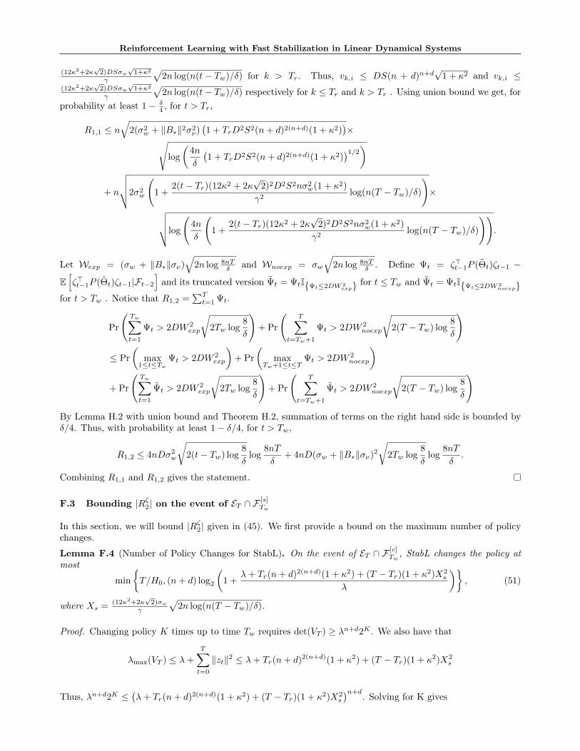
Reinforcement Learning with Fast Stabilization in Linear Dynamical Systems
(12κ2+2κ√2)DSσw
√1+κ2
γ
√2n log(n(t− Tw)/δ) for k > Tr. Thus, vk,i ≤ DS(n + d)n+d
√1 + κ2 and vk,i ≤
(12κ2+2κ√2)DSσw
√1+κ2
γ
√2n log(n(t− Tw)/δ) respectively for k ≤ Tr and k > Tr . Using union bound we get, for
probability at least 1− δ4 , for t > Tr,
R1,1 ≤ n√
2(σ2w + ∥B∗∥2σ2
ν)(1 + TrD2S2(n+ d)2(n+d)(1 + κ2)
)×√
log
(4n
δ
(1 + TrD2S2(n+ d)2(n+d)(1 + κ2)
)1/2)
+ n
√√√√2σ2w
(1 +
2(t− Tr)(12κ2 + 2κ√2)2D2S2nσ2
w(1 + κ2)
γ2log(n(T − Tw)/δ)
)×
√√√√log
(4n
δ
(1 +
2(t− Tr)(12κ2 + 2κ√2)2D2S2nσ2
w(1 + κ2)
γ2log(n(T − Tw)/δ)
)).
Let Wexp = (σw + ∥B∗∥σν)√2n log 8nT
δ and Wnoexp = σw
√2n log 8nT
δ . Define Ψt = ζ⊤t−1P (Θt)ζt−1 −
E[ζ⊤t−1P (Θt)ζt−1|Ft−2
]and its truncated version Ψt = ΨtIΨt≤2DW 2
exp for t ≤ Tw and Ψt = ΨtIΨt≤2DW 2noexp
for t > Tw . Notice that R1,2 =∑T
t=1 Ψt.
Pr
(Tw∑t=1
Ψt > 2DW 2exp
√2Tw log
8
δ
)+ Pr
(T∑
t=Tw+1
Ψt > 2DW 2noexp
√2(T − Tw) log
8
δ
)
≤ Pr
(max
1≤t≤Tw
Ψt > 2DW 2exp
)+ Pr
(max
Tw+1≤t≤TΨt > 2DW 2
noexp
)+ Pr
(Tw∑t=1
Ψt > 2DW 2exp
√2Tw log
8
δ
)+ Pr
(T∑
t=Tw+1
Ψt > 2DW 2noexp
√2(T − Tw) log
8
δ
)
By Lemma H.2 with union bound and Theorem H.2, summation of terms on the right hand side is bounded byδ/4. Thus, with probability at least 1− δ/4, for t > Tw,
R1,2 ≤ 4nDσ2w
√2(t− Tw) log
8
δlog
8nT
δ+ 4nD(σw + ∥B∗∥σν)
2
√2Tw log
8
δlog
8nT
δ.
Combining R1,1 and R1,2 gives the statement.
F.3 Bounding |Rζ2| on the event of ET ∩ F [s]
Tw
In this section, we will bound |Rζ2| given in (45). We first provide a bound on the maximum number of policy
changes.
Lemma F.4 (Number of Policy Changes for StabL). On the event of ET ∩ F [c]Tw
, StabL changes the policy atmost
min
T/H0, (n+ d) log2
(1 +
λ+ Tr(n+ d)2(n+d)(1 + κ2) + (T − Tr)(1 + κ2)X2s
λ
), (51)
where Xs =(12κ2+2κ
√2)σw
γ
√2n log(n(T − Tw)/δ).
Proof. Changing policy K times up to time Tw requires det(VT ) ≥ λn+d2K . We also have that
λmax(VT ) ≤ λ+
T∑t=0
∥zt∥2 ≤ λ+ Tr(n+ d)2(n+d)(1 + κ2) + (T − Tr)(1 + κ2)X2s
Thus, λn+d2K ≤(λ+ Tr(n+ d)2(n+d)(1 + κ2) + (T − Tr)(1 + κ2)X2
s
)n+d. Solving for K gives

Sahin Lale, Kamyar Azizzadenesheli, Babak Hassibi, Anima Anandkumar
K ≤ (n+ d) log2
(1 +
Tr(n+ d)2(n+d)(1 + κ2) + (T − Tr)(1 + κ2)X2s
λ
).
Moreover, the number of policy changes is also controlled by the lower bound H0 on the duration of eachcontroller. This policy update method would give at most T/H0 policy changes. Since for the policy updateof StabL requires both conditions to be met, the upper bound on the number of policy changes is minimum ofthese.
Notice that besides the policy change instances, all the terms in Rζ2 are 0. Therefore, we have the following
results for stabilizable systems.
Lemma F.5 (Bounding Rζ2 for StabL). Let Rζ
2 be as defined by (45). Under the event of ET ∩F [s]Tw
, using StabL,we have
|Rζ2| ≤ 2D(n+ d)2(n+d)+1 log2
(1 +
Tr(n+ d)2(n+d)(1 + κ2)
λ
)+ 2DX2
s (n+ d) log2
(1 +
Tr(n+ d)2(n+d)(1 + κ2) + (T − Tr)(1 + κ2)X2s
λ
)
where Xs =(12κ2+2κ
√2)σw
γ
√2n log(n(T − Tw)/δ)
Proof. On the event ET ∩ F [s]Tw
, we know the maximum number of policy changes up to Tr and T using Lemma
F.4. Using the fact that ∥xt∥ ≤ (n+d)n+d for t ≤ Tr and ∥xt∥ ≤ (12κ2+2κ√2)σw
γ
√2n log(n(t− Tw)/δ), we obtain
the statement of the lemma.
F.4 Bounding |Rζ3| on the event of ET ∩ F [s]
Tw
Before bounding Rζ3, first consider the following for stabilizable LQRs.
Lemma F.6. On the event of ET ∩ F [s]Tw
, using StabL in a stabilizable LQR, the following holds,
T∑t=0
∥(Θ∗ − Θt)⊤zt∥2≤
8(1 + κ2)β2T (δ)
λ×(
(n+ d)2(n+d) max
2,
(1 +
(1 + κ2)(n+ d)2(n+d)
λ
)H0log
det(VTr)
det(λI)
+X2s max
2,
(1 +
(1 + κ2)X2s
λ
)H0log
det(VT )
det(VTr)
)
where Xs =(12κ2+2κ
√2)σw
γ
√2n log(n(t− Tw)/δ).
Proof. Let st = (Θ∗ − Θt)⊤zt and τ ≤ t be the time step that the last policy change happened. We have the
following using triangle inequality,
∥st∥ ≤ ∥(Θ∗ − Θt)⊤zt∥+ ∥(Θt − Θt)
⊤zt∥.

Reinforcement Learning with Fast Stabilization in Linear Dynamical Systems
For all Θ ∈ Cτ (δ), for τ ≤ Tr, we have
∥(Θ− Θt)⊤zt∥ ≤ ∥V 1/2
t (Θ− Θt)∥∥zt∥V −1t
(52)
≤ ∥V 1/2τ (Θ− Θt)∥
√det(Vt)
det(Vτ )∥zt∥V −1
t(53)
≤ max
√2,
√(1 +
(1 + κ2)(n+ d)2(n+d)
λ
)H0
∥V 1/2τ (Θ− Θt)∥∥zt∥V −1
t(54)
≤ max
√2,
√(1 +
(1 + κ2)(n+ d)2(n+d)
λ
)H0
βτ (δ)∥zt∥V −1t
. (55)
Similarly, for for all Θ ∈ Cτ (δ), for τ > Tr, we have
∥(Θ− Θt)⊤zt∥ ≤ max
√2,
√(1 +
(1 + κ2)X2s
λ
)H0
βτ (δ)∥zt∥V −1t
Using these results, we obtain,
T∑t=0
∥(Θ∗ − Θt)⊤zt∥2
≤ 8max
2,
(1 +
(1 + κ2)(n+ d)2(n+d)
λ
)H0
β2T (δ)(1 + κ2)(n+ d)2(n+d)
λlog
(det(VTr
)
det(λI)
)
+ 8max
2,
(1 +
(1 + κ2)X2s
λ
)H0
β2T (δ)(1 + κ2)X2
s
λlog
(det(VT )
det(VTr)
)
where we use Lemma H.1.
Using Lemma F.6, we bound Rζ3 as follows.
Lemma F.7 (Bounding Rζ3 for StabL). Let Rζ
3 be as defined by (46). Under the event of ET ∩F [s]Tw
, using StabLwith the choice of λ = (1 + κ2)X2
s , we have
|Rζ3| = O
((n+ d)(H0+2)(n+d)+2
√n√
Tr + (n+ d)n√T − Tr
)
Proof. Let Y1 =8(1+κ2)β2
T (δ)λ (n + d)2(n+d) max
2,(1 + (1+κ2)(n+d)2(n+d)
λ
)H0log
det(VTr )det(λI) and Y2 =
8(1+κ2)β2T (δ)
λ X2s max
2,(1 +
(1+κ2)X2s
λ
)H0log det(VT )
det(VTr )for Xs = (12κ2+2κ
√2)σw
γ
√2n log(n(t− Tw)/δ). The fol-
lowing uses triangle inequality and Cauchy Schwarz inequality and again triangle inequality to give:

Sahin Lale, Kamyar Azizzadenesheli, Babak Hassibi, Anima Anandkumar
∣∣∣Rζ3
∣∣∣ ≤ T∑t=0
∣∣∣∣∥∥∥P (Θt)1/2Θ⊤
t zt
∥∥∥2 − ∥∥∥P (Θt)1/2Θ⊤
∗ zt
∥∥∥2∣∣∣∣=
Tr∑t=0
∣∣∣∣∥∥∥P (Θt)1/2Θ⊤
t zt
∥∥∥2 − ∥∥∥P (Θt)1/2Θ⊤
∗ zt
∥∥∥2∣∣∣∣+ T∑t=Tr
∣∣∣∣∥∥∥P (Θt)1/2Θ⊤
t zt
∥∥∥2 − ∥∥∥P (Θt)1/2Θ⊤
∗ zt
∥∥∥2∣∣∣∣≤
(Tr∑t=0
(∥∥∥P (Θt)1/2Θ⊤
t zt
∥∥∥−∥∥∥P (Θt)1/2Θ⊤
∗ zt
∥∥∥)2)1/2( Tr∑t=0
(∥∥∥P (Θt)1/2Θ⊤
t zt
∥∥∥+∥∥∥P (Θt)1/2Θ⊤
∗ zt
∥∥∥)2)1/2
+
(T∑
t=Tr
(∥∥∥P (Θt)1/2Θ⊤
t zt
∥∥∥−∥∥∥P (Θt)1/2Θ⊤
∗ zt
∥∥∥)2)1/2( T∑t=Tr
(∥∥∥P (Θt)1/2Θ⊤
t zt
∥∥∥+∥∥∥P (Θt)1/2Θ⊤
∗ zt
∥∥∥)2)1/2
≤
(Tr∑t=0
∥∥∥∥P (Θt)1/2(Θt −Θ∗
)⊤zt
∥∥∥∥2)1/2( Tr∑
t=0
(∥∥∥P (Θt)1/2Θ⊤
t zt
∥∥∥+ ∥∥∥P (Θt)1/2Θ⊤
∗ zt
∥∥∥)2)1/2
+
(T∑
t=Tr
∥∥∥∥P (Θt)1/2(Θt −Θ∗
)⊤zt
∥∥∥∥2)1/2( T∑
t=Tr
(∥∥∥P (Θt)1/2Θ⊤
t zt
∥∥∥+ ∥∥∥P (Θt)1/2Θ⊤
∗ zt
∥∥∥)2)1/2
≤√
Y1
√4TrD(1 + κ2)S2(n+ d)2(n+d) +
√Y2
√4(T − Tr)D(1 + κ2)S2X2
s
≤max
8, 4
√2(1 + (1+κ2)(n+d)2(n+d)
λ
)H0/2DS(1 + κ2)βT (δ)(n+ d)2(n+d)
√λ
×√Tr(n+ d) log
(1 +
Tr(1 + κ2)(n+ d)2(n+d)
λ(n+ d)
)
+
max
8, 4
√2(1 +
(1+κ2)X2s
λ
)H0/2DS(1 + κ2)βT (δ)
√λ
X2s×√
(T − Tr)(n+ d) log
(1 +
Tr(1 + κ2)(n+ d)2(n+d) + (T − Tr)X2s
λ(n+ d)
)
Examining the first term, it has the dimension dependency of (n+d)(n+d)H0×√n(n+ d)×(n+d)2(n+d)×
√n+ d
where√n(n+ d) is due to βT (δ). For the second term, with the choice of λ = (1 + κ2)X2
s , the exponential
dependency on the dimension with H0 can be converted to a scalar multiplier, i.e.,(1 +
(1+κ2)X2s
λ
)H0/2
=√2H0
and (1 + κ2)X2s/
√λ =
√(1 + κ2)Xs. Therefore, for the second term, we have the dimension dependency of√
n(n+ d)×√n×
√n+ d which gives the advertised bound.
F.5 Combining Terms for Final Regret Upper Bound
Proof of Theorem 4.2: Recall that
REGRET(T ) ≤ σ2νTwD∥B∗∥2F +
Tw∑t=0
(2ν⊤t Rut + ν⊤t Rνt
)+Rζ
1 −Rζ2 −Rζ
3.
Combining Lemma F.1 for∑Tw
t=0
(2ν⊤t Rut + ν⊤t Rνt
), Lemma F.3 for Rζ
1, Lemma F.5 for |Rζ2| and Lemma F.7
for |Rζ3|, we get the advertised regret bound.

Reinforcement Learning with Fast Stabilization in Linear Dynamical Systems
G CONTROLLABILITY ASSUMPTION IN ABBASI-YADKORI ANDSZEPESVARI (2011)
In Abbasi-Yadkori and Szepesvári (2011), the authors derive their results for the following setting:Assumption G.1 (Controllable Linear Dynamical System). The unknown parameter Θ∗ is a member of a setSc such that
Sc ⊆Θ′ = [A′, B′] ∈ Rn×(n+d)
∣∣ Θ′ is controllable, ∥A′ +B′K(Θ′)∥ ≤ Υ < 1, ∥Θ′∥F ≤ S
Following the controllability and the boundedness of Sc, we have finite numbers D and κ ≥ 1 s.t.,sup∥P (Θ′)∥ | Θ′ ∈ Sc ≤ D and sup∥K(Θ′)∥ | Θ′ ∈ Sc ≤ κ.
Our results are strict generalizations of these since stabilizable systems subsume controllable systems and allclosed-loop contractible systems considered with Assumption G.1 is a subset of general stable closed-loop systemsconsidered in this work. For the setting in Assumption G.1, we can bound the state following similar steps tostabilizable case but since the closed-loop system is contractible we do not need minimum length on epochof an optimistic controller since the state would always shrink. Adopting the proofs provided in this work toAssumption G.1, one can obtain the similar polynomial dimension dependency via additional exploration ofStabL. This shows that with additional exploration the result of Abbasi-Yadkori and Szepesvári (2011) could bedirectly improved.
H TECHNICAL THEOREMS AND LEMMAS
Theorem H.1 (Self-normalized bound for vector-valued martingales (Abbasi-Yadkori et al., 2011)). Let (Ft; k ≥0) be a filtration, (mk; k ≥ 0) be an Rd-valued stochastic process adapted to (Fk) , (ηk; k ≥ 1) be a real-valuedmartingale difference process adapted to (Fk) . Assume that ηk is conditionally sub-Gaussian with constant R.Consider the martingale
St =∑t
k=1ηkmk−1
and the matrix-valued processes
Vt =∑t
k=1mk−1m
⊤k−1, V t = V + Vt, t ≥ 0
Then for any 0 < δ < 1, with probability 1− δ
∀t ≥ 0, ∥St∥2V −1t
≤ 2R2 log
(det(V t
)1/2det(V )−1/2
δ
)Theorem H.2 (Azuma’s inequality). Assume that (Xs; s ≥ 0) is a supermartingale and |Xs −Xs−1| ≤ cs almostsurely. Then for all t > 0 and all ϵ > 0,
P (|Xt −X0| ≥ ϵ) ≤ 2 exp
(−ϵ2
2∑t
s=1 c2s
)Lemma H.1 (Bound on Logarithm of the Determinant of Sample Covariance Matrix (Abbasi-Yadkori et al.,2011)). The following holds for any t ≥ 1 :
t−1∑k=0
(∥zk∥2V −1
k∧ 1)≤ 2 log
det (Vt)
det(λI)
Further, when the covariates satisfy ∥zt∥ ≤ cm, t ≥ 0 with some cm > 0 w.p. 1 then
logdet (Vt)
det(λI)≤ (n+ d) log
(λ(n+ d) + tc2m
λ(n+ d)
)Lemma H.2 (Norm of Subgaussian vector). Let v ∈ Rd be a entry-wise R-subgaussian random variable. Thenwith probability 1− δ, ∥v∥ ≤ R
√2d log(d/δ).

Sahin Lale, Kamyar Azizzadenesheli, Babak Hassibi, Anima Anandkumar
I IMPLEMENTATION DETAILS OF EXPERIMENTS AND ADDITIONALRESULTS
In this section, we provide the simulation setups, with the parameter settings for each algorithm and the de-tails of the adaptive control tasks. The implementations and further system considerations are available athttps://github.com/SahinLale/StabL. In the experiments, we use four adaptive control tasks:
(1) A marginally unstable Laplacian system (Dean et al., 2018)
(2) The longitudinal flight control of Boeing 747 with linearized dynamics (Ishihara et al., 1992)
(3) Unmanned aerial vehicle (UAV) that operates in a 2-D plane (Zhao et al., 2021)
(4) A stabilizable but not controllable linear dynamical system.
For each setting we deploy 4 different algorithms:
(i) Our algorithm StabL,
(ii) OFULQ of Abbasi-Yadkori and Szepesvári (2011),
(iii) Certainty equivalent controller (CEC) with fixed isotropic perturbations,
(iv) CEC with decaying isotropic perturbations.
For each algorithm there are different varying parameters. For each adaptive control task, we tune each parameterin terms of regret performance and present the performance of the best performing parameter choices since theregret analysis for each algorithm considers the worst case scenario. In each setting, we will specify theseparameters choices for each algorithm. We use the actual errors ∥Θt − Θ∗∥2 rather than bounds or bootstrapestimates for each algorithm, since we observe that the overall effect is negligible as mentioned in Dean et al.(2018). The following gives the implementation details of each algorithm.
(i) StabL We have σν , H0 and Tw as the varying parameters. In the implementation of optimistic parametersearch we deploy projected gradient descent (PGD), which works efficiently for the small dimensional problems.The implementation follows Section G.1 of (Dean et al., 2018). Note that this approach, hence the optimisticparameter choice, can be computationally challenging for higher dimensional systems. We pick the regularizerλ = 0.05 for all adaptive control tasks.
(ii) OFULQ We deploy a slight modification on the implementation of OFULQ given by (Abbasi-Yadkori andSzepesvári, 2011). Similar to StabL, we add an additional minimum policy duration constraint to the generalswitching constraints of OFULQ, i.e., the standard determinant doubling of Vt. This prevents too frequentchanges in the beginning of the algorithm and dramatically improves the regret performance. This minimumduration HOFU
0 is the only varying parameter for OFULQ. For the optimistic parameter search we also implementPGD. We pick the regularizer λ = 0.001 for all adaptive control tasks.
(iii) CEC w/t fixed perturbations This algorithm is the standard baseline in control theory. In theimplementation, the optimal infinite-horizon LQR controller for the estimated system is deployed and fixedisotropic perturbations N (0, σ2
expI) are injected throughout the implementation. The isotropic perturbations areinjected since it is well-known that certainty equivalent controllers can result with drastically incorrect parameterestimates (Lai et al., 1982; Becker et al., 1985; Kumar, 1990) due to lack of exploration. The policy changeshappen in epochs with linear scaling, i.e., each epoch i is of iHep length. This growth is observed to be preferableover the standard exponentially increasing epoch lengths adopted in theoretical analyses of the worst case regretguarantees. Thus, the varying parameters for CEC w/t fixed perturbations are σexp and Hep. We pick theregularizer λ = 0.5 for all adaptive control tasks.

Reinforcement Learning with Fast Stabilization in Linear Dynamical Systems
(iv) CEC w/t decaying perturbations The implementation of this algorithm is similar to (iii). Thedifference is that the injected perturbations have decaying variance over epochs. We adopt the decay of 1/
√i
for each epoch i, i.e. σi,exp = σdecexp/
√i for some initial σdec
exp such that isotropic perturbations are injected ineach epoch. Based on the extensive experimental study, we deduced that this decay performs better than thedecay of i−1/3 as given in Dean et al. (2018) or 2−i/2 as given in Simchowitz and Foster (2020). The varyingparameters for this algorithm are σdec
exp and Hdecep in which the latter defines the first epoch length in the linear
scaling of epochs. We pick the regularizer λ = 0.05 for all adaptive control tasks.
In each experiment, the system starts from x0 = 0 to reduce variance over runs. For each setting, we run 200independent runs with the duration of 200 time steps. Note that we do not compare StabL with the adaptivecontrol algorithms provided in (Simchowitz and Foster, 2020; Simchowitz et al., 2020; Dean et al., 2018; Cohenet al., 2019; Faradonbeh et al., 2018b, 2020) which all require a given initial stabilizing policy or stable open-loopdynamics and (Abeille and Lazaric, 2017) which is tailored for scalar systems. Moreover, Chen and Hazan (2020)deals with adversarial LQR setting and uses “significantly” large inputs to identify the model dynamics whichcauses orders of magnitude worse regret.
I.1 Marginally Unstable Laplacian System
The LQR problem is given as
A∗ =
1.01 0.01 00.01 1.01 0.010 0.01 1.01
, B∗ = I3×3, Q = 10I, R = I, w ∼ N (0, I). (56)
This system dynamics have been studied in (Dean et al., 2018, 2019; Abbasi-Yadkori et al., 2018; Tu and Recht,2018) and it corresponds a Laplacian system with weakly connected adjacent nodes. Notice that the inputs haveless cost weight than the states. This skewed cost combined with the unstable dynamics severely hinders thedesign of effective strategies for OFU-based methods.
Algorithmic Setups: For StabL, we set H0 = 15, Tw = 35 and σν = 1.5. For CEC with decaying perturbation,we set Hdec
ep = 20, and σdecexp = 2. For CEC with fixed perturbation, we set σexp = 1.3 and Hep = 15. For OFULQ,
we set HOFU0 = 6.
Regret After 200 Time Steps: In Table 6, we provide the regret performance of the algorithms after 200time steps of adaptive control in the Laplacian system. As expected the regret performance of OFULQ suffersthe most regret due to unstable dynamics and skewed cost, which makes it difficult to design effective policiesfor the OFU-based algorithms. Even though StabL uses OFU principle, it overcomes the difficulty to designeffective policies via the improved exploration in the early stages and achieves the best regret performance.
Table 6: Regret After 200 Time Steps in Marginally Unstable Laplacian System
Algorithm Average Regret Best 95% Best 90% Best 75% Best 50%StabL 1.55× 10⁴ 1.42× 10⁴ 1.32× 10⁴ 1.12× 10⁴ 8.89× 10³
OFULQ 6.17× 10¹⁰ 4.57× 10⁷ 4.01× 10⁶ 3.49× 10⁵ 4.70× 10⁴
CEC w/t Fixed 3.72× 10¹⁰ 2.23× 10⁵ 2.14× 10⁴ 1.95× 10⁴ 1.73× 10⁴
CEC w/t Decay 4.63× 10⁴ 4.27× 10⁴ 4.03× 10⁴ 3.51× 10⁴ 2.84× 10⁴
Figure 3 gives the regret comparison between StabL and CEC with decaying isotropic perturbations whichperforms the second best in the given Laplacian system. Note that we did not include OFULQ and CEC w/tfixed perturbations in the figure since they perform orders of magnitude worse that StabL and CEC w/t decayingperturbations.
Maximum State Norm: In Table 7, we display the stabilization capabilities of the algorithms by providingthe averages of the maximum ℓ2 norms of the states in 200 independent runs. We also include the worst casestate magnitudes which demonstrates how controlled the states are during the entire adaptive control task. Theresults show that StabL maintains the smallest magnitude of the state and thus, the most stable dynamics.We also verify that after the first policy change which happens after 15 time steps, the spectral radius of theclosed-loop system formed via StabL is always stable, i.e. ρ(A∗ +B∗K(Θt)) < 1 for t > 15.
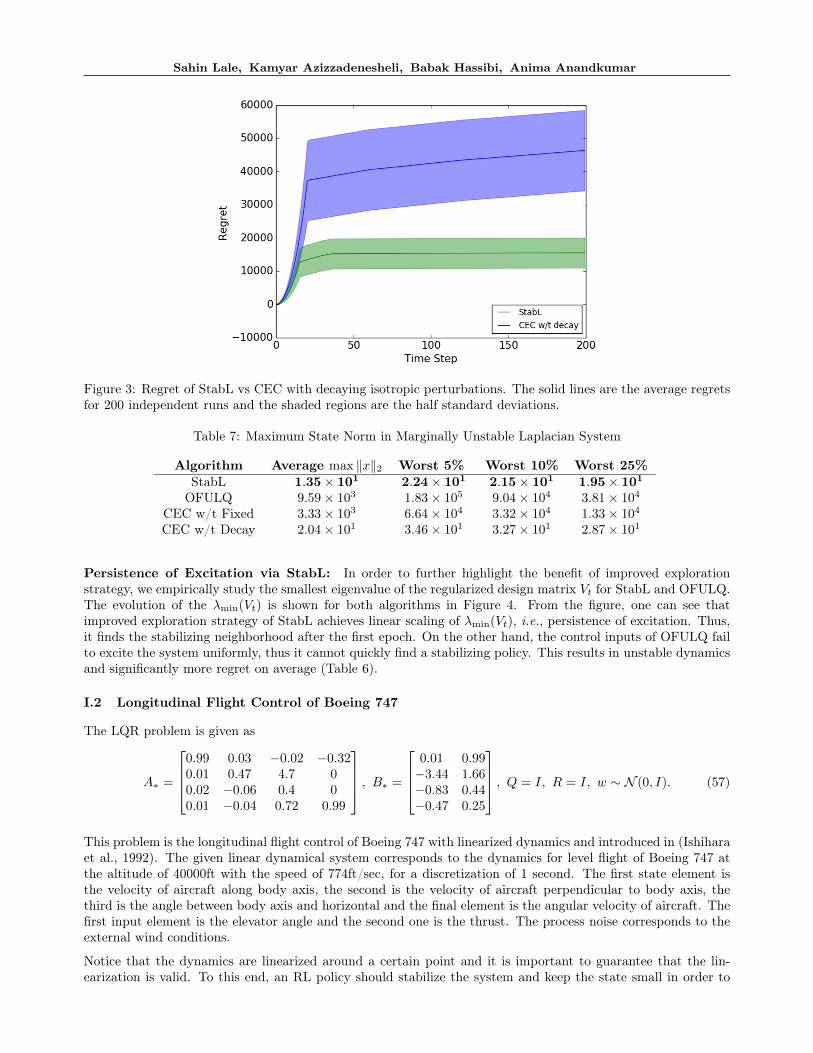
Sahin Lale, Kamyar Azizzadenesheli, Babak Hassibi, Anima Anandkumar
Figure 3: Regret of StabL vs CEC with decaying isotropic perturbations. The solid lines are the average regretsfor 200 independent runs and the shaded regions are the half standard deviations.
Table 7: Maximum State Norm in Marginally Unstable Laplacian System
Algorithm Average max ∥x∥2 Worst 5% Worst 10% Worst 25%StabL 1.35× 101 2.24× 101 2.15× 101 1.95× 101
OFULQ 9.59× 10³ 1.83× 10⁵ 9.04× 10⁴ 3.81× 10⁴
CEC w/t Fixed 3.33× 10³ 6.64× 10⁴ 3.32× 10⁴ 1.33× 10⁴
CEC w/t Decay 2.04× 101 3.46× 101 3.27× 101 2.87× 101
Persistence of Excitation via StabL: In order to further highlight the benefit of improved explorationstrategy, we empirically study the smallest eigenvalue of the regularized design matrix Vt for StabL and OFULQ.The evolution of the λmin(Vt) is shown for both algorithms in Figure 4. From the figure, one can see thatimproved exploration strategy of StabL achieves linear scaling of λmin(Vt), i.e., persistence of excitation. Thus,it finds the stabilizing neighborhood after the first epoch. On the other hand, the control inputs of OFULQ failto excite the system uniformly, thus it cannot quickly find a stabilizing policy. This results in unstable dynamicsand significantly more regret on average (Table 6).
I.2 Longitudinal Flight Control of Boeing 747
The LQR problem is given as
A∗ =
0.99 0.03 −0.02 −0.320.01 0.47 4.7 00.02 −0.06 0.4 00.01 −0.04 0.72 0.99
, B∗ =
0.01 0.99−3.44 1.66−0.83 0.44−0.47 0.25
, Q = I, R = I, w ∼ N (0, I). (57)
This problem is the longitudinal flight control of Boeing 747 with linearized dynamics and introduced in (Ishiharaet al., 1992). The given linear dynamical system corresponds to the dynamics for level flight of Boeing 747 atthe altitude of 40000ft with the speed of 774ft/sec, for a discretization of 1 second. The first state element isthe velocity of aircraft along body axis, the second is the velocity of aircraft perpendicular to body axis, thethird is the angle between body axis and horizontal and the final element is the angular velocity of aircraft. Thefirst input element is the elevator angle and the second one is the thrust. The process noise corresponds to theexternal wind conditions.
Notice that the dynamics are linearized around a certain point and it is important to guarantee that the lin-earization is valid. To this end, an RL policy should stabilize the system and keep the state small in order to
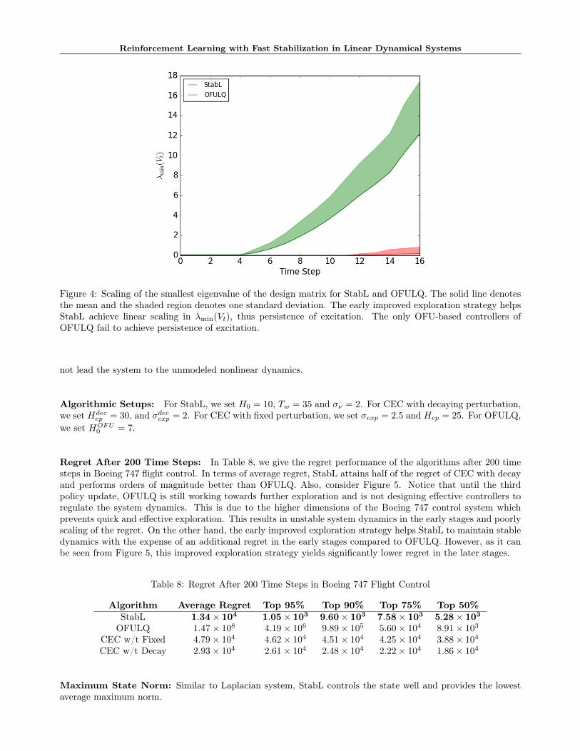
Reinforcement Learning with Fast Stabilization in Linear Dynamical Systems
Figure 4: Scaling of the smallest eigenvalue of the design matrix for StabL and OFULQ. The solid line denotesthe mean and the shaded region denotes one standard deviation. The early improved exploration strategy helpsStabL achieve linear scaling in λmin(Vt), thus persistence of excitation. The only OFU-based controllers ofOFULQ fail to achieve persistence of excitation.
not lead the system to the unmodeled nonlinear dynamics.
Algorithmic Setups: For StabL, we set H0 = 10, Tw = 35 and σν = 2. For CEC with decaying perturbation,we set Hdec
ep = 30, and σdecexp = 2. For CEC with fixed perturbation, we set σexp = 2.5 and Hep = 25. For OFULQ,
we set HOFU0 = 7.
Regret After 200 Time Steps: In Table 8, we give the regret performance of the algorithms after 200 timesteps in Boeing 747 flight control. In terms of average regret, StabL attains half of the regret of CEC with decayand performs orders of magnitude better than OFULQ. Also, consider Figure 5. Notice that until the thirdpolicy update, OFULQ is still working towards further exploration and is not designing effective controllers toregulate the system dynamics. This is due to the higher dimensions of the Boeing 747 control system whichprevents quick and effective exploration. This results in unstable system dynamics in the early stages and poorlyscaling of the regret. On the other hand, the early improved exploration strategy helps StabL to maintain stabledynamics with the expense of an additional regret in the early stages compared to OFULQ. However, as it canbe seen from Figure 5, this improved exploration strategy yields significantly lower regret in the later stages.
Table 8: Regret After 200 Time Steps in Boeing 747 Flight Control
Algorithm Average Regret Top 95% Top 90% Top 75% Top 50%StabL 1.34× 10⁴ 1.05× 10³ 9.60× 10³ 7.58× 10³ 5.28× 10³
OFULQ 1.47× 10⁸ 4.19× 10⁶ 9.89× 10⁵ 5.60× 10⁴ 8.91× 10³
CEC w/t Fixed 4.79× 10⁴ 4.62× 10⁴ 4.51× 10⁴ 4.25× 10⁴ 3.88× 10⁴
CEC w/t Decay 2.93× 10⁴ 2.61× 10⁴ 2.48× 10⁴ 2.22× 10⁴ 1.86× 10⁴
Maximum State Norm: Similar to Laplacian system, StabL controls the state well and provides the lowestaverage maximum norm.

Sahin Lale, Kamyar Azizzadenesheli, Babak Hassibi, Anima Anandkumar
Figure 5: Regret Comparison of all algorithms in Boeing 747 flight control. The solid lines are the average regretsfor 200 independent runs and the shaded regions are the quarter standard deviations.
Table 9: Maximum State Norm in Boeing 747 Control
Algorithm Average max ∥x∥2 Worst 5% Worst 10% Worst 25%StabL 3.38× 101 8.02× 101 7.01× 101 5.23× 101
OFULQ 1.62× 10³ 2.25× 10⁴ 1.37× 10⁴ 6.26× 10³
CEC w/t Fixed 4.97× 101 7.78× 101 7.31× 101 6.48× 101
CEC w/t Decay 4.60× 101 7.96× 101 7.25× 101 6.31× 101
I.3 Unmanned Aerial Vehicle (UAV) in 2-D plane
The LQR problem is given as
A∗ =
1 0.5 0 00 1 0 00 0 1 0.50 0 0 1
, B∗ =
0.125 00.5 00 0.1250 0.5
, Q = diag(1, 0.1, 2, 0.2), R = I, w ∼ N (0, I) (58)
This problem is the linearized model of a UAV which operates in a 2-D plane (Zhao et al., 2021). Notice thatit corresponds to the model of double integrator. The first and third state elements correspond to the position,whereas the second and fourth state elements are velocity components. The inputs are the acceleration. Theprocess noise corresponds to the external wind conditions. Similar to Boeing 747, the dynamics are linearizedand keeping the state vector small is critical in order to maintain the validity of the linearization.
Algorithmic Setups: For StabL, we set H0 = 20, Tw = 55 and σν = 4. For CEC with decaying perturbation,we set Hdec
ep = 30, and σdecexp = 3.5. For CEC with fixed perturbation, we set σexp = 3 and Hep = 35. For OFULQ,
we set HOFU0 = 7.
Regret After 200 Time Steps: In Table 10, we give the regret performance of the algorithms after 200 timesteps in UAV control control task. Once more, StabL performs significantly better than other RL methods. Theevolution of the average regret is also given in Figure 6. As suggested by the theory, by paying a linear regret costfor a short period of time in the early stages, StabL guarantees stabilizing the underlying system and achievesthe best regret performance.

Reinforcement Learning with Fast Stabilization in Linear Dynamical Systems
Table 10: Regret After 200 Time Steps in UAV Control
Algorithm Average Regret Top 95% Top 90% Top 75% Top 50%StabL 1.53× 10⁵ 1.05× 10⁵ 9.23× 10⁴ 6.85× 10⁴ 4.47× 10⁴
OFULQ 5.06× 10⁷ 1.75× 10⁶ 1.03× 10⁶ 2.46× 10⁵ 5.82× 10⁴
CEC w/t Fixed 4.52× 10⁵ 3.80× 10⁵ 3.35× 10⁵ 2.50× 10⁵ 1.64× 10⁵
CEC w/t Decay 3.24× 10⁵ 2.70× 10⁵ 2.37× 10⁵ 1.75× 10⁵ 1.03× 10⁵
Maximum State Norm:
Table 11: Maximum State Norm in UAV Control
Algorithm Average max ∥x∥2 Worst 5% Worst 10% Worst 25%StabL 8.46× 101 2.51× 10² 2.00× 10² 1.50× 10²
OFULQ 5.61× 10² 6.35× 10³ 3.78× 10³ 1.90× 10³
CEC w/t Fixed 1.45× 10² 3.12× 10² 2.91× 10² 2.42× 10²
CEC w/t Decay 1.26× 10² 2.71× 10² 2.48× 10² 2.12× 10²
Figure 6: Regret Comparison of all algorithms in UAV control task. The solid lines are the average regrets for200 independent runs and the shaded regions are the quarter standard deviations.
I.4 Stabilizable but Not Controllable System
The LQR problem is given as
A∗ =
−2 0 1.11.5 0.9 1.30 0 0.5
, B∗ =
1 00 10 0
, Q = I, R = I, w ∼ N (0, I) (59)
This problem is particularly challenging in terms of system identification and controller design since the system isnot controllable but stabilizable. As expected besides StabL which is tailored for the general stabilizable setting,other algorithms perform poorly. In fact, CEC with fixed noise significantly blows up due to significantly unstabledynamics for the controllable part of the system. Therefore, we only present the remaining three algorithms.
Algorithmic Setups: For StabL, we set H0 = 8, Tw = 20 and σν = 2.5. For CEC with decaying perturbation,we set Hdec
ep = 30, and σdecexp = 3. For OFULQ, we set HOFU
0 = 6.

Sahin Lale, Kamyar Azizzadenesheli, Babak Hassibi, Anima Anandkumar
Regret After 200 Time Steps: Table 12 provides the regret of the algorithms after 200 time steps. Thissetting is where OFULQ fails dramatically due to not being tailored for the stabilizable systems. Compared toCEC with decaying perturbation, StabL also provides an order of magnitude improvement (Figure 7)
Table 12: Regret After 200 Time Steps in Stabilizable but Not Controllable System (59)
Algorithm Average Regret Top 95% Top 90% Top 75% Top 50%StabL 1.68× 10⁶ 9.56× 10⁵ 7.21× 10⁵ 3.72× 10⁵ 1.29× 10⁵
OFULQ 5.20× 10¹² 1.74× 10¹² 8.27× 10¹¹ 2.13× 10¹¹ 4.51× 10¹⁰
CEC w/t Decay 1.56× 10⁷ 1.17× 10⁷ 9.75× 10⁶ 5.96× 10⁶ 2.33× 10⁶
Figure 7: Regret Comparison of three algorithms in controlling (59). The solid lines are the average regrets for200 independent runs and the shaded regions are the quarter standard deviations.
Maximum State Norm:
Table 13: Maximum State Norm in the Control of Stabilizable but Not Controllable System (59)
Algorithm Average max ∥x∥2 Worst 5% Worst 10% Worst 25%StabL 3.02× 10² 1.04× 10³ 8.88× 10² 6.68× 10²
OFULQ 4.39× 10⁵ 3.10× 10⁶ 2.40× 10⁶ 1.39× 10⁶
CEC w/t Decay 1.37× 10³ 4.07× 10³ 3.54× 10³ 2.78× 10³
Related Documents