Reinforcement Learning Policy Gradient Marcello Restelli March–April, 2015

Welcome message from author
This document is posted to help you gain knowledge. Please leave a comment to let me know what you think about it! Share it to your friends and learn new things together.
Transcript

Reinforcement LearningPolicy Gradient
Marcello Restelli
March–April, 2015

MarcelloRestelli
Black–BoxApproaches
White–BoxApproachesMonte–Carlo PolicyGradient
Actor–Critic PolicyGradient
Value Based and Policy–Based ReinforcementLearning
Value BasedLearn value functionImplicit policy
Policy BasedNo value functionLearn policy
Actor–CriticLearn value functionLearn policy

MarcelloRestelli
Black–BoxApproaches
White–BoxApproachesMonte–Carlo PolicyGradient
Actor–Critic PolicyGradient
Advantages of Policy–Based RL
Advantages:Better convergence propertiesEffective in high–dimensional or continuous actionspacesCan benefit from demonstrationsPolicy subspace can be chosen according to the taskExploration can be directly controlledCan learn stochastic policies
Disadvantages:Typically converge to a local rather than a globaloptimumEvaluating a policy is typically inefficient and highvariance

MarcelloRestelli
Black–BoxApproaches
White–BoxApproachesMonte–Carlo PolicyGradient
Actor–Critic PolicyGradient
Example: Rock–Paper–Scissor
Two–player game of rock–paper–scissorsScissors beats paperRock beats scissorsPaper beats rock
Consider policies for iterated rock–paper–scissorsA deterministic policy is easily exploitedA uniform random policy is optimal (i.e., Nashequilibrium)

MarcelloRestelli
Black–BoxApproaches
White–BoxApproachesMonte–Carlo PolicyGradient
Actor–Critic PolicyGradient
Example: Aliased Gridworld
The agent cannot differentiate the gray statesConsider features of the following form (for all N, E, S,W)
φ(s,a) = 1(wall to N,a = move E)
Compare value–based RL, using an approximatevalue function
Qθ(s,a) = f (φ(s,a), θ)
To policy–based RL, using a parameterized policy
πθ(s,a) = g(φ(s,a), θ)

MarcelloRestelli
Black–BoxApproaches
White–BoxApproachesMonte–Carlo PolicyGradient
Actor–Critic PolicyGradient
Example: Aliased Gridworld
Under aliasing, an optimal deterministic policy willeither
move W in both gray statesmove E in both gray states
Either way, it can get stuck and never reach the moneyValue–based RL learns a near–deterministic policySo it will traverse the corridor for a long time
MarcelloRestelli
Black–BoxApproaches
White–BoxApproachesMonte–Carlo PolicyGradient
Actor–Critic PolicyGradient
Example: Aliased Gridworld
An optimal stochastic policy will randomly move E orW in gray states
πθ(wall to N and S, move E) = 0.5
πθ(wall to N and S, move W) = 0.5
It will reach the goal state in a few steps with highprobabilityPolicy–based RL can learn the optimal stochastic policy

MarcelloRestelli
Black–BoxApproaches
White–BoxApproachesMonte–Carlo PolicyGradient
Actor–Critic PolicyGradient
Policy Objective Function
Goal: given a policy πθ(a|s) with parameters θ, findbest θBut how do we measure the quality of a policy πθ?We want to optimize the expected return
J(θ) =
∫Sµ(s)Vπθ(s)ds =
∫S
dπθ(s)
∫Aπ(a|s)R(s,a)dads
where dπθ is the stationary distribution

MarcelloRestelli
Black–BoxApproaches
White–BoxApproachesMonte–Carlo PolicyGradient
Actor–Critic PolicyGradient
Policy Optimization
Policy based reinforcement learning is an optimizationproblemFind θ that maximizes J(θ)
Some approaches do not use gradientHill climbingSimplexGenetic algorithms
Greater efficiency often possible using gradientGradient descentConjugate gradientQuasi–Newton
We focus on gradient descent, many extensionspossibleAnd on methods that exploit sequential structure

MarcelloRestelli
Black–BoxApproaches
White–BoxApproachesMonte–Carlo PolicyGradient
Actor–Critic PolicyGradient
Greedy vs Incremental
Greedy updates
θπ′ = arg maxθ
Eπθ [Qπ(s,a)]
Vπ0
smallchange−−−−→ π1
largechange−−−−→ Vπ1
largechange−−−−→ π2
largechange−−−−→
Potentially unstable learning process with large policyjumpsPolicy Gradient updates
θπ′ = θπ + αdJ(θ)
dθ
∣∣∣∣θ=θπ
Vπ0
smallchange−−−−→ π1
smallchange−−−−→ Vπ1
smallchange−−−−→ π2
smallchange−−−−→
Stable learning process with smooth policyimprovement

MarcelloRestelli
Black–BoxApproaches
White–BoxApproachesMonte–Carlo PolicyGradient
Actor–Critic PolicyGradient
Policy Gradient
Let J(θ) be any policy objectivefunction
Policy gradient algorithms search for alocal maximum in J(θ) by ascending thegradient of the policy, w.r.t. parameters θ
∆θ = α∇θJ(θ)
Where ∇θJ(θ) is the policy gradient
∇θJ(θ) =
∂J(θ)∂θ1...
∂J(θ)∂θn
and α is a step–size parameter

MarcelloRestelli
Black–BoxApproaches
White–BoxApproachesMonte–Carlo PolicyGradient
Actor–Critic PolicyGradient
Policy Gradient Methods

MarcelloRestelli
Black–BoxApproaches
White–BoxApproachesMonte–Carlo PolicyGradient
Actor–Critic PolicyGradient
Computing Gradients by Finite Differences
Black–box approach
To evaluate policy gradient of π(a|s)
For each dimension k ∈ [1, n]
Estimate k–th partial derivative of objective functionw.r.t. θBy perturbing θ by small amount ε in k–th dimension
∂J(θ)
∂θk≈ J(θ + εuk )− J(θ)
ε
where uk is unit vector with 1 in k–th component, 0elsewhere
Uses n evaluations to compute policy gradient in n dimensions
gFD = (∆ΘT∆Θ)−1∆ΘT∆J
Simple, noisy, inefficient, but sometimes effective
Works for arbitrary policies, even if policy is not differentiable

MarcelloRestelli
Black–BoxApproaches
White–BoxApproachesMonte–Carlo PolicyGradient
Actor–Critic PolicyGradient
AIBO Walking Policies
Initial gate
Training gate
Final gate
Goal: learn a fast AIBO walk (useful for RoboCup)AIBO walk policy is controlled by 12 numbers (ellipticalloci)Adapt these parameters by finite difference policygradient
MarcelloRestelli
Black–BoxApproaches
White–BoxApproachesMonte–Carlo PolicyGradient
Actor–Critic PolicyGradient
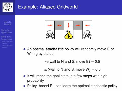
White–Box approach
Use an explorative, stochastic policy and make use ofthe knowledge of your policyWe now compute the gradient analyticallyAssume we know the gradient ∇θπθ(s,a)

MarcelloRestelli
Black–BoxApproaches
White–BoxApproachesMonte–Carlo PolicyGradient
Actor–Critic PolicyGradient
Likelihood Ratio Gradient
For a cost function
J(θ) =
∫T
pθ(τ |π)R(τ)dτ
we have the gradient
∇θJ(θ) = ∇θ∫T
pθ(τ |π)R(τ)dτ =
∫T∇θpθ(τ |π)R(τ)dτ
Using the trick
∇θpθ(τ |π) = pθ(τ |π)∇θ log pθ(τ |π)
We obtain
∇θJ(θ) =
∫T
pθ(τ |π)∇ log pθ(τ |π)R(τ)dτ
= E[∇θ log pθ(τ |π)R(τ)]
≈ 1K
K∑k=1
∇θ log pθ(τk |π)R(τk )
Needs only samples!
MarcelloRestelli
Black–BoxApproaches
White–BoxApproachesMonte–Carlo PolicyGradient
Actor–Critic PolicyGradient
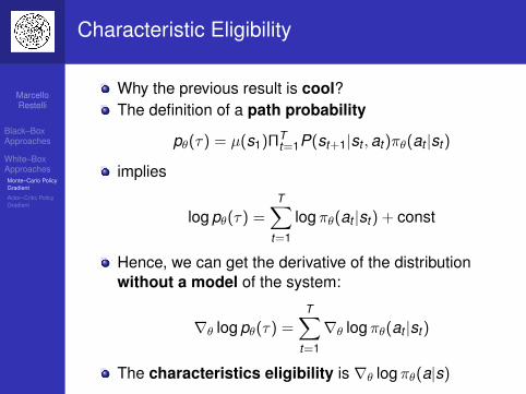
Characteristic Eligibility
Why the previous result is cool?The definition of a path probability
pθ(τ) = µ(s1)ΠTt=1P(st+1|st ,at )πθ(at |st )
implies
log pθ(τ) =T∑
t=1
logπθ(at |st ) + const
Hence, we can get the derivative of the distributionwithout a model of the system:
∇θ log pθ(τ) =T∑
t=1
∇θ logπθ(at |st )
The characteristics eligibility is ∇θ logπθ(a|s)

MarcelloRestelli
Black–BoxApproaches
White–BoxApproachesMonte–Carlo PolicyGradient
Actor–Critic PolicyGradient
Softmax Policy
We will use softmax policy as a running exampleWeight actions using linear combination of featuresφ(s,a)Tθ
Probability of action is proportional to exponentialweight
πθ(s,a) ∝ eφ(s,a)Tθ
The characteristic eligibility is
∇θ logπθ(a|s) = φ(s,a)− Eπθ [φ(s, ·)]
MarcelloRestelli
Black–BoxApproaches
White–BoxApproachesMonte–Carlo PolicyGradient
Actor–Critic PolicyGradient
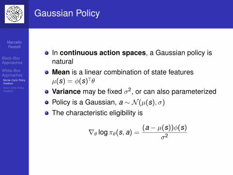
Gaussian Policy
In continuous action spaces, a Gaussian policy isnaturalMean is a linear combination of state featuresµ(s) = φ(s)Tθ
Variance may be fixed σ2, or can also parameterizedPolicy is a Gaussian, a ∼ N (µ(s), σ)
The characteristic eligibility is
∇θ logπθ(s,a) =(a− µ(s))φ(s)
σ2

MarcelloRestelli
Black–BoxApproaches
White–BoxApproachesMonte–Carlo PolicyGradient
Actor–Critic PolicyGradient
One–Step MDPs
Consider a simple class of one–step MDPsStarting in state s ∼ d(·)Terminating after one time–step with rewardr = R(s,a)
Use likelihood ratios to compute policy gradient
J(θ) = Eπθ [r ]
=∑s∈S
d(s)∑a∈A
πθ(a|s)R(s,a)
∇θJ(θ) =∑s∈S
d(s)∑a∈A
πθ(a|s)∇θ logπθ(a|s)R(s,a)
= Eπθ [∇θ logπθ(a|s)r ]

MarcelloRestelli
Black–BoxApproaches
White–BoxApproachesMonte–Carlo PolicyGradient
Actor–Critic PolicyGradient
Policy Gradient Theorem
The policy gradient theorem generalize the likelihoodratio approach to multi–step MDPsReplaces instantaneous reward r with long–termvalue Qπ(s,a)
Policy gradient theorem applies to start state objective,average reward and average value objective
TheoremFor any differentiable policy πθ(a|s), for any of the policyobjective functions J = J1, JavR, or 1
1−γ JavV , the policygradient is
∇θJ(θ) = Eπθ [∇θ logπθ(a|s)Qπθ(s,a)]

MarcelloRestelli
Black–BoxApproaches
White–BoxApproachesMonte–Carlo PolicyGradient
Actor–Critic PolicyGradient
Monte–Carlo Policy Gradient
Update parameters by stochastic gradient ascentUsing policy gradient theoremUsing return vt as an unbiased sample of Qπθ(st ,at )
∆θt = α∇θ logπθ(at |st )vt
function REINFORCE()Initialize θ arbitrarilyfor all episodes {s1,a1, r2, . . . , sT−1,aT−1, rT} ∼ πθ do
for t = 1 to T − 1 doθ ← θ + α∇θ logπθ(at , st )vt
end forend forreturn θ
end function

MarcelloRestelli
Black–BoxApproaches
White–BoxApproachesMonte–Carlo PolicyGradient
Actor–Critic PolicyGradient
Puck World Example
Continuous actions exert small force on puckPuck is rewarded for getting close to targetTarget location is reset every 30 secondsPolicy is trained using variant (conjugate) ofMonte–Carlo policy gradient
MarcelloRestelli
Black–BoxApproaches
White–BoxApproachesMonte–Carlo PolicyGradient
Actor–Critic PolicyGradient
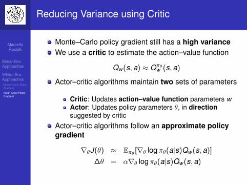
Reducing Variance using Critic
Monte–Carlo policy gradient still has a high varianceWe use a critic to estimate the action–value function
Qw (s,a) ≈ Qπθw (s,a)
Actor–critic algorithms maintain two sets of parameters
Critic: Updates action–value function parameters wActor: Updates policy parameters θ, in directionsuggested by critic
Actor–critic algorithms follow an approximate policygradient
∇θJ(θ) ≈ Eπθ [∇θ logπθ(a|s)Qw (s,a)]
∆θ = α∇θ logπθ(a|s)Qw (s,a)

MarcelloRestelli
Black–BoxApproaches
White–BoxApproachesMonte–Carlo PolicyGradient
Actor–Critic PolicyGradient
Estimating the Action–Value Function
The critic is solving a familiar problem: policyevaluationHow good is policy πθ for current parameters θ?
Monte Carlo policy evaluationTemporal–Difference learningTD(λ)
Could also use e.g., least–squares policy evaluation
MarcelloRestelli
Black–BoxApproaches
White–BoxApproachesMonte–Carlo PolicyGradient
Actor–Critic PolicyGradient
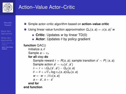
Action–Value Actor–Critic
Simple actor–critic algorithm based on action–value critic
Using linear value function approximation Qw (s, a) = φ(s, a)Tw
Critic: Updates w by linear TD(0)Actor: Updates θ by policy gradient
function QAC()Initialize s, θSample a ∼ πθfor all step do
Sample reward r = R(s, a); sample transition s′ ∼ P(·|s, a)Sample action a′ ∼ πθ(s′, a′)δ = r + γQw (s′, a′)−Qw (s, a)θ = θ + α∇θ logπθ(s, a)Qw (s, a)w ← w + βδφ(s, a)a← a′, s ← s′
end forend function

MarcelloRestelli
Black–BoxApproaches
White–BoxApproachesMonte–Carlo PolicyGradient
Actor–Critic PolicyGradient
Bias in Actor–Critic Algorithms
Approximating the policy gradient introduces biasA biased policy gradient may not find the right solutionLuckily, if we choose action–value functionapproximation carefullyThen we can avoid introducing any biasi.e., We can still follow the exact policy gradient

MarcelloRestelli
Black–BoxApproaches
White–BoxApproachesMonte–Carlo PolicyGradient
Actor–Critic PolicyGradient
Compatible Function Approximation
Theorem (Compatible Function Approximation Theorem)If the following two conditions are satisfied:
1 Value function approximation is compatible to the policy
∇wQw (s,a) = ∇θ logπθ(a|s)
2 Value function parameters w minimize themean–squared error
ε = Eπθ [(Qπθ(s,a)−Qw (s,a))2]
Then the policy gradient is exact
∇θJ(θ) ≈ Eπθ [∇θ logπθ(a|s)Qw (s,a)]

MarcelloRestelli
Black–BoxApproaches
White–BoxApproachesMonte–Carlo PolicyGradient
Actor–Critic PolicyGradient
Proof of Compatible Function ApproximationTheorem
If w is chosen to minimize mean–squared error, gradient of ε w.r.t. wmust be zero:
∇wε = 0
Eπθ [(Qπθ (s, a)−Qw (s, a))∇w Qw (s, a)] = 0
Eπθ [(Qπθ (s, a)−Qw (s, a))∇θ logπθ(a|s)] = 0
Eπθ [Qπθ (s, a)∇θ logπθ(a|s)] = Eπθ [Qw (s, a)∇θ logπθ(a|s)]
So Qw (s, a) can be substituted directly into the policy gradient
∇θJ(θ) = Eπθ [∇θ logπθ(a|s)Qw (s, a)]

MarcelloRestelli
Black–BoxApproaches
White–BoxApproachesMonte–Carlo PolicyGradient
Actor–Critic PolicyGradient
All–Action Gradient
By integrating over all possible actions in a state, thegradient becomes
∇θJ(θ) =
∫S
dπθ (s)∫A∇θπθ(a|s)Qw (s, a)dads
=
∫S
dπθ (s)∫Aπθ(a|s)∇θ logπθ(a|s)∇θ logπθ(a|s)
Twdads
= F (θ)w
It can be shown that the all–action matrix F (θ) isequal to the Fisher information matrix G(θ)
G(θ) =
∫S
dπθ (s)∫Aπθ(a|s)∇θ log (dπθ (s)πθ(a|s))∇θ log (dπθ (s)πθ(a|s))
Tdads
=
∫S
dπθ (s)∫Aπθ(a|s)∇θ logπθ(a|s)∇θ logπθ(a|s)
Tdads
= F (θ)
MarcelloRestelli
Black–BoxApproaches
White–BoxApproachesMonte–Carlo PolicyGradient
Actor–Critic PolicyGradient
Reducing Variance Using a Baseline
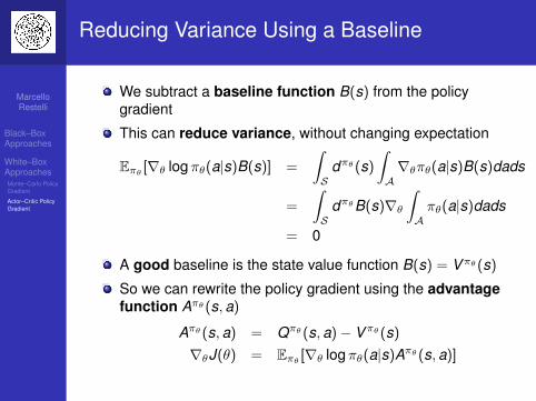
We subtract a baseline function B(s) from the policygradient
This can reduce variance, without changing expectation
Eπθ[∇θ logπθ(a|s)B(s)] =
∫S
dπθ (s)
∫A∇θπθ(a|s)B(s)dads
=
∫S
dπθB(s)∇θ∫Aπθ(a|s)dads
= 0
A good baseline is the state value function B(s) = Vπθ (s)
So we can rewrite the policy gradient using the advantagefunction Aπθ (s,a)
Aπθ (s,a) = Qπθ (s,a)− Vπθ (s)
∇θJ(θ) = Eπθ[∇θ logπθ(a|s)Aπθ (s,a)]

MarcelloRestelli
Black–BoxApproaches
White–BoxApproachesMonte–Carlo PolicyGradient
Actor–Critic PolicyGradient
Estimating the Advantage Function
The compatible function approximator is mean–zero!∫A∇θ logπθ(a|s)wda =
∫A
∇θπθ(a|s)
πθ(a|s)wda = 0
So the critic should really estimate the advantage function
The advantage function can significantly reduce variance of policygradient
Traditional value function learning methods (e.g., TD) cannot beapplied
Using two function approximators and two parameter vectors
Vv (s) ≈ Vπθ (s)
Qw (s, a) ≈ Qπθ (s, a)
A(s, a) = Qw (s, a)− Vv (s)
And updating both value functions by e.g., TD learning

MarcelloRestelli
Black–BoxApproaches
White–BoxApproachesMonte–Carlo PolicyGradient
Actor–Critic PolicyGradient
Estimating the Advantage Function
For the true value function Vπθ (s), the TD–error δπθ
δπθ = r + γVπθ (s′)− Vπθ (s)
is an unbiased estimate of the advantage function
Eπθ [δπθ ] = Eπθ [r + γVπθ (s′)|s, a]− Vπθ (s)
= Qπθ (s, a)− Vπθ (s)
= Aπθ (s, a)
So we can use the TD error to compute the policy gradient
∇θJ(θ) = Eπθ [∇θ logπθ(a|s)δπθ ]
In practice we can use an approximate TD error
δv = r + γVv (s′)− Vv (s)
This approach only requires one set of critic parameters v

MarcelloRestelli
Black–BoxApproaches
White–BoxApproachesMonte–Carlo PolicyGradient
Actor–Critic PolicyGradient
Actors at Different Time–Scales
As the critic, also the actor can estimate policy gradientat many time–scales
∇θJ(θ) = Eπθ [∇θ logπθ(a|s)Aπθ(s,a)]
Monte–Carlo policy gradient uses error from completereturn
∆θ = α(vt − Vv (st ))∇θ logπθ(at |st )
Actor–critic policy gradient uses one–step TD error
∆θ = α(r + γVv (st+1)− Vv (st ))∇θ logπθ(at |st )

MarcelloRestelli
Black–BoxApproaches
White–BoxApproachesMonte–Carlo PolicyGradient
Actor–Critic PolicyGradient
Policy Gradient with Eligibility Traces
Just like forward–view TD(λ), we can mix overtime–scales
∆θ = α(vλt − Vv (st ))∇θ logπθ(at |st )
where vλt − Vv (st ) is a biased estimate of advantagefunctionLike backward–view TD(λ), we can also use eligibilitytracesBy equivalence with TD(λ), substitutingφ(s) = ∇θ logπθ(a|s)
δ = rt+1 + γVv (st+1)− Vv (st )
et+1 = λet +∇θ logπθ(a|s)
∆θ = αδet
This update can be applied online, to incompletesequences

MarcelloRestelli
Black–BoxApproaches
White–BoxApproachesMonte–Carlo PolicyGradient
Actor–Critic PolicyGradient
Alternative Policy Gradient Directions
Gradient ascent algorithms can follow any ascentdirectionA good ascent direction can significantly speedconvergenceAlso, a policy can often be re–parameterized withoutchanging action probabilitiesFor example, increasing score of all actions in asoftmax policyThe vanilla gradient is sensitive to thesere–parameterization

MarcelloRestelli
Black–BoxApproaches
White–BoxApproachesMonte–Carlo PolicyGradient
Actor–Critic PolicyGradient
Natural Policy Gradient
A more efficient gradient in learning problems is the natural gradientIt finds ascent direction that is closest to vanilla gradient, when changingpolicy by a small, fixed amount
∇̃θJ(θ) = G−1(θ)∇θJ(θ)
Where G(θ) is the Fisher information matrix
G(θ) = Eπθ [∇θ logπθ(a|s)∇θ logπθ(a|s)T]
Natural policy gradients are independent of the chosen policyparameterizationThey correspond to steepest ascent in policy space and not in theparameter spaceConvergence to a local minimum is guaranteed
MarcelloRestelli
Black–BoxApproaches
White–BoxApproachesMonte–Carlo PolicyGradient
Actor–Critic PolicyGradient
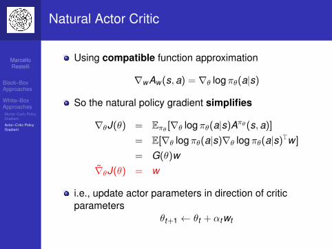
Natural Actor Critic
Using compatible function approximation
∇wAw (s,a) = ∇θ logπθ(a|s)
So the natural policy gradient simplifies
∇θJ(θ) = Eπθ [∇θ logπθ(a|s)Aπθ(s,a)]
= E[∇θ logπθ(a|s)∇θ logπθ(a|s)Tw ]
= G(θ)w∇̃θJ(θ) = w
i.e., update actor parameters in direction of criticparameters
θt+1 ← θt + αtwt

MarcelloRestelli
Black–BoxApproaches
White–BoxApproachesMonte–Carlo PolicyGradient
Actor–Critic PolicyGradient
Episodic Natural Actor Critic
Critic: Episodic EvaluationSufficient Statistics
Φ =
[φ1 φ2 . . . φN1 1 . . . 1
]TR =
[R1 R2 . . . RN
]TLinear Regression[
wJ
]= (ΦTΦ)−1ΦTR
Actor: Natural Policy Gradient Improvement
θt+1 = θt + αtwt

MarcelloRestelli
Black–BoxApproaches
White–BoxApproachesMonte–Carlo PolicyGradient
Actor–Critic PolicyGradient
Learning Ball in a Cup
Ball in a cup
Related Documents