Regression Models for Time Series Analysisbnk/Ch_GLMsld.pdf · Regression Models for Time Series Analysis Benjamin Kedem1 and Konstantinos Fokianos2 1University of Maryland, College

Regression Models for Time SeriesAnalysis

Benjamin Kedem1

and

Konstantinos Fokianos2

1University of Maryland, College Park, MD2University of Cyprus, Nicosia, Cyprus

Wiley, New York, 2002

1

Cox (1975). Partial likelihood, Biometrika, 62,

69–76.

Fahrmeir and Tutz (2001). Multivariate Sta-

tistical Modelling Based on GLM. 2nd ed., Springer,

NY.

Fokianos (1996). Categorical Time Series: Pre-

diction and Control. Ph.D. Thesis, University

of Maryland.

Fokianos and Kedem (1998), Prediction and

classification of non-stationary categorical time

series. J. Multivariate Analysis,67, 277-296.

Kedem (1980). Binary Time Series, Marcel

Dekker, NY

(•) Kedem and Fokianos (2002). Regression

Models for Time Series Analysis, Wiley, NY.

2

McCullagh and Nelder (1989). Generalized Lin-

ear Models. 2nd edi., Chapman & Hall, Lon-

don.

Nelder and Wedderburn (1972). Generalized

linear models. JRSS, A, 135, 370–384.

Slud (1982). Consistency and efficiency of in-

ference with the partial likelihood. Biometrika,

69, 547–552.

Slud and Kedem (1994). Partial likelihood

analysis of logistic regression and autoregres-

sion. Statistica Sinica, 4, 89–106.

Wong (1986). Theory of partial likelihood.

Annals of Statistics, 14, 88–123.

3

Part I: GLM and Time Series

Overview

Extension of Nelder and Wedderburn (1972),

McCullagh and Nelder(1989) GLM to time se-

ries is possible due to:

• Increasing sequence of histories relative to

an observer.

• Partial likelihood.

• The partial score is a martingale.

• Well behaved covariates.

4

Partial Likelihood

Suppose we observe a pair of jointly distributed

time series, (Xt, Yt), t = 1, . . . , N , where {Yt} is

a response series and {Xt} is a time dependent

random covariate. Employing the rules of con-

ditional probability, the joint density of all the

X, Y observations can be expressed as,

fθ(x1, y1, . . . , xN , yN) =

fθ(x1)

N∏

t=2

fθ(xt | dt)

N∏

t=1

fθ(yt | ct)

(1)

dt = (y1, x1, . . . , yt−1, xt−1)

ct = (y1, x1, . . . , yt−1, xt−1, xt).

The second product on the right hand side of

(1) constitutes a partial likelihood according to

Cox(1975).

5

An increasing sequence of σ-fields

F0 ⊂ F1 ⊂ F2 . . ..

Y1, Y2, . . . a sequence of random variables on

some common probability space such that Yt

is Ft measurable.

Yt | Ft−1 ∼ ft(yt; θ).

θ ∈ Rp is a fixed parameter.

The partial likelihood (PL) function relative to

θ, Ft, and the data Y1, Y2, . . . , YN , is given by

the product

PL(θ; y1, . . . , yN) =N∏

t=1

ft(yt; θ) (2)

6

The General Regression Problem

{Yt} is a response time series with the corre-

sponding p–dimensional covariate process,

Zt−1 = (Z(t−1)1, . . . , Z(t−1)p)′.

Define,

Ft−1 = σ{Yt−1, Yt−2, . . . ,Zt−1,Zt−2, . . .}.Note: Zt−1 may already include past Yt’s.

The conditional expectation of the response

given the past:

µt = E[Yt | Ft−1],

(•) The problem is to relate µt to the covari-

ates.

7

Time Series Following GLM

1. Random Component. The conditional

distribution of the response given the past be-

longs to the exponential family of distributions

in natural or canonical form,

f(yt; θt, φ | Ft−1) = exp

{

ytθt − b(θt)

αt(φ)+ c(yt;φ)

}

.

(3)

αt(φ) = φ/ωt, dispersion φ, prior weight ωt.

2. Systematic Component. There is a mono-

tone function g(·) such that,

g(µt) = ηt =p∑

j=1

βjZ(t−1)j = Z′t−1β. (4)

g(·): the link function

ηt: the linear predictor of the model.

8

Typical choices for ηt = Z′t−1β, could be

β0 + β1Yt−1 + β2Yt−2 + β3Xt cos(ω0t)

or

β0 + β1Yt−1 + β2Yt−2 + β3Yt−1Xt + β4Xt−1

or

β0 + β1Yt−1 + β2Y 7t−2 + β3Yt−1 log(Xt−12)

9

GLM Equations:∫

f(y; θt;φ | Ft−1)dy = 1.

This implies the relationships:

µt = E[Yt | Ft−1] = b′(θt). (5)

Var[Yt | Ft−1] = αt(φ)b′′(θt) ≡ αt(φ)V (µt). (6)

Since Var[Yt | Ft−1] > 0, it follows that b′ is

monotone. Therefore, equation (5) implies

that

θt = (b′)−1(µt). (7)

We see that θt itself is a monotone function

of µt and hence it can be used to define a link

function. The link function

g(µt) = θt(µt) = ηt = Z′t−1β (8)

is called the canonical link function.

10

Example: Poisson Time Series.

f(yt; θt, φ | Ft−1) = exp {(yt logµt − µt) − log yt!} .

E[Yt|Ft−1] = µt, b(θt) = µt = exp(θt), V (µt) =

µt, φ = 1, and ωt = 1. The canonical link is

g(µt) = θt(µt) = logµt = ηt = Z′t−1β.

As an example , if Zt−1 = (1, Xt, Yt−1)′, then

logµt = β0 + β1Xt + β2Yt−1

with {Xt} standing for some covariate process,

or a possible trend, or a possible seasonal com-

ponent.

11

Example: Binary Time Series

{Yt} takes the values 0,1. Let

πt = P(Yt = 1 | Ft−1).

Then

f(yt; θt, φ | Ft−1) =

exp

{

yt log

(

πt

1 − πt

)

+ log(1 − πt)

}

The canonical link gives the logistic regression

model

g(πt) = θt(πt) = logπt

1 − πt= ηt = Z′

t−1β. (9)

Note:

πt = Fl(ηt) (10)

12

Partial Likelihood Inference

Given a time series {Yt}, t = 1, . . . , N , con-

ditionally distributed as (3).

The partial likelihood of the observed series

is

PL(β) =N∏

t=1

f(yt; θt, φ | Ft−1). (11)

Then from (3), the log–partial likelihood, l(β),

is given by

l(β) =N∑

t=1

log f(yt; θt, φ | Ft−1) ≡N∑

t=1

lt

=N∑

t=1

{

ytθt − b(θt)

αt(φ)+ c(yt, φ)

}

=N∑

t=1

{

ytu(z′t−1β) − b(u(z′t−1β))

αt(φ)+ c(yt, φ)

}

(12)

13

∇ ≡(

∂

∂β1,

∂

∂β2, · · · , ∂

∂βp

)′.

The partial score is a p–dimensional vector,

SN(β) ≡ ∇l(β) =N∑

t=1

Zt−1∂µt

∂ηt

(Yt − µt(β))

σ2t (β)

(13)

with σ2t (β) = Var[Yt | Ft−1].

The partial score vector process {St(β)}, t =

1, . . . , N , is defined from the partial sums

St(β) =t∑

s=1

Zs−1∂µs

∂ηs

(Ys − µs(β))

σ2s (β)

. (14)

14

The solution of the score equation,

SN(β) = ∇ logPL(β) = 0 (15)

is denoted by β̂, and is referred to as the max-

imum partial likelihood estimator (MPLE) of

β. The system of equations (15) is non–linear

and is customarily solved by the Fisher scoring

method, an iterative algorithm resembling the

Newton–Raphson procedure. Before turning

to the Fisher scoring algorithm in our context

of conditional inference, it is necessary to in-

troduce several important matrices.

15

An important role in partial likelihood inference

is played by the cumulative conditional infor-

mation matrix, GN(β), defined by a sum of

conditional covariance matrices,

GN(β) =N∑

t=1

Cov

[

Zt−1∂µt

∂ηt

(Yt − µt(β))

σ2t (β)

| Ft−1

]

=N∑

t=1

Zt−1

(

∂µt

∂ηt

)21

σ2t (β)

Z′t−1

= Z′W(β)Z.

We also need:

HN(β) ≡ −∇∇ ′l(β).

Define RN(β) from the difference

HN(β) = GN(β) − RN(β).

Fact: For canonical links RN(β) = 0.

16

Fisher Scoring: In Newton-Raphson replace

HN(β) by its conditional expectation:

β̂(k+1)

= β̂(k)

+ G−1N (β̂

(k))SN(β̂

(k)).

Fisher scoring becomes Newton-Raphson for

canonical links.

Fisher scoring simplifies to Iterative Reweighted

Least Squares:

β̂(k+1)

=

(

Z′W(β̂(k)

)Z

)−1Z′W(β̂

(k))q(k).

17

Asymptotic Theory

Assumption A

A1. The true parameter β belongs to an open

set B ⊆ Rp.

A2. The covariate vector Zt−1 almost surely

lies in a nonrandom compact subset Γ of Rp,

such that P [∑N

t=1 Zt−1Z′t−1 > 0] = 1. In ad-

dition, Z′t−1β lies almost surely in the domain

H of the inverse link function h = g−1 for all

Zt−1 ∈ Γ and β ∈ B.

A3. The inverse link function h–defined in

(A2)–is twice continuously differentiable and

|∂h(γ)/∂γ| 6= 0.

18

A4. There is a probability measure ν on Rp

such that∫

Rp zz′ν(dz) is positive definite, and

such that under (3) and (4) for Borel sets

A ⊂ Rp,

1

N

N∑

t=1

I[Zt−1∈A]→ν(A)

in probability as N → ∞, at the true value of β.

A4 calls for asymptotically “well behaved” co-

variates:∑N

t=1 f(Zt−1)

N→∫

Rpf(z)ν(dz)

in probability as N → ∞. Thus, there exists a

p × p limiting information matrix per observa-

tion, G(β), such that

GN(β)

N→ G(β) (16)

in probability, as N → ∞.

19

Slud and K (1994), Fokianos and K (1998):

1. {St(β)} relative to {Ft}, t = 1, . . . , N , is

a martingale.

2.RN(β)

N → 0.

3.SN(β)√

N→ Np(0, G(β)).

4.√

N(β̂ − β)→Np(0,G−1(β)).

20

100(1 − α)% prediction interval (h = g−1)

µt(β)·= µt(β̂)±zα/2

|h′(Z′t−1β)|√N

√

Z′t−1G

−1(β)Zt−1

Hypothesis Testing

Let β̃ be the MPLE of β obtained under H0

with r < p restrictions,

H0 : β1 = · · · = βr = 0.

Let β̂ be the unrestricted MPLE. The log–

partial likelihood ratio statistic

λN = 2{

l(β̂) − l(β̃)}

(17)

converges to χ2r .

21

More generally:

Assume C is a known matrix with full rank

r, r < p.

Under the general linear hypothesis,

H0 : Cβ = β0 against H1 : Cβ 6= β0, (18)

{Cβ̂ − β0}′{CG−1(β̂)C′}−1{Cβ̂ − β0} → χ2r

22

Diagnostics

l(y;y): maximum log partial likelihood corre-

sponding to the saturated model.

l(µ̂;y): maximum log partial likelihood from

the reduced model.

• Scaled Deviance:

D ≡ 2{l(y;y) − l(µ̂;y)} ∼ χ2N−p

• AIC(p) = −2 logPL(β̂) + 2p,

• BIC(p) = −2 logPL(β̂) + p logN

23

Analysis of Mortality Count Data in LA

Weekly data from Los Angeles County during

a period of 10 years from January 1, 1970, to

December 31, 1979: Weekly sampled filtered

time series. N = 508.

Response

Y Total Mortality (filtered)

WeatherT TemperatureRH Relative humidity

PollutionCO Carbon monoxideSO2 Sulfur dioxideNO2 Nitrogen dioxideHC HydrocarbonsOZ OzoneKM Particulates

24

0 100 200 300 400 500

140

160

180

200

220

Mortality

Lag

AC

F

0 5 10 15 20 25

0.0

0.2

0.4

0.6

0.8

1.0

Series : Mort

0 100 200 300 400 500

5060

7080

9010

0

Temperature

Lag

AC

F

0 5 10 15 20 25

-0.5

0.0

0.5

1.0

Series : Temp

0 100 200 300 400 500

1.0

1.5

2.0

2.5

3.0

log(CO)

Lag

AC

F

0 5 10 15 20 25

-0.4

0.0

0.2

0.4

0.6

0.8

1.0

Series : log(CO)

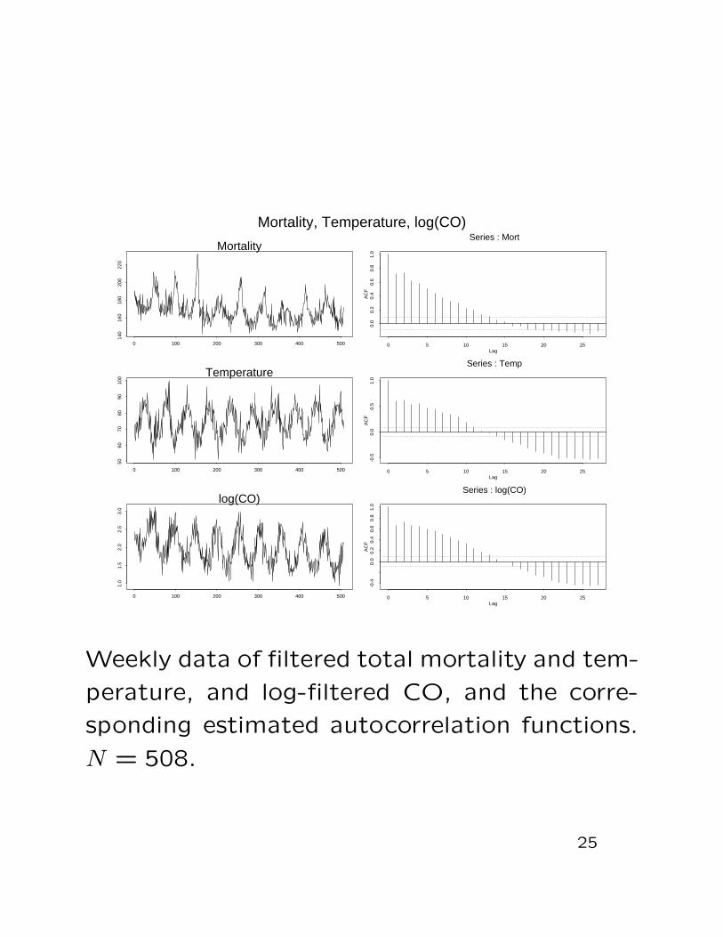
Mortality, Temperature, log(CO)

Weekly data of filtered total mortality and tem-

perature, and log-filtered CO, and the corre-

sponding estimated autocorrelation functions.

N = 508.

25

Covariates and ηt used in Poisson regression.

S = SO2, N = NO2. To recover ηt, insert the

β’s. For Model 2, ηt = β0 + β1Yt−1 + β2Yt−2,

etc.

Model 0 Tt + RHt + COt + St + Nt+HCt + OZt + KMt

Model 1 Yt−1Model 2 Yt−1 + Yt−2Model 3 Yt−1 + Yt−2 + Tt−1Model 4 Yt−1 + Yt−2 + Tt−1 + log(COt)Model 5 Yt−1 + Yt−2 + Tt−1 + Tt−2 + log(COt)Model 6 Yt−1 + Yt−2 + Tt + Tt−1 + log(COt)

26

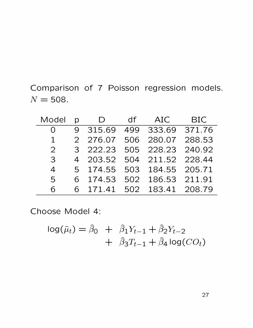
Comparison of 7 Poisson regression models.

N = 508.

Model p D df AIC BIC

0 9 315.69 499 333.69 371.761 2 276.07 506 280.07 288.532 3 222.23 505 228.23 240.923 4 203.52 504 211.52 228.444 5 174.55 503 184.55 205.715 6 174.53 502 186.53 211.916 6 171.41 502 183.41 208.79

Choose Model 4:

log(µ̂t) = β̂0 + β̂1Yt−1 + β̂2Yt−2

+ β̂3Tt−1 + β̂4 log(COt)

27

0 100 200 300 400 500

140

160

180

200

220

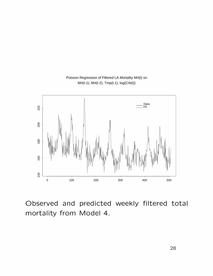
____ Data........ Fit

Poisson Regression of Filtered LA Mortality Mrt(t) on

Mrt(t-1), Mrt(t-2), Tmp(t-1), log(Crb(t))

Observed and predicted weekly filtered total

mortality from Model 4.

28

Model 0 Residuals

0 100 200 300 400 500

-0.1

0.1

0.3

Model 4 Residuals

0 100 200 300 400 500

-0.1

50.

00.

10

Lag

AC

F

0 5 10 15 20 25

0.0

0.4

0.8

Series : Resid0

Lag

AC

F

0 5 10 15 20 25

0.0

0.4

0.8

Series : Resid4

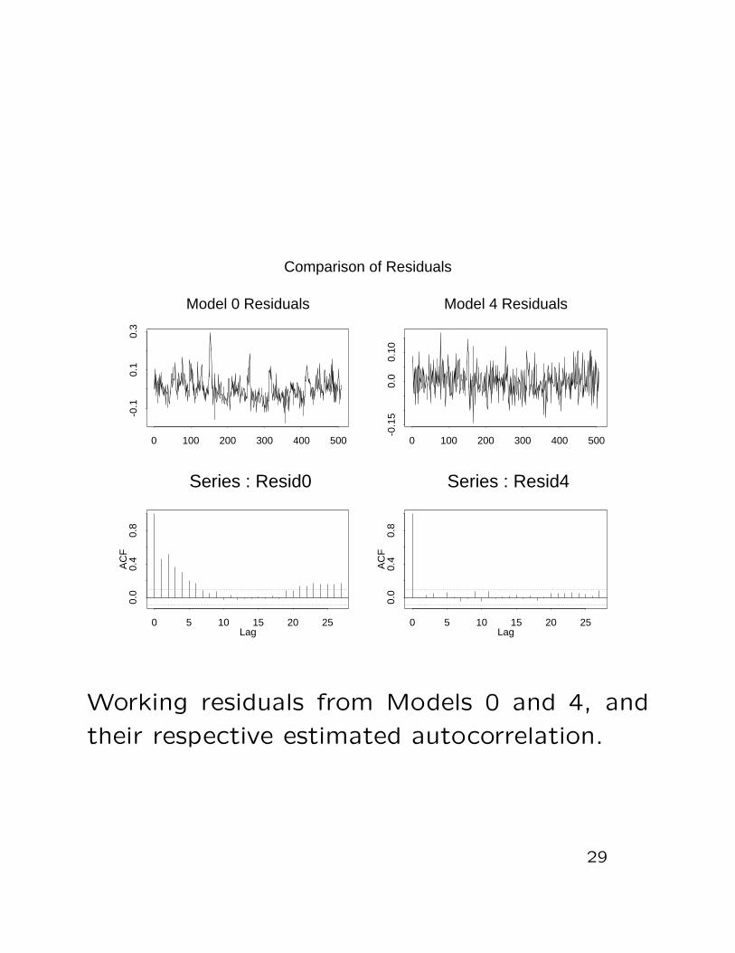
Comparison of Residuals

Working residuals from Models 0 and 4, and

their respective estimated autocorrelation.

29

Part II: Binary Time Series

Example of bts: Two categories obtained by

clipping.

Yt ≡ I[Xt∈C] =

{

1, if Xt ∈ C0, if Xt ∈ C

(19)

Yt ≡ I[Xt≥r] =

{

1, if Xt ≥ r0, if Xt < r

(20)

Other examples: at time t = 1,2, .....,

(Rain, No Rain), (S&P Up, S&P Down), etc.

30

{Yt} taking the values 0 or 1, t = 1,2,3, · · ·.

{Zt−1} p-dim covariate stochastic data.

Against the backdrop of the general framework

presented above we wish to relate

µt(β) = πt(β) = Pβ(Yt = 1|Ft−1) (21)

to the covariates. For this we need good links!

31

Standard logistic distribution,

Fl(x) =ex

1 + ex=

1

1 + e−x, −∞ < x < ∞

Then,

F−1l (x) = log(x/(1 − x))

is the natural link under some conditions.

32

• Fact: For any bts, there are θj such that

log

{

P(Yt = 1|Yt−1 = yt−1, ..., Y1 = y1)

P(Yt = 0|Yt−1 = yt−1, ..., Y1 = y1)

}

=

θ0 + θ1yt−1 + · · · + θpyt−p

or

πt(β) =1

1 + exp[−(θ0 + θ1yt−1 + · · · + θpyt−p)]

• Fact: Consider an AR(p) time series

Xt = γ0 + γ1Xt−1 + . . . + γpXt−p + λǫt

where ǫt are i.i.d. logistically distributed. De-

fine: Yt = I[Xt≥r]. Then

πt(β) =1

1 + exp[−(γ0 − r + γ1Xt−1 + · · · + γpXt−p)/λ]

33

This motivates logistic regression:

πt(β) ≡ Pβ(Yt = 1|Ft−1) = Fl(β′Zt−1)

=1

1 + exp[−β′Zt−1]

or equivalently, the link function is

logit(πt(β)) ≡ log

{

πt(β)

1 − πt(β)

}

= β′Zt−1

This is the canonical link.

34

Link functions for binary time series.

logit β′Zt−1 = log{πt(β)/(1 − πt(β))}probit β′Zt−1 = Φ−1{πt(β)}log-log β′Zt−1 = − log{− log(πt(β))}C-log-log β′Zt−1 = log{− log(1 − πt(β))}

Note: Here all the inverse links are cdf’s. In

what follows we always assume the inverse link

is a differentiable cdf F(x).

35

The partial likelihood of β takes on the simple

product form,

PL(β) =N∏

t=1

[πt(β)]yt[1 − πt(β)]1−yt

=N∏

t=1

[F(β′Zt−1)]yt[1 − F(β′Zt−1)]

1−yt

We have under Assumption A:

√N(β̂ − β)→Np(0,G−1(β)).

For the canonical link (logistic regression):

GN(β)

N→ G(β) =

∫

Rp

eβ′z

(1 + eβ′z)2

zz′ν(dz)

36

Illustration of asymptotic normality.

logit(πt(β)) = β1 + β2 cos

(

2πt

12

)

+ β3Yt−1

so that Zt−1 = (1, cos(2πt/12), Yt−1)′.

(a)

0 50 100 150 200

0.0

0.4

0.8

(b)

t0 50 100 150 200

0.4

0.6

0.8

Logistic autoregression with a sinusoidal com-ponent. a. Yt. b. πt(β) where logit(πt(β)) =0.3 + 0.75 cos(2πt/12) + yt−1.

37

-2 -1 0 1 2 3 4

0.0

0.1

0.2

0.3

0.4

b1

-2 0 2 4

0.0

0.1

0.2

0.3

0.4

b2

-4 -2 0 2

0.0

0.1

0.2

0.3

0.4

b3

Histograms of normalized MPLE’s where β =

(0.3,0.75,1)′, N = 200. Each histogram con-

sists of 1000 estimates.

38

Goodness of Fit

C1, · · · , Ck, a partition of Rp. For j = 1, · · · , k,define,

Mj ≡N∑

t=1

I[Zt−1∈Cj]Yt

and

Ej(β) ≡N∑

t=1

I[Zt−1∈Cj]πt(β)

Put:

M ≡ (M1, · · · , Mk)′,

E(β) ≡ (E1(β), · · · , Ek(β))′.

39

Slud and K (1994), K and Fokianos (2002):

With

σ2j ≡

∫

Cj

F(β′z)(1 − F(β′z))ν(dz)

χ2(β) ≡ 1

N

k∑

j=1

(Mj − Ej(β))2/σ2j → χ2

k.

In practice need to adjust the df when replacing

β by β̂.

40

When β̂ and (M−E(β)) are obtained from the

same data set,

E(χ2(β̂)) ≈ k −k∑

j=1

(B′G(β)B)jj/σ2j

When β̂ and (M − E(β)) are obtained from

independent data sets,

E(χ2(β̂)) ≈ k +k∑

j=1

(B′G(β)B)jj/σ2j

41

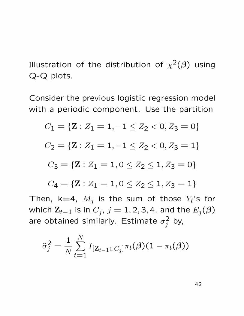
Illustration of the distribution of χ2(β) using

Q-Q plots.

Consider the previous logistic regression model

with a periodic component. Use the partition

C1 = {Z : Z1 = 1,−1 ≤ Z2 < 0, Z3 = 0}

C2 = {Z : Z1 = 1,−1 ≤ Z2 < 0, Z3 = 1}

C3 = {Z : Z1 = 1,0 ≤ Z2 ≤ 1, Z3 = 0}

C4 = {Z : Z1 = 1,0 ≤ Z2 ≤ 1, Z3 = 1}Then, k=4, Mj is the sum of those Yt’s for

which Zt−1 is in Cj, j = 1,2,3,4, and the Ej(β)

are obtained similarly. Estimate σ2j by,

σ̃2j =

1

N

N∑

t=1

I[Zt−1∈Cj]πt(β)(1 − πt(β))

42

The χ24 approximation is quite good.

•••••••••••••••••••••••••••••••••••••••••••••••••••••••••••••••••••••••••••••••••••••••••••••••••••••••••••••••••••••••••••••••••••••••••••••••••••••••••••••••••••••••••••••••••••••••••••••••••••••••••••••••••••••••••••••••••••••••••••••••••••••••••••••••••••••••••••••••••••••••••••••••••••••••••••••••••••••••••••••••••••••••••••••••••••••••••••••••••••••••••••••••••••••••••••••••••••••••••••••••••••••••••••••••••••••••••••••••••••••••••••••••••••••••••••••••••••••••••••••••••••••••••••••••••••••••••••••••••••••••••••••••••••••••••••••••••••••••••••••••••••••••••••••••••••••••••••••••••••••••••••••••••••••••••••••••••••••••••••••••••••••••••••••••••••••••••••••••••••••••••••••••••••••••••••••••••••••••••••••••

•••••••••••••••••••••

•• •

CHI SQ STATISTIC

TR

UE

CH

I SQ

0 5 10 15 20 25

02

46

810

1214

N=200, b=(0.3,0.75,1)

•••••••••••••••••••••••••••••••••••••••••••••••••••••••••••••••••••••••••••••••••••••••••••••••••••••••••••••••••••••••••••••••••••••••••••••••••••••••••••••••••••••••••••••••••••••••••••••••••••••••••••••••••••••••••••••••••••••••••••••••••••••••••••••••••••••••••••••••••••••••••••••••••••••••••••••••••••••••••••••••••••••••••••••••••••••••••••••••••••••••••••••••••••••••••••••••••••••••••••••••••••••••••••••••••••••••••••••••••••••••••••••••••••••••••••••••••••••••••••••••••••••••••••••••••••••••••••••••••••••••••••••••••••••••••••••••••••••••••••••••••••••••••••••••••••••••••••••••••••••••••••••••••••••••••••••••••••••••••••••••••••••••••••••••••••••••••••••••••••••••••••••••••••••••••••••••••••••

• •

•

CHI SQ STATISTIC

TR

UE

CH

I SQ

0 5 10 15 20

05

1015

N=400, b=(0.3,1,2)

43

Example: Modeling successive eruptions of the

Old Faithful geyser in Yellowstone National Park,

Wyoming.

1 if duration is greater than 3 minutes

0 if duration is less than 3 minutes

10111011010101101011010101011111010101010101010101010101111101010101101011101111101110101010101010101010101010110101010101110111111101111101111111010101010101111110101010111010101101011110101010111010101101101110101010110111111101010111101101110110101110101111101110101011010111111110101010101010110

N = 299

44

Candidate models ηt = β′Zt−1 for Old Faithful.

1 β0 + β1Yt−1

2 β0 + β1Yt−1 + β2Yt−2

3 β0 + β1Yt−1 + β2Yt−2 + β3Yt−3

4 β0 + β1Yt−1 + β2Yt−2 + β3Yt−3 + β4Yt−4

Comparison of models using the logistic link:

Model 2 is “best”. Probit reg. gives similar

results.

Model p X2 D AIC BIC

1 2 165.00 227.38 231.38 238.462 3 165.00 215.53 221.53 232.153 4 165.00 215.08 223.08 237.244 5 164.97 213.99 223.99 241.69

π̂t = πt(β̂) =1

1 + exp{

−(β̂0 + β̂1Yt−1 + β̂2Yt−2)}.

45

Part III: Categorical Time Series

EEG sleep state classified or quantized in four

categories as follows.

1 : quiet sleep,2 : indeterminate sleep,3 : active sleep,4 : awake.

Here the sleep state categories or levels are as-

signed integer values. This is an example of a

categorical time series {Yt}, t = 1, ..., N , taking

the values 1, ...,4.

This is an arbitrary integer assignment. Why

not the values 7.1, 15.8, 19.24, 71.17 ? Any

other scale ?

46

Assume m categories.

The t’th observation of any categorical time

series–regardless of the measurement scale–

can be represented by the vector

Yt = (Yt1, . . . , Ytq)′

of length q = m − 1, with elements

Ytj =

{

1, if the jth category is observed at time t

0, otherwise

for t = 1, . . . , N and j = 1, . . . , q.

BTS is a special case with m = 2, q = 1.

47

Write for j = 1, . . . , q,

πtj = E[Ytj | Ft−1] = P(Ytj = 1 | Ft−1),

Define:

πt = (πt1, . . . πtq)′

Ytm = 1 −q∑

j=1

Ytj

πtm = 1 −q∑

j=1

πtj.

Let {Zt−1}, t = 1, . . . , N , for a p×q matrix that

represents a covariate process.

Ytj corresponds to a vector of length p of ran-

dom time dependent covariates which forms

the jth column of Zt−1.

48

Assume the general regression model:

(∗) πt(β) =

πt1(β)

πt2(β)

· · ·πtq(β)

=

h1(Z′t−1β)

h2(Z′t−1β)

· · ·hq(Z′

t−1β)

= h(Z′t−1β).

The inverse link function h is defined on Rq

and takes values in Rq.

We shall only examine nominal and ordinal time

series.

49

Nominal Time Series.

Nominal categorical variables lack natural or-

dering.

A model for nominal time series: Multinomial

logit model

πtj(β) =exp(β′

jzt−1)

1 +∑q

l=1 exp(β′lzt−1)

, j = 1, . . . , q

Note that

πtm(β) =1

1 +∑q

l=1 exp(β′lzt−1)

.

50

Multinomial logit model is a special case of (*).

Indeed, define β to be the p ≡ qd-vector

β = (β′1, . . . , β′

q)′,

and Zt−1 the qd × q matrix

Zt−1 =

zt−1 0 · · · 0

0 zt−1 · · · 0... ... . . . ...0 0 · · · zt−1

.

Let h stand for the vector valued function whose

components hj, j = 1, . . . , q, are given by

πtj(β) = hj(ηt) =exp(ηtj)

1 +∑q

l=1 exp(ηtl), j = 1, . . . , q

with

ηt = (ηt1, . . . , ηtq)′ = Z′

t−1β.

51

Ordinal Time Series.

Measured on a scale endowed with a natural

ordering.

A model for ordinal time series: Need a la-

tent or auxiliary variable.

Put

Xt = −γ′zt−1 + et,

1. et ∼ cdf F i.i.d.

2. γ d-dim vector of parameters.

3. zt−1 covariate d-dim vector.

Define a categorical time series {Yt}, from the

levels of {Xt},

Yt = j ⇐⇒ Ytj = 1 ⇐⇒ θj−1 ≤ Xt < θj

−∞ = θ0 < θ1 < . . . < θm = ∞.

52

Then

πtj = P(θj−1 ≤ Xt < θj | Ft−1)

= F(θj + γ′zt−1) − F(θj−1 + γ′zt−1),

for j = 1, . . . , m.

There are many possibilities depending on F .

Special case: Proportional Odds Model,

F(x) = Fl(x) =1

1 + exp(−x).

Then we have for j = 1, . . . , q,

log

{

P[Yt ≤ j|Ft−1]

P[Yt > j|Ft−1

}

= θj + γ′zt−1

53

Proportional odds model has the form (*) with

p = (q + d):

β = (θ1, . . . , θq, γ′)′

and Zt−1 the (q + d) × q matrix

Zt−1 =

1 0 · · · 00 1 · · · 0... ... . . . ...0 0 · · · 1

zt−1 zt−1 · · · zt−1

.

Now set

h = (h1, . . . , hq)′,

and let for j = 2, . . . , q,

πt1(β) = h1(ηt) = F(ηt1),

πtj(β) = hj(ηt) = F(ηtj) − F(ηt(j−1)),

where

ηt = (ηt1, . . . , ηtq)′ = Z′

t−1β.

54

Partial likelihood estimation.

Introduce the multinomial probability

f(yt;β | Ft−1) =m∏

j=1

πtj(β)ytj .

The partial likelihood is a product of the multi-

nomial probabilities,

PL(β) =N∏

t=1

f(yt;β|Ft−1)

=N∏

t=1

m∏

j=1

πytjtj (β),

so that the partial log-likelihood is given by

l(β) ≡ logPL(β) =N∑

t=1

m∑

j=1

ytj logπtj(β).

55

Under a modified Assumption A:

GN(β)

N→∫

Rp×qZU(β)Σ(β)U′(β)Z′ν(dZ) = G(β)

√N(β̂ − β)→Np

(

0,G−1(β))

√N(

πt(β̂) − πt(β))

→Nq

(

0,Zt−1Dt(β)G−1(β)D′t(β)Z′

t−1

)

56

Example: Sleep State.

Covariates: Heart Rate, Temperature.

N = 700.

1 : quiet sleep,2 : indeterminate sleep,3 : active sleep,4 : awake.

Ordinal CTS: ”4” < ”1” < ”2” < ”3”.

time

Sta

te

0 200 400 600 800 1000

1.0

2.0

3.0

4.0

time

Hea

rt R

ate

0 200 400 600 800 1000

100

140

180

time

Tem

pera

ture

0 200 400 600 800 1000

36.9

37.2

57

Fit proportional odds models.

Model Covariates AIC

1 1+Yt−1 401.562 1+Yt−1+logRt 401.513 1+Yt−1+logRt+Tt 403.324 1+Yt−1+Tt 403.525 1+Yt−1+Yt−2+logRt 407.286 1+Yt−1+logRt−1 403.407 1+logRt 1692.31

58

Model 2: 1 + Yt−1 + logRt

log

[

P(Yt ≤ ”4” | Ft−1)

P(Yt > ”4” | Ft−1)

]

=

θ1 + γ1Y(t−1)1 + γ2Y(t−1)2 + γ3Y(t−1)3 + γ4 logRt,

log

[

P(Yt ≤ ”1” | Ft−1)

P(Yt > ”1” | Ft−1)

]

=

θ2 + γ1Y(t−1)1 + γ2Y(t−1)2 + γ3Y(t−1)3 + γ4 logRt,

log

[

P(Yt ≤ ”2” | Ft−1)

P(Yt > ”2” | Ft−1)

]

=

θ3 + γ1Y(t−1)1 + γ2Y(t−1)2 + γ3Y(t−1)3 + γ4 logRt,

θ̂1 = −30.352, θ̂2 = −23.493, θ̂3 = −20.349,

γ̂1 = 16.718, γ̂2 = 9.533, γ̂3 = 4.755, γ̂4 =

3.556.

The corresponding standard errors are 12.051,

12.012, 11.985, 0.872, 0.630, 0.501 and 2.470.

59

Sta

te

0 50 100 150 200 250 300

1.0

2.0

3.0

4.0

(a)

Sta

te

0 50 100 150 200 250 300

1.0

2.0

3.0

4.0

(b)

(a) Observed versus (b) predicted sleep states

for Model 2 of Table applied to the testing

data set. N = 322.

60