regions

Regions

Machine Vision CoursePresented by: Dr. Fariborz Mahmoudi

2

Overview

Introduction to Regions Region Segmentation – Approaches Thresholding - Automatic Region Representation Data Structures Split and Merge

3

What is a Region? Basic definition :- A group of connected pixels with

similar properties.

Important in interpreting an image because they may correspond to objects in a scene.

For correct interpretation, image must be partitioned into regions that correspond to objects or parts of an object.

4

Partitioning – How? Partitioning into regions done often by using gray

values of the image pixels.

Two general approaches :- Region-based segmentation Boundary estimation using edge detection

5

Region-based Approach Pixels corresponding to an object grouped

together and marked.

Important principles:- 1. Value similarity Gray value differences Gray value variance

6

Region-based Approach (continued)

2. Spatial Proximity Euclidean distance Compactness of a region

Assumption: Points on same object will projectto spatially close pixels on the image with similar gray values.

7

Limitation The assumption does not hold true in all cases.

To overcome this, group pixels using given principles and use domain-dependent knowledge.

Match regions to object models.

8

Edge Detection Approach Segmentation by finding pixels on a region

boundary.

Edges found by looking at neighboring pixels.

Region boundary formed by measuring gray value differences between neighboring pixels

9

Segmentation versus Edge Detection

Closed boundaries

Multi-spectral images improve segmentation

Computation based on similarity

Boundaries formed not necessarily closed

No significant improvement for multi-spectral images

Computation based on difference

10

Region Segmentation Problem Statement:- Given a set of image pixels I and a homogeneity

predicate P(.), find a partition S of the image Iinto a set of n regions Ri such that

n

ii IR

1

11

Region Segmentation – Problem Statement (Continued)

P(Ri) = True , for all i

i.e any region satisfies the homogeneity predicate

Any two adjacent regions cannot be merged into a single region

FalseRRP ji

12

Original Image Region Segmented Image

13

Thresholding – A Key Aspect Most algorithms involve establishing a threshold

level of certain parameter.

Correct thresholding leads to better segmentation.

Using samples of image intensity available, appropriate threshold should be set automatically in a robust algorithm i.e. no hard-wiring of gray values

14

Automatic Thresholding Use of one or more of the following knowledge: 1. Intensity characteristics of objects 2. Sizes of objects 3. Fractions of image occupied by objects 4. Number of different types of objects

Size and probability of occurrence – most popular

Intensity distributions estimate by histogram computation.

15

Automatic Thresholding Methods

Some automatic thresholding schemes: 1. P-tile method 2. Mode method 3. Iterative threshold selection 4. Adaptive thresholding 5. Variable thresholding 6. Double thresholding

16

P-Tile Method Uses knowledge about the area or size of the

desired object to threshold an image

objects occupy p% of the image area

17

Mode Method The objects in an image have the same gray

value, the background has a different gray value, and the image pixels are affected by zero-mean Gaussian noise

(a) Ideal case (b) Practice case

18

Mode Method(Cont.)

Algorithm: Peakiness detection for Appropriate Threshold Selection

1. Find the two highest local maxima in the histogram. Suppose these are gi, gj

2. Find Lowest point gk in the histogram between gi, gj

3. Find Peakiness, defined as Min(H(gi),H(gj))/H(gk)

4. Use the combination (gi, gj , gk )with highest peakiness to threshold the image. The value gk is a good threshold to separate objects corresponding to gi, gj

19

Iterative Threshold Selection1. Select an initial estimate of the Threshold, T. such

as average intensity of the image

2. Partition the image into 2 groups: R1 and R2, using the threshold T

3. Calculate the mean gray values μ1 and μ2 of the partitions R1 and R2.

4. Select a new threshold: T= (μ1 + μ2)/2

5. Repeat steps 2 to 4 until the mean value μ1 and μ2 do not change in successive iterations

20

Adaptive (Local) Thresholding Methods to deal with uneven illumination or uneven

distribution of gray values in the background

partition the image into m×m subimages and thresholding each subimage based on the histogram of the subimage

The final segmentation of the image is the union of the regions of its subimages.

21

Adaptive (Local) Thresholding(cont.)

22

Effect of illumination

23

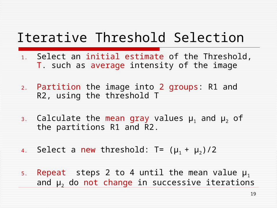
Variable Thresholding Another useful technique in the case of uneven

illumination

Approximate the intensity values of the image by a simple function such as a plane or biquadratic.

The fit function is determined by the gray value of the background.

Histogramming and thresholding can be done relative to the base level determined by the fitted function.

24

a: original imageb: 3-D plot c: histogramd: T = 85e: T= 165f: planar function( fit

between box & Background)

g: difference plot (a-f)h: the normalized

imagei: histogram of

normalized imagej: result T=110

25

Double Thresholding(1) Select two thresholds T1 and T2.(2) Partition the image into three regions :R1, containing all pixels with gray values below T1.R2 , containing all pixels with gray values between T1 and

T2 , inclusive.R3 , containing all pixels with gray values above T2. where R1=core region, R2 = fringe (intermediate,

transition) region, R3 =background.(3) Visit each pixel in region R2 . If the pixel has a neighbor

in region R1, then reassign the pixel to region R1.(4) Repeat step 3 until no pixels are reassigned.(5) Reassign any pixels left in region R2 to R3 .

26

(a). Original image(b). Histogram

(c). Core T1=70(d). Result after growing the

core using T2=155

(e).Regular Method T= T2

(f). Regular Method T1≤T≤T2

27

Limitation of Histograms

They are applied globally to the entire image. This can be a drawback in complex scenes.

Very useful in initial segmentation on the basis of gray levels.

Spatial information about intensity values is thrown away.

Very different scenes may give a strikingly similar

histogram representation.

Histogram for both images

28

Region Representation Different representations suitable to different

applications. Three general classes:- 1. Array representation - same size arrays, membership arrays 2. Hierarchical representation - pyramid, quad tree 3. Symbolic representation

29

Array representation Uses array of same size as original image with

entries indicating the region to which a pixel belongs.

Image Data

30

Membership Arrays Membership arrays (images) commonly

called masks. Each region has a mask that indicates which pixels belong to which region.

Advantage – a pixel can be allowed to be a member of more than one region.

31

• Preserves all details of regions required in most applications

• Very popular method with lots of hardware support available

• Symbolic information is not explicitly represented.

Characteristics of array representation method

32

Hierarchical Representation Images represented at many resolutions

As resolution , array size and some data is lost. More difficult to recover information.

But, memory and computation requirements are also decreased.

Used to accommodate various segmentation algorithms which operate at different resolutions.

33

Pyramids

An ‘n x n’ image represented by the image and ‘k’ reduced versions of the image.

Pixel at level ‘l’ has combined information from several pixels at level ‘l+1’

Top level – level 0 – single pixel

Bottom level – original image

Simplest method for resolution reduction is averaging.

34

Pyramid Structure

Averaging in 2*2 neighborhood

35

Quad Trees Extension of pyramids for binary images.

Three types of nodes – white, black, gray. White or black node – no splitting.

Gray node – split into 4 sub-regions.

Each node is either a leaf or has 4 children.

36

Quad Tree ExampleBinary Image

SW SE

NE

NW

NW

NE SE SW

37

Quad Tree ExampleNon-binary image

1122 3344

1122 3344

1122 3344

Not uniformNot uniform

uniformuniform

38

Symbolic Representations Commonly used symbolic characteristics: 1. Enclosing rectangle 2. Centroid 3. Moments 4. Euler number

5. Others: Mean, variance of intensity values

39

Data Structures for Segmentation

Data structures used for storing region information during operations like splitting and merging.

Commonly used data structures:- 1. RAG – Region Adjacency Graph 2. Picture trees 3. Super grid

40

RAG (Region Adjacency Graph) Nodes represent regions; arcs between

nodes represent a common boundary between regions.

Different properties of regions stored in node data structure.

After initial segmentation, results stored in RAG and regions combined to obtain a better segmentation.

41

RAG Example

42

Algorithm: Region Adjacency Graph

(1) Scan the membership array a and perform the following steps at each pixel index [i,j]

(2) Let r1 = a[i,j]

(3) Visit the neighbors [k,l] of the pixel at [i,j]. For each neighbor, perform the following:

(4) Let r2 = a[k,l] , if r1 != r2 , add an arc between nodes r1 and r2 in the region adjacency graph

43

Picture Trees Emphasize inclusion of a region within

another region.

Recursive splitting of an image into component parts. Splitting stops with constant characteristic conditions.

Quad tree is a special case.

44

Picture Tree Example

45

Super Grid Boundaries should be located between the pixels of

two adjacent regions.

However, often boundaries become actual pixels in image representations.

For NxN image, super grid will be (2N+1) x (2N+1).

Each pixel surrounded by 8 non-pixel points which are used to indicate boundary.

Simplifies merge and split operations.

46

Super grid Example

47

Split and Merge After segmentation the regions may need to be

refined or reformed. Split operation adds missing boundaries by splitting

regions that contain part of different objects. Merge operation eliminates false boundaries and

spurious regions by merging adjacent regions that belong to the same object.

48

Algorithm: Region Merging(1) Form initial regions in the image using thresholding

(or a similar approach) followed by component labeling.

(2) Prepare a region adjacency graph (RAG) for the image.

(3) For each region in an image, perform the following steps: (a) Consider its adjacent region and test to see if they

are similar. (b) For regions that are similar, merge them and modify

the RAG. (4) Repeat step 3 until no regions are merged.

49

similarity Approaches Determining similarity between two regions is most

important step.

Approaches for judging similarity based on:• Gray values

• Have the same mean intensity value• Have the same statistical distribution of intensity value

• Color• Texture• Size• Shape• Spatial proximity and connectedness

50

Region Merging A Statistical Approach

Assumption:- Regions have constant gray values corrupted by statistically independent, zero-mean Gaussian noise

Gray values are now taken from normal distributions. Suppose two adjacent regions R1 and R2 contain m1 and m2

points respectively. Possible hypotheses are: H0 : Both regions belong to same object. Intensities are all drawn

from a single Gaussian distribution with parameters H1: Regions belong to different objects. Intensities are drawn

from separate Gaussian distributions with parameters

These parameters are generally not know, but estimated using the available samples.

2211 ,,,

51

Statistical Approach (Continued) Assume a region contains n pixels having gray levels, gi,

i =1,2,….n with a normal distribution:

The Maximum Likelihood Estimation can be used to determine parameters like mean and variance.

2

2

2

2

1)(

gi

egip

52

Statistical Approach (Continued) Under H0, the joint probability density can be

found.

53

Statistical Approach (Continued) Similarly, under H1, assuming normal

distributions for regions R1 and R2, the joint probability density can be obtained.

54

Statistical Approach (Another slide!!) The likelihood ratio, L, is the defined as the ratio of the probability densities under the two

hypotheses:

If L < threshold T, strong likelihood that there is only one region and the two regions may be merged.

NOTE: Can also be applied for edge detection.

Modifications: Possible to assume planar or quadratic intensity distributions instead of constant gray values.

22

11

210

021

121

|,....,

)|,....,(mm

mm

Hggp

HggpL

55

Removing Weak Edgesfor Region Merging

Merge regions if boundary is weak.

Length of common boundary is considered.

Weak boundary – intensities of either side differ by less than amount T

Imp:- Consider relative lengths of the weak and complete boundaries between regions.

56

Removing Weak EdgesTwo main approaches

Approach 1. Merge adjacent regions R1 and R2 if W = length of weak part of boundary S = min(S1,S2) is minimum of two perimeters = a threshold If is too small too many region merges is big very conservative algorithm; valid candidates for

merging might be ignored. Good heuristic is 0.5

S

W

57

Removing edges (Continued)Approach 2. Merge adjacent regions R1 and R2 if

where S = common boundary W = length of weak part of boundary = threshold Good heuristic is 0.75

S

W

58

Region Splitting Property of a region is not constant - SPLIT Segmentation starts with large regions. Whole image can be

used to start with. Important decisions before splitting:- 1. Is a property not constant over a region? It is application dependant and requires knowledge about regions

like: - Variance of intensity values - Function fitting and error calculation

2. Where to split a region? - Finding best boundary for dividing (Measures of edge

strength within region). - Regular decomposition methods (divide in fixed equal region like

quad-tree)

59

Algorithm: Split and Merge Region Segmentation Start with the entire image as a single region

Split: Pick a region R. If H(R) is false, then split the region into four sub regions. H(R)=1 if the variance is small, 0 otherwise

Merge: Consider any two or more neighboring sub regions, R1, R2,…, Rn, in the image. If H(R1UR2U…Rn) is true, merge the n regions into a single region

Repeat these steps until no further splits or merges.

60

Region Growing

Group pixels or subregions into larger regions based on pre-defined data

Start with a set of ‘seed’ points

Check the neighboring pixels and add them to the region if they are similar to the seed

61

Application dependent for example: If targets need to be

detected using infrared images, choose the brightest pixel(s)

Without a priori knowledge, for example: compute the histogram and

choose the gray-level values corresponding to the strongest peaks

How to Choose Seeds

62

similarity criteria

based on any characteristic of the region in the image: Average intensity Variance Color Texture Motion Shape Size

63

Similarity Criteria for Region Growing

Satellite imagery – color

Monochrome images – Descriptors : Gray levels, moments, texture Connectivity or adjacency information

64

Example – Region Growing Fig. shows x-ray image of

a weld with defects and a histogram of the image.

Defects have max. value (255). All these point are used as seed regions.

65

Example (continued) Criteria for region

growing: Absolute gray level

difference less than 65.

Pixel 8-connected to at least one pixel in the region.

Figs. show seed points and results of region growing