Louisiana State University LSU Digital Commons LSU Master's eses Graduate School 2003 Regional water quality models for the prediction of eutrophication endpoints Anindita Das Louisiana State University and Agricultural and Mechanical College, [email protected] Follow this and additional works at: hps://digitalcommons.lsu.edu/gradschool_theses Part of the Environmental Sciences Commons is esis is brought to you for free and open access by the Graduate School at LSU Digital Commons. It has been accepted for inclusion in LSU Master's eses by an authorized graduate school editor of LSU Digital Commons. For more information, please contact [email protected]. Recommended Citation Das, Anindita, "Regional water quality models for the prediction of eutrophication endpoints" (2003). LSU Master's eses. 1496. hps://digitalcommons.lsu.edu/gradschool_theses/1496

Welcome message from author
This document is posted to help you gain knowledge. Please leave a comment to let me know what you think about it! Share it to your friends and learn new things together.
Transcript

Louisiana State UniversityLSU Digital Commons
LSU Master's Theses Graduate School
2003
Regional water quality models for the prediction ofeutrophication endpointsAnindita DasLouisiana State University and Agricultural and Mechanical College, [email protected]
Follow this and additional works at: https://digitalcommons.lsu.edu/gradschool_theses
Part of the Environmental Sciences Commons
This Thesis is brought to you for free and open access by the Graduate School at LSU Digital Commons. It has been accepted for inclusion in LSUMaster's Theses by an authorized graduate school editor of LSU Digital Commons. For more information, please contact [email protected].
Recommended CitationDas, Anindita, "Regional water quality models for the prediction of eutrophication endpoints" (2003). LSU Master's Theses. 1496.https://digitalcommons.lsu.edu/gradschool_theses/1496

REGIONAL WATER QUALITY MODELS FOR THE PREDICTION OF EUTROPHICATION ENDPOINTS
A Thesis
Submitted to the Graduate Faculty of the Louisiana State University and
Agricultural and Mechanical College In partial fulfillment of the
Requirements for the degree of Master of Science
in
The Department of Environmental Studies
by Anindita Das
B.S., University of Calcutta, 1991 December, 2003

ACKNOWLEDGEMENTS
I am extremely grateful to my major professor, Dr. E. Conrad Lamon III, for his
patience and guidance. He was always there to explain and give valuable suggestions for
the improvement of this thesis. I would also like to express my sincere appreciation to my
committee members, Dr. Walter K. Keithly, Dr. Michael Wascom and Dr. Margaret
Reams, for their support (course-related as well as moral) throughout the two years in this
department.
I would like to thank my husband, Neel Das, who has always stood by me and
was always there to reassure me when I was feeling disheartened. I am forever grateful to
my parents for being my pillar of strength and for encouraging me in all that I do. Thanks
also to my friends and family for their positive attitude, understanding and support.
ii

TABLE OF CONTENTS ACKNOWLEDGEMENTS ….…………………………………………………………...ii LIST OF TABLES…………………………………………………………………...……v LIST OF FIGURS………………………………………………………………………...vi ABSTRACT ………………………………………………………….…………………viii CHAPTER 1. INTRODUCTION…………………………………………………………1 CHAPTER2. EPA’S WATER QUALITY INVENTORY……………………………...6 Sources of Nutrient Pollution…………...…………………………………………7 Limiting Factors in Eutrophication……….…………………………..…………...9 CAHPTER 3. ESTABLISHING NUTRIENT CRITERIA……………………………...11 CHAPTER 4. DEVELOPMENT OF ECOREGIONS…………………………………..15 Formation of Nutrient Criteria Database ………………………………….……..16 Dealing with Quality of Historical Data.………………………………………...18 CHAPTER 5. MATERIALS AND METHODS………………………………………...21 Regression Criticism……………...……………………………………………...25 Residuals Used……………………...…………………………………………....26 Residual Analysis………………………………………………………………...27 Exploratory Data Analysis Techniques……………………………………….…28 CHAPTER 6. RESULTS………………………………………………………………...30 CHAPTER 7. DISCUSSION…………………………………………………………….44 Limitations of the Models…………………...………………………….………..44 Other Approaches………………………….……………………….…………….47 Summary/Conclusion……………………………………...………………..……48 REFERENCES……………………………………………………………….…………..52 APPENDIX A. CONSENT FORM…………….………………………………………..56 APPENDIX B. SAS ANOVA OUTPUT FOR MODELS……………………...……….59 APPENDIX C. TABLES WITH PARAMETER VALUES FOR EACH MODEL…….68 APPENDIX D. BOXPLOTS OF DISTRIBUTION OF CHLOROPHYLL A FOR EACH MODEL BY ECOREGION……………………………………………….73
iii

APPENDIX E. MAPS OF THE SPATIAL DISTRIBUTION OF OBSERVATIONS FOR EACH MODEL…...………………………………………..…77 APPENDIX F. SAS CODES………………………………….………………………….84 APPENDIX G. SUMMARY STATISTICS FOR ECOREGIONS………...……………96 VITA……………………………………………………………………………………120
iv

LIST OF TABLES
Table 1: Regression equations for TN..…..……………………………………………...22 Table 2: Total number of data and spatial spread of models.………….………………...24 Table 3: Comparison of the six models ….……………………………………………...42 Table 4: Weighted ranks of each model….……………………………………………...43
v

LIST OF FIGURES
Figure 1: Percentage of lakes assessed …...…….………………………………………...7 Figure 2: The bar charts, (a) and (b), present the leading sources and the number of lake, reservoir, and pond acres impacted ………………………………………………8 Figure 3: Fourteen nutrient Ecoregions as delineated by Omernik (2000)……..………..17 Figure 4: Summary plots of the residuals for Model 1.……...…………………………..31 Figure 5: Predicted chlorophyll a vs. residual plot for Model 1……..…………………..31 Figure 6: Cook’s Distance plot for Model 1……………………………………………..32 Figure 7: Summary plots of the residuals for Model 2…………………………………..33 Figure 8: Predicted chlorophyll a vs. residual plot for Model 2…..……………………..33 Figure 9: Cook’s Distance plot for Model 2……………………………………………..34 Figure 10: Summary plots of the residuals for Model 3…………………………………35 Figure 11: Predicted chlorophyll a vs. residual plot for Model 3..………………………35 Figure 12: Cook’s Distance plot for Model 3……………………………………………36 Figure 13: Summary plots of the residuals for Model 4…………………………………37 Figure 14: Predicted chlorophyll a vs. residual plot for Model 4..………………………38 Figure 15: Cook’s Distance plot for Model 4. ….………………………………………39 Figure 16: Summary plots of the residuals for Model 5…………………………………39 Figure 17: Predicted chlorophyll a vs. residual plot for Model 5..………………………40 Figure 18: Cook’s Distance plot for Model 5……………………………………………40 Figure 19: Summary plots of the residuals for Model 6…………………………………41 Figure 20: Predicted chlorophyll a vs. residual plot for Model 6…..……………………41 Figure 21: Cook’s Distance plot for Model 6……………………………………………42
vi

Figure 22: LogTKN vs. residual plot for Model 5.………………………………………50 Figure 23: LogTP vs. residual plot for Model 5…………………………………………50
vii

viii
ABSTRACT
Eutrophication is a process by which a waterbody progresses from its origin to its
extinction. During this period, there is a gradual accumulation of nutrients and organic
biomass, accompanied by a decrease in average depth of the water due to sediment
accumulation, and an increase in primary productivity, usually in the form of dense algal
blooms. Cultural eutrophication occurs when humans, through their various activities,
greatly accelerate this process. Eutrophication can cause loss in species diversity, fish
kills, and decrease the aesthetic value of a waterbody. The EPA is trying to prevent
cultural eutrophication by setting standards for water quality criteria for each of the
fourteen ecoregions in the United States. Nutrients are the most common pollutants
affecting waterbodies. The EPA considers total phosphorous and total nitrogen as the two
causal variables and chlorophyll a and Secchi depth as the two early indicator response
variables. There are models that predict the relationship of chlorophyll a to phosphorous
and chlorophyll a to nitrogen, but there are very few that combine phosphorous and
nitrogen to predict chlorophyll a at a cross-sectional level. This study is concerned with
fitting a linear model for the prediction of chlorophyll a, using phosphorous and nitrogen,
for the fourteen ecoregions. Six combinations of the three variables have been tested
(because of the different methods used to obtain each variable) to find out which model is
the best with respect to model fit, number of observations, and geographical coverage.
The best model can then be used in further studies to determine eutrophication end points
at smaller and more homogeneous divisions of the ecoregion for better management of
water quality in lakes.

CHAPTER 1. INTRODUCTION
Eutrophication is a process by which a waterbody progresses from its origin to its
extinction (Novotny and Olem, 1994). Natural eutrophication occurs over thousands of
years during which lakes gradually age and become more productive. During this period,
there is a gradual accumulation of nutrients and organic biomass, accompanied by a
decrease in average depth of the water due to sediment accumulation, and an increase in
primary productivity, usually in the form of dense algal blooms. These algal blooms
become the dominant species in the water body and overshadow the flora and fauna in
the deeper water column, leading to a loss of diversity.
The EPA characterizes as eutrophic waterbodies that have decreasing
hypolimnetic dissolved oxygen concentrations, increasing nutrient concentrations,
increasing suspended solids, especially organic material, progress from a diatom
population to a population dominated by blue-green or green algae, decreasing light
penetration, and increasing phosphorous concentrations in the sediments.
Cultural eutrophication occurs when humans, through their various activities,
greatly accelerate this process. This might be beneficial in some aquatic systems. For
example, in aquaculture, ponds are deliberately fertilized to increase the production of
fish or shellfish. In general, though, cultural eutrophication causes problems when the
increased production levels, and the effects associated with this, are not compatible with
the intended uses of the waterbody. This can drastically reduce the life span of a lake
through accelerated aging.
Cultural eutrophication affects the value of aquatic systems in three major ways.
First, the species associated with the eutrophic system are undesirable. For example, as
1

blue-green algae become more dominant due to nutrient enrichment, the fish species
present may be commercially less valuable, so, the monetary value of the waterbody
declines.
The second reason is that in highly eutrophic systems, oxygen concentrations vary
over a wide range due to increased productivity and plant biomass decomposition. Many
organisms cannot stand such fluctuations (which may result in fish kills). Large-scale fish
kills of desirable species are a serious problem associated with eutrophication.
Finally, increased phytoplankton populations (due to nutrient enrichment)
decrease the aesthetic value of water by making it appear turbid. Large plant biomasses
decay, creating a rotten smell. These may make a waterbody unsuitable for water supply,
contact recreation and navigation.
The Environmental Protection Agency’s (EPA) mandate is to protect the
country’s waters by setting standards for the management of water quality criteria in the
United States. Section 304 of the Clean Water Act deals with a scientific assessment of
ecological and human health effects recommended by EPA to the States and Tribes for
establishing water quality standards. These would serve as a basis for control of
discharges or release of pollutants (USEPA 2000). EPA intends to use this scientific
assessment to develop the default nutrient criteria in Section 304(a) of the Clean Water
Act for the all the ecoregions in the country. This process requires good policy, which
requires good science (Reckhow, 1994). But there are many uncertainties in science (e.g.,
natural variability, modeler bias, sampling bias, knowledge base, etc.). According to
Reckhow (1994), one way to approach this problem is to first build a decision planning
framework that identifies management objectives, attributes to calculate achievement of
2

those objectives, and plans that have to be executed to attain those objectives. This would
help in making management decisions, taking into account significant scientific
uncertainty.
For example, control of eutrophication might be a management objective. One
way to approach this is the control of algal blooms. Chlorophyll a is a surrogate measure
of the amount of algal biomass present in a waterbody. Phosphorous and nitrogen are
attributes that can be used to predict the amount of chlorophyll a present in a waterbody.
Chlorophyll a would be considered an attribute which can be used as a measure for
achieving an objective (control of eutrophication). The next step in the framework is to
define the type of scientific decision support to attain the objective. Decision support
includes predictive methods (e.g., expert judgments, simulation models) and information
needs (e.g., research, monitoring, experiments) (Reckhow, 1994).
In this regard, many models have been proposed, like WASP4 (Ambrose et al, 1988),
QUAL2E (Brown et al, 1987), EUTROMOD (Reckhow, 1992). Chlorophyll a is
considered a measure of eutrophication because the amount of chlorophyll a can be used
to estimate the amount of algal biomass present in a waterbody. Presence of phosphorous
and nitrogen are considered the primary causes of eutrophication (USEPA, 2000). There
are several models that deal with phosphorous and nitrogen loading (Vollenweider, 1969;
Portielje and Van der Molen, 1999). There are also models that predict the relationship of
chlorophyll a to phosphorous (Jones et al, 1998; Walker and Havens, 1995) and
chlorophyll a to nitrogen (De Vries et al, 1998; Mineeva, 1993), but there are very few
that combine phosphorous and nitrogen to predict chlorophyll a (Lamon, 1995; Lamon
3
and Clyde, 2000). This combination is important because taken together, these two
variables might be able to explain more variation in chlorophyll a in the waterbodies.
The Environmental Protection Agency (EPA) is endeavoring to set standards for
water quality criteria for each of the fourteen ecoregions (USEPA, 2002) in the United
States. The first step in addressing this issue is designing models required for decision
support. Data availability for these models is the next step. In this regard, EPA has
developed a Nutrient Criteria Database containing data for many variables as a beginning
point for development of models. However, these models also require consistency in
terms of the variables being used. For example, prediction of chlorophyll a from
phosphorous and nitrogen requires that all three variables be measured simultaneously in
all the observations and that each parameter be measured using a single method over time
(because it is recommended by EPA that data for the same variable cannot be
interchanged if they have been obtained by different methods).
This study is concerned with fitting a linear model for the prediction of
chlorophyll a using phosphorous and nitrogen as predictors, for the fourteen ecoregions
(recommended by EPA). The Nutrient Criteria Database will be assessed to find whether
or not it is consistent when it comes to using the same method for measuring a variable or
in measuring all the variables at the same time from a single sample of water. Six
combinations of the three variables mentioned above will be tested (because of the
different methods used to obtain each variable) to find out which model gives the best
estimate of chlorophyll a with respect to model fit, number of observations, and
geographical coverage. This can then be treated as a preliminary step in the scientific
decision support of the planning framework for management of eutrophication. The
4

5
sections that follow will discuss the EPA’s water quality inventory, development of
nutrient criteria, formation of ecoregions, materials and methods used, results, and
discussion.
CHAPTER 2. EPA’S WATER QUALITY INVENTORY
EPA’s ecoregional nutrient criteria (USEPA, 2000) address mainly cultural
eutrophication. The Clean Water Act states that all waters should be able to provide for
recreation and the protection and propagation of aquatic life. EPA sets water quality
standards to protect the nation’s waterbodies. EPA’s water quality standards have three
elements: designated uses, water quality criteria and antidegradation policy.
Designated uses include, but are not limited to, drinking water supply, fish
consumption, ground water recharge, wildlife habitat, shellfish harvesting and agriculture.
Each designated use has its own set of water quality criteria that must be met for the use
to be realized.
Water quality criteria may be either numeric or narrative. Numeric criteria are
used to establish thresholds for physical conditions, chemical concentrations, and
biological attributes required to support a beneficial or designated use. Narrative criteria
describe, instead of enumerate, conditions that must be maintained to support a
designated use. For example, a narrative criterion might be “Waters must be free of
substances that are toxic to humans, aquatic life, and wildlife” (National Water Quality
Inventory, EPA, 2000).
Antidegradation policies are narrative statements used to protect existing uses and
to prevent waterbodies from deteriorating, even if their water quality is better than the
“fishable” and “swimmable” goals of the Act (National Water Quality Inventory, EPA,
2000).
In 2000, EPA assessed 43% of the lakes in the United States. Of these, 45% were
declared impaired and 55% were declared unimpaired (Figure 1). According to the EPA
6

report, “The Quality of Our Nation’s Waters”, nutrients are the most common pollutants
affecting assessed lakes. Nutrient impairment is found in 22% of the assessed lakes and
contributes to 50% of reported water quality problems in impaired lakes (Figure 2(a)).
Figure 1: Percentage of lakes assessed. Source: National Water Quality Inventory, 2000 Report, EPA.1 Sources of Nutrient Pollution
There are many sources of nutrient pollution including agriculture, urbanization,
hydromodification, and urban runoff and storm sewers (Figure 2(b)). According to EPA,
agriculture is the leading source of pollution in assessed lakes. Agricultural pollution
problems affect 18% of the assessed lakes and contribute to 41% of reported water
quality problems in impaired lakes. The main factor that causes increased transport of
pollutants in agriculture is disturbing the soil by tillage. This greatly increases sediment
loss compared to undisturbed soils. As much as 90% of nutrient loss (phosphorous and
nitrogen) are associated with this sediment loss (Alberts, et al 1978). Nutrient losses
represent only a small percentage of applied fertilizers, but their addition as run-off into
water bodies greatly increases the effects of eutrophication. The resultant accumulation in
1 Copy of permission in Appendix A
7

(a)
(b)
Figure 2: The bar charts, (a) and (b), present the leading sources and the number of lake, reservoir, and pond acres impacted. The percent scales on the upper and lower x-axes of the bar chart provide different perspectives on the magnitude of the impact of these sources. The lower axis compares the acres impacted by the source to the total assessed acres. The upper axis compares the acres impacted by the source to the total impaired acres. Source: National Water Quality Inventory, 2000 Report, EPA.2 2 Copy of permission in Appendix A
8

surface waters can cause fishkills (like the recent fish kills in the university lakes
(Advocate, 2003).
Urbanization affects 8% of the assessed lake acres and 18% of the impaired lake
acres (EPA, 2000). It is considered to have caused the most adverse change in water
quality (Novotny and Olem, 1994). It modifies atmospheric composition, the hydrology
of the watershed, receiving streams and other waterbodies, and soil. Urbanization has
increased emission of wastes from a variety of sources like industries, households,
transportation, sewage conveyance and disposal (landfills and incinerators). Increased
imperviousness of soils decreases the capacity of the soil to store runoff water and this
tends to make runoff peak levels higher. Urbanization of watersheds increases
imperviousness of the soils making the surface flows peak at higher levels and also
increases the volume (Novotny and Olem, 1994).
Examples of hydromodification are flow regulation and modification,
channelization, dredging and construction of dams (which mainly affects rivers). This
modification changes the natural habitat in such a way that it can no longer support fish
and other desired flora and fauna.
In unsewered urban development, sewage is usually disposed into soils (e.g.,
septic tanks). When the adsorption capacity of this soil disposal system is exhausted,
nutrients enter ground water. But during storm runoff, the hydraulic load exceeds the
infiltration capacity and surface waters are contaminated by the sewage.
Limiting Factors in Eutrophication
It has been found, through various experiments, that the limiting factors in
primary production are nitrogen (Ryther and Dunstan, 1971) and phosphorous (Schindler,
9

10
1974). Generally, phosphorous is the limiting factor in fresh water systems and nitrogen
in marine systems (Laws, 1981). Phosphorous becomes the limiting factor because many
species of phytoplankton (e.g., blue-green algae) are capable of fixing atmospheric
nitrogen and so may compensate for nitrogen deficiency in the water. This is not possible
with phosphorous. All essential phosphorous has to come from outside inputs or sediment
recycling in the water body. Also, the negative phosphate ion (PO43-), forms insoluble
compounds with many positive ions like Al3+, Ca2+ and Fe3+, the main compound being
ferric phosphate. These sink to the bottom as precipitates, trapping phosphate in the
sediments, and hence make this phosphorous unavailable to the phytoplankton. In marine
systems, iron concentration is much lower than in fresh water and therefore precipitation
of ferric phosphate is not important in marine phosphorous cycles. Also, blue-green algae
are a small proportion of the phytoplankton population of marine systems, so nitrogen
fixation becomes less important.

CHAPTER 3. ESTABLISHING NUTRIENT CRITERIA
Trophic state variables comprise measures of nutrient concentration (like total
phosphorous, soluble reactive phosphorus, total nitrogen, total Kjeldahl nitrogen), plant
(macrophyte or algal) biomass (e.g., organic carbon, chlorophyll a, Secchi depth), and
watershed attributes like land use (USEPA, 2000). All of these could be used to establish
criteria to deal with eutrophication concerns, but only a few are feasible as candidates for
early warning variables. The factor that limits plant biomass may change seasonally or
over longer periods of time, vary depending on the land use, or vary regionally. So, it
does not make sense to construct a single nutrient criterion when that nutrient may not
necessarily limit a target lake or lakes. This is why EPA emphasizes the development of
nutrient criteria based on both the nutrient inputs (cause) and the biological response
(effect).
The EPA considers total phosphorous and total nitrogen as the two causal
variables and chlorophyll a and Secchi depth as the two early indicator response variables
among other variables like dissolved oxygen, macrophyte, benthic algal growth or
speciation, and other fauna and flora changes. The causal variables (phosphorus and
nitrogen) are necessary criteria because they will be the limits required to establish
management objectives and are usually directly related to discharge runoff abatement
efforts by the states. Dissolved oxygen is also an important parameter to be considered.
Dissolved oxygen is necessary for protecting aquatic life. This is especially important in
the case of fishes because different species of fishes have different oxygen tolerance
levels. However, nutrients have a marked but indirect effect on dissolved oxygen.
Increased levels of nutrients affect the dissolved oxygen balance by increased growth of
11

flora and decomposing biomass. Also, dissolved oxygen levels vary diurnally, and this
important variability is not likely to show up in monthly observations. In this study,
dissolved oxygen has not been considered.
Different forms of phosphorus can be measured to determine trophic state. Of
these, total phosphorus (TP) is a measure of all forms of dissolved or particulate
phosphorus in a sample. TP concentrations in runoff or areal exports can also be readily
related to watershed land use (Reckhow and Simpson, 1980; Walker, 1985a). This makes
it a superior variable for addressing point and nonpoint source loads from the watershed.
This is why TP has been used throughout North America as a basis for setting trophic
state criteria and in developing related models (NALMS, 1992), and the reason why it
was chosen as a causal variable in this thesis.
Control of nitrogen sources is more difficult than phosphorous because nitrogen
can be assimilated directly from the atmosphere by several types of organisms, including
some species of Cyanophyta (blue-green algae). Nitrogen is not as often limiting to plant
growth, thus the focus on phosphorous as the major factor considered in eutrophication.
The most common forms of nitrogen that are of concern in eutrophication
evaluation are nitrite, nitrate, ammonia, and organic nitrogen (as measured by total
Kjeldahl nitrogen (TKN)). Total nitrogen (TN) is considered to be the sum of ammonia,
nitrate, nitrite, and TKN. Usually, nitrate, nitrite, and ammonia are present at very low
levels in lakes or reservoirs unless there are some relatively recent loadings in runoff
from the watershed, or if nitrogen is not the limiting factor of algal growth in that
particular water body. These forms are rapidly used by algae and aquatic plants or
12

converted to other forms of nitrogen. The most useful measurement from a modeling
standpoint is either TN or TKN (USEPA, 2000).
Chlorophyll a is the major photosynthetic pigment in plants. It is an important
variable when one wants to estimate the photosynthetic capacity of an ecosystem. It is a
surrogate measure of algal density, which is costlier to measure. Therefore, it is the
chosen variable when an estimate of the primary productivity of an ecosystem is required.
Chlorophyll a is also preferred as an indicator because there are lakes where TP is not the
sole or primary limiter of algal production or biomass, for example, lakes with high
inorganic turbidity or high flushing rates (USEPA, 2000). The relationship between
chlorophyll and phosphorus and its linkage to algal biomass, makes chlorophyll a major
component of trophic state indices (Carlson, 1977) and water quality criteria.
In addition to the use of chlorophyll a in classification, the chlorophyll interval
frequency, or bloom frequency, have been predicted based on regression equations
developed by Walker (1985b) relating blooms to phosphorus. These chlorophyll a
intervals can be related to varying user perceptions of lake condition. The projected
frequency of these extreme events, as a result of increased phosphorus loading, can be
readily understood by citizens and decision-makers (Heiskary and Walker, 1988).
EPA encourages the development of mechanistic or empirical models for
identification of overenrichment problems, management planning, and determination of
status and trends of water resources. The causal and biological and physical response
variables represent only a set of starting points for States and Tribes to use in establishing
their own criteria. This is because control of causal variables would help to protect uses
before impairment occurs and to maintain downstream uses. Early response variables
13

14
would warn of possible impairment and help to integrate the effects of variable and
potentially unmeasured nutrient loads.

CHAPTER 4. DEVELOPMENT OF ECOREGIONS
The establishment of a single, national nutrient criteria for lakes is not a sensible
goal when one considers the significant variability of water bodies that exists across the
country in a variety of climates, geographic locations, and ecosystems. Individual lakes
and reservoirs are affected by varying degrees of development, and user perceptions of
water quality throughout the country can differ even over small distances (USEPA,
2000). Consequently, EPA bases its nutrient criteria development process on an approach
that takes into account the geographic differences in lakes across the country and uses a
classification system to explain those differences. The initial classification scheme used
by EPA is the ecoregion approach (Omernik, 1987, 1988, 1995).
EPA defines lakes as natural and artificial impoundments with a surface area
greater than 10 acres and a mean water residence time of 14 or more days. Man-made
lakes with the same characteristics are viewed as part of the same system. Reservoirs are
man-made lakes for which the primary purpose of the impoundment is other than
recreation (e.g., boating, swimming) or fishing, and the water retention time and water
body depth and volume vary widely. This definition of lakes has been used by EPA for
collecting data to set reference conditions for water quality in lakes.
EPA identified geographic divisions as part of a hierarchical classification
procedure with the purpose of grouping similar lakes together. Classification of lakes was
used in order to reduce the variability of lake-related measures (e.g., physical, biological,
or water quality variables) within classes and maximize the variability among classes.
This helps to group lakes together that under ideal conditions would have similar
characteristics (e.g., biological, ecological, physical). Classification was restricted to
15

those characteristics of lakes that are intrinsic, or natural, and are not the result of human
activities. Measures like size, maximum or mean depth, detention time, in lake
phosphorous and nitrogen, and shape are incorporated.
Ecoregions are a mapped classification system of ecological regions, that is,
regions with assumed relative homogeneity of ecological characteristics (Omernik,
1987). EPA has developed maps of ecoregions of the United States at various levels of
resolution and aggregation (Omernik, 1987). The most commonly used is the Level III
ecoregions, consisting of 79 ecoregions in the conterminous United States. Ecoregions
were based on analysis of the spatial coincidence in all geographic phenomena that are
the source of or indicate differences in ecosystem patterns. These phenomena consist of
geology, physiography, vegetation, climate, soils, land use, wildlife, and hydrology. The
relative importance of each characteristic varies among ecoregions regardless of the
hierarchical level (USEPA, 2000).
Level III ecoregions were aggregated to describe broad areas, which are generally
comparable in quality and types of ecosystems as well as in natural and anthropogenic
characteristics that have an effect on nutrients. A map of these ecoregion aggregations
was made for the National Nutrient Criteria Program (USEPA, 2000). This aggregation
resulted in fourteen ecoregions (Figure 3). The regions are meant to furnish a geographic
framework for guidance and reporting for the National Nutrient Criteria Program and can
form the basis for initial development of nutrient criteria.
Formation of Nutrient Criteria Database
The Nutrient Criteria Database contains data from STORET, the National
Eutrophication Survey (NES), the National Surface Water Survey (NSWS), the
16

Figure 3: Fourteen nutrient Ecoregions as delineated by Omernik (2000). Ecoregions were based on geology, land use, ecosystem type, and nutrient conditions. Source: EPA.3 3 Copy of permission in Appendix A
17

Environmental Monitoring and Assessment Program (EMAP), the Clean Lakes Program,
Volunteer Monitoring Programs, State Monitoring Programs, the U.S. Army Corps of
Engineers and other sources.
Dealing with Quality of Historical Data
The quality of older historical data sets is usually a problem because the data
quality is often unknown. This is because objectives, methods, and investigators may
have changed many times over the years. The most reliable data are those collected by a
single agency using the same protocol for a limited number of years. When “mining”
from large heterogeneous data repositories such as STORET, EPA investigators screened
data for acceptance considering a number of factors like location, variables and analytical
methods, laboratory quality control, collecting agencies, time period, index period and
representativeness.
Location
STORET data are georeferenced. These data can be used to select specific
locations or specific USGS hydrologic units. For selection of lakes within a geographic
region, it is important to know the underlying principle and methods of site selection by
the original investigators. This information may be included in STORET metadata.
Variables and Analytical Methods
Thousands of variables are recorded in STORET records. Each separate analytical
method yields a unique variable. Methods differ in accuracy, precision, and detection
limits, so, it is generally not sensible to mix methods in the same analysis. According to
EPA, selection of a particular “best” method may result in very few observations, so it
suggests that it may be prudent to select the most frequently used method in the database.
18

Laboratory Quality Control
Laboratory quality control data (blanks, spikes, replicates, known standards, etc.)
are normally not accounted in the larger data repositories. EPA suggests that it is more
cost-effective to accept or reject all data of the collecting agency or laboratory based on
overall confidence of their quality control. Sometimes, eliminating lower quality data can
be counterproductive, because the increase in variance caused by analytical laboratory
error may be negligible compared with natural variability or sampling error.
Collecting Agencies
STORET data identifies the agency that collected the data. Selecting data only
from particular agencies with known, reliable collection and analytical methods and
accepted quality reduces inconsistency due to unidentified quality problems.
Time Period
Long-term records are vitally important for detecting and establishing trends.
While defining reference conditions for nutrient criteria, it is important to determine if
trends exist in the reference site database. For example, over time, many lakes may have
improved markedly while other lakes, exposed to increased nonpoint-source runoff, may
have declined in overall quality.
Index Period
An index period for approximating average concentrations should be designated if
nutrient and water quality variables were measured more than once a year. The index
period could represent the entire year, spring or fall mixing or the summer growing
season. The most suitable index period can be determined by investigators who should
consider the characteristics of the lakes of the region, the quality and quantity of data
19

20
available, and estimates of temporal variability (if available) (Nutrient Criteria Technical
Guidance Manual, EPA, 2000).
Representativeness
Historical data may have been collected for specific purposes, such as developing
nutrient budgets for eutrophic lakes. These data are not likely to be characteristic of the
type of region or lake of interest. The investigator has to decide whether the lakes in the
database are representative of the population of lakes to be characterized. If a sufficient
sample of representative lakes (i.e., one large enough to characterize reference
conditions) cannot be found, a new survey will be necessary (Nutrient Criteria Technical
Guidance Manual, EPA, 2000).

CHAPTER 5. MATERIALS AND METHODS
Data for the study were obtained from the Nutrient Criteria Database of the EPA.
The data were collected by state. Datasets from each state were then formatted in Access.
These were then merged to form a single dataset and then sorted by ecoregion. SAS and
S-PLUS were used in the analysis of this single dataset.
The Nutrient Criteria Database has observations for a large number of parameters
(Appendix G). Of these, the parameters of choice were Chlorophyll a Fluorometric
corrected (CHLA, ug/l, STORET code 32209) and Chlorophyll a Trichomatic
uncorrected, (CHLAtri, ug/l, STORET code 32210), total phosphorous (TP, ug/l,
STORET code 00665), total nitrogen (TN, mg/l, STORET code 00600) and Kjeldahl
nitrogen (TKN, mg/l, STORET code 00625). These parameters were chosen because they
were also used by EPA to formulate reference conditions for lakes.
This dataset has 593,650 observations. TP is present in only 324,325 samples, TN
in 163,838 samples, TKN in 91400 samples, CHLA in 15,816 samples, and CLHAtri in
79,572 samples. Since, in a linear model observations of all variables have to be present
simultaneously, only 93,894 samples could be used in the study. The ecoregions did not
have equal number of samples (Appendix G).
It was found that only three ecoregions (2, 7, and 8) had observations for total
nitrogen and total phosphorous with corresponding chlorophyll a (STORET code 32209)
observations (Appendix C). Also, only three ecoregions (9, 12, and 13) had observations
for total nitrogen and total phosphorous with corresponding chlorophyll a (STORET code
32210) observations (Appendix C). Total nitrogen consists of Kjeldahl nitrogen, nitrate
21

and nitrite. So, total nitrogen was regressed with total Kjeldahl nitrogen to find the extent
to which total nitrogen can be predicted using Kjeldahl nitrogen.
It was found that Kjeldahl nitrogen can account for 94.58% of total nitrogen
variability. Separate regressions were fit for each of the ecoregions mentioned above. The
equations used are given in Table 1. This was done in the above five ecoregions because
only in these was TN measured concurrently with TKN. Such a strong correlation
prompted the creation of a new parameter named “newTN”. This included all the actual
total nitrogen measurements along with the total nitrogen predicted from TKN in the
cases where TN was missing but TKN was present. This allowed an increase in the
number of observations and an increase in the spatial coverage. The relationship between
chlorophyll a with total phosphorous and total nitrogen is fit using log-log regression
models to stabilize the variance (Lamon, 1995). This is a common procedure in many
research fields and is usually the first analytical step (Hamilton, 1992; Reckhow, 1988).
Table 1: Regression equations for TN
Ecoregion Equation (Standard Error)
2 logTN = -0.445172475 + 0.766388167*(logTKN) (0.077) (0.095)
7 logTN = 0.000667036 + 0.991866474*(logTKN) (0.004) (0.019)
11 logTN = 0.047977207 + 1.0255552479*(logTKN) (0.010) (0.029)
12 logTN = 0.015506943 + 0.958164113*(logTKN) (0.001) (0.003)
13 logTN = 0.026786063 + 0.997622084*(logTKN) (0.001) (0.004)
As with any linear model, the observations to be analyzed had to have all three
variables as non-missing. Also, it was found that all the variables were not available for
22
all the ecoregions. Choosing just CHLA, TP and TN covered very few ecoregions (as
mentioned above). So, various combinations of the five parameters stated above were
made to find which combination of the three parameters (response and two predictors)
had the most observations, the most spatial coverage, and the best fit.
The combinations of the five parameters produced six datasets. These datasets
were analyzed, using regression, to find the best model defined by the three criteria
(model fit, number of observations and spatial coverage). The six models for these
datasets are given in Table 2.
The null hypothesis for these models is:
H0 : There is no significant variation in chlorophyll a due to the factors ecoregion,
total phosphorous and total nitrogen. In other words,
H0 : β0 = β1 = β2 = 0.
The alternative hypothesis or Ha is that at least one of the βs is non zero, or, there is some
variation in chlorophyll a due to ecoregion, total phosphorous and total nitrogen.
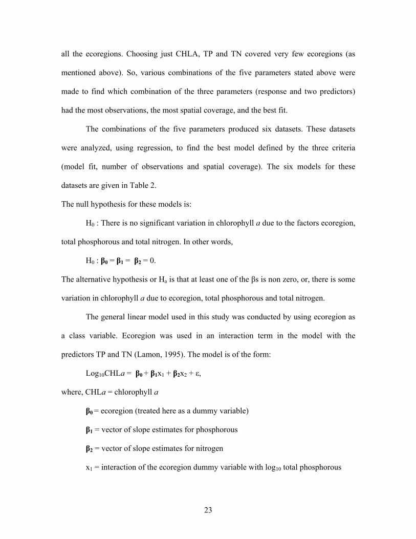
The general linear model used in this study was conducted by using ecoregion as
a class variable. Ecoregion was used in an interaction term in the model with the
predictors TP and TN (Lamon, 1995). The model is of the form:
Log10CHLa = β0 + β1x1 + β2x2 + ε,
where, CHLa = chlorophyll a
β0 = ecoregion (treated here as a dummy variable)
β1 = vector of slope estimates for phosphorous
β2 = vector of slope estimates for nitrogen
x1 = interaction of the ecoregion dummy variable with log10 total phosphorous
23

x2 = interaction of the ecoregion dummy variable with log10 total nitrogen
ε = residual
A dummy variable is a numerical variable (usually 0 and 1) used in a regression
analysis to represent subgroups of a sample. In this study, ecoregion has been used as a
dummy variable because it helps in using a single regression equation to represent
different ecoregions in each model.
In regression, a simple fit statistic, the coefficient of determination (R2) gives the
proportion of the variance of Y explained by regression on X. R2 is the explained
variance divided by total variance or 1- (residual variance/total variance). It ranges from
zero to one. Zero means no variance is explained, and one means hundred percent of the
variance is explained.
Table 2: Total number of data and spatial spread of models. _______________________________________________________________________ Models Total (N) # Ecoregions______________ Model 1 logCHLA = logTP + logTN 4246 3 2, 7, 8 Model 2 logCHLA = logTP + logTKN 5069 7 1, 2, 7, 8, 9, 11, 14 Model 3 logCHLA = logTP + lognewTN 4817 4 2, 7, 8, 11 Model 4 logCHLAtri = logTP + logTN 49301 3 9, 12, 13 Model 5 logCHLAtri = logTP + logTKN 20681 10 2, 3, 6, 7, 8, 9, 10, 11, 12, 13 Model 6 logCHLAtri = logTP + lognewTN 62475 6 2, 7, 9, 11, 12, 13 _______________________________________________________________________
Ordinary Least Squares (OLS) was used for regression analysis because it is one of
the most frequently used techniques for such analysis. This produces coeffiecient
estimates that minimize the sum of squared residuals. The solution obtained through OLS
assures “best fit” to the data. OLS works under some assumptions:
1. Fixed X: Theoretically, we can obtain many random samples, each with same X
values but different Yi due to different residual values.
24

2. Errors have zero mean. These two assumptions together ensure independence of
errors and X variables. This is sufficient for unbiased estimation of all parameters.
3. Errors have constant variance (homoscedasticity). Heteroscedasticity leads to
inefficiency and biased standard error estimates.
4. Errors are uncorrelated with each other. (No autocorrelation).
5. Errors are normally distributed. Nonnormal errors increase inefficiency and
undermine the rationale for t-tests and F-tests, especially with small samples. Also,
since OLS tends to track outliers, heavy-tailed error distributions can cause great
sample-to-sample variation.
Regression Criticism
Residuals versus predicted plots provide a starting point for criticism in multiple
regression. These may uncover problems such as curvilinearity, heteroscedasticity,
nonnormality, or outliers.
The linear model assumptions (i.i.d.) imply certain characteristics of the model error
term (the model residuals):
• Errors have identical distributions, with zero mean and same variance, for every
value of x.
• Errors are independent. They are unrelated to other errors, variables or cases.
• Errors are normally distributed.
Some possible violation of assumptions of regression are:
• Nonlinear relationships: Ordinary least squares (OLS) finds the best fitting
straight line, but this would be misleading if Y is actually a nonlinear function of
X.
25

• Nonconstant error variance: i.e., heteroscedasticity, when present, can lead to
misrepresentation of findings (over/under estimation) and thereby increase the
possibility of a Type I error.
• Correlation among errors: The standard errors, tests, and confidence intervals
assume independence among errors. But this might not always be the case,
especially when observations are adjacent in time and space. Correlation among
the errors could mean that there are effectively fewer observations than the
original dataset and this can lead to overestimation of the standard error and the
confidence intervals.
• Nonnormal errors: F and t tests assume normal distribution of errors. Nonnormal
errors may nullify these tests and increase sample-to-sample variation of the
estimates.
• Influential cases: OLS regression is not resistant; a single influential observation
can pull the regression line up or down and substantially influence all results.
Residuals Used
In the Jackknife procedure, n-1 cases of the dataset are used for calibration and
one case is used for confirmation of normality. This procedure is run n times, so each
case is used as a confirming case. If the confirmation is successful according to a
statistical goodness of fit criterion, then all of the data are used for the final calibration. In
this procedure, the model and parameter errors are better characterized because these
errors may be estimated by the net result of the “one-case-at-a-time” confirmation
(Rechow and Chapra, 1983).
26

A Studentized residual is a residual which has been divided by its estimated
standard error. This standard error is based upon fitting a statistical model using all points
except the point whose residual is to be computed. It is assumed that the residuals are
normally distributed, so these values approximately follow a t distribution, where for
large samples about 65% are between -1 and +1, about 95% are between -2 and +2, and
about 99% are between -2.6 and +2.6.
Residual Analysis
Testing regression assumptions focuses on errors (residuals) to measure their
plausibility. Residuals versus predicted values are a general-purpose diagnostic tool.
These plots can show an influential case, a curvilinear relation, a nonnormal residual
distribution and heteroscedasticity. Mean-median comparison provides a simple check for
symmetry, a necessary condition for normality. The mean OLS residual always equals
zero or is very close to zero. A non-zero median would then imply skewness.
The residuals of each model were also checked to ensure that they met the criteria for
other linear model assumptions (normal i.i.d).
Compliance with these assumptions is determined by graphical methods (e.g., plots of
residuals versus predicted values) and statistical tests (e.g., Kolmogorov-Smirnov test)
applied to the model residuals. The sum of squared residuals (RSS) reflects the overall
accuracy of predictions. The lower the RSS, the closer the fit. Another indication of
goodness of fit is the residual standard deviation, se. This measures scatter or spread
around a regression line.
The Kolmogorov-Smirnov test is a nonparametric test for goodness of fit. It does not
assume a normally distributed population. It compares the empirical distribution of a
27

variable with a normal distribution that has the same mean and variance as the empirical
distribution. The null hypothesis here is that the parameter has a standard normal
distribution. This test is very sensitive to violations of normality in the tails.
Cooks distance (Di) is a measure of influence. It measures influence on the whole
model. The value of Di is an indication of the ith case’s influence on all the estimated
regression coefficients. Two criteria for Di are:
• An observation is influential if Di > 1.
• An observation is extremely influential if Di > 4/n.
Exploratory Data Analysis Techniques
Boxplots are useful for a comparison between two or more distributions. They
provide information about the central tendency, given by the median, dispersion, which is
given by the interquartile range, symmetry and outliers (Appendix D).
A symmetry plot graphs the distance of the ith value of a dataset above the
median to the ith value below the median. Each pair of observation defines one point on
the plot. A symmetry plot of n data contains n/2 points. If the distribution were
symmetrical, the points would lie on one line. Points that do not lie on the line indicate
asymmetry. Positive skew is indicated if points lie above the line and negative skew is
indicated if points lie below the line.
Quantile-quantile plots are used to graph quantiles of one variable against another
variable. This can be used to compare two empirical distributions, or an empirical
distribution with a theoretical distribution (Hamilton, 1992). The latter is called a quantile
–normal plot or normal probability plot when variables are plotted against a Gaussian
28

29
distribution that has the same mean and standard deviation as the sample. Quantile-
normal plots of sample residuals can also help detect nonnormality.

30
CHAPTER 6. RESULTS
In all the six models, the p-value for the F-statistic is less than 0.0001 (Appendix
B), so we reject the null hypothesis and can say that at least one of the âs is non zero, or,
there is some variation in chlorophyll a explained by regression on total phosphorous and
total nitrogen.
Model 1 includes observations from only three ecoregions (2, 7, and 8). It
explains about 28% of the variation in chlorophyll a (Appendix B). The interaction effect
is significant (p< 0.0001), i.e., at least two of the ecoregions have different slopes or
intercepts. Tests for normality (Kolmogorov-Smirnov test) on the residuals show that as a
whole, the model residuals are not normal (p<0.01), as also seen in the difference
between the mean (0.0001) and the median (0.043). Visually, the summary plots (Figure
4) show a high degree of normality, except in the tails. The scatter plots (Figure 5) of the
predicted variable, chlorophyll a, versus the residuals, also show a random distribution.
Therefore, considering the number of observations (4246) used in the model, and the fact
that the Kolmogorov-Smirnov test is very sensitive in the tails, we can say that the
distribution is approximately normal. The Cook’s distance graph (Figure 6) also shows
that the values are well below 1, so there are no unduly influential observations.
Model 2 includes observations from seven ecoregions (1, 2, 7, 8, 9, 11 and 14). It
explains about 23% of the variability in chlorophyll a (Appendix B). ). The interaction
effect is significant (p< than 0.0001), i.e., at least two of the ecoregions have different
slopes or intercepts. Tests for normality (Kolmogorov-Smirnov test) on the residuals
show that as a whole, the model residuals are not normal (p<0.01), as also seen in the
difference between the mean (-0.00008) and the median (0.13). Visually, the summary

31
-2 -1 0 1 2
0.0
0.5
1.0
1.5
residuals(test.lm)
-2-1
01
Boxplot
resi
dual
s(te
st.lm
)Distance below median
Dis
tanc
e ab
ove
med
ian
0.0 0.5 1.0 1.5 2.0
0.0
0.5
1.0
1.5
Quantiles of Normalre
sidu
als(
test
.lm)
-1.0 -0.5 0.0 0.5 1.0
-2-1
01
Figure 4: Summary plots of the residuals for Model 1.
Predicted
Res
idua
l
-0.5 0.0 0.5 1.0
-2-1
01
Figure 5: Predicted chlorophyll a vs. residual plot for Model 1.

32
Coo
k's
Dis
tanc
e
0 1000 2000 3000 4000
0.0
0.02
0.04
0.06
0.08
541
4225
667
Figure 6: Cook’s Distance plot for Model 1.
plots (Figure 7) show a high degree of normality, except in the tails. There is a slight
negative skew. The scatter plots (Figure 8) of the predicted variable, chlorophyll a, versus
the residuals, also show a random distribution. Therefore, considering the number of
observations (5069) used in the model, and the fact that the Kolmogorov-Smirnov test is
very sensitive in the tails, we can say that the distribution is approximately normal. The
Cook’s distance graph (Figure 9) also shows that the values are well below 1, so there are
no unduly influential observations.
Model 3 includes observations from four ecoregions (2, 7, 8 and 11). It
explains about 27% of the variability in chlorophyll a (Appendix B). The interaction
effect is significant (p< 0.0001), i.e., at least two of the ecoregions have different slopes
or intercepts. Tests for normality (Kolmogorov-Smirnov test) on the residuals show that
as a whole, the model residuals are not normal (p<0.01), as also seen in the difference

33
-2 -1 0 1 2
0.0
0.4
0.8
1.2
residuals(test.lm)
-1.5
-0.5
0.5
Boxplot
resi
dual
s(te
st.lm
)
Distance below median
Dis
tanc
e ab
ove
med
ian
0.0 0.5 1.0 1.5
0.0
0.4
0.8
1.2
Quantiles of Normal
resi
dual
s(te
st.lm
)
-2 -1 0 1 2
-1.5
-0.5
0.5
Figure 7: Summary plots of the residuals for Model 2.
Predicted
Res
idua
l
0.0 0.5 1.0 1.5
-1.5
-1.0
-0.5
0.0
0.5
1.0
1.5
Figure 8: Predicted chlorophyll a vs. residual plot for Model 2.

34
Coo
k's
Dis
tanc
e
0 1000 2000 3000 4000 5000
0.0
0.00
20.
004
0.00
60.
008
42884195
3452
Figure 9: Cook’s Distance plot for Model 2.
between the mean (0.0001) and the median (0.030). Visually, the summary plots (Figure
10) show a high degree of normality, except in the tails. The scatter plots (Figure 11) of
the predicted variable, chlorophyll a, versus the residuals, also show a random
distribution. Therefore, considering the number of observations (4817) used in the model,
and the fact that the Kolmogorov-Smirnov test is very sensitive in the tails, we can say
that the distribution is approximately normal. The Cook’s distance graph (Figure 12) also
shows that the values are well below 1, so there are no unduly influential observations.
Model 4 includes observations from 3 ecoregions (9, 12 and 13). It explains about
60% of the variability in chlorophyll a (Appendix B). The interaction effect is significant
(p< 0.0001), i.e., at least two of the ecoregions have different slopes or intercepts. Tests
for normality (Kolmogorov-Smirnov test) on the residuals show that as a whole, the
model residuals are not normal (p<0.01), as also seen in the difference between the mean
(-0.00001) and the median (0.08). Visually, the summary plots (Figure 13) show a high

35
-2 -1 0 1 2
0.0
0.5
1.0
1.5
chlatpnewtn.3$res
-10
1
Boxplot
chla
tpne
wtn
.3$r
es
Distance below median
Dis
tanc
e ab
ove
med
ian
0.0 0.5 1.0 1.5
0.0
0.5
1.0
1.5
Quantiles of Normal
chla
tpne
wtn
.3$r
es
-1.0 -0.5 0.0 0.5 1.0
-10
1
Figure 10: Summary plots of the residuals for Model 3.
Predicted
Res
idua
l
-0.5 0.0 0.5 1.0
-10
1
Figure 11: Predicted chlorophyll a vs. residual plot for Model 3.

36
Coo
k's
Dis
tanc
e
0 1000 2000 3000 4000 5000
0.0
0.01
0.02
0.03
0.04
0.05
0.06
995
4796
1121
Figure 12: Cook’s Distance plot for Model 3.
degree of normality, except in the tails. The scatter plots (Figure 14) of the predicted
variable, chlorophyll a, versus the residuals, also show a random distribution. Therefore,
considering the number of observations (49301) used in the model, and the fact that the
Kolmogorov-Smirnov test is very sensitive in the tails, we can say that the distribution is
approximately normal. The Cook’s distance graph (Figure 15) also shows that the values
are well below 1, so there are no unduly influential observations.
Model 5 includes observations from 10 ecoregions (6, 7, 8, 9, 10, 11, 12 and 13).
It explains about 48% of the variability in chlorophyll a (Appendix B). The interaction
effect is significant (p< 0.0001), i.e., at least two of the ecoregions have different slopes
or intercepts. Tests for normality (Kolmogorov-Smirnov test) on the residuals show that
as a whole, the model residuals are not normal (p<0.01), as also seen in the difference
between the mean (-0.00002) and the median (0.11). Visually, the summary plots (Figure
16) show a high degree of normality, except in the tails. The scatter plots (Figure 17) of

37
the predicted variable, chlorophyll a, versus the residuals, also show a random
distribution. Therefore, considering the number of observations (20,681) used in the
model, and the fact that the Kolmogorov-Smirnov test is very sensitive in the tails, we
can say that the distribution is approximately normal. The Cook’s distance graph (Figure
18) also shows that the values are well below 1, so there are no unduly influential
observations.
-3 -2 -1 0 1 2 3
0.0
0.5
1.0
1.5
chlatritptn.4$res
-2-1
01
Boxplot
chla
tritp
tn.4
$res
Distance below median
Dis
tanc
e ab
ove
med
ian
0.0 0.5 1.0 1.5 2.0 2.5
0.0
0.5
1.0
1.5
Quantiles of Normal
chla
tritp
tn.4
$res
-1.5 -1.0 -0.5 0.0 0.5 1.0 1.5
-2-1
01
Figure 13: Summary plots of the residuals for Model 4.
Model 6 includes observations from 6 ecoregions (2, 7, 9, 11, 12 and 13). It
explains about 58% of the variability in chlorophyll a (Appendix B). The interaction
effect is significant (p< 0.0001), i.e., at least two of the ecoregions have different slopes
or intercepts. Tests for normality (Kolmogorov-Smirnov test) on the residuals show that
as a whole, the model residuals are not normal (p<0.01), as also seen in the difference
between the mean (-0.00001) and the median (0.08). Visually, the summary plots (Figure

38
19) show a high degree of normality, except in the tails. The scatter plots (Figure 20) of
the predicted variable, chlorophyll a, versus the residuals, also show a random
distribution. Therefore, considering the number of observations (62,475) used in the
model, and the fact that the Kolmogorov-Smirnov test is very sensitive in the tails, we
can say that the distribution is approximately normal. The Cook’s distance graph (Figure
21) also shows that the values are well below 1, so there are no influential observations.
Models 1, 2, and 3 represent many common ecoregions (Table 3). Model 1 has a
low R2 and a small N compared to models 4, 5 and 6. Model 2 has an even lower R2 and
larger root mean square error, and the number of observations representing each
ecoregion in this model is much less than to Model 1 and 3. Model 3 has a slightly lower
R2 than Model 1. Addition of the predicted TN (model 3) adds another ecoregion that is
represented by this model and also increases the proportion of TN that can explain
variation in chlorophyll a. So, based on R2 and root mean square error, Model 3 is a better
model than Model 1 or 2.
Predicted
Res
idua
l
0.0 0.5 1.0 1.5 2.0 2.5
-2-1
01
Figure 14: Predicted chlorophyll a vs. residual plot for Model 4.

39
Coo
k's
Dis
tanc
e
0 10000 20000 30000 40000 50000
0.0
0.00
10.
002
0.00
30.
004
28213
2376
38311
Figure 15: Cook’s Distance plot for Model 4.
-4 -2 0 2 4
0.0
0.5
1.0
1.5
chlatritptkn.5$res
-3-2
-10
1
Boxplot
chla
tritp
tkn.
5$re
s
Distance below median
Dis
tanc
e ab
ove
med
ian
0 1 2 3
0.0
0.5
1.0
1.5
Quantiles of Normal
chla
tritp
tkn.
5$re
s
-1.5 -1.0 -0.5 0.0 0.5 1.0 1.5
-3-2
-10
1
Figure 16: Summary plots of the residuals for Model 5.

40
Predicted
Res
idua
l
-0.5 0.0 0.5 1.0 1.5 2.0 2.5
-3-2
-10
1
Figure 17: Predicted chlorophyll a vs. residual plot for Model 5.
Coo
k's
Dis
tanc
e
0 5000 10000 15000 20000
0.0
0.00
20.
004
0.00
60.
008
5672
1391216327
Figure 18: Cook’s Distance plot for Model 5.

41
-4 -2 0 2 4
0.0
0.5
1.0
1.5
residuals(test.lm)
-3-2
-10
1
Boxplot
resi
dual
s(te
st.lm
)
Distance below median
Dis
tanc
e ab
ove
med
ian
0.0 0.5 1.0 1.5 2.0 2.5 3.0
0.0
0.5
1.0
1.5
Quantiles of Normal
resi
dual
s(te
st.lm
)
-1.5 -1.0 -0.5 0.0 0.5 1.0 1.5
-3-2
-10
1
Figure 19: Summary plots of the residuals for Model 6.
Predicted
Res
idua
l
-0.5 0.0 0.5 1.0 1.5 2.0 2.5
-3-2
-10
1
Figure 20: Predicted chlorophyll a vs. residual plot for Model 6.

42
Coo
k's
Dis
tanc
e
0 10000 20000 30000 40000 50000 60000
0.0
0.00
10.
002
0.00
30.
004
21299
57526
527
Figure 21: Cook’s Distance plot for Model 6.
Table3: Comparison of the six models.
Model R2 Root MSE logCHLA/tri (mean)
No. of Observa-tions (N)
No. of ecoregions
1 0.280531 0.323859 0.585787 4246 3 2 0.230490 0.492696 0.848403 5069 7 3 0.274044 0.344937 0.574107 4817 4 4 0.607496 0.336146 0.967883 49301 3 5 0.480209 0.365508 1.146313 20681 10 6 0.583141 0.347155 0.994776 62475 6
Model 4 has the largest R2 but it is represents observations from only 3 ecoregions
(9, 12 and 13). As seen in the map (Appendix E), data are restricted to Florida. Model 5
has a slightly lower R2 and a slightly higher root mean square error compared to Model 4,
but it has the largest spatial coverage (10 ecoregions). Of these 10 ecoregions, 3
ecoregions (2, 3 and 10) are under-represented in terms of number of observations
(Appendix C). Model 6 has an R2, a root mean square error and a spatial coverage of

43
ecoregions in between models 4 and 5. For models 4, 5 and 6, observations are dominated
by ecoregions 12 and 13.
The R2, number of observations, and number of ecoregions covered by each
model were ranked from highest to lowest (Table 4). Weights were assigned to them. R2
and number of observations were given equal weights of 0.25. The number of ecoregions
was assigned a weight of 0.5. This was given twice the weight of the others because it
will be useful for EPA to use a model that has the most coverage by ecoregion to set
nutrient criteria standards for the ecoregions so that these can be used as a guide by States
and Tribes to set their own standards.
Table 4: Weighted ranks of each model.
Model Rank of R2
(assigned weight = 0.25)
Rank of Number of Observations (assigned weight
= 0.25)
Rank of Number of Ecoregions (assigned
weight = 0.5)
Weighted Average
Rank
1 4 6 5 5 2 6 4 2 3.5 3 5 5 4 4.5 4 1 2 5 3.25 5 3 3 1 2.0 6 2 1 3 2.25
The weighted average rank for Model 5 ranks the lowest (2.0) and seems to be the
best model among the six models because it has a moderately large R2 (third of six), it
can be used to predict chlorophyll a in ten ecoregions (first of six), and has a large
number of observations (third of six). If equal weights were assigned to each of the
criteria, then model 6 ranks the highest.

CHAPTER 7. DISCUSSION
Statistical analysis and a deterministic approach are among the many approaches
that can be used to predict a dependent variable with respect to changes in independent
variables. In a deterministic approach, all pertinent knowledge about the independent
variables is considered in the model to predict the change in the dependent variable.
Results can be obtained as probabilities when uncertainties (like natural variability and
sampling bias) are taken into account. But this cannot account for uncertainties that are
unknown or less understood (e.g., model specifications). In contrast, statistical analysis
can be used to find confidence limits thus making an allowance for all these uncertainties.
But such analysis requires sufficient data of adequate quality (Portielje and Van der
Molen, 1999). Also, statistical analyses can at least quantify uncertainties, whereas the
deterministic approach needs other approaches, like Monte Carlo simulation, to account
for uncertainty. Regression analysis is a type of statistical analysis and has been used for
determining chlorophyll a levels from phosphorous and nitrogen for a cross-sectional
dataset (Reckhow, 1988). Using regression helps to explain some of the variability seen
in chlorophyll a levels in the lakes and can thus provide valuable information for
managing eutrophication.
Limitations of the Models
Scale should not be disregarded while making predictions from cross-sectional
models (Jones et al, 1998). Data used to fit the models have come from individual
samples taken from different monitoring stations in different lakes throughout an
ecoregion. The analysis of the data has been done at the spatial scale of an ecoregion. The
models can be treated as a basis for predicting chlorophyll a in individual lakes within an
44

ecoregion. But there may be spatial variability among the lakes within an ecoregion due
to size, morphology, land use patterns, latitude and longitude etc., and scaling up from
individual lakes to ecoregion might make the predicted chlorophyll a unsable for a single
lake within the ecoregion (i.e., the prediction uncertainty might be unacceptable for a
single lake within an ecoregion). This uncertainty or risk would have to be quantified
using a utility function (at the management level) to decide whether a model can be used
for decision making purposes.
There are many factors that may affect the amount of chlorophyll a in lakes, other
than nitrogen and phosphorous. Land use patterns, seasonality, depth, hydraulic retention
time, mixing, latitude (Dodds et al, 2002), zooplankton grazing, species organization of
the algal community, higher trophic levels and distribution of submerged macrophytes
(Portielje and Van der Molen, 1999) may all affect chlorophyll a. If these had been
incorporated into the model, more of the variability in the chlorophyll a may have been
explained. These predictors were not included in the present study because these
measurements would have to be concurrent with chlorophyll a in the dataset (Appendix
G) to be used in a regression. This was not the case in the Nutrient Criteria Database.
Also, including all these predictors might decrease the number of observations. This was
also the reason why Dodds et al (2002) could not construct more complex predictive
regression models using multiple variables in their study of benthic algal biomass
relations to nutrients in streams.
There is natural variability among lakes. Lakes in the same ecoregion might not
have the same attributes because delineation of ecoregions is not solely based on lake
attributes (e.g., size, morphology, geographic location, hydraulic residence time), but on
45
potential natural vegetation, physiography, soils and land use and land cover (Jennerette
et al, 2002). Therefore, the deviation from normality in the tails may be due to
heterogeneity in the data which could be a function of choosing ecoregion as a
geographic division.
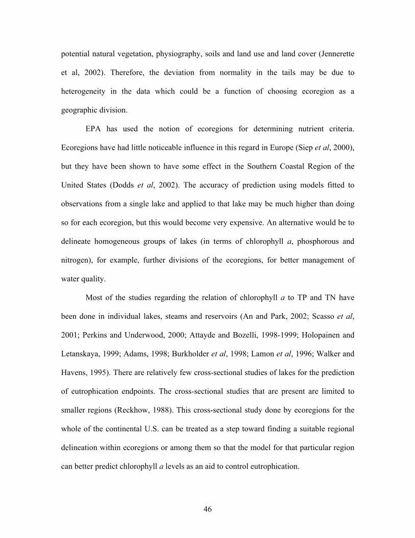
EPA has used the notion of ecoregions for determining nutrient criteria.
Ecoregions have had little noticeable influence in this regard in Europe (Siep et al, 2000),
but they have been shown to have some effect in the Southern Coastal Region of the
United States (Dodds et al, 2002). The accuracy of prediction using models fitted to
observations from a single lake and applied to that lake may be much higher than doing
so for each ecoregion, but this would become very expensive. An alternative would be to
delineate homogeneous groups of lakes (in terms of chlorophyll a, phosphorous and
nitrogen), for example, further divisions of the ecoregions, for better management of
water quality.
Most of the studies regarding the relation of chlorophyll a to TP and TN have
been done in individual lakes, steams and reservoirs (An and Park, 2002; Scasso et al,
2001; Perkins and Underwood, 2000; Attayde and Bozelli, 1998-1999; Holopainen and
Letanskaya, 1999; Adams, 1998; Burkholder et al, 1998; Lamon et al, 1996; Walker and
Havens, 1995). There are relatively few cross-sectional studies of lakes for the prediction
of eutrophication endpoints. The cross-sectional studies that are present are limited to
smaller regions (Reckhow, 1988). This cross-sectional study done by ecoregions for the
whole of the continental U.S. can be treated as a step toward finding a suitable regional
delineation within ecoregions or among them so that the model for that particular region
can better predict chlorophyll a levels as an aid to control eutrophication.
46

Of the 593,650 observations, the study used 93,894 observations. The ecoregions
did not have equal number of samples. The variability in the number of observations in
each ecoregion for each model ranged from 15 to more than 50,000 (Appendix C).
Therefore, the method of sample collection could be improved by making sure that all
observations are taken simultaneously, so that a larger dataset might be used for better
prediction.
Other Approaches
There are instances when models show a quadratic relation of chlorophyll a with
TP, with chlorophyll a reaching an asymptote at high TP. An and Park (2002) found that
using a quadratic model explained about 45% more of the variation in their data than a
linear relationship. Model 4, 5, and 6 in this study (Figures 14, 17 and 20) show some
non-linearity. So, this might be another approach for finding the best model to use for
prediction of chlorophyll a.
Another approach to dealing with non-linearity is a semiparametric model
(Lamon and Clyde, 2000). This model includes the explanatory variables (e.g., TP and
TN) as linear predictors or regression spline predictors, and this can account for nonlinear
relationships. Bayesian model averaging was used by Lamon and Clyde (2000) for
predictions that included uncertainty about inclusion of variables (model specifications).
The data in each ecoregion show great variation. Using breakpoint regression
could help to find two linear relationships that might describe the highest proportion of
variance in the ecoregion (Dodds et al, 2002). This could then be used to form smaller but
more homogeneous regions with respect to lake type.
47

In a linear regression, the parameters are assumed to be constant for all
observations. But in cross-sectional or time series data, the parameters might vary among
the cross-sectional units or over time. This problem might be solved by explicitly
modeling the unmodeled factors to make them predictable. But, there might be cases
where this modeling will not be feasible (data scarce, unavailable, etc.). In this case a
random coefficient regression model can be used where the parameter reflects the
variance over cross-sectional data (Reckhow, 1992).
Summary/Conclusion
Section 304 of the Clean Water Act deals with a scientific assessment of
ecological and human health effects recommended by EPA to the States and Tribes for
establishing water quality standards. These serve as a basis for control of discharges or
release of pollutants. The EPA has divided the continental United States into fourteen
ecoregions to facilitate the management of water quality. EPA intends to use this
scientific assessment to develop default Section 304(a) nutrient criteria for the all the
ecoregions in the country. They have identified nutrient measures (like total phosphorous,
soluble reactive phosphorus, total nitrogen, total Kjeldahl nitrogen, plant biomass and
land use) that can be used to formulate standards for water quality. According to EPA,
the main causal variables in establishing these standards are total phosphorous and total
nitrogen, and the indicator response variables are chlorophyll a and Secchi depth.
In the nutrient criteria database, sampling for phosphorous, nitrogen and
chlorophyll a have not been done following the same methods for the same variable. So,
all the samples cannot be used for all ecoregions to fit a linear model. A regression
analysis of several combinations of TP, nitrogen and chlorophyll a method types was
48

done to find the best combination that can be used in future studies to predict
eutrophication endpoints. It was found that model 5 is the best in terms of number of
observations, geographic coverage and model fit (R2) of chlorophyll a that can be
explained by TP and TKN.
Since lakes vary within ecoregions due to natural and anthropogenic factors, it
would be ideal to have a standard for each lake. But, it would be very expensive to collect
data and develop models to predict chlorophyll a for each individual lake. This is why
lakes should be grouped in a way so that a particular model for prediction of chlorophyll
a can be used for the all the lakes in the group. The ecoregion approach is a broad
approach. The differences in lakes within an ecoregion may not be well explained by the
differences used to create the ecoregions. An additional subdivision of lakes can be
accomplished (by conditioning on TP and TN) with these empirical models. Model 5 can
be used in further studies to find the best subdivision of ecoregions to set standards for
water quality.
There is evidence of non-linearity in models 4, 5, and 6 in this study between the
response and predictor variables (Figures 14, 17, and 20). Residuals from Model 5 were
plotted against logTKN (Figure 22). This shows a random scatter of points which
indicates an approximately random pattern. Residuals were plotted against logTP (Figure
23). This shows nonlinearity as indicated by the conical shape at the end. Nonlinear
quadratic relationships between chlorophyll a and TP and TN, semiparametric models,
breakpoint regression and a random coefficient regression model are some of the
alternatives to linear models.
49

log10[TKN]
residual
-1.5 -1.0 -0.5 0.0 0.5
-3-2
-10
1
Figure 22: LogTKN vs. residual plot for Model 5.
log10[TP]
residual
-2.5 -2.0 -1.5 -1.0 -0.5 0.0
-3-2
-10
1
Figure 23: LogTP vs. residual plot for Model 5.
From the models, it is seen that nutrients can explain some of the variance in
chlorophyll a. But many factors that affect chlorophyll a (light, flushing, zooplankton
50

51
grazing, etc.) cannot be controlled. This leaves nutrient management as the most probable
tool in controlling eutrophication in water bodies (Dodds et al, 2002). Data collection
methods should be improved. This could be done by analyzing all the samples for all the
variables of concern. Sampling methods should be uniform for individual variables.
This work can be treated as a first step to formulating an appropriate model for
the prediction of eutrophication endpoints. The limitations and uncertainties encountered
while doing this analysis are important for understanding the drawbacks/gaps that need to
be addressed for finding the best model that takes into account these limitations and
offers a more reliable and practical approach for prediction of these endpoints.

REFERENCES Adams BAV. 1998. Parameter Distributions for Uncertainty Propagation in Water Quality Modeling. Dissertation Abstracts International Part B: Science and Engineering. 59(4) [np]. Alberts EE, Schuman GE, Burnwell RE. 1978. Seasonal runoff losses of nitrogen and phosphorous from Missouri Valley loess watersheds. Journal of Environmental Quality.7: 203-208. Ambrose Jr. RB, Wool TA, Connolly JP. 1988. WASP4, A hydrodynamic and water quality model-Model theory, user’s manual, and programmer’s guide. Environmental Research Laboratory. USEPA. Athens, GA.
An Kwang-Guk, Park SS. 2002. Indirect influence of the summer monsoon on chlorophyll-total phosphorus models in reservoirs: a case study. Ecological Modelling. 152(2-3): 191-203. Attayde JL, Bozelli RL. 1998-1999. Environmental heterogeneity patterns and predictive models of chlorophyll a in a Brazilian coastal lagoon. Hydrobiologia. 390(1-3): 129-139. Brown LC, Barnwell Jr. TO. 1987. The enhanced stream water quality models QUAL2E and QUAL2E-UNCAS: Documentation and user manual. Environmental Research Laboratory. USEPA. Athens, GA. Burkholder JM, Larsen LM, Glasgow HB Jr., Mason KM, Gama P, Parsons JE. 1998. Influence of sediment and phosphorus loading on phytoplankton communities in an urban piedmont reservoir. Lake and Reservoir Management. 14(1): 110-121.
Carlson RE. 1977. A trophic state index for lakes. Limnology and Oceanography. 22:361-369. Dodds WK, Smith VH, Lohman K. 2002. Nitrogen and phosphorus relationships to benthic algal biomass in temperate streams. Canadian Journal of Fisheries and Aquatic Sciences. 59(5): 865-874. Hamilton LC. 1992. Regression with graphics. Duxbury Press, Belmont, California.
Heiskary SA, Walker WW Jr. 1988. Developing phosphorus criteria for Minnesota lakes. Lake Reservoir Management 4(1):1-10. Henderson-Sellers , Markland HR. 1987. Decaying Lakes: the Origins and Control of Cultural Eutropjication. John Wiley and Sons. New York, Chichester, Brisbane, Toronto.
52

Holopainen A-L, Letanskaya GI. 1999. Effects of nutrient load on species composition and productivity of phytoplankton in Lake Ladoga. Boreal Environment Research. 4(3): 215-227. Jennerette GD, Lee J, Waller DW, Carlson RE. 2002. Multivariate analysis of the ecoregion delineation for aquatic systems. Environmental Management. 29(1): 67-75. Jones JR, Knowlton MF, Kaiser MS. 1998. Effects of aggregation on chlorophyll-phosphorus relations in Missouri reservoirs. Lake and Reservoir Management. 14(1): 1-9. Lamon EC III. 1995. A regression model for the prediction of chlorophyll a in Lake Okeechobee, Florida. Lake and Reservoir Management. 11(4): 283-290. Lamon EC III, Clyde MA. 2000. Accounting for model uncertainty in prediction of chlorophyll a in Lake Okeechobee. Journal of Agricultural, Biological, and Environmental Statistics. 5(3): 297-322. Lamon EC III, Reckhow KH, Havens KE. 1996. Using generalized additive models for prediction of chlorophyll a in Lake Okeechobee, Florida. Lakes & Reservoirs: Research and Management. 2(1-2): 37-46. Laws EA. 1981. Aquatic Pollution. John Wiley and Sons. New York, Chichester, Brisbane, Toronto. Marlene NaaNes. Drought, algae levels take life from lake, give rotten odor. 06/03/03. Advocate (2theadvocate.com).
North American Lake Management Society. 1992. Developing eutrophication standards for lakes and reservoirs. Report prepared by the Lake Standards Subcommittee. Alachua, FL. 51 pp. Novotny V, Olem H.1994. Water Quality: Prevention, Identification and Management of diffuse pollution. Van Norstrand Reinhold, New York.
Omernik JM. 1987. Ecoregions of the conterminous United States. Annals. Association of American Geographers. 77(1):118-125.
Omernik JM. 1995. Ecoregions: A framework for managing ecosystems. George Wright Forum 12(1):35-50. Omernik JM, Larsen DP, Rohm CM, et al. 1988. Summer total phosphorus in lakes: A map of Minnesota, Wisconsin, and Michigan. Environmental Management. 12:815-825. Omernik JM. 2000. Draft Aggregations of Level III Ecoregions for the National Nutrient Strategy. [http://www.epa.gov/ost/standards/ecomap.htm]
53

Perkins RG, Underwood GJC. 2000. Gradients of chlorophyll a and water chemistry along an eutrophic reservoir with determination of the limiting nutrient by in situ nutrient addition. Water Research. 34(3): 713-724. Reckhow KH. 1988. Empirical models for trophic state in southeastern U. S. Lakes and reservoirs. 24(4): 723-734. Reckhow, KH. 1994. A decision analytic framework for environmental analysis and simulation modeling. Environmental Toxicology and Chemistry. 13(12): 1901-1906. Reckhow KH, Chapra SC. 1983. Engineering approaches for lake management, Volume 1. Butterworth Publishers. Reckhow KH, Coffey SC, Henning MH, Smith K, Banting R. 1992. EUTROMOD: Technical guidance and spreadsheet models for nutrient loading and lake eutrophication, North American Lake Management Society.
Reckhow KH, Simpson JT. 1980. A procedure using modeling and error analysis for the prediction of the lake phosphorus concentration from land use information. Canadian Journal of Fisheries and Aquatic Sciences. 37:1439-1448. Ryther JH, Dunstan WM. 1971. Nitrogen, phosphorous and eutrophication in the coastal marine environment. Science. 171: 1008-1013. Scasso F, Mazzeo N, Gorga J, Kruk C, Lacerot G, Clemente J, Fabian D, Bonilla S. 2001. Limnological changes in a sub-tropical shallow hypertrophic lake during its restoration: two years of a whole-lake experiment. Aquatic Conservation: Marine and Freshwater Ecosystems. 11(1): 31-44. Schindler DW. 1974. Eutrophication and recovery in experimental lakes: Implications in lake management. Science. 184: 897-899. Siep KL, Jeppsen E, Jensen JP, Faafeng B. 2000. Is trophic state or regional locationthe strongest determinant for Chl-a/TP relationships in lakes? Aquatic Sciences. 62(3): 195-204.
U.S. EPA 2002. Ambient Water Quality Criteria Recommendations Information Supporting the Development of State and Tribal Nutrient Criteria Lakes and Reservoirs in Nutrient Ecoregion I. U.S. Environmental Protection Agency, Washington, DC. EPA 822-R-02-050. U.S. EPA. 2000. Methodology for Deriving Ambient Water Quality Criteria for the Protection of Human Health. U.S. Environmental Protection Agency, Washington, DC. EPA-822-B-00-004.
54

55
U.S. EPA. 2000. National Water Quality Inventory, 2000 Report. U.S. Environmental Protection Agency, Washington, DC.
U.S. EPA. 2000a. Nutrient Criteria Technical Guidance Manual: Lakes and Reservoirs. U.S. Environmental Protection Agency, Washington, DC. EPA-822-B00-001. Van der Molen, DT, Portielje, R. 1999. Relationships between eutrophication variables: from nutrient loading to transparency. Hydrobiologia. 408/409: 359-365. Vollenweider, RA. 1969. Possibilities and limits of elementary models concerning the budget of substances in lakes. Archiv fuer Hydrobiologie. 66(1): 1-36. Walker, W.W. 1985a. Statistical bases for mean chlorophyll a criteria. pp. 57-62 In Lake and Reservoir Management: Practical Applications. Proceedings of the Fourth Annual Conference and International Symposium. October 16-19, 1984. North American Lake Management Society, McAfee, NJ. Walker WW Jr.1985b. Urban nonpoint source impacts on surface water supply. Perspectives on nonpoint source pollution. Proceedings of a national conference, Kansas City, MO, May 19-22, 1985, pp.129-137. U.S.Environmental Protection Agency. EPA 440/5-85-01. Walker WW Jr., Havens KE. 1995. Relating algal bloom frequencies to phosphorus concentrations in Lake Okeechobee. Lake and Reservoir Management. 11(1): 77-83.

APPENDIX A CONSENT FORM
56

Privacy and Security Notice
Recent Additions | Contact Us | Print Version Search: Advanced Search EPA Home > Privacy and Security Notice
About Privacy and Security
1. This World Wide Web (WWW) site is provided as a public service by the Environmental Protection Agency.
2. Information presented on this WWW site is considered public information and may be distributed or copied. The U.S. Government retains a nonexclusive, royalty-free license to publish or reproduce these documents, or allow others to do so, for U.S. Government purposes. These documents may be freely distributed and used for non-commercial, scientific and educational purposes. Commercial use of the documents available from this server may be protected under the U.S. and Foreign Copyright Laws. Individual documents on this server may have different copyright conditions, and that will be noted in those documents.
3. When you come to this web site to browse, you do so anonymously. EPA does not collect identifying information about you. We collect only summary information [see below] about the numbers of individuals who visit our web site and what those individuals look at. This government computer system uses industry-standard software to create summary statistics, which are used for such things as assessing what information is of most and least interest, determining technical design specifications, and identifying system performance or problem areas.
4. Where identifying information is asked of you (to respond to an information request, etc.) that information is used only for responding to your comment or question and is not made available for other purposes. See our comments notice of use.
5. For site security purposes and to ensure that this service remains available to all users, this government computer system employs industry-standard methods to monitor network traffic to identify unauthorized attempts to upload or change information, or otherwise cause damage.
6. No other attempts are made to identify individual users or their usage habits. Raw data logs are used for no other purposes and are scheduled for regular destruction in accordance with National Archives and Records Administration guidelines.
7. Unauthorized attempts to upload information or change information on this service are strictly prohibited and may be punishable under the Computer Fraud and Abuse Act of 1986.
If you have any questions or comments about the information presented here, please forward them to us through the address on our Comments Page.
57

58
EPA Home | Accessibility | Privacy and Security Notice | FOIA | Contact Us
This page was generated on Thursday, June 26, 2003
View the graphical version of this page at: http://www.epa.gov/epahome/usenotice.htm

APPENDIX B SAS ANOVA OUTPUT FOR MODELS
59

SAS Anova Output for Model 1 The SAS System The GLM Procedure Class Level Information Class Levels Values ECOREGION_ID 3 2 7 8 Number of observations 4246 Dependent Variable: logCHLA Sum of Source DF Squares Mean Square F Value Pr > F Model 9 1630.274856 181.141651 1727.06 <.0001 Error 4237 444.395785 0.104885 Uncorrected Total 4246 2074.670641 R-Square Coeff Var Root MSE logCHLA Mean 0.280531 55.28613 0.323859 0.585787 Source DF Type I SS Mean Square F Value Pr > F ECOREGION_ID 3 1543.387733 514.462578 4905.04 <.0001 logTP*ECOREGION_ID 3 83.146523 27.715508 264.25 <.0001 logTN*ECOREGION_ID 3 3.740600 1.246867 11.89 <.0001 Source DF Type III SS Mean Square F Value Pr > F ECOREGION_ID 3 242.4560533 80.8186844 770.55 <.0001 logTP*ECOREGION_ID 3 76.1004409 25.3668136 241.85 <.0001 logTN*ECOREGION_ID 3 3.7406003 1.2468668 11.89 <.0001 Standard Parameter Estimate Error t Value Pr > |t| ECOREGION_ID 2 1.231016797 0.04008926 30.71 <.0001 ECOREGION_ID 7 1.567993796 0.04959061 31.62 <.0001 ECOREGION_ID 8 2.160235259 0.11245924 19.21 <.0001 logTP*ECOREGION_ID 2 0.262851846 0.02570754 10.22 <.0001 logTP*ECOREGION_ID 7 0.479468690 0.02644438 18.13 <.0001 logTP*ECOREGION_ID 8 0.914703768 0.05350348 17.10 <.0001 logTN*ECOREGION_ID 2 0.048957431 0.03561909 1.37 0.1694 logTN*ECOREGION_ID 7 0.236321104 0.06124053 3.86 0.0001 logTN*ECOREGION_ID 8 -0.271911108 0.06257249 -4.35 <.0001
60

Tests for Normality Test --Statistic--- -----p Value------ Kolmogorov-Smirnov D 0.05365 Pr > D <0.0100 Cramer-von Mises W-Sq 2.820438 Pr > W-Sq <0.0050 Anderson-Darling A-Sq 18.43623 Pr > A-Sq <0.0050
SAS Anova Output for Model 2
The SAS System The GLM Procedure Class Level Information Class Levels Values ECOREGION_ID 7 1 11 14 2 7 8 9 Number of observations 5069 Dependent Variable: logCHLA Sum of Source DF Squares Mean Square F Value Pr > F Model 21 4015.644699 191.221176 787.73 <.0001 Error 5048 1225.397727 0.242749 Uncorrected Total 5069 5241.042426 R-Square Coeff Var Root MSE logCHLA Mean 0.230490 58.07333 0.492696 0.848403 Source DF Type I SS Mean Square F Value Pr > F ECOREGION_ID 7 3767.090731 538.155819 2216.92 <.0001 logTP*ECOREGION_ID 7 151.471102 21.638729 89.14 <.0001 logTKN*ECOREGION_ID 7 97.082865 13.868981 57.13 <.0001 Source DF Type III SS Mean Square F Value Pr > F ECOREGION_ID 7 778.6225599 111.2317943 458.22 <.0001 logTP*ECOREGION_ID 7 73.0806366 10.4400909 43.01 <.0001 logTKN*ECOREGION_ID 7 97.0828654 13.8689808 57.13 <.0001 Standard Parameter Estimate Error t Value Pr > |t| ECOREGION_ID 1 0.481217024 0.65419533 0.74 0.4620 ECOREGION_ID 11 0.738267367 0.11222459 6.58 <.0001 ECOREGION_ID 14 1.534680297 0.09550770 16.07 <.0001 ECOREGION_ID 2 0.351149711 0.31728827 1.11 0.2685
61

ECOREGION_ID 7 3.010657369 0.23784482 12.66 <.0001 ECOREGION_ID 8 0.777132461 0.50458496 1.54 0.1236 ECOREGION_ID 9 1.539826263 0.02940787 52.36 <.0001 logTP*ECOREGION_ID 1 -1.305012496 1.26180365 -1.03 0.3011 logTP*ECOREGION_ID 11 0.150387217 0.05946478 2.53 0.0115 logTP*ECOREGION_ID 14 0.336339249 0.05717160 5.88 <.0001 logTP*ECOREGION_ID 2 -0.684675591 0.27447634 -2.49 0.0126 logTP*ECOREGION_ID 7 1.235723281 0.12755220 9.69 <.0001 logTP*ECOREGION_ID 8 0.263698966 0.34106070 0.77 0.4395 logTP*ECOREGION_ID 9 0.257178131 0.02044047 12.58 <.0001 logTKN*ECOREGION_ID 1 1.891124394 1.10468920 1.71 0.0870 logTKN*ECOREGION_ID 11 0.101809423 0.06783917 1.50 0.1335 logTKN*ECOREGION_ID 14 0.300424208 0.07585771 3.96 <.0001 logTKN*ECOREGION_ID 2 1.555524362 0.24855602 6.26 <.0001 logTKN*ECOREGION_ID 7 0.168823228 0.17376405 0.97 0.3313 logTKN*ECOREGION_ID 8 -0.095241675 0.39095783 -0.24 0.8075 logTKN*ECOREGION_ID 9 0.559824049 0.03041020 18.41 <.0001 Tests for Normality Test --Statistic--- -----p Value------ Kolmogorov-Smirnov D 0.053683 Pr > D <0.0100 Cramer-von Mises W-Sq 5.598006 Pr > W-Sq <0.0050 Anderson-Darling A-Sq 35.26148 Pr > A-Sq <0.0050
SAS Anova Output for Model 3
The SAS System The GLM Procedure Class Level Information Class Levels Values ECOREGION_ID 4 11 2 7 8 Number of observations 4817 Dependent Variable: logCHLA Sum of Source DF Squares Mean Square F Value Pr > F Model 12 1803.492198 150.291017 1263.15 <.0001 Error 4805 571.705879 0.118981 Uncorrected Total 4817 2375.198078 R-Square Coeff Var Root MSE logCHLA Mean 0.274044 60.08236 0.344937 0.574107
62
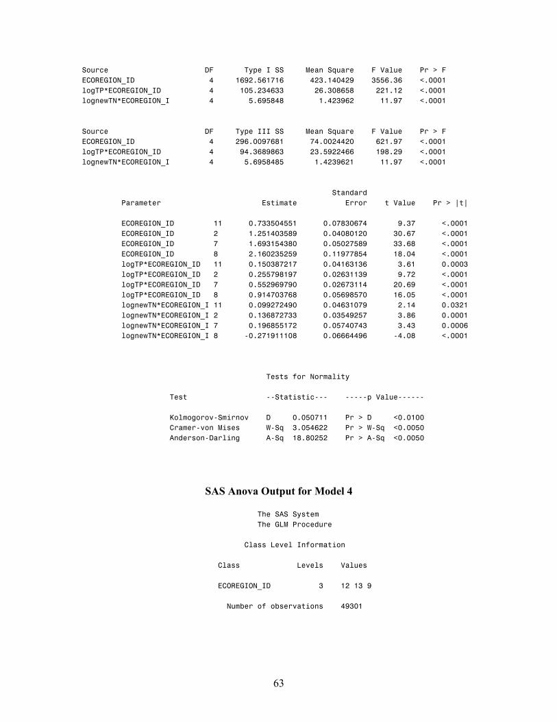
Source DF Type I SS Mean Square F Value Pr > F ECOREGION_ID 4 1692.561716 423.140429 3556.36 <.0001 logTP*ECOREGION_ID 4 105.234633 26.308658 221.12 <.0001 lognewTN*ECOREGION_I 4 5.695848 1.423962 11.97 <.0001 Source DF Type III SS Mean Square F Value Pr > F ECOREGION_ID 4 296.0097681 74.0024420 621.97 <.0001 logTP*ECOREGION_ID 4 94.3689863 23.5922466 198.29 <.0001 lognewTN*ECOREGION_I 4 5.6958485 1.4239621 11.97 <.0001 Standard Parameter Estimate Error t Value Pr > |t| ECOREGION_ID 11 0.733504551 0.07830674 9.37 <.0001 ECOREGION_ID 2 1.251403589 0.04080120 30.67 <.0001 ECOREGION_ID 7 1.693154380 0.05027589 33.68 <.0001 ECOREGION_ID 8 2.160235259 0.11977854 18.04 <.0001 logTP*ECOREGION_ID 11 0.150387217 0.04163136 3.61 0.0003 logTP*ECOREGION_ID 2 0.255798197 0.02631139 9.72 <.0001 logTP*ECOREGION_ID 7 0.552969790 0.02673114 20.69 <.0001 logTP*ECOREGION_ID 8 0.914703768 0.05698570 16.05 <.0001 lognewTN*ECOREGION_I 11 0.099272490 0.04631079 2.14 0.0321 lognewTN*ECOREGION_I 2 0.136872733 0.03549257 3.86 0.0001 lognewTN*ECOREGION_I 7 0.196855172 0.05740743 3.43 0.0006 lognewTN*ECOREGION_I 8 -0.271911108 0.06664496 -4.08 <.0001 Tests for Normality Test --Statistic--- -----p Value------ Kolmogorov-Smirnov D 0.050711 Pr > D <0.0100 Cramer-von Mises W-Sq 3.054622 Pr > W-Sq <0.0050 Anderson-Darling A-Sq 18.80252 Pr > A-Sq <0.0050
SAS Anova Output for Model 4
The SAS System The GLM Procedure Class Level Information Class Levels Values ECOREGION_ID 3 12 13 9 Number of observations 49301
63

Dependent Variable: logCHLAtri Sum of Source DF Squares Mean Square F Value Pr > F Model 9 54805.55345 6089.50594 53892.4 <.0001 Error 49292 5569.69428 0.11299 Uncorrected Total 49301 60375.24773 R-Square Coeff Var Root MSE logCHLAtri Mean 0.607496 34.72997 0.336146 0.967883 Source DF Type I SS Mean Square F Value Pr > F ECOREGION_ID 3 46290.92148 15430.30716 136559 <.0001 logTP*ECOREGION_ID 3 7674.39147 2558.13049 22639.5 <.0001 logTN*ECOREGION_ID 3 840.24050 280.08017 2478.72 <.0001 Source DF Type III SS Mean Square F Value Pr > F ECOREGION_ID 3 9200.368610 3066.789537 27141.2 <.0001 logTP*ECOREGION_ID 3 2011.978456 670.659485 5935.36 <.0001 logTN*ECOREGION_ID 3 840.240504 280.080168 2478.72 <.0001 Standard Parameter Estimate Error t Value Pr > |t| ECOREGION_ID 12 2.118677800 0.00760272 278.67 <.0001 ECOREGION_ID 13 1.887067346 0.04230991 44.60 <.0001 ECOREGION_ID 9 2.420275175 0.05744195 42.13 <.0001 logTP*ECOREGION_ID 12 0.621876411 0.00475086 130.90 <.0001 logTP*ECOREGION_ID 13 0.519484773 0.02692492 19.29 <.0001 logTP*ECOREGION_ID 9 0.725213006 0.04189370 17.31 <.0001 logTN*ECOREGION_ID 12 0.646263468 0.00757070 85.36 <.0001 logTN*ECOREGION_ID 13 0.428154791 0.08054478 5.32 <.0001 logTN*ECOREGION_ID 9 0.722803987 0.06572837 11.00 <.0001 Tests for Normality Test --Statistic--- -----p Value------ Kolmogorov-Smirnov D 0.034347 Pr > D <0.0100 Cramer-von Mises W-Sq 25.95156 Pr > W-Sq <0.0050 Anderson-Darling A-Sq 182.3509 Pr > A-Sq <0.0050
64

SAS Anova output for Model 5
The SAS System The GLM Procedure Class Level Information Class Levels Values ECOREGION_ID 10 10 11 12 13 2 3 6 7 8 9 Number of observations 20681 Dependent Variable: logCHLAtri Sum of Source DF Squares Mean Square F Value Pr > F Model 30 29724.35587 990.81186 7416.46 <.0001 Error 20651 2758.89717 0.13360 Uncorrected Total 20681 32483.25304 R-Square Coeff Var Root MSE logCHLAtri Mean 0.480209 31.88554 0.365508 1.146313 Source DF Type I SS Mean Square F Value Pr > F ECOREGION_ID 10 27611.61387 2761.16139 20667.9 <.0001 logTP*ECOREGION_ID 10 1714.46846 171.44685 1283.32 <.0001 logTKN*ECOREGION_ID 10 398.27353 39.82735 298.12 <.0001 Source DF Type III SS Mean Square F Value Pr > F ECOREGION_ID 10 3813.891338 381.389134 2854.79 <.0001 logTP*ECOREGION_ID 10 436.405816 43.640582 326.66 <.0001 logTKN*ECOREGION_ID 10 398.273534 39.827353 298.12 <.0001 Standard Parameter Estimate Error t Value Pr > |t| ECOREGION_ID 10 2.359215541 1.02278022 2.31 0.0211 ECOREGION_ID 11 1.475358834 0.06872305 21.47 <.0001 ECOREGION_ID 12 1.702749554 0.01477653 115.23 <.0001 ECOREGION_ID 13 1.690133009 0.02537298 66.61 <.0001 ECOREGION_ID 2 1.519924153 0.39809402 3.82 0.0001 ECOREGION_ID 3 1.320811280 0.21079561 6.27 <.0001 ECOREGION_ID 6 1.566600500 0.03556858 44.04 <.0001 ECOREGION_ID 7 1.811234703 0.02141959 84.56 <.0001 ECOREGION_ID 8 2.125527877 0.09069597 23.44 <.0001 ECOREGION_ID 9 1.276928827 0.04924022 25.93 <.0001 logTP*ECOREGION_ID 10 0.875672742 1.88953312 0.46 0.6431 logTP*ECOREGION_ID 11 0.447838758 0.03684421 12.15 <.0001 logTP*ECOREGION_ID 12 0.375003092 0.01017208 36.87 <.0001
65

logTP*ECOREGION_ID 13 0.389942366 0.01782133 21.88 <.0001 logTP*ECOREGION_ID 2 -0.118101064 0.30897569 -0.38 0.7023 logTP*ECOREGION_ID 3 -0.335845116 0.19374216 -1.73 0.0830 logTP*ECOREGION_ID 6 0.309564435 0.03107306 9.96 <.0001 logTP*ECOREGION_ID 7 0.490158208 0.01508020 32.50 <.0001 logTP*ECOREGION_ID 8 0.642072683 0.05818802 11.03 <.0001 logTP*ECOREGION_ID 9 -0.019048272 0.04879490 -0.39 0.6963 logTKN*ECOREGION_ID 10 0.907658007 1.89943249 0.48 0.6328 logTKN*ECOREGION_ID 11 0.199194495 0.02430038 8.20 <.0001 logTKN*ECOREGION_ID 12 0.838190888 0.01842419 45.49 <.0001 logTKN*ECOREGION_ID 13 0.679190700 0.05435111 12.50 <.0001 logTKN*ECOREGION_ID 2 1.697315158 0.37793557 4.49 <.0001 logTKN*ECOREGION_ID 3 1.785696140 0.25553549 6.99 <.0001 logTKN*ECOREGION_ID 6 0.005126539 0.04259061 0.12 0.9042 logTKN*ECOREGION_ID 7 0.672374552 0.02795946 24.05 <.0001 logTKN*ECOREGION_ID 8 0.133359767 0.07750587 1.72 0.0853 logTKN*ECOREGION_ID 9 0.512466542 0.08358376 6.13 <.0001 Tests for Normality Test --Statistic--- -----p Value------ Kolmogorov-Smirnov D 0.054246 Pr > D <0.0100 Cramer-von Mises W-Sq 24.14828 Pr > W-Sq <0.0050 Anderson-Darling A-Sq 146.2811 Pr > A-Sq <0.0050
SAS Anova Output for Model 6
The SAS System The GLM Procedure Class Level Information Class Levels Values ECOREGION_ID 6 11 12 13 2 7 9 Number of observations 62475 Dependent Variable: logCHLAtri Sum of Source DF Squares Mean Square F Value Pr > F Model 18 72353.65913 4019.64773 33353.4 <.0001 Error 62457 7527.11954 0.12052 Uncorrected Total 62475 79880.77867
66

67
R-Square Coeff Var Root MSE logCHLAtri Mean 0.583141 34.89782 0.347155 0.994776 Source DF Type I SS Mean Square F Value Pr > F ECOREGION_ID 6 62404.70893 10400.78482 86301.5 <.0001 logTP*ECOREGION_ID 6 8900.27050 1483.37842 12308.5 <.0001 lognewTN*ECOREGION_I 6 1048.67970 174.77995 1450.25 <.0001 Source DF Type III SS Mean Square F Value Pr > F ECOREGION_ID 6 11140.27599 1856.71266 15406.3 <.0001 logTP*ECOREGION_ID 6 2261.97477 376.99579 3128.16 <.0001 lognewTN*ECOREGION_I 6 1048.67970 174.77995 1450.25 <.0001 Standard Parameter Estimate Error t Value Pr > |t| ECOREGION_ID 11 1.466040179 0.06509604 22.52 <.0001 ECOREGION_ID 12 2.074289570 0.00743439 279.01 <.0001 ECOREGION_ID 13 1.680480508 0.02517821 66.74 <.0001 ECOREGION_ID 2 2.505844894 0.35647245 7.03 <.0001 ECOREGION_ID 7 1.810782528 0.02035535 88.96 <.0001 ECOREGION_ID 9 2.420275175 0.05932334 40.80 <.0001 logTP*ECOREGION_ID 11 0.447838758 0.03499419 12.80 <.0001 logTP*ECOREGION_ID 12 0.599469075 0.00464522 129.05 <.0001 logTP*ECOREGION_ID 13 0.382782137 0.01713821 22.34 <.0001 logTP*ECOREGION_ID 2 -0.118101064 0.29346137 -0.40 0.6874 logTP*ECOREGION_ID 7 0.490158208 0.01432299 34.22 <.0001 logTP*ECOREGION_ID 9 0.725213006 0.04326583 16.76 <.0001 lognewTN*ECOREGION_I 11 0.194230877 0.02250508 8.63 <.0001 lognewTN*ECOREGION_I 12 0.645501091 0.00734834 87.84 <.0001 lognewTN*ECOREGION_I 13 0.582397945 0.05034986 11.57 <.0001 lognewTN*ECOREGION_I 2 2.214693847 0.46837705 4.73 <.0001 lognewTN*ECOREGION_I 7 0.677888173 0.02677332 25.32 <.0001 lognewTN*ECOREGION_I 9 0.722803987 0.06788116 10.65 <.0001 Tests for Normality Test --Statistic--- -----p Value------ Kolmogorov-Smirnov D 0.036567 Pr > D <0.0100 Cramer-von Mises W-Sq 36.65631 Pr > W-Sq <0.0050 Anderson-Darling A-Sq 251.3934 Pr > A-Sq <0.0050

APPENDIX C TABLES WITH PARAMETER VALUES FOR EACH MODEL
68

Model 1: logCHLA = logTP + logTN
logCHLA β0 (Std. error)
β1 logTP (Std. error)
β 2 logTN (Std. error)
Ecoregion 2 1.2310 (0.0400)
0.2628 (0.0257)
0.0489 (0.0356)
7 1.5679 (0.0495)
0.4794 (0.0264)
0.2363 (0.0612)
8 2.1602 (0.1124)
0.9147 (0.0535)
-0.2719 (0.0625)
Model 2: logCHLA = logTP + logTKN
logCHLA β 0 (Std. error)
β 1 logTP
(Std. error)
β 2 logTKN
(Std. error) Ecoregion 1 0.4812
(0.6541) -1.3050 (1.2618)
1.8911 (1.1046)
2 0.3511 (0.3172)
-0.6846 (0.2744)
1.5555 (0.2485)
7 3.0106 (0.2378)
.2357 (0.1275)
0.1688 (0.1737)
8 0.7771 (0.5045)
0.2636 (0.3410)
-0.0952 (0.3909)
9 1.5398 (0.0294)
0.2571 (0.0204)
0.5598 (0.0304)
11 0.7382 (0.1122)
0.1503 (0.0594)
0.1018 (0.0678)
14 1.5346 (0.0955)
0.3363 (0.0571)
0.3004 (0.0758)
69

Model 3: logCHLA = logTP + lognewTN
logCHLA β 0 (Std. error)
β 1 logTP
(Std. error)
β 2 lognewTKN (Std. error)
Ecoregion 2 1.2514 (0.0408)
0.2557 (0.0263)
0.1368 (0.0354)
7 1.6931 (0.0502)
0.5529 (0.0267)
0.1968 (0.0574)
8 2.1602 (0.1197)
0.9147 (0.0569)
-0.2719 (0.0666)
11 0.7335 (0.0783)
0.1503 (0.0416)
0.0992 (0.0463)
Model 4: logCHLAtri = logTP + logTN
logCHLAtri β 0 (Std. error)
β 1 logTP
(Std. error)
β 2 logTN
(Std. error) Ecoregion 9 2.4202
(0.0574) 0.7252
(0.0418) 0.7228
(0.0657) 12 2.1186
(0.0076) 0.6218
(0.0047) 0.6462
(0.0075) 13 1.8870
(0.0423) 0.5194
(0.0269) 0.4281
(0.0805)
70

Model 5: logCHLAtri = logTP + logTKN
logCHLAtri β 0 (Std. error)
β 1 logTP
(Std. error)
β 2 logTKN
(Std. error) Ecoregion 2 1.5199
(0.3980) -0.1181 (0.3089)
1.6973 (0.3779)
3 1.3208 (0.2107)
-0.3358 (0.1937)
1.7856 (0.2555)
6 1.5666 (0.0355)
0.3095 (0.0310)
0.0051 (0.0425)
7 1.8112 (0.0214)
0.4901 (0.0150)
0.6723 (0.0279)
8 2.1255 (0.0906)
0.6420 (0.0581)
0.1333 (0.0775)
9 1.2769 (0.0492)
-0.0190 (0.0487)
0.5124 (0.0835)
10 2.3592 (1.0227)
0.8756 (1.8895)
0.9076 (1.8994)
11 1.4753 (0.0687)
0.4478 (0.0368)
0.1991 (0.0243)
12 1.7027 (0.0147)
0.3750 (0.0101)
0.8381 (0.0184)
13 1.6901 (0.0253)
0.3899 (0.0178)
0.6791 (0.0543)
Model 6: logCHLAtri = logTP + lognewTN
logCHLAtri β 0 (Std. error)
β 1 logTP
(Std. error)
β 2 lognewTN (Std. error)
Ecoregion 2 2.5058 (0.3564)
-0.1181 (0.2934)
2.2146 (0.4683)
7 1.8107 (0.0203)
0.4901 (0.0143)
0.6778 (0.0267)
9 2.4202 (0.0593)
0.7252 (0.0432)
0.7228 (0.0678)
11 1.4660 (0.0650)
0.4478 (0.0349)
0.1942 (0.0225)
12 2.0742 (0.0074)
0.5994 (0.0046)
0.6455 (0.0073)
13 1.6804 (0.0251)
0.3827 (0.0171)
0.5823 (0.0503)
71

Table: Number of data in each model by ecoregion. Model Eco1 Eco2 Eco3 Eco4 Eco5 Eco6 Eco7 Eco8 Eco9 Eco10 Eco11 Eco12 Eco13 Eco14
1 0 0 0 0 716 0 3045 485 0 0 0 0 0 00 1 3887 0 394 0 0 538
3 0 0 0 0 776 0 3162 485 0 0 394 0 0 00 1423 0 0 46349 1529 0
5 0 16 37 0 0 642 5525 597 231 7 899 8934 3793 00 5525 0 1423 0 899 50797 3815 0
2 15 60 0 0 0 17 58
4 0 0 0 0 0 0 0
6 0 16 0 0 0
72

APPENDIX D
BOXPLOTS OF DISTRIBUTION OF CHLOROPHYLL A FOR EACH MODEL BY ECOREGION
73

-10
12
2 7 8
Ecoregion
log1
0[C
HLA
]
MODEL 1 Log CHLABy Ecoregion
-0.5
0.0
0.5
1.0
1.5
2.0
1 2 7 8 9 11 14
Ecoregion
log1
0[C
HLA
]
MODEL 2 Log CHLABy Ecoregion
74

-10
12
2 7 8 11
Ecoregion
log1
0[C
HLA
]MODEL 3 Log CHLA
By Ecoregion
-1.0
-0.5
0.0
0.5
1.0
1.5
2.0
9 12 13
Ecoregion
log1
0[C
HLA
tri]
MODEL 4 Log CHLAtriBy Ecoregion
75

-2-1
01
2
2 3 6 7 8 9 10 11 12 13
Ecoregion
log1
0[C
HLA
tri]
MODEL 5 Log CHLAtriBy Ecoregion
-2-1
01
2
2 7 9 11 12 13
Ecoregion
log1
0[C
HLA
tri]
MODEL 6 Log CHLAtriBy Ecoregion
76

APPENDIX E MAPS OF THE SPATIAL DISTRIBUTION OF OBSERVATIONS FOR EACH
MODEL
77

USEPA Nutrient Criteria DatabaseModel 1
Figure : Spatial distributions of observations for Model 1
78

USEPA Nutrient Criteria DatabaseModel 2
Figure : Spatial distributions of observations for Model 2
79

USEPA Nutrient Criteria DatabaseModel 3
Figure : Spatial distributions of observations for Model 3.
80

USEPA Nutrient Criteria DatabaseModel 4
Figure : Spatial distributions of observations for Model 4.
81

USEPA Nutrient Criteria DatabaseModel 5
Figure : Spatial distributions of observations for Model 5.
82

USEPA Nutrient Criteria DatabaseModel 6
83
Figure : Spatial distributions of observations for Model 6.

APPENDIX F SAS CODES
84

Arrangement in record format (example for Alabama): Data TP; set epalakes.lakeAL; if STORET_CODE=665; TP=REPORTED_VALUE; keep WATERBODY_ID_ WATERBODY_TYPE_ID STATION_ID STATE COUNTY ECOREGION_ID EPA_ECOREGION_ID SAMPLE_ID AGENCY_NAME SAMPLING_DATE SAMPLE_DEPTH LATITUDE LONGITUDE HYDROLOGIC_UNIT_CODE TP; run; proc sort; by STATION_ID SAMPLING_DATE SAMPLE_ID; run; data NO2; set epalakes.lakeAL; if STORET_CODE=615; NO2=REPORTED_VALUE; keep WATERBODY_ID_ WATERBODY_TYPE_ID STATION_ID STATE COUNTY ECOREGION_ID EPA_ECOREGION_ID SAMPLE_ID AGENCY_NAME SAMPLING_DATE SAMPLE_DEPTH LATITUDE LONGITUDE HYDROLOGIC_UNIT_CODE NO2; run; proc sort; by STATION_ID SAMPLING_DATE SAMPLE_ID; run; data DO; set epalakes.lakeAL; if STORET_CODE=300; DO=REPORTED_VALUE; keep WATERBODY_ID_ WATERBODY_TYPE_ID STATION_ID STATE COUNTY ECOREGION_ID EPA_ECOREGION_ID SAMPLE_ID AGENCY_NAME SAMPLING_DATE SAMPLE_DEPTH LATITUDE LONGITUDE HYDROLOGIC_UNIT_CODE DO; run; proc sort; by STATION_ID SAMPLING_DATE SAMPLE_ID; run; data TKN; set epalakes.lakeAL; if STORET_CODE=625; TKN=REPORTED_VALUE;
85

keep WATERBODY_ID_ WATERBODY_TYPE_ID STATION_ID STATE COUNTY ECOREGION_ID EPA_ECOREGION_ID SAMPLE_ID AGENCY_NAME SAMPLING_DATE SAMPLE_DEPTH LATITUDE LONGITUDE HYDROLOGIC_UNIT_CODE TKN; run; proc sort; by STATION_ID SAMPLING_DATE SAMPLE_ID; run; data NH3; set epalakes.lakeAL; if STORET_CODE=610; NH3=REPORTED_VALUE; keep WATERBODY_ID_ WATERBODY_TYPE_ID STATION_ID STATE COUNTY ECOREGION_ID EPA_ECOREGION_ID SAMPLE_ID AGENCY_NAME SAMPLING_DATE SAMPLE_DEPTH LATITUDE LONGITUDE HYDROLOGIC_UNIT_CODE NH3; run; proc sort; by STATION_ID SAMPLING_DATE SAMPLE_ID; run; data NO2NO3; set epalakes.lakeAL; if STORET_CODE=630; NO2NO3=REPORTED_VALUE; if STORET_CODE=10 then TEMP=REPORTED_VALUE; keep WATERBODY_ID_ WATERBODY_TYPE_ID STATION_ID STATE COUNTY ECOREGION_ID EPA_ECOREGION_ID SAMPLE_ID AGENCY_NAME SAMPLING_DATE SAMPLE_DEPTH LATITUDE LONGITUDE HYDROLOGIC_UNIT_CODE NO2NO3; run; proc sort; by STATION_ID SAMPLING_DATE SAMPLE_ID; run; data TEMP; set epalakes.lakeAL; if STORET_CODE=10; TEMP=REPORTED_VALUE; keep WATERBODY_ID_ WATERBODY_TYPE_ID STATION_ID STATE COUNTY ECOREGION_ID EPA_ECOREGION_ID SAMPLE_ID AGENCY_NAME SAMPLING_DATE SAMPLE_DEPTH LATITUDE LONGITUDE HYDROLOGIC_UNIT_CODE TEMP; run;
86

proc sort; by STATION_ID SAMPLING_DATE SAMPLE_ID; run; data epalakes.lakeAL; merge TP NO2 DO TKN NH3 NO2NO3 TEMP; by STATION_ID SAMPLING_DATE SAMPLE_ID; run; proc means; run; Merging datasets of all the states to form one dataset: data epalakes.lakeall; merge epalakes.lakeAL epalakes.lakeAR epalakes.lakeAZ epalakes.lakeCA epalakes.lakeCO epalakes.lakeCT epalakes.lakeDC epalakes.lakeDE epalakes.lakeGA epalakes.lakeIA epalakes.lakeID epalakes.lakeIL epalakes.lakeIN epalakes.lakeFL epalakes.lakeKS epalakes.lakeKY epalakes.lakeLA epalakes.lakeMA epalakes.lakeMD epalakes.lakeME epalakes.lakeMI epalakes.lakeMN epalakes.lakeMO epalakes.lakeMS epalakes.lakeMT epalakes.lakeNC epalakes.lakeND epalakes.lakeNE epalakes.lakeNH epalakes.lakeNJ epalakes.lakeNM epalakes.lakeNV epalakes.lakeNY epalakes.lakeOH epalakes.lakeOK epalakes.lakeOR epalakes.lakePA epalakes.lakeRI epalakes.lakeSC epalakes.lakeSD epalakes.lakeTN epalakes.lakeTX epalakes.lakeUT epalakes.lakeVA epalakes.lakeVT epalakes.lakeWA epalakes.lakeWI epalakes.lakeWV epalakes.lakeWY; by STATION_ID SAMPLING_DATE SAMPLE_ID; run; proc means; run; Regression of TN with TKN: data epalakes.TN_TKN ; /*making data set with TN TKN */ set epalakes.lakeall ; if TN ne . and TKN ne . ; run data TN_TKN ; set epalakes.TN_TKN ; logCHLAtri = log10(CHLAtri); logTP = log10(TP); logTN = log10(TN); logTKN = log10(TKN); run; proc sort data= TN_TKN ; by ecoregion_id ;
87

run proc means data = TN_TKN ; by ecoregion_id ; var TP TN TKN CHLAtri logTN logCHLAtri logTKN; run proc glm data= TN_TKN ; /* general linear model*/ class ecoregion_id ; model logTN = ecoregion_id ecoregion_id*logTKN / noint solution ; /* add these one by one to see if total number of samples vary because SAS will take only those data that have all non-missing values . Take either TN or TKN but not together */ id sampling_date ecoregion_id; output out= TN_TKN predicted=pred residual=res rstudent=jackres /* jack knife residual */ press=press h=h /* hat matrix*/ cookd=cookd ; /* cook's distance*/ run; Example of code for formation of variable “newTN”: libname epalakes "C:\Program Files\Insightful\splus6netclient\users"; data eco2; set epalakes.lakeall; if ecoregion_id = 2; logTN = log10(TN); logTKN = log10(TKN); pTN2=0; logTN2 = -0.445172475 + 0.766388167*(logTKN) ; if logTKN ne . then pTN2 = 1; TN2=10**(logTN2); /*(** = raise to the power of)*/ If TN ne . then newTN = TN; if TN = . then newTN = TN2; /* creating variable 'newTN' to include TN and predicted TN to get more observations*/ run; proc sort; by pTN2; run; proc means; by pTN2; var TN logTN TKN logTKN TN2 logTN2 pTN2 newTN ; run; proc means; var TN logTN TKN logTKN TN2 logTN2 pTN2 newTN ; run;
88

proc gplot; plot TN*TN2; run; Regression codes for each model: libname epalakes "C:\Program Files\Insightful\splus6netclient\users"; data CHLATPTN; /* Checking model 1 logCHLA = logTP + logTN*/ set epalakes.lakeall; logCHLA = log10(CHLA); logTP = log10(TP); logTN = log10(TN); if logCHLA ne . ; if logTP ne . ; if logTN ne . ; run; proc sort data= CHLATPTN ; by ecoregion_id ; run; proc means data = CHLATPTN ; by ecoregion_id ; var TP logTP TN logTN CHLA logCHLA ; run; proc glm data= CHLATPTN ; /* general linear model*/ class ecoregion_id ; model logCHLA = ecoregion_id ecoregion_id*logTP ecoregion_id*logTN / noint solution ; /* add these one by one to see if total number of samples vary because SAS will take only those data that have all non-missing values . Take either TN or TKN but not together */ id sampling_date ecoregion_id; output out= CHLATPTN predicted=pred residual=res rstudent=jackres /* jack knife residual */ press=press h=h /* hat matrix*/ cookd=cookd /* cook's distance*/ student = student ; run; proc univariate data = CHLATPTN normal plot ; var jackres student; run; libname epalakes "C:\Program Files\Insightful\splus6netclient\users"; data CHLATPTKN; /* checking model 2 logCHLA = logTP + logTKN */
89

set epalakes.lakeall; logCHLA = log10(CHLA); logTP = log10(TP); logTKN = log10(TKN); if logCHLA ne . ; if logTP ne . ; if logTKN ne . ; run; proc sort data= CHLATPTKN ; by ecoregion_id ; run; proc means data = CHLATPTKN ; by ecoregion_id ; var TP logTP TKN logTKN CHLA logCHLA ; run; proc glm data= CHLATPTKN ; /* general linear model*/ class ecoregion_id ; model logCHLA = ecoregion_id ecoregion_id*logTP ecoregion_id*logTKN / noint solution ; /* add these one by one to see if if total number of samples vary because SAS will take only those data that have all non-missing values . take either TN or TKN but not together */ id sampling_date ecoregion_id; output out= CHLATPTKN predicted=pred residual=res rstudent=jackres /* jack knife residual */ press=press h=h /* hat matrix*/ cookd=cookd /* cook's distance*/ student = student ; run; proc univariate data = CHLATPTKN normal plot ; var jackres student; run; libname epalakes "C:\Program Files\Insightful\splus6netclient\users"; data CHLATPnewTN; /*checking model 3 logCHLA = logTP + lognewTN . (do this for ecoregions 2,7,11,12,13 with respective formulae)*/ set epalakes.lakeall; logCHLA = log10(CHLA); logTP = log10(TP); logTKN = log10(TKN);
90
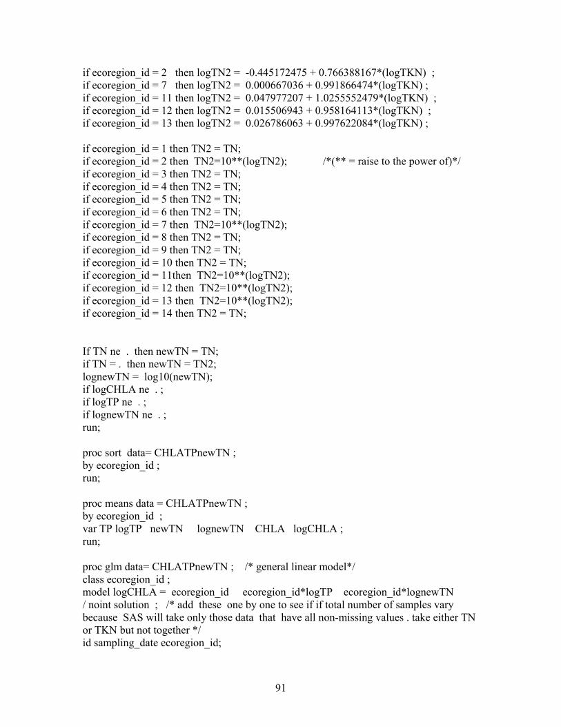
if ecoregion_id = 2 then logTN2 = -0.445172475 + 0.766388167*(logTKN) ; if ecoregion_id = 7 then logTN2 = 0.000667036 + 0.991866474*(logTKN) ; if ecoregion_id = 11 then logTN2 = 0.047977207 + 1.0255552479*(logTKN) ; if ecoregion_id = 12 then logTN2 = 0.015506943 + 0.958164113*(logTKN) ; if ecoregion_id = 13 then logTN2 = 0.026786063 + 0.997622084*(logTKN) ; if ecoregion_id = 1 then TN2 = TN; if ecoregion_id = 2 then TN2=10**(logTN2); /*(** = raise to the power of)*/ if ecoregion_id = 3 then TN2 = TN; if ecoregion_id = 4 then TN2 = TN; if ecoregion_id = 5 then TN2 = TN; if ecoregion_id = 6 then TN2 = TN; if ecoregion_id = 7 then TN2=10**(logTN2); if ecoregion_id = 8 then TN2 = TN; if ecoregion_id = 9 then TN2 = TN; if ecoregion_id = 10 then TN2 = TN; if ecoregion_id = 11then TN2=10**(logTN2); if ecoregion_id = 12 then TN2=10**(logTN2); if ecoregion_id = 13 then TN2=10**(logTN2); if ecoregion_id = 14 then TN2 = TN; If TN ne . then newTN = TN; if TN = . then newTN = TN2; lognewTN = log10(newTN); if logCHLA ne . ; if logTP ne . ; if lognewTN ne . ; run; proc sort data= CHLATPnewTN ; by ecoregion_id ; run; proc means data = CHLATPnewTN ; by ecoregion_id ; var TP logTP newTN lognewTN CHLA logCHLA ; run; proc glm data= CHLATPnewTN ; /* general linear model*/ class ecoregion_id ; model logCHLA = ecoregion_id ecoregion_id*logTP ecoregion_id*lognewTN / noint solution ; /* add these one by one to see if if total number of samples vary because SAS will take only those data that have all non-missing values . take either TN or TKN but not together */ id sampling_date ecoregion_id;
91

output out= CHLATPnewTN predicted=pred residual=res rstudent=jackres /* jack knife residual */ press=press h=h /* hat matrix*/ cookd=cookd /* cook's distance*/ student = student ; run; proc univariate data = CHLATPnewTN normal plot ; var jackres student; run; libname epalakes "C:\Program Files\Insightful\splus6netclient\users"; data CHLAtriTPTN; /* checking model 4 logCHLAtri = logTP + logTN*/ set epalakes.lakeall; logCHLAtri = log10(CHLAtri); logTP = log10(TP); logTN = log10(TN); if logCHLAtri ne . ; if logTP ne . ; if logTN ne . ; run; proc sort data= CHLAtriTPTN ; by ecoregion_id ; run; proc means data = CHLAtriTPTN ; by ecoregion_id ; var TP logTP TN logTN CHLAtri logCHLAtri ; run; proc glm data= CHLAtriTPTN ; /* general linear model*/ class ecoregion_id ; model logCHLAtri = ecoregion_id ecoregion_id*logTP ecoregion_id*logTN / noint solution ; /* add these one by one to see if if total number of samples vary because SAS will take only those data that have all non-missing values . take either TN or TKN but not together */ id sampling_date ecoregion_id; output out= CHLAtriTPTN predicted=pred residual=res rstudent=jackres /* jack knife residual */ press=press h=h /* hat matrix*/
92

cookd=cookd /* cook's distance*/ student = student ; run; proc univariate data = CHLAtriTPTN normal plot; /*gives univariate with plots and tests for normality for variables in the var statement*/ var jackres student; run; libname epalakes "C:\Program Files\Insightful\splus6netclient\users"; data CHLAtriTPTKN ; /*checking Model 5 : logCHLAtri = logTP + logTKN*/ set epalakes.lakeall ; logCHLAtri = log10(CHLAtri); logTP = log10(TP); logTKN = log10(TKN); if logCHLAtri ne . ; if logTP ne . ; if logTKN ne . ; run; proc sort data= CHLAtriTPTKN ; by ecoregion_id ; run; proc means data = CHLAtriTPTKN ; by ecoregion_id ; var TP logTP TKN logTKN CHLAtri logCHLAtri ; run; proc glm data= CHLAtriTPTKN ; /* general linear model*/ class ecoregion_id ; model logCHLAtri = ecoregion_id ecoregion_id*logTP ecoregion_id*logTKN / noint solution ; /* add these one by one to see if if total number of samples vary because SAS will take only those data that have all non-missing values . take either TN or TKN but not together */ id sampling_date ecoregion_id; output out= CHLAtriTPTKN predicted=pred residual=res rstudent=jackres /* jack knife residual */ press=press h=h /* hat matrix*/ cookd=cookd /* cook's distance*/ student = student ; run;
93

proc univariate data = CHLAtriTPTKN normal plot ; var jackres student; run; libname epalakes "C:\Program Files\Insightful\splus6netclient\users"; data CHLAtriTPnewTN; /*checking model 6 logCHLAtri = logTP + lognewTN . (do this for ecoregions 2,7,11,12,13 with respective formulae)*/ set epalakes.lakeall; logCHLAtri = log10(CHLAtri); logTP = log10(TP); logTKN = log10(TKN); if ecoregion_id = 2 then logTN2 = -0.445172475 + 0.766388167*(logTKN) ; if ecoregion_id = 7 then logTN2 = 0.000667036 + 0.991866474*(logTKN) ; if ecoregion_id = 11 then logTN2 = 0.047977207 + 1.0255552479*(logTKN) ; if ecoregion_id = 12 then logTN2 = 0.015506943 + 0.958164113*(logTKN) ; if ecoregion_id = 13 then logTN2 = 0.026786063 + 0.997622084*(logTKN) ; if ecoregion_id = 1 then TN2 = TN; if ecoregion_id = 2 then TN2=10**(logTN2); /*(** = raise to the power of)*/ if ecoregion_id = 3 then TN2 = TN; if ecoregion_id = 4 then TN2 = TN; if ecoregion_id = 5 then TN2 = TN; if ecoregion_id = 6 then TN2 = TN; if ecoregion_id = 7 then TN2=10**(logTN2); if ecoregion_id = 8 then TN2 = TN; if ecoregion_id = 9 then TN2 = TN; if ecoregion_id = 10 then TN2 = TN; if ecoregion_id = 11then TN2=10**(logTN2); if ecoregion_id = 12 then TN2=10**(logTN2); if ecoregion_id = 13 then TN2=10**(logTN2); if ecoregion_id = 14 then TN2 = TN; If TN ne . then newTN = TN; if TN = . then newTN = TN2; lognewTN = log10(newTN); if logCHLAtri ne . ; if logTP ne . ; if lognewTN ne . ; run; proc sort data= CHLAtriTPnewTN ; by ecoregion_id ; run; proc means data = CHLAtriTPnewTN ;
94

95
by ecoregion_id ; var TP logTP newTN lognewTN CHLAtri logCHLAtri ; run; proc glm data= CHLAtriTPnewTN ; /* general linear model*/ class ecoregion_id ; model logCHLAtri = ecoregion_id ecoregion_id*logTP ecoregion_id*lognewTN / noint solution ; /* add these one by one to see if if total number of samples vary because SAS will take only those data that have all non-missing values . Take either TN or TKN but not together */ id sampling_date ecoregion_id; output out= CHLAtriTPnewTN predicted=pred residual=res rstudent=jackres /* jack knife residual */ press=press h=h /* hat matrix*/ cookd=cookd /* cook's distance*/ student = student ; run; proc univariate data = CHLAtriTPnewTN normal plot ; var jackres student; run;

APPENDIX G SUMMARY STATISTICS FOR ECOREGIONS
96

Storet Codes and abbreviations Codes Parameter Abbreviation 10 Temperature (C) TEMP 11 Temperatrure (F) TF 60 Mean Daily Stream Flow, cfs MDS 61 Instantaneous Streamflow, cfs ISF 70 Turbidity JCU 76 Turbidity FTU 77 Secchi (inches) SECCHIin 78 Secchi (metres) SECCHI 94 Conductivity Field, ys/cm CF 95 Conductivity COND 300 Dissolved Oxygen, mg/l DO 301 Dissolved Oxygen (DO % saturated) DOsat 400 pH whole water field pH 403 pH whole water lab S.U. pHSU 409 Alkalinity, ueq/l ALKueq 410 Alkalinity Total (as CACO3) Field ALK 415 Alkalinity, Phenplphthalein, mg/l ALKP 500 Total Solids, mg/l TS 530 Residual Total Nonfiltrable, mg/l RTN 600 Nitrogen Total, mg/l TN 605 N_org total TON 608 Ammonia dissolved at 180 deg. mg/l as N NH3D 610 Ammonia Nitrogen Total NH3 615 Nitrate NO2 618 Nitrate dissolved as N, mg/l ND 620 Nitrate mg/l NO3 623 Nitrogen Kjeldhal dissolved as N, mg/l NKD 625 Nitrogen Total Kjeldhal, mg/l TKN 630 Nitrite and Nitrate, mg/l NO2NO3 631 Nitrite and Nitrate dissolved mg/l as N NND 660 Orthophosphate (OPO4_PO4), mg/l OPO4 665 Phosphorous Total, ug/l TP 666 Phosphorous Dissolved DP 669 Phosphorous Total Reactive, mg/l PTR 671 Orthophosphate dissolved mg/l as P OPD 915 Alkalinity, mg/l ALKmg 955 Silica dissolved, mg/l SIL 32209 Chlorophyll a Fluorometric corrected, ug/l CHLA 32210 Chlorophyll a Trichomatic uncorrected, ug/l CHLAtri 32211 Chlorophyll a Phytoplankton Spctophotometric Acid, ug/l CHLAphyt 32230 Chlorophyll a Phytoplankton spectrophotometric CHLAspec uncorrected, ug/l 49701 Secchi Disk Water Unfiltered, feet SDunfil
97

70300 Dissolved Solids (residue on evaporation *180C) DSE 70301 Dissolved Solids (sum of constituents), mg/l DS 70331 Sediment suspended percent finer than 0.062 mm FSS sieve diameter 70507 Phosphorous Orthophosphate Total POT 80154 Total suspended solid sediment suspended, mg/l TSS 82078 Turbidity (field) TURBf 82079 Turbidity (lab) TURBlab
98

The MEANS Procedure (For complete dataset ‘lakeall’) Variable Label N Mean Std Dev Minimum Maximum ƒƒƒƒƒƒƒƒƒƒƒƒƒƒƒƒƒƒƒƒƒƒƒƒƒƒƒƒƒƒƒƒƒƒƒƒƒƒƒƒƒƒƒƒƒƒƒƒƒƒƒƒƒƒƒƒƒƒƒƒƒƒƒƒƒƒƒƒƒƒƒƒƒƒƒƒƒƒƒƒƒƒƒƒƒƒƒƒƒƒƒƒƒƒƒƒƒƒ SAMPLING_DATE SAMPLING_DATE 593648 994143939 172722244 -234057600 1256083200 TP 324325 0.0787600 2.6520443 0 1486.00 NO2 20826 0.0088409 0.0185637 0 0.3300000 DO 123774 7.7206583 28.5233095 0 7400.00 TKN 91400 0.9422286 0.7932359 0 22.5000000 NH3 67622 0.1222654 0.2336343 0 4.4000000 NO2NO3 78850 0.4270715 2.6124017 -0.0600000 650.0000000 TEMP 214641 20.0803541 47.0852804 0 17000.00 NO3 82970 3.3681708 534.4894018 -0.0100000 88888.00 TURBIDITY 55597 7.6195082 14.4223530 0 1340.00 TURBf 3706 13.9358770 22.6166462 0.0800000 191.3000000 CHLAtri 79572 20.9721048 27.2996871 0 160.5500000 SECCHI 225988 3.3124659 2.2534222 0 23.0000000 SECCHIin 90275 55.8356245 45.9237217 1.0000000 288.0000000 TURBLAB 11500 14.2437383 19.9257704 0 197.0000000 TF 400 56.6540000 14.1786537 32.0000000 80.0000000 CHLAphyt 33416 21.7680154 28.1039865 0 254.5200000 TON 72277 2.7928538 331.0344305 -0.0600000 88888.00 TN 163838 2.2106112 311.7374630 -9999.00 88889.00 CHLA 15816 10.8619028 17.5862503 0 607.0000000 COND 79102 561.7922998 2967.21 -10.0000000 318000.00 pH 106994 8.8843761 385.0091860 0.2100000 88888.00 ALKueq 129 230.0375194 324.3410432 -51.8000000 1897.53 CHLAspec 24265 6.8579485 12.0245549 0 247.0000000 TSS 34147 18.6041170 503.6363311 -12.0000000 88888.00 ALKmg 34868 59.7922105 958.2821230 0 88888.00 TURBjcu 779 28.1765083 28.0546497 1.0000000 280.0000000 OPD 4554 2.7090051 10.4509987 0 335.0000000 DSE 290 5.8912414 10.9541763 0 167.0000000 DOsat 55992 713.9478984 112813.08 0 24500000.00 ISF 568 279.7253996 737.2001510 0 5900.00 ALK 38134 16.2136201 20.9381481 0 273.0000000 DP 4342 0.0082741 0.0111490 0 0.4000000 POT 426 3.5020634 19.0629522 0 112.0000000 NH3D 484 0.0256198 0.0424682 0 0.5000000 NND 502 0.2143426 0.2164711 0 2.8000000
SIL 3444 1.5634782 1.1741162 0.0500000 6.7200000 (table contd.)
99

100 CHLA 16 16.6625000 14.7921545 2.2000000 46.0000000 (table contd.)
PTR 40 0.0116250 0.0403762 0.0030000 0.2500000 TS 3348 108.2245818 101.1614986 0 872.0000000 pHSU 13629 6.3281459 0.8051649 2.6000000 9.1000000 CF 8924 89.5769834 123.5444440 20.0000000 1750.00 RTN 4706 5.1062686 12.7629452 0 476.0000000 NKD 1087 0.3304600 0.6616593 0.0200000 2.0000000 ALKP 4 12.0000000 0 12.0000000 12.0000000 ND 1202 0.0882404 0.1267311 0.0070000 0.9400000 FSS 10 161.4000000 13.1419599 150.0000000 191.0000000 SDunfil 141 6.0762057 6.2524211 0.5800000 47.5000000 MDS 25 18.8640000 24.0026887 0.6000000 87.0000000 ƒƒƒƒƒƒƒƒƒƒƒƒƒƒƒƒƒƒƒƒƒƒƒƒƒƒƒƒƒƒƒƒƒƒƒƒƒƒƒƒƒƒƒƒƒƒƒƒƒƒƒƒƒƒƒƒƒƒƒƒƒƒƒƒƒƒƒƒƒƒƒƒƒƒƒƒƒƒƒƒƒƒƒƒƒƒƒƒƒƒƒƒƒƒƒƒƒ Ecoregion 1 The MEANS Procedure Variable Label N Mean Std Dev Minimum Maximum ƒƒƒƒƒƒƒƒƒƒƒƒƒƒƒƒƒƒƒƒƒƒƒƒƒƒƒƒƒƒƒƒƒƒƒƒƒƒƒƒƒƒƒƒƒƒƒƒƒƒƒƒƒƒƒƒƒƒƒƒƒƒƒƒƒƒƒƒƒƒƒƒƒƒƒƒƒƒƒƒƒƒƒƒƒƒƒƒƒƒƒƒƒƒƒ SAMPLING_DATE SAMPLING_DATE 105 1027061486 26313355.10 948844800 1067558400 TP 28 0.2535714 0.1177321 0.0800000 0.5400000 NO2 0 . . . . DO 25 9.7160000 1.5531366 7.3000000 12.8000000 TKN 29 0.8241379 0.3979009 0.3000000 1.7000000 NH3 29 0.0393103 0.0377899 0.0100000 0.1700000 NO2NO3 26 0.1392308 0.1699394 0.0100000 0.7000000 TEMP 96 19.2552083 6.2458385 3.0000000 30.5000000 NO3 0 . . . . TURBIDITY 28 44.8928571 37.2522326 8.0000000 167.0000000 TURBf 0 . . . . CHLAtri 0 . . . . SECCHI 91 0.8852747 1.0448268 0.1000000 3.7000000 SECCHIin 0 . . . . TURBLAB 0 . . . . TF 0 . . . . CHLAphyt 0 . . . . TON 0 . . . . TN 0 . . . .

COND 0 . . . . pH 0 . . . . ALKueq 0 . . . . CHLAspec 0 . . . . TSS 0 . . . . ALKmg 0 . . . . TURBjcu 0 . . . . OPD 0 . . . . DSE 0 . . . . DOsat 0 . . . . ISF 0 . . . . ALK 0 . . . . DP 0 . . . . POT 0 . . . . NH3D 0 . . . . NND 0 . . . . SIL 0 . . . . PTR 0 . . . . TS 0 . . . . pHSU 0 . . . . CF 0 . . . . RTN 0 . . . . NKD 0 . . . . ALKP 0 . . . . ND 0 . . . . FSS 0 . . . . SDunfil 0 . . . . MDS 0 . . . . ƒƒƒƒƒƒƒƒƒƒƒƒƒƒƒƒƒƒƒƒƒƒƒƒƒƒƒƒƒƒƒƒƒƒƒƒƒƒƒƒƒƒƒƒƒƒƒƒƒƒƒƒƒƒƒƒƒƒƒƒƒƒƒƒƒƒƒƒƒƒƒƒƒƒƒƒƒƒƒƒƒƒƒƒƒƒƒƒƒƒƒƒƒƒƒ Ecoregion 2 The MEANS Procedure Variable Label N Mean Std Dev Minimum Maximum ƒƒƒƒƒƒƒƒƒƒƒƒƒƒƒƒƒƒƒƒƒƒƒƒƒƒƒƒƒƒƒƒƒƒƒƒƒƒƒƒƒƒƒƒƒƒƒƒƒƒƒƒƒƒƒƒƒƒƒƒƒƒƒƒƒƒƒƒƒƒƒƒƒƒƒƒƒƒƒƒƒƒƒƒƒƒƒƒƒƒƒƒƒƒƒƒ SAMPLING_DATE SAMPLING_DATE 9551 990956274 180621853 111110400 1245628800 TP 7189 0.0402291 0.1378137 0 9.3000000 NO2 343 0.0069388 0.0085730 0 0.0500000 DO 5112 6.8597164 3.3895434 0 80.6000000
TKN 2395 0.3714363 0.4595310 0 4.7000000 (table contd.)
101
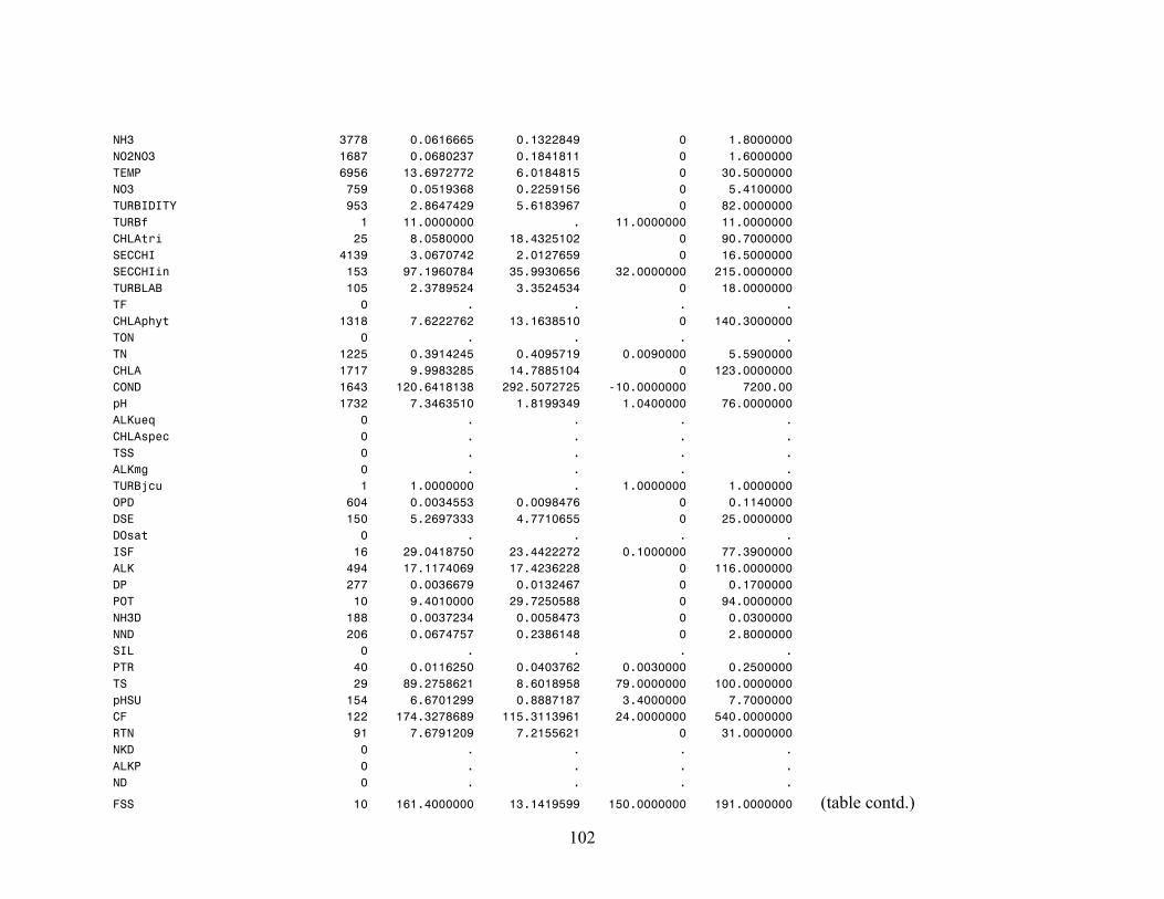
NH3 3778 0.0616665 0.1322849 0 1.8000000 NO2NO3 1687 0.0680237 0.1841811 0 1.6000000 TEMP 6956 13.6972772 6.0184815 0 30.5000000 NO3 759 0.0519368 0.2259156 0 5.4100000 TURBIDITY 953 2.8647429 5.6183967 0 82.0000000 TURBf 1 11.0000000 . 11.0000000 11.0000000 CHLAtri 25 8.0580000 18.4325102 0 90.7000000 SECCHI 4139 3.0670742 2.0127659 0 16.5000000 SECCHIin 153 97.1960784 35.9930656 32.0000000 215.0000000 TURBLAB 105 2.3789524 3.3524534 0 18.0000000 TF 0 . . . . CHLAphyt 1318 7.6222762 13.1638510 0 140.3000000 TON 0 . . . . TN 1225 0.3914245 0.4095719 0.0090000 5.5900000 CHLA 1717 9.9983285 14.7885104 0 123.0000000 COND 1643 120.6418138 292.5072725 -10.0000000 7200.00 pH 1732 7.3463510 1.8199349 1.0400000 76.0000000 ALKueq 0 . . . . CHLAspec 0 . . . . TSS 0 . . . . ALKmg 0 . . . . TURBjcu 1 1.0000000 . 1.0000000 1.0000000 OPD 604 0.0034553 0.0098476 0 0.1140000 DSE 150 5.2697333 4.7710655 0 25.0000000 DOsat 0 . . . . ISF 16 29.0418750 23.4422272 0.1000000 77.3900000 ALK 494 17.1174069 17.4236228 0 116.0000000 DP 277 0.0036679 0.0132467 0 0.1700000 POT 10 9.4010000 29.7250588 0 94.0000000 NH3D 188 0.0037234 0.0058473 0 0.0300000 NND 206 0.0674757 0.2386148 0 2.8000000 SIL 0 . . . . PTR 40 0.0116250 0.0403762 0.0030000 0.2500000 TS 29 89.2758621 8.6018958 79.0000000 100.0000000 pHSU 154 6.6701299 0.8887187 3.4000000 7.7000000 CF 122 174.3278689 115.3113961 24.0000000 540.0000000 RTN 91 7.6791209 7.2155621 0 31.0000000 NKD 0 . . . . ALKP 0 . . . . ND 0 . . . .
FSS 10 161.4000000 13.1419599 150.0000000 191.0000000 (table contd.)
102

SDunfil 8 8.5937500 8.1776454 1.5000000 21.5000000 MDS 0 . . . . ƒƒƒƒƒƒƒƒƒƒƒƒƒƒƒƒƒƒƒƒƒƒƒƒƒƒƒƒƒƒƒƒƒƒƒƒƒƒƒƒƒƒƒƒƒƒƒƒƒƒƒƒƒƒƒƒƒƒƒƒƒƒƒƒƒƒƒƒƒƒƒƒƒƒƒƒƒƒƒƒƒƒƒƒƒƒƒƒƒƒƒƒƒƒƒƒ Ecoregion 3 The MEANS Procedure Variable Label N Mean Std Dev Minimum Maximum ƒƒƒƒƒƒƒƒƒƒƒƒƒƒƒƒƒƒƒƒƒƒƒƒƒƒƒƒƒƒƒƒƒƒƒƒƒƒƒƒƒƒƒƒƒƒƒƒƒƒƒƒƒƒƒƒƒƒƒƒƒƒƒƒƒƒƒƒƒƒƒƒƒƒƒƒƒƒƒƒƒƒƒƒƒƒƒƒƒƒƒƒƒƒƒƒ SAMPLING_DATE SAMPLING_DATE 3001 1071082950 69049397.35 948153600 1243209600 TP 2803 0.0810963 0.1439799 0 2.0300000 NO2 55 0.0071091 0.0080385 0.0010000 0.0500000 DO 2330 7.0891502 2.6507863 0.1000000 14.5000000 TKN 1529 0.6097646 0.5258962 0.0100000 5.1200000 NH3 2578 0.0695132 0.1794231 0 2.1700000 NO2NO3 290 0.5860069 0.7738849 0.0010000 2.3100000 TEMP 2508 17.0769537 5.5817108 0.4000000 31.0000000 NO3 47 0.1787234 0.2550884 0.0050000 0.9600000 TURBIDITY 597 8.0212730 16.2099905 0 150.0000000 TURBf 15 18.6733333 25.2097336 3.3000000 94.1000000 CHLAtri 37 23.4637838 32.8509830 0.6000000 131.0000000 SECCHI 1128 2.1203014 1.5756308 0 7.9000000 SECCHIin 40 54.6250000 22.4929476 18.0000000 100.0000000 TURBLAB 73 5.9671233 11.2669139 0.5000000 52.0000000 TF 0 . . . . CHLAphyt 1045 11.5380861 19.4087674 0 154.2000000 TON 1 2.5000000 . 2.5000000 2.5000000 TN 0 . . . . CHLA 36 24.8666667 20.8247655 0.7000000 80.0000000 COND 64 423.3046875 87.0817267 3.0000000 615.0000000 pH 155 8.2074839 0.3926956 6.3000000 9.3000000 ALKueq 0 . . . . CHLAspec 0 . . . . TSS 0 . . . . ALKmg 0 . . . . TURBjcu 0 . . . . OPD 140 0.0628643 0.0699994 0 0.6350000 DSE 140 6.5571429 14.9739685 2.0000000 167.0000000
DOsat 0 . . . . (table contd.)
103

ISF 0 . . . . ALK 1 0.0300000 . 0.0300000 0.0300000 DP 0 . . . . POT 0 . . . . NH3D 0 . . . . NND 0 . . . . SIL 0 . . . . PTR 0 . . . . TS 0 . . . . pHSU 0 . . . . CF 0 . . . . RTN 0 . . . . NKD 0 . . . . ALKP 0 . . . . ND 0 . . . . FSS 0 . . . . SDunfil 0 . . . . MDS 0 . . . . ƒƒƒƒƒƒƒƒƒƒƒƒƒƒƒƒƒƒƒƒƒƒƒƒƒƒƒƒƒƒƒƒƒƒƒƒƒƒƒƒƒƒƒƒƒƒƒƒƒƒƒƒƒƒƒƒƒƒƒƒƒƒƒƒƒƒƒƒƒƒƒƒƒƒƒƒƒƒƒƒƒƒƒƒƒƒƒƒƒƒƒƒƒƒƒƒ Ecoregion 4 The MEANS Procedure Variable Label N Mean Std Dev Minimum Maximum ƒƒƒƒƒƒƒƒƒƒƒƒƒƒƒƒƒƒƒƒƒƒƒƒƒƒƒƒƒƒƒƒƒƒƒƒƒƒƒƒƒƒƒƒƒƒƒƒƒƒƒƒƒƒƒƒƒƒƒƒƒƒƒƒƒƒƒƒƒƒƒƒƒƒƒƒƒƒƒƒƒƒƒƒƒƒƒƒƒƒƒƒƒƒƒƒ SAMPLING_DATE SAMPLING_DATE 2373 1055808000 84637860.29 465523200 1215561600 TP 1525 0.0849016 0.1357922 0 1.6600000 NO2 676 0.0121612 0.0223142 0.0010000 0.3000000 DO 813 7.6377614 2.3967986 0.1000000 14.4000000 TKN 1235 0.7572955 0.7315680 0 5.2000000 NH3 1366 0.1049458 0.2015044 0 2.0700000 NO2NO3 1136 0.2120352 0.3283756 0 1.9700000 TEMP 1300 18.9302154 6.9499424 0.1000000 31.0000000 NO3 165 0.3350303 0.4472315 0 1.8000000 TURBIDITY 659 11.1980273 17.6021935 0.3000000 170.0000000 TURBf 78 33.9910256 25.7105526 4.9000000 161.2000000 CHLAtri 0 . . . . SECCHI 817 1.8675765 1.4475689 0.1000000 7.0000000
SECCHIin 299 75.8026756 49.1738239 2.0000000 214.0000000 (table contd.)
104

105
TURBLAB 27 50.2333333 49.8819298 2.2000000 190.0000000 TF 0 . . . . CHLAphyt 220 16.0907273 18.7107064 0.2000000 104.7000000 TON 0 . . . . TN 0 . . . . CHLA 0 . . . . COND 17 7613.12 10677.37 368.0000000 45100.00 pH 19 8.0531579 1.0515547 4.4200000 9.4300000 ALKueq 0 . . . . CHLAspec 0 . . . . TSS 0 . . . . ALKmg 0 . . . . TURBjcu 0 . . . . OPD 0 . . . . DSE 0 . . . . DOsat 0 . . . . ISF 1 0 . 0 0 ALK 0 . . . . DP 0 . . . . POT 0 . . . . NH3D 0 . . . . NND 0 . . . . SIL 0 . . . . PTR 0 . . . . TS 0 . . . . pHSU 0 . . . . CF 0 . . . . RTN 0 . . . . NKD 0 . . . . ALKP 0 . . . . ND 0 . . . . FSS 0 . . . . SDunfil 0 . . . . MDS 0 . . . . ƒƒƒƒƒƒƒƒƒƒƒƒƒƒƒƒƒƒƒƒƒƒƒƒƒƒƒƒƒƒƒƒƒƒƒƒƒƒƒƒƒƒƒƒƒƒƒƒƒƒƒƒƒƒƒƒƒƒƒƒƒƒƒƒƒƒƒƒƒƒƒƒƒƒƒƒƒƒƒƒƒƒƒƒƒƒƒƒƒƒƒƒƒƒƒƒ

Ecoregion 5 The MEANS Procedure Variable Label N Mean Std Dev Minimum Maximum ƒƒƒƒƒƒƒƒƒƒƒƒƒƒƒƒƒƒƒƒƒƒƒƒƒƒƒƒƒƒƒƒƒƒƒƒƒƒƒƒƒƒƒƒƒƒƒƒƒƒƒƒƒƒƒƒƒƒƒƒƒƒƒƒƒƒƒƒƒƒƒƒƒƒƒƒƒƒƒƒƒƒƒƒƒƒƒƒƒƒƒƒƒƒƒƒ SAMPLING_DATE SAMPLING_DATE 2732 1053944201 92990096.10 455932800 1215475200 TP 2147 0.1362948 0.4014982 0 6.8300000 NO2 796 0.0202563 0.0293580 0.0010000 0.3000000 DO 1021 7.2124976 2.9037959 0.0500000 20.0000000 TKN 1927 1.0244369 1.0396480 0 22.5000000 NH3 1543 0.1231905 0.2208612 0 2.0000000 NO2NO3 1560 0.1998846 0.3824704 0 6.5000000 TEMP 1733 19.9669359 7.1293248 0.2000000 31.0000000 NO3 128 0.6865234 1.9325773 0 18.0600000 TURBIDITY 621 18.1658615 25.7178429 0.4000000 180.0000000 TURBf 63 25.9365079 32.9551421 2.3000000 150.0000000 CHLAtri 0 . . . . SECCHI 705 1.3630071 1.2700294 0.1000000 7.3000000 SECCHIin 318 57.3333333 47.2571550 1.0000000 216.0000000 TURBLAB 42 18.9428571 13.0223287 2.0000000 64.0000000 TF 9 66.7444444 11.4269540 40.1000000 79.4000000 CHLAphyt 228 27.5338158 28.9253675 0.5000000 129.2000000 TON 0 . . . . TN 0 . . . . CHLA 0 . . . . COND 16 3276.69 2365.50 917.0000000 8650.00 pH 15 8.4893333 0.6620473 7.4100000 9.6000000 ALKueq 0 . . . . CHLAspec 0 . . . . TSS 0 . . . . ALKmg 0 . . . . TURBjcu 0 . . . . OPD 0 . . . . DSE 0 . . . . DOsat 0 . . . . ISF 2 0 0 0 0 ALK 4 29.0000000 0 29.0000000 29.0000000 DP 0 . . . . POT 0 . . . .
NH3D 0 . . . . (table contd.)
106
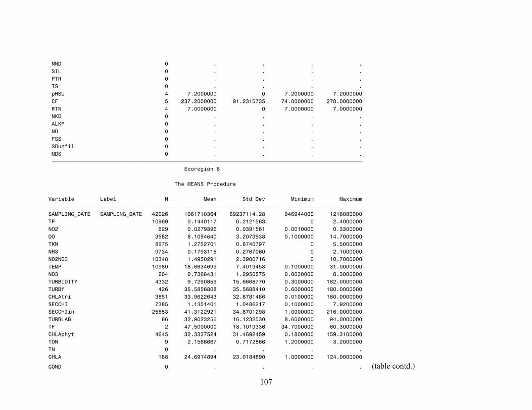
NND 0 . . . . SIL 0 . . . . PTR 0 . . . . TS 0 . . . . pHSU 4 7.2000000 0 7.2000000 7.2000000 CF 5 237.2000000 91.2315735 74.0000000 278.0000000 RTN 4 7.0000000 0 7.0000000 7.0000000 NKD 0 . . . . ALKP 0 . . . . ND 0 . . . . FSS 0 . . . . SDunfil 0 . . . . MDS 0 . . . . ƒƒƒƒƒƒƒƒƒƒƒƒƒƒƒƒƒƒƒƒƒƒƒƒƒƒƒƒƒƒƒƒƒƒƒƒƒƒƒƒƒƒƒƒƒƒƒƒƒƒƒƒƒƒƒƒƒƒƒƒƒƒƒƒƒƒƒƒƒƒƒƒƒƒƒƒƒƒƒƒƒƒƒƒƒƒƒƒƒƒƒƒƒƒƒƒ Ecoregion 6 The MEANS Procedure Variable Label N Mean Std Dev Minimum Maximum ƒƒƒƒƒƒƒƒƒƒƒƒƒƒƒƒƒƒƒƒƒƒƒƒƒƒƒƒƒƒƒƒƒƒƒƒƒƒƒƒƒƒƒƒƒƒƒƒƒƒƒƒƒƒƒƒƒƒƒƒƒƒƒƒƒƒƒƒƒƒƒƒƒƒƒƒƒƒƒƒƒƒƒƒƒƒƒƒƒƒƒƒƒƒƒƒƒ SAMPLING_DATE SAMPLING_DATE 42026 1061710364 69237114.28 946944000 1216080000 TP 10969 0.1440117 0.2121563 0 2.4000000 NO2 629 0.0279396 0.0391561 0.0010000 0.3300000 DO 3582 8.1094640 3.2073938 0.1000000 14.7000000 TKN 8275 1.2752701 0.8740797 0 5.5000000 NH3 9734 0.1793115 0.2767060 0 2.1000000 NO2NO3 10348 1.4950291 2.3900716 0 10.7000000 TEMP 10980 18.6634699 7.4019453 0.1000000 31.0000000 NO3 204 0.7368431 1.2950575 0.0030000 8.3000000 TURBIDITY 4332 9.7290859 15.6668770 0.3000000 182.0000000 TURBf 426 35.5856808 35.5688410 0.6000000 180.0000000 CHLAtri 3851 33.9622643 32.8781486 0.0100000 160.0000000 SECCHI 7385 1.1351401 1.0486217 0.1000000 7.9200000 SECCHIin 25553 41.3122921 34.8701298 1.0000000 216.0000000 TURBLAB 86 32.9023256 16.1232530 8.6000000 94.0000000 TF 2 47.5000000 18.1019336 34.7000000 60.3000000 CHLAphyt 4645 32.3337524 31.4692459 0.1800000 159.3100000 TON 9 2.1566667 0.7172866 1.2000000 3.2000000 TN 0 . . . . CHLA 188 24.6914894 23.0184890 1.0000000 124.0000000
COND 0 . . . . (table contd.)
107

pH 0 . . . . ALKueq 0 . . . . CHLAspec 0 . . . . TSS 0 . . . . ALKmg 0 . . . . TURBjcu 749 28.8875834 28.0853606 1.0000000 280.0000000 OPD 0 . . . . DSE 0 . . . . DOsat 0 . . . . ISF 0 . . . . ALK 0 . . . . DP 0 . . . . POT 0 . . . . NH3D 0 . . . . NND 0 . . . . SIL 0 . . . . PTR 0 . . . . TS 0 . . . . pHSU 0 . . . . CF 0 . . . . RTN 0 . . . . NKD 0 . . . . ALKP 0 . . . . ND 0 . . . . FSS 0 . . . . SDunfil 0 . . . . MDS 0 . . . . ƒƒƒƒƒƒƒƒƒƒƒƒƒƒƒƒƒƒƒƒƒƒƒƒƒƒƒƒƒƒƒƒƒƒƒƒƒƒƒƒƒƒƒƒƒƒƒƒƒƒƒƒƒƒƒƒƒƒƒƒƒƒƒƒƒƒƒƒƒƒƒƒƒƒƒƒƒƒƒƒƒƒƒƒƒƒƒƒƒƒƒƒƒƒƒƒƒ Ecoregion 7 The MEANS Procedure Variable Label N Mean Std Dev Minimum Maximum ƒƒƒƒƒƒƒƒƒƒƒƒƒƒƒƒƒƒƒƒƒƒƒƒƒƒƒƒƒƒƒƒƒƒƒƒƒƒƒƒƒƒƒƒƒƒƒƒƒƒƒƒƒƒƒƒƒƒƒƒƒƒƒƒƒƒƒƒƒƒƒƒƒƒƒƒƒƒƒƒƒƒƒƒƒƒƒƒƒƒƒƒƒƒƒƒƒ SAMPLING_DATE SAMPLING_DATE 95959 1066886436 107390156 286329600 1256083200 TP 43163 0.0966367 0.1846405 0 3.8000000 NO2 802 0.0119925 0.0202864 0 0.3200000 DO 23363 7.3870535 3.8782855 0.0500000 14.7000000
TKN 18115 1.1829616 0.7638099 0 5.5000000 (table contd.)
108

NH3 8840 0.1833612 0.3468874 0 2.1700000 NO2NO3 11717 0.3528088 1.0588926 -0.0600000 11.9000000 TEMP 31472 16.1549346 7.1289453 0 31.0000000 NO3 540 0.0710370 0.3532226 0.0030000 7.8000000 TURBIDITY 10124 6.1682339 10.1446756 0.1000000 190.0000000 TURBf 645 15.7683721 14.3117722 0.4000000 95.0000000 CHLAtri 8853 22.9962521 28.4140835 0.0100000 160.3200000 SECCHI 67745 2.6243479 1.7663243 0 14.3000000 SECCHIin 2681 71.2651996 50.9047341 1.0000000 216.0000000 TURBLAB 382 15.3073298 17.5532979 1.8000000 196.0000000 TF 183 53.7415301 15.4767682 32.5000000 80.0000000 CHLAphyt 9065 22.4629789 25.6432150 0.0040000 159.1300000 TON 42 1.4666667 0.6237834 0.5000000 2.8000000 TN 3908 0.5954831 3.3062136 0.0200000 205.8000000 CHLA 6277 8.0731963 15.2203786 0.1100000 607.0000000 COND 199 184.0502513 59.5321616 47.0000000 570.0000000 pH 2550 7.7703804 0.4295751 4.9000000 9.6600000 ALKueq 1 1764.56 . 1764.56 1764.56 CHLAspec 2279 10.8478412 26.4008527 0.3000000 247.0000000 TSS 3459 1.7235230 2.4989853 0 36.9000000 ALKmg 1263 50.8989311 11.3675744 21.3000000 104.5000000 TURBjcu 0 . . . . OPD 75 0.0349333 0.0364886 0.0100000 0.1700000 DSE 0 . . . . DOsat 0 . . . . ISF 0 . . . . ALK 1137 52.3948989 20.9924049 1.0000000 273.0000000 DP 3675 0.0089189 0.0078251 0 0.1100000 POT 371 0.6088113 8.2118085 0 112.0000000 NH3D 37 0.1270270 0.0732145 0.1000000 0.5000000 NND 37 0.3297297 0.2601974 0.1000000 1.0000000 SIL 3443 1.5629448 1.1738694 0.0500000 6.7200000 PTR 0 . . . . TS 3 139.6666667 26.2741952 124.0000000 170.0000000 pHSU 1137 7.1012313 0.3313150 5.8000000 9.1000000 CF 252 206.9880952 77.3295057 52.0000000 650.0000000 RTN 161 13.8807453 26.2592782 0.8000000 239.0000000 NKD 34 0.9647059 0.5515171 0.2000000 1.9000000 ALKP 4 12.0000000 0 12.0000000 12.0000000 ND 0 . . . .
FSS 0 . . . . (table contd.)
109
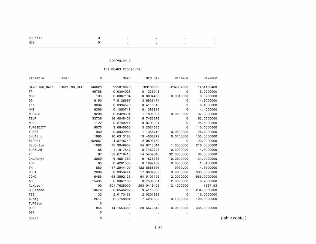
SDunfil 0 . . . . MDS 0 . . . . ƒƒƒƒƒƒƒƒƒƒƒƒƒƒƒƒƒƒƒƒƒƒƒƒƒƒƒƒƒƒƒƒƒƒƒƒƒƒƒƒƒƒƒƒƒƒƒƒƒƒƒƒƒƒƒƒƒƒƒƒƒƒƒƒƒƒƒƒƒƒƒƒƒƒƒƒƒƒƒƒƒƒƒƒƒƒƒƒƒƒƒƒƒƒƒƒƒ Ecoregion 8 The MEANS Procedure Variable Label N Mean Std Dev Minimum Maximum ƒƒƒƒƒƒƒƒƒƒƒƒƒƒƒƒƒƒƒƒƒƒƒƒƒƒƒƒƒƒƒƒƒƒƒƒƒƒƒƒƒƒƒƒƒƒƒƒƒƒƒƒƒƒƒƒƒƒƒƒƒƒƒƒƒƒƒƒƒƒƒƒƒƒƒƒƒƒƒƒƒƒƒƒƒƒƒƒƒƒƒƒƒƒƒƒƒƒ SAMPLING_DATE SAMPLING_DATE 146623 955810070 189186600 -234057600 1251158400 TP 46788 0.0304025 0.1236048 0 15.0000000 NO2 103 0.0087184 0.0094458 0.0010000 0.0700000 DO 6150 7.5126667 3.6835174 0 14.6000000 TKN 9084 0.3994570 0.4115512 0 6.1000000 NH3 6356 0.1050746 0.1383819 0 4.4000000 NO2NO3 9208 0.2328394 1.1898907 -0.0500000 67.0000000 TEMP 33736 16.4048405 6.7453273 0 62.0000000 NO3 1122 0.2730214 0.8793994 0 25.5000000 TURBIDITY 9075 3.0845950 3.2021525 0 110.0000000 TURBf 960 0.8032083 1.1356710 0.0800000 26.7000000 CHLAtri 1995 10.6313183 13.4006272 0.0100000 155.0000000 SECCHI 102067 4.3748740 2.0893759 0 23.0000000 SECCHIin 1082 75.3049908 54.8713014 1.0000000 216.0000000 TURBLAB 85 1.1917647 0.7467727 0.3000000 4.6000000 TF 67 52.6716418 14.5439648 32.0000000 80.0000000 CHLAphyt 2059 6.4681350 9.1875785 0.0600000 131.0000000 TON 65 0.4201538 0.1897489 0.0500000 1.0400000 TN 560 -17.2944107 422.5588666 -9999.00 4.6500000 CHLA 2088 8.3959444 17.6082905 0.0600000 305.0000000 COND 6485 64.3592136 64.5107199 2.0000000 956.0000000 pH 15495 6.3067189 0.7599801 2.9600000 9.7300000 ALKueq 100 201.7628000 293.0419409 -12.4200000 1897.53 CHLAspec 18676 6.6546262 9.4119963 0 234.8000000 TSS 132 2.0170455 2.5201238 0 16.0000000 ALKmg 2617 6.1758884 7.4283608 0.1000000 120.0000000 TURBjcu 0 . . . . OPD 844 14.1553389 20.5673612 0.0100000 335.0000000 DSE 0 . . . .
DOsat 0 . . . . (table contd.)
110

ISF 2 5.0000000 0 5.0000000 5.0000000 ALK 13211 10.0312391 16.3272221 0 193.7000000 DP 211 0.000772512 0.0041122 0 0.0340000 POT 32 9.8750000 31.3314744 0 112.0000000 NH3D 12 0.1333333 0.0492366 0.1000000 0.2000000 NND 12 0.3250000 0.1138180 0.2000000 0.5000000 SIL 1 3.4000000 . 3.4000000 3.4000000 PTR 0 . . . . TS 653 31.9401225 27.1884152 0 230.0000000 pHSU 6902 6.2103448 0.5629097 3.4000000 8.1000000 CF 6364 49.5367693 30.2389312 20.0000000 851.0000000 RTN 3075 4.1438699 5.2051640 0 127.0000000 NKD 9 0.7000000 0.4743416 0.3000000 1.5000000 ALKP 0 . . . . ND 1202 0.0882404 0.1267311 0.0070000 0.9400000 FSS 0 . . . . SDunfil 0 . . . . MDS 0 . . . . ƒƒƒƒƒƒƒƒƒƒƒƒƒƒƒƒƒƒƒƒƒƒƒƒƒƒƒƒƒƒƒƒƒƒƒƒƒƒƒƒƒƒƒƒƒƒƒƒƒƒƒƒƒƒƒƒƒƒƒƒƒƒƒƒƒƒƒƒƒƒƒƒƒƒƒƒƒƒƒƒƒƒƒƒƒƒƒƒƒƒƒƒƒƒƒƒƒ Ecoregion 9 The MEANS Procedure Variable Label N Mean Std Dev Minimum Maximum ƒƒƒƒƒƒƒƒƒƒƒƒƒƒƒƒƒƒƒƒƒƒƒƒƒƒƒƒƒƒƒƒƒƒƒƒƒƒƒƒƒƒƒƒƒƒƒƒƒƒƒƒƒƒƒƒƒƒƒƒƒƒƒƒƒƒƒƒƒƒƒƒƒƒƒƒƒƒƒƒƒƒƒƒƒƒƒƒƒƒƒƒƒƒƒƒƒ SAMPLING_DATE SAMPLING_DATE 37210 1049009892 106340822 326505600 1216080000 TP 20247 0.1102134 0.9063010 0 59.0000000 NO2 3513 0.0185989 0.0294614 0 0.3300000 DO 10361 7.9556269 2.5000834 0 17.2000000 TKN 14676 0.6713219 0.5798187 0 5.4200000 NH3 15157 0.1212204 0.2372204 0 2.1400000 NO2NO3 13728 0.2334268 0.5247336 0 10.2000000 TEMP 16111 20.7822469 7.2177746 0.1000000 36.4000000 NO3 4019 0.5959473 1.4709105 0 52.8700000 TURBIDITY 8151 11.7404122 17.5039062 0.3000000 190.0000000 TURBf 434 14.9923963 20.7341550 1.2000000 191.3000000 CHLAtri 3474 26.4100835 29.9299757 0 160.5500000 SECCHI 6510 1.1311982 0.8978058 0.1000000 7.8000000
SECCHIin 14687 37.3150405 30.1701937 1.0000000 216.0000000 (table contd.)
111

112
TURBLAB 1282 27.7706708 31.2726043 0.5000000 190.0000000 TF 45 59.6155556 11.0566096 42.0000000 77.9000000 CHLAphyt 2944 27.8866033 31.0131540 0 159.1300000 TON 1565 1.7498256 13.9156596 0 230.0000000 TN 3768 1.0806054 9.0005369 0 230.1000000 CHLA 4299 15.1833217 17.8160011 0.2000000 133.0000000 COND 1084 96.4176107 228.4740454 1.4000000 3200.00 pH 1191 6.6982116 1.2549935 3.4000000 10.5000000 ALKueq 0 . . . . CHLAspec 0 . . . . TSS 715 14.9174825 25.1486675 0 312.0000000 ALKmg 918 23.5549564 20.4030615 0 120.0000000 TURBjcu 23 7.0347826 6.0007279 1.4000000 25.0000000 OPD 0 . . . . DSE 0 . . . . DOsat 1404 79.4281467 27.1787739 0 220.4000000 ISF 20 3.5030000 3.3364196 0.0200000 12.2000000 ALK 0 . . . . DP 0 . . . . POT 0 . . . . NH3D 0 . . . . NND 0 . . . . SIL 0 . . . . PTR 0 . . . . TS 0 . . . . pHSU 0 . . . . CF 0 . . . . RTN 0 . . . . NKD 0 . . . . ALKP 0 . . . . ND 0 . . . . FSS 0 . . . . SDunfil 0 . . . . MDS 0 . . . . ƒƒƒƒƒƒƒƒƒƒƒƒƒƒƒƒƒƒƒƒƒƒƒƒƒƒƒƒƒƒƒƒƒƒƒƒƒƒƒƒƒƒƒƒƒƒƒƒƒƒƒƒƒƒƒƒƒƒƒƒƒƒƒƒƒƒƒƒƒƒƒƒƒƒƒƒƒƒƒƒƒƒƒƒƒƒƒƒƒƒƒƒƒƒƒƒƒ

Ecoregion 10 The MEANS Procedure Variable Label N Mean Std Dev Minimum Maximum ƒƒƒƒƒƒƒƒƒƒƒƒƒƒƒƒƒƒƒƒƒƒƒƒƒƒƒƒƒƒƒƒƒƒƒƒƒƒƒƒƒƒƒƒƒƒƒƒƒƒƒƒƒƒƒƒƒƒƒƒƒƒƒƒƒƒƒƒƒƒƒƒƒƒƒƒƒƒƒƒƒƒƒƒƒƒƒƒƒƒƒƒƒƒƒƒ SAMPLING_DATE SAMPLING_DATE 1452 1066307861 74097532.35 947376000 1205107200 TP 1354 0.1218936 0.1244424 0.0050000 1.1300000 NO2 130 0.0235769 0.0255955 0.0050000 0.1000000 DO 1227 8.0116544 2.3434723 0.1000000 14.5000000 TKN 1082 0.8502865 0.5355254 0.0500000 4.5900000 NH3 463 0.0765983 0.1714552 0.0050000 1.7000000 NO2NO3 1274 0.1665581 0.4299151 0.0050000 9.0200000 TEMP 1251 21.3302158 7.2079510 3.0000000 31.0000000 NO3 0 . . . . TURBIDITY 64 39.6406250 33.9539170 4.4000000 140.0000000 TURBf 0 . . . . CHLAtri 19 94.8521053 31.5054931 49.6100000 155.2000000 SECCHI 65 0.2544615 0.1175536 0.1000000 0.6500000 SECCHIin 709 26.9985896 21.8326001 1.0000000 172.0000000 TURBLAB 813 18.3217712 29.5015468 0.5000000 190.0000000 TF 0 . . . . CHLAphyt 19 90.7589474 32.8603528 45.3900000 157.5700000 TON 0 . . . . TN 0 . . . . CHLA 7 77.4428571 47.8074909 7.1000000 126.2000000 COND 0 . . . . pH 0 . . . . ALKueq 0 . . . . CHLAspec 0 . . . . TSS 0 . . . . ALKmg 0 . . . . TURBjcu 0 . . . . OPD 0 . . . . DSE 0 . . . . DOsat 0 . . . . ISF 0 . . . . ALK 0 . . . . DP 0 . . . . POT 0 . . . .
NH3D 0 . . . . (table contd.)
113

NND 0 . . . . SIL 0 . . . . PTR 0 . . . . TS 0 . . . . pHSU 0 . . . . CF 0 . . . . RTN 0 . . . . NKD 0 . . . . ALKP 0 . . . . ND 0 . . . . FSS 0 . . . . SDunfil 0 . . . . MDS 0 . . . . ƒƒƒƒƒƒƒƒƒƒƒƒƒƒƒƒƒƒƒƒƒƒƒƒƒƒƒƒƒƒƒƒƒƒƒƒƒƒƒƒƒƒƒƒƒƒƒƒƒƒƒƒƒƒƒƒƒƒƒƒƒƒƒƒƒƒƒƒƒƒƒƒƒƒƒƒƒƒƒƒƒƒƒƒƒƒƒƒƒƒƒƒƒƒƒƒ Ecoregion 11 The MEANS Procedure Variable Label N Mean Std Dev Minimum Maximum ƒƒƒƒƒƒƒƒƒƒƒƒƒƒƒƒƒƒƒƒƒƒƒƒƒƒƒƒƒƒƒƒƒƒƒƒƒƒƒƒƒƒƒƒƒƒƒƒƒƒƒƒƒƒƒƒƒƒƒƒƒƒƒƒƒƒƒƒƒƒƒƒƒƒƒƒƒƒƒƒƒƒƒƒƒƒƒƒƒƒƒƒƒƒƒƒƒ SAMPLING_DATE SAMPLING_DATE 19525 950356094 231976334 286329600 1222560000 TP 8783 0.0388849 0.0712246 0 0.9100000 NO2 1534 0.0094465 0.0119808 0 0.1700000 DO 3286 8.0710590 2.9990175 0 104.0000000 TKN 7673 0.4035996 0.4609487 0 6.9000000 NH3 4973 0.1551172 0.2406584 0 2.1200000 NO2NO3 8156 0.4103352 7.2067355 0 650.0000000 TEMP 16490 16.9344269 7.7076708 0 83.2000000 NO3 1121 0.4071142 0.7460818 0 8.6600000 TURBIDITY 7303 6.4471724 20.0797205 0.1000000 1340.00 TURBf 945 15.1442328 22.4935525 0.5000000 190.0000000 CHLAtri 2012 8.5041501 12.3315369 0.1000000 120.8900000 SECCHI 3039 2.1701711 1.2855456 0.1000000 7.9000000 SECCHIin 5848 100.4151847 61.5665955 1.0000000 288.0000000 TURBLAB 363 15.9407713 27.1384295 0.5000000 197.0000000 TF 94 62.9734043 9.3087792 50.6000000 79.2000000 CHLAphyt 5056 8.0970214 12.3828825 0.2000000 254.5200000 TON 100 0.4821000 0.3346830 0.0400000 1.6500000
TN 61 0.7877049 0.6312062 0.1200000 2.6400000 (table contd.)
114

CHLA 437 8.1123570 18.8589869 0.4000000 152.6000000 COND 5622 181.1010317 153.4829883 33.0000000 1273.00 pH 6596 6.9021149 1.1734227 2.8000000 74.0000000 ALKueq 0 . . . . CHLAspec 0 . . . . TSS 0 . . . . ALKmg 0 . . . . TURBjcu 3 39.1000000 65.7313472 1.1000000 115.0000000 OPD 2891 0.1301263 1.3082043 0.0090000 20.0000000 DSE 0 . . . . DOsat 0 . . . . ISF 6 6.1833333 8.8481448 0.2000000 23.0000000 ALK 9627 26.2778851 27.0290516 0 224.0000000 DP 179 0.0110056 0.0368735 0 0.4000000 POT 13 65.8461538 54.6410196 0 112.0000000 NH3D 247 0.0218623 0.0113595 0.0200000 0.1000000 NND 247 0.3141700 0.0826493 0.2000000 0.7000000 SIL 0 . . . . PTR 0 . . . . TS 2663 127.1013894 104.3823640 4.0000000 872.0000000 pHSU 5432 6.3056701 1.0157610 2.6000000 9.0000000 CF 2181 187.7661623 204.9200501 22.0000000 1750.00 RTN 1375 6.0553455 20.0256684 0 476.0000000 NKD 1044 0.3066188 0.6554630 0.0200000 2.0000000 ALKP 0 . . . . ND 0 . . . . FSS 0 . . . . SDunfil 133 5.9247744 6.1244149 0.5800000 47.5000000 MDS 25 18.8640000 24.0026887 0.6000000 87.0000000 ƒƒƒƒƒƒƒƒƒƒƒƒƒƒƒƒƒƒƒƒƒƒƒƒƒƒƒƒƒƒƒƒƒƒƒƒƒƒƒƒƒƒƒƒƒƒƒƒƒƒƒƒƒƒƒƒƒƒƒƒƒƒƒƒƒƒƒƒƒƒƒƒƒƒƒƒƒƒƒƒƒƒƒƒƒƒƒƒƒƒƒƒƒƒƒƒƒ Ecoregion 12 The MEANS Procedure Variable Label N Mean Std Dev Minimum Maximum ƒƒƒƒƒƒƒƒƒƒƒƒƒƒƒƒƒƒƒƒƒƒƒƒƒƒƒƒƒƒƒƒƒƒƒƒƒƒƒƒƒƒƒƒƒƒƒƒƒƒƒƒƒƒƒƒƒƒƒƒƒƒƒƒƒƒƒƒƒƒƒƒƒƒƒƒƒƒƒƒƒƒƒƒƒƒƒƒƒƒƒƒƒƒƒƒƒƒ SAMPLING_DATE SAMPLING_DATE 176588 973999659 186903935 315964800 1211155200 TP 150597 0.0700447 0.5718296 0 203.0000000
NO2 7295 0.0050647 0.0065821 0 0.1900000 (table contd.)
115
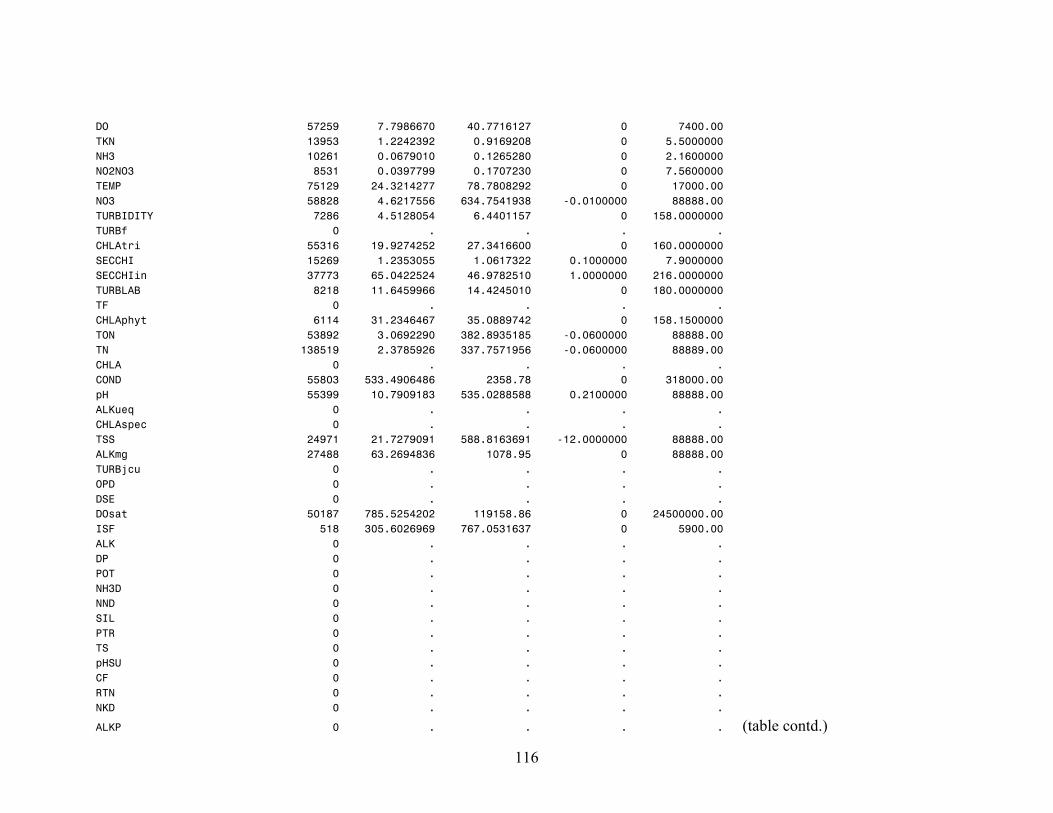
DO 57259 7.7986670 40.7716127 0 7400.00 TKN 13953 1.2242392 0.9169208 0 5.5000000 NH3 10261 0.0679010 0.1265280 0 2.1600000 NO2NO3 8531 0.0397799 0.1707230 0 7.5600000 TEMP 75129 24.3214277 78.7808292 0 17000.00 NO3 58828 4.6217556 634.7541938 -0.0100000 88888.00 TURBIDITY 7286 4.5128054 6.4401157 0 158.0000000 TURBf 0 . . . . CHLAtri 55316 19.9274252 27.3416600 0 160.0000000 SECCHI 15269 1.2353055 1.0617322 0.1000000 7.9000000 SECCHIin 37773 65.0422524 46.9782510 1.0000000 216.0000000 TURBLAB 8218 11.6459966 14.4245010 0 180.0000000 TF 0 . . . . CHLAphyt 6114 31.2346467 35.0889742 0 158.1500000 TON 53892 3.0692290 382.8935185 -0.0600000 88888.00 TN 138519 2.3785926 337.7571956 -0.0600000 88889.00 CHLA 0 . . . . COND 55803 533.4906486 2358.78 0 318000.00 pH 55399 10.7909183 535.0288588 0.2100000 88888.00 ALKueq 0 . . . . CHLAspec 0 . . . . TSS 24971 21.7279091 588.8163691 -12.0000000 88888.00 ALKmg 27488 63.2694836 1078.95 0 88888.00 TURBjcu 0 . . . . OPD 0 . . . . DSE 0 . . . . DOsat 50187 785.5254202 119158.86 0 24500000.00 ISF 518 305.6026969 767.0531637 0 5900.00 ALK 0 . . . . DP 0 . . . . POT 0 . . . . NH3D 0 . . . . NND 0 . . . . SIL 0 . . . . PTR 0 . . . . TS 0 . . . . pHSU 0 . . . . CF 0 . . . . RTN 0 . . . . NKD 0 . . . .
ALKP 0 . . . . (table contd.)
116

ND 0 . . . . FSS 0 . . . . SDunfil 0 . . . . MDS 0 . . . . ƒƒƒƒƒƒƒƒƒƒƒƒƒƒƒƒƒƒƒƒƒƒƒƒƒƒƒƒƒƒƒƒƒƒƒƒƒƒƒƒƒƒƒƒƒƒƒƒƒƒƒƒƒƒƒƒƒƒƒƒƒƒƒƒƒƒƒƒƒƒƒƒƒƒƒƒƒƒƒƒƒƒƒƒƒƒƒƒƒƒƒƒƒƒƒƒƒ Ecoregion 13 The MEANS Procedure Variable Label N Mean Std Dev Minimum Maximum ƒƒƒƒƒƒƒƒƒƒƒƒƒƒƒƒƒƒƒƒƒƒƒƒƒƒƒƒƒƒƒƒƒƒƒƒƒƒƒƒƒƒƒƒƒƒƒƒƒƒƒƒƒƒƒƒƒƒƒƒƒƒƒƒƒƒƒƒƒƒƒƒƒƒƒƒƒƒƒƒƒƒƒƒƒƒƒƒƒƒƒƒƒƒƒƒƒ SAMPLING_DATE SAMPLING_DATE 21437 977116930 193760378 316569600 1210464000 TP 20730 0.1902814 10.3285810 0 1486.00 NO2 4772 0.0015136 0.0035430 0 0.1200000 DO 7372 8.2699349 25.6106987 0 1168.00 TKN 8880 1.4955079 0.5845659 0 5.4800000 NH3 130 0.0531538 0.0969593 0 0.5500000 NO2NO3 8760 0.1121220 0.1470003 0 1.2700000 TEMP 8375 24.9861337 4.6287669 2.2000000 37.0000000 NO3 13614 0.1193996 0.2784066 0 18.7900000 TURBIDITY 4916 15.9059398 18.4005552 0 155.0000000 TURBf 0 . . . . CHLAtri 3985 24.8535257 17.7445825 0 152.5000000 SECCHI 4296 0.6151304 0.3210948 0.1000000 4.2500000 SECCHIin 6 34.0000000 4.8989795 24.0000000 36.0000000 TURBLAB 24 8.1875000 9.8232339 1.0000000 38.0000000 TF 0 . . . . CHLAphyt 13 7.2153846 10.1185347 1.6000000 40.1000000 TON 16094 2.0627387 34.4829477 0 3054.00 TN 15797 2.2447495 34.8640512 0 3058.00 CHLA 6 7.2333333 6.0905391 2.2000000 18.5000000 COND 7419 1702.01 7061.09 0 54400.00 pH 7765 8.2044018 12.9973952 1.0000000 844.0000000 ALKueq 0 . . . . CHLAspec 0 . . . . TSS 4831 15.6642621 20.8519478 0.1000000 484.0000000 ALKmg 2099 114.2226489 35.2040134 1.2000000 442.0000000 TURBjcu 0 . . . .
OPD 0 . . . . (table contd.)
117

DSE 0 . . . . DOsat 4401 100.1339125 360.1639258 0 13028.00 ISF 3 0 0 0 0 ALK 0 . . . . DP 0 . . . . POT 0 . . . . NH3D 0 . . . . NND 0 . . . . SIL 0 . . . . PTR 0 . . . . TS 0 . . . . pHSU 0 . . . . CF 0 . . . . RTN 0 . . . . NKD 0 . . . . ALKP 0 . . . . ND 0 . . . . FSS 0 . . . . SDunfil 0 . . . . MDS 0 . . . . ƒƒƒƒƒƒƒƒƒƒƒƒƒƒƒƒƒƒƒƒƒƒƒƒƒƒƒƒƒƒƒƒƒƒƒƒƒƒƒƒƒƒƒƒƒƒƒƒƒƒƒƒƒƒƒƒƒƒƒƒƒƒƒƒƒƒƒƒƒƒƒƒƒƒƒƒƒƒƒƒƒƒƒƒƒƒƒƒƒƒƒƒƒƒƒƒƒ Ecoregion 14 The MEANS Procedure Variable Label N Mean Std Dev Minimum Maximum ƒƒƒƒƒƒƒƒƒƒƒƒƒƒƒƒƒƒƒƒƒƒƒƒƒƒƒƒƒƒƒƒƒƒƒƒƒƒƒƒƒƒƒƒƒƒƒƒƒƒƒƒƒƒƒƒƒƒƒƒƒƒƒƒƒƒƒƒƒƒƒƒƒƒƒƒƒƒƒƒƒƒƒƒƒƒƒƒƒƒƒƒƒƒƒƒƒ SAMPLING_DATE SAMPLING_DATE 35066 934771180 170933449 329270400 1229299200 TP 8002 0.0242129 0.0416411 0 0.7800000 NO2 178 0.0103989 0.0112206 0 0.0700000 DO 1873 8.5911372 2.1183560 0 14.3000000 TKN 2547 0.5977935 0.5163471 0.0500000 5.5000000 NH3 2414 0.0575998 0.1024775 0 1.9300000
NO2NO3 2429 1.2351770 1.7391695 0.0010000 10.4500000 (table contd.) TEMP 8504 19.6206315 5.9807921 0.3000000 31.1000000 NO3 2423 0.9927858 1.5705867 0 24.9400000 TURBIDITY 1488 4.8444220 5.7669392 0.4000000 66.0000000 TURBf 139 1.0847482 1.7020168 0.2000000 17.5000000 CHLAtri 5 26.1620000 31.9382564 5.6000000 81.8000000 SECCHI 12732 4.9280518 2.4607699 0.1000000 16.0000000
118

119
SECCHIin 1126 38.1456483 23.4261793 1.0000000 108.0000000 TURBLAB 0 . . . . TF 0 . . . . CHLAphyt 690 18.1452899 27.4795752 0.4500000 147.0000000 TON 509 0.7013360 0.5420606 0.0200000 3.6900000 TN 0 . . . . CHLA 745 15.0483758 26.6926481 0.4000000 472.0000000 COND 750 76.6857867 63.8363787 2.0000000 688.0000000 pH 16077 6.4529626 0.8394406 3.6000000 10.7000000 ALKueq 28 276.2142857 302.4184368 -51.8000000 1630.89 CHLAspec 3310 5.2580338 8.1666353 0 103.4070000 TSS 39 3.5692308 4.7765410 0 27.6000000 ALKmg 483 7.9892133 8.4221497 0.6000000 83.0000000 TURBjcu 3 10.8666667 10.8246632 2.2000000 23.0000000 OPD 0 . . . . DSE 0 . . . . DOsat 0 . . . . ISF 0 . . . . ALK 13660 12.0530937 12.9967911 0.0200000 139.5000000 DP 0 . . . . POT 0 . . . . NH3D 0 . . . . NND 0 . . . . SIL 0 . . . . PTR 0 . . . . TS 0 . . . . pHSU 0 . . . . CF 0 . . . . RTN 0 . . . . NKD 0 . . . . ALKP 0 . . . . ND 0 . . . . FSS 0 . . . . SDunfil 0 . . . . MDS 0 . . . . ƒƒƒƒƒƒƒƒƒƒƒƒƒƒƒƒƒƒƒƒƒƒƒƒƒƒƒƒƒƒƒƒƒƒƒƒƒƒƒƒƒƒƒƒƒƒƒƒƒƒƒƒƒƒƒƒƒƒƒƒƒƒƒƒƒƒƒƒƒƒƒƒƒƒƒƒƒƒƒƒƒƒƒƒƒƒƒƒƒƒƒƒƒƒƒƒƒ

VITA Anindita Das is a citizen of India. She stays in the city of Calcutta, West Bengal, India.
She obtained her basic education from various schools in different parts of India. She
graduated high school in 1988, from Loreto House, Calcutta. She then acquired her
undergraduate degree in zoology from the University of Calcutta in 1991. In 1993, she
obtained her graduate degree in zoology from the University of Calcutta. In 1997, she
completed a diploma in environmental management from the Indian Institute of Social
Welfare and Business Management, Calcutta. She started her masters program in the
planning and management concentration in the Department of Environmental Studies in
2001. She is currently a candidate for a Master of Science degree to be awarded in
December, 2003.
120
Related Documents