Regional Convergence in the European Union, 1985- 1999: A Spatial Dynamic Panel Analysis

FORSCHUNGSINSTITUT FÜR EUROPAFRAGEN RESEARCH INSTITUTE FOR EUROPEAN AFFAIRSWIRTSCHAFTSUNIVERSITÄT WIEN UNIVERSITY OF ECONOMICS AND

BUSINESS ADMINISTRATION VIENNA

Working Papers

IEF Working Paper Nr. 47

HARALD BADINGER/WERNER MÜLLER/GABRIELE TONDL

Regional convergencein the European Union (1985-1999)

a spatial dynamic panel analysis

October 2002

Althanstraße 39 - 45, A - 1090 Wien / ViennaÖsterreich / Austria

Tel.: ++43 / 1 / 31336 / 4135, 4134, 4133Fax.: ++43 / 1 / 31336 / 758, 756

e-mail: [email protected]

Impressum:

Die IEF Working Papers sind Diskussionspapiere von MitarbeiterInnen und Gästendes Forschungsinstituts für Europafragen an der Wirtschaftsuniversität Wien, diedazu dienen sollen, neue Forschungsergebnisse im Fachkreis zur Diskussion zustellen. Die Working Papers geben nicht notwendigerweise die offizielle Meinungdes Instituts wieder. Sie sind gegen einen Unkostenbeitrag von € 7,20 (öS 100,-)am Institut erhältlich. Kommentare sind an die jeweiligen AutorInnen zu richten.

Medieninhaber, Eigentümer Herausgeber und Verleger: Forschungsinstitut für Europafragen der Wirtschaftsuniversität Wien, Althanstraße 3945, A1090

Wien; Für den Inhalt verantwortlich: Univ.-Prof. Dr. Stefan Griller,Althanstraße 3945, A1090 Wien.

Nachdruck nur auszugsweise und mit genauer Quellenangabe gestattet.

1

Regional convergence in the European Union (1985-1999):a spatial dynamic panel analysis

Harald Badinger* Werner G. Müller** Gabriele Tondl*

*Institute for European Affairs/Department of Economics, **Department of Statistics,Vienna University of Economics, Augasse 2-6, A-1090 Vienna, Austria

[email protected], [email protected], gabriele [email protected]

October 2002

Abstract: We estimate the speed of income convergence for a sample of 196 EuropeanNUTS 2 regions over the period 1985-1999. So far there is no direct estimator available fordynamic panels with strong spatial dependencies. We propose a two-step procedure, whichinvolves first spatial filtering of the variables to remove the spatial correlation, andapplication of standard GMM estimators for dynamic panels in a second step. Our resultsshow that ignorance of the spatial correlation leads to potentially misleading results. Applyinga system GMM estimator on the filtered variables, we obtain a speed of convergence of 6.9per cent and a capital elasticity of 0.43.

JEL No.: C23, O00, R11Keywords: growth, convergence, spatial dependence, spatial filtering, dynamic panels, GMM

2

1. Introduction

The issue of whether European regions show convergence in income levels has been a major

concern in the EU during the last decades and thus has geared a considerable amount of

research work in the field. From a methodological point of view, a number of related

econometric concepts were applied and developed. Nevertheless, critical arguments can be

brought forward even against the most recently applied econometric frameworks, namely

dynamic panel data models and spatial models as such. The aim of this paper is to reconcile

the critical points raised in the current debate and to propose a new method of estimating

convergence which combines spatial and panel data econometrics.

Convergence studies were originally based on cross-sections and estimated using OLS.

Following the seminal paper by Barro (1991), such analyses were carried out for a large set of

countries (e.g Barro and Sala-i-Martin 1991, Levine and Renelt 1992) as well as regions (see

Neven and Gouyette 1995, Armstrong 1995, Fagerberg and Verspagen 1996, Tondl 1999,

Martin 1999, Vanhoudt et al. 2000, Martin 2000 for regional convergence in the EU, Herz

and Röger 1995, Hofer and Wörgötter 1997, Paci and Pigliaru 1995, de la Fuente 1996 etc.

for regional convergence in EU member states). These studies concluded that convergence

between EU regions took place, however, at a fairly slow pace, reaching 2-3 per cent in the

1960s and 1970s and slowing down to 1.7 per cent after 1975.

The framework of cross-section studies for the estimation of conditional convergence

was soon critisized for econometric reasons: The initial level of technology, which should be

included in a conditional convergence specification, is not observed. Since it is also correlated

with another regressor (initial income), all cross-section studies suffer from an omitted

variable bias. Islam (1995) proposed to set up convergence analyses in a panel data

framework where it is possible to control for individual–specific, time invariant

characteristics of countries (like the initial level of technology) using fixed effects. Panel data

convergence studies using the least squares dummy variable (LSDV) procedure (for countries

Knight et al 1993, Islam 1995, for regions de la Fuente 1996, Cuadrado-Roura et al. 1999,

Tondl 1999) found extremely fast convergence rates of up to 20 per cent. More recent studies

account for the fact dynamic panel data models – as panel convergence models inevitably are

- require a different estimation technique than the LSDV estimator. From the different

procedures suggested in the literature for dynamic panel data models (see e.g. Baltagi 1996),

most studies (Caselli et al. 1996, Henderson 2000, Dowrick and Rogers 2001, Tondl 2001,

Panizza 2002) employ the GMM estimator in first differences suggested by Arellano and

3

Bond (1991); most of them find equally high convergence rates as studies using the LSDV

estimator. The most recent convergence studies (Yudong and Weeks 2000, Deininger and

Olinto 2000, Bond et al. 2001) pick up new results from dynamic panel data econometrics,

which suggest the use of system GMM estimators as proposed by Arellano and Bover (1995)

and Blundell and Bond (1998) to overcome the problem of weak instruments, which is likely

to be encountered in convergence studies using the first differences estimator. These studies

find more modest rates of convergence, ranging from 2 to 4 per cent per annum. Comparing

these studies, it is evident that no single estimator for dynamic panels appears to be superior

in all circumstances.

The second substantial criticism of the original OLS cross-section convergence studies

was raised by regional economists, who argued that regions could not be treated as isolated

economies (see e.g. Fingleton 1999, Rey and Montouri 1999, but the point was also made by

Quah 1996). Rather it had to be assumed that the growth of fairly small territories which are

close to each other is linked. Therefore, convergence analyses would have to account for

spatial dependence of regional growth. Leaving this aspect aside would lead to a serious

model misspecification. The spatial econometric literature (Anselin 1988, Anselin and Florax

1995, Anselin and Bera 1998, Kelejian and Prucha 1998) offers econometric models which

account for spatial autocorrelation of the endogenous variable and in the error term. Thus in

these models regional growth is also specified as dependent of other regions growth by

including a spatial lag (substantial spatial dependence). Alternatively, or in addition,

systematic spatial dependence may be reflected in the error term (nuisance dependence).

Spatial dependence is the outcome of a number of linkages between regions such as trade

(demand linkages), interacting labour markets, technology spillovers, etc. Note, however,

that spatial econometric analysis so far is constrained to cross-sections and static panels.

There is yet no estimation procedure for dynamic spatial panels as required for convergence

regressions.

Using the Moran´s I statistic as a test for spatial dependence (Anselin 1988, Anselin

and Florax 1995) several studies found that growth of European regions exhibits spatial

correlation (Fingleton and McCombie 1998, Vayá et al 2000, Ertur et al. 2002, Badinger and

Tondl 2002). There are a few studies which have used the spatial econometric framework for

investigating regional convergence in a cross-section analysis. Rey and Montouri (1999)

investigated convergence of US states over the period 1929-1994 and find that their growth

rates exhibit spatial correlation. Estimating convergence with a spatial error model, results in

a slightly lower rate of convergence of 1.4 per cent for 1946-94 against 1.7 per cent obtained

4

with the OLS estimation. For Europe Vayá et al. (2000) estimate regional convergence of 108

EU regions for the period 1975-1992 in a spatial model, where growth is dependent on the

own initial income position as well as the neighbour regions´ growth and their initial income.

The study suggests that the neighbour’s growth is an important determinant of regional

growth in the EU. A one per cent increase in growth in the neighbour region translates into a

0.63 per cent increase in growth of the region considered. Surprisingly, the rate of

convergence does seem to be unaffected by the inclusion of spatial dependence in their study.

It amounts to about 2 per cent, both with the simple cross-section model estimated with OLS

as well as with the spatial model estimated using ML. The same spatial model with spatially

lagged growth is also estimated by Carrington (2002) for 110 EU regions for the more recent

period 1989-98, where she finds that convergence is reduced in the spatial specification

dropping from 3.6 per cent to 1.8 per cent. On the member state level, a thorough spatial

convergence analysis for German regions is provided by Niebuhr (2001). Her study shows

that also within Germany regional growth is clustered. If considering this fact in a spatial lag

model, the convergence speed drops from one per cent to 0.6 per cent. A different conjecture

is made by Baumol et al. (2002). Looking at growth of 135 EU regions in the period 1985-95,

they find that in the spatial model estimated by ML the convergence coefficient rises to 1.2

per cent compared with 0.85 per cent of the basic model estimated with OLS. Accounting for

the fact that regional incomes – and not only regional growth – show a high spatial correlation

in the EU, they then estimate a model with two spatial regimes where the convergence speed

differs between northern and southern regions. The results indicate a convergence rate of the

South of 2.9 per cent while the North does not show any convergence. From the above studies

it follows that regional growth in Europe is evidently characterized by spatial dependence

which must be taken into account in a correctly specified convergence model. The effect is a

change in the speed of convergence compared with the standard cross-section OLS model.

The extent of this change is not clear a priori since it depends on the strength of spatial

dependence, which varies across samples and over time.

Given the two recent developments in convergence analysis, the dynamic panel data

model on the one hand, the spatial model on the other hand, the straightforward wish appears

to combine both viewpoints in a spatial dynamic panel data model in order to meet the

underlying arguments of both approaches. However, so far no suitable estimator addressing

both issues simultaneously is available. To overcome this deficit, we propose to employ a

two step procedure in order to estimate a dynamic spatial panel data convergence model for

EU regions. First, a filtering technique as proposed in Getis and Griffith (2002) is applied to

5

remove the spatial correlation from the data. Then standard GMM estimators are used to

make inference on convergence. We shall show that the estimated speed of convergence

changes significantly with respect to the estimation method. Ignoring the presence of spatial

dependence may lead to seriously misleading results. As in recent studies, we also find that

the GMM estimator in first differences performs relatively poor, suggesting the use of the

system estimator. In our preferred specification, the speed of convergence amounts to some 7

percent.

The rest of the paper is organized as follows. Section 2 presents the empirical

convergence model. Section 3 discusses the estimation issues and describes the spatial

filtering technique and the estimation procedure for dynamic panels. Section 4 presents the

results of our convergence estimation and section 5 concludes.

2. The empirical model

Following Mankiw et al. (1992) we assume a Cobb-Douglas production function with labour-

augmenting technological progress and constant returns to scaleαα −= 1)(ALKY (2.1)

where Y = output, K = capital, L = labour, and α and (1-α) denote output elasticities.1 Factor

accumulation is described by the following equation:

KsYK κ−=& (2.1a)

where s is the investment-ratio and κ the depreciation rate of the stock of physical capital.

Finally, technological progress (A) and labour (L) grow at the exogenously given rates g and

n. Solving for the steady-state output per capita (y* = Y/L), we have in log-form:

)ln(1

ln1

ln*ln 0 κα

αα

α++

−+

−++= gnsgtAy (2.2)

The standard convergence specification is then obtained by a Taylor series approximation

around the steady state, which yields ultimately

))(()1(

ln)1()ln(1

)1(ln1

)1(ln

0 τ

κα

αα

α

λτλτ

τλτλτλτ

−−+−+

−−++−

−−−

−=

−−

−−−−

tetgAe

yegnesey tt (2.3)

where τ refers to the time period, to which equation (2.3) applies and λ is the convergence

rate. This cross-section specification was extended to the panel case by Islam (1995), which

1 In their extended model, Mankiw et al. also included human capital as production factor. We had to omithuman capital as no data are available for our sample for the whole period of investigation.

6

has several advantages. Most importantly, it allows to control for differences in the initial

level of technology (A0), which is reflected in the country (here: region) specific fixed effects.

Also, the assumptions that n and s are constant over the period τ are more realistic, when

applied to shorter periods. Finally, using a panel approach yields a much larger number of

observations.

Using the conventional notation of the panel data literature, equation (2.3) can be rewritten as

ittiitittiit gnsyy υηµκββγ +++++++= − )ln(lnlnln 211, (2.4)

with λτγ −= e , α

αββ λτ

−−== −

1)1(1 e , 2β = - β

)ln()1( 0Aeiλτµ −−= = region-specific effect (time invariant)

)( 12 tetgtλτη −−= = time specific effect (region invariant)

itυ = error term usually assumed IID(0,σ2), τ = 5 years,

i = 1,…,N, t = 1,…,T

Imposing the restriction on β2 in (2.4) gives us our final empirical model:

ittiittiit xyy υηµβγ ++++= − lnlnln 1, , (2.5)

where the regressor variable is denoted by xit = sit /(n+g+κ)it .

3. Estimation Issues

Two important characteristics distinguish the parameter estimation problem in this paper from

standard panel data approaches (as for instance surveyed in Hsiao 1986 and Baltagi 1995).

First, due to the potential spatial effects there is much reason to believe that the assumption of

uncorrelated errors is invalid and that we face a substantial amount of spatial dependence. A

typical model for this phenomenon would express a part of the region specific effects (or to an

equal effect the errors) as a so-called spatially autoregressive (SAR) process υ = ρWυ + ε,

with ε ~ IID(0,σ 2) and υ=(υ1,…, υN) where W is a N x N given weighting matrix (with N

denoting the number of regions) describing the general structure of the regional dependence

and ρ is a scalar parameter related to its intensity, which usually has to be estimated. In this

setting standard panel estimation procedures (such as the least square dummy variable

estimator – LSDV – that uses mean centred variables) yield unbiased but inefficient

parameter estimates and biased estimates of the standard errors.

7

The second problem is the dynamic nature of our model given in (2.5). It is well known, that

in this case standard panel estimators yield biased coefficients for short panels (Nickel 1981).

In the treatment of each of these problems the generalized method of moments (GMM)

estimation technique gained popularity (see Kelejian and Prucha 1999 for the spatial cross-

section, Arellano and Bond 1991 for the dynamic panel variant). A unified GMM approach,

however, that addresses both issues under fairly general assumptions, considering the

restricting necessary assumptions and the resulting highly complex moment conditions, seems

out of sight. To overcome these problems, we propose a two-step procedure, which involves

• filtering of the data to remove spatial effects and subsequently

• the application of a standard estimator for dynamic panels.

The first step provides a transformation of the data so that it fulfils the assumptions (spatial

independence) required in the second stage, which in turn will yield consistent parameter

estimates of a “spaceless” version of model (2.5). Note that such a procedure is justified by

having ruled out any interspatio-temporal correlations (i.e. Cov(υit,υjs) = 0 for i≠j and t≠s ).

3.1 Spatial Filtering

The aim of the spatial filtering techniques is to rid the data of regional interdependencies as

imposed by – say – a SAR, thus allowing an analyst in the second step to use conventional

statistical techniques that are based on the assumption of spatially uncorrelated errors (such as

OLS or, as is more relevant here, dynamic panel GMM). Recently, two well established

spatial filtering methods have been reviewed and compared by Getis and Griffith (2002), one

based on the local spatial autocorrelation statistic Gi by Getis and Ord (1992), the other on an

eigenfunction decomposition related to the global spatial autocorrelation statistic, the Moran’s

I. In the following we briefly describe and eventually employ the first technique, which is

equally effective but more intuitive and computationally simpler.

The Gi statistic, which is the defining element of the filtering device, was originally

developed as a diagnostic to reveal local spatial dependencies that are not properly captured

by global measures as the Moran’s I. It is defined as a distance-weighted and normalized

average of observations (x1,…,xN) from a relevant variable:

Gi(δ) = ∑j wij(δ) xj / ∑j xj, i ≠ j. (3.1)

Here, wij(δ) denotes the elements of the spatial weight matrix W, which is conventionally

row-standardized and usually depends upon a distance parameter δ (observations which are

geographically further distant are downweighted). Consequently, the Gi statistic varies with

8

this parameter too and a proper choice of δ is required for practical applications. Moreover,

from (3.2) the difference to Moran’s I, which can be written as similarly defined from centred

variables

I(δ) = ∑i∑j wij(δ) (xi – )x (xj – x ) / ∑j (xj – x )2 i ≠ j. (3.2)

as a global characteristic becomes evident. Both statistics can be standardized to

corresponding approximately Normal(0,1) distributed z-scores zGi and zI, which can be

directly compared with the well-known critical values (e.g. 1.96 for 95% significance). 2

Since the expected value of (3.2) (over all random permutations of the remaining N-1

observations) E[Gi(δ)] = ∑j wij(δ) / (N–1) represents the realization at location i when no

autocorrelation occurs, its ratio to the observed value will indicate the local magnitude of

spatial dependence. It is then natural to filter the observations by

ix~ = xi [∑j wij(δ) / (N–1)] / Gi(δ), (3.3)

such that (xi – )xi~ represents the purely spatial and ix~ the filtered or “spaceless” component

of the observation. Getis and Griffith (2002) demonstrate that if δ is chosen properly the zI

corresponding to the filtered values ix~ will be insignificant. Thus by applying this filter to all

variables in a regression model (dependent and explanatory variables) we can assume to

effectively remove the undesired spatial dependencies, which can eventually be checked by

calculating the zI corresponding to the residuals of this regression.

The remaining practical problems are the choices of the structure of W and the locality

parameter δ the regional weighting scheme. As most researchers in a similar context, e.g.

Niebuhr (2001), we model the distance decay by a negative exponential function, i.e.

wij(δ) = exp(–δ dij), 0 <δ <∞, (3.4)

with dij denoting the geographical distance between the centres of the regions i and j. It turns

out that while the choice of the structure does not have decisive impact on the outcomes, the

choice of δ is more delicate. Getis (1995) discusses several methods to determine δ, amongst

them the value that corresponds to the maximum absolute sum over all locations i of the z-

scores of the Gi related to a specific variable, i.e.

δ~

= Arg maxδ ∑i |zGi(δ)|. (3.5)

2 The exact distribution of Moran’s I - depending upon a variety of assumptions - may possess a rathercomplicated form and we thus refrain from using it here; for a detailed elaboration of the issue refer toTiefelsdorf (2000).

9

This also proved to be the most appropriate criterion for our problem. Note, that rather than

comparing different δ, the scaling of which is rather meaningless, we will compare localities

by the so-called half-life distance d1/2 = dmin + ln(2)/δ, which is the (approximate) distance

after which the spatial effects are reduced to 50% (dmin denotes the average distance between

centres of neighbouring regions).

Although so far only applied in a cross-section setting, the extension of the spatial

filtering technique to a panel data model is straightforward. For every separate point of time t

all relevant variables are filtered according to a predetermined W( iδ~

), i.e. we will allow

variation with respect to locality over variables and time but not structure of the spatial

weighting scheme.

3.2 Estimation in dynamic panels

As shown by Nickell (1981), the LSDV estimator yields biased estimates in the case of

dynamic panels. Although this bias tends to zero as T approaches infinity, it cannot be ignored

in small samples. Using Monte Carlo studies, Judson et al. (1996) find that the bias can be as

large as 20 per cent even for fairly long panels with T=30.

The most commonly used estimator for dynamic panels with fixed effects in the

literature is the GMM estimator by Arellano and Bond (1991). Thereby, the fixed effects are

first eliminated using first differences. Then an instrumental variable estimation of the

differenced equation is performed. As instruments for the lagged difference of the

endogenous variable – or other variables which are correlated with the differenced error term

– all lagged levels of the variable in question are used, starting with lag two and potentially

going back to the beginning of the sample. Consistency of the GMM estimator requires a lack

of second order serial correlation in the residuals of the differenced specification. The overall

validity of instruments can be checked by a Sargan test of over-identifying restrictions (see

Arellano and Bond, 1991). In growth analyses, the GMM estimator was first applied in the

influential paper of Caselli et al. (1996).

Applying the procedure to (2.5) we have

ittiittiit xyy υηµβγ ∆+∆+∆+∆+∆=∆ − lnlnln 1, for t = 3, ...T, and i = 1, ..., N (3.6)

where 2−ity and all previous lags are used as instruments for 1−∆ ity assuming that

[ ] 0=isitE υυ for i=1,...N and ts ≠ and exploiting the moment conditions that

10

[ ] 0, =∆− itstiyE υ for Tt ,...,3= and 2≥s . Of course, differencing cancels out the fixed effect

(∆µi = 0).

The GMM estimator in first differences has been critisized recently in the literature, as

Blundell and Bond (1998) argue that in the case of persistent data and a γ close to one, the

lagged levels are likely to be poor instruments for first differences. As shown by Bond et al.

(2001) an indication for weak instruments might be that the coefficient obtained with the

GMM estimator in first differences is close to the coefficient from the within estimator, which

tends to show a downward bias in the dynamic panel (Nickel 1981). An upper bound for the

coefficient of the lagged endogenous variable is provided by the simple pooled OLS-estimator

of a panel data model, which is seriously biased upwards in the presence of fixed effects. A

reasonable parameter estimate should thus lie within this range. Blundell and Bond (1998)

suggest a system GMM estimator, where a system of equations is estimated in first

differences and in levels. The (T-2) differences equations, given by (3.6) are supplemented by

the following (T-1) levels equations

ittiititit xyy υηµβγ ++++= − lnlnln 1 for t = 2, ... , T , and i = 1, ..., N, (3.7)

where lagged first differences are used as instruments3 for the additional equations, based on

the assumption that 0)( 2 =∆ ii yE µ for i = 1,...,N, which (together with the standard

assumptions for (3.6)) yields the additional moment conditions 0)( 1, =∆ −tiit yuE for i = 1,...,N

and t = 3, 4, ..., T, itiitu υµ += .4 Again, the validity of instruments can be checked by the

Sargan test and the validity of additional instruments by the Difference Sargan test.

Using Monte Carlo studies, Blundell and Bond (1998) showed for the AR(1) model that

the finite sample bias of the difference GMM estimator can be reduced dramatically with the

system GMM estimator. Similar results were obtained for a model with additional right-hand

side variables by Blundell et al. (2000). In an application to growth empirics, Bond et al.

(2001) re-estimated the model by Caselli et al. (1996), who obtained a convergence rate of

12.9 per cent using the Arellano-Bond estimator. Bond et al. (2001) expect that this high rate

is due to the downward bias of the coefficient of lagged income, appearing with the GMM

estimator in first differences in the case of weak instruments, as the coefficient is below the

value of the LSDV estimator. Using the system GMM estimator, they arrive at a speed of

3 Note that there are no instruments for the first observation yi2 available.4 Note that this requires the first moment of yit to be stationary. Including time dummies in the estimation isequivalent to transforming the series into deviations from time means. Thus any pattern in the time means isconsistent with a constant mean of the transformed series of each country (Bond et al. 2000).

11

convergence of 2.4 per cent, which is surprisingly close to the results of many cross-section

studies. These studies clearly show that it will be important to check the sensitivity of the

results with respect to this potential weak instruments problem.

4. Results of estimation

Before presenting the results of the estimation we discuss the spatial properties of the data.

Since the regions in our sample are no closed economies and thus maintain a number of

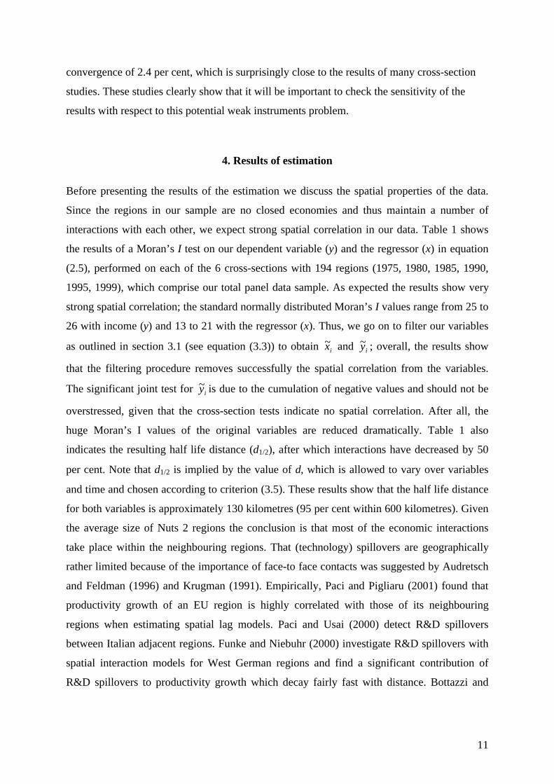
interactions with each other, we expect strong spatial correlation in our data. Table 1 shows

the results of a Moran’s I test on our dependent variable (y) and the regressor (x) in equation

(2.5), performed on each of the 6 cross-sections with 194 regions (1975, 1980, 1985, 1990,

1995, 1999), which comprise our total panel data sample. As expected the results show very

strong spatial correlation; the standard normally distributed Moran’s I values range from 25 to

26 with income (y) and 13 to 21 with the regressor (x). Thus, we go on to filter our variables

as outlined in section 3.1 (see equation (3.3)) to obtain ix~ and iy~ ; overall, the results show

that the filtering procedure removes successfully the spatial correlation from the variables.

The significant joint test for iy~ is due to the cumulation of negative values and should not be

overstressed, given that the cross-section tests indicate no spatial correlation. After all, the

huge Moran’s I values of the original variables are reduced dramatically. Table 1 also

indicates the resulting half life distance (d1/2), after which interactions have decreased by 50

per cent. Note that d1/2 is implied by the value of δ, which is allowed to vary over variables

and time and chosen according to criterion (3.5). These results show that the half life distance

for both variables is approximately 130 kilometres (95 per cent within 600 kilometres). Given

the average size of Nuts 2 regions the conclusion is that most of the economic interactions

take place within the neighbouring regions. That (technology) spillovers are geographically

rather limited because of the importance of face-to face contacts was suggested by Audretsch

and Feldman (1996) and Krugman (1991). Empirically, Paci and Pigliaru (2001) found that

productivity growth of an EU region is highly correlated with those of its neighbouring

regions when estimating spatial lag models. Paci and Usai (2000) detect R&D spillovers

between Italian adjacent regions. Funke and Niebuhr (2000) investigate R&D spillovers with

spatial interaction models for West German regions and find a significant contribution of

R&D spillovers to productivity growth which decay fairly fast with distance. Bottazzi and

12

Peri (1999) regard EU regions and similarly find that local clustering, i.e. spillovers, is

important for R&D results, while R&D spillovers quickly fade with distance.

Table 1 – Test for spatial correlation of the variables in (2.5)

x ix~ y iy~

zI (75) 25.71*** d1/2 = 135 -1.09zI (80) 21.68*** d1/2 = 127 1.24 26.30*** d1/2 = 133 -1.14zI (85) 15.99*** d1/2 = 122 -1.27 24.85*** d1/2 = 133 -1.81*

zI (90) 15.99*** d1/2 = 118 -0.81 23.59*** d1/2 = 136 -1.47

zI (95) 13.32*** d1/2 = 119 -2.01** 26.34*** d1/2 = 133 -1.58

zI (99) 13.66*** d1/2 = 117 1.74* 26.17*** d1/2 = 133 -1.27

zI (joint) 16.13*** -0.22 25.50*** -1.39***

***, **, * indicate significance at the 1, 5 and 10 per cent level. – zI-values are standardised Moran’s I values (seeequation (3.2)), which are assumed to be standard normally distributed under the null of no serial correlation(standardization based on expectation and variance as given in Tiefelsdorf (2000), joint statistic is based onaverage of individual values and is distributed with a mean of zero and a standard deviation of 1/√5 (x),respectively 1/√6 (y). – d1/2 is expressed in kilometres and refers to both the original and the filtered variables.

Tables 2 and 3 present the results of our estimation for equation (2.5) using different

estimators for both the original data and the spaceless models with the filtered variables. Our

sample comprises 194 cross-section units; the data refer to 5 year intervals over the time

period 1975 to 1999.5 A detailed description of the data used in the estimation of (2.5) is

given in the Appendix.

5 As we have no data on the year 2000, the last time period covers only four years. This implies an average τ of4.75, which we use to recover the structural parameters of our model.

13

Table 2 – Results of estimation of model (2.5) (unfiltered variables)

dependent variable: yit

OLS1) LSDV2) GMM-FD3) GMM-SYS4)

constant5) 0.002***

(14.69)5.048 5.614 -0.691

yi,t-1 1.007***

(138.13)0.474***

(13.07)0.353***

(4.44)1.092***

(20.24)

xit 0.035***

(3.05)0.151***

(9.42)0.213***

(6.44)0.321***

(10.37)

implied structural coefficientsλ - 0.157 0.219 -α - 0.223 0.248 -

Instruments diagnostics

Sargan6) 7.76 (4) 27.89*** (8)

Diff-Sargan6) 20.13*** (4)

Moran’s I tests of residuals7)

zI (e85) 5.26*** 12.95*** 13.44*** 5.67***

zI (e90) 11.55*** 4.52*** 5.36*** 9.73***

zI (e95) 6.74*** 11.98*** 16.50*** 14.05***

zI (e99) 21.93*** 16.30*** 15.27*** 19.39***

zI (joint) 11.37*** 11.44*** 12.65*** 12.21***

R2 0.965 0.983 0.960 0.944obs. 776 776 776 970

Numbers in parentheses are t-values, respectively degrees of freedom of the test statistics. – ***, **, * indicatesignificance at the 1, 5 and 10 per cent level. – All models estimated including time-specific effects. – 1) OLS-estimation of pooled data (common intercept) – 2) Least squares dummy variable estimation, based on meancentred data. – 3) two-step GMM estimator, based on first differences (Arellano and Bond 1991); the third andfourth lags (yi,t-3, yi,t-4) were used as instruments for ∆yit (similar as in the case of the levels equations in thesystem estimator, there are no instruments for the first observation; the third lag was chosen because the use oflag two resulted in a significant Sargan test). – 4) two-step GMM system estimator, based on first differences andlevels equations (Blundell and Bond, 1998), the first lagged difference (∆yi,t-1) was used as instruments for yit(starting with lag two leads to no improvement in the Sargan test).– The variable x is treated as exogenous; noimprovement in the Sargan-test is attainable, if x is instrumented, too. – t-statistics refer to two –step estimates;significance levels do not change, if two step or one step robust estimates are used. – 5) constant (in OLS),respectively average of fixed effects µi . – 6) Sargan validity of instruments test: under H0 of valid instrumentsdistributed χ2 with p-k degrees of freedom, where p is the number of columns in the instrument matrix and k isthe number of variables; Differences-Sargan test of the validity of the additional instruments in the levelsequations of the system, calculated as difference between Sargan (system) and Sargan (first differences). – 7)

Moran’s I; see Table 2; half life distances of endogenous variable were used. – R2 calculated as squaredcorrelation between yit and ity . – GMM estimators were calculated using the DPD98 Software for GAUSS(Arellano and Bond 1998).

14

Let us first look at the results, if spatial dependence is not taken into account (table 2). The

coefficient of lagged income varies considerably according to the estimation procedure. The

OLS coefficient is slightly larger than one indicating an absence of convergence. It goes down

to 0.47 with the LSDV (within groups) estimator and still further to 0.35 with the difference

GMM estimator. The coefficient varies in the expected way. The OLS coefficient is expected

to suffer from an upward bias in the presence of fixed effects (Hsiao 1986), the within groups

estimator from a serious downward bias in a dynamic panel (Nickell 1981, Judson et al.

1999). The coefficient of the difference GMM estimator may even be more downward biased

than the LSDV in the case of weak instruments (Bond et al. 2001). A plausible parameter

estimate should lie between the LSDV and the OLS estimate (Bond et al. 2001, Blundell and

Bond 1995), a result which has been obtained by using the system GMM estimator (Yudong

and Weeks 2000, Bond et al. 2001). However, note that in our case we obtain the surprising

result that the coefficient exceeds that of the OLS estimation, which may be due to a

misspecification of the model in the presence of spatial effects and invalid instruments (see

below). The coefficient of net investment is implausibly low with the OLS estimator and

increases with the LSDV and the dynamic panel estimators. The implied capital elasticity

ranges from 0.22 to 0.24.

Looking at the Sargan tests and the Difference Sargan test, we have to note that the

instruments employed with the system GMM estimator are invalid. The test would rather

suggest that the difference GMM estimation operates with correct instruments although there

remain some doubts on their quality, because the coefficient is even below the LSDV

estimate. If the difference GMM was our "preferred" specification, we would conclude from

this estimation that the convergence speed is 21.9 per cent and capital elasticity 0.25.

This convergence coefficient from the first differences GMM estimate is even higher

than the results reported by other panel data convergence studies. With the difference GMM

estimator, Caselli et al. (1996) obtain a convergence rate of 12.9 per cent, Tondl (2001) of 21

per cent, Panizza (2002) of 14.4 per cent. (Also with LSDV our results resemble those of

other studies, for example, de la Fuente (1996) finds a convergence rate of about 10 per cent,

Deininger and Olinto (2000) of 16.3 per cent, Yudong and Weeks (2000) of 19.3 per cent.) If

we did not care about spatial dependence, that would probably be the (unfortunate) end of our

estimation exercise. However, if we look at the Moran´s I statistic of the residuals which

indicates serious spatial correlation, it is evident that the above results are potentially

misleading due to a model misspecification and that we have to take spatial dependencies into

account.

15

Table 3 – Results of estimation of model (2.5) (based on spatially filtered variables)

dependent variable: ity~

OLS1) LSDV2) GMM-FD3) GMM-SYS4)

constant 0.718***

(5.78)6.692 5.614 2.712

1,~

−tiy 0.932***

(71.75)0.305***

(7.80)0.416***

(3.56)0.720***

(13.73)

tix ,~ 0.121***

(8.92)0.156***

(8.47)0.228***

(5.93)0.214***

(8.92)

implied structural coefficientsλ 0.015 0.250 0.184 0.069α 0.640 0.183 0.281 0.433

Instruments diagnostics

Sargan5) 3.85 (4) 11.32 (8)

Diff-Sargan5) 7.48 (4)

Moran’s I tests of residuals6)

zI (e85) -3.21*** -1.19 -1.54 -2.16**

zI (e90) -1.37 -1.22 -1.04 -1.38zI (e95) 0.55 1.93* 3.40*** 3.25***

zI (e99) 2.31** 1.74 1.29 0.39zI (joint) -0.43 0.32 0.53 0.03

R2 0.932 0.941 0.917 0.928obs. 776 776 776 970

Notes: see Table 2 and Table 1 (for Moran’s I). R2 calculated as squared correlation between y and )].~(~[ yyy −+

Therefore we re-estimate model (2.5) with the spatially filtered variables y~ and x~ . The

results are reported in table 3. If we compare the size of the coefficients of lagged income, the

consideration of spatial dependence obviously has a significant impact on convergence. The

coefficients of lagged income change considerably. With OLS it is now below one, the other

estimates follow the expected pattern where the LSDV coefficient is heavily downward

biased. Both the coefficients of the difference GMM and of the system GMM now lie within

the bound given by the OLS and LSDV coefficient. The Sargan test statistics suggest that

both estimators use valid instruments and that the additional instruments of the system GMM

are correct. The difference GMM estimates are close to the LSDV results which is considered

to indicate a weak instruments problem. We therefore give preference to the results from the

16

system GMM specification which indicates a rate of convergence of 6.9 per cent and a capital

elasticity of 0.43. Our results are similar to the coefficients found with these estimators in the

convergence studies of Yudong and Weeks (2000) and Bond et al. (2001), both with respect

to the size of the coefficients and their relative magnitude. In line with these authors, our

findings cast further doubt on the high convergence rates obtained in previous panel data

studies.

The effectiveness of the spatial filtering procedure becomes evident from the Moran´s I

statistics of the new residuals. Spatial correlation has practically disappeared, although there

still seems to be a small rest of spatial correlation for the observation 1995. From this analysis

we can point to two important findings. First, we see that correct treatment of spatial

dependence is essential in regional convergence analyses and that this can be effectively done

with a spatial filter. Using this filter, one can continue to use a dynamic panel data

framework. Second, we have seen how sensitive the results from panel data analysis can be

with respect to the chosen estimator. According to our results we have to reject the extremely

high rates of convergence reported by previous panel data studies. Our estimated convergence

rate of 6.9 per cent gives a more plausible case. This convergence speed corresponds to a half-

life time of 10 years, after which regions would reach their individual steady state income,

which is determined by region specific factors.

5. Conclusions

In this paper, we estimated the speed of convergence for a broad set of EU NUTS 2 level

regions over the period 1985-1999. The objective of this study was to address a major

econometric problem in regional convergence analysis: How to account for spatial effects in a

dynamic panel data model? This estimation problem departs from two important issues. First,

regions are no closed economies but show intensive economic interactions with each other.

Therefore, one has to expect spatial dependence in the observations. Second, making

inference on convergence in a panel data model means that one has to chose a consistent

estimator for a dynamic panel data model. Since there exists no dynamic panel data estimator

which accounts for spatial dependence we propose a two-step procedure, which involves

filtering of the data to remove spatial effects (step 1) and the application of a standard GMM

estimators for dynamic panels (step 2).

17

Our analysis shows that EU regional data at the NUTS 2 level exhibits a large degree of

spatial correlation. Our variables, regional income and investment are highly dependent on

that of other regions as shown by the Moran´s I statistic. Our first regression analysis that

does not account for this fact yields regression residuals with a high degree of spatial

correlation. This indicates that a common model that neglects spatial factors is misspecified

and yields misleading results.

We show that the estimation of our convergence model with the spatially filtered

observations removes successfully spatial correlation and that it changes our results on

convergence substantially. We now found evidence for convergence with all relevant

estimators as opposed to the model with the unfiltered data. The parameter estimates with

different panel data estimators now lie within a range and in relationship as proposed by panel

data econometrics.

As several recent studies in the empirical growth literature, we found that the system

GMM estimator performs best. With this estimator we obtain a convergence speed of about 7

per cent and an output elasticity of capital of 0.4. This indicates a more modest and more

plausible convergence process than proposed by previous panel data convergence analyses for

EU regions.

18

References

Anselin, L. (1988), Spatial econometrics: Methods and models, Dordrecht, Kluwer AcademicPublishers.

Anselin, L. and Bera, A. (1998), Spatial dependence in linear regression models with anintroduction to spatial econometrics, in Giles, D., Ullah, A. (eds.) Handbook ofapplied economic statistics, New York: Marcel Dekker, pp. 237-289.

Anselin, L. and Florax, J. (1995), New directions in spatial econometrics: Introduction, in:Anselin, L. and Florax, J. (eds.), New directions in spatial econometrics,Berlin/Heidelberg /New York, Springer.

Arellano, M. and Bover, S. (1995), Another look at the instrumental variable estimation oferror-component models, Journal of Econometrics, 68, pp. 29-52.

Arellano, M. and Bond, S. (1991), Some tests of specification for panel data: Monte Carloevidence and an application to employment equations, Review of Economic Studies,58, pp. 277-297.

Arellano, M., and Bond, S. (1998), Dynamic panel data estimation using DPD98 for GAUSS:a guide for users, mimeo, Institute for Fiscal Studies, London.

Armstrong, H. (1995), Convergence among regions of the European Union, 1950-1990,Papers in Regional Science, 74(2) , pp. 143-52.

Baltagi, B.H. (1995), Econometric analysis of panel data, Chichester, Wiley.Barro, R. (1991), Economic growth in a cross-section of countries, The Quarterly Journal of

Economics, May 1991, pp. 407-43.Barro, R. and Sala-i-Martin, X. (1991), Convergence across states and regions, Brookings

Papers on Economic Activity, no. 1 / 1991, pp. 107-182.Baumol, C., Ertur, C. and Le Gallo, J. (2002), Spatial Convergence Clubs and the European

Growth Process, 1980-1995, in: Fingleton, B. (ed.), European regional growth,Advances in Spatial Science, Berlin et al., Springer (forthcoming).

Blundell, R. and Bond, S. (1998), Initial conditions and moment restrictions in dynamic paneldata models, Econometrica, 87(1), pp. 115-143.

Blundell, R. and Bond, S. (1998), Initial conditions and moment restrictions in dynamic paneldata models, Journal of Econometrics, 87(1), pp. 115-143.

Blundell, R., Bond, S. and Windmeijer F. (2000), Estimation in dynamic panel data models:Improving the perfomance of the standard GMM estimator, in: Baltagi B. (ed.),Nonstationary panels, panel cointegration, and dynamic panels. Advances inEconometrics, vol. 15, Amsterdam et al., Elsevier Science.

Bond, S., Hoeffler, A. and Temple, J. (2001), GMM estimation of empirical growth models,CEPR discussion paper no. 3048, Centre for Economic Policy Research, London.

Bröcker, J. (1989), Determinanten regionalen Wachstums im sekundären und tertiären Sektorder Bundesrepublik Deutschland 1970 bis 1982. Schriften des Instituts fürRegionalforschung der Universität Kiel, vol. 10, München, Florentz.

Carrington, A. (2002), A divided Europe? Regional convergence and neighbourhood spillovereffects, Bradford University, mimeo.

Caselli,F., Esquivel,G. and Lefort, F. (1996), Reopening the convergence debate: A new lookat cross-country growth empirics, Journal of Economic Growth; 1(3), pp. 363-89.

19

Cuadrado-Roura, J., Garcia-Greciano, B., Raymond, J.(1999), Regional convergence inproductivity and productive structure: The Spanish case, International RegionalScience Review; 22(1), pp. 35-53.

de la Fuente, A. (1996), On the sources of convergence: A close look at the Spanish regions,CEPR discussion paper no. 1543, Centre for Economic Policy Research, London.

Deininger, K., Olinto, P. (2000), Asset distribution, inequality, and growth, World Bankworking paper no. 2375, The World Bank, Washington.

Dowrick, S. and Rogers, M. (2001), Classical and technological convergence: Beyond theSolow-Swan model, Australian National University.

Fagerberg, J.and Verspagen, B. (1996), Heading for divergence? Regional growth in Europereconsidered, Journal of Common Market Studies, 34(3), September 1996, pp. 431-48.

Fingleton, B. (1999), Estimates of time to economic convergence: An analysis of regions ofthe European Union, International Regional Science Review, 22, pp. 5-34.

Fingleton, B. and McCombie, J. (1998), Increasing returns and economic growth: Someevidence for manufacturing from European Union regions, Oxford Economic Papers,50, pp. 89-105.

Getis, A. (1995), Spatial filtering in a regression framework: Experiments on regionalinequality, government expenditures, and urban crime,” in: Anselin, L. and Florax,R.J.G.M. (eds.), New Directions in Spatial Econometrics, Berlin, Springer, pp. 172-188.

Getis, A., and Griffith, D.A. (2002), Comparative spatial filtering in regression analysis,Geographical Analysis, 34(2), pp. 130-140.

Getis, A., and Ord, J.K. (1992), The Analysis of Spatial Association by Use of DistanceStatistics, Geographical Analysis, 24, pp. 189-206.

Henderson, V. (2000), The effects of urban concentration on economic growth, NBERworking paper 7503, National Bureau of Economic Research, Cambridge, MA.

Herz, B. and Röger, W. (1995), Economic growth and convergence in Germany,Weltwirtschaftliches Archiv, no.1/1995, pp. 133-143.

Hofer, H. and Wörgötter, A. (1997), Regional per capita income convergence in Austria,Regional Studies, 31(1), pp. 1-12.

Hsiao, C. (1986) Analysis of Panel Data. Cambridge: Cambridge University Press.Islam, N. (1995), Growth empirics: A panel data approach, Quarterly Journal of Economics,

110(4), pp. 1127-1170.Kelejian, H., and Prucha, I.R. (1999), A generalized moments estimator for the autoregressive

parameter in a spatial model, International Economic Review, 40, pp. 509-533.Kelejian, H. and Prucha, I., (1998), A generalized spatial two-stage least squares procedure

for estimating a spatial autoregressive model with autoregressive disturbances,Journal of Real Estate Finance and Economics, pp. 99-121.

Knight, M., Loayza, N. and Villanueva D. (1993), Testing the neoclassical theory ofeconomic growth: A panel data approach, IMF Staff Papers no. 40, InternationalMonetary Fund, Washington.

Levine, R. and Renelt, D. (1992), A sensitivity analysis of cross-country growth regressions,American Economic Review, 82(4), September 1992, pp. 942-963.

20

Mankiw, G., Romer, D. and Weil, D. (1992), A contribution to the empirics of economicgrowth, Quarterly Journal of Economics, 111(3), pp. 407-434.

Martin, Reiner (1999), Regional convergence in the EU: Determinants for catching-up orstaying behind, Jahrbuch –für Regionalwissenschaft, 19(2), 1999, pp. 157-81.

Martin, Ron (2000), EMU versus the regions? Regional convergence and divergence inEuroland, University of Cambridge, ESRC Centre for Business Research WorkingPaper: WP179, September 2000.

Neven, D., Gouyette, C.(1995), Regional convergence in the European Community, Journalof Common Market Studies, 33(1), March 1995, pp. 47-65.

Nickell, S. (1981), Biases in dynamic models with fixed effects, Econometrica, 49, pp. 1417–1426.

Niebuhr, A. (2001), Convergence and the effects of spatial interaction, Jahrbuch fürRegionalwissenschaft, 21, pp. 113-133.

Ord, J.K., and Getis, A. (1995), Local spatial autocorrelation statistics: Distributional issuesand an application, Geographical Analysis, 27(4), pp. 286-305.

Paci, R. and Pigliaru, F. (1995), Differenziali di crescita tra le regioni italiane: Un´analisicross-section, Rivista di Politica Economia, 85, October 1995, pp. 3-34.

Panizza, U. (2002), Income inequality and economic growth: Evidence from American data,Journal of Economic Growth, 7, pp. 25-41.

Quah, D. (1996), Regional convergence clusters across Europe. European Economic Review,40, pp. 951-958.

Rey, S., Montouri B. (1999), US regional income convergence: A spatial econometricperspective, Regional Studies, 33, pp. 143-156.

Tiefelsdorf, M. (2000), Modelling Spatial Processes, Springer Lecture Notes in EarthSciences, Berlin: Springer Verlag.Tondl G. (2001), Convergence after divergence?Regional growth in Europe, Springer, Wien/Heidelberg/New York.

Tondl, G. (1999), The changing pattern of regional convergence in Europe, Jahrbuch fürRegionalwissenschaft, 19(1), pp. 1-33.

Tondl, G. (2001), Convergence after divergence? Regional growth in Europe, Springer,Wien/Heidelberg/New York.

Vanhoudt, P., Matha, T. and Smid, B. (2000), How productive are capital investments inEurope?, EIB-Papers, 5(2), pp. 81-106.

Vayá, E., López-Bazo, E., Moreno, R. and Surinach, J. (2000), Growth and externalitiesacross economies. An empirical analysis using spatial econometrics, Working PaperEconomic and Social Sciences no. EOO/59, University of Barcelona.

Yudong, Y. and Weeks, M. (2000), Provicial income convergence in China, 1953-1997: Apanel data approach, DAE working paper 0010, University of Cambridge, October2000.

21

Appendix

Data

ityln = GVA/POP gross value added per capita in million ECU at time t (1990 prices, 1990exchange rate) (t = 1, ..., 6).

its = investment-ratio = INVit/GVAit, average of the (five year) period (t = 2, ..., 6).

nit = growth of population over the (5 year) period t to t-1, calculated as differences in naturallogs (t = 2, ..., 6).

git = growth of technological progress, κ it = depreciation rate of capital stock; )( κ+g isassumed to be equal to 25 per cent for all regions over the 5 year period t to t-1 (t = 2, ..., 6).

INVit = investment expenditures (including public investment) in million ECU (1990 prices,1990 exchange rate)

GVAit = gross value added in million ECU (1990 prices, 1990 exchange rate)

POPit = population in 1000 persons.

i = 1, . . . , 194 European regions (all NUTS2 regions of the EU-15 countries as available inthe Cambridge Econometrics dataset, part of the regions had to be eliminated due to missingdata or because they turned out as obvious ouliers****), t = 1, . . . , 6 (1975, 1980, 1985,1990, 1995, 1999). All data were taken from the Cambridge Econometrics Dataset (2001).Distances between capitals of the NUTS2 districts were kindly provided by Eurostat.

original data set: 212 regions (Cambridge econometrics)**** of the originally 212 regions we had to exclude the following 18 regions:BE34 LuxembourgDE4 BrandenburgDE8 Mecklenburg-Vorpomm.DED1 ChemnitzDED2 DresdenDED3 LeipzigDEE1 DessauDEE2 HalleDEE3 MagdeburgDEG ThuringenES63 Ceuta y MelillaFR91 GuadeloupeFR92 MartiniqueFR93 GuyaneFR94 ReunionPT15 AlgarvePT2 AcoresPT3 Madeira

22

INCLUDED REGIONS (194)AT11 Burgenland GR11 Anat.Mak.AT12 Niederosterreich GR12 Kent. Makedonia.AT13 Wien GR13 Dytiki MakedoniaAT21 Karnten GR14 ThessaliaAT22 Steiermark GR21 IpeirosAT31 Oberosterreich GR22 Ionia NisiaAT32 Salzburg GR23 Dytiki ElladaAT33 Tirol GR24 Sterea ElladaAT34 Vorarlberg GR25 PeloponnisosBE1 Bruxelles-Brussel GR3 AttikiBE21 Antwerpen GR41 Voreio AigaioBE22 Limburg GR42 Notio AigaioBE23 Oost-Vlaanderen GR43 KritiBE24 Vlaams Brabant IE01 BorderBE25 West-Vlaanderen IE02 Southern and EasternBE31 Brabant Wallon IT11 PiemonteBE32 Hainaut IT12 Valle d'AostaBE33 Liege IT13 LiguriaBE35 Namur IT2 LombardiaDE11 Stuttgart IT31 Trentino-Alto AdigeDE12 Karlsruhe IT32 VenetoDE13 Freiburg IT33 Fr.-Venezia GiuliaDE14 Tubingen IT4 Emilia-RomagnaDE21 Oberbayern IT51 ToscanaDE22 Niederbayern IT52 UmbriaDE23 Oberpfalz IT53 MarcheDE24 Oberfranken IT6 LazioDE25 Mittelfranken IT71 AbruzziDE26 Unterfranken IT72 MoliseDE27 Schwaben IT8 CampaniaDE3 Berlin IT91 PugliaDE5 Bremen IT92 BasilicataDE6 Hamburg IT93 CalabriaDE71 Darmstadt ITA SiciliaDE72 Giessen ITB SardegnaDE73 Kassel NL11 GroningenDE91 Braunschweig NL12 FrieslandDE92 Hannover NL13 DrentheDE93 Luneburg NL21 OverijsselDE94 Weser-Ems NL22 GelderlandDEA1 Dusseldorf NL23 FlevolandDEA2 Koln NL31 UtrechtDEA3 Munster NL32 Noord-HollandDEA4 Detmold NL33 Zuid-HollandDEA5 Arnsberg NL34 ZeelandDEB1 Koblenz NL41 Noord-BrabantDEB2 Trier NL42 LimburgDEB3 Rheinhessen-Pfalz PT11 NorteDEC Saarland PT12 CentroDEF Schleswig-Holstein PT13 Lisboa e V.do TejoDK01 Hovedstadsreg. PT14 AlentejoDK02 O. for Storebaelt PT15 AlgarveDK03 V. for Storebaelt SE01 StockholmES11 Galicia SE02 Ostra Mellansverige

23

ES12 Asturias SE04 SydsverigeES13 Cantabria SE06 Norra MellansverigeES21 Pais Vasco SE07 Mellersta NorrlandES22 Navarra SE08 Ovre NorrlandES23 Rioja SE09 Smaland med oarnaES24 Aragon SE0A VastsverigeES3 Madrid UKC1 Tees Valley and DurhamES41 Castilla-Leon UKC2 Northumb. et al.ES42 Castilla-la Mancha UKD1 CumbriaES43 Extremadura UKD2 CheshireES51 Cataluna UKD3 Greater ManchesterES52 Com. Valenciana UKD4 LancashireES53 Baleares UKD5 MerseysideES61 Andalucia UKE1 East RidingES62 Murcia UKE2 North YorkshireFI13 Ita-Suomi UKE3 South YorkshireFI14 Vali-Suomi UKE4 West YorkshireFI15 Pohjois-Suomi UKF1 DerbyshireFI16 Uusimaa UKF2 Leics.FI17 Etela-Suomi UKF3 LincolnshireFI2 Aland UKG1 Hereford et al.FR1 Ile de France UKG2 Shrops.FR21 Champagne-Ard. UKG3 West Midlands (county)FR22 Picardie UKH1 East AngliaFR23 Haute-Normandie UKH2 BedfordshireFR24 Centre UKH3 EssexFR25 Basse-Normandie UKI1 Inner LondonFR26 Bourgogne UKI2 Outer LondonFR3 Nord-Pas de Calais UKJ1 Berkshire et al.FR41 Lorraine UKJ2 SurreyFR42 Alsace UKJ3 Hants.FR43 Franche-Comte UKJ4 KentFR51 Pays de la Loire UKK1 Avon et al.FR52 Bretagne UKK2 DorsetFR53 Poitou-Charentes UKK3 CornwallFR61 Aquitaine UKK4 DevonFR62 Midi-Pyrenees UKL1 West WalesFR63 Limousin UKL2 East WalesFR71 Rhone-Alpes UKM1 North East Scot.FR72 Auvergne UKM2 Eastern ScotlandFR81 Languedoc-Rouss. UKM3 South West Scot.FR82 Prov-Alpes-Cote d'Azur UKM4 Highlands and IslandsFR83 Corse UKN Northern Ireland

24

Bisher erschienene IEF Working Papers

1 Gerhard Fink, A Schedule of Hope for the New Europe, Oktober 1993.2 Gerhard Fink, Jutta Gumpold, Österreichische Beihilfen im europäischen

Wirtschaftsraum (EWR), Oktober 1993.3 Gerhard Fink, Microeconomic Issues of Integration, November 1993.4 Fritz Breuss, Herausforderungen für die österreichische Wirtschaftspolitik und

die Sozialpartnerschaft in der Wirtschafts- und Währungsunion, November1993.

5 Gerhard Fink, Alexander Petsche, Central European Economic Policy Issues,July 1994.

6 Gerhard Fink, Alexander Petsche, Antidumping in Österreich vor und nach derOstöffnung, November 1994.

7 Fritz Breuss, Karl Steininger, Reducing the Greenhouse Effect in Austria: AGeneral Equilibrium Evaluation of CO2-Policy-Options, March 1995.

8 Franz-Lothar Altmann, Wladimir Andreff, Gerhard Fink, Future Expansion ofthe European Union in Central Europe, April 1995.

9 Gabriele Tondl, Can EU's Cohesion Policy Achieve Convergence?, April 1995.10 Jutta Gumpold, Nationale bzw. gesamtwirtschaftliche Effekte von Beihilfen -

insbesondere Exportbeihilfen, April 1995.11 Gerhard Fink, Martin Oppitz, Kostensenkungspotentiale der Wiener Wirtschaft

- Skalenerträge und Kostendruck, August 1995.12 Alexander Petsche, Die Verfassung Ungarns im Lichte eines EU-Beitritts,

September 1995.13 Michael Sikora, Die Europäische Union im Internet, September 1995.14 Fritz Breuss, Jean Tesche, A General Equilibrium Analysis of East-West Mi-

gration: The Case of Austria-Hungary, January 1996.15 Alexander Petsche, Integrationsentwicklung und Europaabkommen EU -

Ungarn, Juli 1996.16 Jutta Gumpold, Die Ausfuhrförderung in der EU, Juni 1996.17 Jutta Gumpold, Internationale Rahmenregelungen zur Ausfuhrförderung, Juni

1996.18 Fritz Breuss, Austria's Approach towards the European Union, April 1996.19 Gabriele Tondl, Neue Impulse für die österreichische Regionalpolitik durch die

EU-Strukturfonds, Mai 1996.20 Griller, Droutsas, Falkner, Forgó, Klatzer, Mayer, Nentwich, Regierungskon-

ferenz 1996: Ausgangspositionen, Juni 1996.21 Stefan Griller, Ein Staat ohne Volk? Zur Zukunft der Europäischen Union,

Oktober 1996.22 Michael Sikora, Der „EU-Info-Broker“ – ein datenbankgestütztes Europa-

informationssystem im World Wide Web über die KMU-Förderprogramme derEuropäischen Kommission, November 1996.

23 Katrin Forgó, Differenzierte Integration, November 1996.24 Alexander Petsche, Die Kosten eines Beitritts Ungarns zur Europäischen Union,

Januar 1997.

25

25 Stefan Griller, Dimitri Droutsas, Gerda Falkner, Katrin Forgó, MichaelNentwich, Regierungskonferenz 1996: Der Vertragsentwurf der irischenPräsidentschaft, Januar 1997.

26 Dimitri Droutsas, Die Gemeinsame Außen- und Sicherheitspolitik derEuropäischen Union. Unter besonderer Berücksichtigung der NeutralitätÖsterreichs, Juli 1997.

27 Griller, Droutsas, Falkner, Forgó, Nentwich, Regierungskonferenz 1996: DerVertrag von Amsterdam in der Fassung des Gipfels vom Juni 1997, Juli 1997.

28 Michael Nentwich, Gerda Falkner, The Treaty of Amsterdam. Towards a NewInstitutional Balance, September 1997.

29 Fritz Breuss, Sustainability of the Fiscal Criteria in Stage III of the EMU,August 1998.

30 Gabriele Tondl, What determined the uneven growth of Europe´s Southernregions? An empirical study with panel data, März 1999.

31 Gerhard Fink, New Protectionism in Central Europe - Exchange RateAdjustment, Customs Tariffs and Non-Tariff Measures, Mai 1999.

32 Gerhard Fink, Peter Haiss, Central European Financial Markets from an EUPerspective. Review of the Commission (1998) Progress Report onEnlargement, Juni 1999.

33 Fritz Breuss, Costs and Benefits of EU Enlargement in Model Simulations, Juni1999.

34 Gerhard Fink, Peter R. Haiss, Central European Financial Markets from an EUPerspective. Theoretical aspects and statitical analyses, August 1999.

35 Fritz Breuss, Mikulas Luptacik, Bernhard Mahlberg, How far away are theCEECs from the EU economic standards? A Data Envelopement Analysis ofthe economic performance of the CEECs, Oktober 2000.

36 Katrin Forgó, Die Internationale Energieagentur. Grundlagen und aktuelleFragen, Dezember 2000

37 Harald Badinger, The Demand for International Reserves in the Eurosystem,Implications of the Changeover to the Third Stage of EMU, Dezember 2000.

38 Harald Badinger, Fritz Breuss, Bernhard Mahlberg, Welfare Implications ofthe EU’s Common Organsiation of the Market in Bananas for EU MemberStates, April 2001

39 Fritz Breuss, WTO Dispute Settlement from an Economic Perspective – MoreFailure than Success, Oktober 2001.

40 Harald Badinger, Growth Effects of Economic Integration – The Case of theEU Member States, Dezember 2001.

41 Gerhard Fink, Wolfgang Koller, Die Kreditwürdigkeit von Unternehmen imHinblick auf die Wirtschafts- und Währungsunion - Wien im österreichischenVergleich, Dezember 2001.

42 Harald Badinger, Gabriele Tondl, Trade, Human Capital and Innovation: TheEngines of European Regional Growth in the 1990s, Januar 2002.

43 David Blum, Klaus Federmair, Gerhard Fink, Peter Haiss, The Financial-RealSector Nexus: Theory and Empirical Evidence, September 2002.

44 Harald Badinger, Barbara Dutzler, Excess Reserves in the Euroystem: AnEconomic and Legal Analysis, September 2002.

26

45 Gerhard Fink, Nigel Holden, Collective Culture Shock: Constrastive Reactionsto Radical Systemic Change, Oktober 2002.

46 Harald Badinger, Fritz Breuss, Do small countries of a trade bloc gain more ofits enlargement? An empirical test of the Casella effect for the case of theEuropean Community, Oktober 2002.

27

Bisher erschienene Bände der Schriftenreihe desForschungsinstituts für Europafragen

(Zu beziehen über den Buchhandel)

1 Österreichisches Wirtschaftsrecht und das Recht der EG. Hrsg von Karl Kori-nek/Heinz Peter Rill. Wien 1990, Verlag Orac. XXIV und 416 Seiten. (öS 1.290,-)

2 Österreichisches Arbeitsrecht und das Recht der EG. Hrsg von Ulrich Rung-galdier. Wien 1990, Verlag Orac. XIII und 492 Seiten. (öS 1.290,-)

3 Europäische Integration aus österreichischer Sicht. Wirtschafts-, sozial undrechtswissenschaftliche Aspekte. Hrsg von Stefan Griller/Eva Lavric/ReinhardNeck. Wien 1991, Verlag Orac. XXIX und 477 Seiten. (öS 796,-)

4 Europäischer Binnenmarkt und österreichisches Wirtschaftsverwaltungsrecht. Hrsgvon Heinz Peter Rill/Stefan Griller. Wien 1991, Verlag Orac. XXIX und 455Seiten. (öS 760,-)

5 Binnenmarkteffekte. Stand und Defizite der österreichischen Integrationsfor-schung. Von Stefan Griller/Alexander Egger/Martina Huber/Gabriele Tondl. Wien1991, Verlag Orac. XXII und 477 Seiten. (öS 796,-)

6 Nationale Vermarktungsregelungen und freier Warenverkehr. Untersuchung derArt. 30, 36 EWG-Vertrag mit einem Vergleich zu den Art. 13, 20Freihandelsabkommen EWG - Österreich. Von Florian Gibitz. Wien 1991, VerlagOrac. XIV und 333 Seiten. (öS 550,-)

7 Banken im Binnenmarkt. Hrsg von Stefan Griller. Wien 1992, Service Fach-verlag. XLII und 1634 Seiten. (öS 1.680,-)

8 Auf dem Weg zur europäischen Wirtschafts- und Währungsunion? Das Für undWider der Vereinbarungen von Maastricht. Hrsg von Stefan Griller. Wien 1993,Service Fachverlag. XVII und 269 Seiten. (öS 440,-)

9 Die Kulturpolitik der EG. Welche Spielräume bleiben für die nationale, insbe-sondere die österreichische Kulturpolitik? Von Stefan Griller. Wien 1995, ServiceFachverlag.

10 Das Lebensmittelrecht der Europäischen Union. Entstehung, Rechtsprechung,Sekundärrecht, nationale Handlungsspielräume. Von Michael Nentwich. Wien1994, Service Fachverlag. XII und 403 Seiten. (öS 593,-)

11 Privatrechtsverhältnisse und EU-Recht. Die horizontale Wirkung nicht umge-setzten EU-Rechts. Von Andreas Zahradnik. Wien 1995, Service Fachverlag. (öS345,-)

12 The World Economy after the Uruguay Round. Hrsg von Fritz Breuss. Wien 1995,Service Fachverlag. XVII und 415 Seiten. (öS 540,-)

13 European Union: Democratic Perspectives after 1996. Von Gerda Falkner/Michael Nentwich. Wien 1995, Service Fachverlag. XII und 153 Seiten. (öS 385,-)

14 Rechtsfragen der Wirtschafts- und Währungsunion. Hrsg von Heinz Peter Rill undStefan Griller. Wien 1997, Springer Verlag Wien/New York, 197 Seiten.

15 The Treaty of Amsterdam – Facts Analysis, Prospects. Von Stefan Griller, DimitriP. Droutsas, Gerda Falkner, Katrin Forgó, Michael Nentwich. Wien 2000,Springer Verlag Wien/New York, 643 Seiten.

28

16 Europäisches Umweltzeichen und Welthandel. Grundlagen,Entscheidungsprozesse, rechtliche Fragen. Von Katrin Forgó. Wien 1999, SpringerVerlag Wien/New York 1999, 312 Seiten.

17 Interkulturelles Management. Österreichische Perspektiven. Von Gerhard Fink,Sylvia Meierewert (Hrsg.), Springer Verlag Wien/New York, 2001, 346 Seiten

18 Staatshaftung wegen Gemeinschaftsrechtsverletzung: Anspruchsgrundlage undmaterielle Voraussetzungen. Zugleich ein Beitrag zur Gemeinschaftshaftung, VonBirgit Schoißwohl, Springer Verlag Wien/New York, 2002, 512 Seiten.

19 The Bananana Dispute: A Comprehensive Legal Analysis supplemented by anEconomic Analysis of Welfare Effects. Von Fritz Breuss, Stefan Griller, ErichVranes (Hrsg.), ca 300 Seiten (erscheint demnächst, 2002).

20 External Economic Relations and Foreign Policy in the European Union, VonStefan Griller, Birgit Weidel (Hrsg.), Springer Verlag Wien/New York, 2002, 500Seiten.