The European Journal of Comparative Economics Vol. 2, n. 2, 2005, pp. 177-202 ISSN 1824-2979 Available online at http://eaces.liuc.it Reforms and Economic Growth in Transition Economies: Complementarity, Sequencing and Speed Karsten Staehr 1 University of Tartu Abstract This paper considers the effects of sequencing and reform speed on output performance in transition countries. These largely unsettled issues are addressed using principal component techniques to construct reform clusters and by explicit tests of speed effects. The results indicate that broad-based reforms are good for output growth, but so is a policy of liberalisation and small-scale privatisation without structural reforms. Conversely, large-scale privatisation without adjoining reforms, market opening without supporting reforms and bank liberalisation without enterprise restructuring affect growth negatively. Swift reform policies allow transition countries to benefit from higher growth for longer time. The speed of reforms appears otherwise to have little effect on growth in the short and medium term. JEL Classification: P21, P30, C33, H11 Keywords: Economic reforms, growth, principal components, gradualism versus big-bang 1. Introduction A defining theme in transition economics is Adam Smith’s centuries old question: How do countries become rich? From the start of reforms in the early 1990s, the most important policy objective in the transition countries was to raise living standards by boosting output. The debate over the choice of reform strategy was fuelled by the deep production falls experienced in all transition economies. Adam Smith’s question essentially epitomises the discussion of which reform strategy is most likely to be successful. Case studies provide valuable insights into the effects of reforms on short-term growth and other variables of interest. 2 They allow a detailed analysis of reforms, taking into account political and socio-economic factors. Unfortunately, case studies do not necessarily produce results that can be broadly generalised and their conclusions may be influenced unduly by recent experience. 3 The most important approach to analysing the effects of reforms on output growth is cross-section or panel data estimations, explaining the short-term output 1 University of Tartu, Lossi 3-319, 51003 Tartu, Estonia. E-mail: [email protected]. I would like to thank editors Michael Keren and Vittorio Valli and an anonymous referee of the European Journal of Comparative Economics for helpful comments and suggestions. I am also grateful for feedback from Abdur Chowdury, Balazs Egert, Tuuli Koivu, Iikka Korhonen, Jukka Pirttila and Jouko Rautava as well as seminar participants at BOFIT, the Central Bank of Norway and University of Tartu. 2 See Campos and Coricelli (2002) footnote 47 for a listing of case studies considering the impact of reforms on growth and other economic variables. IMF Article IV consultations and the OECD Economic Surveys routinely discuss country performance in the light of reforms undertaken and point out areas of “unfinished reforms” that may impede growth. 3 The assessment of the large-scale voucher privatisation in the Czech Republic illustrates this point. The method was initially considered highly successful as the Czech economy boomed in the mid-1990s, but later discredited following the country’s poor performance in the late 1990s.

Welcome message from author
This document is posted to help you gain knowledge. Please leave a comment to let me know what you think about it! Share it to your friends and learn new things together.
Transcript
The European Journal of Comparative Economics Vol 2 n 2 2005 pp 177-202
ISSN 1824-2979
Available online at httpeacesliucit
Reforms and Economic Growth in Transition Economies Complementarity Sequencing and Speed
Karsten Staehr1 University of Tartu
Abstract
This paper considers the effects of sequencing and reform speed on output performance in transition countries These largely unsettled issues are addressed using principal component techniques to construct reform clusters and by explicit tests of speed effects The results indicate that broad-based reforms are good for output growth but so is a policy of liberalisation and small-scale privatisation without structural reforms Conversely large-scale privatisation without adjoining reforms market opening without supporting reforms and bank liberalisation without enterprise restructuring affect growth negatively Swift reform policies allow transition countries to benefit from higher growth for longer time The speed of reforms appears otherwise to have little effect on growth in the short and medium term
JEL Classification P21 P30 C33 H11
Keywords Economic reforms growth principal components gradualism versus big-bang
1 Introduction
A defining theme in transition economics is Adam Smithrsquos centuries old question How do countries become rich From the start of reforms in the early 1990s the most important policy objective in the transition countries was to raise living standards by boosting output The debate over the choice of reform strategy was fuelled by the deep production falls experienced in all transition economies Adam Smithrsquos question essentially epitomises the discussion of which reform strategy is most likely to be successful
Case studies provide valuable insights into the effects of reforms on short-term growth and other variables of interest2 They allow a detailed analysis of reforms taking into account political and socio-economic factors Unfortunately case studies do not necessarily produce results that can be broadly generalised and their conclusions may be influenced unduly by recent experience3
The most important approach to analysing the effects of reforms on output growth is cross-section or panel data estimations explaining the short-term output
1 University of Tartu Lossi 3-319 51003 Tartu Estonia E-mail karstenstaehrutee I would like to
thank editors Michael Keren and Vittorio Valli and an anonymous referee of the European Journal of Comparative Economics for helpful comments and suggestions I am also grateful for feedback from Abdur Chowdury Balazs Egert Tuuli Koivu Iikka Korhonen Jukka Pirttila and Jouko Rautava as well as seminar participants at BOFIT the Central Bank of Norway and University of Tartu
2 See Campos and Coricelli (2002) footnote 47 for a listing of case studies considering the impact of reforms on growth and other economic variables IMF Article IV consultations and the OECD Economic Surveys routinely discuss country performance in the light of reforms undertaken and point out areas of ldquounfinished reformsrdquo that may impede growth
3 The assessment of the large-scale voucher privatisation in the Czech Republic illustrates this point The method was initially considered highly successful as the Czech economy boomed in the mid-1990s but later discredited following the countryrsquos poor performance in the late 1990s
178
EJCE vol 2 n 2 (2005)
Available online at httpeacesliucit
growth by variables reflecting economic reforms while controlling for other factors The first contributions appearing in the mid-1990s were the starting point for an extensive literature Nevertheless a number of issues related to the choice of reform strategy and its impact on growth remain largely unresolved in particular
bull What is the relative importance of individual reform elements bull Can different reform elements substitute for each other or are some reforms
complementary in the sense that their implementation has to be synchronised or sequenced to obtain favourable results
bull How rapidly should reforms be implemented The lack of firm empirical evidence on these questions is unfortunate as it
hampers the ex post evaluation of the different reform strategies carried out in the transition countries Moreover policymakers in all transition countries continue to face sequencing and speed issues when designing reform packages (Nsouli et al 2002)
The questions also take centre place in the occasionally heated debate on reform strategy eg World Bank (1996) and Stiglitz (2001)4 Two camps have emerged One camp ndash under labels like ldquobig-bangrdquo ldquocold turkeyrdquo or ldquomarket fundamentalismrdquo ndash favours rapid and comprehensive reforms The basic premise is that reforms should progress as fast and on as many fronts as possible because various reform elements can (at least to some extent) substitute for each other The other camp ndash under labels like ldquogradualismrdquo or ldquoevolutionary-institutionalist perspectiverdquo ndashemphasises timing and sequencing of specific reforms and tends to favour slower implementation of reforms Complementarities between specific sets of reforms are seen as important so reforms must be sequenced ie certain reforms are prerequisites to other reforms
We seek within the framework of growth regressions to make progress on the three contentious issues above5 First we apply principal component analysis on (stacked) reform indices to identify ldquoreform clustersrdquo This allows a deeper discussion of the overall design of reform programs in transition economies Second we address inference problems stemming from the correlation of many reform variables This facilitates identification of which reforms are most important for economic growth Third we use estimation with reform clusters as right-hand side variables to reveal complementarities between reform elements This provides insight into the reform sequencing issue Fourth the importance of speed is addressed in considerable detail Several direct tests are devised and implemented
This paper uses the term output growth in the same way as most other papers in this literature viz as the annual change in output during the period transition In the nature of the case long-term changes in output cannot be analysed for the transition economies as the transition process started in the early 1990s
The paper is organised as follows Section 2 reviews the literature of growth estimations for transition economies Section 3 discusses selection of an econometric
4 Wolf (1999) and Roland (2001) survey the debate the latter with an emphasis on political economy
arguments See also IMF (2000) for an overview and references The debate is based on different assessments of how both transition and market economies function The approaches have divergent views on the political economy of reform in particular the conditions for maintaining reform momentum There are also different perspectives on the amount of uncertainty linked to reforms and how to manage this uncertainty It is essentially an empirical problem to evaluate which reform strategy ndash including choice of specific reforms sequencing and speed ndash yields the best results
5 Note that the discussion on reform strategy raises many issues besides growth effects These include distribution political consolidation and long-term sustainability
Karsten Staehr Reforms and Economic Growth in Transition Economies
Available online at httpeacesliucit
179
model and variables Section 4 analyses the correlation pattern of reform variables and derives reform clusters Section 5 estimates the impact of reform clusters and control variables on growth Section 6 tests how reform speed affects growth Section 7 concludes
2 Growth regressions for transition economies
The literature on growth regressions for transition economies seeks to explain the countriesrsquo short-term growth performance by miscellaneous variables that reflect eg economic reforms initial conditions or economic shocks A diverse range of variables has been employed for right-hand side variables while variables accounting for accumulation of human and physical capital are typically omitted6 This approach owes its intellectual debt to the ldquonew growthrdquo literature of the 1990s (Havrylyshyn et al 1998)
Fischer et al (1996a) initiated the literature Their analysis used a panel of annual data 1992-94 for 25 transition economies Monetary stabilisation as captured by budget balance and an exchange rate regime dummy were positively linked with growth7 Transition reforms were measured by a ldquocumulative liberalisation indexrdquo which weighted scores for price liberalisation trade liberalisation privatisation and banking reform each year calculated by accumulating the scores for all previous years of reform8 The cumulative liberalisation index also proved beneficial to growth
Fischer et al (1996a) has been succeeded by a host of papers estimating growth regressions for transition economies The papers are too numerous to cite but survey papers have recently synthesised the literature Havrylyshyn (2001) focuses entirely on growth regressions while Fischer and Sahay (2000) Campos and Coricelli (2002) World Bank (2002) and EBRD (2004 ch 1) frame the results from regression analyses in broader discussions9 The survey papers generally agree on the following
bull All transition economies experienced an initial steep fall in production even
those undertaking very limited reforms Clearly reforms cannot explain the output drop
bull Traditional factor analysis plays no role in explaining the growth performance in transition economies
bull Initial conditions eg the structure and the economic development of the planned economy affect the growth performance The importance of initial conditions appears to diminish over time
bull Nearly all papers confirm the main findings in Fischer et al (1996a) Monetary stabilisation and reforms that change the structure of the economy are positively correlated with growth performance Some studies find an immediate negative effect of liberalisation and structural reforms while others do not
6 Wacziarg (2002 p 907) characterises the methodology as ldquohellipa now well-established tradition of
throwing every variable under the sun into the kitchen sink of growth regressionsrdquo 7 Fischer et al (1996a) argue that monetary stabilisation is a ldquoprerequisiterdquo for growth in transition
economies It is difficult to see how they arrive at this conclusion as the variables for monetary stabilisation enter additively in their estimations
8 This method of accumulating the scores implies that even if there is no change in reforms from a certain year the cumulative liberalisation will still increase year after year
9 Havrylyshyn (2001) tabulates many of the studies their empirical methods and the main results
180
EJCE vol 2 n 2 (2005)
Available online at httpeacesliucit
These findings have generally been confirmed by studies employing different samples control variables and econometric methods (Havrylyshyn 2001)10 The results appear robust and the literature has successfully framed the debate on reforms among academics and policymakers (eg World Bank 1996) However a number of important issues remain unresolved including the importance of (i) specific reform elements (ii) the sequencing and complementarity of reform elements and (iii) the speed at which reforms should be implemented
(i) There is little research on the relative importance of specific types of reforms Many studies use the sum or average of various reform indices and show that this measure is correlated with growth Other studies employ a tiny set of variables and stress the importance of one or a few factors on growth Havrylyshyn et al (1998) consider the importance of specific reform elements They find that generally an aggregate index performs best whereas parameters to individual reform elements are estimated very imprecisely Berg et al (1999) also test for the effect of specific reform elements obtaining inconclusive results dependent on the specification of the regression model
Only a few studies succeed in pinpointing specific reforms important in promoting growth The main reason is that the individual reform indices are generally highly correlated Countries that liberalise quickly typically also proceed with privatisation and structural reforms Multicollinearity leads to imprecisely estimated parameters and exclusion of an insignificant reform index can change the sign of other parameter estimates The problem is aggravated by poor data quality little a priori theoretical guidance and possible changes in the growth process during transition
(ii) The importance of sequencing and complementarity has stirred much controversy Havrylyshyn (2001 p 79) states in the conclusion ldquoThe least well resolved ndash and arguably most important ndash continuing debate concerns the timing and sequencing of institutional reformsrdquo (italics of source) The phrase ldquoinstitutional reformsrdquo should here be interpreted as all changes to the institutional structure of the economy eg the dismantling of the planning system (liberalisation) the transfer of property rights (privatisation) and the creation of new institutions (structural reforms)
Most studies yield limited insights into these issues The sum or average of various reform indices used in many studies implies perfect substitutability of reforms ie lagging reforms in one area can be fully counterbalanced by faster reforms in other areas (Correa 2002) Studies that focus on one or a few variables essentially assert that these few variables are indispensable and implicitly assume perfect complementarity
A few studies directly address the issue of reform complementarity and sequencing Havrylyshyn et al (1998) find that the aggregate reform index generally is more important than any specific index when replacing the aggregate index with any of its three components individually the fit deteriorates This could be interpreted as an indication that the overall reform package is what matters for growth ie reforms are complementary and in this sense sequencing matters Zinnes et al (2001) include an interaction term between a privatisation variable and a variable that captures corporate
10 A recent study has questioned this conclusion Radulescu amp and Barlow (2002) question this
conclusion They employ specific modelling and extreme bounds analysis and find a stable relationship between inflation stabilisation and growth but not between transition reforms and growth The applicability of their analysis is however limited as many of their right-hand side variables are highly correlated Multicollinearity implies that sequential elimination of explanatory variables and extreme bounds analyses are unreliable as the elimination tests have low power
Karsten Staehr Reforms and Economic Growth in Transition Economies
Available online at httpeacesliucit
181
sector reforms They find that while privatisation alone has no effect on growth privatisation combined with corporate reforms has a positive effect
(iii) The importance of the speed at which reforms are implemented is an issue which remains largely unresolved Havrylyshyn (2001 p 80) states with reference to the debate on sequencing ldquoAn equally difficult debate continues on the speed of reforms helliprdquo (authorrsquos italics) Only a limited number of papers seek to test directly whether the speed of reform implementation has an effect on output performance
Most studies find that that the level of reforms affects growth positively From this follows trivially that speedy reform is advantageous since the country will benefit from higher growth from an early stage This inference however says little about the impact of the speed with which reforms are changed Also we would generally be interested in effects of speedy reform over and above this level effect
Other papers eg de Melo et al (1997) employ the cumulative liberalisation index used in Fischer et al (1996a) and argue that a positive and significant parameter estimate indicates that speedy reforms are beneficial Per construction the cumulative liberalisation index captures the current level of reform in addition to the sum of previous reform levels The sum of previous reforms contains information about the extent of previous reforms undertaken earlier but is an imperfect indicator of the speed at which reforms are implemented11 Besides the use of the cumulative liberalisation index does not allow a separation of the effects of the reform level and earlier reforms
Berg et al (1999) seek to remedy the latter problem by including separate terms for the initial reform level for the current reform level and for a weighted sum of lagged reform levels They find that the parameter to the weighted sum of lagged reforms is significant and positive and take this as a sign that there are extra benefits of (early) reforms However as also discussed in Berg et al (1999) the discounted sum of reforms is at best a rather indirect measure of the reform speed
Heybey and Murell (1999) find that the speed of reforms has no effect on growth when one controls for endogeneity by taking into account the effect of growth on reforms The results are derived in a cross-country estimation with few observations and the choice of instrument variables can be questioned They use the change of reforms as a proxy for the speed of reforms It is as argued above a very indirect measure of speed
Wolf (1999) divides transition countries into three groups (radical reformers gradual reformers and lagging reformers) based on reform progress at the early stages of transition He shows that a dummy which is equal to 1 for the countries belonging to the group of fast reformers is insignificant when controlling for the reform level
These mostly indirect tests of speed effects and their inconclusive results stem from two complications First it is difficult to construct testable hypotheses for an often vaguely defined concept of reform speed Second empirical implementation is difficult because of the problem of devising well-specified growth regressions from the few available observations
In sum a number of issues related to the growth effects of reforms in transition economies are still debated in particular the importance of specific reforms the importance of sequencing and complementarity and the effect of reform speed The 11 A country which has reform level 1 in the first two periods and then increases the level to 4 in the third
period will after the third year have a cumulative liberalisation index of 6 A country having a reform level equal 1 in the first year 2 in the second year and 3 in the third year would also have a cumulative liberalisation index of 6 after three years
182
EJCE vol 2 n 2 (2005)
Available online at httpeacesliucit
inconclusive results are partly the consequence of econometric difficulties stemming from specification problems and highly correlated data series
3 Estimation model and data
31 Choosing a model
Econometric modelling of the link between reforms and economic performance inevitably appears simplistic in light of the complexities of the transition process Figure 1 presents a stylised model of the factors determining economic performance Initial conditions can affect economic performance directly but might also influence the choice of reforms and vulnerability to exogenous shocks The choice of economic reforms influences economic performance but there might also be a feedback from performance to reforms whereby the reforms affect the prevalence and seriousness of various shocks Sachs et al (2000) Campos and Coricelli (2002) and EBRD (2004 ch 1) give broader discussions of the factors influencing the growth process in transition countries Figure 1 A stylised model of economic performance
In general one cannot expect to model all factors determining economic
performance including the endogeneity of policy formation and shock vulnerability The focus of this study is the effect of reform and reform strategies on growth and to keep complexities at a minimum we choose not to model explicitly the policy formation process We consider one-equation panel regressions with the growth rate as the left-hand side variable and different explanatory variables on the right-hand side The right-hand variables include reform variables shocks and initial conditions and ndash as argued below ndash these variables will be considered weakly exogenous in determining the growth rate
We treat the economic reform indices as weakly exogenous and enter different transformations of the reform indices on the right-hand side of the regressions This follows the view of Berg et al (1999) who argue that policymakers ultimately decide which reforms to implement A number of studies have shown that the possible endogeneity bias from treating the reform variables as weakly exogenous is rather unimportant ie that the marginal effect of reforms on growth is broadly similar whether or not one seeks to correct for the endogeneity bias12 12 Heybey and Murrell (1999) estimate growth and reform level in a system Wolf (1999) instruments the
reform variable Berg et al (1999) use IMF targets to instrument right hand variables but find no noteworthy difference between the instrumented and the non-instrumented regressions
Initial
Economic
Economic
Economic
Karsten Staehr Reforms and Economic Growth in Transition Economies
Available online at httpeacesliucit
183
Initial conditions in transition countries varied tremendously Uzbekistan emerged from the Soviet Union as a mainly agricultural country with disrupted trade links Hungary in contrast has industrialised and even implemented some market-oriented reforms We generally expect initial conditions to be country specific so that the effect of initial conditions can be soaked up with fixed-effect dummies However we also perform regressions with variables reflecting initial conditions
The only control employed for exogenous shocks is a war dummy It is mainly introduced to ensure that the numerically huge negative growth rates experienced in a number of CIS and Balkan countries during war and civil unrest do not lead to extreme outliers that unduly affect results Havrylyshyn (2001) concludes in his survey that controls for shocks and initial conditions only affect slightly the estimated marginal effects of reforms
The choice of specific reform variables to be included on the right-hand side is difficult We focus on eight reform indices assembled and published by the European Bank for Reconstruction and Development (EBRD) Together with a variable reflecting nominal stability these variables broadly cover the four main areas of reforms liberalisation stabilisation privatisation and structural reforms Further the EBRD indices are available for the period 1989-2001 which permits a long estimation sample
A host of other variables have been included in growth regressions for transition countries eg measures capturing the institutional environment governance and government ability legal protection and social capital It is relatively easy to find theoretical intuitive arguments for including almost any variable Having only a limited number of data points one is forced to make difficult ndash and somewhat arbitrary ndash decisions on which variables to include and exclude
We focus on reform policies of a rather specific character The EBRD indices are ldquoestablishedrdquo in the literature allow a long sample and are all collected by the same source By omitting broader-based measures of transitional readiness we avoid complex issues related to the quality and interpretation of such variables The many variables are closely related and might to some extent be captured in the EBRD indices For example Ahrens and Meurers (2002) show that measures of governance quality are likely to affect economic outcome only via their impact on economic policies Havrylyshyn and van Rooden (2000) show that nearly all of a large number of institutional indicators are strongly correlated with the EBRD indices 32 The data set
The data set is a balanced panel consisting of annual data for 25 transition
economies from 1989 to 2001 Bosnia-Herzegovina and Yugoslavia are excluded because of data problems As in most other studies the Asian transition countries (Mongolia Vietnam and China) are not included in the data set13
The left-hand side variable G is the growth rate of the gross domestic product expressed as per cent per year The EBRD data source (various issues) relies on official statistics so data quality problems imply that output growth at the beginning of the transition is probably underestimated as new private sector activities are only partly covered (Aslund 2002 ch 4) Data that is more reliable is not available on an annual 13 Thus the panel contains data for Albania Armenia Azerbaijan Belarus Bulgaria Croatia Czech
Republic Estonia Georgia Hungary Kazakhstan Kyrgyz Republic Latvia Lithuania Macedonia Moldova Poland Romania Russia Slovakia Slovenia Tajikistan Turkmenistan Ukraine Uzbekistan
184
EJCE vol 2 n 2 (2005)
Available online at httpeacesliucit
basis but we undertake a number of robustness checks (see subsection 52) which suggest that the very large output falls in the beginning of the transition period do not affect results unduly
The right-hand side variables include consumer price inflation I measured as the annual percentage change of average consumer prices EBRD (various issues) figures are used The inflation rate can be interpreted as a measure of monetary stability and a function of stabilisation policies Data for inflation are missing for 1989-90 for countries that were still part of the Soviet Union or Yugoslavia To achieve a balanced panel these missing values are replaced with the inflation figures for the Soviet Union or Yugoslavia as appropriate This replacement has no material effect on the results To avoid extreme inflation rate observations affecting the results unduly the logarithmic transformation LI = log(100+I) is used
Several transition economies have suffered civil unrest or international conflicts The dummy WAR is equal to 1 for each year the country is engulfed in a serious domestic or international conflict If the country is at peace a value of 0 is used14
We control for initial conditions in certain cases Experimentation with individual country characteristics such as 1989 income level or the number of years under communism was unsuccessful as the variables were generally insignificant We have instead chosen to control for initial conditions with two composite variables constructed by de Melo et al (2001) INI1 captures the degree of macroeconomic distortions and unfamiliarity with market processes in society INI2 measures overall economic development in terms of industrialisation (and possible over-industrialisation) pre-reform GDP and degree of urbanisation Note that INI1 and INI2 are undated variables
The right-hand variables of most importance to this study are indices measuring reform intensity We have chosen to focus on the following indices constructed by the European Bank of Reconstruction and Development
BRIRL ndash Banking reform and interest rate liberalisation CP ndash Competition policy GER ndash Governance and enterprise restructuring LSP ndash Large-scale privatisation PL ndash Price liberalisation SMNB ndash Securities markets and non-bank financial institutions SSP ndash Small-scale privatisation TFES ndash Trade and foreign exchange system The EBRD indices capture three types of reforms PL and TFES relate to
liberalisation of the socialist economy This occurred rapidly in many countries SSP and LSP are privatisation indices measuring the transfer of production facilities to private owners The indices ignore the specific privatisation methods used The remaining four indices relate to restructuring and institution building BRIRL and SMNB measure the emergence of financial markets and the efficiency of financial intermediation GER refers to the governance structure of the firms and the degree of restructuring in principle of private as well as state-owned firms Finally CP measures the legislation and
14 The dummy is constructed using information from wwwfasorgmandod-101opswar
wwwonwarcomacedindexhtm and wwwalertnetorgthefactscountryprofiles
Karsten Staehr Reforms and Economic Growth in Transition Economies
Available online at httpeacesliucit
185
enforcement aimed at limiting misuse of monopolist power See EBRD (2001 ch 2) for a further discussion of the indices
The indices are compiled from expert assessments of EBRD staff An index score equal to 1 indicates no reform relative of a ldquostandardrdquo planned economy while the maximum score 433 corresponds to a well-functioning market economy The indices have been backdated to 1989 and data for the eight EBRD indices are thus available for the entire sample period 1989-2001 (EBRD 2000 p 31)15
Finally a trend variable is employed in all regressions to ldquopick uprdquo trended movements in G The variable TREND is equal to 1 in 1989 and increases linearly to 13 in 2001
4 Correlated reforms and principal components
We employ a large set of variables to account for economic growth in 25 transition economies the eight EBRD indices logarithmic inflation the conflict dummy and two variables capturing initial conditions Table 1 shows the correlation matrix for the ten dated variables (ie excluding initial conditions) stacked for all 25 countries
Table 1 Matrix of correlation coefficients for stacked variables
WAR LI BRIRL CP GER LSP PL SMNB SSP TFES
LI 1 033 ndash050 ndash032 ndash051 ndash045 ndash013 ndash037 ndash038 ndash044WAR 033 1 ndash027 ndash030 ndash030 ndash031 ndash018 ndash027 ndash026 ndash028BRIRL ndash027 ndash050 1 071 092 084 067 078 083 086CP ndash030 ndash032 071 1 078 074 057 078 068 063GER ndash030 ndash051 092 078 1 086 065 080 082 082LSP ndash031 ndash045 084 074 086 1 067 075 084 080PL ndash018 ndash013 067 057 065 067 1 053 079 080SMNB ndash027 ndash037 078 078 080 075 053 1 070 066SSP ndash026 ndash038 083 068 082 084 079 070 1 087TFES ndash028 ndash044 086 063 082 080 080 066 087 1Stacked variables for 25 countries 1989-2001
A distinct correlation pattern is apparent The conflict dummy is positively
correlated with logarithmic inflation and negatively with all eight EBRD indices Inflation is negatively correlated with all eight EBRD indices indicating that monetary stabilisation is positively correlated with the other reform indices Most strikingly all eight EBRD indices are positively and very strongly correlated with each other The correlation coefficients lie with few exceptions within the interval 07-08
The extent of correlation between the EBRD indices is problematic Multicollinearity can lead to erroneous inference (see Havrylyshyn 2001)16 It leads to imprecisely estimated parameters in growth regressions and makes it difficult to separate out the effects of different reforms as tests for exclusion of variables have low power17 15 The EBRD kindly supplied country-specific variables for the period 1989-90 although they have yet to
be published 16 The multicollinearity problem was already acknowledged in Fischer et al (1996b) Havrylyshyn and van
Rooden (2000) provide examples of the consequences of multicollinearity in growth regressions 17 A number of studies include an extra variable together with an overall reform variable The new
variable turns out to be highly significant while the overall reform variable becomes insignificant While
186
EJCE vol 2 n 2 (2005)
Available online at httpeacesliucit
We address the multicollinearity problem by using the principal components methodology which generates new variables (principal components) as linear combinations of the original variables The weights of the linear combinations (factor loadings) are chosen so that the new principal components are uncorrelated and so that the first principal component explains as much of the original variation as possible the second principal component explains as much as possible of the remaining variation etc18
We have chosen to calculate the principal components only for the eight EBRD indices This choice is based on three considerations First LI and WAR are not very correlated with the EBRD indices Second the resulting principal components are easier to interpret when LI and WAR are excluded Third the variables LI and WAR are primarily included as control variables because the importance of both variables is firmly established in the literature
The principal components are computed from the stacked reform indices ie the values of each of the eight EBRD indices are stacked This implies that the observations for all years weight evenly when the variance-covariance matrix (and hence the principal components) are calculated
Table 2 Principal components of eight policy reform variables
PC1 PC2 PC3 PC4 PC5 PC6 PC7 PC8
Eigenvalue 6362 0640 0320 0207 0175 0125 0109 0065Variance proportion 0795 0079 0040 0026 0022 0016 0014 0008Loadings
BRIRL 037 ndash005 ndash042 008 038 009 ndash019 070CP 033 ndash044 063 ndash038 028 ndash021 013 013GER 037 ndash016 ndash028 ndash013 035 015 ndash037 ndash068LSP 037 ndash005 ndash016 ndash049 ndash059 046 018 007PL 032 059 053 023 008 041 ndash019 001SMNB 034 ndash049 007 073 ndash032 005 009 ndash006SSP 037 026 ndash003 ndash007 ndash040 ndash069 ndash040 002TFES 036 034 ndash020 008 021 ndash024 076 ndash017Stacked variables for 25 countries 1989-2001
The result of the principal components analysis on the stacked EBRD indices is reported in Table 2 The principal components are labelled PC1 PC2hellip PC8 The upper panel shows the eigenvalues from the orthogonalisation of the sample correlation matrix and how much each principal component explains of the total variance of the primary EBRD indices (found as the eigenvalue of each principal component divided by the sum of eigenvalues) The lower panel shows the factor loadings used as weights to calculate the principal components as linear combinations of the original indices
The principal components reveal clusters of reform policies It explicates the joint structure of the reform indices and thus presents a condensed picture of the
one might conclude that the original reform variable has no impact on growth this conclusion may well be erroneous in the presence of multicollinearity
18 In technical terms the factor loadings used to calculate the uncorrelated principal components are found from an orthogonalising transformation of the sample correlation matrix The eigenvalues from the orthogonalisation reflect the share of total variation explained by each principal component
Karsten Staehr Reforms and Economic Growth in Transition Economies
Available online at httpeacesliucit
187
different reform strategies undertaken Some of the principal components have straightforward interpretations while others have less intuitive renditions The growth estimations in the next section reveal that only the following five principal components enter significantly
bull PC1 is broadly the sum of the eight reform indices divided by 3 The
variable can be interpreted as broad-based reforms including liberalisation privatisation and structural measures PC1 captures 795 of total variation in the initial eight reform variables and hence it is not without merit that many studies use an overall reform variable simply calculated as the sum of the EBRD reform indices We refer to PC1 as ldquobroad-based reformsrdquo
bull PC2 has positive factor loadings for price liberalisation market opening and small-scale privatisation It has negative loadings for the rest of the EBRD indices including the numerically large loadings for security markets and competition policy PC2 captures what is sometimes called ldquoearly reformsrdquo or ldquoinitial phase reformsrdquo (EBRD (2002)) ie liberalisation and small-scale privatisation without accompanying structural reforms PC2 is synonymous with ldquoliberalisationrdquo
bull PC6 has large positive loadings for large-scale privatisation and price liberalisation and a numerically large negative loading for small-scale privatisation ie a large PC6 indicates a large extent of large-scale privatisation relative to small-scale privatisation PC6 will be referred to as ldquolarge-scale privatisationrdquo but the principal component could just as well be defined as ldquolack of small-scale privatisationrdquo
bull PC7 is marginally significant in most of the growth regressions PC7 has large positive factors loading for market opening and substantial negative loadings for small-scale privatisation and enterprise restructuring as PC7 captures an early market opening without privatisation or restructuring of production PC7 is referred to as ldquoearly market openingrdquo
bull PC8 has a large positive loading for banking reforms and interest rate liberalisation but a large negative loading for enterprise restructuring PC8 captures a mismatch between banking and enterprise reforms and is referred to as ldquoearly bank liberalisationrdquo
The use of principal components reveals a particular structure of the reform
policies undertaken in transition economies The reform cluster PC1 where liberalisation privatisation and structural reforms are closely synchronised captures 795 of the variation in the EBRD reform indices This high share of variation is explained by the fact that all loadings are positive so PC1 retains the same trend as the underlying EBRD indices
The remaining 205 of variation is explained by PC2 hellip PC8 These principal components denote clusters where liberalisation privatisation and structural reforms do not go hand-in-hand They are examples of combinations of unsynchronised reforms19 This turns out to be useful when exploring the issues of reform complementarity For example PC2 allows us to isolate the effect of liberalisation and small-scale privatisation 19 We avoid use of the term ldquopartial reformsrdquo as it might be confused with the case where the level (or
intensity) of individual reforms is limited
188
EJCE vol 2 n 2 (2005)
Available online at httpeacesliucit
when no other reforms are pursued Similarly PC3 hellip PC8 represent different other clusters of unsynchronised reforms and allow us to consider the effect of these reform patterns
The reform clusters will ndash in different forms ndash be used as right-hand side variables in the growth regressions in following sections This use of principal components to identify clusters of reforms is relatively novel and involves a number of advantages20 It addresses effectively the multicollinearity problem which otherwise obscure inference testing of the importance of individual reform measures and of possible links between the measures
The ldquotraditionalrdquo method of detecting complementarities is to include products of different reform variables together with the reform variables themselves on the right-hand side of the regression (eg Zinne et al 2001) A significant and correctly signed parameter estimate to the multiplicative term is then interpreted as signifying a complementarity between the two reforms This method has several drawbacks First it is essentially a joint test of both a possible complementarity and the specific multiplicative relationship between the two reform variables Second the test has very low power if one or both of the variables displays very little variation Third the multiplicative term could pick up possible non-linearities which are not stemming from reform complementarities Fourth the method has also low power if there are many correlated reform variables If the multiplicative term of two reform variables is significant then the multiplicative term of two other variables strongly correlated with the first two variables will likely also be correlated Fifth the method is generally best suited for cases where there are only few reform variables which have to be interacted
This discussion suggests that the method of using multiplicative terms is less useful in our case with many correlated reform variables We propose instead using the reform clusters identified above as right-hand side variables The eight clusters represent distinct combinations of reforms which are interpretable as policy strategies cf above The weights of the individual reforms in the clusters are determined so that the resulting clusters are uncorrelated implying the clusters represent mutual exclusive reform packages21 The uncorrelated reforms clusters also imply that (linear combinations of) all the EBRD indices can be entered as right-hand side variables in the regression model We do not waste information by having to eliminate variables ex ante because of multicollinearity problems We can instead use a standard general-to-specific method of elimination of insignificant variables when specifying our empirical model
5 Reforms and economic growth performance
We can now regress the annual growth rate G on a set of right-hand variables It is customary to include contemporaneous and one-year lagged variables on the right-hand side To facilitate interpretation we implement this lag structure by including the
20 Ahrens and Meurers (2002) also apply factor analysis to stacked right-hand variables but their purpose
method and data set differ from ours Sachs et al (2000) apply a clustering method and de Melo et al (2001) principal components but in both cases only on data for initial conditions Havrylyshyn and van Rooden (2000) use the principal components method on reform data for a single year
21 Testing for complementarities implies ipso facto a cardinal comparison of variables in this case reform indices Using the standard method of multiplicative terms implies an essentially arbitrary combination of the selected indices while the principal components methodology proposed in this paper weights all reform indices so that the resulting clusters are uncorrelated ie no information need to be wasted in this case
Karsten Staehr Reforms and Economic Growth in Transition Economies
Available online at httpeacesliucit
189
contemporaneous first difference and the variable lagged one-year The first difference of a variable is indicated by a pre-imposed ∆ Employing a general-to-specific methodology we initially enter the following variables on the right-hand side G(ndash1) TREND WAR ∆LI LI(ndash1) ∆PC1 PC1(ndash1) hellip ∆PC8 PC8(ndash1)
The lagged growth rate G(ndash1) the trend variable TREND and the conflict dummy WAR are essentially control variables while the policy interest focuses on the terms involving logarithmic inflation LI and the principal components PC1 hellip PC8 In most cases we allow for country-specific fixed effects and exclude the variables capturing initial conditions INI1 and INI2 from the regression
The highly different growth paths among the countries in the sample may lead to cross-section heteroskedasticity Consequently we perform weighted least squares (WLS) estimation with cross-section weights derived from residual variances from a first-stage OLS estimation
It is important to appreciate the ldquoreduced formrdquo nature of growth regressions for transition economies In the absence of a firm theoretical foundation the exercise merely exposes correlation patterns Regarding their panel data regressions Fischer et al (1996b p 231) write ldquohellip results should be viewed as a way of describing data rather than reflecting deep structural relationsrdquo This makes it important to test the robustness of the results Thus we will later inter alia remove variables change the dynamic structure and split the sample
51 Estimation results
Even with our rich general specification a large number of variables are
significant at the 10 level (ie have numerical t-values around or above 165) the war dummy the inflation variables and one or both terms of principal components 1 2 6 7 and 8 The general-to-specific model selection is implemented by successively eliminating the variable with the numerically lowest t-value to the point where all estimates are significant at the 5 level The resulting regression is shown in column (31) in Table 3
The lagged growth rate and the trend variable are both strongly significant with positive parameters These variables most likely reflect the contribution of omitted variables in the regression However the significant lagged growth rate may also be interpreted as the result of slow adjustment to changes in the right-hand side variables Radulescu and Barlow (2002) discuss possible interpretations of this trend Unsurprisingly the parameter to the conflict dummy is negative and significant The parameters to (log) inflation changes and lagged (log) inflation are precisely estimated and have negative signs
Five principal components and in three cases their first differences survive the simplification procedure The parameter to ∆PC1 is negative while the parameter to PC1(ndash1) is positive Broad-based reforms have a short-term cost in form of lower growth the first year but are beneficial for growth from the second year onwards The parameter to ∆PC2 is negative while it is positive to PC2(ndash1) Liberalisation without accompanying reforms has a negative impact on growth in the very short term but a positive impact in the ldquomedium termrdquo ie from the second year onwards The parameters to ∆PC6 and PC6(ndash1) are both negative suggesting that accelerated large-scale privatisation is bad for growth irrespective time horizon The parameter to the term PC7(ndash1) is negative although only marginally significant Market opening without
190
EJCE vol 2 n 2 (2005)
Available online at httpeacesliucit
supporting reforms appears detrimental to growth Finally the parameter to PC8(ndash1) is also negative indicating that a policy of early bank liberalisation without enterprise reform likely affects growth negatively
Table 3 Panel data estimations of growth determinants
(31) (32) (33) (34) (35) (36)a (37)a (38) (39)
023 019 030 029 029 020 017 023G(ndash1)
(436) (277) (599) (571) (273) (222) (264) (381)033 057 020 054 039 022 049 083 040TREND
(352) (371) (201) (557) (400) (109) (211) (254) (292)ndash636 ndash624 ndash602 ndash806 ndash638 ndash796 ndash482 ndash584 ndash920WAR
(ndash374) (ndash296) (ndash330) (ndash534) (ndash330) (ndash253) (ndash179) (ndash280) (ndash606)ndash229 ndash271 ndash262 ndash237 ndash146 ndash288 ndash281 ndash276∆LI
(ndash497) (ndash361) (ndash552) (ndash432) (ndash188) (ndash471) (ndash608) (ndash475)ndash300 ndash262 ndash197 ndash418 ndash244 ndash126 ndash284 ndash363 ndash426LI(ndash1)
(ndash640) (ndash333) (ndash504) (ndash1049) (ndash489) (ndash105) (ndash269) (ndash610) (ndash691)ndash134 ndash242 ndash168 ndash132 ndash199 ndash213 ndash204 174∆PC1
(ndash302) (ndash281) (ndash351) (ndash360) (ndash202) (ndash205) (ndash459) (174)073 027 135 053 044 073 041 056 004PC1(ndash1)
(415) (083) (762) (271) (274) (190) (083) (180) (007)ndash143 ndash138 ndash191 ndash256 ndash093 ndash132 ndash137 026∆PC2
(ndash246) (ndash118) (ndash304) (ndash521) (ndash062) (ndash113) (ndash208) (035)256 378 328 238 114 485 362 263 109PC2(ndash1)
(472) (470) (751) (417) (379) (328) (334) (350) (125)ndash240 ndash135 ndash210 ndash147 ndash167 ndash149 ndash324 221∆PC6
(ndash300) (ndash089) (ndash253) (ndash182) (ndash108) (ndash108) (ndash393) (202)ndash297 ndash349 ndash047 ndash399 ndash124 ndash391 ndash288 ndash448 218PC6(ndash1)
(ndash291) (ndash203) (ndash059) (ndash399) (ndash151) (ndash149) (ndash162) (ndash306) (140)ndash142 ndash258 ndash217 ndash167 ndash188 ndash434 ndash323 050 ndash441PC7(ndash1)
(ndash205) (ndash198) (ndash304) (ndash236) (ndash272) (ndash217) (ndash164) (065) (ndash502)ndash170 ndash285 ndash133 ndash176 ndash280 ndash322 ndash233 ndash288 ndash343PC8(ndash1)
(ndash257) (ndash193) (ndash196) (ndash244) (ndash360) (ndash127) (ndash123) (ndash326) (ndash480) 1038 Constant
(389) 025 INI1
(085) ndash085 INI2
(ndash247) Method WLS OLS WLS WLS WLS GMM GMM WLS WLSSample 90-01 90-01 90-01 90-01 90-01 91-01 91-01 90-95 96-01No obs 300 300 300 300 300 300 300 150 150R2 069 070 065 067 064 059 052The growth rate G is left-hand variable All estimations except (35) are fixed-effect regressions employing country dummies t-statistics based on White Heteroskedasticity consistent standard errors are given in brackets and italics below parameter estimates a The estimated parameters are found from the differenced model using the Arellano-Bond procedure
The first results are standard for the literature (see also the discussion in section 2) Outbreaks of war and high inflation are bad for growth while overall broad-based
Karsten Staehr Reforms and Economic Growth in Transition Economies
Available online at httpeacesliucit
191
reforms are good for growth The new insights are mainly related to the estimates of the effects of unsynchronised reforms ie the effects of PC2 PC6 PC7 and PC8
52 Robustness
Column (32) in Table 3 presents the estimates obtained using ordinary pooled
least squares (OLS) instead of WLS All signs are retained but the parameter estimate to PC1(ndash1) has fallen and is now insignificant22 The estimated parameters and standard errors to ∆PC6 PC6(ndash1) PC7(ndash1) and PC8(ndash1) have also changed to some extent It seems appropriate whenever possible to use WLS
As discussed above endogeneity problems related to contemporary variables might bias the results We have re-estimated regression (31) without ∆LI ∆PC1 ∆PC2 and ∆PC6 The results reported in (33) show that the parameters to the lagged level of the variables LI(ndash1) PC1(ndash1) PC2(ndash1) PC6(ndash1) PC7(ndash1) and PC8(ndash1) have broadly retained their size and significance In practice the endogeneity problem associated with the variables based on EBRD indices is probably not serious as the indices are scored in the middle of the year when little information about the countryrsquos performance is known
Outliers could influence results unduly particularly the large negative growth rates registered for a number of CIS countries For example output contracted 526 in Armenia in 1992 This partly reflects the war in the country at that time but may also be the result of underreporting We replace the growth rate by the transformation 100G(100ndashG) which dampens the impact of large negative growth rates but has little impact on positive growth rates of ldquonormalrdquo size The findings (not shown) are close to those in column (31) so data points with extreme growth rates do not ldquodriverdquo the results Moreover experiments with transformations of other variables and inclusion of dummies to pick up outliers also show that the results are reasonably robust partly because the equations are estimated using WLS
It is relatively uncommon to include the lagged growth rate on the right-hand side of growth regressions for transition economies23 To ensure that our results do not hinge on this specification G(ndash1) is excluded and the results shown in column (34) The main effect is that the parameter to TREND increases With the exception of the parameter to PC1(ndash1) all other parameters increase somewhat numerically This result is intuitive and the medium-term impacts are broadly the same as before as the dynamic effect from the lagged growth rate is now lacking Removing the trend also has a negligible impact on the results (not shown)
To check the robustness of our results we estimate the growth equation dropping the fixed effect dummies and including instead the two variables capturing initial conditions together with a constant The results in column (35) are close to those in column (31) suggesting that the estimated impact of the reform variables is not a mirage caused by different initial conditions affecting both reform choices and growth results INI2 is significant and has the expected negative sign while INI1 is insignificant
22 The problem of obtaining a precise estimate to PC(ndash1) will reappear in a number of the specifications
used for robustness checks 23 Berg et al (1999) include the lagged growth rate on the right-hand side of the regression but find that it
is insignificant
192
EJCE vol 2 n 2 (2005)
Available online at httpeacesliucit
OLS-based estimation methods can yield biased estimates in dynamic panels due to correlation between the country-specific fixed effects and the error term There is still no consensus on which estimation method to use in this case The often-used Arellano-Bond GMM method first eliminates country-specific effects by differencing the equation and then use lagged values of the level variables as GMM instruments24
However GMM estimation like the Arellano-Bond method gives rise to bias in small samples in particular when right-hand side variables are serially correlated Indeed Judson and Owen (1999) show that in a sample with few cross-sections and a short time horizon the Arellano-Bond method performs no better than the fixed-effect OLS estimator (although better than standard OLS without fixed effects) Other methods are likely to perform better depending on the structure of data Beck and Levine (2004) point out that estimates from the Arellano-Bond method could be strongly biased in small-sample dynamic panels with persistent right-hand side variables Nerlove (2002) argues that the Arellano-Bond method is inappropriate in dynamic panels with a short time dimension and examines the properties of a number of other methods without finding any generally superior estimator 25
As a robustness check we estimate the dynamic model with trend using the Arellano-Bond GMM method In the first case we only instrument the lagged growth rate assuming that the contemporaneous right-hand variables (∆LI ∆PC1 ∆PC2 and ∆PC6) are weakly exogenous The results using the Arellano-Bond one-step method are presented in column (36) Although some changes occur the results in (36) are broadly in line with the results of the WLS estimation in (31) and with the OLS estimation in (33) (Note that the Arellano-Bond procedure implies that the sample is reduced one period)
Column (37) shows the results when the contemporaneous variables (∆LI ∆PC1 ∆PC2 and ∆PC6) are also instrumented using Arelleno-Bond level instruments This should eliminate possible endogeneity biases from the contemporaneous right-hand variables Again the changes are not dramatic
The conclusion is that GMM estimation confirms the qualitative results obtained earlier The estimated standard errors are generally larger for the GMM estimations than for the OLSWLS estimations This problem is to some extent related to the ldquoweak instrument problemrdquo causing the GMM estimators to be inefficient in small samples26 We find as do several other studies that the GMM results are not fundamentally different from least-squares-based methods They may however suffer from inference problems
When the sample is split into two subperiods some instability is revealed The estimation results are shown for 1990-95 in column (310) and for 1996-2001 in column (311) The estimation results for the early subperiod correspond closely to the full sample results with the exception of the estimate to PC7(ndash1) which is positive albeit insignificant For the latter subperiod a number of changes are noteworthy First the 24 Instrumentation is required as the error term of the difference equation is still correlated with the left-
hand side variable 25 This is also reflected in eg Pattillo et al (2002) where dynamic growth models are estimated All results
are presented using four different estimation techniques including GMM 26 The use of the Arellano-Bond method is not rejected There is first-order autocorrelation in the
residuals in the differenced model and the Sargan test does not reject the instruments Nevertheless the presence of serially correlated right-hand variables reduces the efficiency of the level instruments The potential small-sample bias is an argument for avoiding a general-to-specific specification search using GMM
Karsten Staehr Reforms and Economic Growth in Transition Economies
Available online at httpeacesliucit
193
parameters to ∆PC1 and ∆PC2 are now positive although none of the variables are significant at the 5 level The short-term costs of reforms seem at most to be a feature of the early stages of transition Second the estimated parameters to PC1(ndash1) and PC2(ndash1) have dropped substantially However the changes to the parameters to ∆PC1 and ∆PC2 combined with the changes to PC1(ndash1) and PC2(ndash1) imply that the effects of the two reform clusters in the 2-4 years interval are broadly unchanged What has changed is merely the adjustment dynamics Third ∆PC6 and PC6(ndash1) have changed sign while PC7(ndash1) is highly significant in the late period In sum reforms do a better job of explaining growth at the beginning of the reform period than at the end A number of studies reach this conclusion eg Radulescu and Barlow (2002) This is consistent with the view that reforms change the structure of these economies likely increasing the importance of traditional growth factors like physical and human capital accumulation
The estimations reported employ ldquocalendar timerdquo Calendar time ndash as opposed to ldquotransition timerdquo ndash is chosen because it gives the longest possible sample ensures more variation in both right-hand and left-hand variables and simplifies interpretation in certain cases As a robustness check most of the regressions in this paper have been re-estimated using transition time using the correspondence suggested in Berg et al (1999) The results (not shown) are broadly similar to those reported The main difference is that the estimates to ∆PC1 and ∆PC2 although still negative tend not to be significant at conventional levels This result is broadly in line with the above finding that the negative and significant parameters to ∆PC1 and ∆PC2 are derived from the early part of the sample (which is shortened for many countries when transition time is used)27
53 Results and discussion
The broadly similar results obtained from many specifications suggest that
several fairly robust conclusions can be drawn concerning the relationship between reforms and growth in transition countries The control variables offer straightforward interpretations Conflict situations affect growth negatively while the lagged growth rate and a trend always attain positive signs
Inflation and increasing inflation are negatively correlated with growth The contemporaneous effect of inflation changes is negative even in the later half of the sample ie there still appears to be no short-term Phillips curve relationship in the transition economies
We find that broad-based reforms as represented by principal component PC1 are good for growth in the medium term while the short-term effect may be negative at the early stages of reform The parameter to PC1(ndash1) has been estimated to values ranging from 022 to 073 (and 135 in an extremely under-parameterised model) This rather broad interval of estimates is somewhat inconvenient as PC1 captures the overall reform progress and different parameter sizes have different implications for the desirability of reforms28
27 Additional robustness tests can be found in the working paper version of this paper Staehr (2003) 28 The result is however consistent with previous contributions which have found a wide range of
estimated parameter values to a broad index of reforms (see discussion in Radulescu and Barlow 2002) Radulescu and Barlow (2002) use an extreme bounds analysis and show that the sum of the EBRD indices does not enter robustly in their growth regressions ie the parameter and the significance of the
194
EJCE vol 2 n 2 (2005)
Available online at httpeacesliucit
Early reforms in the form of liberalisation and small-scale privatisation have a positive medium-term effect on growth even in the absence of other (mainly structural) reforms Liberalisation and small-scale privatisation have a positive effect on growth even if structural reforms are less advanced The short-term impact of early liberalisation appears to be negative at the early stages of reform
A policy of large-scale privatisation and price liberalisation without small-scale privatisation and market opening has a negative impact on growth The impact is contemporaneous as well as medium-term This result broadly confirms the finding in Zinnes et al (2001) that privatisation without enterprise reforms leads to title change with little restructuring Broadly similar results follow from the meta-analysis in Djankov and Murrell (2002) of approximately 100 empirical studies examining restructuring at the enterprise level Fast privatisation of large firms with insufficient supporting reforms hold back firm restructuring and growth (see also Havrylyshyn 2001) Note however that the result implies rapid small-scale privatisation is beneficial to growth even in the absence of large-scale privatisation and price liberalisation
Early market opening without other reforms like small-scale privatisation and enterprise restructuring also seems detrimental to growth at least in the latter part of transition Figuratively one might imagine foreign competition sweeping away domestic state-owned and unreconstructed producers Crafts (2000) and IMF (1997) discuss preconditions necessary to ensure that market opening and international integration is beneficial to growth Again the reasoning can be reversed a policy of small-scale privatisation and enterprise restructuring appear growth enhancing minus even when not backed by market opening
Finally bank liberalisation without enterprise restructuring has a negative impact on growth especially in the later stages of reform An example of this might be the Czech experience in the mid-1990s when excessive bank lending to non-restructured firms contributed to serious banking sector problems and unsatisfactory growth (see OECD 1998 and 2000) The reverse interpretation is that enterprise restructuring is beneficial even in the absence of bank liberalisation
6 Speed of reforms
The speed at which reforms should be introduced and implemented remains a controversial issue within transition economics The debate also covers sequencing and reform complementary as sequenced reforms may take longer to implement than broad-based reforms This section focuses on the effect on growth of speed per se ie the overall speed with which reforms are implemented29
As noted in section 2 an argument for speedy reform exists when the reform level affects growth positively Fast reforms would put the country on a higher path early on allowing the country to enjoy higher growth for a longer period In this sense all estimations presented in section 5 suggest that broad-based reforms (PC1) or
parameter depend on other variables in the regressions Fidrmuc (2003) also found that it is difficult to estimate the parameter to broad-based reforms precisely
29 The speed of reforms is also important for objectives other than growth eg distribution regional development and medium-term political sustainability These issues cannot be addressed in this framework
Karsten Staehr Reforms and Economic Growth in Transition Economies
Available online at httpeacesliucit
195
liberalisation (PC2) should be implemented rapidly30 However as argued in section 2 we are interested in effects on top of this level effect
Testing directly for speed effects presents two challenges We must specify precise and testable hypotheses and then derive and implement tests of those hypotheses Here we consider two hypotheses First speed effects may affect the level of ldquopainrdquo resulting from reforms in the short term Second the speed of reforms may affect medium-term growth and therefore influence the selection of growth path The short-term hypothesis is examined by testing for possible convexity in the short-term reform costs The medium-term hypothesis is tested by the construction of variables that capture respectively the divergence of the actual reform level from the trend level and indicator variables for a countryrsquos rate of reform
61 Non-linearities in short-term costs
The estimations in section 5 implicitly assumed that short-term reform changes
affect growth rates linearly This assumption implies that the short-term costs of reforms are the same whether reforms are implemented quickly or done piecemeal over several years However possible convexities in the short-term impact would imply ceteris paribus that the level of transition ldquopainrdquo might be lower in a slow reform regime
The search for short-term convexities is narrowed to the first two principal components The starting point for our search for convexities is regression (31) in Table 3 For ease of comparison we repeat this regression in column (41) in Table 4 We test first for possible convexities in the link between ∆PC1 and growth ∆PC1 is replaced by the transformation (137+∆PC1)α where α is the parameter allowing for non-linear effects and 137 is added to ensure that the argument is always positive We perform a grid search by varying α = 01 02 hellip searching for the α-value leading to the parameter estimate with the highest t-value The result is shown in column (42) in Table 4 A similar procedure is performed for ∆PC2 with β varied to give the most precise estimate of (141+∆PC2)β The result appears in column (43)
For the term containing ∆PC1 the t-value was maximised for α = 123 while the t-value for the term containing ∆PC2 was maximised for β = 16 There seems to be a high degree of convexity in the short-term growth costs of broad-based reform and a moderate degree in the liberalisation term
The results are obtained in spite of the test being biased against detecting non-linear effects as only linear variables were used in the specification search Still the test has little power In the specification shown in (42) we have added ∆PC1 as a separate right-hand side variable to ldquocompeterdquo with (137+∆PC1)123
The parameters to both (137+∆PC1)123 and ∆PC1 are negative but insignificant A Wald test cannot reject the joint hypothesis that the parameter to (137+∆PC1)123 is 0 and the parameter to ∆PC1 is ndash229 (as in the original specification) We conclude that although the convex specification yields a slightly more precise parameter estimate the difference is not statistically significant The same holds for the convex specification of ∆PC2
30 Naturally the opposite holds for the unsynchronised reforms of the types captured by PC6 PC7 and
PC8
196
EJCE vol 2 n 2 (2005)
Available online at httpeacesliucit
Table 4 Speed effects in panel data estimations of growth determinants
(41)a (42) (43) (44) (45) (46)
023 026 023 032 027 027G(ndash1)
(436) (498) (436) (553) (549) (568)033 030 033 042 060 070TREND
(352) (342) (352) (271) (541) (643)ndash636 ndash594 ndash642 ndash314 ndash647 ndash633WAR
(ndash374) (ndash387) (ndash381) (ndash155) (ndash330) (ndash319)ndash229 ndash232 ndash222 ndash132 ndash243 ndash243∆LI
(ndash497) (ndash559) (ndash486) (ndash228) (ndash441) (ndash445)ndash300 ndash310 ndash298 ndash219 ndash262 ndash265LI(ndash1)
(ndash640) (ndash741) (ndash642) (ndash324) (ndash518) (ndash536)ndash134 ndash117 ndash001 ndash151 ndash162∆PC1
(ndash302) (ndash254) (ndash002) (ndash420) (ndash502)073 082 073 023 036 039PC1(ndash1)
(415) (496) (412) (053) (232) (276)ndash143 ndash123 142 ndash249 ndash247∆PC2
(ndash246) (ndash206) (193) (ndash511) (ndash551)256 238 246 351 108 080PC2(ndash1)
(472) (488) (450) (454) (350) (260)ndash240 ndash291 ndash241 ndash227 ndash137 ndash142∆PC6
(ndash300) (ndash369) (ndash302 (ndash207) (ndash171) (ndash185)ndash297 ndash312 ndash301 ndash169 ndash128 ndash115PC6(ndash1)
(ndash291) (ndash319) (ndash295) (ndash115) (ndash161) (ndash150)ndash142 ndash121 ndash147 ndash280 ndash187 ndash170PC7(ndash1)
(ndash205) (ndash177) (ndash209) (ndash269) (ndash280) (ndash251)ndash170 ndash116 ndash165 ndash105 ndash217 ndash208PC8(ndash1)
(ndash257) (ndash173) (ndash248) (ndash124) (ndash273) (ndash276) ndash313middot10ndash8 (137 + ∆PC1)123
(ndash436) ndash08 (141 + ∆PC2)16
(ndash262) 012 PC1SP
(062) 1038 1006Constant
(392) (387) 003 INI1
(009) ndash098 INI2
(ndash290) ndash054 YEAR
(ndash414) ndash377FAST
(ndash688) ndash312SLOW
(ndash503)Method WLS WLS WLS WLS WLS WLSSample 90-01 90-01 90-01 93-01 90-01 90-01No observations 300 300 300 225 300 300R2 069 068 069 062 066 066The growth rate G is left-hand variable t-statistics based on White Heteroskedasticity consistent standard errors are given in brackets and italics below parameter estimates a For ease of comparison column (41) repeats column (31) from Table 3
Karsten Staehr Reforms and Economic Growth in Transition Economies
Available online at httpeacesliucit
197
62 Divergence from trend reform path We construct a variable that directly reflects the speed of reforms based on a
suggestion in Berg et al (1999) The idea is to calculate the trend reform level during a fixed time window and then compare the actual reform level with the calculated trend value during the early part of the window The higher the early reform level is above trend level the speedier the implementation of reforms
The implementation speed of broad-based reforms is considered within a four-year window We follow the convention in econometrics and use no time indication of the current realisation of a variable We use τ to indicate years from current year Thus τ = 0 indicates the current year τ = ndash1 indicates a one year lag τ = ndash2 indicates a two year lag etc With this notation the contemporaneous reform level is PC1 and the reform level in year τ ie the reform level lagged τ years is PC1(τ)
We consider a four-year window preceding the current year The total change in the reform index during the four year period is [PC1 ndash PC1(ndash4)] and the average annual change is [PC1 ndash PC1(ndash4)]4 Accordingly the expected trend reform level for any year in the four-year window preceding the current year is
EPC1(τ) = PC1(ndash4) + (4 + τ)middot[PC1 ndash PC1(ndash4)]4 where τ = ndash4 hellip ndash1 For τ = ndash4 EPC1(τ) = PC1(τ) while EPC1(τ) increases
linearly with the annual rate of reform change for τ = ndash3 ndash2 ndash1 The speed variable PC1SP is the sum of the differences between the actual and the trend reform level for years τ = ndash3 and τ = ndash2
PC1SP = [PC1(ndash3) ndash EPC1(ndash3)] + [PC1(ndash2) ndash EPC1(ndash2)] PC1SP is added to specification (31) with the result shown in column (44) in
Table 4 Note that the sample period has changed as PC1SP absorbs three years of the sample The parameter to PC1SP is positive but insignificant31 It should be noted however that the regression contains many variables which could make it difficult for PC1SP to attain significance The partial correlation between G and PC1SP is positive and highly significant Still experiments with different samples non-linear transformations and lagged values of PC1SP show that no stable relationship exists On the suspicion of asymmetric effects we split PC1SP into two variables respectively containing positive and negative values but the results (not shown) were again inconclusive Similar exercises using the liberalisation cluster (PC2) fail to yield any consistent results
63 Scoring of reform speed
Finally we apply methods derived from Wolf (1999) to test for speed effects Initially the number of years from the start of the reform process (ie year 0 using
31 The parameter to ∆PC1 is now insignificant This is the consequence of the shorter sample (also see
(39) in Table 3) and the exclusion of PC1SP
198
EJCE vol 2 n 2 (2005)
Available online at httpeacesliucit
transition time) until PC1 has increased by 4 is counted32 This number (score) would be eg 2 for the Czech Republic and Estonia 4 for Hungary and Moldova and 7 for Bulgaria and Croatia For some countries eg Belarus and Macedonia PC1 does not increase by 4 units within by 2001
The variable YEAR is constructed as follows For 1989-1997 it contains zeros for 1998-2001 it contains the speed score provided the score is less than 8 otherwise zero The construction of YEAR with zeros until 1998 implies that only medium-term effects of the speed score are captured and ensures that the measure of reform speed does not affect growth before reforms are actually implemented33
We include YEAR in regression (35) with a constant term and controls for initial conditions (Fixed effects estimation cannot be used when YEAR is included) The result is shown in column (45) in Table 4 The estimated parameter is negative and significant indicating that reform speed is positively correlated with growth ie rapid reform is associated with higher medium-term growth
Another test separates the transition countries into three groups The first group consists of countries undertaking fast reforms (YEAR le 3) the second group consists of countries undertaking gradual reforms (4 le YEAR le 7) and the third group contains reform-resistant laggards (YEAR ge 8) The dummy FAST has zeros for 1989-97 and ones for 1998-2001 for all countries in the first group The dummy SLOW has zeros for 1989-97 and ones for countries in the second group Column (46) in Table 4 shows the result of adding these two dummy variables to regression (35) Both have negative (and significant) parameters The parameter to FAST is smaller than to SLOW which may indicate that slow reforms were beneficial to growth However the Wald test cannot reject the hypothesis that the two parameters are identical
The method of directly inserting the variables YEAR or FAST and SLOW into the growth regression did not provide firm evidence on the effect of speed However there is no evidence that speedy reforms hampered medium-term growth
64 Discussion
Early reforms allow more years in which the transition country can reap the benefits Beyond this trivial finding the panel data methodology employed in this paper does not provide strong arguments for or against rapid reform The short-term cost of reforms might be larger when implemented in bulk but the effect is small and insignificant The medium-term growth effects of rapid reform are uncertain but rapid reforms appear unlikely to hamper growth In sum the speed of reforms does not appear to a quantitatively substantial impact on growth over and above the level effect This result is in conflict with the conclusions in World Bank (1996) and Berg et al (1999) but is broadly in line with Wolf (1999)
32 For a country starting with all reform indices at their lowest level (eg most countries emerging from
the Soviet Union) an increase of PC1 equal to 4 signifies that the country is halfway to a well-developed market economy
33 It also implies that the variable YEAR only contributes to explaining growth in the last four years of the sample 1990-2001 ie the part of the sample where the other right-hand variables are relative less effective
Karsten Staehr Reforms and Economic Growth in Transition Economies
Available online at httpeacesliucit
199
7 Final comments
A novel feature of this paper was the use of principal component clustering of the EBRD reform indices to infer the structure of reform in transition economies A cluster of synchronised broad-based reforms ie liberalisation privatisation and structural reforms covers 795 of all variation in the initial EBRD reform indices A cluster of liberalisation and small-scale reforms without other reforms explains 79 of the variation while six other clusters of unsynchronised reforms span the remaining 126
The growth regressions included the reform clusters inflation terms and control variables As in most other studies inflation was found to be detrimental to growth Synchronised broad-based reforms had a positive impact on growth in the medium term with a negative short-term effect at the early stages of reform Also a policy of liberalisation and small-scale privatisation without accompanying structural reforms were shown to have a positive effect (again with a possible early negative short-term effect) Accelerated large-scale privatisation without small-scale privatisation and structural reforms were found likely to harm growth both in the short and the medium term
Conversely small-scale privatisation without large-scale privatisation appears beneficial to growth A less certain result is that market opening and price liberalisation without accompanying privatisation and enterprise reforms appear correlated with lower growth but this effect stems primarily for the most recent period Reversing this result privatisation and restructuring without market opening may be good for growth Finally bank liberalisation without enterprise restructuring might be harmful while enterprise reforms without bank liberalisation may increase growth
Effects from the speed of reforms are mostly absent with the exception that early reforms leave the transition country a longer period in which to reap the benefits of reforms Possible negative short-term effects of rapid reforms are likely to be modest and could be balanced by possible positive medium-term effects The broad overall conclusion is that speed per se has no discernible impact on growth
Finally what can we now say about the three questions raised in the introduction
First the analysis revealed a complex pattern of reform complementarities with notable implications for the sequencing of reforms Balanced wide-ranging reforms based on simultaneous progress in liberalisation privatisation and structural reforms are favourable to growth and hence suggest a mutually reinforcing effect of various reform elements
Liberalisation combined with small-scale privatisation is beneficial even in the absence of other reforms In this case unsynchronised reforms produce positive growth effects Thus liberalisation and small-scale privatisation are not perfectly complementary to deeper reforms such as large-scale privatisation and structural reforms A sequenced reform policy that stresses liberalisation and small-scale privatisation is beneficial Early ldquoeasyrdquo reforms should therefore not be postponed in the absence of a comprehensive reform strategy
A number of unsynchronised reform packages proved detrimental to growth Sequenced policy packages involving large-scale privatisation without small-scale privatisation market opening without accompanying reforms and bank liberalisation without enterprise restructuring lead to lower growth in the short andor medium term Conversely a ldquoreversalrdquo of the policy mix would produce packages beneficial to growth
200
EJCE vol 2 n 2 (2005)
Available online at httpeacesliucit
In sum the statistically significant parameters to a number of unsynchronised reform clusters support the view that reforms need to be fine-tuned to take into account complex interactions among reforms
Second we asked which reforms are of foremost importance Within the set of variables used in this paper and using a broad brush a number of variables stand out Inflation stabilisation repeatedly proved important Price liberalisation small-scale privatisation enterprise restructuring (and to a lesser degree trade opening) were generally important in many different combinations with other reforms Large-scale privatisation financial sector reforms and market regulation mainly proved beneficial when they were part of a larger more comprehensive reform packages These results seem to support the view that reform policies are crucial minus even countries that fail to attempt deep structural changes can gain from reforms These findings are broadly in line with the findings in Havrylyshyn and van Rooden (2000) As a caveat we note that only a few variables included in our analysis reflect currently popular themes such as institutional quality and social capital
Third the finding that speed per se is of little importance for growth seems to favour relatively rapid implementation of reforms due to the level effect However this finding also implies there is no direct loss from slowing reforms when it is necessary to get content or sequencing right
These results probably disappoint supporters of big-bang as well as supporters of gradualism as they provide no unequivocal support for either view If it is any consolation to the gradualists reform sequencing appears to be important and reforms should preferably progress synchronously Certain sequenced reform paths are clearly counterproductive Likewise for the big-bang supporters initial phase reforms are beneficial even in the absence of deeper reforms Moreover fast reforms appear generally beneficial Thus there is no clear-cut transition strategy that provides the best results for countries endeavouring to convert a centrally planned economy into a market economy There are only policy choices minus some better than others minus and certain strategies that should be avoided
References
Ahrens J Meurers M (2002) lsquoHow Governance Affects the Quality of Policy Reform and Economic Performance New Evidence for Economies in Transitionrsquo Journal for Institutional Innovation Development and Transition 6 35-56
Aslund A (2002) Building Capitalism The Transformation of the Former Soviet Bloc Cambridge University Press Cambridge
Aziz J Wescott R (1997) lsquoPolicy Complementarities and the Washington Consensusrsquo IMF Working Paper No118
Beck T Levine R (2004) lsquoStock Markets Banks and Growth Panel Evidencersquo Journal of Banking and Finance 28 423-442
Berg A Borensztein E Sahay R Zettelmeyer J (1999) lsquoThe Evolution of Output in the Transition Economies Explaining the Differencesrsquo IMF Working Paper No73
Blanchard O Dornbusch R Krugman P Layard R Summers L (1991) Reform in Eastern Europe MIT Press Cambridge MA
Campos N Coricelli F (2002) lsquoGrowth in Transition What We Know What We Donrsquot and What We Shouldrsquo Journal of Economic Literature 90 793-836
Karsten Staehr Reforms and Economic Growth in Transition Economies
Available online at httpeacesliucit
201
Correa R (2002) lsquoThe Washington Consensus in Latin America A Quantitative Evaluationrsquo mimeo San Francisco de Quito University Ecuador
Crafts N (2000) lsquoGlobalization and Growth in the Twentieth Centuryrsquo in Prasad E (ed) Supporting Studies for the World Economic Outlook International Monetary Fund Washington DC
de Melo M Denizer C Gelb A (1997) lsquoFrom Plan to Market Patterns of Transitionrsquo in Blejer M Skreb M (eds) Macroeconomic Stabilization in Transition Economies Cambridge University Press Cambridge
de Melo M Denizer C Gelb A (2001) lsquoCircumstance and Choice The Role of Initial Conditions and Policies in Transition Economiesrsquo World Bank Economic Review 15 1-31
Djankov S Murrell P (2002) lsquoEnterprise Restructuring in Transition A Quantitative Surveyrsquo Journal of Economic Literature 90 739-792
EBRD (1999-2004) Transition Report European Bank for Reconstruction and Development Fidrmuc J (2003) lsquoEconomic Reform Democracy and Growth during Post Communist
Transitionrsquo European Journal of Political Economy 19 583-604 Fischer S Gelb A (1991) lsquoThe Process of Socialist Economic Transformationrsquo Journal of
Economic Perspectives 5 91-105 Fischer S Sahay R (2000) lsquoThe Transition Economies After Ten Yearsrsquo IMF Working Paper
No30 Fischer S Sahay R Vegh C (1996a) lsquoStabilization and Growth in Transition Economies The
Early Experiencersquo Journal of Economic Perspectives 10 45-66 Fischer S Sahay R Vegh C (1996b) lsquoEconomies in Transition The Beginnings of Growthrsquo
American Economic Review 86 229-233 Havrylyshyn O van Rooden R (2000) lsquoInstitutions Matter in Transition but so do Policiesrsquo
IMF Working Paper No70 Havrylyshyn O (2001) lsquoRecovery and Growth in Transition A Decade of Evidencersquo IMF Staff
Paper 48 53-87 Havrylyshyn O Izvorski I van Rooden R (1998) lsquoRecovery and Growth in Transition
Economies 1990-97 A Stylized Regression Analysisrsquo IMF Working Paper No141 Heybey B Murrell P (1999) lsquoThe Relationship Between Economic Growth and the Speed of
Liberalization During the Transitionrsquo Policy Reform 3 121-37 IMF (1997) World Economic Outlook Globalization Opportunities and Challenges May chapter IV IMF (2000) World Economic Outlook Focus on Transition Economies October chapter III Judson R Owen A (1999) lsquoEstimating Dynamic Panel Data Models A Practical Guide for
Macroeconomistsrsquo Economics Letters 65 9-15 Nerlove M (2002) lsquoProperties of Alternative Estimators of Dynamic Panel Models An
Empirical Analysis of Cross-Country Data for the Study of Economic Growthrsquo in Nerlove M Essays in Panel Data Econometrics Cambridge University Press Cambridge
Nsouli S Rached M Funke N (2002) lsquoThe Speed of Adjustment and the Sequencing of Economic Reforms Issues and Guidelines for Policymakersrsquo IMF Working Paper No132
OECD (1998) OECD Economic Surveys Czech Republic May OECD OECD (2000) OECD Economic Surveys Czech Republic February OECD Pattillo C Poirson H Ricca L (2002) lsquoExternal Debt and Growthrsquo IMF Working Paper No69 Radulescu R Barlow D (2002) lsquoThe Relation between Policies and Growth in Transition
Countriesrsquo Economics of Transition 10 719-745 Roland G (2001) lsquoTen Years After hellip Transition and Economicsrsquo IMF Staff Papers 48 29-52
202
EJCE vol 2 n 2 (2005)
Available online at httpeacesliucit
Sachs J Zinnes G Eilat Y (2000) lsquoPatterns of Economic Reform and its Determinants in Transition Economies 1990-1998rsquo Harvard Institute for International Development CAER II Discussion Paper No 61
Staehr K (2003) lsquoReforms and Economic Growth in Transition Economies Complementarity Sequencing and Speedrsquo BOFIT Discussion Paper No1
Stiglitz J (2001) lsquoWhither Reform Ten Years of Transitionrsquo in Pleskovic B Stiglitz J (eds) World Bank Annual Bank Conference on Development Economics 1999 World Bank Washington DC
Wacziarg R (2002) lsquoReview of Easterlyrsquos The Elusive Quest for Growthrsquo Journal of Economic Literature 90 907-918
Wolf H (1999) lsquoTransition Strategies Choices and Outcomesrsquo Princeton Studies in International Finance No85
World Bank (1996) World Development Report 1996 From Plan to Market World Bank Washington DC
World Bank (2002) Transition The First Ten Years Analysis and Lessons for Eastern Europe and the former Soviet Union World Bank Washington DC
Zinnes C Eilat Y Sachs J (2001) lsquoThe Gains from Privatization in Transition Economies Is lsquoChange of Ownershiprsquo Enoughrsquo IMF Staff Papers 48 146-169

Karsten Staehr Reforms and Economic Growth in Transition Economies
Available online at httpeacesliucit
179
model and variables Section 4 analyses the correlation pattern of reform variables and derives reform clusters Section 5 estimates the impact of reform clusters and control variables on growth Section 6 tests how reform speed affects growth Section 7 concludes
2 Growth regressions for transition economies
The literature on growth regressions for transition economies seeks to explain the countriesrsquo short-term growth performance by miscellaneous variables that reflect eg economic reforms initial conditions or economic shocks A diverse range of variables has been employed for right-hand side variables while variables accounting for accumulation of human and physical capital are typically omitted6 This approach owes its intellectual debt to the ldquonew growthrdquo literature of the 1990s (Havrylyshyn et al 1998)
Fischer et al (1996a) initiated the literature Their analysis used a panel of annual data 1992-94 for 25 transition economies Monetary stabilisation as captured by budget balance and an exchange rate regime dummy were positively linked with growth7 Transition reforms were measured by a ldquocumulative liberalisation indexrdquo which weighted scores for price liberalisation trade liberalisation privatisation and banking reform each year calculated by accumulating the scores for all previous years of reform8 The cumulative liberalisation index also proved beneficial to growth
Fischer et al (1996a) has been succeeded by a host of papers estimating growth regressions for transition economies The papers are too numerous to cite but survey papers have recently synthesised the literature Havrylyshyn (2001) focuses entirely on growth regressions while Fischer and Sahay (2000) Campos and Coricelli (2002) World Bank (2002) and EBRD (2004 ch 1) frame the results from regression analyses in broader discussions9 The survey papers generally agree on the following
bull All transition economies experienced an initial steep fall in production even
those undertaking very limited reforms Clearly reforms cannot explain the output drop
bull Traditional factor analysis plays no role in explaining the growth performance in transition economies
bull Initial conditions eg the structure and the economic development of the planned economy affect the growth performance The importance of initial conditions appears to diminish over time
bull Nearly all papers confirm the main findings in Fischer et al (1996a) Monetary stabilisation and reforms that change the structure of the economy are positively correlated with growth performance Some studies find an immediate negative effect of liberalisation and structural reforms while others do not
6 Wacziarg (2002 p 907) characterises the methodology as ldquohellipa now well-established tradition of
throwing every variable under the sun into the kitchen sink of growth regressionsrdquo 7 Fischer et al (1996a) argue that monetary stabilisation is a ldquoprerequisiterdquo for growth in transition
economies It is difficult to see how they arrive at this conclusion as the variables for monetary stabilisation enter additively in their estimations
8 This method of accumulating the scores implies that even if there is no change in reforms from a certain year the cumulative liberalisation will still increase year after year
9 Havrylyshyn (2001) tabulates many of the studies their empirical methods and the main results
180
EJCE vol 2 n 2 (2005)
Available online at httpeacesliucit
These findings have generally been confirmed by studies employing different samples control variables and econometric methods (Havrylyshyn 2001)10 The results appear robust and the literature has successfully framed the debate on reforms among academics and policymakers (eg World Bank 1996) However a number of important issues remain unresolved including the importance of (i) specific reform elements (ii) the sequencing and complementarity of reform elements and (iii) the speed at which reforms should be implemented
(i) There is little research on the relative importance of specific types of reforms Many studies use the sum or average of various reform indices and show that this measure is correlated with growth Other studies employ a tiny set of variables and stress the importance of one or a few factors on growth Havrylyshyn et al (1998) consider the importance of specific reform elements They find that generally an aggregate index performs best whereas parameters to individual reform elements are estimated very imprecisely Berg et al (1999) also test for the effect of specific reform elements obtaining inconclusive results dependent on the specification of the regression model
Only a few studies succeed in pinpointing specific reforms important in promoting growth The main reason is that the individual reform indices are generally highly correlated Countries that liberalise quickly typically also proceed with privatisation and structural reforms Multicollinearity leads to imprecisely estimated parameters and exclusion of an insignificant reform index can change the sign of other parameter estimates The problem is aggravated by poor data quality little a priori theoretical guidance and possible changes in the growth process during transition
(ii) The importance of sequencing and complementarity has stirred much controversy Havrylyshyn (2001 p 79) states in the conclusion ldquoThe least well resolved ndash and arguably most important ndash continuing debate concerns the timing and sequencing of institutional reformsrdquo (italics of source) The phrase ldquoinstitutional reformsrdquo should here be interpreted as all changes to the institutional structure of the economy eg the dismantling of the planning system (liberalisation) the transfer of property rights (privatisation) and the creation of new institutions (structural reforms)
Most studies yield limited insights into these issues The sum or average of various reform indices used in many studies implies perfect substitutability of reforms ie lagging reforms in one area can be fully counterbalanced by faster reforms in other areas (Correa 2002) Studies that focus on one or a few variables essentially assert that these few variables are indispensable and implicitly assume perfect complementarity
A few studies directly address the issue of reform complementarity and sequencing Havrylyshyn et al (1998) find that the aggregate reform index generally is more important than any specific index when replacing the aggregate index with any of its three components individually the fit deteriorates This could be interpreted as an indication that the overall reform package is what matters for growth ie reforms are complementary and in this sense sequencing matters Zinnes et al (2001) include an interaction term between a privatisation variable and a variable that captures corporate
10 A recent study has questioned this conclusion Radulescu amp and Barlow (2002) question this
conclusion They employ specific modelling and extreme bounds analysis and find a stable relationship between inflation stabilisation and growth but not between transition reforms and growth The applicability of their analysis is however limited as many of their right-hand side variables are highly correlated Multicollinearity implies that sequential elimination of explanatory variables and extreme bounds analyses are unreliable as the elimination tests have low power
Karsten Staehr Reforms and Economic Growth in Transition Economies
Available online at httpeacesliucit
181
sector reforms They find that while privatisation alone has no effect on growth privatisation combined with corporate reforms has a positive effect
(iii) The importance of the speed at which reforms are implemented is an issue which remains largely unresolved Havrylyshyn (2001 p 80) states with reference to the debate on sequencing ldquoAn equally difficult debate continues on the speed of reforms helliprdquo (authorrsquos italics) Only a limited number of papers seek to test directly whether the speed of reform implementation has an effect on output performance
Most studies find that that the level of reforms affects growth positively From this follows trivially that speedy reform is advantageous since the country will benefit from higher growth from an early stage This inference however says little about the impact of the speed with which reforms are changed Also we would generally be interested in effects of speedy reform over and above this level effect
Other papers eg de Melo et al (1997) employ the cumulative liberalisation index used in Fischer et al (1996a) and argue that a positive and significant parameter estimate indicates that speedy reforms are beneficial Per construction the cumulative liberalisation index captures the current level of reform in addition to the sum of previous reform levels The sum of previous reforms contains information about the extent of previous reforms undertaken earlier but is an imperfect indicator of the speed at which reforms are implemented11 Besides the use of the cumulative liberalisation index does not allow a separation of the effects of the reform level and earlier reforms
Berg et al (1999) seek to remedy the latter problem by including separate terms for the initial reform level for the current reform level and for a weighted sum of lagged reform levels They find that the parameter to the weighted sum of lagged reforms is significant and positive and take this as a sign that there are extra benefits of (early) reforms However as also discussed in Berg et al (1999) the discounted sum of reforms is at best a rather indirect measure of the reform speed
Heybey and Murell (1999) find that the speed of reforms has no effect on growth when one controls for endogeneity by taking into account the effect of growth on reforms The results are derived in a cross-country estimation with few observations and the choice of instrument variables can be questioned They use the change of reforms as a proxy for the speed of reforms It is as argued above a very indirect measure of speed
Wolf (1999) divides transition countries into three groups (radical reformers gradual reformers and lagging reformers) based on reform progress at the early stages of transition He shows that a dummy which is equal to 1 for the countries belonging to the group of fast reformers is insignificant when controlling for the reform level
These mostly indirect tests of speed effects and their inconclusive results stem from two complications First it is difficult to construct testable hypotheses for an often vaguely defined concept of reform speed Second empirical implementation is difficult because of the problem of devising well-specified growth regressions from the few available observations
In sum a number of issues related to the growth effects of reforms in transition economies are still debated in particular the importance of specific reforms the importance of sequencing and complementarity and the effect of reform speed The 11 A country which has reform level 1 in the first two periods and then increases the level to 4 in the third
period will after the third year have a cumulative liberalisation index of 6 A country having a reform level equal 1 in the first year 2 in the second year and 3 in the third year would also have a cumulative liberalisation index of 6 after three years
182
EJCE vol 2 n 2 (2005)
Available online at httpeacesliucit
inconclusive results are partly the consequence of econometric difficulties stemming from specification problems and highly correlated data series
3 Estimation model and data
31 Choosing a model
Econometric modelling of the link between reforms and economic performance inevitably appears simplistic in light of the complexities of the transition process Figure 1 presents a stylised model of the factors determining economic performance Initial conditions can affect economic performance directly but might also influence the choice of reforms and vulnerability to exogenous shocks The choice of economic reforms influences economic performance but there might also be a feedback from performance to reforms whereby the reforms affect the prevalence and seriousness of various shocks Sachs et al (2000) Campos and Coricelli (2002) and EBRD (2004 ch 1) give broader discussions of the factors influencing the growth process in transition countries Figure 1 A stylised model of economic performance
In general one cannot expect to model all factors determining economic
performance including the endogeneity of policy formation and shock vulnerability The focus of this study is the effect of reform and reform strategies on growth and to keep complexities at a minimum we choose not to model explicitly the policy formation process We consider one-equation panel regressions with the growth rate as the left-hand side variable and different explanatory variables on the right-hand side The right-hand variables include reform variables shocks and initial conditions and ndash as argued below ndash these variables will be considered weakly exogenous in determining the growth rate
We treat the economic reform indices as weakly exogenous and enter different transformations of the reform indices on the right-hand side of the regressions This follows the view of Berg et al (1999) who argue that policymakers ultimately decide which reforms to implement A number of studies have shown that the possible endogeneity bias from treating the reform variables as weakly exogenous is rather unimportant ie that the marginal effect of reforms on growth is broadly similar whether or not one seeks to correct for the endogeneity bias12 12 Heybey and Murrell (1999) estimate growth and reform level in a system Wolf (1999) instruments the
reform variable Berg et al (1999) use IMF targets to instrument right hand variables but find no noteworthy difference between the instrumented and the non-instrumented regressions
Initial
Economic
Economic
Economic
Karsten Staehr Reforms and Economic Growth in Transition Economies
Available online at httpeacesliucit
183
Initial conditions in transition countries varied tremendously Uzbekistan emerged from the Soviet Union as a mainly agricultural country with disrupted trade links Hungary in contrast has industrialised and even implemented some market-oriented reforms We generally expect initial conditions to be country specific so that the effect of initial conditions can be soaked up with fixed-effect dummies However we also perform regressions with variables reflecting initial conditions
The only control employed for exogenous shocks is a war dummy It is mainly introduced to ensure that the numerically huge negative growth rates experienced in a number of CIS and Balkan countries during war and civil unrest do not lead to extreme outliers that unduly affect results Havrylyshyn (2001) concludes in his survey that controls for shocks and initial conditions only affect slightly the estimated marginal effects of reforms
The choice of specific reform variables to be included on the right-hand side is difficult We focus on eight reform indices assembled and published by the European Bank for Reconstruction and Development (EBRD) Together with a variable reflecting nominal stability these variables broadly cover the four main areas of reforms liberalisation stabilisation privatisation and structural reforms Further the EBRD indices are available for the period 1989-2001 which permits a long estimation sample
A host of other variables have been included in growth regressions for transition countries eg measures capturing the institutional environment governance and government ability legal protection and social capital It is relatively easy to find theoretical intuitive arguments for including almost any variable Having only a limited number of data points one is forced to make difficult ndash and somewhat arbitrary ndash decisions on which variables to include and exclude
We focus on reform policies of a rather specific character The EBRD indices are ldquoestablishedrdquo in the literature allow a long sample and are all collected by the same source By omitting broader-based measures of transitional readiness we avoid complex issues related to the quality and interpretation of such variables The many variables are closely related and might to some extent be captured in the EBRD indices For example Ahrens and Meurers (2002) show that measures of governance quality are likely to affect economic outcome only via their impact on economic policies Havrylyshyn and van Rooden (2000) show that nearly all of a large number of institutional indicators are strongly correlated with the EBRD indices 32 The data set
The data set is a balanced panel consisting of annual data for 25 transition
economies from 1989 to 2001 Bosnia-Herzegovina and Yugoslavia are excluded because of data problems As in most other studies the Asian transition countries (Mongolia Vietnam and China) are not included in the data set13
The left-hand side variable G is the growth rate of the gross domestic product expressed as per cent per year The EBRD data source (various issues) relies on official statistics so data quality problems imply that output growth at the beginning of the transition is probably underestimated as new private sector activities are only partly covered (Aslund 2002 ch 4) Data that is more reliable is not available on an annual 13 Thus the panel contains data for Albania Armenia Azerbaijan Belarus Bulgaria Croatia Czech
Republic Estonia Georgia Hungary Kazakhstan Kyrgyz Republic Latvia Lithuania Macedonia Moldova Poland Romania Russia Slovakia Slovenia Tajikistan Turkmenistan Ukraine Uzbekistan
184
EJCE vol 2 n 2 (2005)
Available online at httpeacesliucit
basis but we undertake a number of robustness checks (see subsection 52) which suggest that the very large output falls in the beginning of the transition period do not affect results unduly
The right-hand side variables include consumer price inflation I measured as the annual percentage change of average consumer prices EBRD (various issues) figures are used The inflation rate can be interpreted as a measure of monetary stability and a function of stabilisation policies Data for inflation are missing for 1989-90 for countries that were still part of the Soviet Union or Yugoslavia To achieve a balanced panel these missing values are replaced with the inflation figures for the Soviet Union or Yugoslavia as appropriate This replacement has no material effect on the results To avoid extreme inflation rate observations affecting the results unduly the logarithmic transformation LI = log(100+I) is used
Several transition economies have suffered civil unrest or international conflicts The dummy WAR is equal to 1 for each year the country is engulfed in a serious domestic or international conflict If the country is at peace a value of 0 is used14
We control for initial conditions in certain cases Experimentation with individual country characteristics such as 1989 income level or the number of years under communism was unsuccessful as the variables were generally insignificant We have instead chosen to control for initial conditions with two composite variables constructed by de Melo et al (2001) INI1 captures the degree of macroeconomic distortions and unfamiliarity with market processes in society INI2 measures overall economic development in terms of industrialisation (and possible over-industrialisation) pre-reform GDP and degree of urbanisation Note that INI1 and INI2 are undated variables
The right-hand variables of most importance to this study are indices measuring reform intensity We have chosen to focus on the following indices constructed by the European Bank of Reconstruction and Development
BRIRL ndash Banking reform and interest rate liberalisation CP ndash Competition policy GER ndash Governance and enterprise restructuring LSP ndash Large-scale privatisation PL ndash Price liberalisation SMNB ndash Securities markets and non-bank financial institutions SSP ndash Small-scale privatisation TFES ndash Trade and foreign exchange system The EBRD indices capture three types of reforms PL and TFES relate to
liberalisation of the socialist economy This occurred rapidly in many countries SSP and LSP are privatisation indices measuring the transfer of production facilities to private owners The indices ignore the specific privatisation methods used The remaining four indices relate to restructuring and institution building BRIRL and SMNB measure the emergence of financial markets and the efficiency of financial intermediation GER refers to the governance structure of the firms and the degree of restructuring in principle of private as well as state-owned firms Finally CP measures the legislation and
14 The dummy is constructed using information from wwwfasorgmandod-101opswar
wwwonwarcomacedindexhtm and wwwalertnetorgthefactscountryprofiles
Karsten Staehr Reforms and Economic Growth in Transition Economies
Available online at httpeacesliucit
185
enforcement aimed at limiting misuse of monopolist power See EBRD (2001 ch 2) for a further discussion of the indices
The indices are compiled from expert assessments of EBRD staff An index score equal to 1 indicates no reform relative of a ldquostandardrdquo planned economy while the maximum score 433 corresponds to a well-functioning market economy The indices have been backdated to 1989 and data for the eight EBRD indices are thus available for the entire sample period 1989-2001 (EBRD 2000 p 31)15
Finally a trend variable is employed in all regressions to ldquopick uprdquo trended movements in G The variable TREND is equal to 1 in 1989 and increases linearly to 13 in 2001
4 Correlated reforms and principal components
We employ a large set of variables to account for economic growth in 25 transition economies the eight EBRD indices logarithmic inflation the conflict dummy and two variables capturing initial conditions Table 1 shows the correlation matrix for the ten dated variables (ie excluding initial conditions) stacked for all 25 countries
Table 1 Matrix of correlation coefficients for stacked variables
WAR LI BRIRL CP GER LSP PL SMNB SSP TFES
LI 1 033 ndash050 ndash032 ndash051 ndash045 ndash013 ndash037 ndash038 ndash044WAR 033 1 ndash027 ndash030 ndash030 ndash031 ndash018 ndash027 ndash026 ndash028BRIRL ndash027 ndash050 1 071 092 084 067 078 083 086CP ndash030 ndash032 071 1 078 074 057 078 068 063GER ndash030 ndash051 092 078 1 086 065 080 082 082LSP ndash031 ndash045 084 074 086 1 067 075 084 080PL ndash018 ndash013 067 057 065 067 1 053 079 080SMNB ndash027 ndash037 078 078 080 075 053 1 070 066SSP ndash026 ndash038 083 068 082 084 079 070 1 087TFES ndash028 ndash044 086 063 082 080 080 066 087 1Stacked variables for 25 countries 1989-2001
A distinct correlation pattern is apparent The conflict dummy is positively
correlated with logarithmic inflation and negatively with all eight EBRD indices Inflation is negatively correlated with all eight EBRD indices indicating that monetary stabilisation is positively correlated with the other reform indices Most strikingly all eight EBRD indices are positively and very strongly correlated with each other The correlation coefficients lie with few exceptions within the interval 07-08
The extent of correlation between the EBRD indices is problematic Multicollinearity can lead to erroneous inference (see Havrylyshyn 2001)16 It leads to imprecisely estimated parameters in growth regressions and makes it difficult to separate out the effects of different reforms as tests for exclusion of variables have low power17 15 The EBRD kindly supplied country-specific variables for the period 1989-90 although they have yet to
be published 16 The multicollinearity problem was already acknowledged in Fischer et al (1996b) Havrylyshyn and van
Rooden (2000) provide examples of the consequences of multicollinearity in growth regressions 17 A number of studies include an extra variable together with an overall reform variable The new
variable turns out to be highly significant while the overall reform variable becomes insignificant While
186
EJCE vol 2 n 2 (2005)
Available online at httpeacesliucit
We address the multicollinearity problem by using the principal components methodology which generates new variables (principal components) as linear combinations of the original variables The weights of the linear combinations (factor loadings) are chosen so that the new principal components are uncorrelated and so that the first principal component explains as much of the original variation as possible the second principal component explains as much as possible of the remaining variation etc18
We have chosen to calculate the principal components only for the eight EBRD indices This choice is based on three considerations First LI and WAR are not very correlated with the EBRD indices Second the resulting principal components are easier to interpret when LI and WAR are excluded Third the variables LI and WAR are primarily included as control variables because the importance of both variables is firmly established in the literature
The principal components are computed from the stacked reform indices ie the values of each of the eight EBRD indices are stacked This implies that the observations for all years weight evenly when the variance-covariance matrix (and hence the principal components) are calculated
Table 2 Principal components of eight policy reform variables
PC1 PC2 PC3 PC4 PC5 PC6 PC7 PC8
Eigenvalue 6362 0640 0320 0207 0175 0125 0109 0065Variance proportion 0795 0079 0040 0026 0022 0016 0014 0008Loadings
BRIRL 037 ndash005 ndash042 008 038 009 ndash019 070CP 033 ndash044 063 ndash038 028 ndash021 013 013GER 037 ndash016 ndash028 ndash013 035 015 ndash037 ndash068LSP 037 ndash005 ndash016 ndash049 ndash059 046 018 007PL 032 059 053 023 008 041 ndash019 001SMNB 034 ndash049 007 073 ndash032 005 009 ndash006SSP 037 026 ndash003 ndash007 ndash040 ndash069 ndash040 002TFES 036 034 ndash020 008 021 ndash024 076 ndash017Stacked variables for 25 countries 1989-2001
The result of the principal components analysis on the stacked EBRD indices is reported in Table 2 The principal components are labelled PC1 PC2hellip PC8 The upper panel shows the eigenvalues from the orthogonalisation of the sample correlation matrix and how much each principal component explains of the total variance of the primary EBRD indices (found as the eigenvalue of each principal component divided by the sum of eigenvalues) The lower panel shows the factor loadings used as weights to calculate the principal components as linear combinations of the original indices
The principal components reveal clusters of reform policies It explicates the joint structure of the reform indices and thus presents a condensed picture of the
one might conclude that the original reform variable has no impact on growth this conclusion may well be erroneous in the presence of multicollinearity
18 In technical terms the factor loadings used to calculate the uncorrelated principal components are found from an orthogonalising transformation of the sample correlation matrix The eigenvalues from the orthogonalisation reflect the share of total variation explained by each principal component
Karsten Staehr Reforms and Economic Growth in Transition Economies
Available online at httpeacesliucit
187
different reform strategies undertaken Some of the principal components have straightforward interpretations while others have less intuitive renditions The growth estimations in the next section reveal that only the following five principal components enter significantly
bull PC1 is broadly the sum of the eight reform indices divided by 3 The
variable can be interpreted as broad-based reforms including liberalisation privatisation and structural measures PC1 captures 795 of total variation in the initial eight reform variables and hence it is not without merit that many studies use an overall reform variable simply calculated as the sum of the EBRD reform indices We refer to PC1 as ldquobroad-based reformsrdquo
bull PC2 has positive factor loadings for price liberalisation market opening and small-scale privatisation It has negative loadings for the rest of the EBRD indices including the numerically large loadings for security markets and competition policy PC2 captures what is sometimes called ldquoearly reformsrdquo or ldquoinitial phase reformsrdquo (EBRD (2002)) ie liberalisation and small-scale privatisation without accompanying structural reforms PC2 is synonymous with ldquoliberalisationrdquo
bull PC6 has large positive loadings for large-scale privatisation and price liberalisation and a numerically large negative loading for small-scale privatisation ie a large PC6 indicates a large extent of large-scale privatisation relative to small-scale privatisation PC6 will be referred to as ldquolarge-scale privatisationrdquo but the principal component could just as well be defined as ldquolack of small-scale privatisationrdquo
bull PC7 is marginally significant in most of the growth regressions PC7 has large positive factors loading for market opening and substantial negative loadings for small-scale privatisation and enterprise restructuring as PC7 captures an early market opening without privatisation or restructuring of production PC7 is referred to as ldquoearly market openingrdquo
bull PC8 has a large positive loading for banking reforms and interest rate liberalisation but a large negative loading for enterprise restructuring PC8 captures a mismatch between banking and enterprise reforms and is referred to as ldquoearly bank liberalisationrdquo
The use of principal components reveals a particular structure of the reform
policies undertaken in transition economies The reform cluster PC1 where liberalisation privatisation and structural reforms are closely synchronised captures 795 of the variation in the EBRD reform indices This high share of variation is explained by the fact that all loadings are positive so PC1 retains the same trend as the underlying EBRD indices
The remaining 205 of variation is explained by PC2 hellip PC8 These principal components denote clusters where liberalisation privatisation and structural reforms do not go hand-in-hand They are examples of combinations of unsynchronised reforms19 This turns out to be useful when exploring the issues of reform complementarity For example PC2 allows us to isolate the effect of liberalisation and small-scale privatisation 19 We avoid use of the term ldquopartial reformsrdquo as it might be confused with the case where the level (or
intensity) of individual reforms is limited
188
EJCE vol 2 n 2 (2005)
Available online at httpeacesliucit
when no other reforms are pursued Similarly PC3 hellip PC8 represent different other clusters of unsynchronised reforms and allow us to consider the effect of these reform patterns
The reform clusters will ndash in different forms ndash be used as right-hand side variables in the growth regressions in following sections This use of principal components to identify clusters of reforms is relatively novel and involves a number of advantages20 It addresses effectively the multicollinearity problem which otherwise obscure inference testing of the importance of individual reform measures and of possible links between the measures
The ldquotraditionalrdquo method of detecting complementarities is to include products of different reform variables together with the reform variables themselves on the right-hand side of the regression (eg Zinne et al 2001) A significant and correctly signed parameter estimate to the multiplicative term is then interpreted as signifying a complementarity between the two reforms This method has several drawbacks First it is essentially a joint test of both a possible complementarity and the specific multiplicative relationship between the two reform variables Second the test has very low power if one or both of the variables displays very little variation Third the multiplicative term could pick up possible non-linearities which are not stemming from reform complementarities Fourth the method has also low power if there are many correlated reform variables If the multiplicative term of two reform variables is significant then the multiplicative term of two other variables strongly correlated with the first two variables will likely also be correlated Fifth the method is generally best suited for cases where there are only few reform variables which have to be interacted
This discussion suggests that the method of using multiplicative terms is less useful in our case with many correlated reform variables We propose instead using the reform clusters identified above as right-hand side variables The eight clusters represent distinct combinations of reforms which are interpretable as policy strategies cf above The weights of the individual reforms in the clusters are determined so that the resulting clusters are uncorrelated implying the clusters represent mutual exclusive reform packages21 The uncorrelated reforms clusters also imply that (linear combinations of) all the EBRD indices can be entered as right-hand side variables in the regression model We do not waste information by having to eliminate variables ex ante because of multicollinearity problems We can instead use a standard general-to-specific method of elimination of insignificant variables when specifying our empirical model
5 Reforms and economic growth performance
We can now regress the annual growth rate G on a set of right-hand variables It is customary to include contemporaneous and one-year lagged variables on the right-hand side To facilitate interpretation we implement this lag structure by including the
20 Ahrens and Meurers (2002) also apply factor analysis to stacked right-hand variables but their purpose
method and data set differ from ours Sachs et al (2000) apply a clustering method and de Melo et al (2001) principal components but in both cases only on data for initial conditions Havrylyshyn and van Rooden (2000) use the principal components method on reform data for a single year
21 Testing for complementarities implies ipso facto a cardinal comparison of variables in this case reform indices Using the standard method of multiplicative terms implies an essentially arbitrary combination of the selected indices while the principal components methodology proposed in this paper weights all reform indices so that the resulting clusters are uncorrelated ie no information need to be wasted in this case
Karsten Staehr Reforms and Economic Growth in Transition Economies
Available online at httpeacesliucit
189
contemporaneous first difference and the variable lagged one-year The first difference of a variable is indicated by a pre-imposed ∆ Employing a general-to-specific methodology we initially enter the following variables on the right-hand side G(ndash1) TREND WAR ∆LI LI(ndash1) ∆PC1 PC1(ndash1) hellip ∆PC8 PC8(ndash1)
The lagged growth rate G(ndash1) the trend variable TREND and the conflict dummy WAR are essentially control variables while the policy interest focuses on the terms involving logarithmic inflation LI and the principal components PC1 hellip PC8 In most cases we allow for country-specific fixed effects and exclude the variables capturing initial conditions INI1 and INI2 from the regression
The highly different growth paths among the countries in the sample may lead to cross-section heteroskedasticity Consequently we perform weighted least squares (WLS) estimation with cross-section weights derived from residual variances from a first-stage OLS estimation
It is important to appreciate the ldquoreduced formrdquo nature of growth regressions for transition economies In the absence of a firm theoretical foundation the exercise merely exposes correlation patterns Regarding their panel data regressions Fischer et al (1996b p 231) write ldquohellip results should be viewed as a way of describing data rather than reflecting deep structural relationsrdquo This makes it important to test the robustness of the results Thus we will later inter alia remove variables change the dynamic structure and split the sample
51 Estimation results
Even with our rich general specification a large number of variables are
significant at the 10 level (ie have numerical t-values around or above 165) the war dummy the inflation variables and one or both terms of principal components 1 2 6 7 and 8 The general-to-specific model selection is implemented by successively eliminating the variable with the numerically lowest t-value to the point where all estimates are significant at the 5 level The resulting regression is shown in column (31) in Table 3
The lagged growth rate and the trend variable are both strongly significant with positive parameters These variables most likely reflect the contribution of omitted variables in the regression However the significant lagged growth rate may also be interpreted as the result of slow adjustment to changes in the right-hand side variables Radulescu and Barlow (2002) discuss possible interpretations of this trend Unsurprisingly the parameter to the conflict dummy is negative and significant The parameters to (log) inflation changes and lagged (log) inflation are precisely estimated and have negative signs
Five principal components and in three cases their first differences survive the simplification procedure The parameter to ∆PC1 is negative while the parameter to PC1(ndash1) is positive Broad-based reforms have a short-term cost in form of lower growth the first year but are beneficial for growth from the second year onwards The parameter to ∆PC2 is negative while it is positive to PC2(ndash1) Liberalisation without accompanying reforms has a negative impact on growth in the very short term but a positive impact in the ldquomedium termrdquo ie from the second year onwards The parameters to ∆PC6 and PC6(ndash1) are both negative suggesting that accelerated large-scale privatisation is bad for growth irrespective time horizon The parameter to the term PC7(ndash1) is negative although only marginally significant Market opening without
190
EJCE vol 2 n 2 (2005)
Available online at httpeacesliucit
supporting reforms appears detrimental to growth Finally the parameter to PC8(ndash1) is also negative indicating that a policy of early bank liberalisation without enterprise reform likely affects growth negatively
Table 3 Panel data estimations of growth determinants
(31) (32) (33) (34) (35) (36)a (37)a (38) (39)
023 019 030 029 029 020 017 023G(ndash1)
(436) (277) (599) (571) (273) (222) (264) (381)033 057 020 054 039 022 049 083 040TREND
(352) (371) (201) (557) (400) (109) (211) (254) (292)ndash636 ndash624 ndash602 ndash806 ndash638 ndash796 ndash482 ndash584 ndash920WAR
(ndash374) (ndash296) (ndash330) (ndash534) (ndash330) (ndash253) (ndash179) (ndash280) (ndash606)ndash229 ndash271 ndash262 ndash237 ndash146 ndash288 ndash281 ndash276∆LI
(ndash497) (ndash361) (ndash552) (ndash432) (ndash188) (ndash471) (ndash608) (ndash475)ndash300 ndash262 ndash197 ndash418 ndash244 ndash126 ndash284 ndash363 ndash426LI(ndash1)
(ndash640) (ndash333) (ndash504) (ndash1049) (ndash489) (ndash105) (ndash269) (ndash610) (ndash691)ndash134 ndash242 ndash168 ndash132 ndash199 ndash213 ndash204 174∆PC1
(ndash302) (ndash281) (ndash351) (ndash360) (ndash202) (ndash205) (ndash459) (174)073 027 135 053 044 073 041 056 004PC1(ndash1)
(415) (083) (762) (271) (274) (190) (083) (180) (007)ndash143 ndash138 ndash191 ndash256 ndash093 ndash132 ndash137 026∆PC2
(ndash246) (ndash118) (ndash304) (ndash521) (ndash062) (ndash113) (ndash208) (035)256 378 328 238 114 485 362 263 109PC2(ndash1)
(472) (470) (751) (417) (379) (328) (334) (350) (125)ndash240 ndash135 ndash210 ndash147 ndash167 ndash149 ndash324 221∆PC6
(ndash300) (ndash089) (ndash253) (ndash182) (ndash108) (ndash108) (ndash393) (202)ndash297 ndash349 ndash047 ndash399 ndash124 ndash391 ndash288 ndash448 218PC6(ndash1)
(ndash291) (ndash203) (ndash059) (ndash399) (ndash151) (ndash149) (ndash162) (ndash306) (140)ndash142 ndash258 ndash217 ndash167 ndash188 ndash434 ndash323 050 ndash441PC7(ndash1)
(ndash205) (ndash198) (ndash304) (ndash236) (ndash272) (ndash217) (ndash164) (065) (ndash502)ndash170 ndash285 ndash133 ndash176 ndash280 ndash322 ndash233 ndash288 ndash343PC8(ndash1)
(ndash257) (ndash193) (ndash196) (ndash244) (ndash360) (ndash127) (ndash123) (ndash326) (ndash480) 1038 Constant
(389) 025 INI1
(085) ndash085 INI2
(ndash247) Method WLS OLS WLS WLS WLS GMM GMM WLS WLSSample 90-01 90-01 90-01 90-01 90-01 91-01 91-01 90-95 96-01No obs 300 300 300 300 300 300 300 150 150R2 069 070 065 067 064 059 052The growth rate G is left-hand variable All estimations except (35) are fixed-effect regressions employing country dummies t-statistics based on White Heteroskedasticity consistent standard errors are given in brackets and italics below parameter estimates a The estimated parameters are found from the differenced model using the Arellano-Bond procedure
The first results are standard for the literature (see also the discussion in section 2) Outbreaks of war and high inflation are bad for growth while overall broad-based
Karsten Staehr Reforms and Economic Growth in Transition Economies
Available online at httpeacesliucit
191
reforms are good for growth The new insights are mainly related to the estimates of the effects of unsynchronised reforms ie the effects of PC2 PC6 PC7 and PC8
52 Robustness
Column (32) in Table 3 presents the estimates obtained using ordinary pooled
least squares (OLS) instead of WLS All signs are retained but the parameter estimate to PC1(ndash1) has fallen and is now insignificant22 The estimated parameters and standard errors to ∆PC6 PC6(ndash1) PC7(ndash1) and PC8(ndash1) have also changed to some extent It seems appropriate whenever possible to use WLS
As discussed above endogeneity problems related to contemporary variables might bias the results We have re-estimated regression (31) without ∆LI ∆PC1 ∆PC2 and ∆PC6 The results reported in (33) show that the parameters to the lagged level of the variables LI(ndash1) PC1(ndash1) PC2(ndash1) PC6(ndash1) PC7(ndash1) and PC8(ndash1) have broadly retained their size and significance In practice the endogeneity problem associated with the variables based on EBRD indices is probably not serious as the indices are scored in the middle of the year when little information about the countryrsquos performance is known
Outliers could influence results unduly particularly the large negative growth rates registered for a number of CIS countries For example output contracted 526 in Armenia in 1992 This partly reflects the war in the country at that time but may also be the result of underreporting We replace the growth rate by the transformation 100G(100ndashG) which dampens the impact of large negative growth rates but has little impact on positive growth rates of ldquonormalrdquo size The findings (not shown) are close to those in column (31) so data points with extreme growth rates do not ldquodriverdquo the results Moreover experiments with transformations of other variables and inclusion of dummies to pick up outliers also show that the results are reasonably robust partly because the equations are estimated using WLS
It is relatively uncommon to include the lagged growth rate on the right-hand side of growth regressions for transition economies23 To ensure that our results do not hinge on this specification G(ndash1) is excluded and the results shown in column (34) The main effect is that the parameter to TREND increases With the exception of the parameter to PC1(ndash1) all other parameters increase somewhat numerically This result is intuitive and the medium-term impacts are broadly the same as before as the dynamic effect from the lagged growth rate is now lacking Removing the trend also has a negligible impact on the results (not shown)
To check the robustness of our results we estimate the growth equation dropping the fixed effect dummies and including instead the two variables capturing initial conditions together with a constant The results in column (35) are close to those in column (31) suggesting that the estimated impact of the reform variables is not a mirage caused by different initial conditions affecting both reform choices and growth results INI2 is significant and has the expected negative sign while INI1 is insignificant
22 The problem of obtaining a precise estimate to PC(ndash1) will reappear in a number of the specifications
used for robustness checks 23 Berg et al (1999) include the lagged growth rate on the right-hand side of the regression but find that it
is insignificant
192
EJCE vol 2 n 2 (2005)
Available online at httpeacesliucit
OLS-based estimation methods can yield biased estimates in dynamic panels due to correlation between the country-specific fixed effects and the error term There is still no consensus on which estimation method to use in this case The often-used Arellano-Bond GMM method first eliminates country-specific effects by differencing the equation and then use lagged values of the level variables as GMM instruments24
However GMM estimation like the Arellano-Bond method gives rise to bias in small samples in particular when right-hand side variables are serially correlated Indeed Judson and Owen (1999) show that in a sample with few cross-sections and a short time horizon the Arellano-Bond method performs no better than the fixed-effect OLS estimator (although better than standard OLS without fixed effects) Other methods are likely to perform better depending on the structure of data Beck and Levine (2004) point out that estimates from the Arellano-Bond method could be strongly biased in small-sample dynamic panels with persistent right-hand side variables Nerlove (2002) argues that the Arellano-Bond method is inappropriate in dynamic panels with a short time dimension and examines the properties of a number of other methods without finding any generally superior estimator 25
As a robustness check we estimate the dynamic model with trend using the Arellano-Bond GMM method In the first case we only instrument the lagged growth rate assuming that the contemporaneous right-hand variables (∆LI ∆PC1 ∆PC2 and ∆PC6) are weakly exogenous The results using the Arellano-Bond one-step method are presented in column (36) Although some changes occur the results in (36) are broadly in line with the results of the WLS estimation in (31) and with the OLS estimation in (33) (Note that the Arellano-Bond procedure implies that the sample is reduced one period)
Column (37) shows the results when the contemporaneous variables (∆LI ∆PC1 ∆PC2 and ∆PC6) are also instrumented using Arelleno-Bond level instruments This should eliminate possible endogeneity biases from the contemporaneous right-hand variables Again the changes are not dramatic
The conclusion is that GMM estimation confirms the qualitative results obtained earlier The estimated standard errors are generally larger for the GMM estimations than for the OLSWLS estimations This problem is to some extent related to the ldquoweak instrument problemrdquo causing the GMM estimators to be inefficient in small samples26 We find as do several other studies that the GMM results are not fundamentally different from least-squares-based methods They may however suffer from inference problems
When the sample is split into two subperiods some instability is revealed The estimation results are shown for 1990-95 in column (310) and for 1996-2001 in column (311) The estimation results for the early subperiod correspond closely to the full sample results with the exception of the estimate to PC7(ndash1) which is positive albeit insignificant For the latter subperiod a number of changes are noteworthy First the 24 Instrumentation is required as the error term of the difference equation is still correlated with the left-
hand side variable 25 This is also reflected in eg Pattillo et al (2002) where dynamic growth models are estimated All results
are presented using four different estimation techniques including GMM 26 The use of the Arellano-Bond method is not rejected There is first-order autocorrelation in the
residuals in the differenced model and the Sargan test does not reject the instruments Nevertheless the presence of serially correlated right-hand variables reduces the efficiency of the level instruments The potential small-sample bias is an argument for avoiding a general-to-specific specification search using GMM
Karsten Staehr Reforms and Economic Growth in Transition Economies
Available online at httpeacesliucit
193
parameters to ∆PC1 and ∆PC2 are now positive although none of the variables are significant at the 5 level The short-term costs of reforms seem at most to be a feature of the early stages of transition Second the estimated parameters to PC1(ndash1) and PC2(ndash1) have dropped substantially However the changes to the parameters to ∆PC1 and ∆PC2 combined with the changes to PC1(ndash1) and PC2(ndash1) imply that the effects of the two reform clusters in the 2-4 years interval are broadly unchanged What has changed is merely the adjustment dynamics Third ∆PC6 and PC6(ndash1) have changed sign while PC7(ndash1) is highly significant in the late period In sum reforms do a better job of explaining growth at the beginning of the reform period than at the end A number of studies reach this conclusion eg Radulescu and Barlow (2002) This is consistent with the view that reforms change the structure of these economies likely increasing the importance of traditional growth factors like physical and human capital accumulation
The estimations reported employ ldquocalendar timerdquo Calendar time ndash as opposed to ldquotransition timerdquo ndash is chosen because it gives the longest possible sample ensures more variation in both right-hand and left-hand variables and simplifies interpretation in certain cases As a robustness check most of the regressions in this paper have been re-estimated using transition time using the correspondence suggested in Berg et al (1999) The results (not shown) are broadly similar to those reported The main difference is that the estimates to ∆PC1 and ∆PC2 although still negative tend not to be significant at conventional levels This result is broadly in line with the above finding that the negative and significant parameters to ∆PC1 and ∆PC2 are derived from the early part of the sample (which is shortened for many countries when transition time is used)27
53 Results and discussion
The broadly similar results obtained from many specifications suggest that
several fairly robust conclusions can be drawn concerning the relationship between reforms and growth in transition countries The control variables offer straightforward interpretations Conflict situations affect growth negatively while the lagged growth rate and a trend always attain positive signs
Inflation and increasing inflation are negatively correlated with growth The contemporaneous effect of inflation changes is negative even in the later half of the sample ie there still appears to be no short-term Phillips curve relationship in the transition economies
We find that broad-based reforms as represented by principal component PC1 are good for growth in the medium term while the short-term effect may be negative at the early stages of reform The parameter to PC1(ndash1) has been estimated to values ranging from 022 to 073 (and 135 in an extremely under-parameterised model) This rather broad interval of estimates is somewhat inconvenient as PC1 captures the overall reform progress and different parameter sizes have different implications for the desirability of reforms28
27 Additional robustness tests can be found in the working paper version of this paper Staehr (2003) 28 The result is however consistent with previous contributions which have found a wide range of
estimated parameter values to a broad index of reforms (see discussion in Radulescu and Barlow 2002) Radulescu and Barlow (2002) use an extreme bounds analysis and show that the sum of the EBRD indices does not enter robustly in their growth regressions ie the parameter and the significance of the
194
EJCE vol 2 n 2 (2005)
Available online at httpeacesliucit
Early reforms in the form of liberalisation and small-scale privatisation have a positive medium-term effect on growth even in the absence of other (mainly structural) reforms Liberalisation and small-scale privatisation have a positive effect on growth even if structural reforms are less advanced The short-term impact of early liberalisation appears to be negative at the early stages of reform
A policy of large-scale privatisation and price liberalisation without small-scale privatisation and market opening has a negative impact on growth The impact is contemporaneous as well as medium-term This result broadly confirms the finding in Zinnes et al (2001) that privatisation without enterprise reforms leads to title change with little restructuring Broadly similar results follow from the meta-analysis in Djankov and Murrell (2002) of approximately 100 empirical studies examining restructuring at the enterprise level Fast privatisation of large firms with insufficient supporting reforms hold back firm restructuring and growth (see also Havrylyshyn 2001) Note however that the result implies rapid small-scale privatisation is beneficial to growth even in the absence of large-scale privatisation and price liberalisation
Early market opening without other reforms like small-scale privatisation and enterprise restructuring also seems detrimental to growth at least in the latter part of transition Figuratively one might imagine foreign competition sweeping away domestic state-owned and unreconstructed producers Crafts (2000) and IMF (1997) discuss preconditions necessary to ensure that market opening and international integration is beneficial to growth Again the reasoning can be reversed a policy of small-scale privatisation and enterprise restructuring appear growth enhancing minus even when not backed by market opening
Finally bank liberalisation without enterprise restructuring has a negative impact on growth especially in the later stages of reform An example of this might be the Czech experience in the mid-1990s when excessive bank lending to non-restructured firms contributed to serious banking sector problems and unsatisfactory growth (see OECD 1998 and 2000) The reverse interpretation is that enterprise restructuring is beneficial even in the absence of bank liberalisation
6 Speed of reforms
The speed at which reforms should be introduced and implemented remains a controversial issue within transition economics The debate also covers sequencing and reform complementary as sequenced reforms may take longer to implement than broad-based reforms This section focuses on the effect on growth of speed per se ie the overall speed with which reforms are implemented29
As noted in section 2 an argument for speedy reform exists when the reform level affects growth positively Fast reforms would put the country on a higher path early on allowing the country to enjoy higher growth for a longer period In this sense all estimations presented in section 5 suggest that broad-based reforms (PC1) or
parameter depend on other variables in the regressions Fidrmuc (2003) also found that it is difficult to estimate the parameter to broad-based reforms precisely
29 The speed of reforms is also important for objectives other than growth eg distribution regional development and medium-term political sustainability These issues cannot be addressed in this framework
Karsten Staehr Reforms and Economic Growth in Transition Economies
Available online at httpeacesliucit
195
liberalisation (PC2) should be implemented rapidly30 However as argued in section 2 we are interested in effects on top of this level effect
Testing directly for speed effects presents two challenges We must specify precise and testable hypotheses and then derive and implement tests of those hypotheses Here we consider two hypotheses First speed effects may affect the level of ldquopainrdquo resulting from reforms in the short term Second the speed of reforms may affect medium-term growth and therefore influence the selection of growth path The short-term hypothesis is examined by testing for possible convexity in the short-term reform costs The medium-term hypothesis is tested by the construction of variables that capture respectively the divergence of the actual reform level from the trend level and indicator variables for a countryrsquos rate of reform
61 Non-linearities in short-term costs
The estimations in section 5 implicitly assumed that short-term reform changes
affect growth rates linearly This assumption implies that the short-term costs of reforms are the same whether reforms are implemented quickly or done piecemeal over several years However possible convexities in the short-term impact would imply ceteris paribus that the level of transition ldquopainrdquo might be lower in a slow reform regime
The search for short-term convexities is narrowed to the first two principal components The starting point for our search for convexities is regression (31) in Table 3 For ease of comparison we repeat this regression in column (41) in Table 4 We test first for possible convexities in the link between ∆PC1 and growth ∆PC1 is replaced by the transformation (137+∆PC1)α where α is the parameter allowing for non-linear effects and 137 is added to ensure that the argument is always positive We perform a grid search by varying α = 01 02 hellip searching for the α-value leading to the parameter estimate with the highest t-value The result is shown in column (42) in Table 4 A similar procedure is performed for ∆PC2 with β varied to give the most precise estimate of (141+∆PC2)β The result appears in column (43)
For the term containing ∆PC1 the t-value was maximised for α = 123 while the t-value for the term containing ∆PC2 was maximised for β = 16 There seems to be a high degree of convexity in the short-term growth costs of broad-based reform and a moderate degree in the liberalisation term
The results are obtained in spite of the test being biased against detecting non-linear effects as only linear variables were used in the specification search Still the test has little power In the specification shown in (42) we have added ∆PC1 as a separate right-hand side variable to ldquocompeterdquo with (137+∆PC1)123
The parameters to both (137+∆PC1)123 and ∆PC1 are negative but insignificant A Wald test cannot reject the joint hypothesis that the parameter to (137+∆PC1)123 is 0 and the parameter to ∆PC1 is ndash229 (as in the original specification) We conclude that although the convex specification yields a slightly more precise parameter estimate the difference is not statistically significant The same holds for the convex specification of ∆PC2
30 Naturally the opposite holds for the unsynchronised reforms of the types captured by PC6 PC7 and
PC8
196
EJCE vol 2 n 2 (2005)
Available online at httpeacesliucit
Table 4 Speed effects in panel data estimations of growth determinants
(41)a (42) (43) (44) (45) (46)
023 026 023 032 027 027G(ndash1)
(436) (498) (436) (553) (549) (568)033 030 033 042 060 070TREND
(352) (342) (352) (271) (541) (643)ndash636 ndash594 ndash642 ndash314 ndash647 ndash633WAR
(ndash374) (ndash387) (ndash381) (ndash155) (ndash330) (ndash319)ndash229 ndash232 ndash222 ndash132 ndash243 ndash243∆LI
(ndash497) (ndash559) (ndash486) (ndash228) (ndash441) (ndash445)ndash300 ndash310 ndash298 ndash219 ndash262 ndash265LI(ndash1)
(ndash640) (ndash741) (ndash642) (ndash324) (ndash518) (ndash536)ndash134 ndash117 ndash001 ndash151 ndash162∆PC1
(ndash302) (ndash254) (ndash002) (ndash420) (ndash502)073 082 073 023 036 039PC1(ndash1)
(415) (496) (412) (053) (232) (276)ndash143 ndash123 142 ndash249 ndash247∆PC2
(ndash246) (ndash206) (193) (ndash511) (ndash551)256 238 246 351 108 080PC2(ndash1)
(472) (488) (450) (454) (350) (260)ndash240 ndash291 ndash241 ndash227 ndash137 ndash142∆PC6
(ndash300) (ndash369) (ndash302 (ndash207) (ndash171) (ndash185)ndash297 ndash312 ndash301 ndash169 ndash128 ndash115PC6(ndash1)
(ndash291) (ndash319) (ndash295) (ndash115) (ndash161) (ndash150)ndash142 ndash121 ndash147 ndash280 ndash187 ndash170PC7(ndash1)
(ndash205) (ndash177) (ndash209) (ndash269) (ndash280) (ndash251)ndash170 ndash116 ndash165 ndash105 ndash217 ndash208PC8(ndash1)
(ndash257) (ndash173) (ndash248) (ndash124) (ndash273) (ndash276) ndash313middot10ndash8 (137 + ∆PC1)123
(ndash436) ndash08 (141 + ∆PC2)16
(ndash262) 012 PC1SP
(062) 1038 1006Constant
(392) (387) 003 INI1
(009) ndash098 INI2
(ndash290) ndash054 YEAR
(ndash414) ndash377FAST
(ndash688) ndash312SLOW
(ndash503)Method WLS WLS WLS WLS WLS WLSSample 90-01 90-01 90-01 93-01 90-01 90-01No observations 300 300 300 225 300 300R2 069 068 069 062 066 066The growth rate G is left-hand variable t-statistics based on White Heteroskedasticity consistent standard errors are given in brackets and italics below parameter estimates a For ease of comparison column (41) repeats column (31) from Table 3
Karsten Staehr Reforms and Economic Growth in Transition Economies
Available online at httpeacesliucit
197
62 Divergence from trend reform path We construct a variable that directly reflects the speed of reforms based on a
suggestion in Berg et al (1999) The idea is to calculate the trend reform level during a fixed time window and then compare the actual reform level with the calculated trend value during the early part of the window The higher the early reform level is above trend level the speedier the implementation of reforms
The implementation speed of broad-based reforms is considered within a four-year window We follow the convention in econometrics and use no time indication of the current realisation of a variable We use τ to indicate years from current year Thus τ = 0 indicates the current year τ = ndash1 indicates a one year lag τ = ndash2 indicates a two year lag etc With this notation the contemporaneous reform level is PC1 and the reform level in year τ ie the reform level lagged τ years is PC1(τ)
We consider a four-year window preceding the current year The total change in the reform index during the four year period is [PC1 ndash PC1(ndash4)] and the average annual change is [PC1 ndash PC1(ndash4)]4 Accordingly the expected trend reform level for any year in the four-year window preceding the current year is
EPC1(τ) = PC1(ndash4) + (4 + τ)middot[PC1 ndash PC1(ndash4)]4 where τ = ndash4 hellip ndash1 For τ = ndash4 EPC1(τ) = PC1(τ) while EPC1(τ) increases
linearly with the annual rate of reform change for τ = ndash3 ndash2 ndash1 The speed variable PC1SP is the sum of the differences between the actual and the trend reform level for years τ = ndash3 and τ = ndash2
PC1SP = [PC1(ndash3) ndash EPC1(ndash3)] + [PC1(ndash2) ndash EPC1(ndash2)] PC1SP is added to specification (31) with the result shown in column (44) in
Table 4 Note that the sample period has changed as PC1SP absorbs three years of the sample The parameter to PC1SP is positive but insignificant31 It should be noted however that the regression contains many variables which could make it difficult for PC1SP to attain significance The partial correlation between G and PC1SP is positive and highly significant Still experiments with different samples non-linear transformations and lagged values of PC1SP show that no stable relationship exists On the suspicion of asymmetric effects we split PC1SP into two variables respectively containing positive and negative values but the results (not shown) were again inconclusive Similar exercises using the liberalisation cluster (PC2) fail to yield any consistent results
63 Scoring of reform speed
Finally we apply methods derived from Wolf (1999) to test for speed effects Initially the number of years from the start of the reform process (ie year 0 using
31 The parameter to ∆PC1 is now insignificant This is the consequence of the shorter sample (also see
(39) in Table 3) and the exclusion of PC1SP
198
EJCE vol 2 n 2 (2005)
Available online at httpeacesliucit
transition time) until PC1 has increased by 4 is counted32 This number (score) would be eg 2 for the Czech Republic and Estonia 4 for Hungary and Moldova and 7 for Bulgaria and Croatia For some countries eg Belarus and Macedonia PC1 does not increase by 4 units within by 2001
The variable YEAR is constructed as follows For 1989-1997 it contains zeros for 1998-2001 it contains the speed score provided the score is less than 8 otherwise zero The construction of YEAR with zeros until 1998 implies that only medium-term effects of the speed score are captured and ensures that the measure of reform speed does not affect growth before reforms are actually implemented33
We include YEAR in regression (35) with a constant term and controls for initial conditions (Fixed effects estimation cannot be used when YEAR is included) The result is shown in column (45) in Table 4 The estimated parameter is negative and significant indicating that reform speed is positively correlated with growth ie rapid reform is associated with higher medium-term growth
Another test separates the transition countries into three groups The first group consists of countries undertaking fast reforms (YEAR le 3) the second group consists of countries undertaking gradual reforms (4 le YEAR le 7) and the third group contains reform-resistant laggards (YEAR ge 8) The dummy FAST has zeros for 1989-97 and ones for 1998-2001 for all countries in the first group The dummy SLOW has zeros for 1989-97 and ones for countries in the second group Column (46) in Table 4 shows the result of adding these two dummy variables to regression (35) Both have negative (and significant) parameters The parameter to FAST is smaller than to SLOW which may indicate that slow reforms were beneficial to growth However the Wald test cannot reject the hypothesis that the two parameters are identical
The method of directly inserting the variables YEAR or FAST and SLOW into the growth regression did not provide firm evidence on the effect of speed However there is no evidence that speedy reforms hampered medium-term growth
64 Discussion
Early reforms allow more years in which the transition country can reap the benefits Beyond this trivial finding the panel data methodology employed in this paper does not provide strong arguments for or against rapid reform The short-term cost of reforms might be larger when implemented in bulk but the effect is small and insignificant The medium-term growth effects of rapid reform are uncertain but rapid reforms appear unlikely to hamper growth In sum the speed of reforms does not appear to a quantitatively substantial impact on growth over and above the level effect This result is in conflict with the conclusions in World Bank (1996) and Berg et al (1999) but is broadly in line with Wolf (1999)
32 For a country starting with all reform indices at their lowest level (eg most countries emerging from
the Soviet Union) an increase of PC1 equal to 4 signifies that the country is halfway to a well-developed market economy
33 It also implies that the variable YEAR only contributes to explaining growth in the last four years of the sample 1990-2001 ie the part of the sample where the other right-hand variables are relative less effective
Karsten Staehr Reforms and Economic Growth in Transition Economies
Available online at httpeacesliucit
199
7 Final comments
A novel feature of this paper was the use of principal component clustering of the EBRD reform indices to infer the structure of reform in transition economies A cluster of synchronised broad-based reforms ie liberalisation privatisation and structural reforms covers 795 of all variation in the initial EBRD reform indices A cluster of liberalisation and small-scale reforms without other reforms explains 79 of the variation while six other clusters of unsynchronised reforms span the remaining 126
The growth regressions included the reform clusters inflation terms and control variables As in most other studies inflation was found to be detrimental to growth Synchronised broad-based reforms had a positive impact on growth in the medium term with a negative short-term effect at the early stages of reform Also a policy of liberalisation and small-scale privatisation without accompanying structural reforms were shown to have a positive effect (again with a possible early negative short-term effect) Accelerated large-scale privatisation without small-scale privatisation and structural reforms were found likely to harm growth both in the short and the medium term
Conversely small-scale privatisation without large-scale privatisation appears beneficial to growth A less certain result is that market opening and price liberalisation without accompanying privatisation and enterprise reforms appear correlated with lower growth but this effect stems primarily for the most recent period Reversing this result privatisation and restructuring without market opening may be good for growth Finally bank liberalisation without enterprise restructuring might be harmful while enterprise reforms without bank liberalisation may increase growth
Effects from the speed of reforms are mostly absent with the exception that early reforms leave the transition country a longer period in which to reap the benefits of reforms Possible negative short-term effects of rapid reforms are likely to be modest and could be balanced by possible positive medium-term effects The broad overall conclusion is that speed per se has no discernible impact on growth
Finally what can we now say about the three questions raised in the introduction
First the analysis revealed a complex pattern of reform complementarities with notable implications for the sequencing of reforms Balanced wide-ranging reforms based on simultaneous progress in liberalisation privatisation and structural reforms are favourable to growth and hence suggest a mutually reinforcing effect of various reform elements
Liberalisation combined with small-scale privatisation is beneficial even in the absence of other reforms In this case unsynchronised reforms produce positive growth effects Thus liberalisation and small-scale privatisation are not perfectly complementary to deeper reforms such as large-scale privatisation and structural reforms A sequenced reform policy that stresses liberalisation and small-scale privatisation is beneficial Early ldquoeasyrdquo reforms should therefore not be postponed in the absence of a comprehensive reform strategy
A number of unsynchronised reform packages proved detrimental to growth Sequenced policy packages involving large-scale privatisation without small-scale privatisation market opening without accompanying reforms and bank liberalisation without enterprise restructuring lead to lower growth in the short andor medium term Conversely a ldquoreversalrdquo of the policy mix would produce packages beneficial to growth
200
EJCE vol 2 n 2 (2005)
Available online at httpeacesliucit
In sum the statistically significant parameters to a number of unsynchronised reform clusters support the view that reforms need to be fine-tuned to take into account complex interactions among reforms
Second we asked which reforms are of foremost importance Within the set of variables used in this paper and using a broad brush a number of variables stand out Inflation stabilisation repeatedly proved important Price liberalisation small-scale privatisation enterprise restructuring (and to a lesser degree trade opening) were generally important in many different combinations with other reforms Large-scale privatisation financial sector reforms and market regulation mainly proved beneficial when they were part of a larger more comprehensive reform packages These results seem to support the view that reform policies are crucial minus even countries that fail to attempt deep structural changes can gain from reforms These findings are broadly in line with the findings in Havrylyshyn and van Rooden (2000) As a caveat we note that only a few variables included in our analysis reflect currently popular themes such as institutional quality and social capital
Third the finding that speed per se is of little importance for growth seems to favour relatively rapid implementation of reforms due to the level effect However this finding also implies there is no direct loss from slowing reforms when it is necessary to get content or sequencing right
These results probably disappoint supporters of big-bang as well as supporters of gradualism as they provide no unequivocal support for either view If it is any consolation to the gradualists reform sequencing appears to be important and reforms should preferably progress synchronously Certain sequenced reform paths are clearly counterproductive Likewise for the big-bang supporters initial phase reforms are beneficial even in the absence of deeper reforms Moreover fast reforms appear generally beneficial Thus there is no clear-cut transition strategy that provides the best results for countries endeavouring to convert a centrally planned economy into a market economy There are only policy choices minus some better than others minus and certain strategies that should be avoided
References
Ahrens J Meurers M (2002) lsquoHow Governance Affects the Quality of Policy Reform and Economic Performance New Evidence for Economies in Transitionrsquo Journal for Institutional Innovation Development and Transition 6 35-56
Aslund A (2002) Building Capitalism The Transformation of the Former Soviet Bloc Cambridge University Press Cambridge
Aziz J Wescott R (1997) lsquoPolicy Complementarities and the Washington Consensusrsquo IMF Working Paper No118
Beck T Levine R (2004) lsquoStock Markets Banks and Growth Panel Evidencersquo Journal of Banking and Finance 28 423-442
Berg A Borensztein E Sahay R Zettelmeyer J (1999) lsquoThe Evolution of Output in the Transition Economies Explaining the Differencesrsquo IMF Working Paper No73
Blanchard O Dornbusch R Krugman P Layard R Summers L (1991) Reform in Eastern Europe MIT Press Cambridge MA
Campos N Coricelli F (2002) lsquoGrowth in Transition What We Know What We Donrsquot and What We Shouldrsquo Journal of Economic Literature 90 793-836
Karsten Staehr Reforms and Economic Growth in Transition Economies
Available online at httpeacesliucit
201
Correa R (2002) lsquoThe Washington Consensus in Latin America A Quantitative Evaluationrsquo mimeo San Francisco de Quito University Ecuador
Crafts N (2000) lsquoGlobalization and Growth in the Twentieth Centuryrsquo in Prasad E (ed) Supporting Studies for the World Economic Outlook International Monetary Fund Washington DC
de Melo M Denizer C Gelb A (1997) lsquoFrom Plan to Market Patterns of Transitionrsquo in Blejer M Skreb M (eds) Macroeconomic Stabilization in Transition Economies Cambridge University Press Cambridge
de Melo M Denizer C Gelb A (2001) lsquoCircumstance and Choice The Role of Initial Conditions and Policies in Transition Economiesrsquo World Bank Economic Review 15 1-31
Djankov S Murrell P (2002) lsquoEnterprise Restructuring in Transition A Quantitative Surveyrsquo Journal of Economic Literature 90 739-792
EBRD (1999-2004) Transition Report European Bank for Reconstruction and Development Fidrmuc J (2003) lsquoEconomic Reform Democracy and Growth during Post Communist
Transitionrsquo European Journal of Political Economy 19 583-604 Fischer S Gelb A (1991) lsquoThe Process of Socialist Economic Transformationrsquo Journal of
Economic Perspectives 5 91-105 Fischer S Sahay R (2000) lsquoThe Transition Economies After Ten Yearsrsquo IMF Working Paper
No30 Fischer S Sahay R Vegh C (1996a) lsquoStabilization and Growth in Transition Economies The
Early Experiencersquo Journal of Economic Perspectives 10 45-66 Fischer S Sahay R Vegh C (1996b) lsquoEconomies in Transition The Beginnings of Growthrsquo
American Economic Review 86 229-233 Havrylyshyn O van Rooden R (2000) lsquoInstitutions Matter in Transition but so do Policiesrsquo
IMF Working Paper No70 Havrylyshyn O (2001) lsquoRecovery and Growth in Transition A Decade of Evidencersquo IMF Staff
Paper 48 53-87 Havrylyshyn O Izvorski I van Rooden R (1998) lsquoRecovery and Growth in Transition
Economies 1990-97 A Stylized Regression Analysisrsquo IMF Working Paper No141 Heybey B Murrell P (1999) lsquoThe Relationship Between Economic Growth and the Speed of
Liberalization During the Transitionrsquo Policy Reform 3 121-37 IMF (1997) World Economic Outlook Globalization Opportunities and Challenges May chapter IV IMF (2000) World Economic Outlook Focus on Transition Economies October chapter III Judson R Owen A (1999) lsquoEstimating Dynamic Panel Data Models A Practical Guide for
Macroeconomistsrsquo Economics Letters 65 9-15 Nerlove M (2002) lsquoProperties of Alternative Estimators of Dynamic Panel Models An
Empirical Analysis of Cross-Country Data for the Study of Economic Growthrsquo in Nerlove M Essays in Panel Data Econometrics Cambridge University Press Cambridge
Nsouli S Rached M Funke N (2002) lsquoThe Speed of Adjustment and the Sequencing of Economic Reforms Issues and Guidelines for Policymakersrsquo IMF Working Paper No132
OECD (1998) OECD Economic Surveys Czech Republic May OECD OECD (2000) OECD Economic Surveys Czech Republic February OECD Pattillo C Poirson H Ricca L (2002) lsquoExternal Debt and Growthrsquo IMF Working Paper No69 Radulescu R Barlow D (2002) lsquoThe Relation between Policies and Growth in Transition
Countriesrsquo Economics of Transition 10 719-745 Roland G (2001) lsquoTen Years After hellip Transition and Economicsrsquo IMF Staff Papers 48 29-52
202
EJCE vol 2 n 2 (2005)
Available online at httpeacesliucit
Sachs J Zinnes G Eilat Y (2000) lsquoPatterns of Economic Reform and its Determinants in Transition Economies 1990-1998rsquo Harvard Institute for International Development CAER II Discussion Paper No 61
Staehr K (2003) lsquoReforms and Economic Growth in Transition Economies Complementarity Sequencing and Speedrsquo BOFIT Discussion Paper No1
Stiglitz J (2001) lsquoWhither Reform Ten Years of Transitionrsquo in Pleskovic B Stiglitz J (eds) World Bank Annual Bank Conference on Development Economics 1999 World Bank Washington DC
Wacziarg R (2002) lsquoReview of Easterlyrsquos The Elusive Quest for Growthrsquo Journal of Economic Literature 90 907-918
Wolf H (1999) lsquoTransition Strategies Choices and Outcomesrsquo Princeton Studies in International Finance No85
World Bank (1996) World Development Report 1996 From Plan to Market World Bank Washington DC
World Bank (2002) Transition The First Ten Years Analysis and Lessons for Eastern Europe and the former Soviet Union World Bank Washington DC
Zinnes C Eilat Y Sachs J (2001) lsquoThe Gains from Privatization in Transition Economies Is lsquoChange of Ownershiprsquo Enoughrsquo IMF Staff Papers 48 146-169

Karsten Staehr Reforms and Economic Growth in Transition Economies
Available online at httpeacesliucit
181
sector reforms They find that while privatisation alone has no effect on growth privatisation combined with corporate reforms has a positive effect
(iii) The importance of the speed at which reforms are implemented is an issue which remains largely unresolved Havrylyshyn (2001 p 80) states with reference to the debate on sequencing ldquoAn equally difficult debate continues on the speed of reforms helliprdquo (authorrsquos italics) Only a limited number of papers seek to test directly whether the speed of reform implementation has an effect on output performance
Most studies find that that the level of reforms affects growth positively From this follows trivially that speedy reform is advantageous since the country will benefit from higher growth from an early stage This inference however says little about the impact of the speed with which reforms are changed Also we would generally be interested in effects of speedy reform over and above this level effect
Other papers eg de Melo et al (1997) employ the cumulative liberalisation index used in Fischer et al (1996a) and argue that a positive and significant parameter estimate indicates that speedy reforms are beneficial Per construction the cumulative liberalisation index captures the current level of reform in addition to the sum of previous reform levels The sum of previous reforms contains information about the extent of previous reforms undertaken earlier but is an imperfect indicator of the speed at which reforms are implemented11 Besides the use of the cumulative liberalisation index does not allow a separation of the effects of the reform level and earlier reforms
Berg et al (1999) seek to remedy the latter problem by including separate terms for the initial reform level for the current reform level and for a weighted sum of lagged reform levels They find that the parameter to the weighted sum of lagged reforms is significant and positive and take this as a sign that there are extra benefits of (early) reforms However as also discussed in Berg et al (1999) the discounted sum of reforms is at best a rather indirect measure of the reform speed
Heybey and Murell (1999) find that the speed of reforms has no effect on growth when one controls for endogeneity by taking into account the effect of growth on reforms The results are derived in a cross-country estimation with few observations and the choice of instrument variables can be questioned They use the change of reforms as a proxy for the speed of reforms It is as argued above a very indirect measure of speed
Wolf (1999) divides transition countries into three groups (radical reformers gradual reformers and lagging reformers) based on reform progress at the early stages of transition He shows that a dummy which is equal to 1 for the countries belonging to the group of fast reformers is insignificant when controlling for the reform level
These mostly indirect tests of speed effects and their inconclusive results stem from two complications First it is difficult to construct testable hypotheses for an often vaguely defined concept of reform speed Second empirical implementation is difficult because of the problem of devising well-specified growth regressions from the few available observations
In sum a number of issues related to the growth effects of reforms in transition economies are still debated in particular the importance of specific reforms the importance of sequencing and complementarity and the effect of reform speed The 11 A country which has reform level 1 in the first two periods and then increases the level to 4 in the third
period will after the third year have a cumulative liberalisation index of 6 A country having a reform level equal 1 in the first year 2 in the second year and 3 in the third year would also have a cumulative liberalisation index of 6 after three years
182
EJCE vol 2 n 2 (2005)
Available online at httpeacesliucit
inconclusive results are partly the consequence of econometric difficulties stemming from specification problems and highly correlated data series
3 Estimation model and data
31 Choosing a model
Econometric modelling of the link between reforms and economic performance inevitably appears simplistic in light of the complexities of the transition process Figure 1 presents a stylised model of the factors determining economic performance Initial conditions can affect economic performance directly but might also influence the choice of reforms and vulnerability to exogenous shocks The choice of economic reforms influences economic performance but there might also be a feedback from performance to reforms whereby the reforms affect the prevalence and seriousness of various shocks Sachs et al (2000) Campos and Coricelli (2002) and EBRD (2004 ch 1) give broader discussions of the factors influencing the growth process in transition countries Figure 1 A stylised model of economic performance
In general one cannot expect to model all factors determining economic
performance including the endogeneity of policy formation and shock vulnerability The focus of this study is the effect of reform and reform strategies on growth and to keep complexities at a minimum we choose not to model explicitly the policy formation process We consider one-equation panel regressions with the growth rate as the left-hand side variable and different explanatory variables on the right-hand side The right-hand variables include reform variables shocks and initial conditions and ndash as argued below ndash these variables will be considered weakly exogenous in determining the growth rate
We treat the economic reform indices as weakly exogenous and enter different transformations of the reform indices on the right-hand side of the regressions This follows the view of Berg et al (1999) who argue that policymakers ultimately decide which reforms to implement A number of studies have shown that the possible endogeneity bias from treating the reform variables as weakly exogenous is rather unimportant ie that the marginal effect of reforms on growth is broadly similar whether or not one seeks to correct for the endogeneity bias12 12 Heybey and Murrell (1999) estimate growth and reform level in a system Wolf (1999) instruments the
reform variable Berg et al (1999) use IMF targets to instrument right hand variables but find no noteworthy difference between the instrumented and the non-instrumented regressions
Initial
Economic
Economic
Economic
Karsten Staehr Reforms and Economic Growth in Transition Economies
Available online at httpeacesliucit
183
Initial conditions in transition countries varied tremendously Uzbekistan emerged from the Soviet Union as a mainly agricultural country with disrupted trade links Hungary in contrast has industrialised and even implemented some market-oriented reforms We generally expect initial conditions to be country specific so that the effect of initial conditions can be soaked up with fixed-effect dummies However we also perform regressions with variables reflecting initial conditions
The only control employed for exogenous shocks is a war dummy It is mainly introduced to ensure that the numerically huge negative growth rates experienced in a number of CIS and Balkan countries during war and civil unrest do not lead to extreme outliers that unduly affect results Havrylyshyn (2001) concludes in his survey that controls for shocks and initial conditions only affect slightly the estimated marginal effects of reforms
The choice of specific reform variables to be included on the right-hand side is difficult We focus on eight reform indices assembled and published by the European Bank for Reconstruction and Development (EBRD) Together with a variable reflecting nominal stability these variables broadly cover the four main areas of reforms liberalisation stabilisation privatisation and structural reforms Further the EBRD indices are available for the period 1989-2001 which permits a long estimation sample
A host of other variables have been included in growth regressions for transition countries eg measures capturing the institutional environment governance and government ability legal protection and social capital It is relatively easy to find theoretical intuitive arguments for including almost any variable Having only a limited number of data points one is forced to make difficult ndash and somewhat arbitrary ndash decisions on which variables to include and exclude
We focus on reform policies of a rather specific character The EBRD indices are ldquoestablishedrdquo in the literature allow a long sample and are all collected by the same source By omitting broader-based measures of transitional readiness we avoid complex issues related to the quality and interpretation of such variables The many variables are closely related and might to some extent be captured in the EBRD indices For example Ahrens and Meurers (2002) show that measures of governance quality are likely to affect economic outcome only via their impact on economic policies Havrylyshyn and van Rooden (2000) show that nearly all of a large number of institutional indicators are strongly correlated with the EBRD indices 32 The data set
The data set is a balanced panel consisting of annual data for 25 transition
economies from 1989 to 2001 Bosnia-Herzegovina and Yugoslavia are excluded because of data problems As in most other studies the Asian transition countries (Mongolia Vietnam and China) are not included in the data set13
The left-hand side variable G is the growth rate of the gross domestic product expressed as per cent per year The EBRD data source (various issues) relies on official statistics so data quality problems imply that output growth at the beginning of the transition is probably underestimated as new private sector activities are only partly covered (Aslund 2002 ch 4) Data that is more reliable is not available on an annual 13 Thus the panel contains data for Albania Armenia Azerbaijan Belarus Bulgaria Croatia Czech
Republic Estonia Georgia Hungary Kazakhstan Kyrgyz Republic Latvia Lithuania Macedonia Moldova Poland Romania Russia Slovakia Slovenia Tajikistan Turkmenistan Ukraine Uzbekistan
184
EJCE vol 2 n 2 (2005)
Available online at httpeacesliucit
basis but we undertake a number of robustness checks (see subsection 52) which suggest that the very large output falls in the beginning of the transition period do not affect results unduly
The right-hand side variables include consumer price inflation I measured as the annual percentage change of average consumer prices EBRD (various issues) figures are used The inflation rate can be interpreted as a measure of monetary stability and a function of stabilisation policies Data for inflation are missing for 1989-90 for countries that were still part of the Soviet Union or Yugoslavia To achieve a balanced panel these missing values are replaced with the inflation figures for the Soviet Union or Yugoslavia as appropriate This replacement has no material effect on the results To avoid extreme inflation rate observations affecting the results unduly the logarithmic transformation LI = log(100+I) is used
Several transition economies have suffered civil unrest or international conflicts The dummy WAR is equal to 1 for each year the country is engulfed in a serious domestic or international conflict If the country is at peace a value of 0 is used14
We control for initial conditions in certain cases Experimentation with individual country characteristics such as 1989 income level or the number of years under communism was unsuccessful as the variables were generally insignificant We have instead chosen to control for initial conditions with two composite variables constructed by de Melo et al (2001) INI1 captures the degree of macroeconomic distortions and unfamiliarity with market processes in society INI2 measures overall economic development in terms of industrialisation (and possible over-industrialisation) pre-reform GDP and degree of urbanisation Note that INI1 and INI2 are undated variables
The right-hand variables of most importance to this study are indices measuring reform intensity We have chosen to focus on the following indices constructed by the European Bank of Reconstruction and Development
BRIRL ndash Banking reform and interest rate liberalisation CP ndash Competition policy GER ndash Governance and enterprise restructuring LSP ndash Large-scale privatisation PL ndash Price liberalisation SMNB ndash Securities markets and non-bank financial institutions SSP ndash Small-scale privatisation TFES ndash Trade and foreign exchange system The EBRD indices capture three types of reforms PL and TFES relate to
liberalisation of the socialist economy This occurred rapidly in many countries SSP and LSP are privatisation indices measuring the transfer of production facilities to private owners The indices ignore the specific privatisation methods used The remaining four indices relate to restructuring and institution building BRIRL and SMNB measure the emergence of financial markets and the efficiency of financial intermediation GER refers to the governance structure of the firms and the degree of restructuring in principle of private as well as state-owned firms Finally CP measures the legislation and
14 The dummy is constructed using information from wwwfasorgmandod-101opswar
wwwonwarcomacedindexhtm and wwwalertnetorgthefactscountryprofiles
Karsten Staehr Reforms and Economic Growth in Transition Economies
Available online at httpeacesliucit
185
enforcement aimed at limiting misuse of monopolist power See EBRD (2001 ch 2) for a further discussion of the indices
The indices are compiled from expert assessments of EBRD staff An index score equal to 1 indicates no reform relative of a ldquostandardrdquo planned economy while the maximum score 433 corresponds to a well-functioning market economy The indices have been backdated to 1989 and data for the eight EBRD indices are thus available for the entire sample period 1989-2001 (EBRD 2000 p 31)15
Finally a trend variable is employed in all regressions to ldquopick uprdquo trended movements in G The variable TREND is equal to 1 in 1989 and increases linearly to 13 in 2001
4 Correlated reforms and principal components
We employ a large set of variables to account for economic growth in 25 transition economies the eight EBRD indices logarithmic inflation the conflict dummy and two variables capturing initial conditions Table 1 shows the correlation matrix for the ten dated variables (ie excluding initial conditions) stacked for all 25 countries
Table 1 Matrix of correlation coefficients for stacked variables
WAR LI BRIRL CP GER LSP PL SMNB SSP TFES
LI 1 033 ndash050 ndash032 ndash051 ndash045 ndash013 ndash037 ndash038 ndash044WAR 033 1 ndash027 ndash030 ndash030 ndash031 ndash018 ndash027 ndash026 ndash028BRIRL ndash027 ndash050 1 071 092 084 067 078 083 086CP ndash030 ndash032 071 1 078 074 057 078 068 063GER ndash030 ndash051 092 078 1 086 065 080 082 082LSP ndash031 ndash045 084 074 086 1 067 075 084 080PL ndash018 ndash013 067 057 065 067 1 053 079 080SMNB ndash027 ndash037 078 078 080 075 053 1 070 066SSP ndash026 ndash038 083 068 082 084 079 070 1 087TFES ndash028 ndash044 086 063 082 080 080 066 087 1Stacked variables for 25 countries 1989-2001
A distinct correlation pattern is apparent The conflict dummy is positively
correlated with logarithmic inflation and negatively with all eight EBRD indices Inflation is negatively correlated with all eight EBRD indices indicating that monetary stabilisation is positively correlated with the other reform indices Most strikingly all eight EBRD indices are positively and very strongly correlated with each other The correlation coefficients lie with few exceptions within the interval 07-08
The extent of correlation between the EBRD indices is problematic Multicollinearity can lead to erroneous inference (see Havrylyshyn 2001)16 It leads to imprecisely estimated parameters in growth regressions and makes it difficult to separate out the effects of different reforms as tests for exclusion of variables have low power17 15 The EBRD kindly supplied country-specific variables for the period 1989-90 although they have yet to
be published 16 The multicollinearity problem was already acknowledged in Fischer et al (1996b) Havrylyshyn and van
Rooden (2000) provide examples of the consequences of multicollinearity in growth regressions 17 A number of studies include an extra variable together with an overall reform variable The new
variable turns out to be highly significant while the overall reform variable becomes insignificant While
186
EJCE vol 2 n 2 (2005)
Available online at httpeacesliucit
We address the multicollinearity problem by using the principal components methodology which generates new variables (principal components) as linear combinations of the original variables The weights of the linear combinations (factor loadings) are chosen so that the new principal components are uncorrelated and so that the first principal component explains as much of the original variation as possible the second principal component explains as much as possible of the remaining variation etc18
We have chosen to calculate the principal components only for the eight EBRD indices This choice is based on three considerations First LI and WAR are not very correlated with the EBRD indices Second the resulting principal components are easier to interpret when LI and WAR are excluded Third the variables LI and WAR are primarily included as control variables because the importance of both variables is firmly established in the literature
The principal components are computed from the stacked reform indices ie the values of each of the eight EBRD indices are stacked This implies that the observations for all years weight evenly when the variance-covariance matrix (and hence the principal components) are calculated
Table 2 Principal components of eight policy reform variables
PC1 PC2 PC3 PC4 PC5 PC6 PC7 PC8
Eigenvalue 6362 0640 0320 0207 0175 0125 0109 0065Variance proportion 0795 0079 0040 0026 0022 0016 0014 0008Loadings
BRIRL 037 ndash005 ndash042 008 038 009 ndash019 070CP 033 ndash044 063 ndash038 028 ndash021 013 013GER 037 ndash016 ndash028 ndash013 035 015 ndash037 ndash068LSP 037 ndash005 ndash016 ndash049 ndash059 046 018 007PL 032 059 053 023 008 041 ndash019 001SMNB 034 ndash049 007 073 ndash032 005 009 ndash006SSP 037 026 ndash003 ndash007 ndash040 ndash069 ndash040 002TFES 036 034 ndash020 008 021 ndash024 076 ndash017Stacked variables for 25 countries 1989-2001
The result of the principal components analysis on the stacked EBRD indices is reported in Table 2 The principal components are labelled PC1 PC2hellip PC8 The upper panel shows the eigenvalues from the orthogonalisation of the sample correlation matrix and how much each principal component explains of the total variance of the primary EBRD indices (found as the eigenvalue of each principal component divided by the sum of eigenvalues) The lower panel shows the factor loadings used as weights to calculate the principal components as linear combinations of the original indices
The principal components reveal clusters of reform policies It explicates the joint structure of the reform indices and thus presents a condensed picture of the
one might conclude that the original reform variable has no impact on growth this conclusion may well be erroneous in the presence of multicollinearity
18 In technical terms the factor loadings used to calculate the uncorrelated principal components are found from an orthogonalising transformation of the sample correlation matrix The eigenvalues from the orthogonalisation reflect the share of total variation explained by each principal component
Karsten Staehr Reforms and Economic Growth in Transition Economies
Available online at httpeacesliucit
187
different reform strategies undertaken Some of the principal components have straightforward interpretations while others have less intuitive renditions The growth estimations in the next section reveal that only the following five principal components enter significantly
bull PC1 is broadly the sum of the eight reform indices divided by 3 The
variable can be interpreted as broad-based reforms including liberalisation privatisation and structural measures PC1 captures 795 of total variation in the initial eight reform variables and hence it is not without merit that many studies use an overall reform variable simply calculated as the sum of the EBRD reform indices We refer to PC1 as ldquobroad-based reformsrdquo
bull PC2 has positive factor loadings for price liberalisation market opening and small-scale privatisation It has negative loadings for the rest of the EBRD indices including the numerically large loadings for security markets and competition policy PC2 captures what is sometimes called ldquoearly reformsrdquo or ldquoinitial phase reformsrdquo (EBRD (2002)) ie liberalisation and small-scale privatisation without accompanying structural reforms PC2 is synonymous with ldquoliberalisationrdquo
bull PC6 has large positive loadings for large-scale privatisation and price liberalisation and a numerically large negative loading for small-scale privatisation ie a large PC6 indicates a large extent of large-scale privatisation relative to small-scale privatisation PC6 will be referred to as ldquolarge-scale privatisationrdquo but the principal component could just as well be defined as ldquolack of small-scale privatisationrdquo
bull PC7 is marginally significant in most of the growth regressions PC7 has large positive factors loading for market opening and substantial negative loadings for small-scale privatisation and enterprise restructuring as PC7 captures an early market opening without privatisation or restructuring of production PC7 is referred to as ldquoearly market openingrdquo
bull PC8 has a large positive loading for banking reforms and interest rate liberalisation but a large negative loading for enterprise restructuring PC8 captures a mismatch between banking and enterprise reforms and is referred to as ldquoearly bank liberalisationrdquo
The use of principal components reveals a particular structure of the reform
policies undertaken in transition economies The reform cluster PC1 where liberalisation privatisation and structural reforms are closely synchronised captures 795 of the variation in the EBRD reform indices This high share of variation is explained by the fact that all loadings are positive so PC1 retains the same trend as the underlying EBRD indices
The remaining 205 of variation is explained by PC2 hellip PC8 These principal components denote clusters where liberalisation privatisation and structural reforms do not go hand-in-hand They are examples of combinations of unsynchronised reforms19 This turns out to be useful when exploring the issues of reform complementarity For example PC2 allows us to isolate the effect of liberalisation and small-scale privatisation 19 We avoid use of the term ldquopartial reformsrdquo as it might be confused with the case where the level (or
intensity) of individual reforms is limited
188
EJCE vol 2 n 2 (2005)
Available online at httpeacesliucit
when no other reforms are pursued Similarly PC3 hellip PC8 represent different other clusters of unsynchronised reforms and allow us to consider the effect of these reform patterns
The reform clusters will ndash in different forms ndash be used as right-hand side variables in the growth regressions in following sections This use of principal components to identify clusters of reforms is relatively novel and involves a number of advantages20 It addresses effectively the multicollinearity problem which otherwise obscure inference testing of the importance of individual reform measures and of possible links between the measures
The ldquotraditionalrdquo method of detecting complementarities is to include products of different reform variables together with the reform variables themselves on the right-hand side of the regression (eg Zinne et al 2001) A significant and correctly signed parameter estimate to the multiplicative term is then interpreted as signifying a complementarity between the two reforms This method has several drawbacks First it is essentially a joint test of both a possible complementarity and the specific multiplicative relationship between the two reform variables Second the test has very low power if one or both of the variables displays very little variation Third the multiplicative term could pick up possible non-linearities which are not stemming from reform complementarities Fourth the method has also low power if there are many correlated reform variables If the multiplicative term of two reform variables is significant then the multiplicative term of two other variables strongly correlated with the first two variables will likely also be correlated Fifth the method is generally best suited for cases where there are only few reform variables which have to be interacted
This discussion suggests that the method of using multiplicative terms is less useful in our case with many correlated reform variables We propose instead using the reform clusters identified above as right-hand side variables The eight clusters represent distinct combinations of reforms which are interpretable as policy strategies cf above The weights of the individual reforms in the clusters are determined so that the resulting clusters are uncorrelated implying the clusters represent mutual exclusive reform packages21 The uncorrelated reforms clusters also imply that (linear combinations of) all the EBRD indices can be entered as right-hand side variables in the regression model We do not waste information by having to eliminate variables ex ante because of multicollinearity problems We can instead use a standard general-to-specific method of elimination of insignificant variables when specifying our empirical model
5 Reforms and economic growth performance
We can now regress the annual growth rate G on a set of right-hand variables It is customary to include contemporaneous and one-year lagged variables on the right-hand side To facilitate interpretation we implement this lag structure by including the
20 Ahrens and Meurers (2002) also apply factor analysis to stacked right-hand variables but their purpose
method and data set differ from ours Sachs et al (2000) apply a clustering method and de Melo et al (2001) principal components but in both cases only on data for initial conditions Havrylyshyn and van Rooden (2000) use the principal components method on reform data for a single year
21 Testing for complementarities implies ipso facto a cardinal comparison of variables in this case reform indices Using the standard method of multiplicative terms implies an essentially arbitrary combination of the selected indices while the principal components methodology proposed in this paper weights all reform indices so that the resulting clusters are uncorrelated ie no information need to be wasted in this case
Karsten Staehr Reforms and Economic Growth in Transition Economies
Available online at httpeacesliucit
189
contemporaneous first difference and the variable lagged one-year The first difference of a variable is indicated by a pre-imposed ∆ Employing a general-to-specific methodology we initially enter the following variables on the right-hand side G(ndash1) TREND WAR ∆LI LI(ndash1) ∆PC1 PC1(ndash1) hellip ∆PC8 PC8(ndash1)
The lagged growth rate G(ndash1) the trend variable TREND and the conflict dummy WAR are essentially control variables while the policy interest focuses on the terms involving logarithmic inflation LI and the principal components PC1 hellip PC8 In most cases we allow for country-specific fixed effects and exclude the variables capturing initial conditions INI1 and INI2 from the regression
The highly different growth paths among the countries in the sample may lead to cross-section heteroskedasticity Consequently we perform weighted least squares (WLS) estimation with cross-section weights derived from residual variances from a first-stage OLS estimation
It is important to appreciate the ldquoreduced formrdquo nature of growth regressions for transition economies In the absence of a firm theoretical foundation the exercise merely exposes correlation patterns Regarding their panel data regressions Fischer et al (1996b p 231) write ldquohellip results should be viewed as a way of describing data rather than reflecting deep structural relationsrdquo This makes it important to test the robustness of the results Thus we will later inter alia remove variables change the dynamic structure and split the sample
51 Estimation results
Even with our rich general specification a large number of variables are
significant at the 10 level (ie have numerical t-values around or above 165) the war dummy the inflation variables and one or both terms of principal components 1 2 6 7 and 8 The general-to-specific model selection is implemented by successively eliminating the variable with the numerically lowest t-value to the point where all estimates are significant at the 5 level The resulting regression is shown in column (31) in Table 3
The lagged growth rate and the trend variable are both strongly significant with positive parameters These variables most likely reflect the contribution of omitted variables in the regression However the significant lagged growth rate may also be interpreted as the result of slow adjustment to changes in the right-hand side variables Radulescu and Barlow (2002) discuss possible interpretations of this trend Unsurprisingly the parameter to the conflict dummy is negative and significant The parameters to (log) inflation changes and lagged (log) inflation are precisely estimated and have negative signs
Five principal components and in three cases their first differences survive the simplification procedure The parameter to ∆PC1 is negative while the parameter to PC1(ndash1) is positive Broad-based reforms have a short-term cost in form of lower growth the first year but are beneficial for growth from the second year onwards The parameter to ∆PC2 is negative while it is positive to PC2(ndash1) Liberalisation without accompanying reforms has a negative impact on growth in the very short term but a positive impact in the ldquomedium termrdquo ie from the second year onwards The parameters to ∆PC6 and PC6(ndash1) are both negative suggesting that accelerated large-scale privatisation is bad for growth irrespective time horizon The parameter to the term PC7(ndash1) is negative although only marginally significant Market opening without
190
EJCE vol 2 n 2 (2005)
Available online at httpeacesliucit
supporting reforms appears detrimental to growth Finally the parameter to PC8(ndash1) is also negative indicating that a policy of early bank liberalisation without enterprise reform likely affects growth negatively
Table 3 Panel data estimations of growth determinants
(31) (32) (33) (34) (35) (36)a (37)a (38) (39)
023 019 030 029 029 020 017 023G(ndash1)
(436) (277) (599) (571) (273) (222) (264) (381)033 057 020 054 039 022 049 083 040TREND
(352) (371) (201) (557) (400) (109) (211) (254) (292)ndash636 ndash624 ndash602 ndash806 ndash638 ndash796 ndash482 ndash584 ndash920WAR
(ndash374) (ndash296) (ndash330) (ndash534) (ndash330) (ndash253) (ndash179) (ndash280) (ndash606)ndash229 ndash271 ndash262 ndash237 ndash146 ndash288 ndash281 ndash276∆LI
(ndash497) (ndash361) (ndash552) (ndash432) (ndash188) (ndash471) (ndash608) (ndash475)ndash300 ndash262 ndash197 ndash418 ndash244 ndash126 ndash284 ndash363 ndash426LI(ndash1)
(ndash640) (ndash333) (ndash504) (ndash1049) (ndash489) (ndash105) (ndash269) (ndash610) (ndash691)ndash134 ndash242 ndash168 ndash132 ndash199 ndash213 ndash204 174∆PC1
(ndash302) (ndash281) (ndash351) (ndash360) (ndash202) (ndash205) (ndash459) (174)073 027 135 053 044 073 041 056 004PC1(ndash1)
(415) (083) (762) (271) (274) (190) (083) (180) (007)ndash143 ndash138 ndash191 ndash256 ndash093 ndash132 ndash137 026∆PC2
(ndash246) (ndash118) (ndash304) (ndash521) (ndash062) (ndash113) (ndash208) (035)256 378 328 238 114 485 362 263 109PC2(ndash1)
(472) (470) (751) (417) (379) (328) (334) (350) (125)ndash240 ndash135 ndash210 ndash147 ndash167 ndash149 ndash324 221∆PC6
(ndash300) (ndash089) (ndash253) (ndash182) (ndash108) (ndash108) (ndash393) (202)ndash297 ndash349 ndash047 ndash399 ndash124 ndash391 ndash288 ndash448 218PC6(ndash1)
(ndash291) (ndash203) (ndash059) (ndash399) (ndash151) (ndash149) (ndash162) (ndash306) (140)ndash142 ndash258 ndash217 ndash167 ndash188 ndash434 ndash323 050 ndash441PC7(ndash1)
(ndash205) (ndash198) (ndash304) (ndash236) (ndash272) (ndash217) (ndash164) (065) (ndash502)ndash170 ndash285 ndash133 ndash176 ndash280 ndash322 ndash233 ndash288 ndash343PC8(ndash1)
(ndash257) (ndash193) (ndash196) (ndash244) (ndash360) (ndash127) (ndash123) (ndash326) (ndash480) 1038 Constant
(389) 025 INI1
(085) ndash085 INI2
(ndash247) Method WLS OLS WLS WLS WLS GMM GMM WLS WLSSample 90-01 90-01 90-01 90-01 90-01 91-01 91-01 90-95 96-01No obs 300 300 300 300 300 300 300 150 150R2 069 070 065 067 064 059 052The growth rate G is left-hand variable All estimations except (35) are fixed-effect regressions employing country dummies t-statistics based on White Heteroskedasticity consistent standard errors are given in brackets and italics below parameter estimates a The estimated parameters are found from the differenced model using the Arellano-Bond procedure
The first results are standard for the literature (see also the discussion in section 2) Outbreaks of war and high inflation are bad for growth while overall broad-based
Karsten Staehr Reforms and Economic Growth in Transition Economies
Available online at httpeacesliucit
191
reforms are good for growth The new insights are mainly related to the estimates of the effects of unsynchronised reforms ie the effects of PC2 PC6 PC7 and PC8
52 Robustness
Column (32) in Table 3 presents the estimates obtained using ordinary pooled
least squares (OLS) instead of WLS All signs are retained but the parameter estimate to PC1(ndash1) has fallen and is now insignificant22 The estimated parameters and standard errors to ∆PC6 PC6(ndash1) PC7(ndash1) and PC8(ndash1) have also changed to some extent It seems appropriate whenever possible to use WLS
As discussed above endogeneity problems related to contemporary variables might bias the results We have re-estimated regression (31) without ∆LI ∆PC1 ∆PC2 and ∆PC6 The results reported in (33) show that the parameters to the lagged level of the variables LI(ndash1) PC1(ndash1) PC2(ndash1) PC6(ndash1) PC7(ndash1) and PC8(ndash1) have broadly retained their size and significance In practice the endogeneity problem associated with the variables based on EBRD indices is probably not serious as the indices are scored in the middle of the year when little information about the countryrsquos performance is known
Outliers could influence results unduly particularly the large negative growth rates registered for a number of CIS countries For example output contracted 526 in Armenia in 1992 This partly reflects the war in the country at that time but may also be the result of underreporting We replace the growth rate by the transformation 100G(100ndashG) which dampens the impact of large negative growth rates but has little impact on positive growth rates of ldquonormalrdquo size The findings (not shown) are close to those in column (31) so data points with extreme growth rates do not ldquodriverdquo the results Moreover experiments with transformations of other variables and inclusion of dummies to pick up outliers also show that the results are reasonably robust partly because the equations are estimated using WLS
It is relatively uncommon to include the lagged growth rate on the right-hand side of growth regressions for transition economies23 To ensure that our results do not hinge on this specification G(ndash1) is excluded and the results shown in column (34) The main effect is that the parameter to TREND increases With the exception of the parameter to PC1(ndash1) all other parameters increase somewhat numerically This result is intuitive and the medium-term impacts are broadly the same as before as the dynamic effect from the lagged growth rate is now lacking Removing the trend also has a negligible impact on the results (not shown)
To check the robustness of our results we estimate the growth equation dropping the fixed effect dummies and including instead the two variables capturing initial conditions together with a constant The results in column (35) are close to those in column (31) suggesting that the estimated impact of the reform variables is not a mirage caused by different initial conditions affecting both reform choices and growth results INI2 is significant and has the expected negative sign while INI1 is insignificant
22 The problem of obtaining a precise estimate to PC(ndash1) will reappear in a number of the specifications
used for robustness checks 23 Berg et al (1999) include the lagged growth rate on the right-hand side of the regression but find that it
is insignificant
192
EJCE vol 2 n 2 (2005)
Available online at httpeacesliucit
OLS-based estimation methods can yield biased estimates in dynamic panels due to correlation between the country-specific fixed effects and the error term There is still no consensus on which estimation method to use in this case The often-used Arellano-Bond GMM method first eliminates country-specific effects by differencing the equation and then use lagged values of the level variables as GMM instruments24
However GMM estimation like the Arellano-Bond method gives rise to bias in small samples in particular when right-hand side variables are serially correlated Indeed Judson and Owen (1999) show that in a sample with few cross-sections and a short time horizon the Arellano-Bond method performs no better than the fixed-effect OLS estimator (although better than standard OLS without fixed effects) Other methods are likely to perform better depending on the structure of data Beck and Levine (2004) point out that estimates from the Arellano-Bond method could be strongly biased in small-sample dynamic panels with persistent right-hand side variables Nerlove (2002) argues that the Arellano-Bond method is inappropriate in dynamic panels with a short time dimension and examines the properties of a number of other methods without finding any generally superior estimator 25
As a robustness check we estimate the dynamic model with trend using the Arellano-Bond GMM method In the first case we only instrument the lagged growth rate assuming that the contemporaneous right-hand variables (∆LI ∆PC1 ∆PC2 and ∆PC6) are weakly exogenous The results using the Arellano-Bond one-step method are presented in column (36) Although some changes occur the results in (36) are broadly in line with the results of the WLS estimation in (31) and with the OLS estimation in (33) (Note that the Arellano-Bond procedure implies that the sample is reduced one period)
Column (37) shows the results when the contemporaneous variables (∆LI ∆PC1 ∆PC2 and ∆PC6) are also instrumented using Arelleno-Bond level instruments This should eliminate possible endogeneity biases from the contemporaneous right-hand variables Again the changes are not dramatic
The conclusion is that GMM estimation confirms the qualitative results obtained earlier The estimated standard errors are generally larger for the GMM estimations than for the OLSWLS estimations This problem is to some extent related to the ldquoweak instrument problemrdquo causing the GMM estimators to be inefficient in small samples26 We find as do several other studies that the GMM results are not fundamentally different from least-squares-based methods They may however suffer from inference problems
When the sample is split into two subperiods some instability is revealed The estimation results are shown for 1990-95 in column (310) and for 1996-2001 in column (311) The estimation results for the early subperiod correspond closely to the full sample results with the exception of the estimate to PC7(ndash1) which is positive albeit insignificant For the latter subperiod a number of changes are noteworthy First the 24 Instrumentation is required as the error term of the difference equation is still correlated with the left-
hand side variable 25 This is also reflected in eg Pattillo et al (2002) where dynamic growth models are estimated All results
are presented using four different estimation techniques including GMM 26 The use of the Arellano-Bond method is not rejected There is first-order autocorrelation in the
residuals in the differenced model and the Sargan test does not reject the instruments Nevertheless the presence of serially correlated right-hand variables reduces the efficiency of the level instruments The potential small-sample bias is an argument for avoiding a general-to-specific specification search using GMM
Karsten Staehr Reforms and Economic Growth in Transition Economies
Available online at httpeacesliucit
193
parameters to ∆PC1 and ∆PC2 are now positive although none of the variables are significant at the 5 level The short-term costs of reforms seem at most to be a feature of the early stages of transition Second the estimated parameters to PC1(ndash1) and PC2(ndash1) have dropped substantially However the changes to the parameters to ∆PC1 and ∆PC2 combined with the changes to PC1(ndash1) and PC2(ndash1) imply that the effects of the two reform clusters in the 2-4 years interval are broadly unchanged What has changed is merely the adjustment dynamics Third ∆PC6 and PC6(ndash1) have changed sign while PC7(ndash1) is highly significant in the late period In sum reforms do a better job of explaining growth at the beginning of the reform period than at the end A number of studies reach this conclusion eg Radulescu and Barlow (2002) This is consistent with the view that reforms change the structure of these economies likely increasing the importance of traditional growth factors like physical and human capital accumulation
The estimations reported employ ldquocalendar timerdquo Calendar time ndash as opposed to ldquotransition timerdquo ndash is chosen because it gives the longest possible sample ensures more variation in both right-hand and left-hand variables and simplifies interpretation in certain cases As a robustness check most of the regressions in this paper have been re-estimated using transition time using the correspondence suggested in Berg et al (1999) The results (not shown) are broadly similar to those reported The main difference is that the estimates to ∆PC1 and ∆PC2 although still negative tend not to be significant at conventional levels This result is broadly in line with the above finding that the negative and significant parameters to ∆PC1 and ∆PC2 are derived from the early part of the sample (which is shortened for many countries when transition time is used)27
53 Results and discussion
The broadly similar results obtained from many specifications suggest that
several fairly robust conclusions can be drawn concerning the relationship between reforms and growth in transition countries The control variables offer straightforward interpretations Conflict situations affect growth negatively while the lagged growth rate and a trend always attain positive signs
Inflation and increasing inflation are negatively correlated with growth The contemporaneous effect of inflation changes is negative even in the later half of the sample ie there still appears to be no short-term Phillips curve relationship in the transition economies
We find that broad-based reforms as represented by principal component PC1 are good for growth in the medium term while the short-term effect may be negative at the early stages of reform The parameter to PC1(ndash1) has been estimated to values ranging from 022 to 073 (and 135 in an extremely under-parameterised model) This rather broad interval of estimates is somewhat inconvenient as PC1 captures the overall reform progress and different parameter sizes have different implications for the desirability of reforms28
27 Additional robustness tests can be found in the working paper version of this paper Staehr (2003) 28 The result is however consistent with previous contributions which have found a wide range of
estimated parameter values to a broad index of reforms (see discussion in Radulescu and Barlow 2002) Radulescu and Barlow (2002) use an extreme bounds analysis and show that the sum of the EBRD indices does not enter robustly in their growth regressions ie the parameter and the significance of the
194
EJCE vol 2 n 2 (2005)
Available online at httpeacesliucit
Early reforms in the form of liberalisation and small-scale privatisation have a positive medium-term effect on growth even in the absence of other (mainly structural) reforms Liberalisation and small-scale privatisation have a positive effect on growth even if structural reforms are less advanced The short-term impact of early liberalisation appears to be negative at the early stages of reform
A policy of large-scale privatisation and price liberalisation without small-scale privatisation and market opening has a negative impact on growth The impact is contemporaneous as well as medium-term This result broadly confirms the finding in Zinnes et al (2001) that privatisation without enterprise reforms leads to title change with little restructuring Broadly similar results follow from the meta-analysis in Djankov and Murrell (2002) of approximately 100 empirical studies examining restructuring at the enterprise level Fast privatisation of large firms with insufficient supporting reforms hold back firm restructuring and growth (see also Havrylyshyn 2001) Note however that the result implies rapid small-scale privatisation is beneficial to growth even in the absence of large-scale privatisation and price liberalisation
Early market opening without other reforms like small-scale privatisation and enterprise restructuring also seems detrimental to growth at least in the latter part of transition Figuratively one might imagine foreign competition sweeping away domestic state-owned and unreconstructed producers Crafts (2000) and IMF (1997) discuss preconditions necessary to ensure that market opening and international integration is beneficial to growth Again the reasoning can be reversed a policy of small-scale privatisation and enterprise restructuring appear growth enhancing minus even when not backed by market opening
Finally bank liberalisation without enterprise restructuring has a negative impact on growth especially in the later stages of reform An example of this might be the Czech experience in the mid-1990s when excessive bank lending to non-restructured firms contributed to serious banking sector problems and unsatisfactory growth (see OECD 1998 and 2000) The reverse interpretation is that enterprise restructuring is beneficial even in the absence of bank liberalisation
6 Speed of reforms
The speed at which reforms should be introduced and implemented remains a controversial issue within transition economics The debate also covers sequencing and reform complementary as sequenced reforms may take longer to implement than broad-based reforms This section focuses on the effect on growth of speed per se ie the overall speed with which reforms are implemented29
As noted in section 2 an argument for speedy reform exists when the reform level affects growth positively Fast reforms would put the country on a higher path early on allowing the country to enjoy higher growth for a longer period In this sense all estimations presented in section 5 suggest that broad-based reforms (PC1) or
parameter depend on other variables in the regressions Fidrmuc (2003) also found that it is difficult to estimate the parameter to broad-based reforms precisely
29 The speed of reforms is also important for objectives other than growth eg distribution regional development and medium-term political sustainability These issues cannot be addressed in this framework
Karsten Staehr Reforms and Economic Growth in Transition Economies
Available online at httpeacesliucit
195
liberalisation (PC2) should be implemented rapidly30 However as argued in section 2 we are interested in effects on top of this level effect
Testing directly for speed effects presents two challenges We must specify precise and testable hypotheses and then derive and implement tests of those hypotheses Here we consider two hypotheses First speed effects may affect the level of ldquopainrdquo resulting from reforms in the short term Second the speed of reforms may affect medium-term growth and therefore influence the selection of growth path The short-term hypothesis is examined by testing for possible convexity in the short-term reform costs The medium-term hypothesis is tested by the construction of variables that capture respectively the divergence of the actual reform level from the trend level and indicator variables for a countryrsquos rate of reform
61 Non-linearities in short-term costs
The estimations in section 5 implicitly assumed that short-term reform changes
affect growth rates linearly This assumption implies that the short-term costs of reforms are the same whether reforms are implemented quickly or done piecemeal over several years However possible convexities in the short-term impact would imply ceteris paribus that the level of transition ldquopainrdquo might be lower in a slow reform regime
The search for short-term convexities is narrowed to the first two principal components The starting point for our search for convexities is regression (31) in Table 3 For ease of comparison we repeat this regression in column (41) in Table 4 We test first for possible convexities in the link between ∆PC1 and growth ∆PC1 is replaced by the transformation (137+∆PC1)α where α is the parameter allowing for non-linear effects and 137 is added to ensure that the argument is always positive We perform a grid search by varying α = 01 02 hellip searching for the α-value leading to the parameter estimate with the highest t-value The result is shown in column (42) in Table 4 A similar procedure is performed for ∆PC2 with β varied to give the most precise estimate of (141+∆PC2)β The result appears in column (43)
For the term containing ∆PC1 the t-value was maximised for α = 123 while the t-value for the term containing ∆PC2 was maximised for β = 16 There seems to be a high degree of convexity in the short-term growth costs of broad-based reform and a moderate degree in the liberalisation term
The results are obtained in spite of the test being biased against detecting non-linear effects as only linear variables were used in the specification search Still the test has little power In the specification shown in (42) we have added ∆PC1 as a separate right-hand side variable to ldquocompeterdquo with (137+∆PC1)123
The parameters to both (137+∆PC1)123 and ∆PC1 are negative but insignificant A Wald test cannot reject the joint hypothesis that the parameter to (137+∆PC1)123 is 0 and the parameter to ∆PC1 is ndash229 (as in the original specification) We conclude that although the convex specification yields a slightly more precise parameter estimate the difference is not statistically significant The same holds for the convex specification of ∆PC2
30 Naturally the opposite holds for the unsynchronised reforms of the types captured by PC6 PC7 and
PC8
196
EJCE vol 2 n 2 (2005)
Available online at httpeacesliucit
Table 4 Speed effects in panel data estimations of growth determinants
(41)a (42) (43) (44) (45) (46)
023 026 023 032 027 027G(ndash1)
(436) (498) (436) (553) (549) (568)033 030 033 042 060 070TREND
(352) (342) (352) (271) (541) (643)ndash636 ndash594 ndash642 ndash314 ndash647 ndash633WAR
(ndash374) (ndash387) (ndash381) (ndash155) (ndash330) (ndash319)ndash229 ndash232 ndash222 ndash132 ndash243 ndash243∆LI
(ndash497) (ndash559) (ndash486) (ndash228) (ndash441) (ndash445)ndash300 ndash310 ndash298 ndash219 ndash262 ndash265LI(ndash1)
(ndash640) (ndash741) (ndash642) (ndash324) (ndash518) (ndash536)ndash134 ndash117 ndash001 ndash151 ndash162∆PC1
(ndash302) (ndash254) (ndash002) (ndash420) (ndash502)073 082 073 023 036 039PC1(ndash1)
(415) (496) (412) (053) (232) (276)ndash143 ndash123 142 ndash249 ndash247∆PC2
(ndash246) (ndash206) (193) (ndash511) (ndash551)256 238 246 351 108 080PC2(ndash1)
(472) (488) (450) (454) (350) (260)ndash240 ndash291 ndash241 ndash227 ndash137 ndash142∆PC6
(ndash300) (ndash369) (ndash302 (ndash207) (ndash171) (ndash185)ndash297 ndash312 ndash301 ndash169 ndash128 ndash115PC6(ndash1)
(ndash291) (ndash319) (ndash295) (ndash115) (ndash161) (ndash150)ndash142 ndash121 ndash147 ndash280 ndash187 ndash170PC7(ndash1)
(ndash205) (ndash177) (ndash209) (ndash269) (ndash280) (ndash251)ndash170 ndash116 ndash165 ndash105 ndash217 ndash208PC8(ndash1)
(ndash257) (ndash173) (ndash248) (ndash124) (ndash273) (ndash276) ndash313middot10ndash8 (137 + ∆PC1)123
(ndash436) ndash08 (141 + ∆PC2)16
(ndash262) 012 PC1SP
(062) 1038 1006Constant
(392) (387) 003 INI1
(009) ndash098 INI2
(ndash290) ndash054 YEAR
(ndash414) ndash377FAST
(ndash688) ndash312SLOW
(ndash503)Method WLS WLS WLS WLS WLS WLSSample 90-01 90-01 90-01 93-01 90-01 90-01No observations 300 300 300 225 300 300R2 069 068 069 062 066 066The growth rate G is left-hand variable t-statistics based on White Heteroskedasticity consistent standard errors are given in brackets and italics below parameter estimates a For ease of comparison column (41) repeats column (31) from Table 3
Karsten Staehr Reforms and Economic Growth in Transition Economies
Available online at httpeacesliucit
197
62 Divergence from trend reform path We construct a variable that directly reflects the speed of reforms based on a
suggestion in Berg et al (1999) The idea is to calculate the trend reform level during a fixed time window and then compare the actual reform level with the calculated trend value during the early part of the window The higher the early reform level is above trend level the speedier the implementation of reforms
The implementation speed of broad-based reforms is considered within a four-year window We follow the convention in econometrics and use no time indication of the current realisation of a variable We use τ to indicate years from current year Thus τ = 0 indicates the current year τ = ndash1 indicates a one year lag τ = ndash2 indicates a two year lag etc With this notation the contemporaneous reform level is PC1 and the reform level in year τ ie the reform level lagged τ years is PC1(τ)
We consider a four-year window preceding the current year The total change in the reform index during the four year period is [PC1 ndash PC1(ndash4)] and the average annual change is [PC1 ndash PC1(ndash4)]4 Accordingly the expected trend reform level for any year in the four-year window preceding the current year is
EPC1(τ) = PC1(ndash4) + (4 + τ)middot[PC1 ndash PC1(ndash4)]4 where τ = ndash4 hellip ndash1 For τ = ndash4 EPC1(τ) = PC1(τ) while EPC1(τ) increases
linearly with the annual rate of reform change for τ = ndash3 ndash2 ndash1 The speed variable PC1SP is the sum of the differences between the actual and the trend reform level for years τ = ndash3 and τ = ndash2
PC1SP = [PC1(ndash3) ndash EPC1(ndash3)] + [PC1(ndash2) ndash EPC1(ndash2)] PC1SP is added to specification (31) with the result shown in column (44) in
Table 4 Note that the sample period has changed as PC1SP absorbs three years of the sample The parameter to PC1SP is positive but insignificant31 It should be noted however that the regression contains many variables which could make it difficult for PC1SP to attain significance The partial correlation between G and PC1SP is positive and highly significant Still experiments with different samples non-linear transformations and lagged values of PC1SP show that no stable relationship exists On the suspicion of asymmetric effects we split PC1SP into two variables respectively containing positive and negative values but the results (not shown) were again inconclusive Similar exercises using the liberalisation cluster (PC2) fail to yield any consistent results
63 Scoring of reform speed
Finally we apply methods derived from Wolf (1999) to test for speed effects Initially the number of years from the start of the reform process (ie year 0 using
31 The parameter to ∆PC1 is now insignificant This is the consequence of the shorter sample (also see
(39) in Table 3) and the exclusion of PC1SP
198
EJCE vol 2 n 2 (2005)
Available online at httpeacesliucit
transition time) until PC1 has increased by 4 is counted32 This number (score) would be eg 2 for the Czech Republic and Estonia 4 for Hungary and Moldova and 7 for Bulgaria and Croatia For some countries eg Belarus and Macedonia PC1 does not increase by 4 units within by 2001
The variable YEAR is constructed as follows For 1989-1997 it contains zeros for 1998-2001 it contains the speed score provided the score is less than 8 otherwise zero The construction of YEAR with zeros until 1998 implies that only medium-term effects of the speed score are captured and ensures that the measure of reform speed does not affect growth before reforms are actually implemented33
We include YEAR in regression (35) with a constant term and controls for initial conditions (Fixed effects estimation cannot be used when YEAR is included) The result is shown in column (45) in Table 4 The estimated parameter is negative and significant indicating that reform speed is positively correlated with growth ie rapid reform is associated with higher medium-term growth
Another test separates the transition countries into three groups The first group consists of countries undertaking fast reforms (YEAR le 3) the second group consists of countries undertaking gradual reforms (4 le YEAR le 7) and the third group contains reform-resistant laggards (YEAR ge 8) The dummy FAST has zeros for 1989-97 and ones for 1998-2001 for all countries in the first group The dummy SLOW has zeros for 1989-97 and ones for countries in the second group Column (46) in Table 4 shows the result of adding these two dummy variables to regression (35) Both have negative (and significant) parameters The parameter to FAST is smaller than to SLOW which may indicate that slow reforms were beneficial to growth However the Wald test cannot reject the hypothesis that the two parameters are identical
The method of directly inserting the variables YEAR or FAST and SLOW into the growth regression did not provide firm evidence on the effect of speed However there is no evidence that speedy reforms hampered medium-term growth
64 Discussion
Early reforms allow more years in which the transition country can reap the benefits Beyond this trivial finding the panel data methodology employed in this paper does not provide strong arguments for or against rapid reform The short-term cost of reforms might be larger when implemented in bulk but the effect is small and insignificant The medium-term growth effects of rapid reform are uncertain but rapid reforms appear unlikely to hamper growth In sum the speed of reforms does not appear to a quantitatively substantial impact on growth over and above the level effect This result is in conflict with the conclusions in World Bank (1996) and Berg et al (1999) but is broadly in line with Wolf (1999)
32 For a country starting with all reform indices at their lowest level (eg most countries emerging from
the Soviet Union) an increase of PC1 equal to 4 signifies that the country is halfway to a well-developed market economy
33 It also implies that the variable YEAR only contributes to explaining growth in the last four years of the sample 1990-2001 ie the part of the sample where the other right-hand variables are relative less effective
Karsten Staehr Reforms and Economic Growth in Transition Economies
Available online at httpeacesliucit
199
7 Final comments
A novel feature of this paper was the use of principal component clustering of the EBRD reform indices to infer the structure of reform in transition economies A cluster of synchronised broad-based reforms ie liberalisation privatisation and structural reforms covers 795 of all variation in the initial EBRD reform indices A cluster of liberalisation and small-scale reforms without other reforms explains 79 of the variation while six other clusters of unsynchronised reforms span the remaining 126
The growth regressions included the reform clusters inflation terms and control variables As in most other studies inflation was found to be detrimental to growth Synchronised broad-based reforms had a positive impact on growth in the medium term with a negative short-term effect at the early stages of reform Also a policy of liberalisation and small-scale privatisation without accompanying structural reforms were shown to have a positive effect (again with a possible early negative short-term effect) Accelerated large-scale privatisation without small-scale privatisation and structural reforms were found likely to harm growth both in the short and the medium term
Conversely small-scale privatisation without large-scale privatisation appears beneficial to growth A less certain result is that market opening and price liberalisation without accompanying privatisation and enterprise reforms appear correlated with lower growth but this effect stems primarily for the most recent period Reversing this result privatisation and restructuring without market opening may be good for growth Finally bank liberalisation without enterprise restructuring might be harmful while enterprise reforms without bank liberalisation may increase growth
Effects from the speed of reforms are mostly absent with the exception that early reforms leave the transition country a longer period in which to reap the benefits of reforms Possible negative short-term effects of rapid reforms are likely to be modest and could be balanced by possible positive medium-term effects The broad overall conclusion is that speed per se has no discernible impact on growth
Finally what can we now say about the three questions raised in the introduction
First the analysis revealed a complex pattern of reform complementarities with notable implications for the sequencing of reforms Balanced wide-ranging reforms based on simultaneous progress in liberalisation privatisation and structural reforms are favourable to growth and hence suggest a mutually reinforcing effect of various reform elements
Liberalisation combined with small-scale privatisation is beneficial even in the absence of other reforms In this case unsynchronised reforms produce positive growth effects Thus liberalisation and small-scale privatisation are not perfectly complementary to deeper reforms such as large-scale privatisation and structural reforms A sequenced reform policy that stresses liberalisation and small-scale privatisation is beneficial Early ldquoeasyrdquo reforms should therefore not be postponed in the absence of a comprehensive reform strategy
A number of unsynchronised reform packages proved detrimental to growth Sequenced policy packages involving large-scale privatisation without small-scale privatisation market opening without accompanying reforms and bank liberalisation without enterprise restructuring lead to lower growth in the short andor medium term Conversely a ldquoreversalrdquo of the policy mix would produce packages beneficial to growth
200
EJCE vol 2 n 2 (2005)
Available online at httpeacesliucit
In sum the statistically significant parameters to a number of unsynchronised reform clusters support the view that reforms need to be fine-tuned to take into account complex interactions among reforms
Second we asked which reforms are of foremost importance Within the set of variables used in this paper and using a broad brush a number of variables stand out Inflation stabilisation repeatedly proved important Price liberalisation small-scale privatisation enterprise restructuring (and to a lesser degree trade opening) were generally important in many different combinations with other reforms Large-scale privatisation financial sector reforms and market regulation mainly proved beneficial when they were part of a larger more comprehensive reform packages These results seem to support the view that reform policies are crucial minus even countries that fail to attempt deep structural changes can gain from reforms These findings are broadly in line with the findings in Havrylyshyn and van Rooden (2000) As a caveat we note that only a few variables included in our analysis reflect currently popular themes such as institutional quality and social capital
Third the finding that speed per se is of little importance for growth seems to favour relatively rapid implementation of reforms due to the level effect However this finding also implies there is no direct loss from slowing reforms when it is necessary to get content or sequencing right
These results probably disappoint supporters of big-bang as well as supporters of gradualism as they provide no unequivocal support for either view If it is any consolation to the gradualists reform sequencing appears to be important and reforms should preferably progress synchronously Certain sequenced reform paths are clearly counterproductive Likewise for the big-bang supporters initial phase reforms are beneficial even in the absence of deeper reforms Moreover fast reforms appear generally beneficial Thus there is no clear-cut transition strategy that provides the best results for countries endeavouring to convert a centrally planned economy into a market economy There are only policy choices minus some better than others minus and certain strategies that should be avoided
References
Ahrens J Meurers M (2002) lsquoHow Governance Affects the Quality of Policy Reform and Economic Performance New Evidence for Economies in Transitionrsquo Journal for Institutional Innovation Development and Transition 6 35-56
Aslund A (2002) Building Capitalism The Transformation of the Former Soviet Bloc Cambridge University Press Cambridge
Aziz J Wescott R (1997) lsquoPolicy Complementarities and the Washington Consensusrsquo IMF Working Paper No118
Beck T Levine R (2004) lsquoStock Markets Banks and Growth Panel Evidencersquo Journal of Banking and Finance 28 423-442
Berg A Borensztein E Sahay R Zettelmeyer J (1999) lsquoThe Evolution of Output in the Transition Economies Explaining the Differencesrsquo IMF Working Paper No73
Blanchard O Dornbusch R Krugman P Layard R Summers L (1991) Reform in Eastern Europe MIT Press Cambridge MA
Campos N Coricelli F (2002) lsquoGrowth in Transition What We Know What We Donrsquot and What We Shouldrsquo Journal of Economic Literature 90 793-836
Karsten Staehr Reforms and Economic Growth in Transition Economies
Available online at httpeacesliucit
201
Correa R (2002) lsquoThe Washington Consensus in Latin America A Quantitative Evaluationrsquo mimeo San Francisco de Quito University Ecuador
Crafts N (2000) lsquoGlobalization and Growth in the Twentieth Centuryrsquo in Prasad E (ed) Supporting Studies for the World Economic Outlook International Monetary Fund Washington DC
de Melo M Denizer C Gelb A (1997) lsquoFrom Plan to Market Patterns of Transitionrsquo in Blejer M Skreb M (eds) Macroeconomic Stabilization in Transition Economies Cambridge University Press Cambridge
de Melo M Denizer C Gelb A (2001) lsquoCircumstance and Choice The Role of Initial Conditions and Policies in Transition Economiesrsquo World Bank Economic Review 15 1-31
Djankov S Murrell P (2002) lsquoEnterprise Restructuring in Transition A Quantitative Surveyrsquo Journal of Economic Literature 90 739-792
EBRD (1999-2004) Transition Report European Bank for Reconstruction and Development Fidrmuc J (2003) lsquoEconomic Reform Democracy and Growth during Post Communist
Transitionrsquo European Journal of Political Economy 19 583-604 Fischer S Gelb A (1991) lsquoThe Process of Socialist Economic Transformationrsquo Journal of
Economic Perspectives 5 91-105 Fischer S Sahay R (2000) lsquoThe Transition Economies After Ten Yearsrsquo IMF Working Paper
No30 Fischer S Sahay R Vegh C (1996a) lsquoStabilization and Growth in Transition Economies The
Early Experiencersquo Journal of Economic Perspectives 10 45-66 Fischer S Sahay R Vegh C (1996b) lsquoEconomies in Transition The Beginnings of Growthrsquo
American Economic Review 86 229-233 Havrylyshyn O van Rooden R (2000) lsquoInstitutions Matter in Transition but so do Policiesrsquo
IMF Working Paper No70 Havrylyshyn O (2001) lsquoRecovery and Growth in Transition A Decade of Evidencersquo IMF Staff
Paper 48 53-87 Havrylyshyn O Izvorski I van Rooden R (1998) lsquoRecovery and Growth in Transition
Economies 1990-97 A Stylized Regression Analysisrsquo IMF Working Paper No141 Heybey B Murrell P (1999) lsquoThe Relationship Between Economic Growth and the Speed of
Liberalization During the Transitionrsquo Policy Reform 3 121-37 IMF (1997) World Economic Outlook Globalization Opportunities and Challenges May chapter IV IMF (2000) World Economic Outlook Focus on Transition Economies October chapter III Judson R Owen A (1999) lsquoEstimating Dynamic Panel Data Models A Practical Guide for
Macroeconomistsrsquo Economics Letters 65 9-15 Nerlove M (2002) lsquoProperties of Alternative Estimators of Dynamic Panel Models An
Empirical Analysis of Cross-Country Data for the Study of Economic Growthrsquo in Nerlove M Essays in Panel Data Econometrics Cambridge University Press Cambridge
Nsouli S Rached M Funke N (2002) lsquoThe Speed of Adjustment and the Sequencing of Economic Reforms Issues and Guidelines for Policymakersrsquo IMF Working Paper No132
OECD (1998) OECD Economic Surveys Czech Republic May OECD OECD (2000) OECD Economic Surveys Czech Republic February OECD Pattillo C Poirson H Ricca L (2002) lsquoExternal Debt and Growthrsquo IMF Working Paper No69 Radulescu R Barlow D (2002) lsquoThe Relation between Policies and Growth in Transition
Countriesrsquo Economics of Transition 10 719-745 Roland G (2001) lsquoTen Years After hellip Transition and Economicsrsquo IMF Staff Papers 48 29-52
202
EJCE vol 2 n 2 (2005)
Available online at httpeacesliucit
Sachs J Zinnes G Eilat Y (2000) lsquoPatterns of Economic Reform and its Determinants in Transition Economies 1990-1998rsquo Harvard Institute for International Development CAER II Discussion Paper No 61
Staehr K (2003) lsquoReforms and Economic Growth in Transition Economies Complementarity Sequencing and Speedrsquo BOFIT Discussion Paper No1
Stiglitz J (2001) lsquoWhither Reform Ten Years of Transitionrsquo in Pleskovic B Stiglitz J (eds) World Bank Annual Bank Conference on Development Economics 1999 World Bank Washington DC
Wacziarg R (2002) lsquoReview of Easterlyrsquos The Elusive Quest for Growthrsquo Journal of Economic Literature 90 907-918
Wolf H (1999) lsquoTransition Strategies Choices and Outcomesrsquo Princeton Studies in International Finance No85
World Bank (1996) World Development Report 1996 From Plan to Market World Bank Washington DC
World Bank (2002) Transition The First Ten Years Analysis and Lessons for Eastern Europe and the former Soviet Union World Bank Washington DC
Zinnes C Eilat Y Sachs J (2001) lsquoThe Gains from Privatization in Transition Economies Is lsquoChange of Ownershiprsquo Enoughrsquo IMF Staff Papers 48 146-169
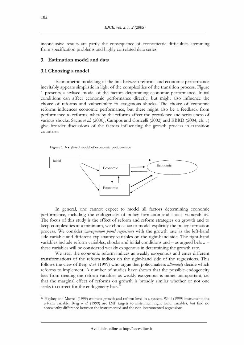

Karsten Staehr Reforms and Economic Growth in Transition Economies
Available online at httpeacesliucit
183
Initial conditions in transition countries varied tremendously Uzbekistan emerged from the Soviet Union as a mainly agricultural country with disrupted trade links Hungary in contrast has industrialised and even implemented some market-oriented reforms We generally expect initial conditions to be country specific so that the effect of initial conditions can be soaked up with fixed-effect dummies However we also perform regressions with variables reflecting initial conditions
The only control employed for exogenous shocks is a war dummy It is mainly introduced to ensure that the numerically huge negative growth rates experienced in a number of CIS and Balkan countries during war and civil unrest do not lead to extreme outliers that unduly affect results Havrylyshyn (2001) concludes in his survey that controls for shocks and initial conditions only affect slightly the estimated marginal effects of reforms
The choice of specific reform variables to be included on the right-hand side is difficult We focus on eight reform indices assembled and published by the European Bank for Reconstruction and Development (EBRD) Together with a variable reflecting nominal stability these variables broadly cover the four main areas of reforms liberalisation stabilisation privatisation and structural reforms Further the EBRD indices are available for the period 1989-2001 which permits a long estimation sample
A host of other variables have been included in growth regressions for transition countries eg measures capturing the institutional environment governance and government ability legal protection and social capital It is relatively easy to find theoretical intuitive arguments for including almost any variable Having only a limited number of data points one is forced to make difficult ndash and somewhat arbitrary ndash decisions on which variables to include and exclude
We focus on reform policies of a rather specific character The EBRD indices are ldquoestablishedrdquo in the literature allow a long sample and are all collected by the same source By omitting broader-based measures of transitional readiness we avoid complex issues related to the quality and interpretation of such variables The many variables are closely related and might to some extent be captured in the EBRD indices For example Ahrens and Meurers (2002) show that measures of governance quality are likely to affect economic outcome only via their impact on economic policies Havrylyshyn and van Rooden (2000) show that nearly all of a large number of institutional indicators are strongly correlated with the EBRD indices 32 The data set
The data set is a balanced panel consisting of annual data for 25 transition
economies from 1989 to 2001 Bosnia-Herzegovina and Yugoslavia are excluded because of data problems As in most other studies the Asian transition countries (Mongolia Vietnam and China) are not included in the data set13
The left-hand side variable G is the growth rate of the gross domestic product expressed as per cent per year The EBRD data source (various issues) relies on official statistics so data quality problems imply that output growth at the beginning of the transition is probably underestimated as new private sector activities are only partly covered (Aslund 2002 ch 4) Data that is more reliable is not available on an annual 13 Thus the panel contains data for Albania Armenia Azerbaijan Belarus Bulgaria Croatia Czech
Republic Estonia Georgia Hungary Kazakhstan Kyrgyz Republic Latvia Lithuania Macedonia Moldova Poland Romania Russia Slovakia Slovenia Tajikistan Turkmenistan Ukraine Uzbekistan
184
EJCE vol 2 n 2 (2005)
Available online at httpeacesliucit
basis but we undertake a number of robustness checks (see subsection 52) which suggest that the very large output falls in the beginning of the transition period do not affect results unduly
The right-hand side variables include consumer price inflation I measured as the annual percentage change of average consumer prices EBRD (various issues) figures are used The inflation rate can be interpreted as a measure of monetary stability and a function of stabilisation policies Data for inflation are missing for 1989-90 for countries that were still part of the Soviet Union or Yugoslavia To achieve a balanced panel these missing values are replaced with the inflation figures for the Soviet Union or Yugoslavia as appropriate This replacement has no material effect on the results To avoid extreme inflation rate observations affecting the results unduly the logarithmic transformation LI = log(100+I) is used
Several transition economies have suffered civil unrest or international conflicts The dummy WAR is equal to 1 for each year the country is engulfed in a serious domestic or international conflict If the country is at peace a value of 0 is used14
We control for initial conditions in certain cases Experimentation with individual country characteristics such as 1989 income level or the number of years under communism was unsuccessful as the variables were generally insignificant We have instead chosen to control for initial conditions with two composite variables constructed by de Melo et al (2001) INI1 captures the degree of macroeconomic distortions and unfamiliarity with market processes in society INI2 measures overall economic development in terms of industrialisation (and possible over-industrialisation) pre-reform GDP and degree of urbanisation Note that INI1 and INI2 are undated variables
The right-hand variables of most importance to this study are indices measuring reform intensity We have chosen to focus on the following indices constructed by the European Bank of Reconstruction and Development
BRIRL ndash Banking reform and interest rate liberalisation CP ndash Competition policy GER ndash Governance and enterprise restructuring LSP ndash Large-scale privatisation PL ndash Price liberalisation SMNB ndash Securities markets and non-bank financial institutions SSP ndash Small-scale privatisation TFES ndash Trade and foreign exchange system The EBRD indices capture three types of reforms PL and TFES relate to
liberalisation of the socialist economy This occurred rapidly in many countries SSP and LSP are privatisation indices measuring the transfer of production facilities to private owners The indices ignore the specific privatisation methods used The remaining four indices relate to restructuring and institution building BRIRL and SMNB measure the emergence of financial markets and the efficiency of financial intermediation GER refers to the governance structure of the firms and the degree of restructuring in principle of private as well as state-owned firms Finally CP measures the legislation and
14 The dummy is constructed using information from wwwfasorgmandod-101opswar
wwwonwarcomacedindexhtm and wwwalertnetorgthefactscountryprofiles
Karsten Staehr Reforms and Economic Growth in Transition Economies
Available online at httpeacesliucit
185
enforcement aimed at limiting misuse of monopolist power See EBRD (2001 ch 2) for a further discussion of the indices
The indices are compiled from expert assessments of EBRD staff An index score equal to 1 indicates no reform relative of a ldquostandardrdquo planned economy while the maximum score 433 corresponds to a well-functioning market economy The indices have been backdated to 1989 and data for the eight EBRD indices are thus available for the entire sample period 1989-2001 (EBRD 2000 p 31)15
Finally a trend variable is employed in all regressions to ldquopick uprdquo trended movements in G The variable TREND is equal to 1 in 1989 and increases linearly to 13 in 2001
4 Correlated reforms and principal components
We employ a large set of variables to account for economic growth in 25 transition economies the eight EBRD indices logarithmic inflation the conflict dummy and two variables capturing initial conditions Table 1 shows the correlation matrix for the ten dated variables (ie excluding initial conditions) stacked for all 25 countries
Table 1 Matrix of correlation coefficients for stacked variables
WAR LI BRIRL CP GER LSP PL SMNB SSP TFES
LI 1 033 ndash050 ndash032 ndash051 ndash045 ndash013 ndash037 ndash038 ndash044WAR 033 1 ndash027 ndash030 ndash030 ndash031 ndash018 ndash027 ndash026 ndash028BRIRL ndash027 ndash050 1 071 092 084 067 078 083 086CP ndash030 ndash032 071 1 078 074 057 078 068 063GER ndash030 ndash051 092 078 1 086 065 080 082 082LSP ndash031 ndash045 084 074 086 1 067 075 084 080PL ndash018 ndash013 067 057 065 067 1 053 079 080SMNB ndash027 ndash037 078 078 080 075 053 1 070 066SSP ndash026 ndash038 083 068 082 084 079 070 1 087TFES ndash028 ndash044 086 063 082 080 080 066 087 1Stacked variables for 25 countries 1989-2001
A distinct correlation pattern is apparent The conflict dummy is positively
correlated with logarithmic inflation and negatively with all eight EBRD indices Inflation is negatively correlated with all eight EBRD indices indicating that monetary stabilisation is positively correlated with the other reform indices Most strikingly all eight EBRD indices are positively and very strongly correlated with each other The correlation coefficients lie with few exceptions within the interval 07-08
The extent of correlation between the EBRD indices is problematic Multicollinearity can lead to erroneous inference (see Havrylyshyn 2001)16 It leads to imprecisely estimated parameters in growth regressions and makes it difficult to separate out the effects of different reforms as tests for exclusion of variables have low power17 15 The EBRD kindly supplied country-specific variables for the period 1989-90 although they have yet to
be published 16 The multicollinearity problem was already acknowledged in Fischer et al (1996b) Havrylyshyn and van
Rooden (2000) provide examples of the consequences of multicollinearity in growth regressions 17 A number of studies include an extra variable together with an overall reform variable The new
variable turns out to be highly significant while the overall reform variable becomes insignificant While
186
EJCE vol 2 n 2 (2005)
Available online at httpeacesliucit
We address the multicollinearity problem by using the principal components methodology which generates new variables (principal components) as linear combinations of the original variables The weights of the linear combinations (factor loadings) are chosen so that the new principal components are uncorrelated and so that the first principal component explains as much of the original variation as possible the second principal component explains as much as possible of the remaining variation etc18
We have chosen to calculate the principal components only for the eight EBRD indices This choice is based on three considerations First LI and WAR are not very correlated with the EBRD indices Second the resulting principal components are easier to interpret when LI and WAR are excluded Third the variables LI and WAR are primarily included as control variables because the importance of both variables is firmly established in the literature
The principal components are computed from the stacked reform indices ie the values of each of the eight EBRD indices are stacked This implies that the observations for all years weight evenly when the variance-covariance matrix (and hence the principal components) are calculated
Table 2 Principal components of eight policy reform variables
PC1 PC2 PC3 PC4 PC5 PC6 PC7 PC8
Eigenvalue 6362 0640 0320 0207 0175 0125 0109 0065Variance proportion 0795 0079 0040 0026 0022 0016 0014 0008Loadings
BRIRL 037 ndash005 ndash042 008 038 009 ndash019 070CP 033 ndash044 063 ndash038 028 ndash021 013 013GER 037 ndash016 ndash028 ndash013 035 015 ndash037 ndash068LSP 037 ndash005 ndash016 ndash049 ndash059 046 018 007PL 032 059 053 023 008 041 ndash019 001SMNB 034 ndash049 007 073 ndash032 005 009 ndash006SSP 037 026 ndash003 ndash007 ndash040 ndash069 ndash040 002TFES 036 034 ndash020 008 021 ndash024 076 ndash017Stacked variables for 25 countries 1989-2001
The result of the principal components analysis on the stacked EBRD indices is reported in Table 2 The principal components are labelled PC1 PC2hellip PC8 The upper panel shows the eigenvalues from the orthogonalisation of the sample correlation matrix and how much each principal component explains of the total variance of the primary EBRD indices (found as the eigenvalue of each principal component divided by the sum of eigenvalues) The lower panel shows the factor loadings used as weights to calculate the principal components as linear combinations of the original indices
The principal components reveal clusters of reform policies It explicates the joint structure of the reform indices and thus presents a condensed picture of the
one might conclude that the original reform variable has no impact on growth this conclusion may well be erroneous in the presence of multicollinearity
18 In technical terms the factor loadings used to calculate the uncorrelated principal components are found from an orthogonalising transformation of the sample correlation matrix The eigenvalues from the orthogonalisation reflect the share of total variation explained by each principal component
Karsten Staehr Reforms and Economic Growth in Transition Economies
Available online at httpeacesliucit
187
different reform strategies undertaken Some of the principal components have straightforward interpretations while others have less intuitive renditions The growth estimations in the next section reveal that only the following five principal components enter significantly
bull PC1 is broadly the sum of the eight reform indices divided by 3 The
variable can be interpreted as broad-based reforms including liberalisation privatisation and structural measures PC1 captures 795 of total variation in the initial eight reform variables and hence it is not without merit that many studies use an overall reform variable simply calculated as the sum of the EBRD reform indices We refer to PC1 as ldquobroad-based reformsrdquo
bull PC2 has positive factor loadings for price liberalisation market opening and small-scale privatisation It has negative loadings for the rest of the EBRD indices including the numerically large loadings for security markets and competition policy PC2 captures what is sometimes called ldquoearly reformsrdquo or ldquoinitial phase reformsrdquo (EBRD (2002)) ie liberalisation and small-scale privatisation without accompanying structural reforms PC2 is synonymous with ldquoliberalisationrdquo
bull PC6 has large positive loadings for large-scale privatisation and price liberalisation and a numerically large negative loading for small-scale privatisation ie a large PC6 indicates a large extent of large-scale privatisation relative to small-scale privatisation PC6 will be referred to as ldquolarge-scale privatisationrdquo but the principal component could just as well be defined as ldquolack of small-scale privatisationrdquo
bull PC7 is marginally significant in most of the growth regressions PC7 has large positive factors loading for market opening and substantial negative loadings for small-scale privatisation and enterprise restructuring as PC7 captures an early market opening without privatisation or restructuring of production PC7 is referred to as ldquoearly market openingrdquo
bull PC8 has a large positive loading for banking reforms and interest rate liberalisation but a large negative loading for enterprise restructuring PC8 captures a mismatch between banking and enterprise reforms and is referred to as ldquoearly bank liberalisationrdquo
The use of principal components reveals a particular structure of the reform
policies undertaken in transition economies The reform cluster PC1 where liberalisation privatisation and structural reforms are closely synchronised captures 795 of the variation in the EBRD reform indices This high share of variation is explained by the fact that all loadings are positive so PC1 retains the same trend as the underlying EBRD indices
The remaining 205 of variation is explained by PC2 hellip PC8 These principal components denote clusters where liberalisation privatisation and structural reforms do not go hand-in-hand They are examples of combinations of unsynchronised reforms19 This turns out to be useful when exploring the issues of reform complementarity For example PC2 allows us to isolate the effect of liberalisation and small-scale privatisation 19 We avoid use of the term ldquopartial reformsrdquo as it might be confused with the case where the level (or
intensity) of individual reforms is limited
188
EJCE vol 2 n 2 (2005)
Available online at httpeacesliucit
when no other reforms are pursued Similarly PC3 hellip PC8 represent different other clusters of unsynchronised reforms and allow us to consider the effect of these reform patterns
The reform clusters will ndash in different forms ndash be used as right-hand side variables in the growth regressions in following sections This use of principal components to identify clusters of reforms is relatively novel and involves a number of advantages20 It addresses effectively the multicollinearity problem which otherwise obscure inference testing of the importance of individual reform measures and of possible links between the measures
The ldquotraditionalrdquo method of detecting complementarities is to include products of different reform variables together with the reform variables themselves on the right-hand side of the regression (eg Zinne et al 2001) A significant and correctly signed parameter estimate to the multiplicative term is then interpreted as signifying a complementarity between the two reforms This method has several drawbacks First it is essentially a joint test of both a possible complementarity and the specific multiplicative relationship between the two reform variables Second the test has very low power if one or both of the variables displays very little variation Third the multiplicative term could pick up possible non-linearities which are not stemming from reform complementarities Fourth the method has also low power if there are many correlated reform variables If the multiplicative term of two reform variables is significant then the multiplicative term of two other variables strongly correlated with the first two variables will likely also be correlated Fifth the method is generally best suited for cases where there are only few reform variables which have to be interacted
This discussion suggests that the method of using multiplicative terms is less useful in our case with many correlated reform variables We propose instead using the reform clusters identified above as right-hand side variables The eight clusters represent distinct combinations of reforms which are interpretable as policy strategies cf above The weights of the individual reforms in the clusters are determined so that the resulting clusters are uncorrelated implying the clusters represent mutual exclusive reform packages21 The uncorrelated reforms clusters also imply that (linear combinations of) all the EBRD indices can be entered as right-hand side variables in the regression model We do not waste information by having to eliminate variables ex ante because of multicollinearity problems We can instead use a standard general-to-specific method of elimination of insignificant variables when specifying our empirical model
5 Reforms and economic growth performance
We can now regress the annual growth rate G on a set of right-hand variables It is customary to include contemporaneous and one-year lagged variables on the right-hand side To facilitate interpretation we implement this lag structure by including the
20 Ahrens and Meurers (2002) also apply factor analysis to stacked right-hand variables but their purpose
method and data set differ from ours Sachs et al (2000) apply a clustering method and de Melo et al (2001) principal components but in both cases only on data for initial conditions Havrylyshyn and van Rooden (2000) use the principal components method on reform data for a single year
21 Testing for complementarities implies ipso facto a cardinal comparison of variables in this case reform indices Using the standard method of multiplicative terms implies an essentially arbitrary combination of the selected indices while the principal components methodology proposed in this paper weights all reform indices so that the resulting clusters are uncorrelated ie no information need to be wasted in this case
Karsten Staehr Reforms and Economic Growth in Transition Economies
Available online at httpeacesliucit
189
contemporaneous first difference and the variable lagged one-year The first difference of a variable is indicated by a pre-imposed ∆ Employing a general-to-specific methodology we initially enter the following variables on the right-hand side G(ndash1) TREND WAR ∆LI LI(ndash1) ∆PC1 PC1(ndash1) hellip ∆PC8 PC8(ndash1)
The lagged growth rate G(ndash1) the trend variable TREND and the conflict dummy WAR are essentially control variables while the policy interest focuses on the terms involving logarithmic inflation LI and the principal components PC1 hellip PC8 In most cases we allow for country-specific fixed effects and exclude the variables capturing initial conditions INI1 and INI2 from the regression
The highly different growth paths among the countries in the sample may lead to cross-section heteroskedasticity Consequently we perform weighted least squares (WLS) estimation with cross-section weights derived from residual variances from a first-stage OLS estimation
It is important to appreciate the ldquoreduced formrdquo nature of growth regressions for transition economies In the absence of a firm theoretical foundation the exercise merely exposes correlation patterns Regarding their panel data regressions Fischer et al (1996b p 231) write ldquohellip results should be viewed as a way of describing data rather than reflecting deep structural relationsrdquo This makes it important to test the robustness of the results Thus we will later inter alia remove variables change the dynamic structure and split the sample
51 Estimation results
Even with our rich general specification a large number of variables are
significant at the 10 level (ie have numerical t-values around or above 165) the war dummy the inflation variables and one or both terms of principal components 1 2 6 7 and 8 The general-to-specific model selection is implemented by successively eliminating the variable with the numerically lowest t-value to the point where all estimates are significant at the 5 level The resulting regression is shown in column (31) in Table 3
The lagged growth rate and the trend variable are both strongly significant with positive parameters These variables most likely reflect the contribution of omitted variables in the regression However the significant lagged growth rate may also be interpreted as the result of slow adjustment to changes in the right-hand side variables Radulescu and Barlow (2002) discuss possible interpretations of this trend Unsurprisingly the parameter to the conflict dummy is negative and significant The parameters to (log) inflation changes and lagged (log) inflation are precisely estimated and have negative signs
Five principal components and in three cases their first differences survive the simplification procedure The parameter to ∆PC1 is negative while the parameter to PC1(ndash1) is positive Broad-based reforms have a short-term cost in form of lower growth the first year but are beneficial for growth from the second year onwards The parameter to ∆PC2 is negative while it is positive to PC2(ndash1) Liberalisation without accompanying reforms has a negative impact on growth in the very short term but a positive impact in the ldquomedium termrdquo ie from the second year onwards The parameters to ∆PC6 and PC6(ndash1) are both negative suggesting that accelerated large-scale privatisation is bad for growth irrespective time horizon The parameter to the term PC7(ndash1) is negative although only marginally significant Market opening without
190
EJCE vol 2 n 2 (2005)
Available online at httpeacesliucit
supporting reforms appears detrimental to growth Finally the parameter to PC8(ndash1) is also negative indicating that a policy of early bank liberalisation without enterprise reform likely affects growth negatively
Table 3 Panel data estimations of growth determinants
(31) (32) (33) (34) (35) (36)a (37)a (38) (39)
023 019 030 029 029 020 017 023G(ndash1)
(436) (277) (599) (571) (273) (222) (264) (381)033 057 020 054 039 022 049 083 040TREND
(352) (371) (201) (557) (400) (109) (211) (254) (292)ndash636 ndash624 ndash602 ndash806 ndash638 ndash796 ndash482 ndash584 ndash920WAR
(ndash374) (ndash296) (ndash330) (ndash534) (ndash330) (ndash253) (ndash179) (ndash280) (ndash606)ndash229 ndash271 ndash262 ndash237 ndash146 ndash288 ndash281 ndash276∆LI
(ndash497) (ndash361) (ndash552) (ndash432) (ndash188) (ndash471) (ndash608) (ndash475)ndash300 ndash262 ndash197 ndash418 ndash244 ndash126 ndash284 ndash363 ndash426LI(ndash1)
(ndash640) (ndash333) (ndash504) (ndash1049) (ndash489) (ndash105) (ndash269) (ndash610) (ndash691)ndash134 ndash242 ndash168 ndash132 ndash199 ndash213 ndash204 174∆PC1
(ndash302) (ndash281) (ndash351) (ndash360) (ndash202) (ndash205) (ndash459) (174)073 027 135 053 044 073 041 056 004PC1(ndash1)
(415) (083) (762) (271) (274) (190) (083) (180) (007)ndash143 ndash138 ndash191 ndash256 ndash093 ndash132 ndash137 026∆PC2
(ndash246) (ndash118) (ndash304) (ndash521) (ndash062) (ndash113) (ndash208) (035)256 378 328 238 114 485 362 263 109PC2(ndash1)
(472) (470) (751) (417) (379) (328) (334) (350) (125)ndash240 ndash135 ndash210 ndash147 ndash167 ndash149 ndash324 221∆PC6
(ndash300) (ndash089) (ndash253) (ndash182) (ndash108) (ndash108) (ndash393) (202)ndash297 ndash349 ndash047 ndash399 ndash124 ndash391 ndash288 ndash448 218PC6(ndash1)
(ndash291) (ndash203) (ndash059) (ndash399) (ndash151) (ndash149) (ndash162) (ndash306) (140)ndash142 ndash258 ndash217 ndash167 ndash188 ndash434 ndash323 050 ndash441PC7(ndash1)
(ndash205) (ndash198) (ndash304) (ndash236) (ndash272) (ndash217) (ndash164) (065) (ndash502)ndash170 ndash285 ndash133 ndash176 ndash280 ndash322 ndash233 ndash288 ndash343PC8(ndash1)
(ndash257) (ndash193) (ndash196) (ndash244) (ndash360) (ndash127) (ndash123) (ndash326) (ndash480) 1038 Constant
(389) 025 INI1
(085) ndash085 INI2
(ndash247) Method WLS OLS WLS WLS WLS GMM GMM WLS WLSSample 90-01 90-01 90-01 90-01 90-01 91-01 91-01 90-95 96-01No obs 300 300 300 300 300 300 300 150 150R2 069 070 065 067 064 059 052The growth rate G is left-hand variable All estimations except (35) are fixed-effect regressions employing country dummies t-statistics based on White Heteroskedasticity consistent standard errors are given in brackets and italics below parameter estimates a The estimated parameters are found from the differenced model using the Arellano-Bond procedure
The first results are standard for the literature (see also the discussion in section 2) Outbreaks of war and high inflation are bad for growth while overall broad-based
Karsten Staehr Reforms and Economic Growth in Transition Economies
Available online at httpeacesliucit
191
reforms are good for growth The new insights are mainly related to the estimates of the effects of unsynchronised reforms ie the effects of PC2 PC6 PC7 and PC8
52 Robustness
Column (32) in Table 3 presents the estimates obtained using ordinary pooled
least squares (OLS) instead of WLS All signs are retained but the parameter estimate to PC1(ndash1) has fallen and is now insignificant22 The estimated parameters and standard errors to ∆PC6 PC6(ndash1) PC7(ndash1) and PC8(ndash1) have also changed to some extent It seems appropriate whenever possible to use WLS
As discussed above endogeneity problems related to contemporary variables might bias the results We have re-estimated regression (31) without ∆LI ∆PC1 ∆PC2 and ∆PC6 The results reported in (33) show that the parameters to the lagged level of the variables LI(ndash1) PC1(ndash1) PC2(ndash1) PC6(ndash1) PC7(ndash1) and PC8(ndash1) have broadly retained their size and significance In practice the endogeneity problem associated with the variables based on EBRD indices is probably not serious as the indices are scored in the middle of the year when little information about the countryrsquos performance is known
Outliers could influence results unduly particularly the large negative growth rates registered for a number of CIS countries For example output contracted 526 in Armenia in 1992 This partly reflects the war in the country at that time but may also be the result of underreporting We replace the growth rate by the transformation 100G(100ndashG) which dampens the impact of large negative growth rates but has little impact on positive growth rates of ldquonormalrdquo size The findings (not shown) are close to those in column (31) so data points with extreme growth rates do not ldquodriverdquo the results Moreover experiments with transformations of other variables and inclusion of dummies to pick up outliers also show that the results are reasonably robust partly because the equations are estimated using WLS
It is relatively uncommon to include the lagged growth rate on the right-hand side of growth regressions for transition economies23 To ensure that our results do not hinge on this specification G(ndash1) is excluded and the results shown in column (34) The main effect is that the parameter to TREND increases With the exception of the parameter to PC1(ndash1) all other parameters increase somewhat numerically This result is intuitive and the medium-term impacts are broadly the same as before as the dynamic effect from the lagged growth rate is now lacking Removing the trend also has a negligible impact on the results (not shown)
To check the robustness of our results we estimate the growth equation dropping the fixed effect dummies and including instead the two variables capturing initial conditions together with a constant The results in column (35) are close to those in column (31) suggesting that the estimated impact of the reform variables is not a mirage caused by different initial conditions affecting both reform choices and growth results INI2 is significant and has the expected negative sign while INI1 is insignificant
22 The problem of obtaining a precise estimate to PC(ndash1) will reappear in a number of the specifications
used for robustness checks 23 Berg et al (1999) include the lagged growth rate on the right-hand side of the regression but find that it
is insignificant
192
EJCE vol 2 n 2 (2005)
Available online at httpeacesliucit
OLS-based estimation methods can yield biased estimates in dynamic panels due to correlation between the country-specific fixed effects and the error term There is still no consensus on which estimation method to use in this case The often-used Arellano-Bond GMM method first eliminates country-specific effects by differencing the equation and then use lagged values of the level variables as GMM instruments24
However GMM estimation like the Arellano-Bond method gives rise to bias in small samples in particular when right-hand side variables are serially correlated Indeed Judson and Owen (1999) show that in a sample with few cross-sections and a short time horizon the Arellano-Bond method performs no better than the fixed-effect OLS estimator (although better than standard OLS without fixed effects) Other methods are likely to perform better depending on the structure of data Beck and Levine (2004) point out that estimates from the Arellano-Bond method could be strongly biased in small-sample dynamic panels with persistent right-hand side variables Nerlove (2002) argues that the Arellano-Bond method is inappropriate in dynamic panels with a short time dimension and examines the properties of a number of other methods without finding any generally superior estimator 25
As a robustness check we estimate the dynamic model with trend using the Arellano-Bond GMM method In the first case we only instrument the lagged growth rate assuming that the contemporaneous right-hand variables (∆LI ∆PC1 ∆PC2 and ∆PC6) are weakly exogenous The results using the Arellano-Bond one-step method are presented in column (36) Although some changes occur the results in (36) are broadly in line with the results of the WLS estimation in (31) and with the OLS estimation in (33) (Note that the Arellano-Bond procedure implies that the sample is reduced one period)
Column (37) shows the results when the contemporaneous variables (∆LI ∆PC1 ∆PC2 and ∆PC6) are also instrumented using Arelleno-Bond level instruments This should eliminate possible endogeneity biases from the contemporaneous right-hand variables Again the changes are not dramatic
The conclusion is that GMM estimation confirms the qualitative results obtained earlier The estimated standard errors are generally larger for the GMM estimations than for the OLSWLS estimations This problem is to some extent related to the ldquoweak instrument problemrdquo causing the GMM estimators to be inefficient in small samples26 We find as do several other studies that the GMM results are not fundamentally different from least-squares-based methods They may however suffer from inference problems
When the sample is split into two subperiods some instability is revealed The estimation results are shown for 1990-95 in column (310) and for 1996-2001 in column (311) The estimation results for the early subperiod correspond closely to the full sample results with the exception of the estimate to PC7(ndash1) which is positive albeit insignificant For the latter subperiod a number of changes are noteworthy First the 24 Instrumentation is required as the error term of the difference equation is still correlated with the left-
hand side variable 25 This is also reflected in eg Pattillo et al (2002) where dynamic growth models are estimated All results
are presented using four different estimation techniques including GMM 26 The use of the Arellano-Bond method is not rejected There is first-order autocorrelation in the
residuals in the differenced model and the Sargan test does not reject the instruments Nevertheless the presence of serially correlated right-hand variables reduces the efficiency of the level instruments The potential small-sample bias is an argument for avoiding a general-to-specific specification search using GMM
Karsten Staehr Reforms and Economic Growth in Transition Economies
Available online at httpeacesliucit
193
parameters to ∆PC1 and ∆PC2 are now positive although none of the variables are significant at the 5 level The short-term costs of reforms seem at most to be a feature of the early stages of transition Second the estimated parameters to PC1(ndash1) and PC2(ndash1) have dropped substantially However the changes to the parameters to ∆PC1 and ∆PC2 combined with the changes to PC1(ndash1) and PC2(ndash1) imply that the effects of the two reform clusters in the 2-4 years interval are broadly unchanged What has changed is merely the adjustment dynamics Third ∆PC6 and PC6(ndash1) have changed sign while PC7(ndash1) is highly significant in the late period In sum reforms do a better job of explaining growth at the beginning of the reform period than at the end A number of studies reach this conclusion eg Radulescu and Barlow (2002) This is consistent with the view that reforms change the structure of these economies likely increasing the importance of traditional growth factors like physical and human capital accumulation
The estimations reported employ ldquocalendar timerdquo Calendar time ndash as opposed to ldquotransition timerdquo ndash is chosen because it gives the longest possible sample ensures more variation in both right-hand and left-hand variables and simplifies interpretation in certain cases As a robustness check most of the regressions in this paper have been re-estimated using transition time using the correspondence suggested in Berg et al (1999) The results (not shown) are broadly similar to those reported The main difference is that the estimates to ∆PC1 and ∆PC2 although still negative tend not to be significant at conventional levels This result is broadly in line with the above finding that the negative and significant parameters to ∆PC1 and ∆PC2 are derived from the early part of the sample (which is shortened for many countries when transition time is used)27
53 Results and discussion
The broadly similar results obtained from many specifications suggest that
several fairly robust conclusions can be drawn concerning the relationship between reforms and growth in transition countries The control variables offer straightforward interpretations Conflict situations affect growth negatively while the lagged growth rate and a trend always attain positive signs
Inflation and increasing inflation are negatively correlated with growth The contemporaneous effect of inflation changes is negative even in the later half of the sample ie there still appears to be no short-term Phillips curve relationship in the transition economies
We find that broad-based reforms as represented by principal component PC1 are good for growth in the medium term while the short-term effect may be negative at the early stages of reform The parameter to PC1(ndash1) has been estimated to values ranging from 022 to 073 (and 135 in an extremely under-parameterised model) This rather broad interval of estimates is somewhat inconvenient as PC1 captures the overall reform progress and different parameter sizes have different implications for the desirability of reforms28
27 Additional robustness tests can be found in the working paper version of this paper Staehr (2003) 28 The result is however consistent with previous contributions which have found a wide range of
estimated parameter values to a broad index of reforms (see discussion in Radulescu and Barlow 2002) Radulescu and Barlow (2002) use an extreme bounds analysis and show that the sum of the EBRD indices does not enter robustly in their growth regressions ie the parameter and the significance of the
194
EJCE vol 2 n 2 (2005)
Available online at httpeacesliucit
Early reforms in the form of liberalisation and small-scale privatisation have a positive medium-term effect on growth even in the absence of other (mainly structural) reforms Liberalisation and small-scale privatisation have a positive effect on growth even if structural reforms are less advanced The short-term impact of early liberalisation appears to be negative at the early stages of reform
A policy of large-scale privatisation and price liberalisation without small-scale privatisation and market opening has a negative impact on growth The impact is contemporaneous as well as medium-term This result broadly confirms the finding in Zinnes et al (2001) that privatisation without enterprise reforms leads to title change with little restructuring Broadly similar results follow from the meta-analysis in Djankov and Murrell (2002) of approximately 100 empirical studies examining restructuring at the enterprise level Fast privatisation of large firms with insufficient supporting reforms hold back firm restructuring and growth (see also Havrylyshyn 2001) Note however that the result implies rapid small-scale privatisation is beneficial to growth even in the absence of large-scale privatisation and price liberalisation
Early market opening without other reforms like small-scale privatisation and enterprise restructuring also seems detrimental to growth at least in the latter part of transition Figuratively one might imagine foreign competition sweeping away domestic state-owned and unreconstructed producers Crafts (2000) and IMF (1997) discuss preconditions necessary to ensure that market opening and international integration is beneficial to growth Again the reasoning can be reversed a policy of small-scale privatisation and enterprise restructuring appear growth enhancing minus even when not backed by market opening
Finally bank liberalisation without enterprise restructuring has a negative impact on growth especially in the later stages of reform An example of this might be the Czech experience in the mid-1990s when excessive bank lending to non-restructured firms contributed to serious banking sector problems and unsatisfactory growth (see OECD 1998 and 2000) The reverse interpretation is that enterprise restructuring is beneficial even in the absence of bank liberalisation
6 Speed of reforms
The speed at which reforms should be introduced and implemented remains a controversial issue within transition economics The debate also covers sequencing and reform complementary as sequenced reforms may take longer to implement than broad-based reforms This section focuses on the effect on growth of speed per se ie the overall speed with which reforms are implemented29
As noted in section 2 an argument for speedy reform exists when the reform level affects growth positively Fast reforms would put the country on a higher path early on allowing the country to enjoy higher growth for a longer period In this sense all estimations presented in section 5 suggest that broad-based reforms (PC1) or
parameter depend on other variables in the regressions Fidrmuc (2003) also found that it is difficult to estimate the parameter to broad-based reforms precisely
29 The speed of reforms is also important for objectives other than growth eg distribution regional development and medium-term political sustainability These issues cannot be addressed in this framework
Karsten Staehr Reforms and Economic Growth in Transition Economies
Available online at httpeacesliucit
195
liberalisation (PC2) should be implemented rapidly30 However as argued in section 2 we are interested in effects on top of this level effect
Testing directly for speed effects presents two challenges We must specify precise and testable hypotheses and then derive and implement tests of those hypotheses Here we consider two hypotheses First speed effects may affect the level of ldquopainrdquo resulting from reforms in the short term Second the speed of reforms may affect medium-term growth and therefore influence the selection of growth path The short-term hypothesis is examined by testing for possible convexity in the short-term reform costs The medium-term hypothesis is tested by the construction of variables that capture respectively the divergence of the actual reform level from the trend level and indicator variables for a countryrsquos rate of reform
61 Non-linearities in short-term costs
The estimations in section 5 implicitly assumed that short-term reform changes
affect growth rates linearly This assumption implies that the short-term costs of reforms are the same whether reforms are implemented quickly or done piecemeal over several years However possible convexities in the short-term impact would imply ceteris paribus that the level of transition ldquopainrdquo might be lower in a slow reform regime
The search for short-term convexities is narrowed to the first two principal components The starting point for our search for convexities is regression (31) in Table 3 For ease of comparison we repeat this regression in column (41) in Table 4 We test first for possible convexities in the link between ∆PC1 and growth ∆PC1 is replaced by the transformation (137+∆PC1)α where α is the parameter allowing for non-linear effects and 137 is added to ensure that the argument is always positive We perform a grid search by varying α = 01 02 hellip searching for the α-value leading to the parameter estimate with the highest t-value The result is shown in column (42) in Table 4 A similar procedure is performed for ∆PC2 with β varied to give the most precise estimate of (141+∆PC2)β The result appears in column (43)
For the term containing ∆PC1 the t-value was maximised for α = 123 while the t-value for the term containing ∆PC2 was maximised for β = 16 There seems to be a high degree of convexity in the short-term growth costs of broad-based reform and a moderate degree in the liberalisation term
The results are obtained in spite of the test being biased against detecting non-linear effects as only linear variables were used in the specification search Still the test has little power In the specification shown in (42) we have added ∆PC1 as a separate right-hand side variable to ldquocompeterdquo with (137+∆PC1)123
The parameters to both (137+∆PC1)123 and ∆PC1 are negative but insignificant A Wald test cannot reject the joint hypothesis that the parameter to (137+∆PC1)123 is 0 and the parameter to ∆PC1 is ndash229 (as in the original specification) We conclude that although the convex specification yields a slightly more precise parameter estimate the difference is not statistically significant The same holds for the convex specification of ∆PC2
30 Naturally the opposite holds for the unsynchronised reforms of the types captured by PC6 PC7 and
PC8
196
EJCE vol 2 n 2 (2005)
Available online at httpeacesliucit
Table 4 Speed effects in panel data estimations of growth determinants
(41)a (42) (43) (44) (45) (46)
023 026 023 032 027 027G(ndash1)
(436) (498) (436) (553) (549) (568)033 030 033 042 060 070TREND
(352) (342) (352) (271) (541) (643)ndash636 ndash594 ndash642 ndash314 ndash647 ndash633WAR
(ndash374) (ndash387) (ndash381) (ndash155) (ndash330) (ndash319)ndash229 ndash232 ndash222 ndash132 ndash243 ndash243∆LI
(ndash497) (ndash559) (ndash486) (ndash228) (ndash441) (ndash445)ndash300 ndash310 ndash298 ndash219 ndash262 ndash265LI(ndash1)
(ndash640) (ndash741) (ndash642) (ndash324) (ndash518) (ndash536)ndash134 ndash117 ndash001 ndash151 ndash162∆PC1
(ndash302) (ndash254) (ndash002) (ndash420) (ndash502)073 082 073 023 036 039PC1(ndash1)
(415) (496) (412) (053) (232) (276)ndash143 ndash123 142 ndash249 ndash247∆PC2
(ndash246) (ndash206) (193) (ndash511) (ndash551)256 238 246 351 108 080PC2(ndash1)
(472) (488) (450) (454) (350) (260)ndash240 ndash291 ndash241 ndash227 ndash137 ndash142∆PC6
(ndash300) (ndash369) (ndash302 (ndash207) (ndash171) (ndash185)ndash297 ndash312 ndash301 ndash169 ndash128 ndash115PC6(ndash1)
(ndash291) (ndash319) (ndash295) (ndash115) (ndash161) (ndash150)ndash142 ndash121 ndash147 ndash280 ndash187 ndash170PC7(ndash1)
(ndash205) (ndash177) (ndash209) (ndash269) (ndash280) (ndash251)ndash170 ndash116 ndash165 ndash105 ndash217 ndash208PC8(ndash1)
(ndash257) (ndash173) (ndash248) (ndash124) (ndash273) (ndash276) ndash313middot10ndash8 (137 + ∆PC1)123
(ndash436) ndash08 (141 + ∆PC2)16
(ndash262) 012 PC1SP
(062) 1038 1006Constant
(392) (387) 003 INI1
(009) ndash098 INI2
(ndash290) ndash054 YEAR
(ndash414) ndash377FAST
(ndash688) ndash312SLOW
(ndash503)Method WLS WLS WLS WLS WLS WLSSample 90-01 90-01 90-01 93-01 90-01 90-01No observations 300 300 300 225 300 300R2 069 068 069 062 066 066The growth rate G is left-hand variable t-statistics based on White Heteroskedasticity consistent standard errors are given in brackets and italics below parameter estimates a For ease of comparison column (41) repeats column (31) from Table 3
Karsten Staehr Reforms and Economic Growth in Transition Economies
Available online at httpeacesliucit
197
62 Divergence from trend reform path We construct a variable that directly reflects the speed of reforms based on a
suggestion in Berg et al (1999) The idea is to calculate the trend reform level during a fixed time window and then compare the actual reform level with the calculated trend value during the early part of the window The higher the early reform level is above trend level the speedier the implementation of reforms
The implementation speed of broad-based reforms is considered within a four-year window We follow the convention in econometrics and use no time indication of the current realisation of a variable We use τ to indicate years from current year Thus τ = 0 indicates the current year τ = ndash1 indicates a one year lag τ = ndash2 indicates a two year lag etc With this notation the contemporaneous reform level is PC1 and the reform level in year τ ie the reform level lagged τ years is PC1(τ)
We consider a four-year window preceding the current year The total change in the reform index during the four year period is [PC1 ndash PC1(ndash4)] and the average annual change is [PC1 ndash PC1(ndash4)]4 Accordingly the expected trend reform level for any year in the four-year window preceding the current year is
EPC1(τ) = PC1(ndash4) + (4 + τ)middot[PC1 ndash PC1(ndash4)]4 where τ = ndash4 hellip ndash1 For τ = ndash4 EPC1(τ) = PC1(τ) while EPC1(τ) increases
linearly with the annual rate of reform change for τ = ndash3 ndash2 ndash1 The speed variable PC1SP is the sum of the differences between the actual and the trend reform level for years τ = ndash3 and τ = ndash2
PC1SP = [PC1(ndash3) ndash EPC1(ndash3)] + [PC1(ndash2) ndash EPC1(ndash2)] PC1SP is added to specification (31) with the result shown in column (44) in
Table 4 Note that the sample period has changed as PC1SP absorbs three years of the sample The parameter to PC1SP is positive but insignificant31 It should be noted however that the regression contains many variables which could make it difficult for PC1SP to attain significance The partial correlation between G and PC1SP is positive and highly significant Still experiments with different samples non-linear transformations and lagged values of PC1SP show that no stable relationship exists On the suspicion of asymmetric effects we split PC1SP into two variables respectively containing positive and negative values but the results (not shown) were again inconclusive Similar exercises using the liberalisation cluster (PC2) fail to yield any consistent results
63 Scoring of reform speed
Finally we apply methods derived from Wolf (1999) to test for speed effects Initially the number of years from the start of the reform process (ie year 0 using
31 The parameter to ∆PC1 is now insignificant This is the consequence of the shorter sample (also see
(39) in Table 3) and the exclusion of PC1SP
198
EJCE vol 2 n 2 (2005)
Available online at httpeacesliucit
transition time) until PC1 has increased by 4 is counted32 This number (score) would be eg 2 for the Czech Republic and Estonia 4 for Hungary and Moldova and 7 for Bulgaria and Croatia For some countries eg Belarus and Macedonia PC1 does not increase by 4 units within by 2001
The variable YEAR is constructed as follows For 1989-1997 it contains zeros for 1998-2001 it contains the speed score provided the score is less than 8 otherwise zero The construction of YEAR with zeros until 1998 implies that only medium-term effects of the speed score are captured and ensures that the measure of reform speed does not affect growth before reforms are actually implemented33
We include YEAR in regression (35) with a constant term and controls for initial conditions (Fixed effects estimation cannot be used when YEAR is included) The result is shown in column (45) in Table 4 The estimated parameter is negative and significant indicating that reform speed is positively correlated with growth ie rapid reform is associated with higher medium-term growth
Another test separates the transition countries into three groups The first group consists of countries undertaking fast reforms (YEAR le 3) the second group consists of countries undertaking gradual reforms (4 le YEAR le 7) and the third group contains reform-resistant laggards (YEAR ge 8) The dummy FAST has zeros for 1989-97 and ones for 1998-2001 for all countries in the first group The dummy SLOW has zeros for 1989-97 and ones for countries in the second group Column (46) in Table 4 shows the result of adding these two dummy variables to regression (35) Both have negative (and significant) parameters The parameter to FAST is smaller than to SLOW which may indicate that slow reforms were beneficial to growth However the Wald test cannot reject the hypothesis that the two parameters are identical
The method of directly inserting the variables YEAR or FAST and SLOW into the growth regression did not provide firm evidence on the effect of speed However there is no evidence that speedy reforms hampered medium-term growth
64 Discussion
Early reforms allow more years in which the transition country can reap the benefits Beyond this trivial finding the panel data methodology employed in this paper does not provide strong arguments for or against rapid reform The short-term cost of reforms might be larger when implemented in bulk but the effect is small and insignificant The medium-term growth effects of rapid reform are uncertain but rapid reforms appear unlikely to hamper growth In sum the speed of reforms does not appear to a quantitatively substantial impact on growth over and above the level effect This result is in conflict with the conclusions in World Bank (1996) and Berg et al (1999) but is broadly in line with Wolf (1999)
32 For a country starting with all reform indices at their lowest level (eg most countries emerging from
the Soviet Union) an increase of PC1 equal to 4 signifies that the country is halfway to a well-developed market economy
33 It also implies that the variable YEAR only contributes to explaining growth in the last four years of the sample 1990-2001 ie the part of the sample where the other right-hand variables are relative less effective
Karsten Staehr Reforms and Economic Growth in Transition Economies
Available online at httpeacesliucit
199
7 Final comments
A novel feature of this paper was the use of principal component clustering of the EBRD reform indices to infer the structure of reform in transition economies A cluster of synchronised broad-based reforms ie liberalisation privatisation and structural reforms covers 795 of all variation in the initial EBRD reform indices A cluster of liberalisation and small-scale reforms without other reforms explains 79 of the variation while six other clusters of unsynchronised reforms span the remaining 126
The growth regressions included the reform clusters inflation terms and control variables As in most other studies inflation was found to be detrimental to growth Synchronised broad-based reforms had a positive impact on growth in the medium term with a negative short-term effect at the early stages of reform Also a policy of liberalisation and small-scale privatisation without accompanying structural reforms were shown to have a positive effect (again with a possible early negative short-term effect) Accelerated large-scale privatisation without small-scale privatisation and structural reforms were found likely to harm growth both in the short and the medium term
Conversely small-scale privatisation without large-scale privatisation appears beneficial to growth A less certain result is that market opening and price liberalisation without accompanying privatisation and enterprise reforms appear correlated with lower growth but this effect stems primarily for the most recent period Reversing this result privatisation and restructuring without market opening may be good for growth Finally bank liberalisation without enterprise restructuring might be harmful while enterprise reforms without bank liberalisation may increase growth
Effects from the speed of reforms are mostly absent with the exception that early reforms leave the transition country a longer period in which to reap the benefits of reforms Possible negative short-term effects of rapid reforms are likely to be modest and could be balanced by possible positive medium-term effects The broad overall conclusion is that speed per se has no discernible impact on growth
Finally what can we now say about the three questions raised in the introduction
First the analysis revealed a complex pattern of reform complementarities with notable implications for the sequencing of reforms Balanced wide-ranging reforms based on simultaneous progress in liberalisation privatisation and structural reforms are favourable to growth and hence suggest a mutually reinforcing effect of various reform elements
Liberalisation combined with small-scale privatisation is beneficial even in the absence of other reforms In this case unsynchronised reforms produce positive growth effects Thus liberalisation and small-scale privatisation are not perfectly complementary to deeper reforms such as large-scale privatisation and structural reforms A sequenced reform policy that stresses liberalisation and small-scale privatisation is beneficial Early ldquoeasyrdquo reforms should therefore not be postponed in the absence of a comprehensive reform strategy
A number of unsynchronised reform packages proved detrimental to growth Sequenced policy packages involving large-scale privatisation without small-scale privatisation market opening without accompanying reforms and bank liberalisation without enterprise restructuring lead to lower growth in the short andor medium term Conversely a ldquoreversalrdquo of the policy mix would produce packages beneficial to growth
200
EJCE vol 2 n 2 (2005)
Available online at httpeacesliucit
In sum the statistically significant parameters to a number of unsynchronised reform clusters support the view that reforms need to be fine-tuned to take into account complex interactions among reforms
Second we asked which reforms are of foremost importance Within the set of variables used in this paper and using a broad brush a number of variables stand out Inflation stabilisation repeatedly proved important Price liberalisation small-scale privatisation enterprise restructuring (and to a lesser degree trade opening) were generally important in many different combinations with other reforms Large-scale privatisation financial sector reforms and market regulation mainly proved beneficial when they were part of a larger more comprehensive reform packages These results seem to support the view that reform policies are crucial minus even countries that fail to attempt deep structural changes can gain from reforms These findings are broadly in line with the findings in Havrylyshyn and van Rooden (2000) As a caveat we note that only a few variables included in our analysis reflect currently popular themes such as institutional quality and social capital
Third the finding that speed per se is of little importance for growth seems to favour relatively rapid implementation of reforms due to the level effect However this finding also implies there is no direct loss from slowing reforms when it is necessary to get content or sequencing right
These results probably disappoint supporters of big-bang as well as supporters of gradualism as they provide no unequivocal support for either view If it is any consolation to the gradualists reform sequencing appears to be important and reforms should preferably progress synchronously Certain sequenced reform paths are clearly counterproductive Likewise for the big-bang supporters initial phase reforms are beneficial even in the absence of deeper reforms Moreover fast reforms appear generally beneficial Thus there is no clear-cut transition strategy that provides the best results for countries endeavouring to convert a centrally planned economy into a market economy There are only policy choices minus some better than others minus and certain strategies that should be avoided
References
Ahrens J Meurers M (2002) lsquoHow Governance Affects the Quality of Policy Reform and Economic Performance New Evidence for Economies in Transitionrsquo Journal for Institutional Innovation Development and Transition 6 35-56
Aslund A (2002) Building Capitalism The Transformation of the Former Soviet Bloc Cambridge University Press Cambridge
Aziz J Wescott R (1997) lsquoPolicy Complementarities and the Washington Consensusrsquo IMF Working Paper No118
Beck T Levine R (2004) lsquoStock Markets Banks and Growth Panel Evidencersquo Journal of Banking and Finance 28 423-442
Berg A Borensztein E Sahay R Zettelmeyer J (1999) lsquoThe Evolution of Output in the Transition Economies Explaining the Differencesrsquo IMF Working Paper No73
Blanchard O Dornbusch R Krugman P Layard R Summers L (1991) Reform in Eastern Europe MIT Press Cambridge MA
Campos N Coricelli F (2002) lsquoGrowth in Transition What We Know What We Donrsquot and What We Shouldrsquo Journal of Economic Literature 90 793-836
Karsten Staehr Reforms and Economic Growth in Transition Economies
Available online at httpeacesliucit
201
Correa R (2002) lsquoThe Washington Consensus in Latin America A Quantitative Evaluationrsquo mimeo San Francisco de Quito University Ecuador
Crafts N (2000) lsquoGlobalization and Growth in the Twentieth Centuryrsquo in Prasad E (ed) Supporting Studies for the World Economic Outlook International Monetary Fund Washington DC
de Melo M Denizer C Gelb A (1997) lsquoFrom Plan to Market Patterns of Transitionrsquo in Blejer M Skreb M (eds) Macroeconomic Stabilization in Transition Economies Cambridge University Press Cambridge
de Melo M Denizer C Gelb A (2001) lsquoCircumstance and Choice The Role of Initial Conditions and Policies in Transition Economiesrsquo World Bank Economic Review 15 1-31
Djankov S Murrell P (2002) lsquoEnterprise Restructuring in Transition A Quantitative Surveyrsquo Journal of Economic Literature 90 739-792
EBRD (1999-2004) Transition Report European Bank for Reconstruction and Development Fidrmuc J (2003) lsquoEconomic Reform Democracy and Growth during Post Communist
Transitionrsquo European Journal of Political Economy 19 583-604 Fischer S Gelb A (1991) lsquoThe Process of Socialist Economic Transformationrsquo Journal of
Economic Perspectives 5 91-105 Fischer S Sahay R (2000) lsquoThe Transition Economies After Ten Yearsrsquo IMF Working Paper
No30 Fischer S Sahay R Vegh C (1996a) lsquoStabilization and Growth in Transition Economies The
Early Experiencersquo Journal of Economic Perspectives 10 45-66 Fischer S Sahay R Vegh C (1996b) lsquoEconomies in Transition The Beginnings of Growthrsquo
American Economic Review 86 229-233 Havrylyshyn O van Rooden R (2000) lsquoInstitutions Matter in Transition but so do Policiesrsquo
IMF Working Paper No70 Havrylyshyn O (2001) lsquoRecovery and Growth in Transition A Decade of Evidencersquo IMF Staff
Paper 48 53-87 Havrylyshyn O Izvorski I van Rooden R (1998) lsquoRecovery and Growth in Transition
Economies 1990-97 A Stylized Regression Analysisrsquo IMF Working Paper No141 Heybey B Murrell P (1999) lsquoThe Relationship Between Economic Growth and the Speed of
Liberalization During the Transitionrsquo Policy Reform 3 121-37 IMF (1997) World Economic Outlook Globalization Opportunities and Challenges May chapter IV IMF (2000) World Economic Outlook Focus on Transition Economies October chapter III Judson R Owen A (1999) lsquoEstimating Dynamic Panel Data Models A Practical Guide for
Macroeconomistsrsquo Economics Letters 65 9-15 Nerlove M (2002) lsquoProperties of Alternative Estimators of Dynamic Panel Models An
Empirical Analysis of Cross-Country Data for the Study of Economic Growthrsquo in Nerlove M Essays in Panel Data Econometrics Cambridge University Press Cambridge
Nsouli S Rached M Funke N (2002) lsquoThe Speed of Adjustment and the Sequencing of Economic Reforms Issues and Guidelines for Policymakersrsquo IMF Working Paper No132
OECD (1998) OECD Economic Surveys Czech Republic May OECD OECD (2000) OECD Economic Surveys Czech Republic February OECD Pattillo C Poirson H Ricca L (2002) lsquoExternal Debt and Growthrsquo IMF Working Paper No69 Radulescu R Barlow D (2002) lsquoThe Relation between Policies and Growth in Transition
Countriesrsquo Economics of Transition 10 719-745 Roland G (2001) lsquoTen Years After hellip Transition and Economicsrsquo IMF Staff Papers 48 29-52
202
EJCE vol 2 n 2 (2005)
Available online at httpeacesliucit
Sachs J Zinnes G Eilat Y (2000) lsquoPatterns of Economic Reform and its Determinants in Transition Economies 1990-1998rsquo Harvard Institute for International Development CAER II Discussion Paper No 61
Staehr K (2003) lsquoReforms and Economic Growth in Transition Economies Complementarity Sequencing and Speedrsquo BOFIT Discussion Paper No1
Stiglitz J (2001) lsquoWhither Reform Ten Years of Transitionrsquo in Pleskovic B Stiglitz J (eds) World Bank Annual Bank Conference on Development Economics 1999 World Bank Washington DC
Wacziarg R (2002) lsquoReview of Easterlyrsquos The Elusive Quest for Growthrsquo Journal of Economic Literature 90 907-918
Wolf H (1999) lsquoTransition Strategies Choices and Outcomesrsquo Princeton Studies in International Finance No85
World Bank (1996) World Development Report 1996 From Plan to Market World Bank Washington DC
World Bank (2002) Transition The First Ten Years Analysis and Lessons for Eastern Europe and the former Soviet Union World Bank Washington DC
Zinnes C Eilat Y Sachs J (2001) lsquoThe Gains from Privatization in Transition Economies Is lsquoChange of Ownershiprsquo Enoughrsquo IMF Staff Papers 48 146-169

Karsten Staehr Reforms and Economic Growth in Transition Economies
Available online at httpeacesliucit
185
enforcement aimed at limiting misuse of monopolist power See EBRD (2001 ch 2) for a further discussion of the indices
The indices are compiled from expert assessments of EBRD staff An index score equal to 1 indicates no reform relative of a ldquostandardrdquo planned economy while the maximum score 433 corresponds to a well-functioning market economy The indices have been backdated to 1989 and data for the eight EBRD indices are thus available for the entire sample period 1989-2001 (EBRD 2000 p 31)15
Finally a trend variable is employed in all regressions to ldquopick uprdquo trended movements in G The variable TREND is equal to 1 in 1989 and increases linearly to 13 in 2001
4 Correlated reforms and principal components
We employ a large set of variables to account for economic growth in 25 transition economies the eight EBRD indices logarithmic inflation the conflict dummy and two variables capturing initial conditions Table 1 shows the correlation matrix for the ten dated variables (ie excluding initial conditions) stacked for all 25 countries
Table 1 Matrix of correlation coefficients for stacked variables
WAR LI BRIRL CP GER LSP PL SMNB SSP TFES
LI 1 033 ndash050 ndash032 ndash051 ndash045 ndash013 ndash037 ndash038 ndash044WAR 033 1 ndash027 ndash030 ndash030 ndash031 ndash018 ndash027 ndash026 ndash028BRIRL ndash027 ndash050 1 071 092 084 067 078 083 086CP ndash030 ndash032 071 1 078 074 057 078 068 063GER ndash030 ndash051 092 078 1 086 065 080 082 082LSP ndash031 ndash045 084 074 086 1 067 075 084 080PL ndash018 ndash013 067 057 065 067 1 053 079 080SMNB ndash027 ndash037 078 078 080 075 053 1 070 066SSP ndash026 ndash038 083 068 082 084 079 070 1 087TFES ndash028 ndash044 086 063 082 080 080 066 087 1Stacked variables for 25 countries 1989-2001
A distinct correlation pattern is apparent The conflict dummy is positively
correlated with logarithmic inflation and negatively with all eight EBRD indices Inflation is negatively correlated with all eight EBRD indices indicating that monetary stabilisation is positively correlated with the other reform indices Most strikingly all eight EBRD indices are positively and very strongly correlated with each other The correlation coefficients lie with few exceptions within the interval 07-08
The extent of correlation between the EBRD indices is problematic Multicollinearity can lead to erroneous inference (see Havrylyshyn 2001)16 It leads to imprecisely estimated parameters in growth regressions and makes it difficult to separate out the effects of different reforms as tests for exclusion of variables have low power17 15 The EBRD kindly supplied country-specific variables for the period 1989-90 although they have yet to
be published 16 The multicollinearity problem was already acknowledged in Fischer et al (1996b) Havrylyshyn and van
Rooden (2000) provide examples of the consequences of multicollinearity in growth regressions 17 A number of studies include an extra variable together with an overall reform variable The new
variable turns out to be highly significant while the overall reform variable becomes insignificant While
186
EJCE vol 2 n 2 (2005)
Available online at httpeacesliucit
We address the multicollinearity problem by using the principal components methodology which generates new variables (principal components) as linear combinations of the original variables The weights of the linear combinations (factor loadings) are chosen so that the new principal components are uncorrelated and so that the first principal component explains as much of the original variation as possible the second principal component explains as much as possible of the remaining variation etc18
We have chosen to calculate the principal components only for the eight EBRD indices This choice is based on three considerations First LI and WAR are not very correlated with the EBRD indices Second the resulting principal components are easier to interpret when LI and WAR are excluded Third the variables LI and WAR are primarily included as control variables because the importance of both variables is firmly established in the literature
The principal components are computed from the stacked reform indices ie the values of each of the eight EBRD indices are stacked This implies that the observations for all years weight evenly when the variance-covariance matrix (and hence the principal components) are calculated
Table 2 Principal components of eight policy reform variables
PC1 PC2 PC3 PC4 PC5 PC6 PC7 PC8
Eigenvalue 6362 0640 0320 0207 0175 0125 0109 0065Variance proportion 0795 0079 0040 0026 0022 0016 0014 0008Loadings
BRIRL 037 ndash005 ndash042 008 038 009 ndash019 070CP 033 ndash044 063 ndash038 028 ndash021 013 013GER 037 ndash016 ndash028 ndash013 035 015 ndash037 ndash068LSP 037 ndash005 ndash016 ndash049 ndash059 046 018 007PL 032 059 053 023 008 041 ndash019 001SMNB 034 ndash049 007 073 ndash032 005 009 ndash006SSP 037 026 ndash003 ndash007 ndash040 ndash069 ndash040 002TFES 036 034 ndash020 008 021 ndash024 076 ndash017Stacked variables for 25 countries 1989-2001
The result of the principal components analysis on the stacked EBRD indices is reported in Table 2 The principal components are labelled PC1 PC2hellip PC8 The upper panel shows the eigenvalues from the orthogonalisation of the sample correlation matrix and how much each principal component explains of the total variance of the primary EBRD indices (found as the eigenvalue of each principal component divided by the sum of eigenvalues) The lower panel shows the factor loadings used as weights to calculate the principal components as linear combinations of the original indices
The principal components reveal clusters of reform policies It explicates the joint structure of the reform indices and thus presents a condensed picture of the
one might conclude that the original reform variable has no impact on growth this conclusion may well be erroneous in the presence of multicollinearity
18 In technical terms the factor loadings used to calculate the uncorrelated principal components are found from an orthogonalising transformation of the sample correlation matrix The eigenvalues from the orthogonalisation reflect the share of total variation explained by each principal component
Karsten Staehr Reforms and Economic Growth in Transition Economies
Available online at httpeacesliucit
187
different reform strategies undertaken Some of the principal components have straightforward interpretations while others have less intuitive renditions The growth estimations in the next section reveal that only the following five principal components enter significantly
bull PC1 is broadly the sum of the eight reform indices divided by 3 The
variable can be interpreted as broad-based reforms including liberalisation privatisation and structural measures PC1 captures 795 of total variation in the initial eight reform variables and hence it is not without merit that many studies use an overall reform variable simply calculated as the sum of the EBRD reform indices We refer to PC1 as ldquobroad-based reformsrdquo
bull PC2 has positive factor loadings for price liberalisation market opening and small-scale privatisation It has negative loadings for the rest of the EBRD indices including the numerically large loadings for security markets and competition policy PC2 captures what is sometimes called ldquoearly reformsrdquo or ldquoinitial phase reformsrdquo (EBRD (2002)) ie liberalisation and small-scale privatisation without accompanying structural reforms PC2 is synonymous with ldquoliberalisationrdquo
bull PC6 has large positive loadings for large-scale privatisation and price liberalisation and a numerically large negative loading for small-scale privatisation ie a large PC6 indicates a large extent of large-scale privatisation relative to small-scale privatisation PC6 will be referred to as ldquolarge-scale privatisationrdquo but the principal component could just as well be defined as ldquolack of small-scale privatisationrdquo
bull PC7 is marginally significant in most of the growth regressions PC7 has large positive factors loading for market opening and substantial negative loadings for small-scale privatisation and enterprise restructuring as PC7 captures an early market opening without privatisation or restructuring of production PC7 is referred to as ldquoearly market openingrdquo
bull PC8 has a large positive loading for banking reforms and interest rate liberalisation but a large negative loading for enterprise restructuring PC8 captures a mismatch between banking and enterprise reforms and is referred to as ldquoearly bank liberalisationrdquo
The use of principal components reveals a particular structure of the reform
policies undertaken in transition economies The reform cluster PC1 where liberalisation privatisation and structural reforms are closely synchronised captures 795 of the variation in the EBRD reform indices This high share of variation is explained by the fact that all loadings are positive so PC1 retains the same trend as the underlying EBRD indices
The remaining 205 of variation is explained by PC2 hellip PC8 These principal components denote clusters where liberalisation privatisation and structural reforms do not go hand-in-hand They are examples of combinations of unsynchronised reforms19 This turns out to be useful when exploring the issues of reform complementarity For example PC2 allows us to isolate the effect of liberalisation and small-scale privatisation 19 We avoid use of the term ldquopartial reformsrdquo as it might be confused with the case where the level (or
intensity) of individual reforms is limited
188
EJCE vol 2 n 2 (2005)
Available online at httpeacesliucit
when no other reforms are pursued Similarly PC3 hellip PC8 represent different other clusters of unsynchronised reforms and allow us to consider the effect of these reform patterns
The reform clusters will ndash in different forms ndash be used as right-hand side variables in the growth regressions in following sections This use of principal components to identify clusters of reforms is relatively novel and involves a number of advantages20 It addresses effectively the multicollinearity problem which otherwise obscure inference testing of the importance of individual reform measures and of possible links between the measures
The ldquotraditionalrdquo method of detecting complementarities is to include products of different reform variables together with the reform variables themselves on the right-hand side of the regression (eg Zinne et al 2001) A significant and correctly signed parameter estimate to the multiplicative term is then interpreted as signifying a complementarity between the two reforms This method has several drawbacks First it is essentially a joint test of both a possible complementarity and the specific multiplicative relationship between the two reform variables Second the test has very low power if one or both of the variables displays very little variation Third the multiplicative term could pick up possible non-linearities which are not stemming from reform complementarities Fourth the method has also low power if there are many correlated reform variables If the multiplicative term of two reform variables is significant then the multiplicative term of two other variables strongly correlated with the first two variables will likely also be correlated Fifth the method is generally best suited for cases where there are only few reform variables which have to be interacted
This discussion suggests that the method of using multiplicative terms is less useful in our case with many correlated reform variables We propose instead using the reform clusters identified above as right-hand side variables The eight clusters represent distinct combinations of reforms which are interpretable as policy strategies cf above The weights of the individual reforms in the clusters are determined so that the resulting clusters are uncorrelated implying the clusters represent mutual exclusive reform packages21 The uncorrelated reforms clusters also imply that (linear combinations of) all the EBRD indices can be entered as right-hand side variables in the regression model We do not waste information by having to eliminate variables ex ante because of multicollinearity problems We can instead use a standard general-to-specific method of elimination of insignificant variables when specifying our empirical model
5 Reforms and economic growth performance
We can now regress the annual growth rate G on a set of right-hand variables It is customary to include contemporaneous and one-year lagged variables on the right-hand side To facilitate interpretation we implement this lag structure by including the
20 Ahrens and Meurers (2002) also apply factor analysis to stacked right-hand variables but their purpose
method and data set differ from ours Sachs et al (2000) apply a clustering method and de Melo et al (2001) principal components but in both cases only on data for initial conditions Havrylyshyn and van Rooden (2000) use the principal components method on reform data for a single year
21 Testing for complementarities implies ipso facto a cardinal comparison of variables in this case reform indices Using the standard method of multiplicative terms implies an essentially arbitrary combination of the selected indices while the principal components methodology proposed in this paper weights all reform indices so that the resulting clusters are uncorrelated ie no information need to be wasted in this case
Karsten Staehr Reforms and Economic Growth in Transition Economies
Available online at httpeacesliucit
189
contemporaneous first difference and the variable lagged one-year The first difference of a variable is indicated by a pre-imposed ∆ Employing a general-to-specific methodology we initially enter the following variables on the right-hand side G(ndash1) TREND WAR ∆LI LI(ndash1) ∆PC1 PC1(ndash1) hellip ∆PC8 PC8(ndash1)
The lagged growth rate G(ndash1) the trend variable TREND and the conflict dummy WAR are essentially control variables while the policy interest focuses on the terms involving logarithmic inflation LI and the principal components PC1 hellip PC8 In most cases we allow for country-specific fixed effects and exclude the variables capturing initial conditions INI1 and INI2 from the regression
The highly different growth paths among the countries in the sample may lead to cross-section heteroskedasticity Consequently we perform weighted least squares (WLS) estimation with cross-section weights derived from residual variances from a first-stage OLS estimation
It is important to appreciate the ldquoreduced formrdquo nature of growth regressions for transition economies In the absence of a firm theoretical foundation the exercise merely exposes correlation patterns Regarding their panel data regressions Fischer et al (1996b p 231) write ldquohellip results should be viewed as a way of describing data rather than reflecting deep structural relationsrdquo This makes it important to test the robustness of the results Thus we will later inter alia remove variables change the dynamic structure and split the sample
51 Estimation results
Even with our rich general specification a large number of variables are
significant at the 10 level (ie have numerical t-values around or above 165) the war dummy the inflation variables and one or both terms of principal components 1 2 6 7 and 8 The general-to-specific model selection is implemented by successively eliminating the variable with the numerically lowest t-value to the point where all estimates are significant at the 5 level The resulting regression is shown in column (31) in Table 3
The lagged growth rate and the trend variable are both strongly significant with positive parameters These variables most likely reflect the contribution of omitted variables in the regression However the significant lagged growth rate may also be interpreted as the result of slow adjustment to changes in the right-hand side variables Radulescu and Barlow (2002) discuss possible interpretations of this trend Unsurprisingly the parameter to the conflict dummy is negative and significant The parameters to (log) inflation changes and lagged (log) inflation are precisely estimated and have negative signs
Five principal components and in three cases their first differences survive the simplification procedure The parameter to ∆PC1 is negative while the parameter to PC1(ndash1) is positive Broad-based reforms have a short-term cost in form of lower growth the first year but are beneficial for growth from the second year onwards The parameter to ∆PC2 is negative while it is positive to PC2(ndash1) Liberalisation without accompanying reforms has a negative impact on growth in the very short term but a positive impact in the ldquomedium termrdquo ie from the second year onwards The parameters to ∆PC6 and PC6(ndash1) are both negative suggesting that accelerated large-scale privatisation is bad for growth irrespective time horizon The parameter to the term PC7(ndash1) is negative although only marginally significant Market opening without
190
EJCE vol 2 n 2 (2005)
Available online at httpeacesliucit
supporting reforms appears detrimental to growth Finally the parameter to PC8(ndash1) is also negative indicating that a policy of early bank liberalisation without enterprise reform likely affects growth negatively
Table 3 Panel data estimations of growth determinants
(31) (32) (33) (34) (35) (36)a (37)a (38) (39)
023 019 030 029 029 020 017 023G(ndash1)
(436) (277) (599) (571) (273) (222) (264) (381)033 057 020 054 039 022 049 083 040TREND
(352) (371) (201) (557) (400) (109) (211) (254) (292)ndash636 ndash624 ndash602 ndash806 ndash638 ndash796 ndash482 ndash584 ndash920WAR
(ndash374) (ndash296) (ndash330) (ndash534) (ndash330) (ndash253) (ndash179) (ndash280) (ndash606)ndash229 ndash271 ndash262 ndash237 ndash146 ndash288 ndash281 ndash276∆LI
(ndash497) (ndash361) (ndash552) (ndash432) (ndash188) (ndash471) (ndash608) (ndash475)ndash300 ndash262 ndash197 ndash418 ndash244 ndash126 ndash284 ndash363 ndash426LI(ndash1)
(ndash640) (ndash333) (ndash504) (ndash1049) (ndash489) (ndash105) (ndash269) (ndash610) (ndash691)ndash134 ndash242 ndash168 ndash132 ndash199 ndash213 ndash204 174∆PC1
(ndash302) (ndash281) (ndash351) (ndash360) (ndash202) (ndash205) (ndash459) (174)073 027 135 053 044 073 041 056 004PC1(ndash1)
(415) (083) (762) (271) (274) (190) (083) (180) (007)ndash143 ndash138 ndash191 ndash256 ndash093 ndash132 ndash137 026∆PC2
(ndash246) (ndash118) (ndash304) (ndash521) (ndash062) (ndash113) (ndash208) (035)256 378 328 238 114 485 362 263 109PC2(ndash1)
(472) (470) (751) (417) (379) (328) (334) (350) (125)ndash240 ndash135 ndash210 ndash147 ndash167 ndash149 ndash324 221∆PC6
(ndash300) (ndash089) (ndash253) (ndash182) (ndash108) (ndash108) (ndash393) (202)ndash297 ndash349 ndash047 ndash399 ndash124 ndash391 ndash288 ndash448 218PC6(ndash1)
(ndash291) (ndash203) (ndash059) (ndash399) (ndash151) (ndash149) (ndash162) (ndash306) (140)ndash142 ndash258 ndash217 ndash167 ndash188 ndash434 ndash323 050 ndash441PC7(ndash1)
(ndash205) (ndash198) (ndash304) (ndash236) (ndash272) (ndash217) (ndash164) (065) (ndash502)ndash170 ndash285 ndash133 ndash176 ndash280 ndash322 ndash233 ndash288 ndash343PC8(ndash1)
(ndash257) (ndash193) (ndash196) (ndash244) (ndash360) (ndash127) (ndash123) (ndash326) (ndash480) 1038 Constant
(389) 025 INI1
(085) ndash085 INI2
(ndash247) Method WLS OLS WLS WLS WLS GMM GMM WLS WLSSample 90-01 90-01 90-01 90-01 90-01 91-01 91-01 90-95 96-01No obs 300 300 300 300 300 300 300 150 150R2 069 070 065 067 064 059 052The growth rate G is left-hand variable All estimations except (35) are fixed-effect regressions employing country dummies t-statistics based on White Heteroskedasticity consistent standard errors are given in brackets and italics below parameter estimates a The estimated parameters are found from the differenced model using the Arellano-Bond procedure
The first results are standard for the literature (see also the discussion in section 2) Outbreaks of war and high inflation are bad for growth while overall broad-based
Karsten Staehr Reforms and Economic Growth in Transition Economies
Available online at httpeacesliucit
191
reforms are good for growth The new insights are mainly related to the estimates of the effects of unsynchronised reforms ie the effects of PC2 PC6 PC7 and PC8
52 Robustness
Column (32) in Table 3 presents the estimates obtained using ordinary pooled
least squares (OLS) instead of WLS All signs are retained but the parameter estimate to PC1(ndash1) has fallen and is now insignificant22 The estimated parameters and standard errors to ∆PC6 PC6(ndash1) PC7(ndash1) and PC8(ndash1) have also changed to some extent It seems appropriate whenever possible to use WLS
As discussed above endogeneity problems related to contemporary variables might bias the results We have re-estimated regression (31) without ∆LI ∆PC1 ∆PC2 and ∆PC6 The results reported in (33) show that the parameters to the lagged level of the variables LI(ndash1) PC1(ndash1) PC2(ndash1) PC6(ndash1) PC7(ndash1) and PC8(ndash1) have broadly retained their size and significance In practice the endogeneity problem associated with the variables based on EBRD indices is probably not serious as the indices are scored in the middle of the year when little information about the countryrsquos performance is known
Outliers could influence results unduly particularly the large negative growth rates registered for a number of CIS countries For example output contracted 526 in Armenia in 1992 This partly reflects the war in the country at that time but may also be the result of underreporting We replace the growth rate by the transformation 100G(100ndashG) which dampens the impact of large negative growth rates but has little impact on positive growth rates of ldquonormalrdquo size The findings (not shown) are close to those in column (31) so data points with extreme growth rates do not ldquodriverdquo the results Moreover experiments with transformations of other variables and inclusion of dummies to pick up outliers also show that the results are reasonably robust partly because the equations are estimated using WLS
It is relatively uncommon to include the lagged growth rate on the right-hand side of growth regressions for transition economies23 To ensure that our results do not hinge on this specification G(ndash1) is excluded and the results shown in column (34) The main effect is that the parameter to TREND increases With the exception of the parameter to PC1(ndash1) all other parameters increase somewhat numerically This result is intuitive and the medium-term impacts are broadly the same as before as the dynamic effect from the lagged growth rate is now lacking Removing the trend also has a negligible impact on the results (not shown)
To check the robustness of our results we estimate the growth equation dropping the fixed effect dummies and including instead the two variables capturing initial conditions together with a constant The results in column (35) are close to those in column (31) suggesting that the estimated impact of the reform variables is not a mirage caused by different initial conditions affecting both reform choices and growth results INI2 is significant and has the expected negative sign while INI1 is insignificant
22 The problem of obtaining a precise estimate to PC(ndash1) will reappear in a number of the specifications
used for robustness checks 23 Berg et al (1999) include the lagged growth rate on the right-hand side of the regression but find that it
is insignificant
192
EJCE vol 2 n 2 (2005)
Available online at httpeacesliucit
OLS-based estimation methods can yield biased estimates in dynamic panels due to correlation between the country-specific fixed effects and the error term There is still no consensus on which estimation method to use in this case The often-used Arellano-Bond GMM method first eliminates country-specific effects by differencing the equation and then use lagged values of the level variables as GMM instruments24
However GMM estimation like the Arellano-Bond method gives rise to bias in small samples in particular when right-hand side variables are serially correlated Indeed Judson and Owen (1999) show that in a sample with few cross-sections and a short time horizon the Arellano-Bond method performs no better than the fixed-effect OLS estimator (although better than standard OLS without fixed effects) Other methods are likely to perform better depending on the structure of data Beck and Levine (2004) point out that estimates from the Arellano-Bond method could be strongly biased in small-sample dynamic panels with persistent right-hand side variables Nerlove (2002) argues that the Arellano-Bond method is inappropriate in dynamic panels with a short time dimension and examines the properties of a number of other methods without finding any generally superior estimator 25
As a robustness check we estimate the dynamic model with trend using the Arellano-Bond GMM method In the first case we only instrument the lagged growth rate assuming that the contemporaneous right-hand variables (∆LI ∆PC1 ∆PC2 and ∆PC6) are weakly exogenous The results using the Arellano-Bond one-step method are presented in column (36) Although some changes occur the results in (36) are broadly in line with the results of the WLS estimation in (31) and with the OLS estimation in (33) (Note that the Arellano-Bond procedure implies that the sample is reduced one period)
Column (37) shows the results when the contemporaneous variables (∆LI ∆PC1 ∆PC2 and ∆PC6) are also instrumented using Arelleno-Bond level instruments This should eliminate possible endogeneity biases from the contemporaneous right-hand variables Again the changes are not dramatic
The conclusion is that GMM estimation confirms the qualitative results obtained earlier The estimated standard errors are generally larger for the GMM estimations than for the OLSWLS estimations This problem is to some extent related to the ldquoweak instrument problemrdquo causing the GMM estimators to be inefficient in small samples26 We find as do several other studies that the GMM results are not fundamentally different from least-squares-based methods They may however suffer from inference problems
When the sample is split into two subperiods some instability is revealed The estimation results are shown for 1990-95 in column (310) and for 1996-2001 in column (311) The estimation results for the early subperiod correspond closely to the full sample results with the exception of the estimate to PC7(ndash1) which is positive albeit insignificant For the latter subperiod a number of changes are noteworthy First the 24 Instrumentation is required as the error term of the difference equation is still correlated with the left-
hand side variable 25 This is also reflected in eg Pattillo et al (2002) where dynamic growth models are estimated All results
are presented using four different estimation techniques including GMM 26 The use of the Arellano-Bond method is not rejected There is first-order autocorrelation in the
residuals in the differenced model and the Sargan test does not reject the instruments Nevertheless the presence of serially correlated right-hand variables reduces the efficiency of the level instruments The potential small-sample bias is an argument for avoiding a general-to-specific specification search using GMM
Karsten Staehr Reforms and Economic Growth in Transition Economies
Available online at httpeacesliucit
193
parameters to ∆PC1 and ∆PC2 are now positive although none of the variables are significant at the 5 level The short-term costs of reforms seem at most to be a feature of the early stages of transition Second the estimated parameters to PC1(ndash1) and PC2(ndash1) have dropped substantially However the changes to the parameters to ∆PC1 and ∆PC2 combined with the changes to PC1(ndash1) and PC2(ndash1) imply that the effects of the two reform clusters in the 2-4 years interval are broadly unchanged What has changed is merely the adjustment dynamics Third ∆PC6 and PC6(ndash1) have changed sign while PC7(ndash1) is highly significant in the late period In sum reforms do a better job of explaining growth at the beginning of the reform period than at the end A number of studies reach this conclusion eg Radulescu and Barlow (2002) This is consistent with the view that reforms change the structure of these economies likely increasing the importance of traditional growth factors like physical and human capital accumulation
The estimations reported employ ldquocalendar timerdquo Calendar time ndash as opposed to ldquotransition timerdquo ndash is chosen because it gives the longest possible sample ensures more variation in both right-hand and left-hand variables and simplifies interpretation in certain cases As a robustness check most of the regressions in this paper have been re-estimated using transition time using the correspondence suggested in Berg et al (1999) The results (not shown) are broadly similar to those reported The main difference is that the estimates to ∆PC1 and ∆PC2 although still negative tend not to be significant at conventional levels This result is broadly in line with the above finding that the negative and significant parameters to ∆PC1 and ∆PC2 are derived from the early part of the sample (which is shortened for many countries when transition time is used)27
53 Results and discussion
The broadly similar results obtained from many specifications suggest that
several fairly robust conclusions can be drawn concerning the relationship between reforms and growth in transition countries The control variables offer straightforward interpretations Conflict situations affect growth negatively while the lagged growth rate and a trend always attain positive signs
Inflation and increasing inflation are negatively correlated with growth The contemporaneous effect of inflation changes is negative even in the later half of the sample ie there still appears to be no short-term Phillips curve relationship in the transition economies
We find that broad-based reforms as represented by principal component PC1 are good for growth in the medium term while the short-term effect may be negative at the early stages of reform The parameter to PC1(ndash1) has been estimated to values ranging from 022 to 073 (and 135 in an extremely under-parameterised model) This rather broad interval of estimates is somewhat inconvenient as PC1 captures the overall reform progress and different parameter sizes have different implications for the desirability of reforms28
27 Additional robustness tests can be found in the working paper version of this paper Staehr (2003) 28 The result is however consistent with previous contributions which have found a wide range of
estimated parameter values to a broad index of reforms (see discussion in Radulescu and Barlow 2002) Radulescu and Barlow (2002) use an extreme bounds analysis and show that the sum of the EBRD indices does not enter robustly in their growth regressions ie the parameter and the significance of the
194
EJCE vol 2 n 2 (2005)
Available online at httpeacesliucit
Early reforms in the form of liberalisation and small-scale privatisation have a positive medium-term effect on growth even in the absence of other (mainly structural) reforms Liberalisation and small-scale privatisation have a positive effect on growth even if structural reforms are less advanced The short-term impact of early liberalisation appears to be negative at the early stages of reform
A policy of large-scale privatisation and price liberalisation without small-scale privatisation and market opening has a negative impact on growth The impact is contemporaneous as well as medium-term This result broadly confirms the finding in Zinnes et al (2001) that privatisation without enterprise reforms leads to title change with little restructuring Broadly similar results follow from the meta-analysis in Djankov and Murrell (2002) of approximately 100 empirical studies examining restructuring at the enterprise level Fast privatisation of large firms with insufficient supporting reforms hold back firm restructuring and growth (see also Havrylyshyn 2001) Note however that the result implies rapid small-scale privatisation is beneficial to growth even in the absence of large-scale privatisation and price liberalisation
Early market opening without other reforms like small-scale privatisation and enterprise restructuring also seems detrimental to growth at least in the latter part of transition Figuratively one might imagine foreign competition sweeping away domestic state-owned and unreconstructed producers Crafts (2000) and IMF (1997) discuss preconditions necessary to ensure that market opening and international integration is beneficial to growth Again the reasoning can be reversed a policy of small-scale privatisation and enterprise restructuring appear growth enhancing minus even when not backed by market opening
Finally bank liberalisation without enterprise restructuring has a negative impact on growth especially in the later stages of reform An example of this might be the Czech experience in the mid-1990s when excessive bank lending to non-restructured firms contributed to serious banking sector problems and unsatisfactory growth (see OECD 1998 and 2000) The reverse interpretation is that enterprise restructuring is beneficial even in the absence of bank liberalisation
6 Speed of reforms
The speed at which reforms should be introduced and implemented remains a controversial issue within transition economics The debate also covers sequencing and reform complementary as sequenced reforms may take longer to implement than broad-based reforms This section focuses on the effect on growth of speed per se ie the overall speed with which reforms are implemented29
As noted in section 2 an argument for speedy reform exists when the reform level affects growth positively Fast reforms would put the country on a higher path early on allowing the country to enjoy higher growth for a longer period In this sense all estimations presented in section 5 suggest that broad-based reforms (PC1) or
parameter depend on other variables in the regressions Fidrmuc (2003) also found that it is difficult to estimate the parameter to broad-based reforms precisely
29 The speed of reforms is also important for objectives other than growth eg distribution regional development and medium-term political sustainability These issues cannot be addressed in this framework
Karsten Staehr Reforms and Economic Growth in Transition Economies
Available online at httpeacesliucit
195
liberalisation (PC2) should be implemented rapidly30 However as argued in section 2 we are interested in effects on top of this level effect
Testing directly for speed effects presents two challenges We must specify precise and testable hypotheses and then derive and implement tests of those hypotheses Here we consider two hypotheses First speed effects may affect the level of ldquopainrdquo resulting from reforms in the short term Second the speed of reforms may affect medium-term growth and therefore influence the selection of growth path The short-term hypothesis is examined by testing for possible convexity in the short-term reform costs The medium-term hypothesis is tested by the construction of variables that capture respectively the divergence of the actual reform level from the trend level and indicator variables for a countryrsquos rate of reform
61 Non-linearities in short-term costs
The estimations in section 5 implicitly assumed that short-term reform changes
affect growth rates linearly This assumption implies that the short-term costs of reforms are the same whether reforms are implemented quickly or done piecemeal over several years However possible convexities in the short-term impact would imply ceteris paribus that the level of transition ldquopainrdquo might be lower in a slow reform regime
The search for short-term convexities is narrowed to the first two principal components The starting point for our search for convexities is regression (31) in Table 3 For ease of comparison we repeat this regression in column (41) in Table 4 We test first for possible convexities in the link between ∆PC1 and growth ∆PC1 is replaced by the transformation (137+∆PC1)α where α is the parameter allowing for non-linear effects and 137 is added to ensure that the argument is always positive We perform a grid search by varying α = 01 02 hellip searching for the α-value leading to the parameter estimate with the highest t-value The result is shown in column (42) in Table 4 A similar procedure is performed for ∆PC2 with β varied to give the most precise estimate of (141+∆PC2)β The result appears in column (43)
For the term containing ∆PC1 the t-value was maximised for α = 123 while the t-value for the term containing ∆PC2 was maximised for β = 16 There seems to be a high degree of convexity in the short-term growth costs of broad-based reform and a moderate degree in the liberalisation term
The results are obtained in spite of the test being biased against detecting non-linear effects as only linear variables were used in the specification search Still the test has little power In the specification shown in (42) we have added ∆PC1 as a separate right-hand side variable to ldquocompeterdquo with (137+∆PC1)123
The parameters to both (137+∆PC1)123 and ∆PC1 are negative but insignificant A Wald test cannot reject the joint hypothesis that the parameter to (137+∆PC1)123 is 0 and the parameter to ∆PC1 is ndash229 (as in the original specification) We conclude that although the convex specification yields a slightly more precise parameter estimate the difference is not statistically significant The same holds for the convex specification of ∆PC2
30 Naturally the opposite holds for the unsynchronised reforms of the types captured by PC6 PC7 and
PC8
196
EJCE vol 2 n 2 (2005)
Available online at httpeacesliucit
Table 4 Speed effects in panel data estimations of growth determinants
(41)a (42) (43) (44) (45) (46)
023 026 023 032 027 027G(ndash1)
(436) (498) (436) (553) (549) (568)033 030 033 042 060 070TREND
(352) (342) (352) (271) (541) (643)ndash636 ndash594 ndash642 ndash314 ndash647 ndash633WAR
(ndash374) (ndash387) (ndash381) (ndash155) (ndash330) (ndash319)ndash229 ndash232 ndash222 ndash132 ndash243 ndash243∆LI
(ndash497) (ndash559) (ndash486) (ndash228) (ndash441) (ndash445)ndash300 ndash310 ndash298 ndash219 ndash262 ndash265LI(ndash1)
(ndash640) (ndash741) (ndash642) (ndash324) (ndash518) (ndash536)ndash134 ndash117 ndash001 ndash151 ndash162∆PC1
(ndash302) (ndash254) (ndash002) (ndash420) (ndash502)073 082 073 023 036 039PC1(ndash1)
(415) (496) (412) (053) (232) (276)ndash143 ndash123 142 ndash249 ndash247∆PC2
(ndash246) (ndash206) (193) (ndash511) (ndash551)256 238 246 351 108 080PC2(ndash1)
(472) (488) (450) (454) (350) (260)ndash240 ndash291 ndash241 ndash227 ndash137 ndash142∆PC6
(ndash300) (ndash369) (ndash302 (ndash207) (ndash171) (ndash185)ndash297 ndash312 ndash301 ndash169 ndash128 ndash115PC6(ndash1)
(ndash291) (ndash319) (ndash295) (ndash115) (ndash161) (ndash150)ndash142 ndash121 ndash147 ndash280 ndash187 ndash170PC7(ndash1)
(ndash205) (ndash177) (ndash209) (ndash269) (ndash280) (ndash251)ndash170 ndash116 ndash165 ndash105 ndash217 ndash208PC8(ndash1)
(ndash257) (ndash173) (ndash248) (ndash124) (ndash273) (ndash276) ndash313middot10ndash8 (137 + ∆PC1)123
(ndash436) ndash08 (141 + ∆PC2)16
(ndash262) 012 PC1SP
(062) 1038 1006Constant
(392) (387) 003 INI1
(009) ndash098 INI2
(ndash290) ndash054 YEAR
(ndash414) ndash377FAST
(ndash688) ndash312SLOW
(ndash503)Method WLS WLS WLS WLS WLS WLSSample 90-01 90-01 90-01 93-01 90-01 90-01No observations 300 300 300 225 300 300R2 069 068 069 062 066 066The growth rate G is left-hand variable t-statistics based on White Heteroskedasticity consistent standard errors are given in brackets and italics below parameter estimates a For ease of comparison column (41) repeats column (31) from Table 3
Karsten Staehr Reforms and Economic Growth in Transition Economies
Available online at httpeacesliucit
197
62 Divergence from trend reform path We construct a variable that directly reflects the speed of reforms based on a
suggestion in Berg et al (1999) The idea is to calculate the trend reform level during a fixed time window and then compare the actual reform level with the calculated trend value during the early part of the window The higher the early reform level is above trend level the speedier the implementation of reforms
The implementation speed of broad-based reforms is considered within a four-year window We follow the convention in econometrics and use no time indication of the current realisation of a variable We use τ to indicate years from current year Thus τ = 0 indicates the current year τ = ndash1 indicates a one year lag τ = ndash2 indicates a two year lag etc With this notation the contemporaneous reform level is PC1 and the reform level in year τ ie the reform level lagged τ years is PC1(τ)
We consider a four-year window preceding the current year The total change in the reform index during the four year period is [PC1 ndash PC1(ndash4)] and the average annual change is [PC1 ndash PC1(ndash4)]4 Accordingly the expected trend reform level for any year in the four-year window preceding the current year is
EPC1(τ) = PC1(ndash4) + (4 + τ)middot[PC1 ndash PC1(ndash4)]4 where τ = ndash4 hellip ndash1 For τ = ndash4 EPC1(τ) = PC1(τ) while EPC1(τ) increases
linearly with the annual rate of reform change for τ = ndash3 ndash2 ndash1 The speed variable PC1SP is the sum of the differences between the actual and the trend reform level for years τ = ndash3 and τ = ndash2
PC1SP = [PC1(ndash3) ndash EPC1(ndash3)] + [PC1(ndash2) ndash EPC1(ndash2)] PC1SP is added to specification (31) with the result shown in column (44) in
Table 4 Note that the sample period has changed as PC1SP absorbs three years of the sample The parameter to PC1SP is positive but insignificant31 It should be noted however that the regression contains many variables which could make it difficult for PC1SP to attain significance The partial correlation between G and PC1SP is positive and highly significant Still experiments with different samples non-linear transformations and lagged values of PC1SP show that no stable relationship exists On the suspicion of asymmetric effects we split PC1SP into two variables respectively containing positive and negative values but the results (not shown) were again inconclusive Similar exercises using the liberalisation cluster (PC2) fail to yield any consistent results
63 Scoring of reform speed
Finally we apply methods derived from Wolf (1999) to test for speed effects Initially the number of years from the start of the reform process (ie year 0 using
31 The parameter to ∆PC1 is now insignificant This is the consequence of the shorter sample (also see
(39) in Table 3) and the exclusion of PC1SP
198
EJCE vol 2 n 2 (2005)
Available online at httpeacesliucit
transition time) until PC1 has increased by 4 is counted32 This number (score) would be eg 2 for the Czech Republic and Estonia 4 for Hungary and Moldova and 7 for Bulgaria and Croatia For some countries eg Belarus and Macedonia PC1 does not increase by 4 units within by 2001
The variable YEAR is constructed as follows For 1989-1997 it contains zeros for 1998-2001 it contains the speed score provided the score is less than 8 otherwise zero The construction of YEAR with zeros until 1998 implies that only medium-term effects of the speed score are captured and ensures that the measure of reform speed does not affect growth before reforms are actually implemented33
We include YEAR in regression (35) with a constant term and controls for initial conditions (Fixed effects estimation cannot be used when YEAR is included) The result is shown in column (45) in Table 4 The estimated parameter is negative and significant indicating that reform speed is positively correlated with growth ie rapid reform is associated with higher medium-term growth
Another test separates the transition countries into three groups The first group consists of countries undertaking fast reforms (YEAR le 3) the second group consists of countries undertaking gradual reforms (4 le YEAR le 7) and the third group contains reform-resistant laggards (YEAR ge 8) The dummy FAST has zeros for 1989-97 and ones for 1998-2001 for all countries in the first group The dummy SLOW has zeros for 1989-97 and ones for countries in the second group Column (46) in Table 4 shows the result of adding these two dummy variables to regression (35) Both have negative (and significant) parameters The parameter to FAST is smaller than to SLOW which may indicate that slow reforms were beneficial to growth However the Wald test cannot reject the hypothesis that the two parameters are identical
The method of directly inserting the variables YEAR or FAST and SLOW into the growth regression did not provide firm evidence on the effect of speed However there is no evidence that speedy reforms hampered medium-term growth
64 Discussion
Early reforms allow more years in which the transition country can reap the benefits Beyond this trivial finding the panel data methodology employed in this paper does not provide strong arguments for or against rapid reform The short-term cost of reforms might be larger when implemented in bulk but the effect is small and insignificant The medium-term growth effects of rapid reform are uncertain but rapid reforms appear unlikely to hamper growth In sum the speed of reforms does not appear to a quantitatively substantial impact on growth over and above the level effect This result is in conflict with the conclusions in World Bank (1996) and Berg et al (1999) but is broadly in line with Wolf (1999)
32 For a country starting with all reform indices at their lowest level (eg most countries emerging from
the Soviet Union) an increase of PC1 equal to 4 signifies that the country is halfway to a well-developed market economy
33 It also implies that the variable YEAR only contributes to explaining growth in the last four years of the sample 1990-2001 ie the part of the sample where the other right-hand variables are relative less effective
Karsten Staehr Reforms and Economic Growth in Transition Economies
Available online at httpeacesliucit
199
7 Final comments
A novel feature of this paper was the use of principal component clustering of the EBRD reform indices to infer the structure of reform in transition economies A cluster of synchronised broad-based reforms ie liberalisation privatisation and structural reforms covers 795 of all variation in the initial EBRD reform indices A cluster of liberalisation and small-scale reforms without other reforms explains 79 of the variation while six other clusters of unsynchronised reforms span the remaining 126
The growth regressions included the reform clusters inflation terms and control variables As in most other studies inflation was found to be detrimental to growth Synchronised broad-based reforms had a positive impact on growth in the medium term with a negative short-term effect at the early stages of reform Also a policy of liberalisation and small-scale privatisation without accompanying structural reforms were shown to have a positive effect (again with a possible early negative short-term effect) Accelerated large-scale privatisation without small-scale privatisation and structural reforms were found likely to harm growth both in the short and the medium term
Conversely small-scale privatisation without large-scale privatisation appears beneficial to growth A less certain result is that market opening and price liberalisation without accompanying privatisation and enterprise reforms appear correlated with lower growth but this effect stems primarily for the most recent period Reversing this result privatisation and restructuring without market opening may be good for growth Finally bank liberalisation without enterprise restructuring might be harmful while enterprise reforms without bank liberalisation may increase growth
Effects from the speed of reforms are mostly absent with the exception that early reforms leave the transition country a longer period in which to reap the benefits of reforms Possible negative short-term effects of rapid reforms are likely to be modest and could be balanced by possible positive medium-term effects The broad overall conclusion is that speed per se has no discernible impact on growth
Finally what can we now say about the three questions raised in the introduction
First the analysis revealed a complex pattern of reform complementarities with notable implications for the sequencing of reforms Balanced wide-ranging reforms based on simultaneous progress in liberalisation privatisation and structural reforms are favourable to growth and hence suggest a mutually reinforcing effect of various reform elements
Liberalisation combined with small-scale privatisation is beneficial even in the absence of other reforms In this case unsynchronised reforms produce positive growth effects Thus liberalisation and small-scale privatisation are not perfectly complementary to deeper reforms such as large-scale privatisation and structural reforms A sequenced reform policy that stresses liberalisation and small-scale privatisation is beneficial Early ldquoeasyrdquo reforms should therefore not be postponed in the absence of a comprehensive reform strategy
A number of unsynchronised reform packages proved detrimental to growth Sequenced policy packages involving large-scale privatisation without small-scale privatisation market opening without accompanying reforms and bank liberalisation without enterprise restructuring lead to lower growth in the short andor medium term Conversely a ldquoreversalrdquo of the policy mix would produce packages beneficial to growth
200
EJCE vol 2 n 2 (2005)
Available online at httpeacesliucit
In sum the statistically significant parameters to a number of unsynchronised reform clusters support the view that reforms need to be fine-tuned to take into account complex interactions among reforms
Second we asked which reforms are of foremost importance Within the set of variables used in this paper and using a broad brush a number of variables stand out Inflation stabilisation repeatedly proved important Price liberalisation small-scale privatisation enterprise restructuring (and to a lesser degree trade opening) were generally important in many different combinations with other reforms Large-scale privatisation financial sector reforms and market regulation mainly proved beneficial when they were part of a larger more comprehensive reform packages These results seem to support the view that reform policies are crucial minus even countries that fail to attempt deep structural changes can gain from reforms These findings are broadly in line with the findings in Havrylyshyn and van Rooden (2000) As a caveat we note that only a few variables included in our analysis reflect currently popular themes such as institutional quality and social capital
Third the finding that speed per se is of little importance for growth seems to favour relatively rapid implementation of reforms due to the level effect However this finding also implies there is no direct loss from slowing reforms when it is necessary to get content or sequencing right
These results probably disappoint supporters of big-bang as well as supporters of gradualism as they provide no unequivocal support for either view If it is any consolation to the gradualists reform sequencing appears to be important and reforms should preferably progress synchronously Certain sequenced reform paths are clearly counterproductive Likewise for the big-bang supporters initial phase reforms are beneficial even in the absence of deeper reforms Moreover fast reforms appear generally beneficial Thus there is no clear-cut transition strategy that provides the best results for countries endeavouring to convert a centrally planned economy into a market economy There are only policy choices minus some better than others minus and certain strategies that should be avoided
References
Ahrens J Meurers M (2002) lsquoHow Governance Affects the Quality of Policy Reform and Economic Performance New Evidence for Economies in Transitionrsquo Journal for Institutional Innovation Development and Transition 6 35-56
Aslund A (2002) Building Capitalism The Transformation of the Former Soviet Bloc Cambridge University Press Cambridge
Aziz J Wescott R (1997) lsquoPolicy Complementarities and the Washington Consensusrsquo IMF Working Paper No118
Beck T Levine R (2004) lsquoStock Markets Banks and Growth Panel Evidencersquo Journal of Banking and Finance 28 423-442
Berg A Borensztein E Sahay R Zettelmeyer J (1999) lsquoThe Evolution of Output in the Transition Economies Explaining the Differencesrsquo IMF Working Paper No73
Blanchard O Dornbusch R Krugman P Layard R Summers L (1991) Reform in Eastern Europe MIT Press Cambridge MA
Campos N Coricelli F (2002) lsquoGrowth in Transition What We Know What We Donrsquot and What We Shouldrsquo Journal of Economic Literature 90 793-836
Karsten Staehr Reforms and Economic Growth in Transition Economies
Available online at httpeacesliucit
201
Correa R (2002) lsquoThe Washington Consensus in Latin America A Quantitative Evaluationrsquo mimeo San Francisco de Quito University Ecuador
Crafts N (2000) lsquoGlobalization and Growth in the Twentieth Centuryrsquo in Prasad E (ed) Supporting Studies for the World Economic Outlook International Monetary Fund Washington DC
de Melo M Denizer C Gelb A (1997) lsquoFrom Plan to Market Patterns of Transitionrsquo in Blejer M Skreb M (eds) Macroeconomic Stabilization in Transition Economies Cambridge University Press Cambridge
de Melo M Denizer C Gelb A (2001) lsquoCircumstance and Choice The Role of Initial Conditions and Policies in Transition Economiesrsquo World Bank Economic Review 15 1-31
Djankov S Murrell P (2002) lsquoEnterprise Restructuring in Transition A Quantitative Surveyrsquo Journal of Economic Literature 90 739-792
EBRD (1999-2004) Transition Report European Bank for Reconstruction and Development Fidrmuc J (2003) lsquoEconomic Reform Democracy and Growth during Post Communist
Transitionrsquo European Journal of Political Economy 19 583-604 Fischer S Gelb A (1991) lsquoThe Process of Socialist Economic Transformationrsquo Journal of
Economic Perspectives 5 91-105 Fischer S Sahay R (2000) lsquoThe Transition Economies After Ten Yearsrsquo IMF Working Paper
No30 Fischer S Sahay R Vegh C (1996a) lsquoStabilization and Growth in Transition Economies The
Early Experiencersquo Journal of Economic Perspectives 10 45-66 Fischer S Sahay R Vegh C (1996b) lsquoEconomies in Transition The Beginnings of Growthrsquo
American Economic Review 86 229-233 Havrylyshyn O van Rooden R (2000) lsquoInstitutions Matter in Transition but so do Policiesrsquo
IMF Working Paper No70 Havrylyshyn O (2001) lsquoRecovery and Growth in Transition A Decade of Evidencersquo IMF Staff
Paper 48 53-87 Havrylyshyn O Izvorski I van Rooden R (1998) lsquoRecovery and Growth in Transition
Economies 1990-97 A Stylized Regression Analysisrsquo IMF Working Paper No141 Heybey B Murrell P (1999) lsquoThe Relationship Between Economic Growth and the Speed of
Liberalization During the Transitionrsquo Policy Reform 3 121-37 IMF (1997) World Economic Outlook Globalization Opportunities and Challenges May chapter IV IMF (2000) World Economic Outlook Focus on Transition Economies October chapter III Judson R Owen A (1999) lsquoEstimating Dynamic Panel Data Models A Practical Guide for
Macroeconomistsrsquo Economics Letters 65 9-15 Nerlove M (2002) lsquoProperties of Alternative Estimators of Dynamic Panel Models An
Empirical Analysis of Cross-Country Data for the Study of Economic Growthrsquo in Nerlove M Essays in Panel Data Econometrics Cambridge University Press Cambridge
Nsouli S Rached M Funke N (2002) lsquoThe Speed of Adjustment and the Sequencing of Economic Reforms Issues and Guidelines for Policymakersrsquo IMF Working Paper No132
OECD (1998) OECD Economic Surveys Czech Republic May OECD OECD (2000) OECD Economic Surveys Czech Republic February OECD Pattillo C Poirson H Ricca L (2002) lsquoExternal Debt and Growthrsquo IMF Working Paper No69 Radulescu R Barlow D (2002) lsquoThe Relation between Policies and Growth in Transition
Countriesrsquo Economics of Transition 10 719-745 Roland G (2001) lsquoTen Years After hellip Transition and Economicsrsquo IMF Staff Papers 48 29-52
202
EJCE vol 2 n 2 (2005)
Available online at httpeacesliucit
Sachs J Zinnes G Eilat Y (2000) lsquoPatterns of Economic Reform and its Determinants in Transition Economies 1990-1998rsquo Harvard Institute for International Development CAER II Discussion Paper No 61
Staehr K (2003) lsquoReforms and Economic Growth in Transition Economies Complementarity Sequencing and Speedrsquo BOFIT Discussion Paper No1
Stiglitz J (2001) lsquoWhither Reform Ten Years of Transitionrsquo in Pleskovic B Stiglitz J (eds) World Bank Annual Bank Conference on Development Economics 1999 World Bank Washington DC
Wacziarg R (2002) lsquoReview of Easterlyrsquos The Elusive Quest for Growthrsquo Journal of Economic Literature 90 907-918
Wolf H (1999) lsquoTransition Strategies Choices and Outcomesrsquo Princeton Studies in International Finance No85
World Bank (1996) World Development Report 1996 From Plan to Market World Bank Washington DC
World Bank (2002) Transition The First Ten Years Analysis and Lessons for Eastern Europe and the former Soviet Union World Bank Washington DC
Zinnes C Eilat Y Sachs J (2001) lsquoThe Gains from Privatization in Transition Economies Is lsquoChange of Ownershiprsquo Enoughrsquo IMF Staff Papers 48 146-169
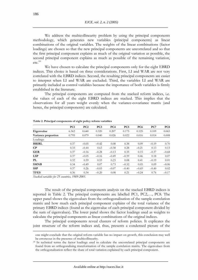

Karsten Staehr Reforms and Economic Growth in Transition Economies
Available online at httpeacesliucit
187
different reform strategies undertaken Some of the principal components have straightforward interpretations while others have less intuitive renditions The growth estimations in the next section reveal that only the following five principal components enter significantly
bull PC1 is broadly the sum of the eight reform indices divided by 3 The
variable can be interpreted as broad-based reforms including liberalisation privatisation and structural measures PC1 captures 795 of total variation in the initial eight reform variables and hence it is not without merit that many studies use an overall reform variable simply calculated as the sum of the EBRD reform indices We refer to PC1 as ldquobroad-based reformsrdquo
bull PC2 has positive factor loadings for price liberalisation market opening and small-scale privatisation It has negative loadings for the rest of the EBRD indices including the numerically large loadings for security markets and competition policy PC2 captures what is sometimes called ldquoearly reformsrdquo or ldquoinitial phase reformsrdquo (EBRD (2002)) ie liberalisation and small-scale privatisation without accompanying structural reforms PC2 is synonymous with ldquoliberalisationrdquo
bull PC6 has large positive loadings for large-scale privatisation and price liberalisation and a numerically large negative loading for small-scale privatisation ie a large PC6 indicates a large extent of large-scale privatisation relative to small-scale privatisation PC6 will be referred to as ldquolarge-scale privatisationrdquo but the principal component could just as well be defined as ldquolack of small-scale privatisationrdquo
bull PC7 is marginally significant in most of the growth regressions PC7 has large positive factors loading for market opening and substantial negative loadings for small-scale privatisation and enterprise restructuring as PC7 captures an early market opening without privatisation or restructuring of production PC7 is referred to as ldquoearly market openingrdquo
bull PC8 has a large positive loading for banking reforms and interest rate liberalisation but a large negative loading for enterprise restructuring PC8 captures a mismatch between banking and enterprise reforms and is referred to as ldquoearly bank liberalisationrdquo
The use of principal components reveals a particular structure of the reform
policies undertaken in transition economies The reform cluster PC1 where liberalisation privatisation and structural reforms are closely synchronised captures 795 of the variation in the EBRD reform indices This high share of variation is explained by the fact that all loadings are positive so PC1 retains the same trend as the underlying EBRD indices
The remaining 205 of variation is explained by PC2 hellip PC8 These principal components denote clusters where liberalisation privatisation and structural reforms do not go hand-in-hand They are examples of combinations of unsynchronised reforms19 This turns out to be useful when exploring the issues of reform complementarity For example PC2 allows us to isolate the effect of liberalisation and small-scale privatisation 19 We avoid use of the term ldquopartial reformsrdquo as it might be confused with the case where the level (or
intensity) of individual reforms is limited
188
EJCE vol 2 n 2 (2005)
Available online at httpeacesliucit
when no other reforms are pursued Similarly PC3 hellip PC8 represent different other clusters of unsynchronised reforms and allow us to consider the effect of these reform patterns
The reform clusters will ndash in different forms ndash be used as right-hand side variables in the growth regressions in following sections This use of principal components to identify clusters of reforms is relatively novel and involves a number of advantages20 It addresses effectively the multicollinearity problem which otherwise obscure inference testing of the importance of individual reform measures and of possible links between the measures
The ldquotraditionalrdquo method of detecting complementarities is to include products of different reform variables together with the reform variables themselves on the right-hand side of the regression (eg Zinne et al 2001) A significant and correctly signed parameter estimate to the multiplicative term is then interpreted as signifying a complementarity between the two reforms This method has several drawbacks First it is essentially a joint test of both a possible complementarity and the specific multiplicative relationship between the two reform variables Second the test has very low power if one or both of the variables displays very little variation Third the multiplicative term could pick up possible non-linearities which are not stemming from reform complementarities Fourth the method has also low power if there are many correlated reform variables If the multiplicative term of two reform variables is significant then the multiplicative term of two other variables strongly correlated with the first two variables will likely also be correlated Fifth the method is generally best suited for cases where there are only few reform variables which have to be interacted
This discussion suggests that the method of using multiplicative terms is less useful in our case with many correlated reform variables We propose instead using the reform clusters identified above as right-hand side variables The eight clusters represent distinct combinations of reforms which are interpretable as policy strategies cf above The weights of the individual reforms in the clusters are determined so that the resulting clusters are uncorrelated implying the clusters represent mutual exclusive reform packages21 The uncorrelated reforms clusters also imply that (linear combinations of) all the EBRD indices can be entered as right-hand side variables in the regression model We do not waste information by having to eliminate variables ex ante because of multicollinearity problems We can instead use a standard general-to-specific method of elimination of insignificant variables when specifying our empirical model
5 Reforms and economic growth performance
We can now regress the annual growth rate G on a set of right-hand variables It is customary to include contemporaneous and one-year lagged variables on the right-hand side To facilitate interpretation we implement this lag structure by including the
20 Ahrens and Meurers (2002) also apply factor analysis to stacked right-hand variables but their purpose
method and data set differ from ours Sachs et al (2000) apply a clustering method and de Melo et al (2001) principal components but in both cases only on data for initial conditions Havrylyshyn and van Rooden (2000) use the principal components method on reform data for a single year
21 Testing for complementarities implies ipso facto a cardinal comparison of variables in this case reform indices Using the standard method of multiplicative terms implies an essentially arbitrary combination of the selected indices while the principal components methodology proposed in this paper weights all reform indices so that the resulting clusters are uncorrelated ie no information need to be wasted in this case
Karsten Staehr Reforms and Economic Growth in Transition Economies
Available online at httpeacesliucit
189
contemporaneous first difference and the variable lagged one-year The first difference of a variable is indicated by a pre-imposed ∆ Employing a general-to-specific methodology we initially enter the following variables on the right-hand side G(ndash1) TREND WAR ∆LI LI(ndash1) ∆PC1 PC1(ndash1) hellip ∆PC8 PC8(ndash1)
The lagged growth rate G(ndash1) the trend variable TREND and the conflict dummy WAR are essentially control variables while the policy interest focuses on the terms involving logarithmic inflation LI and the principal components PC1 hellip PC8 In most cases we allow for country-specific fixed effects and exclude the variables capturing initial conditions INI1 and INI2 from the regression
The highly different growth paths among the countries in the sample may lead to cross-section heteroskedasticity Consequently we perform weighted least squares (WLS) estimation with cross-section weights derived from residual variances from a first-stage OLS estimation
It is important to appreciate the ldquoreduced formrdquo nature of growth regressions for transition economies In the absence of a firm theoretical foundation the exercise merely exposes correlation patterns Regarding their panel data regressions Fischer et al (1996b p 231) write ldquohellip results should be viewed as a way of describing data rather than reflecting deep structural relationsrdquo This makes it important to test the robustness of the results Thus we will later inter alia remove variables change the dynamic structure and split the sample
51 Estimation results
Even with our rich general specification a large number of variables are
significant at the 10 level (ie have numerical t-values around or above 165) the war dummy the inflation variables and one or both terms of principal components 1 2 6 7 and 8 The general-to-specific model selection is implemented by successively eliminating the variable with the numerically lowest t-value to the point where all estimates are significant at the 5 level The resulting regression is shown in column (31) in Table 3
The lagged growth rate and the trend variable are both strongly significant with positive parameters These variables most likely reflect the contribution of omitted variables in the regression However the significant lagged growth rate may also be interpreted as the result of slow adjustment to changes in the right-hand side variables Radulescu and Barlow (2002) discuss possible interpretations of this trend Unsurprisingly the parameter to the conflict dummy is negative and significant The parameters to (log) inflation changes and lagged (log) inflation are precisely estimated and have negative signs
Five principal components and in three cases their first differences survive the simplification procedure The parameter to ∆PC1 is negative while the parameter to PC1(ndash1) is positive Broad-based reforms have a short-term cost in form of lower growth the first year but are beneficial for growth from the second year onwards The parameter to ∆PC2 is negative while it is positive to PC2(ndash1) Liberalisation without accompanying reforms has a negative impact on growth in the very short term but a positive impact in the ldquomedium termrdquo ie from the second year onwards The parameters to ∆PC6 and PC6(ndash1) are both negative suggesting that accelerated large-scale privatisation is bad for growth irrespective time horizon The parameter to the term PC7(ndash1) is negative although only marginally significant Market opening without
190
EJCE vol 2 n 2 (2005)
Available online at httpeacesliucit
supporting reforms appears detrimental to growth Finally the parameter to PC8(ndash1) is also negative indicating that a policy of early bank liberalisation without enterprise reform likely affects growth negatively
Table 3 Panel data estimations of growth determinants
(31) (32) (33) (34) (35) (36)a (37)a (38) (39)
023 019 030 029 029 020 017 023G(ndash1)
(436) (277) (599) (571) (273) (222) (264) (381)033 057 020 054 039 022 049 083 040TREND
(352) (371) (201) (557) (400) (109) (211) (254) (292)ndash636 ndash624 ndash602 ndash806 ndash638 ndash796 ndash482 ndash584 ndash920WAR
(ndash374) (ndash296) (ndash330) (ndash534) (ndash330) (ndash253) (ndash179) (ndash280) (ndash606)ndash229 ndash271 ndash262 ndash237 ndash146 ndash288 ndash281 ndash276∆LI
(ndash497) (ndash361) (ndash552) (ndash432) (ndash188) (ndash471) (ndash608) (ndash475)ndash300 ndash262 ndash197 ndash418 ndash244 ndash126 ndash284 ndash363 ndash426LI(ndash1)
(ndash640) (ndash333) (ndash504) (ndash1049) (ndash489) (ndash105) (ndash269) (ndash610) (ndash691)ndash134 ndash242 ndash168 ndash132 ndash199 ndash213 ndash204 174∆PC1
(ndash302) (ndash281) (ndash351) (ndash360) (ndash202) (ndash205) (ndash459) (174)073 027 135 053 044 073 041 056 004PC1(ndash1)
(415) (083) (762) (271) (274) (190) (083) (180) (007)ndash143 ndash138 ndash191 ndash256 ndash093 ndash132 ndash137 026∆PC2
(ndash246) (ndash118) (ndash304) (ndash521) (ndash062) (ndash113) (ndash208) (035)256 378 328 238 114 485 362 263 109PC2(ndash1)
(472) (470) (751) (417) (379) (328) (334) (350) (125)ndash240 ndash135 ndash210 ndash147 ndash167 ndash149 ndash324 221∆PC6
(ndash300) (ndash089) (ndash253) (ndash182) (ndash108) (ndash108) (ndash393) (202)ndash297 ndash349 ndash047 ndash399 ndash124 ndash391 ndash288 ndash448 218PC6(ndash1)
(ndash291) (ndash203) (ndash059) (ndash399) (ndash151) (ndash149) (ndash162) (ndash306) (140)ndash142 ndash258 ndash217 ndash167 ndash188 ndash434 ndash323 050 ndash441PC7(ndash1)
(ndash205) (ndash198) (ndash304) (ndash236) (ndash272) (ndash217) (ndash164) (065) (ndash502)ndash170 ndash285 ndash133 ndash176 ndash280 ndash322 ndash233 ndash288 ndash343PC8(ndash1)
(ndash257) (ndash193) (ndash196) (ndash244) (ndash360) (ndash127) (ndash123) (ndash326) (ndash480) 1038 Constant
(389) 025 INI1
(085) ndash085 INI2
(ndash247) Method WLS OLS WLS WLS WLS GMM GMM WLS WLSSample 90-01 90-01 90-01 90-01 90-01 91-01 91-01 90-95 96-01No obs 300 300 300 300 300 300 300 150 150R2 069 070 065 067 064 059 052The growth rate G is left-hand variable All estimations except (35) are fixed-effect regressions employing country dummies t-statistics based on White Heteroskedasticity consistent standard errors are given in brackets and italics below parameter estimates a The estimated parameters are found from the differenced model using the Arellano-Bond procedure
The first results are standard for the literature (see also the discussion in section 2) Outbreaks of war and high inflation are bad for growth while overall broad-based
Karsten Staehr Reforms and Economic Growth in Transition Economies
Available online at httpeacesliucit
191
reforms are good for growth The new insights are mainly related to the estimates of the effects of unsynchronised reforms ie the effects of PC2 PC6 PC7 and PC8
52 Robustness
Column (32) in Table 3 presents the estimates obtained using ordinary pooled
least squares (OLS) instead of WLS All signs are retained but the parameter estimate to PC1(ndash1) has fallen and is now insignificant22 The estimated parameters and standard errors to ∆PC6 PC6(ndash1) PC7(ndash1) and PC8(ndash1) have also changed to some extent It seems appropriate whenever possible to use WLS
As discussed above endogeneity problems related to contemporary variables might bias the results We have re-estimated regression (31) without ∆LI ∆PC1 ∆PC2 and ∆PC6 The results reported in (33) show that the parameters to the lagged level of the variables LI(ndash1) PC1(ndash1) PC2(ndash1) PC6(ndash1) PC7(ndash1) and PC8(ndash1) have broadly retained their size and significance In practice the endogeneity problem associated with the variables based on EBRD indices is probably not serious as the indices are scored in the middle of the year when little information about the countryrsquos performance is known
Outliers could influence results unduly particularly the large negative growth rates registered for a number of CIS countries For example output contracted 526 in Armenia in 1992 This partly reflects the war in the country at that time but may also be the result of underreporting We replace the growth rate by the transformation 100G(100ndashG) which dampens the impact of large negative growth rates but has little impact on positive growth rates of ldquonormalrdquo size The findings (not shown) are close to those in column (31) so data points with extreme growth rates do not ldquodriverdquo the results Moreover experiments with transformations of other variables and inclusion of dummies to pick up outliers also show that the results are reasonably robust partly because the equations are estimated using WLS
It is relatively uncommon to include the lagged growth rate on the right-hand side of growth regressions for transition economies23 To ensure that our results do not hinge on this specification G(ndash1) is excluded and the results shown in column (34) The main effect is that the parameter to TREND increases With the exception of the parameter to PC1(ndash1) all other parameters increase somewhat numerically This result is intuitive and the medium-term impacts are broadly the same as before as the dynamic effect from the lagged growth rate is now lacking Removing the trend also has a negligible impact on the results (not shown)
To check the robustness of our results we estimate the growth equation dropping the fixed effect dummies and including instead the two variables capturing initial conditions together with a constant The results in column (35) are close to those in column (31) suggesting that the estimated impact of the reform variables is not a mirage caused by different initial conditions affecting both reform choices and growth results INI2 is significant and has the expected negative sign while INI1 is insignificant
22 The problem of obtaining a precise estimate to PC(ndash1) will reappear in a number of the specifications
used for robustness checks 23 Berg et al (1999) include the lagged growth rate on the right-hand side of the regression but find that it
is insignificant
192
EJCE vol 2 n 2 (2005)
Available online at httpeacesliucit
OLS-based estimation methods can yield biased estimates in dynamic panels due to correlation between the country-specific fixed effects and the error term There is still no consensus on which estimation method to use in this case The often-used Arellano-Bond GMM method first eliminates country-specific effects by differencing the equation and then use lagged values of the level variables as GMM instruments24
However GMM estimation like the Arellano-Bond method gives rise to bias in small samples in particular when right-hand side variables are serially correlated Indeed Judson and Owen (1999) show that in a sample with few cross-sections and a short time horizon the Arellano-Bond method performs no better than the fixed-effect OLS estimator (although better than standard OLS without fixed effects) Other methods are likely to perform better depending on the structure of data Beck and Levine (2004) point out that estimates from the Arellano-Bond method could be strongly biased in small-sample dynamic panels with persistent right-hand side variables Nerlove (2002) argues that the Arellano-Bond method is inappropriate in dynamic panels with a short time dimension and examines the properties of a number of other methods without finding any generally superior estimator 25
As a robustness check we estimate the dynamic model with trend using the Arellano-Bond GMM method In the first case we only instrument the lagged growth rate assuming that the contemporaneous right-hand variables (∆LI ∆PC1 ∆PC2 and ∆PC6) are weakly exogenous The results using the Arellano-Bond one-step method are presented in column (36) Although some changes occur the results in (36) are broadly in line with the results of the WLS estimation in (31) and with the OLS estimation in (33) (Note that the Arellano-Bond procedure implies that the sample is reduced one period)
Column (37) shows the results when the contemporaneous variables (∆LI ∆PC1 ∆PC2 and ∆PC6) are also instrumented using Arelleno-Bond level instruments This should eliminate possible endogeneity biases from the contemporaneous right-hand variables Again the changes are not dramatic
The conclusion is that GMM estimation confirms the qualitative results obtained earlier The estimated standard errors are generally larger for the GMM estimations than for the OLSWLS estimations This problem is to some extent related to the ldquoweak instrument problemrdquo causing the GMM estimators to be inefficient in small samples26 We find as do several other studies that the GMM results are not fundamentally different from least-squares-based methods They may however suffer from inference problems
When the sample is split into two subperiods some instability is revealed The estimation results are shown for 1990-95 in column (310) and for 1996-2001 in column (311) The estimation results for the early subperiod correspond closely to the full sample results with the exception of the estimate to PC7(ndash1) which is positive albeit insignificant For the latter subperiod a number of changes are noteworthy First the 24 Instrumentation is required as the error term of the difference equation is still correlated with the left-
hand side variable 25 This is also reflected in eg Pattillo et al (2002) where dynamic growth models are estimated All results
are presented using four different estimation techniques including GMM 26 The use of the Arellano-Bond method is not rejected There is first-order autocorrelation in the
residuals in the differenced model and the Sargan test does not reject the instruments Nevertheless the presence of serially correlated right-hand variables reduces the efficiency of the level instruments The potential small-sample bias is an argument for avoiding a general-to-specific specification search using GMM
Karsten Staehr Reforms and Economic Growth in Transition Economies
Available online at httpeacesliucit
193
parameters to ∆PC1 and ∆PC2 are now positive although none of the variables are significant at the 5 level The short-term costs of reforms seem at most to be a feature of the early stages of transition Second the estimated parameters to PC1(ndash1) and PC2(ndash1) have dropped substantially However the changes to the parameters to ∆PC1 and ∆PC2 combined with the changes to PC1(ndash1) and PC2(ndash1) imply that the effects of the two reform clusters in the 2-4 years interval are broadly unchanged What has changed is merely the adjustment dynamics Third ∆PC6 and PC6(ndash1) have changed sign while PC7(ndash1) is highly significant in the late period In sum reforms do a better job of explaining growth at the beginning of the reform period than at the end A number of studies reach this conclusion eg Radulescu and Barlow (2002) This is consistent with the view that reforms change the structure of these economies likely increasing the importance of traditional growth factors like physical and human capital accumulation
The estimations reported employ ldquocalendar timerdquo Calendar time ndash as opposed to ldquotransition timerdquo ndash is chosen because it gives the longest possible sample ensures more variation in both right-hand and left-hand variables and simplifies interpretation in certain cases As a robustness check most of the regressions in this paper have been re-estimated using transition time using the correspondence suggested in Berg et al (1999) The results (not shown) are broadly similar to those reported The main difference is that the estimates to ∆PC1 and ∆PC2 although still negative tend not to be significant at conventional levels This result is broadly in line with the above finding that the negative and significant parameters to ∆PC1 and ∆PC2 are derived from the early part of the sample (which is shortened for many countries when transition time is used)27
53 Results and discussion
The broadly similar results obtained from many specifications suggest that
several fairly robust conclusions can be drawn concerning the relationship between reforms and growth in transition countries The control variables offer straightforward interpretations Conflict situations affect growth negatively while the lagged growth rate and a trend always attain positive signs
Inflation and increasing inflation are negatively correlated with growth The contemporaneous effect of inflation changes is negative even in the later half of the sample ie there still appears to be no short-term Phillips curve relationship in the transition economies
We find that broad-based reforms as represented by principal component PC1 are good for growth in the medium term while the short-term effect may be negative at the early stages of reform The parameter to PC1(ndash1) has been estimated to values ranging from 022 to 073 (and 135 in an extremely under-parameterised model) This rather broad interval of estimates is somewhat inconvenient as PC1 captures the overall reform progress and different parameter sizes have different implications for the desirability of reforms28
27 Additional robustness tests can be found in the working paper version of this paper Staehr (2003) 28 The result is however consistent with previous contributions which have found a wide range of
estimated parameter values to a broad index of reforms (see discussion in Radulescu and Barlow 2002) Radulescu and Barlow (2002) use an extreme bounds analysis and show that the sum of the EBRD indices does not enter robustly in their growth regressions ie the parameter and the significance of the
194
EJCE vol 2 n 2 (2005)
Available online at httpeacesliucit
Early reforms in the form of liberalisation and small-scale privatisation have a positive medium-term effect on growth even in the absence of other (mainly structural) reforms Liberalisation and small-scale privatisation have a positive effect on growth even if structural reforms are less advanced The short-term impact of early liberalisation appears to be negative at the early stages of reform
A policy of large-scale privatisation and price liberalisation without small-scale privatisation and market opening has a negative impact on growth The impact is contemporaneous as well as medium-term This result broadly confirms the finding in Zinnes et al (2001) that privatisation without enterprise reforms leads to title change with little restructuring Broadly similar results follow from the meta-analysis in Djankov and Murrell (2002) of approximately 100 empirical studies examining restructuring at the enterprise level Fast privatisation of large firms with insufficient supporting reforms hold back firm restructuring and growth (see also Havrylyshyn 2001) Note however that the result implies rapid small-scale privatisation is beneficial to growth even in the absence of large-scale privatisation and price liberalisation
Early market opening without other reforms like small-scale privatisation and enterprise restructuring also seems detrimental to growth at least in the latter part of transition Figuratively one might imagine foreign competition sweeping away domestic state-owned and unreconstructed producers Crafts (2000) and IMF (1997) discuss preconditions necessary to ensure that market opening and international integration is beneficial to growth Again the reasoning can be reversed a policy of small-scale privatisation and enterprise restructuring appear growth enhancing minus even when not backed by market opening
Finally bank liberalisation without enterprise restructuring has a negative impact on growth especially in the later stages of reform An example of this might be the Czech experience in the mid-1990s when excessive bank lending to non-restructured firms contributed to serious banking sector problems and unsatisfactory growth (see OECD 1998 and 2000) The reverse interpretation is that enterprise restructuring is beneficial even in the absence of bank liberalisation
6 Speed of reforms
The speed at which reforms should be introduced and implemented remains a controversial issue within transition economics The debate also covers sequencing and reform complementary as sequenced reforms may take longer to implement than broad-based reforms This section focuses on the effect on growth of speed per se ie the overall speed with which reforms are implemented29
As noted in section 2 an argument for speedy reform exists when the reform level affects growth positively Fast reforms would put the country on a higher path early on allowing the country to enjoy higher growth for a longer period In this sense all estimations presented in section 5 suggest that broad-based reforms (PC1) or
parameter depend on other variables in the regressions Fidrmuc (2003) also found that it is difficult to estimate the parameter to broad-based reforms precisely
29 The speed of reforms is also important for objectives other than growth eg distribution regional development and medium-term political sustainability These issues cannot be addressed in this framework
Karsten Staehr Reforms and Economic Growth in Transition Economies
Available online at httpeacesliucit
195
liberalisation (PC2) should be implemented rapidly30 However as argued in section 2 we are interested in effects on top of this level effect
Testing directly for speed effects presents two challenges We must specify precise and testable hypotheses and then derive and implement tests of those hypotheses Here we consider two hypotheses First speed effects may affect the level of ldquopainrdquo resulting from reforms in the short term Second the speed of reforms may affect medium-term growth and therefore influence the selection of growth path The short-term hypothesis is examined by testing for possible convexity in the short-term reform costs The medium-term hypothesis is tested by the construction of variables that capture respectively the divergence of the actual reform level from the trend level and indicator variables for a countryrsquos rate of reform
61 Non-linearities in short-term costs
The estimations in section 5 implicitly assumed that short-term reform changes
affect growth rates linearly This assumption implies that the short-term costs of reforms are the same whether reforms are implemented quickly or done piecemeal over several years However possible convexities in the short-term impact would imply ceteris paribus that the level of transition ldquopainrdquo might be lower in a slow reform regime
The search for short-term convexities is narrowed to the first two principal components The starting point for our search for convexities is regression (31) in Table 3 For ease of comparison we repeat this regression in column (41) in Table 4 We test first for possible convexities in the link between ∆PC1 and growth ∆PC1 is replaced by the transformation (137+∆PC1)α where α is the parameter allowing for non-linear effects and 137 is added to ensure that the argument is always positive We perform a grid search by varying α = 01 02 hellip searching for the α-value leading to the parameter estimate with the highest t-value The result is shown in column (42) in Table 4 A similar procedure is performed for ∆PC2 with β varied to give the most precise estimate of (141+∆PC2)β The result appears in column (43)
For the term containing ∆PC1 the t-value was maximised for α = 123 while the t-value for the term containing ∆PC2 was maximised for β = 16 There seems to be a high degree of convexity in the short-term growth costs of broad-based reform and a moderate degree in the liberalisation term
The results are obtained in spite of the test being biased against detecting non-linear effects as only linear variables were used in the specification search Still the test has little power In the specification shown in (42) we have added ∆PC1 as a separate right-hand side variable to ldquocompeterdquo with (137+∆PC1)123
The parameters to both (137+∆PC1)123 and ∆PC1 are negative but insignificant A Wald test cannot reject the joint hypothesis that the parameter to (137+∆PC1)123 is 0 and the parameter to ∆PC1 is ndash229 (as in the original specification) We conclude that although the convex specification yields a slightly more precise parameter estimate the difference is not statistically significant The same holds for the convex specification of ∆PC2
30 Naturally the opposite holds for the unsynchronised reforms of the types captured by PC6 PC7 and
PC8
196
EJCE vol 2 n 2 (2005)
Available online at httpeacesliucit
Table 4 Speed effects in panel data estimations of growth determinants
(41)a (42) (43) (44) (45) (46)
023 026 023 032 027 027G(ndash1)
(436) (498) (436) (553) (549) (568)033 030 033 042 060 070TREND
(352) (342) (352) (271) (541) (643)ndash636 ndash594 ndash642 ndash314 ndash647 ndash633WAR
(ndash374) (ndash387) (ndash381) (ndash155) (ndash330) (ndash319)ndash229 ndash232 ndash222 ndash132 ndash243 ndash243∆LI
(ndash497) (ndash559) (ndash486) (ndash228) (ndash441) (ndash445)ndash300 ndash310 ndash298 ndash219 ndash262 ndash265LI(ndash1)
(ndash640) (ndash741) (ndash642) (ndash324) (ndash518) (ndash536)ndash134 ndash117 ndash001 ndash151 ndash162∆PC1
(ndash302) (ndash254) (ndash002) (ndash420) (ndash502)073 082 073 023 036 039PC1(ndash1)
(415) (496) (412) (053) (232) (276)ndash143 ndash123 142 ndash249 ndash247∆PC2
(ndash246) (ndash206) (193) (ndash511) (ndash551)256 238 246 351 108 080PC2(ndash1)
(472) (488) (450) (454) (350) (260)ndash240 ndash291 ndash241 ndash227 ndash137 ndash142∆PC6
(ndash300) (ndash369) (ndash302 (ndash207) (ndash171) (ndash185)ndash297 ndash312 ndash301 ndash169 ndash128 ndash115PC6(ndash1)
(ndash291) (ndash319) (ndash295) (ndash115) (ndash161) (ndash150)ndash142 ndash121 ndash147 ndash280 ndash187 ndash170PC7(ndash1)
(ndash205) (ndash177) (ndash209) (ndash269) (ndash280) (ndash251)ndash170 ndash116 ndash165 ndash105 ndash217 ndash208PC8(ndash1)
(ndash257) (ndash173) (ndash248) (ndash124) (ndash273) (ndash276) ndash313middot10ndash8 (137 + ∆PC1)123
(ndash436) ndash08 (141 + ∆PC2)16
(ndash262) 012 PC1SP
(062) 1038 1006Constant
(392) (387) 003 INI1
(009) ndash098 INI2
(ndash290) ndash054 YEAR
(ndash414) ndash377FAST
(ndash688) ndash312SLOW
(ndash503)Method WLS WLS WLS WLS WLS WLSSample 90-01 90-01 90-01 93-01 90-01 90-01No observations 300 300 300 225 300 300R2 069 068 069 062 066 066The growth rate G is left-hand variable t-statistics based on White Heteroskedasticity consistent standard errors are given in brackets and italics below parameter estimates a For ease of comparison column (41) repeats column (31) from Table 3
Karsten Staehr Reforms and Economic Growth in Transition Economies
Available online at httpeacesliucit
197
62 Divergence from trend reform path We construct a variable that directly reflects the speed of reforms based on a
suggestion in Berg et al (1999) The idea is to calculate the trend reform level during a fixed time window and then compare the actual reform level with the calculated trend value during the early part of the window The higher the early reform level is above trend level the speedier the implementation of reforms
The implementation speed of broad-based reforms is considered within a four-year window We follow the convention in econometrics and use no time indication of the current realisation of a variable We use τ to indicate years from current year Thus τ = 0 indicates the current year τ = ndash1 indicates a one year lag τ = ndash2 indicates a two year lag etc With this notation the contemporaneous reform level is PC1 and the reform level in year τ ie the reform level lagged τ years is PC1(τ)
We consider a four-year window preceding the current year The total change in the reform index during the four year period is [PC1 ndash PC1(ndash4)] and the average annual change is [PC1 ndash PC1(ndash4)]4 Accordingly the expected trend reform level for any year in the four-year window preceding the current year is
EPC1(τ) = PC1(ndash4) + (4 + τ)middot[PC1 ndash PC1(ndash4)]4 where τ = ndash4 hellip ndash1 For τ = ndash4 EPC1(τ) = PC1(τ) while EPC1(τ) increases
linearly with the annual rate of reform change for τ = ndash3 ndash2 ndash1 The speed variable PC1SP is the sum of the differences between the actual and the trend reform level for years τ = ndash3 and τ = ndash2
PC1SP = [PC1(ndash3) ndash EPC1(ndash3)] + [PC1(ndash2) ndash EPC1(ndash2)] PC1SP is added to specification (31) with the result shown in column (44) in
Table 4 Note that the sample period has changed as PC1SP absorbs three years of the sample The parameter to PC1SP is positive but insignificant31 It should be noted however that the regression contains many variables which could make it difficult for PC1SP to attain significance The partial correlation between G and PC1SP is positive and highly significant Still experiments with different samples non-linear transformations and lagged values of PC1SP show that no stable relationship exists On the suspicion of asymmetric effects we split PC1SP into two variables respectively containing positive and negative values but the results (not shown) were again inconclusive Similar exercises using the liberalisation cluster (PC2) fail to yield any consistent results
63 Scoring of reform speed
Finally we apply methods derived from Wolf (1999) to test for speed effects Initially the number of years from the start of the reform process (ie year 0 using
31 The parameter to ∆PC1 is now insignificant This is the consequence of the shorter sample (also see
(39) in Table 3) and the exclusion of PC1SP
198
EJCE vol 2 n 2 (2005)
Available online at httpeacesliucit
transition time) until PC1 has increased by 4 is counted32 This number (score) would be eg 2 for the Czech Republic and Estonia 4 for Hungary and Moldova and 7 for Bulgaria and Croatia For some countries eg Belarus and Macedonia PC1 does not increase by 4 units within by 2001
The variable YEAR is constructed as follows For 1989-1997 it contains zeros for 1998-2001 it contains the speed score provided the score is less than 8 otherwise zero The construction of YEAR with zeros until 1998 implies that only medium-term effects of the speed score are captured and ensures that the measure of reform speed does not affect growth before reforms are actually implemented33
We include YEAR in regression (35) with a constant term and controls for initial conditions (Fixed effects estimation cannot be used when YEAR is included) The result is shown in column (45) in Table 4 The estimated parameter is negative and significant indicating that reform speed is positively correlated with growth ie rapid reform is associated with higher medium-term growth
Another test separates the transition countries into three groups The first group consists of countries undertaking fast reforms (YEAR le 3) the second group consists of countries undertaking gradual reforms (4 le YEAR le 7) and the third group contains reform-resistant laggards (YEAR ge 8) The dummy FAST has zeros for 1989-97 and ones for 1998-2001 for all countries in the first group The dummy SLOW has zeros for 1989-97 and ones for countries in the second group Column (46) in Table 4 shows the result of adding these two dummy variables to regression (35) Both have negative (and significant) parameters The parameter to FAST is smaller than to SLOW which may indicate that slow reforms were beneficial to growth However the Wald test cannot reject the hypothesis that the two parameters are identical
The method of directly inserting the variables YEAR or FAST and SLOW into the growth regression did not provide firm evidence on the effect of speed However there is no evidence that speedy reforms hampered medium-term growth
64 Discussion
Early reforms allow more years in which the transition country can reap the benefits Beyond this trivial finding the panel data methodology employed in this paper does not provide strong arguments for or against rapid reform The short-term cost of reforms might be larger when implemented in bulk but the effect is small and insignificant The medium-term growth effects of rapid reform are uncertain but rapid reforms appear unlikely to hamper growth In sum the speed of reforms does not appear to a quantitatively substantial impact on growth over and above the level effect This result is in conflict with the conclusions in World Bank (1996) and Berg et al (1999) but is broadly in line with Wolf (1999)
32 For a country starting with all reform indices at their lowest level (eg most countries emerging from
the Soviet Union) an increase of PC1 equal to 4 signifies that the country is halfway to a well-developed market economy
33 It also implies that the variable YEAR only contributes to explaining growth in the last four years of the sample 1990-2001 ie the part of the sample where the other right-hand variables are relative less effective
Karsten Staehr Reforms and Economic Growth in Transition Economies
Available online at httpeacesliucit
199
7 Final comments
A novel feature of this paper was the use of principal component clustering of the EBRD reform indices to infer the structure of reform in transition economies A cluster of synchronised broad-based reforms ie liberalisation privatisation and structural reforms covers 795 of all variation in the initial EBRD reform indices A cluster of liberalisation and small-scale reforms without other reforms explains 79 of the variation while six other clusters of unsynchronised reforms span the remaining 126
The growth regressions included the reform clusters inflation terms and control variables As in most other studies inflation was found to be detrimental to growth Synchronised broad-based reforms had a positive impact on growth in the medium term with a negative short-term effect at the early stages of reform Also a policy of liberalisation and small-scale privatisation without accompanying structural reforms were shown to have a positive effect (again with a possible early negative short-term effect) Accelerated large-scale privatisation without small-scale privatisation and structural reforms were found likely to harm growth both in the short and the medium term
Conversely small-scale privatisation without large-scale privatisation appears beneficial to growth A less certain result is that market opening and price liberalisation without accompanying privatisation and enterprise reforms appear correlated with lower growth but this effect stems primarily for the most recent period Reversing this result privatisation and restructuring without market opening may be good for growth Finally bank liberalisation without enterprise restructuring might be harmful while enterprise reforms without bank liberalisation may increase growth
Effects from the speed of reforms are mostly absent with the exception that early reforms leave the transition country a longer period in which to reap the benefits of reforms Possible negative short-term effects of rapid reforms are likely to be modest and could be balanced by possible positive medium-term effects The broad overall conclusion is that speed per se has no discernible impact on growth
Finally what can we now say about the three questions raised in the introduction
First the analysis revealed a complex pattern of reform complementarities with notable implications for the sequencing of reforms Balanced wide-ranging reforms based on simultaneous progress in liberalisation privatisation and structural reforms are favourable to growth and hence suggest a mutually reinforcing effect of various reform elements
Liberalisation combined with small-scale privatisation is beneficial even in the absence of other reforms In this case unsynchronised reforms produce positive growth effects Thus liberalisation and small-scale privatisation are not perfectly complementary to deeper reforms such as large-scale privatisation and structural reforms A sequenced reform policy that stresses liberalisation and small-scale privatisation is beneficial Early ldquoeasyrdquo reforms should therefore not be postponed in the absence of a comprehensive reform strategy
A number of unsynchronised reform packages proved detrimental to growth Sequenced policy packages involving large-scale privatisation without small-scale privatisation market opening without accompanying reforms and bank liberalisation without enterprise restructuring lead to lower growth in the short andor medium term Conversely a ldquoreversalrdquo of the policy mix would produce packages beneficial to growth
200
EJCE vol 2 n 2 (2005)
Available online at httpeacesliucit
In sum the statistically significant parameters to a number of unsynchronised reform clusters support the view that reforms need to be fine-tuned to take into account complex interactions among reforms
Second we asked which reforms are of foremost importance Within the set of variables used in this paper and using a broad brush a number of variables stand out Inflation stabilisation repeatedly proved important Price liberalisation small-scale privatisation enterprise restructuring (and to a lesser degree trade opening) were generally important in many different combinations with other reforms Large-scale privatisation financial sector reforms and market regulation mainly proved beneficial when they were part of a larger more comprehensive reform packages These results seem to support the view that reform policies are crucial minus even countries that fail to attempt deep structural changes can gain from reforms These findings are broadly in line with the findings in Havrylyshyn and van Rooden (2000) As a caveat we note that only a few variables included in our analysis reflect currently popular themes such as institutional quality and social capital
Third the finding that speed per se is of little importance for growth seems to favour relatively rapid implementation of reforms due to the level effect However this finding also implies there is no direct loss from slowing reforms when it is necessary to get content or sequencing right
These results probably disappoint supporters of big-bang as well as supporters of gradualism as they provide no unequivocal support for either view If it is any consolation to the gradualists reform sequencing appears to be important and reforms should preferably progress synchronously Certain sequenced reform paths are clearly counterproductive Likewise for the big-bang supporters initial phase reforms are beneficial even in the absence of deeper reforms Moreover fast reforms appear generally beneficial Thus there is no clear-cut transition strategy that provides the best results for countries endeavouring to convert a centrally planned economy into a market economy There are only policy choices minus some better than others minus and certain strategies that should be avoided
References
Ahrens J Meurers M (2002) lsquoHow Governance Affects the Quality of Policy Reform and Economic Performance New Evidence for Economies in Transitionrsquo Journal for Institutional Innovation Development and Transition 6 35-56
Aslund A (2002) Building Capitalism The Transformation of the Former Soviet Bloc Cambridge University Press Cambridge
Aziz J Wescott R (1997) lsquoPolicy Complementarities and the Washington Consensusrsquo IMF Working Paper No118
Beck T Levine R (2004) lsquoStock Markets Banks and Growth Panel Evidencersquo Journal of Banking and Finance 28 423-442
Berg A Borensztein E Sahay R Zettelmeyer J (1999) lsquoThe Evolution of Output in the Transition Economies Explaining the Differencesrsquo IMF Working Paper No73
Blanchard O Dornbusch R Krugman P Layard R Summers L (1991) Reform in Eastern Europe MIT Press Cambridge MA
Campos N Coricelli F (2002) lsquoGrowth in Transition What We Know What We Donrsquot and What We Shouldrsquo Journal of Economic Literature 90 793-836
Karsten Staehr Reforms and Economic Growth in Transition Economies
Available online at httpeacesliucit
201
Correa R (2002) lsquoThe Washington Consensus in Latin America A Quantitative Evaluationrsquo mimeo San Francisco de Quito University Ecuador
Crafts N (2000) lsquoGlobalization and Growth in the Twentieth Centuryrsquo in Prasad E (ed) Supporting Studies for the World Economic Outlook International Monetary Fund Washington DC
de Melo M Denizer C Gelb A (1997) lsquoFrom Plan to Market Patterns of Transitionrsquo in Blejer M Skreb M (eds) Macroeconomic Stabilization in Transition Economies Cambridge University Press Cambridge
de Melo M Denizer C Gelb A (2001) lsquoCircumstance and Choice The Role of Initial Conditions and Policies in Transition Economiesrsquo World Bank Economic Review 15 1-31
Djankov S Murrell P (2002) lsquoEnterprise Restructuring in Transition A Quantitative Surveyrsquo Journal of Economic Literature 90 739-792
EBRD (1999-2004) Transition Report European Bank for Reconstruction and Development Fidrmuc J (2003) lsquoEconomic Reform Democracy and Growth during Post Communist
Transitionrsquo European Journal of Political Economy 19 583-604 Fischer S Gelb A (1991) lsquoThe Process of Socialist Economic Transformationrsquo Journal of
Economic Perspectives 5 91-105 Fischer S Sahay R (2000) lsquoThe Transition Economies After Ten Yearsrsquo IMF Working Paper
No30 Fischer S Sahay R Vegh C (1996a) lsquoStabilization and Growth in Transition Economies The
Early Experiencersquo Journal of Economic Perspectives 10 45-66 Fischer S Sahay R Vegh C (1996b) lsquoEconomies in Transition The Beginnings of Growthrsquo
American Economic Review 86 229-233 Havrylyshyn O van Rooden R (2000) lsquoInstitutions Matter in Transition but so do Policiesrsquo
IMF Working Paper No70 Havrylyshyn O (2001) lsquoRecovery and Growth in Transition A Decade of Evidencersquo IMF Staff
Paper 48 53-87 Havrylyshyn O Izvorski I van Rooden R (1998) lsquoRecovery and Growth in Transition
Economies 1990-97 A Stylized Regression Analysisrsquo IMF Working Paper No141 Heybey B Murrell P (1999) lsquoThe Relationship Between Economic Growth and the Speed of
Liberalization During the Transitionrsquo Policy Reform 3 121-37 IMF (1997) World Economic Outlook Globalization Opportunities and Challenges May chapter IV IMF (2000) World Economic Outlook Focus on Transition Economies October chapter III Judson R Owen A (1999) lsquoEstimating Dynamic Panel Data Models A Practical Guide for
Macroeconomistsrsquo Economics Letters 65 9-15 Nerlove M (2002) lsquoProperties of Alternative Estimators of Dynamic Panel Models An
Empirical Analysis of Cross-Country Data for the Study of Economic Growthrsquo in Nerlove M Essays in Panel Data Econometrics Cambridge University Press Cambridge
Nsouli S Rached M Funke N (2002) lsquoThe Speed of Adjustment and the Sequencing of Economic Reforms Issues and Guidelines for Policymakersrsquo IMF Working Paper No132
OECD (1998) OECD Economic Surveys Czech Republic May OECD OECD (2000) OECD Economic Surveys Czech Republic February OECD Pattillo C Poirson H Ricca L (2002) lsquoExternal Debt and Growthrsquo IMF Working Paper No69 Radulescu R Barlow D (2002) lsquoThe Relation between Policies and Growth in Transition
Countriesrsquo Economics of Transition 10 719-745 Roland G (2001) lsquoTen Years After hellip Transition and Economicsrsquo IMF Staff Papers 48 29-52
202
EJCE vol 2 n 2 (2005)
Available online at httpeacesliucit
Sachs J Zinnes G Eilat Y (2000) lsquoPatterns of Economic Reform and its Determinants in Transition Economies 1990-1998rsquo Harvard Institute for International Development CAER II Discussion Paper No 61
Staehr K (2003) lsquoReforms and Economic Growth in Transition Economies Complementarity Sequencing and Speedrsquo BOFIT Discussion Paper No1
Stiglitz J (2001) lsquoWhither Reform Ten Years of Transitionrsquo in Pleskovic B Stiglitz J (eds) World Bank Annual Bank Conference on Development Economics 1999 World Bank Washington DC
Wacziarg R (2002) lsquoReview of Easterlyrsquos The Elusive Quest for Growthrsquo Journal of Economic Literature 90 907-918
Wolf H (1999) lsquoTransition Strategies Choices and Outcomesrsquo Princeton Studies in International Finance No85
World Bank (1996) World Development Report 1996 From Plan to Market World Bank Washington DC
World Bank (2002) Transition The First Ten Years Analysis and Lessons for Eastern Europe and the former Soviet Union World Bank Washington DC
Zinnes C Eilat Y Sachs J (2001) lsquoThe Gains from Privatization in Transition Economies Is lsquoChange of Ownershiprsquo Enoughrsquo IMF Staff Papers 48 146-169

Karsten Staehr Reforms and Economic Growth in Transition Economies
Available online at httpeacesliucit
189
contemporaneous first difference and the variable lagged one-year The first difference of a variable is indicated by a pre-imposed ∆ Employing a general-to-specific methodology we initially enter the following variables on the right-hand side G(ndash1) TREND WAR ∆LI LI(ndash1) ∆PC1 PC1(ndash1) hellip ∆PC8 PC8(ndash1)
The lagged growth rate G(ndash1) the trend variable TREND and the conflict dummy WAR are essentially control variables while the policy interest focuses on the terms involving logarithmic inflation LI and the principal components PC1 hellip PC8 In most cases we allow for country-specific fixed effects and exclude the variables capturing initial conditions INI1 and INI2 from the regression
The highly different growth paths among the countries in the sample may lead to cross-section heteroskedasticity Consequently we perform weighted least squares (WLS) estimation with cross-section weights derived from residual variances from a first-stage OLS estimation
It is important to appreciate the ldquoreduced formrdquo nature of growth regressions for transition economies In the absence of a firm theoretical foundation the exercise merely exposes correlation patterns Regarding their panel data regressions Fischer et al (1996b p 231) write ldquohellip results should be viewed as a way of describing data rather than reflecting deep structural relationsrdquo This makes it important to test the robustness of the results Thus we will later inter alia remove variables change the dynamic structure and split the sample
51 Estimation results
Even with our rich general specification a large number of variables are
significant at the 10 level (ie have numerical t-values around or above 165) the war dummy the inflation variables and one or both terms of principal components 1 2 6 7 and 8 The general-to-specific model selection is implemented by successively eliminating the variable with the numerically lowest t-value to the point where all estimates are significant at the 5 level The resulting regression is shown in column (31) in Table 3
The lagged growth rate and the trend variable are both strongly significant with positive parameters These variables most likely reflect the contribution of omitted variables in the regression However the significant lagged growth rate may also be interpreted as the result of slow adjustment to changes in the right-hand side variables Radulescu and Barlow (2002) discuss possible interpretations of this trend Unsurprisingly the parameter to the conflict dummy is negative and significant The parameters to (log) inflation changes and lagged (log) inflation are precisely estimated and have negative signs
Five principal components and in three cases their first differences survive the simplification procedure The parameter to ∆PC1 is negative while the parameter to PC1(ndash1) is positive Broad-based reforms have a short-term cost in form of lower growth the first year but are beneficial for growth from the second year onwards The parameter to ∆PC2 is negative while it is positive to PC2(ndash1) Liberalisation without accompanying reforms has a negative impact on growth in the very short term but a positive impact in the ldquomedium termrdquo ie from the second year onwards The parameters to ∆PC6 and PC6(ndash1) are both negative suggesting that accelerated large-scale privatisation is bad for growth irrespective time horizon The parameter to the term PC7(ndash1) is negative although only marginally significant Market opening without
190
EJCE vol 2 n 2 (2005)
Available online at httpeacesliucit
supporting reforms appears detrimental to growth Finally the parameter to PC8(ndash1) is also negative indicating that a policy of early bank liberalisation without enterprise reform likely affects growth negatively
Table 3 Panel data estimations of growth determinants
(31) (32) (33) (34) (35) (36)a (37)a (38) (39)
023 019 030 029 029 020 017 023G(ndash1)
(436) (277) (599) (571) (273) (222) (264) (381)033 057 020 054 039 022 049 083 040TREND
(352) (371) (201) (557) (400) (109) (211) (254) (292)ndash636 ndash624 ndash602 ndash806 ndash638 ndash796 ndash482 ndash584 ndash920WAR
(ndash374) (ndash296) (ndash330) (ndash534) (ndash330) (ndash253) (ndash179) (ndash280) (ndash606)ndash229 ndash271 ndash262 ndash237 ndash146 ndash288 ndash281 ndash276∆LI
(ndash497) (ndash361) (ndash552) (ndash432) (ndash188) (ndash471) (ndash608) (ndash475)ndash300 ndash262 ndash197 ndash418 ndash244 ndash126 ndash284 ndash363 ndash426LI(ndash1)
(ndash640) (ndash333) (ndash504) (ndash1049) (ndash489) (ndash105) (ndash269) (ndash610) (ndash691)ndash134 ndash242 ndash168 ndash132 ndash199 ndash213 ndash204 174∆PC1
(ndash302) (ndash281) (ndash351) (ndash360) (ndash202) (ndash205) (ndash459) (174)073 027 135 053 044 073 041 056 004PC1(ndash1)
(415) (083) (762) (271) (274) (190) (083) (180) (007)ndash143 ndash138 ndash191 ndash256 ndash093 ndash132 ndash137 026∆PC2
(ndash246) (ndash118) (ndash304) (ndash521) (ndash062) (ndash113) (ndash208) (035)256 378 328 238 114 485 362 263 109PC2(ndash1)
(472) (470) (751) (417) (379) (328) (334) (350) (125)ndash240 ndash135 ndash210 ndash147 ndash167 ndash149 ndash324 221∆PC6
(ndash300) (ndash089) (ndash253) (ndash182) (ndash108) (ndash108) (ndash393) (202)ndash297 ndash349 ndash047 ndash399 ndash124 ndash391 ndash288 ndash448 218PC6(ndash1)
(ndash291) (ndash203) (ndash059) (ndash399) (ndash151) (ndash149) (ndash162) (ndash306) (140)ndash142 ndash258 ndash217 ndash167 ndash188 ndash434 ndash323 050 ndash441PC7(ndash1)
(ndash205) (ndash198) (ndash304) (ndash236) (ndash272) (ndash217) (ndash164) (065) (ndash502)ndash170 ndash285 ndash133 ndash176 ndash280 ndash322 ndash233 ndash288 ndash343PC8(ndash1)
(ndash257) (ndash193) (ndash196) (ndash244) (ndash360) (ndash127) (ndash123) (ndash326) (ndash480) 1038 Constant
(389) 025 INI1
(085) ndash085 INI2
(ndash247) Method WLS OLS WLS WLS WLS GMM GMM WLS WLSSample 90-01 90-01 90-01 90-01 90-01 91-01 91-01 90-95 96-01No obs 300 300 300 300 300 300 300 150 150R2 069 070 065 067 064 059 052The growth rate G is left-hand variable All estimations except (35) are fixed-effect regressions employing country dummies t-statistics based on White Heteroskedasticity consistent standard errors are given in brackets and italics below parameter estimates a The estimated parameters are found from the differenced model using the Arellano-Bond procedure
The first results are standard for the literature (see also the discussion in section 2) Outbreaks of war and high inflation are bad for growth while overall broad-based
Karsten Staehr Reforms and Economic Growth in Transition Economies
Available online at httpeacesliucit
191
reforms are good for growth The new insights are mainly related to the estimates of the effects of unsynchronised reforms ie the effects of PC2 PC6 PC7 and PC8
52 Robustness
Column (32) in Table 3 presents the estimates obtained using ordinary pooled
least squares (OLS) instead of WLS All signs are retained but the parameter estimate to PC1(ndash1) has fallen and is now insignificant22 The estimated parameters and standard errors to ∆PC6 PC6(ndash1) PC7(ndash1) and PC8(ndash1) have also changed to some extent It seems appropriate whenever possible to use WLS
As discussed above endogeneity problems related to contemporary variables might bias the results We have re-estimated regression (31) without ∆LI ∆PC1 ∆PC2 and ∆PC6 The results reported in (33) show that the parameters to the lagged level of the variables LI(ndash1) PC1(ndash1) PC2(ndash1) PC6(ndash1) PC7(ndash1) and PC8(ndash1) have broadly retained their size and significance In practice the endogeneity problem associated with the variables based on EBRD indices is probably not serious as the indices are scored in the middle of the year when little information about the countryrsquos performance is known
Outliers could influence results unduly particularly the large negative growth rates registered for a number of CIS countries For example output contracted 526 in Armenia in 1992 This partly reflects the war in the country at that time but may also be the result of underreporting We replace the growth rate by the transformation 100G(100ndashG) which dampens the impact of large negative growth rates but has little impact on positive growth rates of ldquonormalrdquo size The findings (not shown) are close to those in column (31) so data points with extreme growth rates do not ldquodriverdquo the results Moreover experiments with transformations of other variables and inclusion of dummies to pick up outliers also show that the results are reasonably robust partly because the equations are estimated using WLS
It is relatively uncommon to include the lagged growth rate on the right-hand side of growth regressions for transition economies23 To ensure that our results do not hinge on this specification G(ndash1) is excluded and the results shown in column (34) The main effect is that the parameter to TREND increases With the exception of the parameter to PC1(ndash1) all other parameters increase somewhat numerically This result is intuitive and the medium-term impacts are broadly the same as before as the dynamic effect from the lagged growth rate is now lacking Removing the trend also has a negligible impact on the results (not shown)
To check the robustness of our results we estimate the growth equation dropping the fixed effect dummies and including instead the two variables capturing initial conditions together with a constant The results in column (35) are close to those in column (31) suggesting that the estimated impact of the reform variables is not a mirage caused by different initial conditions affecting both reform choices and growth results INI2 is significant and has the expected negative sign while INI1 is insignificant
22 The problem of obtaining a precise estimate to PC(ndash1) will reappear in a number of the specifications
used for robustness checks 23 Berg et al (1999) include the lagged growth rate on the right-hand side of the regression but find that it
is insignificant
192
EJCE vol 2 n 2 (2005)
Available online at httpeacesliucit
OLS-based estimation methods can yield biased estimates in dynamic panels due to correlation between the country-specific fixed effects and the error term There is still no consensus on which estimation method to use in this case The often-used Arellano-Bond GMM method first eliminates country-specific effects by differencing the equation and then use lagged values of the level variables as GMM instruments24
However GMM estimation like the Arellano-Bond method gives rise to bias in small samples in particular when right-hand side variables are serially correlated Indeed Judson and Owen (1999) show that in a sample with few cross-sections and a short time horizon the Arellano-Bond method performs no better than the fixed-effect OLS estimator (although better than standard OLS without fixed effects) Other methods are likely to perform better depending on the structure of data Beck and Levine (2004) point out that estimates from the Arellano-Bond method could be strongly biased in small-sample dynamic panels with persistent right-hand side variables Nerlove (2002) argues that the Arellano-Bond method is inappropriate in dynamic panels with a short time dimension and examines the properties of a number of other methods without finding any generally superior estimator 25
As a robustness check we estimate the dynamic model with trend using the Arellano-Bond GMM method In the first case we only instrument the lagged growth rate assuming that the contemporaneous right-hand variables (∆LI ∆PC1 ∆PC2 and ∆PC6) are weakly exogenous The results using the Arellano-Bond one-step method are presented in column (36) Although some changes occur the results in (36) are broadly in line with the results of the WLS estimation in (31) and with the OLS estimation in (33) (Note that the Arellano-Bond procedure implies that the sample is reduced one period)
Column (37) shows the results when the contemporaneous variables (∆LI ∆PC1 ∆PC2 and ∆PC6) are also instrumented using Arelleno-Bond level instruments This should eliminate possible endogeneity biases from the contemporaneous right-hand variables Again the changes are not dramatic
The conclusion is that GMM estimation confirms the qualitative results obtained earlier The estimated standard errors are generally larger for the GMM estimations than for the OLSWLS estimations This problem is to some extent related to the ldquoweak instrument problemrdquo causing the GMM estimators to be inefficient in small samples26 We find as do several other studies that the GMM results are not fundamentally different from least-squares-based methods They may however suffer from inference problems
When the sample is split into two subperiods some instability is revealed The estimation results are shown for 1990-95 in column (310) and for 1996-2001 in column (311) The estimation results for the early subperiod correspond closely to the full sample results with the exception of the estimate to PC7(ndash1) which is positive albeit insignificant For the latter subperiod a number of changes are noteworthy First the 24 Instrumentation is required as the error term of the difference equation is still correlated with the left-
hand side variable 25 This is also reflected in eg Pattillo et al (2002) where dynamic growth models are estimated All results
are presented using four different estimation techniques including GMM 26 The use of the Arellano-Bond method is not rejected There is first-order autocorrelation in the
residuals in the differenced model and the Sargan test does not reject the instruments Nevertheless the presence of serially correlated right-hand variables reduces the efficiency of the level instruments The potential small-sample bias is an argument for avoiding a general-to-specific specification search using GMM
Karsten Staehr Reforms and Economic Growth in Transition Economies
Available online at httpeacesliucit
193
parameters to ∆PC1 and ∆PC2 are now positive although none of the variables are significant at the 5 level The short-term costs of reforms seem at most to be a feature of the early stages of transition Second the estimated parameters to PC1(ndash1) and PC2(ndash1) have dropped substantially However the changes to the parameters to ∆PC1 and ∆PC2 combined with the changes to PC1(ndash1) and PC2(ndash1) imply that the effects of the two reform clusters in the 2-4 years interval are broadly unchanged What has changed is merely the adjustment dynamics Third ∆PC6 and PC6(ndash1) have changed sign while PC7(ndash1) is highly significant in the late period In sum reforms do a better job of explaining growth at the beginning of the reform period than at the end A number of studies reach this conclusion eg Radulescu and Barlow (2002) This is consistent with the view that reforms change the structure of these economies likely increasing the importance of traditional growth factors like physical and human capital accumulation
The estimations reported employ ldquocalendar timerdquo Calendar time ndash as opposed to ldquotransition timerdquo ndash is chosen because it gives the longest possible sample ensures more variation in both right-hand and left-hand variables and simplifies interpretation in certain cases As a robustness check most of the regressions in this paper have been re-estimated using transition time using the correspondence suggested in Berg et al (1999) The results (not shown) are broadly similar to those reported The main difference is that the estimates to ∆PC1 and ∆PC2 although still negative tend not to be significant at conventional levels This result is broadly in line with the above finding that the negative and significant parameters to ∆PC1 and ∆PC2 are derived from the early part of the sample (which is shortened for many countries when transition time is used)27
53 Results and discussion
The broadly similar results obtained from many specifications suggest that
several fairly robust conclusions can be drawn concerning the relationship between reforms and growth in transition countries The control variables offer straightforward interpretations Conflict situations affect growth negatively while the lagged growth rate and a trend always attain positive signs
Inflation and increasing inflation are negatively correlated with growth The contemporaneous effect of inflation changes is negative even in the later half of the sample ie there still appears to be no short-term Phillips curve relationship in the transition economies
We find that broad-based reforms as represented by principal component PC1 are good for growth in the medium term while the short-term effect may be negative at the early stages of reform The parameter to PC1(ndash1) has been estimated to values ranging from 022 to 073 (and 135 in an extremely under-parameterised model) This rather broad interval of estimates is somewhat inconvenient as PC1 captures the overall reform progress and different parameter sizes have different implications for the desirability of reforms28
27 Additional robustness tests can be found in the working paper version of this paper Staehr (2003) 28 The result is however consistent with previous contributions which have found a wide range of
estimated parameter values to a broad index of reforms (see discussion in Radulescu and Barlow 2002) Radulescu and Barlow (2002) use an extreme bounds analysis and show that the sum of the EBRD indices does not enter robustly in their growth regressions ie the parameter and the significance of the
194
EJCE vol 2 n 2 (2005)
Available online at httpeacesliucit
Early reforms in the form of liberalisation and small-scale privatisation have a positive medium-term effect on growth even in the absence of other (mainly structural) reforms Liberalisation and small-scale privatisation have a positive effect on growth even if structural reforms are less advanced The short-term impact of early liberalisation appears to be negative at the early stages of reform
A policy of large-scale privatisation and price liberalisation without small-scale privatisation and market opening has a negative impact on growth The impact is contemporaneous as well as medium-term This result broadly confirms the finding in Zinnes et al (2001) that privatisation without enterprise reforms leads to title change with little restructuring Broadly similar results follow from the meta-analysis in Djankov and Murrell (2002) of approximately 100 empirical studies examining restructuring at the enterprise level Fast privatisation of large firms with insufficient supporting reforms hold back firm restructuring and growth (see also Havrylyshyn 2001) Note however that the result implies rapid small-scale privatisation is beneficial to growth even in the absence of large-scale privatisation and price liberalisation
Early market opening without other reforms like small-scale privatisation and enterprise restructuring also seems detrimental to growth at least in the latter part of transition Figuratively one might imagine foreign competition sweeping away domestic state-owned and unreconstructed producers Crafts (2000) and IMF (1997) discuss preconditions necessary to ensure that market opening and international integration is beneficial to growth Again the reasoning can be reversed a policy of small-scale privatisation and enterprise restructuring appear growth enhancing minus even when not backed by market opening
Finally bank liberalisation without enterprise restructuring has a negative impact on growth especially in the later stages of reform An example of this might be the Czech experience in the mid-1990s when excessive bank lending to non-restructured firms contributed to serious banking sector problems and unsatisfactory growth (see OECD 1998 and 2000) The reverse interpretation is that enterprise restructuring is beneficial even in the absence of bank liberalisation
6 Speed of reforms
The speed at which reforms should be introduced and implemented remains a controversial issue within transition economics The debate also covers sequencing and reform complementary as sequenced reforms may take longer to implement than broad-based reforms This section focuses on the effect on growth of speed per se ie the overall speed with which reforms are implemented29
As noted in section 2 an argument for speedy reform exists when the reform level affects growth positively Fast reforms would put the country on a higher path early on allowing the country to enjoy higher growth for a longer period In this sense all estimations presented in section 5 suggest that broad-based reforms (PC1) or
parameter depend on other variables in the regressions Fidrmuc (2003) also found that it is difficult to estimate the parameter to broad-based reforms precisely
29 The speed of reforms is also important for objectives other than growth eg distribution regional development and medium-term political sustainability These issues cannot be addressed in this framework
Karsten Staehr Reforms and Economic Growth in Transition Economies
Available online at httpeacesliucit
195
liberalisation (PC2) should be implemented rapidly30 However as argued in section 2 we are interested in effects on top of this level effect
Testing directly for speed effects presents two challenges We must specify precise and testable hypotheses and then derive and implement tests of those hypotheses Here we consider two hypotheses First speed effects may affect the level of ldquopainrdquo resulting from reforms in the short term Second the speed of reforms may affect medium-term growth and therefore influence the selection of growth path The short-term hypothesis is examined by testing for possible convexity in the short-term reform costs The medium-term hypothesis is tested by the construction of variables that capture respectively the divergence of the actual reform level from the trend level and indicator variables for a countryrsquos rate of reform
61 Non-linearities in short-term costs
The estimations in section 5 implicitly assumed that short-term reform changes
affect growth rates linearly This assumption implies that the short-term costs of reforms are the same whether reforms are implemented quickly or done piecemeal over several years However possible convexities in the short-term impact would imply ceteris paribus that the level of transition ldquopainrdquo might be lower in a slow reform regime
The search for short-term convexities is narrowed to the first two principal components The starting point for our search for convexities is regression (31) in Table 3 For ease of comparison we repeat this regression in column (41) in Table 4 We test first for possible convexities in the link between ∆PC1 and growth ∆PC1 is replaced by the transformation (137+∆PC1)α where α is the parameter allowing for non-linear effects and 137 is added to ensure that the argument is always positive We perform a grid search by varying α = 01 02 hellip searching for the α-value leading to the parameter estimate with the highest t-value The result is shown in column (42) in Table 4 A similar procedure is performed for ∆PC2 with β varied to give the most precise estimate of (141+∆PC2)β The result appears in column (43)
For the term containing ∆PC1 the t-value was maximised for α = 123 while the t-value for the term containing ∆PC2 was maximised for β = 16 There seems to be a high degree of convexity in the short-term growth costs of broad-based reform and a moderate degree in the liberalisation term
The results are obtained in spite of the test being biased against detecting non-linear effects as only linear variables were used in the specification search Still the test has little power In the specification shown in (42) we have added ∆PC1 as a separate right-hand side variable to ldquocompeterdquo with (137+∆PC1)123
The parameters to both (137+∆PC1)123 and ∆PC1 are negative but insignificant A Wald test cannot reject the joint hypothesis that the parameter to (137+∆PC1)123 is 0 and the parameter to ∆PC1 is ndash229 (as in the original specification) We conclude that although the convex specification yields a slightly more precise parameter estimate the difference is not statistically significant The same holds for the convex specification of ∆PC2
30 Naturally the opposite holds for the unsynchronised reforms of the types captured by PC6 PC7 and
PC8
196
EJCE vol 2 n 2 (2005)
Available online at httpeacesliucit
Table 4 Speed effects in panel data estimations of growth determinants
(41)a (42) (43) (44) (45) (46)
023 026 023 032 027 027G(ndash1)
(436) (498) (436) (553) (549) (568)033 030 033 042 060 070TREND
(352) (342) (352) (271) (541) (643)ndash636 ndash594 ndash642 ndash314 ndash647 ndash633WAR
(ndash374) (ndash387) (ndash381) (ndash155) (ndash330) (ndash319)ndash229 ndash232 ndash222 ndash132 ndash243 ndash243∆LI
(ndash497) (ndash559) (ndash486) (ndash228) (ndash441) (ndash445)ndash300 ndash310 ndash298 ndash219 ndash262 ndash265LI(ndash1)
(ndash640) (ndash741) (ndash642) (ndash324) (ndash518) (ndash536)ndash134 ndash117 ndash001 ndash151 ndash162∆PC1
(ndash302) (ndash254) (ndash002) (ndash420) (ndash502)073 082 073 023 036 039PC1(ndash1)
(415) (496) (412) (053) (232) (276)ndash143 ndash123 142 ndash249 ndash247∆PC2
(ndash246) (ndash206) (193) (ndash511) (ndash551)256 238 246 351 108 080PC2(ndash1)
(472) (488) (450) (454) (350) (260)ndash240 ndash291 ndash241 ndash227 ndash137 ndash142∆PC6
(ndash300) (ndash369) (ndash302 (ndash207) (ndash171) (ndash185)ndash297 ndash312 ndash301 ndash169 ndash128 ndash115PC6(ndash1)
(ndash291) (ndash319) (ndash295) (ndash115) (ndash161) (ndash150)ndash142 ndash121 ndash147 ndash280 ndash187 ndash170PC7(ndash1)
(ndash205) (ndash177) (ndash209) (ndash269) (ndash280) (ndash251)ndash170 ndash116 ndash165 ndash105 ndash217 ndash208PC8(ndash1)
(ndash257) (ndash173) (ndash248) (ndash124) (ndash273) (ndash276) ndash313middot10ndash8 (137 + ∆PC1)123
(ndash436) ndash08 (141 + ∆PC2)16
(ndash262) 012 PC1SP
(062) 1038 1006Constant
(392) (387) 003 INI1
(009) ndash098 INI2
(ndash290) ndash054 YEAR
(ndash414) ndash377FAST
(ndash688) ndash312SLOW
(ndash503)Method WLS WLS WLS WLS WLS WLSSample 90-01 90-01 90-01 93-01 90-01 90-01No observations 300 300 300 225 300 300R2 069 068 069 062 066 066The growth rate G is left-hand variable t-statistics based on White Heteroskedasticity consistent standard errors are given in brackets and italics below parameter estimates a For ease of comparison column (41) repeats column (31) from Table 3
Karsten Staehr Reforms and Economic Growth in Transition Economies
Available online at httpeacesliucit
197
62 Divergence from trend reform path We construct a variable that directly reflects the speed of reforms based on a
suggestion in Berg et al (1999) The idea is to calculate the trend reform level during a fixed time window and then compare the actual reform level with the calculated trend value during the early part of the window The higher the early reform level is above trend level the speedier the implementation of reforms
The implementation speed of broad-based reforms is considered within a four-year window We follow the convention in econometrics and use no time indication of the current realisation of a variable We use τ to indicate years from current year Thus τ = 0 indicates the current year τ = ndash1 indicates a one year lag τ = ndash2 indicates a two year lag etc With this notation the contemporaneous reform level is PC1 and the reform level in year τ ie the reform level lagged τ years is PC1(τ)
We consider a four-year window preceding the current year The total change in the reform index during the four year period is [PC1 ndash PC1(ndash4)] and the average annual change is [PC1 ndash PC1(ndash4)]4 Accordingly the expected trend reform level for any year in the four-year window preceding the current year is
EPC1(τ) = PC1(ndash4) + (4 + τ)middot[PC1 ndash PC1(ndash4)]4 where τ = ndash4 hellip ndash1 For τ = ndash4 EPC1(τ) = PC1(τ) while EPC1(τ) increases
linearly with the annual rate of reform change for τ = ndash3 ndash2 ndash1 The speed variable PC1SP is the sum of the differences between the actual and the trend reform level for years τ = ndash3 and τ = ndash2
PC1SP = [PC1(ndash3) ndash EPC1(ndash3)] + [PC1(ndash2) ndash EPC1(ndash2)] PC1SP is added to specification (31) with the result shown in column (44) in
Table 4 Note that the sample period has changed as PC1SP absorbs three years of the sample The parameter to PC1SP is positive but insignificant31 It should be noted however that the regression contains many variables which could make it difficult for PC1SP to attain significance The partial correlation between G and PC1SP is positive and highly significant Still experiments with different samples non-linear transformations and lagged values of PC1SP show that no stable relationship exists On the suspicion of asymmetric effects we split PC1SP into two variables respectively containing positive and negative values but the results (not shown) were again inconclusive Similar exercises using the liberalisation cluster (PC2) fail to yield any consistent results
63 Scoring of reform speed
Finally we apply methods derived from Wolf (1999) to test for speed effects Initially the number of years from the start of the reform process (ie year 0 using
31 The parameter to ∆PC1 is now insignificant This is the consequence of the shorter sample (also see
(39) in Table 3) and the exclusion of PC1SP
198
EJCE vol 2 n 2 (2005)
Available online at httpeacesliucit
transition time) until PC1 has increased by 4 is counted32 This number (score) would be eg 2 for the Czech Republic and Estonia 4 for Hungary and Moldova and 7 for Bulgaria and Croatia For some countries eg Belarus and Macedonia PC1 does not increase by 4 units within by 2001
The variable YEAR is constructed as follows For 1989-1997 it contains zeros for 1998-2001 it contains the speed score provided the score is less than 8 otherwise zero The construction of YEAR with zeros until 1998 implies that only medium-term effects of the speed score are captured and ensures that the measure of reform speed does not affect growth before reforms are actually implemented33
We include YEAR in regression (35) with a constant term and controls for initial conditions (Fixed effects estimation cannot be used when YEAR is included) The result is shown in column (45) in Table 4 The estimated parameter is negative and significant indicating that reform speed is positively correlated with growth ie rapid reform is associated with higher medium-term growth
Another test separates the transition countries into three groups The first group consists of countries undertaking fast reforms (YEAR le 3) the second group consists of countries undertaking gradual reforms (4 le YEAR le 7) and the third group contains reform-resistant laggards (YEAR ge 8) The dummy FAST has zeros for 1989-97 and ones for 1998-2001 for all countries in the first group The dummy SLOW has zeros for 1989-97 and ones for countries in the second group Column (46) in Table 4 shows the result of adding these two dummy variables to regression (35) Both have negative (and significant) parameters The parameter to FAST is smaller than to SLOW which may indicate that slow reforms were beneficial to growth However the Wald test cannot reject the hypothesis that the two parameters are identical
The method of directly inserting the variables YEAR or FAST and SLOW into the growth regression did not provide firm evidence on the effect of speed However there is no evidence that speedy reforms hampered medium-term growth
64 Discussion
Early reforms allow more years in which the transition country can reap the benefits Beyond this trivial finding the panel data methodology employed in this paper does not provide strong arguments for or against rapid reform The short-term cost of reforms might be larger when implemented in bulk but the effect is small and insignificant The medium-term growth effects of rapid reform are uncertain but rapid reforms appear unlikely to hamper growth In sum the speed of reforms does not appear to a quantitatively substantial impact on growth over and above the level effect This result is in conflict with the conclusions in World Bank (1996) and Berg et al (1999) but is broadly in line with Wolf (1999)
32 For a country starting with all reform indices at their lowest level (eg most countries emerging from
the Soviet Union) an increase of PC1 equal to 4 signifies that the country is halfway to a well-developed market economy
33 It also implies that the variable YEAR only contributes to explaining growth in the last four years of the sample 1990-2001 ie the part of the sample where the other right-hand variables are relative less effective
Karsten Staehr Reforms and Economic Growth in Transition Economies
Available online at httpeacesliucit
199
7 Final comments
A novel feature of this paper was the use of principal component clustering of the EBRD reform indices to infer the structure of reform in transition economies A cluster of synchronised broad-based reforms ie liberalisation privatisation and structural reforms covers 795 of all variation in the initial EBRD reform indices A cluster of liberalisation and small-scale reforms without other reforms explains 79 of the variation while six other clusters of unsynchronised reforms span the remaining 126
The growth regressions included the reform clusters inflation terms and control variables As in most other studies inflation was found to be detrimental to growth Synchronised broad-based reforms had a positive impact on growth in the medium term with a negative short-term effect at the early stages of reform Also a policy of liberalisation and small-scale privatisation without accompanying structural reforms were shown to have a positive effect (again with a possible early negative short-term effect) Accelerated large-scale privatisation without small-scale privatisation and structural reforms were found likely to harm growth both in the short and the medium term
Conversely small-scale privatisation without large-scale privatisation appears beneficial to growth A less certain result is that market opening and price liberalisation without accompanying privatisation and enterprise reforms appear correlated with lower growth but this effect stems primarily for the most recent period Reversing this result privatisation and restructuring without market opening may be good for growth Finally bank liberalisation without enterprise restructuring might be harmful while enterprise reforms without bank liberalisation may increase growth
Effects from the speed of reforms are mostly absent with the exception that early reforms leave the transition country a longer period in which to reap the benefits of reforms Possible negative short-term effects of rapid reforms are likely to be modest and could be balanced by possible positive medium-term effects The broad overall conclusion is that speed per se has no discernible impact on growth
Finally what can we now say about the three questions raised in the introduction
First the analysis revealed a complex pattern of reform complementarities with notable implications for the sequencing of reforms Balanced wide-ranging reforms based on simultaneous progress in liberalisation privatisation and structural reforms are favourable to growth and hence suggest a mutually reinforcing effect of various reform elements
Liberalisation combined with small-scale privatisation is beneficial even in the absence of other reforms In this case unsynchronised reforms produce positive growth effects Thus liberalisation and small-scale privatisation are not perfectly complementary to deeper reforms such as large-scale privatisation and structural reforms A sequenced reform policy that stresses liberalisation and small-scale privatisation is beneficial Early ldquoeasyrdquo reforms should therefore not be postponed in the absence of a comprehensive reform strategy
A number of unsynchronised reform packages proved detrimental to growth Sequenced policy packages involving large-scale privatisation without small-scale privatisation market opening without accompanying reforms and bank liberalisation without enterprise restructuring lead to lower growth in the short andor medium term Conversely a ldquoreversalrdquo of the policy mix would produce packages beneficial to growth
200
EJCE vol 2 n 2 (2005)
Available online at httpeacesliucit
In sum the statistically significant parameters to a number of unsynchronised reform clusters support the view that reforms need to be fine-tuned to take into account complex interactions among reforms
Second we asked which reforms are of foremost importance Within the set of variables used in this paper and using a broad brush a number of variables stand out Inflation stabilisation repeatedly proved important Price liberalisation small-scale privatisation enterprise restructuring (and to a lesser degree trade opening) were generally important in many different combinations with other reforms Large-scale privatisation financial sector reforms and market regulation mainly proved beneficial when they were part of a larger more comprehensive reform packages These results seem to support the view that reform policies are crucial minus even countries that fail to attempt deep structural changes can gain from reforms These findings are broadly in line with the findings in Havrylyshyn and van Rooden (2000) As a caveat we note that only a few variables included in our analysis reflect currently popular themes such as institutional quality and social capital
Third the finding that speed per se is of little importance for growth seems to favour relatively rapid implementation of reforms due to the level effect However this finding also implies there is no direct loss from slowing reforms when it is necessary to get content or sequencing right
These results probably disappoint supporters of big-bang as well as supporters of gradualism as they provide no unequivocal support for either view If it is any consolation to the gradualists reform sequencing appears to be important and reforms should preferably progress synchronously Certain sequenced reform paths are clearly counterproductive Likewise for the big-bang supporters initial phase reforms are beneficial even in the absence of deeper reforms Moreover fast reforms appear generally beneficial Thus there is no clear-cut transition strategy that provides the best results for countries endeavouring to convert a centrally planned economy into a market economy There are only policy choices minus some better than others minus and certain strategies that should be avoided
References
Ahrens J Meurers M (2002) lsquoHow Governance Affects the Quality of Policy Reform and Economic Performance New Evidence for Economies in Transitionrsquo Journal for Institutional Innovation Development and Transition 6 35-56
Aslund A (2002) Building Capitalism The Transformation of the Former Soviet Bloc Cambridge University Press Cambridge
Aziz J Wescott R (1997) lsquoPolicy Complementarities and the Washington Consensusrsquo IMF Working Paper No118
Beck T Levine R (2004) lsquoStock Markets Banks and Growth Panel Evidencersquo Journal of Banking and Finance 28 423-442
Berg A Borensztein E Sahay R Zettelmeyer J (1999) lsquoThe Evolution of Output in the Transition Economies Explaining the Differencesrsquo IMF Working Paper No73
Blanchard O Dornbusch R Krugman P Layard R Summers L (1991) Reform in Eastern Europe MIT Press Cambridge MA
Campos N Coricelli F (2002) lsquoGrowth in Transition What We Know What We Donrsquot and What We Shouldrsquo Journal of Economic Literature 90 793-836
Karsten Staehr Reforms and Economic Growth in Transition Economies
Available online at httpeacesliucit
201
Correa R (2002) lsquoThe Washington Consensus in Latin America A Quantitative Evaluationrsquo mimeo San Francisco de Quito University Ecuador
Crafts N (2000) lsquoGlobalization and Growth in the Twentieth Centuryrsquo in Prasad E (ed) Supporting Studies for the World Economic Outlook International Monetary Fund Washington DC
de Melo M Denizer C Gelb A (1997) lsquoFrom Plan to Market Patterns of Transitionrsquo in Blejer M Skreb M (eds) Macroeconomic Stabilization in Transition Economies Cambridge University Press Cambridge
de Melo M Denizer C Gelb A (2001) lsquoCircumstance and Choice The Role of Initial Conditions and Policies in Transition Economiesrsquo World Bank Economic Review 15 1-31
Djankov S Murrell P (2002) lsquoEnterprise Restructuring in Transition A Quantitative Surveyrsquo Journal of Economic Literature 90 739-792
EBRD (1999-2004) Transition Report European Bank for Reconstruction and Development Fidrmuc J (2003) lsquoEconomic Reform Democracy and Growth during Post Communist
Transitionrsquo European Journal of Political Economy 19 583-604 Fischer S Gelb A (1991) lsquoThe Process of Socialist Economic Transformationrsquo Journal of
Economic Perspectives 5 91-105 Fischer S Sahay R (2000) lsquoThe Transition Economies After Ten Yearsrsquo IMF Working Paper
No30 Fischer S Sahay R Vegh C (1996a) lsquoStabilization and Growth in Transition Economies The
Early Experiencersquo Journal of Economic Perspectives 10 45-66 Fischer S Sahay R Vegh C (1996b) lsquoEconomies in Transition The Beginnings of Growthrsquo
American Economic Review 86 229-233 Havrylyshyn O van Rooden R (2000) lsquoInstitutions Matter in Transition but so do Policiesrsquo
IMF Working Paper No70 Havrylyshyn O (2001) lsquoRecovery and Growth in Transition A Decade of Evidencersquo IMF Staff
Paper 48 53-87 Havrylyshyn O Izvorski I van Rooden R (1998) lsquoRecovery and Growth in Transition
Economies 1990-97 A Stylized Regression Analysisrsquo IMF Working Paper No141 Heybey B Murrell P (1999) lsquoThe Relationship Between Economic Growth and the Speed of
Liberalization During the Transitionrsquo Policy Reform 3 121-37 IMF (1997) World Economic Outlook Globalization Opportunities and Challenges May chapter IV IMF (2000) World Economic Outlook Focus on Transition Economies October chapter III Judson R Owen A (1999) lsquoEstimating Dynamic Panel Data Models A Practical Guide for
Macroeconomistsrsquo Economics Letters 65 9-15 Nerlove M (2002) lsquoProperties of Alternative Estimators of Dynamic Panel Models An
Empirical Analysis of Cross-Country Data for the Study of Economic Growthrsquo in Nerlove M Essays in Panel Data Econometrics Cambridge University Press Cambridge
Nsouli S Rached M Funke N (2002) lsquoThe Speed of Adjustment and the Sequencing of Economic Reforms Issues and Guidelines for Policymakersrsquo IMF Working Paper No132
OECD (1998) OECD Economic Surveys Czech Republic May OECD OECD (2000) OECD Economic Surveys Czech Republic February OECD Pattillo C Poirson H Ricca L (2002) lsquoExternal Debt and Growthrsquo IMF Working Paper No69 Radulescu R Barlow D (2002) lsquoThe Relation between Policies and Growth in Transition
Countriesrsquo Economics of Transition 10 719-745 Roland G (2001) lsquoTen Years After hellip Transition and Economicsrsquo IMF Staff Papers 48 29-52
202
EJCE vol 2 n 2 (2005)
Available online at httpeacesliucit
Sachs J Zinnes G Eilat Y (2000) lsquoPatterns of Economic Reform and its Determinants in Transition Economies 1990-1998rsquo Harvard Institute for International Development CAER II Discussion Paper No 61
Staehr K (2003) lsquoReforms and Economic Growth in Transition Economies Complementarity Sequencing and Speedrsquo BOFIT Discussion Paper No1
Stiglitz J (2001) lsquoWhither Reform Ten Years of Transitionrsquo in Pleskovic B Stiglitz J (eds) World Bank Annual Bank Conference on Development Economics 1999 World Bank Washington DC
Wacziarg R (2002) lsquoReview of Easterlyrsquos The Elusive Quest for Growthrsquo Journal of Economic Literature 90 907-918
Wolf H (1999) lsquoTransition Strategies Choices and Outcomesrsquo Princeton Studies in International Finance No85
World Bank (1996) World Development Report 1996 From Plan to Market World Bank Washington DC
World Bank (2002) Transition The First Ten Years Analysis and Lessons for Eastern Europe and the former Soviet Union World Bank Washington DC
Zinnes C Eilat Y Sachs J (2001) lsquoThe Gains from Privatization in Transition Economies Is lsquoChange of Ownershiprsquo Enoughrsquo IMF Staff Papers 48 146-169
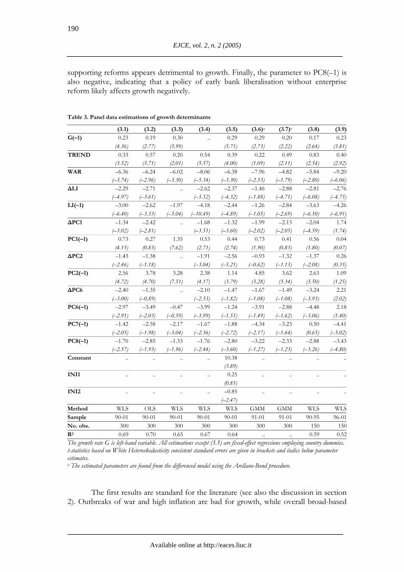

Karsten Staehr Reforms and Economic Growth in Transition Economies
Available online at httpeacesliucit
191
reforms are good for growth The new insights are mainly related to the estimates of the effects of unsynchronised reforms ie the effects of PC2 PC6 PC7 and PC8
52 Robustness
Column (32) in Table 3 presents the estimates obtained using ordinary pooled
least squares (OLS) instead of WLS All signs are retained but the parameter estimate to PC1(ndash1) has fallen and is now insignificant22 The estimated parameters and standard errors to ∆PC6 PC6(ndash1) PC7(ndash1) and PC8(ndash1) have also changed to some extent It seems appropriate whenever possible to use WLS
As discussed above endogeneity problems related to contemporary variables might bias the results We have re-estimated regression (31) without ∆LI ∆PC1 ∆PC2 and ∆PC6 The results reported in (33) show that the parameters to the lagged level of the variables LI(ndash1) PC1(ndash1) PC2(ndash1) PC6(ndash1) PC7(ndash1) and PC8(ndash1) have broadly retained their size and significance In practice the endogeneity problem associated with the variables based on EBRD indices is probably not serious as the indices are scored in the middle of the year when little information about the countryrsquos performance is known
Outliers could influence results unduly particularly the large negative growth rates registered for a number of CIS countries For example output contracted 526 in Armenia in 1992 This partly reflects the war in the country at that time but may also be the result of underreporting We replace the growth rate by the transformation 100G(100ndashG) which dampens the impact of large negative growth rates but has little impact on positive growth rates of ldquonormalrdquo size The findings (not shown) are close to those in column (31) so data points with extreme growth rates do not ldquodriverdquo the results Moreover experiments with transformations of other variables and inclusion of dummies to pick up outliers also show that the results are reasonably robust partly because the equations are estimated using WLS
It is relatively uncommon to include the lagged growth rate on the right-hand side of growth regressions for transition economies23 To ensure that our results do not hinge on this specification G(ndash1) is excluded and the results shown in column (34) The main effect is that the parameter to TREND increases With the exception of the parameter to PC1(ndash1) all other parameters increase somewhat numerically This result is intuitive and the medium-term impacts are broadly the same as before as the dynamic effect from the lagged growth rate is now lacking Removing the trend also has a negligible impact on the results (not shown)
To check the robustness of our results we estimate the growth equation dropping the fixed effect dummies and including instead the two variables capturing initial conditions together with a constant The results in column (35) are close to those in column (31) suggesting that the estimated impact of the reform variables is not a mirage caused by different initial conditions affecting both reform choices and growth results INI2 is significant and has the expected negative sign while INI1 is insignificant
22 The problem of obtaining a precise estimate to PC(ndash1) will reappear in a number of the specifications
used for robustness checks 23 Berg et al (1999) include the lagged growth rate on the right-hand side of the regression but find that it
is insignificant
192
EJCE vol 2 n 2 (2005)
Available online at httpeacesliucit
OLS-based estimation methods can yield biased estimates in dynamic panels due to correlation between the country-specific fixed effects and the error term There is still no consensus on which estimation method to use in this case The often-used Arellano-Bond GMM method first eliminates country-specific effects by differencing the equation and then use lagged values of the level variables as GMM instruments24
However GMM estimation like the Arellano-Bond method gives rise to bias in small samples in particular when right-hand side variables are serially correlated Indeed Judson and Owen (1999) show that in a sample with few cross-sections and a short time horizon the Arellano-Bond method performs no better than the fixed-effect OLS estimator (although better than standard OLS without fixed effects) Other methods are likely to perform better depending on the structure of data Beck and Levine (2004) point out that estimates from the Arellano-Bond method could be strongly biased in small-sample dynamic panels with persistent right-hand side variables Nerlove (2002) argues that the Arellano-Bond method is inappropriate in dynamic panels with a short time dimension and examines the properties of a number of other methods without finding any generally superior estimator 25
As a robustness check we estimate the dynamic model with trend using the Arellano-Bond GMM method In the first case we only instrument the lagged growth rate assuming that the contemporaneous right-hand variables (∆LI ∆PC1 ∆PC2 and ∆PC6) are weakly exogenous The results using the Arellano-Bond one-step method are presented in column (36) Although some changes occur the results in (36) are broadly in line with the results of the WLS estimation in (31) and with the OLS estimation in (33) (Note that the Arellano-Bond procedure implies that the sample is reduced one period)
Column (37) shows the results when the contemporaneous variables (∆LI ∆PC1 ∆PC2 and ∆PC6) are also instrumented using Arelleno-Bond level instruments This should eliminate possible endogeneity biases from the contemporaneous right-hand variables Again the changes are not dramatic
The conclusion is that GMM estimation confirms the qualitative results obtained earlier The estimated standard errors are generally larger for the GMM estimations than for the OLSWLS estimations This problem is to some extent related to the ldquoweak instrument problemrdquo causing the GMM estimators to be inefficient in small samples26 We find as do several other studies that the GMM results are not fundamentally different from least-squares-based methods They may however suffer from inference problems
When the sample is split into two subperiods some instability is revealed The estimation results are shown for 1990-95 in column (310) and for 1996-2001 in column (311) The estimation results for the early subperiod correspond closely to the full sample results with the exception of the estimate to PC7(ndash1) which is positive albeit insignificant For the latter subperiod a number of changes are noteworthy First the 24 Instrumentation is required as the error term of the difference equation is still correlated with the left-
hand side variable 25 This is also reflected in eg Pattillo et al (2002) where dynamic growth models are estimated All results
are presented using four different estimation techniques including GMM 26 The use of the Arellano-Bond method is not rejected There is first-order autocorrelation in the
residuals in the differenced model and the Sargan test does not reject the instruments Nevertheless the presence of serially correlated right-hand variables reduces the efficiency of the level instruments The potential small-sample bias is an argument for avoiding a general-to-specific specification search using GMM
Karsten Staehr Reforms and Economic Growth in Transition Economies
Available online at httpeacesliucit
193
parameters to ∆PC1 and ∆PC2 are now positive although none of the variables are significant at the 5 level The short-term costs of reforms seem at most to be a feature of the early stages of transition Second the estimated parameters to PC1(ndash1) and PC2(ndash1) have dropped substantially However the changes to the parameters to ∆PC1 and ∆PC2 combined with the changes to PC1(ndash1) and PC2(ndash1) imply that the effects of the two reform clusters in the 2-4 years interval are broadly unchanged What has changed is merely the adjustment dynamics Third ∆PC6 and PC6(ndash1) have changed sign while PC7(ndash1) is highly significant in the late period In sum reforms do a better job of explaining growth at the beginning of the reform period than at the end A number of studies reach this conclusion eg Radulescu and Barlow (2002) This is consistent with the view that reforms change the structure of these economies likely increasing the importance of traditional growth factors like physical and human capital accumulation
The estimations reported employ ldquocalendar timerdquo Calendar time ndash as opposed to ldquotransition timerdquo ndash is chosen because it gives the longest possible sample ensures more variation in both right-hand and left-hand variables and simplifies interpretation in certain cases As a robustness check most of the regressions in this paper have been re-estimated using transition time using the correspondence suggested in Berg et al (1999) The results (not shown) are broadly similar to those reported The main difference is that the estimates to ∆PC1 and ∆PC2 although still negative tend not to be significant at conventional levels This result is broadly in line with the above finding that the negative and significant parameters to ∆PC1 and ∆PC2 are derived from the early part of the sample (which is shortened for many countries when transition time is used)27
53 Results and discussion
The broadly similar results obtained from many specifications suggest that
several fairly robust conclusions can be drawn concerning the relationship between reforms and growth in transition countries The control variables offer straightforward interpretations Conflict situations affect growth negatively while the lagged growth rate and a trend always attain positive signs
Inflation and increasing inflation are negatively correlated with growth The contemporaneous effect of inflation changes is negative even in the later half of the sample ie there still appears to be no short-term Phillips curve relationship in the transition economies
We find that broad-based reforms as represented by principal component PC1 are good for growth in the medium term while the short-term effect may be negative at the early stages of reform The parameter to PC1(ndash1) has been estimated to values ranging from 022 to 073 (and 135 in an extremely under-parameterised model) This rather broad interval of estimates is somewhat inconvenient as PC1 captures the overall reform progress and different parameter sizes have different implications for the desirability of reforms28
27 Additional robustness tests can be found in the working paper version of this paper Staehr (2003) 28 The result is however consistent with previous contributions which have found a wide range of
estimated parameter values to a broad index of reforms (see discussion in Radulescu and Barlow 2002) Radulescu and Barlow (2002) use an extreme bounds analysis and show that the sum of the EBRD indices does not enter robustly in their growth regressions ie the parameter and the significance of the
194
EJCE vol 2 n 2 (2005)
Available online at httpeacesliucit
Early reforms in the form of liberalisation and small-scale privatisation have a positive medium-term effect on growth even in the absence of other (mainly structural) reforms Liberalisation and small-scale privatisation have a positive effect on growth even if structural reforms are less advanced The short-term impact of early liberalisation appears to be negative at the early stages of reform
A policy of large-scale privatisation and price liberalisation without small-scale privatisation and market opening has a negative impact on growth The impact is contemporaneous as well as medium-term This result broadly confirms the finding in Zinnes et al (2001) that privatisation without enterprise reforms leads to title change with little restructuring Broadly similar results follow from the meta-analysis in Djankov and Murrell (2002) of approximately 100 empirical studies examining restructuring at the enterprise level Fast privatisation of large firms with insufficient supporting reforms hold back firm restructuring and growth (see also Havrylyshyn 2001) Note however that the result implies rapid small-scale privatisation is beneficial to growth even in the absence of large-scale privatisation and price liberalisation
Early market opening without other reforms like small-scale privatisation and enterprise restructuring also seems detrimental to growth at least in the latter part of transition Figuratively one might imagine foreign competition sweeping away domestic state-owned and unreconstructed producers Crafts (2000) and IMF (1997) discuss preconditions necessary to ensure that market opening and international integration is beneficial to growth Again the reasoning can be reversed a policy of small-scale privatisation and enterprise restructuring appear growth enhancing minus even when not backed by market opening
Finally bank liberalisation without enterprise restructuring has a negative impact on growth especially in the later stages of reform An example of this might be the Czech experience in the mid-1990s when excessive bank lending to non-restructured firms contributed to serious banking sector problems and unsatisfactory growth (see OECD 1998 and 2000) The reverse interpretation is that enterprise restructuring is beneficial even in the absence of bank liberalisation
6 Speed of reforms
The speed at which reforms should be introduced and implemented remains a controversial issue within transition economics The debate also covers sequencing and reform complementary as sequenced reforms may take longer to implement than broad-based reforms This section focuses on the effect on growth of speed per se ie the overall speed with which reforms are implemented29
As noted in section 2 an argument for speedy reform exists when the reform level affects growth positively Fast reforms would put the country on a higher path early on allowing the country to enjoy higher growth for a longer period In this sense all estimations presented in section 5 suggest that broad-based reforms (PC1) or
parameter depend on other variables in the regressions Fidrmuc (2003) also found that it is difficult to estimate the parameter to broad-based reforms precisely
29 The speed of reforms is also important for objectives other than growth eg distribution regional development and medium-term political sustainability These issues cannot be addressed in this framework
Karsten Staehr Reforms and Economic Growth in Transition Economies
Available online at httpeacesliucit
195
liberalisation (PC2) should be implemented rapidly30 However as argued in section 2 we are interested in effects on top of this level effect
Testing directly for speed effects presents two challenges We must specify precise and testable hypotheses and then derive and implement tests of those hypotheses Here we consider two hypotheses First speed effects may affect the level of ldquopainrdquo resulting from reforms in the short term Second the speed of reforms may affect medium-term growth and therefore influence the selection of growth path The short-term hypothesis is examined by testing for possible convexity in the short-term reform costs The medium-term hypothesis is tested by the construction of variables that capture respectively the divergence of the actual reform level from the trend level and indicator variables for a countryrsquos rate of reform
61 Non-linearities in short-term costs
The estimations in section 5 implicitly assumed that short-term reform changes
affect growth rates linearly This assumption implies that the short-term costs of reforms are the same whether reforms are implemented quickly or done piecemeal over several years However possible convexities in the short-term impact would imply ceteris paribus that the level of transition ldquopainrdquo might be lower in a slow reform regime
The search for short-term convexities is narrowed to the first two principal components The starting point for our search for convexities is regression (31) in Table 3 For ease of comparison we repeat this regression in column (41) in Table 4 We test first for possible convexities in the link between ∆PC1 and growth ∆PC1 is replaced by the transformation (137+∆PC1)α where α is the parameter allowing for non-linear effects and 137 is added to ensure that the argument is always positive We perform a grid search by varying α = 01 02 hellip searching for the α-value leading to the parameter estimate with the highest t-value The result is shown in column (42) in Table 4 A similar procedure is performed for ∆PC2 with β varied to give the most precise estimate of (141+∆PC2)β The result appears in column (43)
For the term containing ∆PC1 the t-value was maximised for α = 123 while the t-value for the term containing ∆PC2 was maximised for β = 16 There seems to be a high degree of convexity in the short-term growth costs of broad-based reform and a moderate degree in the liberalisation term
The results are obtained in spite of the test being biased against detecting non-linear effects as only linear variables were used in the specification search Still the test has little power In the specification shown in (42) we have added ∆PC1 as a separate right-hand side variable to ldquocompeterdquo with (137+∆PC1)123
The parameters to both (137+∆PC1)123 and ∆PC1 are negative but insignificant A Wald test cannot reject the joint hypothesis that the parameter to (137+∆PC1)123 is 0 and the parameter to ∆PC1 is ndash229 (as in the original specification) We conclude that although the convex specification yields a slightly more precise parameter estimate the difference is not statistically significant The same holds for the convex specification of ∆PC2
30 Naturally the opposite holds for the unsynchronised reforms of the types captured by PC6 PC7 and
PC8
196
EJCE vol 2 n 2 (2005)
Available online at httpeacesliucit
Table 4 Speed effects in panel data estimations of growth determinants
(41)a (42) (43) (44) (45) (46)
023 026 023 032 027 027G(ndash1)
(436) (498) (436) (553) (549) (568)033 030 033 042 060 070TREND
(352) (342) (352) (271) (541) (643)ndash636 ndash594 ndash642 ndash314 ndash647 ndash633WAR
(ndash374) (ndash387) (ndash381) (ndash155) (ndash330) (ndash319)ndash229 ndash232 ndash222 ndash132 ndash243 ndash243∆LI
(ndash497) (ndash559) (ndash486) (ndash228) (ndash441) (ndash445)ndash300 ndash310 ndash298 ndash219 ndash262 ndash265LI(ndash1)
(ndash640) (ndash741) (ndash642) (ndash324) (ndash518) (ndash536)ndash134 ndash117 ndash001 ndash151 ndash162∆PC1
(ndash302) (ndash254) (ndash002) (ndash420) (ndash502)073 082 073 023 036 039PC1(ndash1)
(415) (496) (412) (053) (232) (276)ndash143 ndash123 142 ndash249 ndash247∆PC2
(ndash246) (ndash206) (193) (ndash511) (ndash551)256 238 246 351 108 080PC2(ndash1)
(472) (488) (450) (454) (350) (260)ndash240 ndash291 ndash241 ndash227 ndash137 ndash142∆PC6
(ndash300) (ndash369) (ndash302 (ndash207) (ndash171) (ndash185)ndash297 ndash312 ndash301 ndash169 ndash128 ndash115PC6(ndash1)
(ndash291) (ndash319) (ndash295) (ndash115) (ndash161) (ndash150)ndash142 ndash121 ndash147 ndash280 ndash187 ndash170PC7(ndash1)
(ndash205) (ndash177) (ndash209) (ndash269) (ndash280) (ndash251)ndash170 ndash116 ndash165 ndash105 ndash217 ndash208PC8(ndash1)
(ndash257) (ndash173) (ndash248) (ndash124) (ndash273) (ndash276) ndash313middot10ndash8 (137 + ∆PC1)123
(ndash436) ndash08 (141 + ∆PC2)16
(ndash262) 012 PC1SP
(062) 1038 1006Constant
(392) (387) 003 INI1
(009) ndash098 INI2
(ndash290) ndash054 YEAR
(ndash414) ndash377FAST
(ndash688) ndash312SLOW
(ndash503)Method WLS WLS WLS WLS WLS WLSSample 90-01 90-01 90-01 93-01 90-01 90-01No observations 300 300 300 225 300 300R2 069 068 069 062 066 066The growth rate G is left-hand variable t-statistics based on White Heteroskedasticity consistent standard errors are given in brackets and italics below parameter estimates a For ease of comparison column (41) repeats column (31) from Table 3
Karsten Staehr Reforms and Economic Growth in Transition Economies
Available online at httpeacesliucit
197
62 Divergence from trend reform path We construct a variable that directly reflects the speed of reforms based on a
suggestion in Berg et al (1999) The idea is to calculate the trend reform level during a fixed time window and then compare the actual reform level with the calculated trend value during the early part of the window The higher the early reform level is above trend level the speedier the implementation of reforms
The implementation speed of broad-based reforms is considered within a four-year window We follow the convention in econometrics and use no time indication of the current realisation of a variable We use τ to indicate years from current year Thus τ = 0 indicates the current year τ = ndash1 indicates a one year lag τ = ndash2 indicates a two year lag etc With this notation the contemporaneous reform level is PC1 and the reform level in year τ ie the reform level lagged τ years is PC1(τ)
We consider a four-year window preceding the current year The total change in the reform index during the four year period is [PC1 ndash PC1(ndash4)] and the average annual change is [PC1 ndash PC1(ndash4)]4 Accordingly the expected trend reform level for any year in the four-year window preceding the current year is
EPC1(τ) = PC1(ndash4) + (4 + τ)middot[PC1 ndash PC1(ndash4)]4 where τ = ndash4 hellip ndash1 For τ = ndash4 EPC1(τ) = PC1(τ) while EPC1(τ) increases
linearly with the annual rate of reform change for τ = ndash3 ndash2 ndash1 The speed variable PC1SP is the sum of the differences between the actual and the trend reform level for years τ = ndash3 and τ = ndash2
PC1SP = [PC1(ndash3) ndash EPC1(ndash3)] + [PC1(ndash2) ndash EPC1(ndash2)] PC1SP is added to specification (31) with the result shown in column (44) in
Table 4 Note that the sample period has changed as PC1SP absorbs three years of the sample The parameter to PC1SP is positive but insignificant31 It should be noted however that the regression contains many variables which could make it difficult for PC1SP to attain significance The partial correlation between G and PC1SP is positive and highly significant Still experiments with different samples non-linear transformations and lagged values of PC1SP show that no stable relationship exists On the suspicion of asymmetric effects we split PC1SP into two variables respectively containing positive and negative values but the results (not shown) were again inconclusive Similar exercises using the liberalisation cluster (PC2) fail to yield any consistent results
63 Scoring of reform speed
Finally we apply methods derived from Wolf (1999) to test for speed effects Initially the number of years from the start of the reform process (ie year 0 using
31 The parameter to ∆PC1 is now insignificant This is the consequence of the shorter sample (also see
(39) in Table 3) and the exclusion of PC1SP
198
EJCE vol 2 n 2 (2005)
Available online at httpeacesliucit
transition time) until PC1 has increased by 4 is counted32 This number (score) would be eg 2 for the Czech Republic and Estonia 4 for Hungary and Moldova and 7 for Bulgaria and Croatia For some countries eg Belarus and Macedonia PC1 does not increase by 4 units within by 2001
The variable YEAR is constructed as follows For 1989-1997 it contains zeros for 1998-2001 it contains the speed score provided the score is less than 8 otherwise zero The construction of YEAR with zeros until 1998 implies that only medium-term effects of the speed score are captured and ensures that the measure of reform speed does not affect growth before reforms are actually implemented33
We include YEAR in regression (35) with a constant term and controls for initial conditions (Fixed effects estimation cannot be used when YEAR is included) The result is shown in column (45) in Table 4 The estimated parameter is negative and significant indicating that reform speed is positively correlated with growth ie rapid reform is associated with higher medium-term growth
Another test separates the transition countries into three groups The first group consists of countries undertaking fast reforms (YEAR le 3) the second group consists of countries undertaking gradual reforms (4 le YEAR le 7) and the third group contains reform-resistant laggards (YEAR ge 8) The dummy FAST has zeros for 1989-97 and ones for 1998-2001 for all countries in the first group The dummy SLOW has zeros for 1989-97 and ones for countries in the second group Column (46) in Table 4 shows the result of adding these two dummy variables to regression (35) Both have negative (and significant) parameters The parameter to FAST is smaller than to SLOW which may indicate that slow reforms were beneficial to growth However the Wald test cannot reject the hypothesis that the two parameters are identical
The method of directly inserting the variables YEAR or FAST and SLOW into the growth regression did not provide firm evidence on the effect of speed However there is no evidence that speedy reforms hampered medium-term growth
64 Discussion
Early reforms allow more years in which the transition country can reap the benefits Beyond this trivial finding the panel data methodology employed in this paper does not provide strong arguments for or against rapid reform The short-term cost of reforms might be larger when implemented in bulk but the effect is small and insignificant The medium-term growth effects of rapid reform are uncertain but rapid reforms appear unlikely to hamper growth In sum the speed of reforms does not appear to a quantitatively substantial impact on growth over and above the level effect This result is in conflict with the conclusions in World Bank (1996) and Berg et al (1999) but is broadly in line with Wolf (1999)
32 For a country starting with all reform indices at their lowest level (eg most countries emerging from
the Soviet Union) an increase of PC1 equal to 4 signifies that the country is halfway to a well-developed market economy
33 It also implies that the variable YEAR only contributes to explaining growth in the last four years of the sample 1990-2001 ie the part of the sample where the other right-hand variables are relative less effective
Karsten Staehr Reforms and Economic Growth in Transition Economies
Available online at httpeacesliucit
199
7 Final comments
A novel feature of this paper was the use of principal component clustering of the EBRD reform indices to infer the structure of reform in transition economies A cluster of synchronised broad-based reforms ie liberalisation privatisation and structural reforms covers 795 of all variation in the initial EBRD reform indices A cluster of liberalisation and small-scale reforms without other reforms explains 79 of the variation while six other clusters of unsynchronised reforms span the remaining 126
The growth regressions included the reform clusters inflation terms and control variables As in most other studies inflation was found to be detrimental to growth Synchronised broad-based reforms had a positive impact on growth in the medium term with a negative short-term effect at the early stages of reform Also a policy of liberalisation and small-scale privatisation without accompanying structural reforms were shown to have a positive effect (again with a possible early negative short-term effect) Accelerated large-scale privatisation without small-scale privatisation and structural reforms were found likely to harm growth both in the short and the medium term
Conversely small-scale privatisation without large-scale privatisation appears beneficial to growth A less certain result is that market opening and price liberalisation without accompanying privatisation and enterprise reforms appear correlated with lower growth but this effect stems primarily for the most recent period Reversing this result privatisation and restructuring without market opening may be good for growth Finally bank liberalisation without enterprise restructuring might be harmful while enterprise reforms without bank liberalisation may increase growth
Effects from the speed of reforms are mostly absent with the exception that early reforms leave the transition country a longer period in which to reap the benefits of reforms Possible negative short-term effects of rapid reforms are likely to be modest and could be balanced by possible positive medium-term effects The broad overall conclusion is that speed per se has no discernible impact on growth
Finally what can we now say about the three questions raised in the introduction
First the analysis revealed a complex pattern of reform complementarities with notable implications for the sequencing of reforms Balanced wide-ranging reforms based on simultaneous progress in liberalisation privatisation and structural reforms are favourable to growth and hence suggest a mutually reinforcing effect of various reform elements
Liberalisation combined with small-scale privatisation is beneficial even in the absence of other reforms In this case unsynchronised reforms produce positive growth effects Thus liberalisation and small-scale privatisation are not perfectly complementary to deeper reforms such as large-scale privatisation and structural reforms A sequenced reform policy that stresses liberalisation and small-scale privatisation is beneficial Early ldquoeasyrdquo reforms should therefore not be postponed in the absence of a comprehensive reform strategy
A number of unsynchronised reform packages proved detrimental to growth Sequenced policy packages involving large-scale privatisation without small-scale privatisation market opening without accompanying reforms and bank liberalisation without enterprise restructuring lead to lower growth in the short andor medium term Conversely a ldquoreversalrdquo of the policy mix would produce packages beneficial to growth
200
EJCE vol 2 n 2 (2005)
Available online at httpeacesliucit
In sum the statistically significant parameters to a number of unsynchronised reform clusters support the view that reforms need to be fine-tuned to take into account complex interactions among reforms
Second we asked which reforms are of foremost importance Within the set of variables used in this paper and using a broad brush a number of variables stand out Inflation stabilisation repeatedly proved important Price liberalisation small-scale privatisation enterprise restructuring (and to a lesser degree trade opening) were generally important in many different combinations with other reforms Large-scale privatisation financial sector reforms and market regulation mainly proved beneficial when they were part of a larger more comprehensive reform packages These results seem to support the view that reform policies are crucial minus even countries that fail to attempt deep structural changes can gain from reforms These findings are broadly in line with the findings in Havrylyshyn and van Rooden (2000) As a caveat we note that only a few variables included in our analysis reflect currently popular themes such as institutional quality and social capital
Third the finding that speed per se is of little importance for growth seems to favour relatively rapid implementation of reforms due to the level effect However this finding also implies there is no direct loss from slowing reforms when it is necessary to get content or sequencing right
These results probably disappoint supporters of big-bang as well as supporters of gradualism as they provide no unequivocal support for either view If it is any consolation to the gradualists reform sequencing appears to be important and reforms should preferably progress synchronously Certain sequenced reform paths are clearly counterproductive Likewise for the big-bang supporters initial phase reforms are beneficial even in the absence of deeper reforms Moreover fast reforms appear generally beneficial Thus there is no clear-cut transition strategy that provides the best results for countries endeavouring to convert a centrally planned economy into a market economy There are only policy choices minus some better than others minus and certain strategies that should be avoided
References
Ahrens J Meurers M (2002) lsquoHow Governance Affects the Quality of Policy Reform and Economic Performance New Evidence for Economies in Transitionrsquo Journal for Institutional Innovation Development and Transition 6 35-56
Aslund A (2002) Building Capitalism The Transformation of the Former Soviet Bloc Cambridge University Press Cambridge
Aziz J Wescott R (1997) lsquoPolicy Complementarities and the Washington Consensusrsquo IMF Working Paper No118
Beck T Levine R (2004) lsquoStock Markets Banks and Growth Panel Evidencersquo Journal of Banking and Finance 28 423-442
Berg A Borensztein E Sahay R Zettelmeyer J (1999) lsquoThe Evolution of Output in the Transition Economies Explaining the Differencesrsquo IMF Working Paper No73
Blanchard O Dornbusch R Krugman P Layard R Summers L (1991) Reform in Eastern Europe MIT Press Cambridge MA
Campos N Coricelli F (2002) lsquoGrowth in Transition What We Know What We Donrsquot and What We Shouldrsquo Journal of Economic Literature 90 793-836
Karsten Staehr Reforms and Economic Growth in Transition Economies
Available online at httpeacesliucit
201
Correa R (2002) lsquoThe Washington Consensus in Latin America A Quantitative Evaluationrsquo mimeo San Francisco de Quito University Ecuador
Crafts N (2000) lsquoGlobalization and Growth in the Twentieth Centuryrsquo in Prasad E (ed) Supporting Studies for the World Economic Outlook International Monetary Fund Washington DC
de Melo M Denizer C Gelb A (1997) lsquoFrom Plan to Market Patterns of Transitionrsquo in Blejer M Skreb M (eds) Macroeconomic Stabilization in Transition Economies Cambridge University Press Cambridge
de Melo M Denizer C Gelb A (2001) lsquoCircumstance and Choice The Role of Initial Conditions and Policies in Transition Economiesrsquo World Bank Economic Review 15 1-31
Djankov S Murrell P (2002) lsquoEnterprise Restructuring in Transition A Quantitative Surveyrsquo Journal of Economic Literature 90 739-792
EBRD (1999-2004) Transition Report European Bank for Reconstruction and Development Fidrmuc J (2003) lsquoEconomic Reform Democracy and Growth during Post Communist
Transitionrsquo European Journal of Political Economy 19 583-604 Fischer S Gelb A (1991) lsquoThe Process of Socialist Economic Transformationrsquo Journal of
Economic Perspectives 5 91-105 Fischer S Sahay R (2000) lsquoThe Transition Economies After Ten Yearsrsquo IMF Working Paper
No30 Fischer S Sahay R Vegh C (1996a) lsquoStabilization and Growth in Transition Economies The
Early Experiencersquo Journal of Economic Perspectives 10 45-66 Fischer S Sahay R Vegh C (1996b) lsquoEconomies in Transition The Beginnings of Growthrsquo
American Economic Review 86 229-233 Havrylyshyn O van Rooden R (2000) lsquoInstitutions Matter in Transition but so do Policiesrsquo
IMF Working Paper No70 Havrylyshyn O (2001) lsquoRecovery and Growth in Transition A Decade of Evidencersquo IMF Staff
Paper 48 53-87 Havrylyshyn O Izvorski I van Rooden R (1998) lsquoRecovery and Growth in Transition
Economies 1990-97 A Stylized Regression Analysisrsquo IMF Working Paper No141 Heybey B Murrell P (1999) lsquoThe Relationship Between Economic Growth and the Speed of
Liberalization During the Transitionrsquo Policy Reform 3 121-37 IMF (1997) World Economic Outlook Globalization Opportunities and Challenges May chapter IV IMF (2000) World Economic Outlook Focus on Transition Economies October chapter III Judson R Owen A (1999) lsquoEstimating Dynamic Panel Data Models A Practical Guide for
Macroeconomistsrsquo Economics Letters 65 9-15 Nerlove M (2002) lsquoProperties of Alternative Estimators of Dynamic Panel Models An
Empirical Analysis of Cross-Country Data for the Study of Economic Growthrsquo in Nerlove M Essays in Panel Data Econometrics Cambridge University Press Cambridge
Nsouli S Rached M Funke N (2002) lsquoThe Speed of Adjustment and the Sequencing of Economic Reforms Issues and Guidelines for Policymakersrsquo IMF Working Paper No132
OECD (1998) OECD Economic Surveys Czech Republic May OECD OECD (2000) OECD Economic Surveys Czech Republic February OECD Pattillo C Poirson H Ricca L (2002) lsquoExternal Debt and Growthrsquo IMF Working Paper No69 Radulescu R Barlow D (2002) lsquoThe Relation between Policies and Growth in Transition
Countriesrsquo Economics of Transition 10 719-745 Roland G (2001) lsquoTen Years After hellip Transition and Economicsrsquo IMF Staff Papers 48 29-52
202
EJCE vol 2 n 2 (2005)
Available online at httpeacesliucit
Sachs J Zinnes G Eilat Y (2000) lsquoPatterns of Economic Reform and its Determinants in Transition Economies 1990-1998rsquo Harvard Institute for International Development CAER II Discussion Paper No 61
Staehr K (2003) lsquoReforms and Economic Growth in Transition Economies Complementarity Sequencing and Speedrsquo BOFIT Discussion Paper No1
Stiglitz J (2001) lsquoWhither Reform Ten Years of Transitionrsquo in Pleskovic B Stiglitz J (eds) World Bank Annual Bank Conference on Development Economics 1999 World Bank Washington DC
Wacziarg R (2002) lsquoReview of Easterlyrsquos The Elusive Quest for Growthrsquo Journal of Economic Literature 90 907-918
Wolf H (1999) lsquoTransition Strategies Choices and Outcomesrsquo Princeton Studies in International Finance No85
World Bank (1996) World Development Report 1996 From Plan to Market World Bank Washington DC
World Bank (2002) Transition The First Ten Years Analysis and Lessons for Eastern Europe and the former Soviet Union World Bank Washington DC
Zinnes C Eilat Y Sachs J (2001) lsquoThe Gains from Privatization in Transition Economies Is lsquoChange of Ownershiprsquo Enoughrsquo IMF Staff Papers 48 146-169

Karsten Staehr Reforms and Economic Growth in Transition Economies
Available online at httpeacesliucit
193
parameters to ∆PC1 and ∆PC2 are now positive although none of the variables are significant at the 5 level The short-term costs of reforms seem at most to be a feature of the early stages of transition Second the estimated parameters to PC1(ndash1) and PC2(ndash1) have dropped substantially However the changes to the parameters to ∆PC1 and ∆PC2 combined with the changes to PC1(ndash1) and PC2(ndash1) imply that the effects of the two reform clusters in the 2-4 years interval are broadly unchanged What has changed is merely the adjustment dynamics Third ∆PC6 and PC6(ndash1) have changed sign while PC7(ndash1) is highly significant in the late period In sum reforms do a better job of explaining growth at the beginning of the reform period than at the end A number of studies reach this conclusion eg Radulescu and Barlow (2002) This is consistent with the view that reforms change the structure of these economies likely increasing the importance of traditional growth factors like physical and human capital accumulation
The estimations reported employ ldquocalendar timerdquo Calendar time ndash as opposed to ldquotransition timerdquo ndash is chosen because it gives the longest possible sample ensures more variation in both right-hand and left-hand variables and simplifies interpretation in certain cases As a robustness check most of the regressions in this paper have been re-estimated using transition time using the correspondence suggested in Berg et al (1999) The results (not shown) are broadly similar to those reported The main difference is that the estimates to ∆PC1 and ∆PC2 although still negative tend not to be significant at conventional levels This result is broadly in line with the above finding that the negative and significant parameters to ∆PC1 and ∆PC2 are derived from the early part of the sample (which is shortened for many countries when transition time is used)27
53 Results and discussion
The broadly similar results obtained from many specifications suggest that
several fairly robust conclusions can be drawn concerning the relationship between reforms and growth in transition countries The control variables offer straightforward interpretations Conflict situations affect growth negatively while the lagged growth rate and a trend always attain positive signs
Inflation and increasing inflation are negatively correlated with growth The contemporaneous effect of inflation changes is negative even in the later half of the sample ie there still appears to be no short-term Phillips curve relationship in the transition economies
We find that broad-based reforms as represented by principal component PC1 are good for growth in the medium term while the short-term effect may be negative at the early stages of reform The parameter to PC1(ndash1) has been estimated to values ranging from 022 to 073 (and 135 in an extremely under-parameterised model) This rather broad interval of estimates is somewhat inconvenient as PC1 captures the overall reform progress and different parameter sizes have different implications for the desirability of reforms28
27 Additional robustness tests can be found in the working paper version of this paper Staehr (2003) 28 The result is however consistent with previous contributions which have found a wide range of
estimated parameter values to a broad index of reforms (see discussion in Radulescu and Barlow 2002) Radulescu and Barlow (2002) use an extreme bounds analysis and show that the sum of the EBRD indices does not enter robustly in their growth regressions ie the parameter and the significance of the
194
EJCE vol 2 n 2 (2005)
Available online at httpeacesliucit
Early reforms in the form of liberalisation and small-scale privatisation have a positive medium-term effect on growth even in the absence of other (mainly structural) reforms Liberalisation and small-scale privatisation have a positive effect on growth even if structural reforms are less advanced The short-term impact of early liberalisation appears to be negative at the early stages of reform
A policy of large-scale privatisation and price liberalisation without small-scale privatisation and market opening has a negative impact on growth The impact is contemporaneous as well as medium-term This result broadly confirms the finding in Zinnes et al (2001) that privatisation without enterprise reforms leads to title change with little restructuring Broadly similar results follow from the meta-analysis in Djankov and Murrell (2002) of approximately 100 empirical studies examining restructuring at the enterprise level Fast privatisation of large firms with insufficient supporting reforms hold back firm restructuring and growth (see also Havrylyshyn 2001) Note however that the result implies rapid small-scale privatisation is beneficial to growth even in the absence of large-scale privatisation and price liberalisation
Early market opening without other reforms like small-scale privatisation and enterprise restructuring also seems detrimental to growth at least in the latter part of transition Figuratively one might imagine foreign competition sweeping away domestic state-owned and unreconstructed producers Crafts (2000) and IMF (1997) discuss preconditions necessary to ensure that market opening and international integration is beneficial to growth Again the reasoning can be reversed a policy of small-scale privatisation and enterprise restructuring appear growth enhancing minus even when not backed by market opening
Finally bank liberalisation without enterprise restructuring has a negative impact on growth especially in the later stages of reform An example of this might be the Czech experience in the mid-1990s when excessive bank lending to non-restructured firms contributed to serious banking sector problems and unsatisfactory growth (see OECD 1998 and 2000) The reverse interpretation is that enterprise restructuring is beneficial even in the absence of bank liberalisation
6 Speed of reforms
The speed at which reforms should be introduced and implemented remains a controversial issue within transition economics The debate also covers sequencing and reform complementary as sequenced reforms may take longer to implement than broad-based reforms This section focuses on the effect on growth of speed per se ie the overall speed with which reforms are implemented29
As noted in section 2 an argument for speedy reform exists when the reform level affects growth positively Fast reforms would put the country on a higher path early on allowing the country to enjoy higher growth for a longer period In this sense all estimations presented in section 5 suggest that broad-based reforms (PC1) or
parameter depend on other variables in the regressions Fidrmuc (2003) also found that it is difficult to estimate the parameter to broad-based reforms precisely
29 The speed of reforms is also important for objectives other than growth eg distribution regional development and medium-term political sustainability These issues cannot be addressed in this framework
Karsten Staehr Reforms and Economic Growth in Transition Economies
Available online at httpeacesliucit
195
liberalisation (PC2) should be implemented rapidly30 However as argued in section 2 we are interested in effects on top of this level effect
Testing directly for speed effects presents two challenges We must specify precise and testable hypotheses and then derive and implement tests of those hypotheses Here we consider two hypotheses First speed effects may affect the level of ldquopainrdquo resulting from reforms in the short term Second the speed of reforms may affect medium-term growth and therefore influence the selection of growth path The short-term hypothesis is examined by testing for possible convexity in the short-term reform costs The medium-term hypothesis is tested by the construction of variables that capture respectively the divergence of the actual reform level from the trend level and indicator variables for a countryrsquos rate of reform
61 Non-linearities in short-term costs
The estimations in section 5 implicitly assumed that short-term reform changes
affect growth rates linearly This assumption implies that the short-term costs of reforms are the same whether reforms are implemented quickly or done piecemeal over several years However possible convexities in the short-term impact would imply ceteris paribus that the level of transition ldquopainrdquo might be lower in a slow reform regime
The search for short-term convexities is narrowed to the first two principal components The starting point for our search for convexities is regression (31) in Table 3 For ease of comparison we repeat this regression in column (41) in Table 4 We test first for possible convexities in the link between ∆PC1 and growth ∆PC1 is replaced by the transformation (137+∆PC1)α where α is the parameter allowing for non-linear effects and 137 is added to ensure that the argument is always positive We perform a grid search by varying α = 01 02 hellip searching for the α-value leading to the parameter estimate with the highest t-value The result is shown in column (42) in Table 4 A similar procedure is performed for ∆PC2 with β varied to give the most precise estimate of (141+∆PC2)β The result appears in column (43)
For the term containing ∆PC1 the t-value was maximised for α = 123 while the t-value for the term containing ∆PC2 was maximised for β = 16 There seems to be a high degree of convexity in the short-term growth costs of broad-based reform and a moderate degree in the liberalisation term
The results are obtained in spite of the test being biased against detecting non-linear effects as only linear variables were used in the specification search Still the test has little power In the specification shown in (42) we have added ∆PC1 as a separate right-hand side variable to ldquocompeterdquo with (137+∆PC1)123
The parameters to both (137+∆PC1)123 and ∆PC1 are negative but insignificant A Wald test cannot reject the joint hypothesis that the parameter to (137+∆PC1)123 is 0 and the parameter to ∆PC1 is ndash229 (as in the original specification) We conclude that although the convex specification yields a slightly more precise parameter estimate the difference is not statistically significant The same holds for the convex specification of ∆PC2
30 Naturally the opposite holds for the unsynchronised reforms of the types captured by PC6 PC7 and
PC8
196
EJCE vol 2 n 2 (2005)
Available online at httpeacesliucit
Table 4 Speed effects in panel data estimations of growth determinants
(41)a (42) (43) (44) (45) (46)
023 026 023 032 027 027G(ndash1)
(436) (498) (436) (553) (549) (568)033 030 033 042 060 070TREND
(352) (342) (352) (271) (541) (643)ndash636 ndash594 ndash642 ndash314 ndash647 ndash633WAR
(ndash374) (ndash387) (ndash381) (ndash155) (ndash330) (ndash319)ndash229 ndash232 ndash222 ndash132 ndash243 ndash243∆LI
(ndash497) (ndash559) (ndash486) (ndash228) (ndash441) (ndash445)ndash300 ndash310 ndash298 ndash219 ndash262 ndash265LI(ndash1)
(ndash640) (ndash741) (ndash642) (ndash324) (ndash518) (ndash536)ndash134 ndash117 ndash001 ndash151 ndash162∆PC1
(ndash302) (ndash254) (ndash002) (ndash420) (ndash502)073 082 073 023 036 039PC1(ndash1)
(415) (496) (412) (053) (232) (276)ndash143 ndash123 142 ndash249 ndash247∆PC2
(ndash246) (ndash206) (193) (ndash511) (ndash551)256 238 246 351 108 080PC2(ndash1)
(472) (488) (450) (454) (350) (260)ndash240 ndash291 ndash241 ndash227 ndash137 ndash142∆PC6
(ndash300) (ndash369) (ndash302 (ndash207) (ndash171) (ndash185)ndash297 ndash312 ndash301 ndash169 ndash128 ndash115PC6(ndash1)
(ndash291) (ndash319) (ndash295) (ndash115) (ndash161) (ndash150)ndash142 ndash121 ndash147 ndash280 ndash187 ndash170PC7(ndash1)
(ndash205) (ndash177) (ndash209) (ndash269) (ndash280) (ndash251)ndash170 ndash116 ndash165 ndash105 ndash217 ndash208PC8(ndash1)
(ndash257) (ndash173) (ndash248) (ndash124) (ndash273) (ndash276) ndash313middot10ndash8 (137 + ∆PC1)123
(ndash436) ndash08 (141 + ∆PC2)16
(ndash262) 012 PC1SP
(062) 1038 1006Constant
(392) (387) 003 INI1
(009) ndash098 INI2
(ndash290) ndash054 YEAR
(ndash414) ndash377FAST
(ndash688) ndash312SLOW
(ndash503)Method WLS WLS WLS WLS WLS WLSSample 90-01 90-01 90-01 93-01 90-01 90-01No observations 300 300 300 225 300 300R2 069 068 069 062 066 066The growth rate G is left-hand variable t-statistics based on White Heteroskedasticity consistent standard errors are given in brackets and italics below parameter estimates a For ease of comparison column (41) repeats column (31) from Table 3
Karsten Staehr Reforms and Economic Growth in Transition Economies
Available online at httpeacesliucit
197
62 Divergence from trend reform path We construct a variable that directly reflects the speed of reforms based on a
suggestion in Berg et al (1999) The idea is to calculate the trend reform level during a fixed time window and then compare the actual reform level with the calculated trend value during the early part of the window The higher the early reform level is above trend level the speedier the implementation of reforms
The implementation speed of broad-based reforms is considered within a four-year window We follow the convention in econometrics and use no time indication of the current realisation of a variable We use τ to indicate years from current year Thus τ = 0 indicates the current year τ = ndash1 indicates a one year lag τ = ndash2 indicates a two year lag etc With this notation the contemporaneous reform level is PC1 and the reform level in year τ ie the reform level lagged τ years is PC1(τ)
We consider a four-year window preceding the current year The total change in the reform index during the four year period is [PC1 ndash PC1(ndash4)] and the average annual change is [PC1 ndash PC1(ndash4)]4 Accordingly the expected trend reform level for any year in the four-year window preceding the current year is
EPC1(τ) = PC1(ndash4) + (4 + τ)middot[PC1 ndash PC1(ndash4)]4 where τ = ndash4 hellip ndash1 For τ = ndash4 EPC1(τ) = PC1(τ) while EPC1(τ) increases
linearly with the annual rate of reform change for τ = ndash3 ndash2 ndash1 The speed variable PC1SP is the sum of the differences between the actual and the trend reform level for years τ = ndash3 and τ = ndash2
PC1SP = [PC1(ndash3) ndash EPC1(ndash3)] + [PC1(ndash2) ndash EPC1(ndash2)] PC1SP is added to specification (31) with the result shown in column (44) in
Table 4 Note that the sample period has changed as PC1SP absorbs three years of the sample The parameter to PC1SP is positive but insignificant31 It should be noted however that the regression contains many variables which could make it difficult for PC1SP to attain significance The partial correlation between G and PC1SP is positive and highly significant Still experiments with different samples non-linear transformations and lagged values of PC1SP show that no stable relationship exists On the suspicion of asymmetric effects we split PC1SP into two variables respectively containing positive and negative values but the results (not shown) were again inconclusive Similar exercises using the liberalisation cluster (PC2) fail to yield any consistent results
63 Scoring of reform speed
Finally we apply methods derived from Wolf (1999) to test for speed effects Initially the number of years from the start of the reform process (ie year 0 using
31 The parameter to ∆PC1 is now insignificant This is the consequence of the shorter sample (also see
(39) in Table 3) and the exclusion of PC1SP
198
EJCE vol 2 n 2 (2005)
Available online at httpeacesliucit
transition time) until PC1 has increased by 4 is counted32 This number (score) would be eg 2 for the Czech Republic and Estonia 4 for Hungary and Moldova and 7 for Bulgaria and Croatia For some countries eg Belarus and Macedonia PC1 does not increase by 4 units within by 2001
The variable YEAR is constructed as follows For 1989-1997 it contains zeros for 1998-2001 it contains the speed score provided the score is less than 8 otherwise zero The construction of YEAR with zeros until 1998 implies that only medium-term effects of the speed score are captured and ensures that the measure of reform speed does not affect growth before reforms are actually implemented33
We include YEAR in regression (35) with a constant term and controls for initial conditions (Fixed effects estimation cannot be used when YEAR is included) The result is shown in column (45) in Table 4 The estimated parameter is negative and significant indicating that reform speed is positively correlated with growth ie rapid reform is associated with higher medium-term growth
Another test separates the transition countries into three groups The first group consists of countries undertaking fast reforms (YEAR le 3) the second group consists of countries undertaking gradual reforms (4 le YEAR le 7) and the third group contains reform-resistant laggards (YEAR ge 8) The dummy FAST has zeros for 1989-97 and ones for 1998-2001 for all countries in the first group The dummy SLOW has zeros for 1989-97 and ones for countries in the second group Column (46) in Table 4 shows the result of adding these two dummy variables to regression (35) Both have negative (and significant) parameters The parameter to FAST is smaller than to SLOW which may indicate that slow reforms were beneficial to growth However the Wald test cannot reject the hypothesis that the two parameters are identical
The method of directly inserting the variables YEAR or FAST and SLOW into the growth regression did not provide firm evidence on the effect of speed However there is no evidence that speedy reforms hampered medium-term growth
64 Discussion
Early reforms allow more years in which the transition country can reap the benefits Beyond this trivial finding the panel data methodology employed in this paper does not provide strong arguments for or against rapid reform The short-term cost of reforms might be larger when implemented in bulk but the effect is small and insignificant The medium-term growth effects of rapid reform are uncertain but rapid reforms appear unlikely to hamper growth In sum the speed of reforms does not appear to a quantitatively substantial impact on growth over and above the level effect This result is in conflict with the conclusions in World Bank (1996) and Berg et al (1999) but is broadly in line with Wolf (1999)
32 For a country starting with all reform indices at their lowest level (eg most countries emerging from
the Soviet Union) an increase of PC1 equal to 4 signifies that the country is halfway to a well-developed market economy
33 It also implies that the variable YEAR only contributes to explaining growth in the last four years of the sample 1990-2001 ie the part of the sample where the other right-hand variables are relative less effective
Karsten Staehr Reforms and Economic Growth in Transition Economies
Available online at httpeacesliucit
199
7 Final comments
A novel feature of this paper was the use of principal component clustering of the EBRD reform indices to infer the structure of reform in transition economies A cluster of synchronised broad-based reforms ie liberalisation privatisation and structural reforms covers 795 of all variation in the initial EBRD reform indices A cluster of liberalisation and small-scale reforms without other reforms explains 79 of the variation while six other clusters of unsynchronised reforms span the remaining 126
The growth regressions included the reform clusters inflation terms and control variables As in most other studies inflation was found to be detrimental to growth Synchronised broad-based reforms had a positive impact on growth in the medium term with a negative short-term effect at the early stages of reform Also a policy of liberalisation and small-scale privatisation without accompanying structural reforms were shown to have a positive effect (again with a possible early negative short-term effect) Accelerated large-scale privatisation without small-scale privatisation and structural reforms were found likely to harm growth both in the short and the medium term
Conversely small-scale privatisation without large-scale privatisation appears beneficial to growth A less certain result is that market opening and price liberalisation without accompanying privatisation and enterprise reforms appear correlated with lower growth but this effect stems primarily for the most recent period Reversing this result privatisation and restructuring without market opening may be good for growth Finally bank liberalisation without enterprise restructuring might be harmful while enterprise reforms without bank liberalisation may increase growth
Effects from the speed of reforms are mostly absent with the exception that early reforms leave the transition country a longer period in which to reap the benefits of reforms Possible negative short-term effects of rapid reforms are likely to be modest and could be balanced by possible positive medium-term effects The broad overall conclusion is that speed per se has no discernible impact on growth
Finally what can we now say about the three questions raised in the introduction
First the analysis revealed a complex pattern of reform complementarities with notable implications for the sequencing of reforms Balanced wide-ranging reforms based on simultaneous progress in liberalisation privatisation and structural reforms are favourable to growth and hence suggest a mutually reinforcing effect of various reform elements
Liberalisation combined with small-scale privatisation is beneficial even in the absence of other reforms In this case unsynchronised reforms produce positive growth effects Thus liberalisation and small-scale privatisation are not perfectly complementary to deeper reforms such as large-scale privatisation and structural reforms A sequenced reform policy that stresses liberalisation and small-scale privatisation is beneficial Early ldquoeasyrdquo reforms should therefore not be postponed in the absence of a comprehensive reform strategy
A number of unsynchronised reform packages proved detrimental to growth Sequenced policy packages involving large-scale privatisation without small-scale privatisation market opening without accompanying reforms and bank liberalisation without enterprise restructuring lead to lower growth in the short andor medium term Conversely a ldquoreversalrdquo of the policy mix would produce packages beneficial to growth
200
EJCE vol 2 n 2 (2005)
Available online at httpeacesliucit
In sum the statistically significant parameters to a number of unsynchronised reform clusters support the view that reforms need to be fine-tuned to take into account complex interactions among reforms
Second we asked which reforms are of foremost importance Within the set of variables used in this paper and using a broad brush a number of variables stand out Inflation stabilisation repeatedly proved important Price liberalisation small-scale privatisation enterprise restructuring (and to a lesser degree trade opening) were generally important in many different combinations with other reforms Large-scale privatisation financial sector reforms and market regulation mainly proved beneficial when they were part of a larger more comprehensive reform packages These results seem to support the view that reform policies are crucial minus even countries that fail to attempt deep structural changes can gain from reforms These findings are broadly in line with the findings in Havrylyshyn and van Rooden (2000) As a caveat we note that only a few variables included in our analysis reflect currently popular themes such as institutional quality and social capital
Third the finding that speed per se is of little importance for growth seems to favour relatively rapid implementation of reforms due to the level effect However this finding also implies there is no direct loss from slowing reforms when it is necessary to get content or sequencing right
These results probably disappoint supporters of big-bang as well as supporters of gradualism as they provide no unequivocal support for either view If it is any consolation to the gradualists reform sequencing appears to be important and reforms should preferably progress synchronously Certain sequenced reform paths are clearly counterproductive Likewise for the big-bang supporters initial phase reforms are beneficial even in the absence of deeper reforms Moreover fast reforms appear generally beneficial Thus there is no clear-cut transition strategy that provides the best results for countries endeavouring to convert a centrally planned economy into a market economy There are only policy choices minus some better than others minus and certain strategies that should be avoided
References
Ahrens J Meurers M (2002) lsquoHow Governance Affects the Quality of Policy Reform and Economic Performance New Evidence for Economies in Transitionrsquo Journal for Institutional Innovation Development and Transition 6 35-56
Aslund A (2002) Building Capitalism The Transformation of the Former Soviet Bloc Cambridge University Press Cambridge
Aziz J Wescott R (1997) lsquoPolicy Complementarities and the Washington Consensusrsquo IMF Working Paper No118
Beck T Levine R (2004) lsquoStock Markets Banks and Growth Panel Evidencersquo Journal of Banking and Finance 28 423-442
Berg A Borensztein E Sahay R Zettelmeyer J (1999) lsquoThe Evolution of Output in the Transition Economies Explaining the Differencesrsquo IMF Working Paper No73
Blanchard O Dornbusch R Krugman P Layard R Summers L (1991) Reform in Eastern Europe MIT Press Cambridge MA
Campos N Coricelli F (2002) lsquoGrowth in Transition What We Know What We Donrsquot and What We Shouldrsquo Journal of Economic Literature 90 793-836
Karsten Staehr Reforms and Economic Growth in Transition Economies
Available online at httpeacesliucit
201
Correa R (2002) lsquoThe Washington Consensus in Latin America A Quantitative Evaluationrsquo mimeo San Francisco de Quito University Ecuador
Crafts N (2000) lsquoGlobalization and Growth in the Twentieth Centuryrsquo in Prasad E (ed) Supporting Studies for the World Economic Outlook International Monetary Fund Washington DC
de Melo M Denizer C Gelb A (1997) lsquoFrom Plan to Market Patterns of Transitionrsquo in Blejer M Skreb M (eds) Macroeconomic Stabilization in Transition Economies Cambridge University Press Cambridge
de Melo M Denizer C Gelb A (2001) lsquoCircumstance and Choice The Role of Initial Conditions and Policies in Transition Economiesrsquo World Bank Economic Review 15 1-31
Djankov S Murrell P (2002) lsquoEnterprise Restructuring in Transition A Quantitative Surveyrsquo Journal of Economic Literature 90 739-792
EBRD (1999-2004) Transition Report European Bank for Reconstruction and Development Fidrmuc J (2003) lsquoEconomic Reform Democracy and Growth during Post Communist
Transitionrsquo European Journal of Political Economy 19 583-604 Fischer S Gelb A (1991) lsquoThe Process of Socialist Economic Transformationrsquo Journal of
Economic Perspectives 5 91-105 Fischer S Sahay R (2000) lsquoThe Transition Economies After Ten Yearsrsquo IMF Working Paper
No30 Fischer S Sahay R Vegh C (1996a) lsquoStabilization and Growth in Transition Economies The
Early Experiencersquo Journal of Economic Perspectives 10 45-66 Fischer S Sahay R Vegh C (1996b) lsquoEconomies in Transition The Beginnings of Growthrsquo
American Economic Review 86 229-233 Havrylyshyn O van Rooden R (2000) lsquoInstitutions Matter in Transition but so do Policiesrsquo
IMF Working Paper No70 Havrylyshyn O (2001) lsquoRecovery and Growth in Transition A Decade of Evidencersquo IMF Staff
Paper 48 53-87 Havrylyshyn O Izvorski I van Rooden R (1998) lsquoRecovery and Growth in Transition
Economies 1990-97 A Stylized Regression Analysisrsquo IMF Working Paper No141 Heybey B Murrell P (1999) lsquoThe Relationship Between Economic Growth and the Speed of
Liberalization During the Transitionrsquo Policy Reform 3 121-37 IMF (1997) World Economic Outlook Globalization Opportunities and Challenges May chapter IV IMF (2000) World Economic Outlook Focus on Transition Economies October chapter III Judson R Owen A (1999) lsquoEstimating Dynamic Panel Data Models A Practical Guide for
Macroeconomistsrsquo Economics Letters 65 9-15 Nerlove M (2002) lsquoProperties of Alternative Estimators of Dynamic Panel Models An
Empirical Analysis of Cross-Country Data for the Study of Economic Growthrsquo in Nerlove M Essays in Panel Data Econometrics Cambridge University Press Cambridge
Nsouli S Rached M Funke N (2002) lsquoThe Speed of Adjustment and the Sequencing of Economic Reforms Issues and Guidelines for Policymakersrsquo IMF Working Paper No132
OECD (1998) OECD Economic Surveys Czech Republic May OECD OECD (2000) OECD Economic Surveys Czech Republic February OECD Pattillo C Poirson H Ricca L (2002) lsquoExternal Debt and Growthrsquo IMF Working Paper No69 Radulescu R Barlow D (2002) lsquoThe Relation between Policies and Growth in Transition
Countriesrsquo Economics of Transition 10 719-745 Roland G (2001) lsquoTen Years After hellip Transition and Economicsrsquo IMF Staff Papers 48 29-52
202
EJCE vol 2 n 2 (2005)
Available online at httpeacesliucit
Sachs J Zinnes G Eilat Y (2000) lsquoPatterns of Economic Reform and its Determinants in Transition Economies 1990-1998rsquo Harvard Institute for International Development CAER II Discussion Paper No 61
Staehr K (2003) lsquoReforms and Economic Growth in Transition Economies Complementarity Sequencing and Speedrsquo BOFIT Discussion Paper No1
Stiglitz J (2001) lsquoWhither Reform Ten Years of Transitionrsquo in Pleskovic B Stiglitz J (eds) World Bank Annual Bank Conference on Development Economics 1999 World Bank Washington DC
Wacziarg R (2002) lsquoReview of Easterlyrsquos The Elusive Quest for Growthrsquo Journal of Economic Literature 90 907-918
Wolf H (1999) lsquoTransition Strategies Choices and Outcomesrsquo Princeton Studies in International Finance No85
World Bank (1996) World Development Report 1996 From Plan to Market World Bank Washington DC
World Bank (2002) Transition The First Ten Years Analysis and Lessons for Eastern Europe and the former Soviet Union World Bank Washington DC
Zinnes C Eilat Y Sachs J (2001) lsquoThe Gains from Privatization in Transition Economies Is lsquoChange of Ownershiprsquo Enoughrsquo IMF Staff Papers 48 146-169
Karsten Staehr Reforms and Economic Growth in Transition Economies
Available online at httpeacesliucit
195
liberalisation (PC2) should be implemented rapidly30 However as argued in section 2 we are interested in effects on top of this level effect
Testing directly for speed effects presents two challenges We must specify precise and testable hypotheses and then derive and implement tests of those hypotheses Here we consider two hypotheses First speed effects may affect the level of ldquopainrdquo resulting from reforms in the short term Second the speed of reforms may affect medium-term growth and therefore influence the selection of growth path The short-term hypothesis is examined by testing for possible convexity in the short-term reform costs The medium-term hypothesis is tested by the construction of variables that capture respectively the divergence of the actual reform level from the trend level and indicator variables for a countryrsquos rate of reform
61 Non-linearities in short-term costs
The estimations in section 5 implicitly assumed that short-term reform changes
affect growth rates linearly This assumption implies that the short-term costs of reforms are the same whether reforms are implemented quickly or done piecemeal over several years However possible convexities in the short-term impact would imply ceteris paribus that the level of transition ldquopainrdquo might be lower in a slow reform regime
The search for short-term convexities is narrowed to the first two principal components The starting point for our search for convexities is regression (31) in Table 3 For ease of comparison we repeat this regression in column (41) in Table 4 We test first for possible convexities in the link between ∆PC1 and growth ∆PC1 is replaced by the transformation (137+∆PC1)α where α is the parameter allowing for non-linear effects and 137 is added to ensure that the argument is always positive We perform a grid search by varying α = 01 02 hellip searching for the α-value leading to the parameter estimate with the highest t-value The result is shown in column (42) in Table 4 A similar procedure is performed for ∆PC2 with β varied to give the most precise estimate of (141+∆PC2)β The result appears in column (43)
For the term containing ∆PC1 the t-value was maximised for α = 123 while the t-value for the term containing ∆PC2 was maximised for β = 16 There seems to be a high degree of convexity in the short-term growth costs of broad-based reform and a moderate degree in the liberalisation term
The results are obtained in spite of the test being biased against detecting non-linear effects as only linear variables were used in the specification search Still the test has little power In the specification shown in (42) we have added ∆PC1 as a separate right-hand side variable to ldquocompeterdquo with (137+∆PC1)123
The parameters to both (137+∆PC1)123 and ∆PC1 are negative but insignificant A Wald test cannot reject the joint hypothesis that the parameter to (137+∆PC1)123 is 0 and the parameter to ∆PC1 is ndash229 (as in the original specification) We conclude that although the convex specification yields a slightly more precise parameter estimate the difference is not statistically significant The same holds for the convex specification of ∆PC2
30 Naturally the opposite holds for the unsynchronised reforms of the types captured by PC6 PC7 and
PC8
196
EJCE vol 2 n 2 (2005)
Available online at httpeacesliucit
Table 4 Speed effects in panel data estimations of growth determinants
(41)a (42) (43) (44) (45) (46)
023 026 023 032 027 027G(ndash1)
(436) (498) (436) (553) (549) (568)033 030 033 042 060 070TREND
(352) (342) (352) (271) (541) (643)ndash636 ndash594 ndash642 ndash314 ndash647 ndash633WAR
(ndash374) (ndash387) (ndash381) (ndash155) (ndash330) (ndash319)ndash229 ndash232 ndash222 ndash132 ndash243 ndash243∆LI
(ndash497) (ndash559) (ndash486) (ndash228) (ndash441) (ndash445)ndash300 ndash310 ndash298 ndash219 ndash262 ndash265LI(ndash1)
(ndash640) (ndash741) (ndash642) (ndash324) (ndash518) (ndash536)ndash134 ndash117 ndash001 ndash151 ndash162∆PC1
(ndash302) (ndash254) (ndash002) (ndash420) (ndash502)073 082 073 023 036 039PC1(ndash1)
(415) (496) (412) (053) (232) (276)ndash143 ndash123 142 ndash249 ndash247∆PC2
(ndash246) (ndash206) (193) (ndash511) (ndash551)256 238 246 351 108 080PC2(ndash1)
(472) (488) (450) (454) (350) (260)ndash240 ndash291 ndash241 ndash227 ndash137 ndash142∆PC6
(ndash300) (ndash369) (ndash302 (ndash207) (ndash171) (ndash185)ndash297 ndash312 ndash301 ndash169 ndash128 ndash115PC6(ndash1)
(ndash291) (ndash319) (ndash295) (ndash115) (ndash161) (ndash150)ndash142 ndash121 ndash147 ndash280 ndash187 ndash170PC7(ndash1)
(ndash205) (ndash177) (ndash209) (ndash269) (ndash280) (ndash251)ndash170 ndash116 ndash165 ndash105 ndash217 ndash208PC8(ndash1)
(ndash257) (ndash173) (ndash248) (ndash124) (ndash273) (ndash276) ndash313middot10ndash8 (137 + ∆PC1)123
(ndash436) ndash08 (141 + ∆PC2)16
(ndash262) 012 PC1SP
(062) 1038 1006Constant
(392) (387) 003 INI1
(009) ndash098 INI2
(ndash290) ndash054 YEAR
(ndash414) ndash377FAST
(ndash688) ndash312SLOW
(ndash503)Method WLS WLS WLS WLS WLS WLSSample 90-01 90-01 90-01 93-01 90-01 90-01No observations 300 300 300 225 300 300R2 069 068 069 062 066 066The growth rate G is left-hand variable t-statistics based on White Heteroskedasticity consistent standard errors are given in brackets and italics below parameter estimates a For ease of comparison column (41) repeats column (31) from Table 3
Karsten Staehr Reforms and Economic Growth in Transition Economies
Available online at httpeacesliucit
197
62 Divergence from trend reform path We construct a variable that directly reflects the speed of reforms based on a
suggestion in Berg et al (1999) The idea is to calculate the trend reform level during a fixed time window and then compare the actual reform level with the calculated trend value during the early part of the window The higher the early reform level is above trend level the speedier the implementation of reforms
The implementation speed of broad-based reforms is considered within a four-year window We follow the convention in econometrics and use no time indication of the current realisation of a variable We use τ to indicate years from current year Thus τ = 0 indicates the current year τ = ndash1 indicates a one year lag τ = ndash2 indicates a two year lag etc With this notation the contemporaneous reform level is PC1 and the reform level in year τ ie the reform level lagged τ years is PC1(τ)
We consider a four-year window preceding the current year The total change in the reform index during the four year period is [PC1 ndash PC1(ndash4)] and the average annual change is [PC1 ndash PC1(ndash4)]4 Accordingly the expected trend reform level for any year in the four-year window preceding the current year is
EPC1(τ) = PC1(ndash4) + (4 + τ)middot[PC1 ndash PC1(ndash4)]4 where τ = ndash4 hellip ndash1 For τ = ndash4 EPC1(τ) = PC1(τ) while EPC1(τ) increases
linearly with the annual rate of reform change for τ = ndash3 ndash2 ndash1 The speed variable PC1SP is the sum of the differences between the actual and the trend reform level for years τ = ndash3 and τ = ndash2
PC1SP = [PC1(ndash3) ndash EPC1(ndash3)] + [PC1(ndash2) ndash EPC1(ndash2)] PC1SP is added to specification (31) with the result shown in column (44) in
Table 4 Note that the sample period has changed as PC1SP absorbs three years of the sample The parameter to PC1SP is positive but insignificant31 It should be noted however that the regression contains many variables which could make it difficult for PC1SP to attain significance The partial correlation between G and PC1SP is positive and highly significant Still experiments with different samples non-linear transformations and lagged values of PC1SP show that no stable relationship exists On the suspicion of asymmetric effects we split PC1SP into two variables respectively containing positive and negative values but the results (not shown) were again inconclusive Similar exercises using the liberalisation cluster (PC2) fail to yield any consistent results
63 Scoring of reform speed
Finally we apply methods derived from Wolf (1999) to test for speed effects Initially the number of years from the start of the reform process (ie year 0 using
31 The parameter to ∆PC1 is now insignificant This is the consequence of the shorter sample (also see
(39) in Table 3) and the exclusion of PC1SP
198
EJCE vol 2 n 2 (2005)
Available online at httpeacesliucit
transition time) until PC1 has increased by 4 is counted32 This number (score) would be eg 2 for the Czech Republic and Estonia 4 for Hungary and Moldova and 7 for Bulgaria and Croatia For some countries eg Belarus and Macedonia PC1 does not increase by 4 units within by 2001
The variable YEAR is constructed as follows For 1989-1997 it contains zeros for 1998-2001 it contains the speed score provided the score is less than 8 otherwise zero The construction of YEAR with zeros until 1998 implies that only medium-term effects of the speed score are captured and ensures that the measure of reform speed does not affect growth before reforms are actually implemented33
We include YEAR in regression (35) with a constant term and controls for initial conditions (Fixed effects estimation cannot be used when YEAR is included) The result is shown in column (45) in Table 4 The estimated parameter is negative and significant indicating that reform speed is positively correlated with growth ie rapid reform is associated with higher medium-term growth
Another test separates the transition countries into three groups The first group consists of countries undertaking fast reforms (YEAR le 3) the second group consists of countries undertaking gradual reforms (4 le YEAR le 7) and the third group contains reform-resistant laggards (YEAR ge 8) The dummy FAST has zeros for 1989-97 and ones for 1998-2001 for all countries in the first group The dummy SLOW has zeros for 1989-97 and ones for countries in the second group Column (46) in Table 4 shows the result of adding these two dummy variables to regression (35) Both have negative (and significant) parameters The parameter to FAST is smaller than to SLOW which may indicate that slow reforms were beneficial to growth However the Wald test cannot reject the hypothesis that the two parameters are identical
The method of directly inserting the variables YEAR or FAST and SLOW into the growth regression did not provide firm evidence on the effect of speed However there is no evidence that speedy reforms hampered medium-term growth
64 Discussion
Early reforms allow more years in which the transition country can reap the benefits Beyond this trivial finding the panel data methodology employed in this paper does not provide strong arguments for or against rapid reform The short-term cost of reforms might be larger when implemented in bulk but the effect is small and insignificant The medium-term growth effects of rapid reform are uncertain but rapid reforms appear unlikely to hamper growth In sum the speed of reforms does not appear to a quantitatively substantial impact on growth over and above the level effect This result is in conflict with the conclusions in World Bank (1996) and Berg et al (1999) but is broadly in line with Wolf (1999)
32 For a country starting with all reform indices at their lowest level (eg most countries emerging from
the Soviet Union) an increase of PC1 equal to 4 signifies that the country is halfway to a well-developed market economy
33 It also implies that the variable YEAR only contributes to explaining growth in the last four years of the sample 1990-2001 ie the part of the sample where the other right-hand variables are relative less effective
Karsten Staehr Reforms and Economic Growth in Transition Economies
Available online at httpeacesliucit
199
7 Final comments
A novel feature of this paper was the use of principal component clustering of the EBRD reform indices to infer the structure of reform in transition economies A cluster of synchronised broad-based reforms ie liberalisation privatisation and structural reforms covers 795 of all variation in the initial EBRD reform indices A cluster of liberalisation and small-scale reforms without other reforms explains 79 of the variation while six other clusters of unsynchronised reforms span the remaining 126
The growth regressions included the reform clusters inflation terms and control variables As in most other studies inflation was found to be detrimental to growth Synchronised broad-based reforms had a positive impact on growth in the medium term with a negative short-term effect at the early stages of reform Also a policy of liberalisation and small-scale privatisation without accompanying structural reforms were shown to have a positive effect (again with a possible early negative short-term effect) Accelerated large-scale privatisation without small-scale privatisation and structural reforms were found likely to harm growth both in the short and the medium term
Conversely small-scale privatisation without large-scale privatisation appears beneficial to growth A less certain result is that market opening and price liberalisation without accompanying privatisation and enterprise reforms appear correlated with lower growth but this effect stems primarily for the most recent period Reversing this result privatisation and restructuring without market opening may be good for growth Finally bank liberalisation without enterprise restructuring might be harmful while enterprise reforms without bank liberalisation may increase growth
Effects from the speed of reforms are mostly absent with the exception that early reforms leave the transition country a longer period in which to reap the benefits of reforms Possible negative short-term effects of rapid reforms are likely to be modest and could be balanced by possible positive medium-term effects The broad overall conclusion is that speed per se has no discernible impact on growth
Finally what can we now say about the three questions raised in the introduction
First the analysis revealed a complex pattern of reform complementarities with notable implications for the sequencing of reforms Balanced wide-ranging reforms based on simultaneous progress in liberalisation privatisation and structural reforms are favourable to growth and hence suggest a mutually reinforcing effect of various reform elements
Liberalisation combined with small-scale privatisation is beneficial even in the absence of other reforms In this case unsynchronised reforms produce positive growth effects Thus liberalisation and small-scale privatisation are not perfectly complementary to deeper reforms such as large-scale privatisation and structural reforms A sequenced reform policy that stresses liberalisation and small-scale privatisation is beneficial Early ldquoeasyrdquo reforms should therefore not be postponed in the absence of a comprehensive reform strategy
A number of unsynchronised reform packages proved detrimental to growth Sequenced policy packages involving large-scale privatisation without small-scale privatisation market opening without accompanying reforms and bank liberalisation without enterprise restructuring lead to lower growth in the short andor medium term Conversely a ldquoreversalrdquo of the policy mix would produce packages beneficial to growth
200
EJCE vol 2 n 2 (2005)
Available online at httpeacesliucit
In sum the statistically significant parameters to a number of unsynchronised reform clusters support the view that reforms need to be fine-tuned to take into account complex interactions among reforms
Second we asked which reforms are of foremost importance Within the set of variables used in this paper and using a broad brush a number of variables stand out Inflation stabilisation repeatedly proved important Price liberalisation small-scale privatisation enterprise restructuring (and to a lesser degree trade opening) were generally important in many different combinations with other reforms Large-scale privatisation financial sector reforms and market regulation mainly proved beneficial when they were part of a larger more comprehensive reform packages These results seem to support the view that reform policies are crucial minus even countries that fail to attempt deep structural changes can gain from reforms These findings are broadly in line with the findings in Havrylyshyn and van Rooden (2000) As a caveat we note that only a few variables included in our analysis reflect currently popular themes such as institutional quality and social capital
Third the finding that speed per se is of little importance for growth seems to favour relatively rapid implementation of reforms due to the level effect However this finding also implies there is no direct loss from slowing reforms when it is necessary to get content or sequencing right
These results probably disappoint supporters of big-bang as well as supporters of gradualism as they provide no unequivocal support for either view If it is any consolation to the gradualists reform sequencing appears to be important and reforms should preferably progress synchronously Certain sequenced reform paths are clearly counterproductive Likewise for the big-bang supporters initial phase reforms are beneficial even in the absence of deeper reforms Moreover fast reforms appear generally beneficial Thus there is no clear-cut transition strategy that provides the best results for countries endeavouring to convert a centrally planned economy into a market economy There are only policy choices minus some better than others minus and certain strategies that should be avoided
References
Ahrens J Meurers M (2002) lsquoHow Governance Affects the Quality of Policy Reform and Economic Performance New Evidence for Economies in Transitionrsquo Journal for Institutional Innovation Development and Transition 6 35-56
Aslund A (2002) Building Capitalism The Transformation of the Former Soviet Bloc Cambridge University Press Cambridge
Aziz J Wescott R (1997) lsquoPolicy Complementarities and the Washington Consensusrsquo IMF Working Paper No118
Beck T Levine R (2004) lsquoStock Markets Banks and Growth Panel Evidencersquo Journal of Banking and Finance 28 423-442
Berg A Borensztein E Sahay R Zettelmeyer J (1999) lsquoThe Evolution of Output in the Transition Economies Explaining the Differencesrsquo IMF Working Paper No73
Blanchard O Dornbusch R Krugman P Layard R Summers L (1991) Reform in Eastern Europe MIT Press Cambridge MA
Campos N Coricelli F (2002) lsquoGrowth in Transition What We Know What We Donrsquot and What We Shouldrsquo Journal of Economic Literature 90 793-836
Karsten Staehr Reforms and Economic Growth in Transition Economies
Available online at httpeacesliucit
201
Correa R (2002) lsquoThe Washington Consensus in Latin America A Quantitative Evaluationrsquo mimeo San Francisco de Quito University Ecuador
Crafts N (2000) lsquoGlobalization and Growth in the Twentieth Centuryrsquo in Prasad E (ed) Supporting Studies for the World Economic Outlook International Monetary Fund Washington DC
de Melo M Denizer C Gelb A (1997) lsquoFrom Plan to Market Patterns of Transitionrsquo in Blejer M Skreb M (eds) Macroeconomic Stabilization in Transition Economies Cambridge University Press Cambridge
de Melo M Denizer C Gelb A (2001) lsquoCircumstance and Choice The Role of Initial Conditions and Policies in Transition Economiesrsquo World Bank Economic Review 15 1-31
Djankov S Murrell P (2002) lsquoEnterprise Restructuring in Transition A Quantitative Surveyrsquo Journal of Economic Literature 90 739-792
EBRD (1999-2004) Transition Report European Bank for Reconstruction and Development Fidrmuc J (2003) lsquoEconomic Reform Democracy and Growth during Post Communist
Transitionrsquo European Journal of Political Economy 19 583-604 Fischer S Gelb A (1991) lsquoThe Process of Socialist Economic Transformationrsquo Journal of
Economic Perspectives 5 91-105 Fischer S Sahay R (2000) lsquoThe Transition Economies After Ten Yearsrsquo IMF Working Paper
No30 Fischer S Sahay R Vegh C (1996a) lsquoStabilization and Growth in Transition Economies The
Early Experiencersquo Journal of Economic Perspectives 10 45-66 Fischer S Sahay R Vegh C (1996b) lsquoEconomies in Transition The Beginnings of Growthrsquo
American Economic Review 86 229-233 Havrylyshyn O van Rooden R (2000) lsquoInstitutions Matter in Transition but so do Policiesrsquo
IMF Working Paper No70 Havrylyshyn O (2001) lsquoRecovery and Growth in Transition A Decade of Evidencersquo IMF Staff
Paper 48 53-87 Havrylyshyn O Izvorski I van Rooden R (1998) lsquoRecovery and Growth in Transition
Economies 1990-97 A Stylized Regression Analysisrsquo IMF Working Paper No141 Heybey B Murrell P (1999) lsquoThe Relationship Between Economic Growth and the Speed of
Liberalization During the Transitionrsquo Policy Reform 3 121-37 IMF (1997) World Economic Outlook Globalization Opportunities and Challenges May chapter IV IMF (2000) World Economic Outlook Focus on Transition Economies October chapter III Judson R Owen A (1999) lsquoEstimating Dynamic Panel Data Models A Practical Guide for
Macroeconomistsrsquo Economics Letters 65 9-15 Nerlove M (2002) lsquoProperties of Alternative Estimators of Dynamic Panel Models An
Empirical Analysis of Cross-Country Data for the Study of Economic Growthrsquo in Nerlove M Essays in Panel Data Econometrics Cambridge University Press Cambridge
Nsouli S Rached M Funke N (2002) lsquoThe Speed of Adjustment and the Sequencing of Economic Reforms Issues and Guidelines for Policymakersrsquo IMF Working Paper No132
OECD (1998) OECD Economic Surveys Czech Republic May OECD OECD (2000) OECD Economic Surveys Czech Republic February OECD Pattillo C Poirson H Ricca L (2002) lsquoExternal Debt and Growthrsquo IMF Working Paper No69 Radulescu R Barlow D (2002) lsquoThe Relation between Policies and Growth in Transition
Countriesrsquo Economics of Transition 10 719-745 Roland G (2001) lsquoTen Years After hellip Transition and Economicsrsquo IMF Staff Papers 48 29-52
202
EJCE vol 2 n 2 (2005)
Available online at httpeacesliucit
Sachs J Zinnes G Eilat Y (2000) lsquoPatterns of Economic Reform and its Determinants in Transition Economies 1990-1998rsquo Harvard Institute for International Development CAER II Discussion Paper No 61
Staehr K (2003) lsquoReforms and Economic Growth in Transition Economies Complementarity Sequencing and Speedrsquo BOFIT Discussion Paper No1
Stiglitz J (2001) lsquoWhither Reform Ten Years of Transitionrsquo in Pleskovic B Stiglitz J (eds) World Bank Annual Bank Conference on Development Economics 1999 World Bank Washington DC
Wacziarg R (2002) lsquoReview of Easterlyrsquos The Elusive Quest for Growthrsquo Journal of Economic Literature 90 907-918
Wolf H (1999) lsquoTransition Strategies Choices and Outcomesrsquo Princeton Studies in International Finance No85
World Bank (1996) World Development Report 1996 From Plan to Market World Bank Washington DC
World Bank (2002) Transition The First Ten Years Analysis and Lessons for Eastern Europe and the former Soviet Union World Bank Washington DC
Zinnes C Eilat Y Sachs J (2001) lsquoThe Gains from Privatization in Transition Economies Is lsquoChange of Ownershiprsquo Enoughrsquo IMF Staff Papers 48 146-169
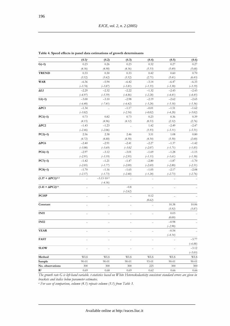

Karsten Staehr Reforms and Economic Growth in Transition Economies
Available online at httpeacesliucit
197
62 Divergence from trend reform path We construct a variable that directly reflects the speed of reforms based on a
suggestion in Berg et al (1999) The idea is to calculate the trend reform level during a fixed time window and then compare the actual reform level with the calculated trend value during the early part of the window The higher the early reform level is above trend level the speedier the implementation of reforms
The implementation speed of broad-based reforms is considered within a four-year window We follow the convention in econometrics and use no time indication of the current realisation of a variable We use τ to indicate years from current year Thus τ = 0 indicates the current year τ = ndash1 indicates a one year lag τ = ndash2 indicates a two year lag etc With this notation the contemporaneous reform level is PC1 and the reform level in year τ ie the reform level lagged τ years is PC1(τ)
We consider a four-year window preceding the current year The total change in the reform index during the four year period is [PC1 ndash PC1(ndash4)] and the average annual change is [PC1 ndash PC1(ndash4)]4 Accordingly the expected trend reform level for any year in the four-year window preceding the current year is
EPC1(τ) = PC1(ndash4) + (4 + τ)middot[PC1 ndash PC1(ndash4)]4 where τ = ndash4 hellip ndash1 For τ = ndash4 EPC1(τ) = PC1(τ) while EPC1(τ) increases
linearly with the annual rate of reform change for τ = ndash3 ndash2 ndash1 The speed variable PC1SP is the sum of the differences between the actual and the trend reform level for years τ = ndash3 and τ = ndash2
PC1SP = [PC1(ndash3) ndash EPC1(ndash3)] + [PC1(ndash2) ndash EPC1(ndash2)] PC1SP is added to specification (31) with the result shown in column (44) in
Table 4 Note that the sample period has changed as PC1SP absorbs three years of the sample The parameter to PC1SP is positive but insignificant31 It should be noted however that the regression contains many variables which could make it difficult for PC1SP to attain significance The partial correlation between G and PC1SP is positive and highly significant Still experiments with different samples non-linear transformations and lagged values of PC1SP show that no stable relationship exists On the suspicion of asymmetric effects we split PC1SP into two variables respectively containing positive and negative values but the results (not shown) were again inconclusive Similar exercises using the liberalisation cluster (PC2) fail to yield any consistent results
63 Scoring of reform speed
Finally we apply methods derived from Wolf (1999) to test for speed effects Initially the number of years from the start of the reform process (ie year 0 using
31 The parameter to ∆PC1 is now insignificant This is the consequence of the shorter sample (also see
(39) in Table 3) and the exclusion of PC1SP
198
EJCE vol 2 n 2 (2005)
Available online at httpeacesliucit
transition time) until PC1 has increased by 4 is counted32 This number (score) would be eg 2 for the Czech Republic and Estonia 4 for Hungary and Moldova and 7 for Bulgaria and Croatia For some countries eg Belarus and Macedonia PC1 does not increase by 4 units within by 2001
The variable YEAR is constructed as follows For 1989-1997 it contains zeros for 1998-2001 it contains the speed score provided the score is less than 8 otherwise zero The construction of YEAR with zeros until 1998 implies that only medium-term effects of the speed score are captured and ensures that the measure of reform speed does not affect growth before reforms are actually implemented33
We include YEAR in regression (35) with a constant term and controls for initial conditions (Fixed effects estimation cannot be used when YEAR is included) The result is shown in column (45) in Table 4 The estimated parameter is negative and significant indicating that reform speed is positively correlated with growth ie rapid reform is associated with higher medium-term growth
Another test separates the transition countries into three groups The first group consists of countries undertaking fast reforms (YEAR le 3) the second group consists of countries undertaking gradual reforms (4 le YEAR le 7) and the third group contains reform-resistant laggards (YEAR ge 8) The dummy FAST has zeros for 1989-97 and ones for 1998-2001 for all countries in the first group The dummy SLOW has zeros for 1989-97 and ones for countries in the second group Column (46) in Table 4 shows the result of adding these two dummy variables to regression (35) Both have negative (and significant) parameters The parameter to FAST is smaller than to SLOW which may indicate that slow reforms were beneficial to growth However the Wald test cannot reject the hypothesis that the two parameters are identical
The method of directly inserting the variables YEAR or FAST and SLOW into the growth regression did not provide firm evidence on the effect of speed However there is no evidence that speedy reforms hampered medium-term growth
64 Discussion
Early reforms allow more years in which the transition country can reap the benefits Beyond this trivial finding the panel data methodology employed in this paper does not provide strong arguments for or against rapid reform The short-term cost of reforms might be larger when implemented in bulk but the effect is small and insignificant The medium-term growth effects of rapid reform are uncertain but rapid reforms appear unlikely to hamper growth In sum the speed of reforms does not appear to a quantitatively substantial impact on growth over and above the level effect This result is in conflict with the conclusions in World Bank (1996) and Berg et al (1999) but is broadly in line with Wolf (1999)
32 For a country starting with all reform indices at their lowest level (eg most countries emerging from
the Soviet Union) an increase of PC1 equal to 4 signifies that the country is halfway to a well-developed market economy
33 It also implies that the variable YEAR only contributes to explaining growth in the last four years of the sample 1990-2001 ie the part of the sample where the other right-hand variables are relative less effective
Karsten Staehr Reforms and Economic Growth in Transition Economies
Available online at httpeacesliucit
199
7 Final comments
A novel feature of this paper was the use of principal component clustering of the EBRD reform indices to infer the structure of reform in transition economies A cluster of synchronised broad-based reforms ie liberalisation privatisation and structural reforms covers 795 of all variation in the initial EBRD reform indices A cluster of liberalisation and small-scale reforms without other reforms explains 79 of the variation while six other clusters of unsynchronised reforms span the remaining 126
The growth regressions included the reform clusters inflation terms and control variables As in most other studies inflation was found to be detrimental to growth Synchronised broad-based reforms had a positive impact on growth in the medium term with a negative short-term effect at the early stages of reform Also a policy of liberalisation and small-scale privatisation without accompanying structural reforms were shown to have a positive effect (again with a possible early negative short-term effect) Accelerated large-scale privatisation without small-scale privatisation and structural reforms were found likely to harm growth both in the short and the medium term
Conversely small-scale privatisation without large-scale privatisation appears beneficial to growth A less certain result is that market opening and price liberalisation without accompanying privatisation and enterprise reforms appear correlated with lower growth but this effect stems primarily for the most recent period Reversing this result privatisation and restructuring without market opening may be good for growth Finally bank liberalisation without enterprise restructuring might be harmful while enterprise reforms without bank liberalisation may increase growth
Effects from the speed of reforms are mostly absent with the exception that early reforms leave the transition country a longer period in which to reap the benefits of reforms Possible negative short-term effects of rapid reforms are likely to be modest and could be balanced by possible positive medium-term effects The broad overall conclusion is that speed per se has no discernible impact on growth
Finally what can we now say about the three questions raised in the introduction
First the analysis revealed a complex pattern of reform complementarities with notable implications for the sequencing of reforms Balanced wide-ranging reforms based on simultaneous progress in liberalisation privatisation and structural reforms are favourable to growth and hence suggest a mutually reinforcing effect of various reform elements
Liberalisation combined with small-scale privatisation is beneficial even in the absence of other reforms In this case unsynchronised reforms produce positive growth effects Thus liberalisation and small-scale privatisation are not perfectly complementary to deeper reforms such as large-scale privatisation and structural reforms A sequenced reform policy that stresses liberalisation and small-scale privatisation is beneficial Early ldquoeasyrdquo reforms should therefore not be postponed in the absence of a comprehensive reform strategy
A number of unsynchronised reform packages proved detrimental to growth Sequenced policy packages involving large-scale privatisation without small-scale privatisation market opening without accompanying reforms and bank liberalisation without enterprise restructuring lead to lower growth in the short andor medium term Conversely a ldquoreversalrdquo of the policy mix would produce packages beneficial to growth
200
EJCE vol 2 n 2 (2005)
Available online at httpeacesliucit
In sum the statistically significant parameters to a number of unsynchronised reform clusters support the view that reforms need to be fine-tuned to take into account complex interactions among reforms
Second we asked which reforms are of foremost importance Within the set of variables used in this paper and using a broad brush a number of variables stand out Inflation stabilisation repeatedly proved important Price liberalisation small-scale privatisation enterprise restructuring (and to a lesser degree trade opening) were generally important in many different combinations with other reforms Large-scale privatisation financial sector reforms and market regulation mainly proved beneficial when they were part of a larger more comprehensive reform packages These results seem to support the view that reform policies are crucial minus even countries that fail to attempt deep structural changes can gain from reforms These findings are broadly in line with the findings in Havrylyshyn and van Rooden (2000) As a caveat we note that only a few variables included in our analysis reflect currently popular themes such as institutional quality and social capital
Third the finding that speed per se is of little importance for growth seems to favour relatively rapid implementation of reforms due to the level effect However this finding also implies there is no direct loss from slowing reforms when it is necessary to get content or sequencing right
These results probably disappoint supporters of big-bang as well as supporters of gradualism as they provide no unequivocal support for either view If it is any consolation to the gradualists reform sequencing appears to be important and reforms should preferably progress synchronously Certain sequenced reform paths are clearly counterproductive Likewise for the big-bang supporters initial phase reforms are beneficial even in the absence of deeper reforms Moreover fast reforms appear generally beneficial Thus there is no clear-cut transition strategy that provides the best results for countries endeavouring to convert a centrally planned economy into a market economy There are only policy choices minus some better than others minus and certain strategies that should be avoided
References
Ahrens J Meurers M (2002) lsquoHow Governance Affects the Quality of Policy Reform and Economic Performance New Evidence for Economies in Transitionrsquo Journal for Institutional Innovation Development and Transition 6 35-56
Aslund A (2002) Building Capitalism The Transformation of the Former Soviet Bloc Cambridge University Press Cambridge
Aziz J Wescott R (1997) lsquoPolicy Complementarities and the Washington Consensusrsquo IMF Working Paper No118
Beck T Levine R (2004) lsquoStock Markets Banks and Growth Panel Evidencersquo Journal of Banking and Finance 28 423-442
Berg A Borensztein E Sahay R Zettelmeyer J (1999) lsquoThe Evolution of Output in the Transition Economies Explaining the Differencesrsquo IMF Working Paper No73
Blanchard O Dornbusch R Krugman P Layard R Summers L (1991) Reform in Eastern Europe MIT Press Cambridge MA
Campos N Coricelli F (2002) lsquoGrowth in Transition What We Know What We Donrsquot and What We Shouldrsquo Journal of Economic Literature 90 793-836
Karsten Staehr Reforms and Economic Growth in Transition Economies
Available online at httpeacesliucit
201
Correa R (2002) lsquoThe Washington Consensus in Latin America A Quantitative Evaluationrsquo mimeo San Francisco de Quito University Ecuador
Crafts N (2000) lsquoGlobalization and Growth in the Twentieth Centuryrsquo in Prasad E (ed) Supporting Studies for the World Economic Outlook International Monetary Fund Washington DC
de Melo M Denizer C Gelb A (1997) lsquoFrom Plan to Market Patterns of Transitionrsquo in Blejer M Skreb M (eds) Macroeconomic Stabilization in Transition Economies Cambridge University Press Cambridge
de Melo M Denizer C Gelb A (2001) lsquoCircumstance and Choice The Role of Initial Conditions and Policies in Transition Economiesrsquo World Bank Economic Review 15 1-31
Djankov S Murrell P (2002) lsquoEnterprise Restructuring in Transition A Quantitative Surveyrsquo Journal of Economic Literature 90 739-792
EBRD (1999-2004) Transition Report European Bank for Reconstruction and Development Fidrmuc J (2003) lsquoEconomic Reform Democracy and Growth during Post Communist
Transitionrsquo European Journal of Political Economy 19 583-604 Fischer S Gelb A (1991) lsquoThe Process of Socialist Economic Transformationrsquo Journal of
Economic Perspectives 5 91-105 Fischer S Sahay R (2000) lsquoThe Transition Economies After Ten Yearsrsquo IMF Working Paper
No30 Fischer S Sahay R Vegh C (1996a) lsquoStabilization and Growth in Transition Economies The
Early Experiencersquo Journal of Economic Perspectives 10 45-66 Fischer S Sahay R Vegh C (1996b) lsquoEconomies in Transition The Beginnings of Growthrsquo
American Economic Review 86 229-233 Havrylyshyn O van Rooden R (2000) lsquoInstitutions Matter in Transition but so do Policiesrsquo
IMF Working Paper No70 Havrylyshyn O (2001) lsquoRecovery and Growth in Transition A Decade of Evidencersquo IMF Staff
Paper 48 53-87 Havrylyshyn O Izvorski I van Rooden R (1998) lsquoRecovery and Growth in Transition
Economies 1990-97 A Stylized Regression Analysisrsquo IMF Working Paper No141 Heybey B Murrell P (1999) lsquoThe Relationship Between Economic Growth and the Speed of
Liberalization During the Transitionrsquo Policy Reform 3 121-37 IMF (1997) World Economic Outlook Globalization Opportunities and Challenges May chapter IV IMF (2000) World Economic Outlook Focus on Transition Economies October chapter III Judson R Owen A (1999) lsquoEstimating Dynamic Panel Data Models A Practical Guide for
Macroeconomistsrsquo Economics Letters 65 9-15 Nerlove M (2002) lsquoProperties of Alternative Estimators of Dynamic Panel Models An
Empirical Analysis of Cross-Country Data for the Study of Economic Growthrsquo in Nerlove M Essays in Panel Data Econometrics Cambridge University Press Cambridge
Nsouli S Rached M Funke N (2002) lsquoThe Speed of Adjustment and the Sequencing of Economic Reforms Issues and Guidelines for Policymakersrsquo IMF Working Paper No132
OECD (1998) OECD Economic Surveys Czech Republic May OECD OECD (2000) OECD Economic Surveys Czech Republic February OECD Pattillo C Poirson H Ricca L (2002) lsquoExternal Debt and Growthrsquo IMF Working Paper No69 Radulescu R Barlow D (2002) lsquoThe Relation between Policies and Growth in Transition
Countriesrsquo Economics of Transition 10 719-745 Roland G (2001) lsquoTen Years After hellip Transition and Economicsrsquo IMF Staff Papers 48 29-52
202
EJCE vol 2 n 2 (2005)
Available online at httpeacesliucit
Sachs J Zinnes G Eilat Y (2000) lsquoPatterns of Economic Reform and its Determinants in Transition Economies 1990-1998rsquo Harvard Institute for International Development CAER II Discussion Paper No 61
Staehr K (2003) lsquoReforms and Economic Growth in Transition Economies Complementarity Sequencing and Speedrsquo BOFIT Discussion Paper No1
Stiglitz J (2001) lsquoWhither Reform Ten Years of Transitionrsquo in Pleskovic B Stiglitz J (eds) World Bank Annual Bank Conference on Development Economics 1999 World Bank Washington DC
Wacziarg R (2002) lsquoReview of Easterlyrsquos The Elusive Quest for Growthrsquo Journal of Economic Literature 90 907-918
Wolf H (1999) lsquoTransition Strategies Choices and Outcomesrsquo Princeton Studies in International Finance No85
World Bank (1996) World Development Report 1996 From Plan to Market World Bank Washington DC
World Bank (2002) Transition The First Ten Years Analysis and Lessons for Eastern Europe and the former Soviet Union World Bank Washington DC
Zinnes C Eilat Y Sachs J (2001) lsquoThe Gains from Privatization in Transition Economies Is lsquoChange of Ownershiprsquo Enoughrsquo IMF Staff Papers 48 146-169
Karsten Staehr Reforms and Economic Growth in Transition Economies
Available online at httpeacesliucit
199
7 Final comments
A novel feature of this paper was the use of principal component clustering of the EBRD reform indices to infer the structure of reform in transition economies A cluster of synchronised broad-based reforms ie liberalisation privatisation and structural reforms covers 795 of all variation in the initial EBRD reform indices A cluster of liberalisation and small-scale reforms without other reforms explains 79 of the variation while six other clusters of unsynchronised reforms span the remaining 126
The growth regressions included the reform clusters inflation terms and control variables As in most other studies inflation was found to be detrimental to growth Synchronised broad-based reforms had a positive impact on growth in the medium term with a negative short-term effect at the early stages of reform Also a policy of liberalisation and small-scale privatisation without accompanying structural reforms were shown to have a positive effect (again with a possible early negative short-term effect) Accelerated large-scale privatisation without small-scale privatisation and structural reforms were found likely to harm growth both in the short and the medium term
Conversely small-scale privatisation without large-scale privatisation appears beneficial to growth A less certain result is that market opening and price liberalisation without accompanying privatisation and enterprise reforms appear correlated with lower growth but this effect stems primarily for the most recent period Reversing this result privatisation and restructuring without market opening may be good for growth Finally bank liberalisation without enterprise restructuring might be harmful while enterprise reforms without bank liberalisation may increase growth
Effects from the speed of reforms are mostly absent with the exception that early reforms leave the transition country a longer period in which to reap the benefits of reforms Possible negative short-term effects of rapid reforms are likely to be modest and could be balanced by possible positive medium-term effects The broad overall conclusion is that speed per se has no discernible impact on growth
Finally what can we now say about the three questions raised in the introduction
First the analysis revealed a complex pattern of reform complementarities with notable implications for the sequencing of reforms Balanced wide-ranging reforms based on simultaneous progress in liberalisation privatisation and structural reforms are favourable to growth and hence suggest a mutually reinforcing effect of various reform elements
Liberalisation combined with small-scale privatisation is beneficial even in the absence of other reforms In this case unsynchronised reforms produce positive growth effects Thus liberalisation and small-scale privatisation are not perfectly complementary to deeper reforms such as large-scale privatisation and structural reforms A sequenced reform policy that stresses liberalisation and small-scale privatisation is beneficial Early ldquoeasyrdquo reforms should therefore not be postponed in the absence of a comprehensive reform strategy
A number of unsynchronised reform packages proved detrimental to growth Sequenced policy packages involving large-scale privatisation without small-scale privatisation market opening without accompanying reforms and bank liberalisation without enterprise restructuring lead to lower growth in the short andor medium term Conversely a ldquoreversalrdquo of the policy mix would produce packages beneficial to growth
200
EJCE vol 2 n 2 (2005)
Available online at httpeacesliucit
In sum the statistically significant parameters to a number of unsynchronised reform clusters support the view that reforms need to be fine-tuned to take into account complex interactions among reforms
Second we asked which reforms are of foremost importance Within the set of variables used in this paper and using a broad brush a number of variables stand out Inflation stabilisation repeatedly proved important Price liberalisation small-scale privatisation enterprise restructuring (and to a lesser degree trade opening) were generally important in many different combinations with other reforms Large-scale privatisation financial sector reforms and market regulation mainly proved beneficial when they were part of a larger more comprehensive reform packages These results seem to support the view that reform policies are crucial minus even countries that fail to attempt deep structural changes can gain from reforms These findings are broadly in line with the findings in Havrylyshyn and van Rooden (2000) As a caveat we note that only a few variables included in our analysis reflect currently popular themes such as institutional quality and social capital
Third the finding that speed per se is of little importance for growth seems to favour relatively rapid implementation of reforms due to the level effect However this finding also implies there is no direct loss from slowing reforms when it is necessary to get content or sequencing right
These results probably disappoint supporters of big-bang as well as supporters of gradualism as they provide no unequivocal support for either view If it is any consolation to the gradualists reform sequencing appears to be important and reforms should preferably progress synchronously Certain sequenced reform paths are clearly counterproductive Likewise for the big-bang supporters initial phase reforms are beneficial even in the absence of deeper reforms Moreover fast reforms appear generally beneficial Thus there is no clear-cut transition strategy that provides the best results for countries endeavouring to convert a centrally planned economy into a market economy There are only policy choices minus some better than others minus and certain strategies that should be avoided
References
Ahrens J Meurers M (2002) lsquoHow Governance Affects the Quality of Policy Reform and Economic Performance New Evidence for Economies in Transitionrsquo Journal for Institutional Innovation Development and Transition 6 35-56
Aslund A (2002) Building Capitalism The Transformation of the Former Soviet Bloc Cambridge University Press Cambridge
Aziz J Wescott R (1997) lsquoPolicy Complementarities and the Washington Consensusrsquo IMF Working Paper No118
Beck T Levine R (2004) lsquoStock Markets Banks and Growth Panel Evidencersquo Journal of Banking and Finance 28 423-442
Berg A Borensztein E Sahay R Zettelmeyer J (1999) lsquoThe Evolution of Output in the Transition Economies Explaining the Differencesrsquo IMF Working Paper No73
Blanchard O Dornbusch R Krugman P Layard R Summers L (1991) Reform in Eastern Europe MIT Press Cambridge MA
Campos N Coricelli F (2002) lsquoGrowth in Transition What We Know What We Donrsquot and What We Shouldrsquo Journal of Economic Literature 90 793-836
Karsten Staehr Reforms and Economic Growth in Transition Economies
Available online at httpeacesliucit
201
Correa R (2002) lsquoThe Washington Consensus in Latin America A Quantitative Evaluationrsquo mimeo San Francisco de Quito University Ecuador
Crafts N (2000) lsquoGlobalization and Growth in the Twentieth Centuryrsquo in Prasad E (ed) Supporting Studies for the World Economic Outlook International Monetary Fund Washington DC
de Melo M Denizer C Gelb A (1997) lsquoFrom Plan to Market Patterns of Transitionrsquo in Blejer M Skreb M (eds) Macroeconomic Stabilization in Transition Economies Cambridge University Press Cambridge
de Melo M Denizer C Gelb A (2001) lsquoCircumstance and Choice The Role of Initial Conditions and Policies in Transition Economiesrsquo World Bank Economic Review 15 1-31
Djankov S Murrell P (2002) lsquoEnterprise Restructuring in Transition A Quantitative Surveyrsquo Journal of Economic Literature 90 739-792
EBRD (1999-2004) Transition Report European Bank for Reconstruction and Development Fidrmuc J (2003) lsquoEconomic Reform Democracy and Growth during Post Communist
Transitionrsquo European Journal of Political Economy 19 583-604 Fischer S Gelb A (1991) lsquoThe Process of Socialist Economic Transformationrsquo Journal of
Economic Perspectives 5 91-105 Fischer S Sahay R (2000) lsquoThe Transition Economies After Ten Yearsrsquo IMF Working Paper
No30 Fischer S Sahay R Vegh C (1996a) lsquoStabilization and Growth in Transition Economies The
Early Experiencersquo Journal of Economic Perspectives 10 45-66 Fischer S Sahay R Vegh C (1996b) lsquoEconomies in Transition The Beginnings of Growthrsquo
American Economic Review 86 229-233 Havrylyshyn O van Rooden R (2000) lsquoInstitutions Matter in Transition but so do Policiesrsquo
IMF Working Paper No70 Havrylyshyn O (2001) lsquoRecovery and Growth in Transition A Decade of Evidencersquo IMF Staff
Paper 48 53-87 Havrylyshyn O Izvorski I van Rooden R (1998) lsquoRecovery and Growth in Transition
Economies 1990-97 A Stylized Regression Analysisrsquo IMF Working Paper No141 Heybey B Murrell P (1999) lsquoThe Relationship Between Economic Growth and the Speed of
Liberalization During the Transitionrsquo Policy Reform 3 121-37 IMF (1997) World Economic Outlook Globalization Opportunities and Challenges May chapter IV IMF (2000) World Economic Outlook Focus on Transition Economies October chapter III Judson R Owen A (1999) lsquoEstimating Dynamic Panel Data Models A Practical Guide for
Macroeconomistsrsquo Economics Letters 65 9-15 Nerlove M (2002) lsquoProperties of Alternative Estimators of Dynamic Panel Models An
Empirical Analysis of Cross-Country Data for the Study of Economic Growthrsquo in Nerlove M Essays in Panel Data Econometrics Cambridge University Press Cambridge
Nsouli S Rached M Funke N (2002) lsquoThe Speed of Adjustment and the Sequencing of Economic Reforms Issues and Guidelines for Policymakersrsquo IMF Working Paper No132
OECD (1998) OECD Economic Surveys Czech Republic May OECD OECD (2000) OECD Economic Surveys Czech Republic February OECD Pattillo C Poirson H Ricca L (2002) lsquoExternal Debt and Growthrsquo IMF Working Paper No69 Radulescu R Barlow D (2002) lsquoThe Relation between Policies and Growth in Transition
Countriesrsquo Economics of Transition 10 719-745 Roland G (2001) lsquoTen Years After hellip Transition and Economicsrsquo IMF Staff Papers 48 29-52
202
EJCE vol 2 n 2 (2005)
Available online at httpeacesliucit
Sachs J Zinnes G Eilat Y (2000) lsquoPatterns of Economic Reform and its Determinants in Transition Economies 1990-1998rsquo Harvard Institute for International Development CAER II Discussion Paper No 61
Staehr K (2003) lsquoReforms and Economic Growth in Transition Economies Complementarity Sequencing and Speedrsquo BOFIT Discussion Paper No1
Stiglitz J (2001) lsquoWhither Reform Ten Years of Transitionrsquo in Pleskovic B Stiglitz J (eds) World Bank Annual Bank Conference on Development Economics 1999 World Bank Washington DC
Wacziarg R (2002) lsquoReview of Easterlyrsquos The Elusive Quest for Growthrsquo Journal of Economic Literature 90 907-918
Wolf H (1999) lsquoTransition Strategies Choices and Outcomesrsquo Princeton Studies in International Finance No85
World Bank (1996) World Development Report 1996 From Plan to Market World Bank Washington DC
World Bank (2002) Transition The First Ten Years Analysis and Lessons for Eastern Europe and the former Soviet Union World Bank Washington DC
Zinnes C Eilat Y Sachs J (2001) lsquoThe Gains from Privatization in Transition Economies Is lsquoChange of Ownershiprsquo Enoughrsquo IMF Staff Papers 48 146-169
Related Documents