Refined error analysis in second-order Sigma-Delta modulation with constant inputs

Refined error analysis in second order Σ∆

modulation with constant inputs

C. Sinan Gunturk1 and Nguyen T. Thao2

1Courant Institute of Mathematical Sciences, New York University, 251 Mercer Street, New York, NY 10012.

e-mail: [email protected]

2Department of Electrical Engineering, City College and Graduate School, City University of New York, Convent

Avenue at 138th Street, New York, NY 10031. e-mail: [email protected]

This work has been supported in part by the National Science Foundation Grants DMS 97-29992, DMS 02-19053,

DMS 02-19072, CCR 02-09431 and the Francis Robbins Upton fellowship at Princeton University.

August 26, 2003 DRAFT

Truong-Thao Nguyen

IEEE Transactions on Information theory, submitted in March 2001

i

Abstract

Although the technique of sigma-delta (Σ∆) modulation is well established in practice for performing

high resolution analog-to-digital conversion, theoretical analysis of the error between the input signal and

the reconstructed signal has remained partial. For modulators of order higher than 1, the only rigorous

error analysis currently available that matches practical and numerical simulation results is only applicable

to a very special configuration, namely, the standard and ideal k-bit k-loop Σ∆ modulator. Moreover, the

error measure involves averaging over time as well as possibly over the input value. At the second order, it

is known in practice that the mean-squared error decays with the oversampling ratio λ at the rate O(λ−5).

In this paper, we introduce two new fundamental results in this analysis for constant input signals. We

first establish a framework of analysis that is applicable to all second order modulators provided that the

built-in quantizer has uniformly spaced output levels, and that the noise transfer function has its two

zeros at the zero frequency. In particular, this includes the one-bit case, a rigorous and deterministic

analysis of which is still not available. This generalization has been possible thanks to the discovery of

the mathematical tiling property of the state variables of such modulators. The second aspect of our

contribution is to perform an instantaneous error analysis that avoids infinite time-averaging. Until now,

only an O(λ−4) type error bound was known to hold in this setting. Under our generalized framework, we

provide two types of squared-error estimates; one that is statistically averaged over the input and another

that is valid for almost every input (in the sense of Lebesgue measure). In both cases, we improve the

error bound to O(λ−4.5), up to a logarithmic factor, for a general class of modulators including some

specific ones that are covered in this paper in detail. In the particular case of the standard and ideal 2-bit

double-loop configuration, our methods provide a (previously unavailable) instantaneous error bound of

O(λ−5), again up to a logarithmic factor.

Keywords

A/D conversion, Σ∆ modulation, quantization, piecewise affine transformation, tiling, uniform distri-

bution, discrepancy, exponential sums.


ii

Contents

I Introduction 1

II Equations of the second order modulator 7

II-A Feedback equations and an equivalent system . . . . . . . . . . . . . . . . 7

II-B The quantizer . . . . . . . . . . . . . . . . . . . . . . . . . . . . . . . . . . 10

II-C State-space equations . . . . . . . . . . . . . . . . . . . . . . . . . . . . . 10

II-D Basic error analysis . . . . . . . . . . . . . . . . . . . . . . . . . . . . . . 11

II-E Nonlinear functions T . . . . . . . . . . . . . . . . . . . . . . . . . . . . . 14

III Invariant tiles under constant inputs 14

III-A Experimental observation of tiling . . . . . . . . . . . . . . . . . . . . . . 15

III-B Mathematical justifications of tiling . . . . . . . . . . . . . . . . . . . . . 17

III-C The single invariant tile case and its fundamental consequence . . . . . . . 18

III-D Further developments on the single tile case . . . . . . . . . . . . . . . . . 20

IV Thorough study of three particular configurations 22

IV-A Linear T and 2-bit quantizer: the L2 system . . . . . . . . . . . . . . . . . 23

IV-B Linear T and 1-bit quantizer: the L1 system . . . . . . . . . . . . . . . . . 24

IV-C A new rule: Quadratic T and 1-bit quantizer: the Q1 system . . . . . . . 25

IV-D Boundedness, regularity and tiling . . . . . . . . . . . . . . . . . . . . . . 27

V The Main Theorem 28

VI Discussion and further remarks 36

Appendix 37

-A Tools from the theory of uniform distribution . . . . . . . . . . . . . . . . 37

-B Invariant set Γx for the L1 system . . . . . . . . . . . . . . . . . . . . . . . 40

-C Invariant set Γx for the Q1 system . . . . . . . . . . . . . . . . . . . . . . . 42

-D Proof of Proposition IV.1 . . . . . . . . . . . . . . . . . . . . . . . . . . . . 45

-E On the analysis of the quadratic scheme: zero-centroid setting of C(x) . . . 47


1

I. Introduction

In the current state of the art of circuit design, high resolution A/D and D/A conversion

is achieved by oversampling the input signal and transforming it into a sequence of coarsely

quantized values which are selected from a small alphabet consisting of as few as two

symbols. An approximation of the input is then obtained by extracting the in-band content

of the quantized signal via appropriate filtering. Sigma-delta (Σ∆) modulation is a widely

used method for this purpose (see [1], [19], [14]), owing its success largely to its robustness

against circuit imperfections and ease of implementation.

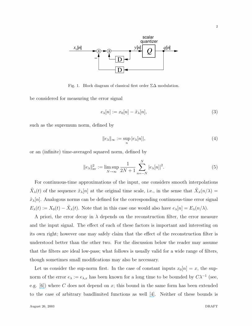
The simplest version of Σ∆ modulation is the single-loop (first order) version originally

introduced in [15], which involves an integrator, a single-bit quantizer and a negative

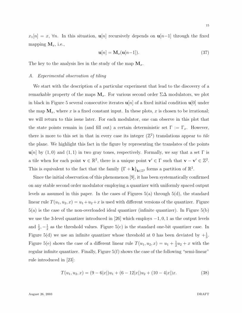
feedback from the quantizer output into the integrator input. The system equations are y[n] = y[n−1] + x0[n]− q[n−1]

q[n] = Q(y[n]).(1)

The block diagram of Figure 1 symbolizes this system. Here, x0[n] = X0(n/λ), n ∈ Z,

denotes the sequence of samples of the continuous-time input signal X0(t) sampled at λ

times per time-unit. We shall normalize the time-unit so that the spacing between the

Nyquist-rate samples is equal to one time-unit; thus λ is also equal to the oversampling

rate. Throughout the paper, λ will be assumed to take integer values. The signals y[n] and

q[n] = Q(y[n]) denote the quantizer input and the output, respectively. In this system, the

quantizer Q is one-bit; i.e., it outputs values from a discrete set consisting of two values,

although multi-bit quantizers are also used in practice, especially for higher order systems.

Unless otherwise specified, the input is assumed to be in [−12, 1

2] when the quantization

step size is normalized to 1.

It is one of the primary objectives of the theory to understand, as a function of λ, the

behavior of the error between the input signal and the approximations given by

xλ[n] := (φλ ∗ q)[n] :=∑

k

φλ[k]q[n−k] (2)

for suitable lowpass filters φλ whose number of taps typically grow linearly in λ, thus

spanning a uniformly bounded duration of real implementation time. Various norms can


https://www.researchgate.net/publication/2987221_A_Unity_Bit_Coding_Method_by_Negative_Feedback?el=1_x_8&enrichId=rgreq-4276f12f34a15f58a8032eece18022b7-XXX&enrichSource=Y292ZXJQYWdlOzMwODUwMjU7QVM6MTIyMTg5NjkzMDY3MjY2QDE0MDYxNDM3MDE5NzM=

https://www.researchgate.net/publication/4377975_Delta-Sigma_Data_Converters_Theory_Design_and_Simulation?el=1_x_8&enrichId=rgreq-4276f12f34a15f58a8032eece18022b7-XXX&enrichSource=Y292ZXJQYWdlOzMwODUwMjU7QVM6MTIyMTg5NjkzMDY3MjY2QDE0MDYxNDM3MDE5NzM=

2

DQ

D

− + +

[ ] [ ]quantizerscalar

y n q nx n0 [ ]

Fig. 1. Block diagram of classical first order Σ∆ modulation.

be considered for measuring the error signal

eλ[n] := x0[n]− xλ[n], (3)

such as the supremum norm, defined by

‖eλ‖∞ := supn|eλ[n]|, (4)

or an (infinite) time-averaged squared norm, defined by

‖eλ‖2av := lim sup

N→∞

1

2N + 1

N∑n=−N

|eλ[n]|2. (5)

For continuous-time approximations of the input, one considers smooth interpolations

Xλ(t) of the sequence xλ[n] at the original time scale, i.e., in the sense that Xλ(n/λ) =

xλ[n]. Analogous norms can be defined for the corresponding continuous-time error signal

Eλ(t) := X0(t)− Xλ(t). Note that in this case one would also have eλ[n] = Eλ(n/λ).

A priori, the error decay in λ depends on the reconstruction filter, the error measure

and the input signal. The effect of each of these factors is important and interesting on

its own right; however one may safely claim that the effect of the reconstruction filter is

understood better than the other two. For the discussion below the reader may assume

that the filters are ideal low-pass; what follows is usually valid for a wide range of filters,

though sometimes small modifications may also be necessary.

Let us consider the sup-norm first. In the case of constant inputs x0[n] = x, the sup-

norm of the error eλ := eλ,x has been known for a long time to be bounded by Cλ−1 (see,

e.g. [6]) where C does not depend on x; this bound in the same form has been extended

to the case of arbitrary bandlimited functions as well [4]. Neither of these bounds is


https://www.researchgate.net/publication/243116654_Approximating_a_bandlimited_function_using_very_coarsely_quantized_data_A_family_of_stable_sigma-delta_modulators_of_arbitrary_order?el=1_x_8&enrichId=rgreq-4276f12f34a15f58a8032eece18022b7-XXX&enrichSource=Y292ZXJQYWdlOzMwODUwMjU7QVM6MTIyMTg5NjkzMDY3MjY2QDE0MDYxNDM3MDE5NzM=

https://www.researchgate.net/publication/3157278_Spectral_Analysis_of_Quantization_Noise_in_a_Single-Loop_Sigma-Delta_Modulator_with_dc_Input?el=1_x_8&enrichId=rgreq-4276f12f34a15f58a8032eece18022b7-XXX&enrichSource=Y292ZXJQYWdlOzMwODUwMjU7QVM6MTIyMTg5NjkzMDY3MjY2QDE0MDYxNDM3MDE5NzM=

3

sharp, however. For constant inputs, one in fact has ‖eλ,x‖∞ ≤ C(x)λ−2+ε for almost

every x (in the sense of Lebesgue measure) where ε > 0 may be arbitrarily small [2],

[8], [10]. Here, the constant C(x) depends on some fine arithmetical properties of x (in

the sense of Diophantine approximations) and is quite irregular (for instance, it is not

square integrable in x on any non-zero interval). For arbitrary bandlimited functions, a

corresponding improvement in the exponent of λ has been found only for the instantaneous

error; for each ε > 0 and each time instant t, one has |Eλ(t)| ≤ C(X ′0(t), ε)λ

−4/3+ε [8],

[10].

It is clear that ‖eλ‖2av ≤ ‖eλ‖2

∞; therefore all upper bounds for the squared sup-norm

apply to the time-averaged squared norm as well. In the first order case with constant

inputs, it turns out that these two norms behave somewhat similarly in the sense that time-

averaging does not yield any significant gain in the exponent of λ and that ‖eλ,x‖2av ≥

c(x)λ−4 for infinitely many λ [24]. This is not the case for the higher order schemes

(which will be defined shortly below) and there still remains a large discrepancy – natural

or artificial – between the best known exponents of λ in the bounds for these two error

norms.

To provide more insight on the size of the error signal, let us now look at the effect

of statistical averaging over the values of the constant input. Various mixed-type error

norms can be considered depending on how one incorporates the mathematical expecta-

tion (taken over the input space) into the norm definition. It is known in the case of

uniformly distributed inputs x that, the mean (expected) time-averaged squared error (or

equivalently, mean-squared time-averaged error) defined by

E(‖eλ,x‖2av) :=

∫ 1/2

−1/2

‖eλ,x‖2av dx (6)

is bounded by Cλ−3 both from above and from below [6]. Note that the sup-norm estimate

Cλ−1, which is uniform for all values of x would yield the suboptimal estimate Cλ−2 for

this quantity; on the other hand, we also see that the constant C(x) in the improved

sup-norm estimate C(x)λ−2+ε cannot be square integrable with respect to x for otherwise

it would yield an impossible Cλ−4+ε type estimate. These remarks apply to the mean-


https://www.researchgate.net/publication/229025654_Improved_Error_Estimates_For_First_Order_Sigma-Delta_Systems?el=1_x_8&enrichId=rgreq-4276f12f34a15f58a8032eece18022b7-XXX&enrichSource=Y292ZXJQYWdlOzMwODUwMjU7QVM6MTIyMTg5NjkzMDY3MjY2QDE0MDYxNDM3MDE5NzM=


https://www.researchgate.net/publication/266002562_Approximating_a_bandlimited_function_using_very_coarsely_quantized_data_Improved_error_estimates_in_sigma-delta_modulation?el=1_x_8&enrichId=rgreq-4276f12f34a15f58a8032eece18022b7-XXX&enrichSource=Y292ZXJQYWdlOzMwODUwMjU7QVM6MTIyMTg5NjkzMDY3MjY2QDE0MDYxNDM3MDE5NzM=



https://www.researchgate.net/publication/2108318_Ergodic_Dynamics_in_Sigma-Delta_Quantization_Tiling_Invariant_Sets_and_Spectral_Analysis_of_Error?el=1_x_8&enrichId=rgreq-4276f12f34a15f58a8032eece18022b7-XXX&enrichSource=Y292ZXJQYWdlOzMwODUwMjU7QVM6MTIyMTg5NjkzMDY3MjY2QDE0MDYxNDM3MDE5NzM=

https://www.researchgate.net/publication/224736154_Time_domain_analysis_of_sigma_delta_modulation?el=1_x_8&enrichId=rgreq-4276f12f34a15f58a8032eece18022b7-XXX&enrichSource=Y292ZXJQYWdlOzMwODUwMjU7QVM6MTIyMTg5NjkzMDY3MjY2QDE0MDYxNDM3MDE5NzM=

4

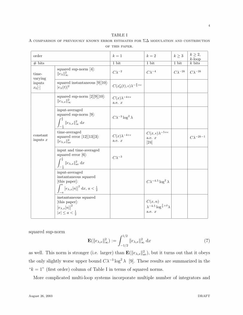
TABLE IA comparison of previously known error estimates for Σ∆ modulation and contribution

of this paper.

order k = 1 k = 2 k ≥ 3 k ≥ 2,k-loop

# bits 1 bit 1 bit 1 bit k bitssquared sup-norm [4]:‖eλ‖2∞ Cλ−2 Cλ−4 Cλ−2k Cλ−2k

time-varyinginputsx0[·]

squared instantaneous [9][10]:|eλ(t)|2 C(x′0(t), ε)λ

− 83+ε

squared sup-norm [2][9][10]:‖eλ,x‖2∞

C(x)λ−4+ε

a.e. x

input-averagedsquared sup-norm [9]:∫ 1

2

− 12

‖eλ,x‖2∞ dx

Cλ−3 log2 λ

constantinputs x

time-averagedsquared error [12][13][3]:‖eλ,x‖2av

C(x)λ−4+ε

a.e. x

C(x, ε)λ−5+ε

a.e. x[24]

Cλ−2k−1

input and time-averagedsquared error [6]:∫ 1

2

− 12

‖eλ,x‖2av dx

Cλ−3

input-averagedinstantaneous squared[this paper]:∫ a

−a

∣∣eλ,x[n]∣∣2 dx, a < 1

2

Cλ−4.5 log2 λ

instantaneous squared[this paper]:∣∣eλ,x[n]

∣∣2|x| ≤ a < 1

2

C(x, n)λ−4.5 log

72+δλ

a.e. x

squared sup-norm

E(‖eλ,x‖2∞) :=

∫ 1/2

−1/2

‖eλ,x‖2∞ dx (7)

as well. This norm is stronger (i.e. larger) than E(‖eλ,x‖2av), but it turns out that it obeys

the only slightly worse upper bound Cλ−3 log2 λ [9]. These results are summarized in the

“k = 1” (first order) column of Table I in terms of squared norms.

More complicated multi-loop systems incorporate multiple number of integrators and


5

feedbacks, and achieve better system performance as λ is increased [12], [13], [3]. For

a k-th order system, the corresponding system equations involve a k-th order difference

equation, which may be presented in the prototypical form

∆ky[n] = x0[n]− q[n], (8)

where ∆k denotes the k-fold composition of the standard difference operator ∆ defined by

∆y[n] = y[n]−y[n−1], and q[n] again represents the Σ∆ quantized output signal (possibly

up to a shift in time). In the case of a k-th order stable Σ∆ modulator (one for which

y[n] is bounded), it is proved in [4] that ‖eλ‖2∞ ≤ Cλ−2k where the constant C is uniform

over the input. They also give the first infinite family of arbitrarily high order single-bit

schemes that are unconditionally stable for arbitrary bounded inputs. Since the sup-norm

is the strongest norm among all the norms we consider, an O(λ−2k) type estimate applies,

in particular, to all the mean-squared norms; however, similar to the first order case, this

does not necessarily reflect the optimal behavior of these systems. Indeed, it is known for

the multi-bit multi-loop configuration with constant inputs that ‖eλ‖2av has an O(λ−2k−1)

type decay [13]. However, note that the analysis of [13] is restricted to only a special case

of Σ∆ modulation with a fixed uniform k-bit quantizer1 for a k-th order scheme. While

using this multi-bit quantizer avoids overloading and eases the analysis of the quantization

error significantly, it is clearly a non-ideal setup for large k, since one of the appeals of

Σ∆ modulation is its capability of working with single-bit quantizers, producing one bit

per input sample.

In this paper, we allow more general quantizers, including single-bit quantizers. As one

important contribution, we analyze Σ∆ schemes for which no better estimate than the one

provided by [4] could previously be given. This includes the remaining “1-bit” columns in

Table I. Under our generalized framework, we provide two types of squared instantaneous

error estimates. The first one involves statistical averaging over the input and is uniform

in time, measured by the sup-norm in time of the mean-squared instantaneous error

∥∥E(e2λ,x[·])

∥∥∞ := sup

n

∫I

|eλ,x[n]|2 dx, (9)

1By this, we mean that the quantizer has uniformly spaced 2k output values and each threshold level is the

midpoint of an interval defined by these output values.


https://www.researchgate.net/publication/220685911_Multiloop_Sigma-Delta_Quantization?el=1_x_8&enrichId=rgreq-4276f12f34a15f58a8032eece18022b7-XXX&enrichSource=Y292ZXJQYWdlOzMwODUwMjU7QVM6MTIyMTg5NjkzMDY3MjY2QDE0MDYxNDM3MDE5NzM=




6

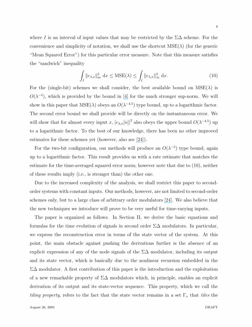
where I is an interval of input values that may be restricted by the Σ∆ scheme. For the

convenience and simplicity of notation, we shall use the shortcut MSE(λ) (for the generic

“Mean Squared Error”) for this particular error measure. Note that this measure satisfies

the “sandwich” inequality∫I

‖eλ,x‖2av dx ≤ MSE(λ) ≤

∫I

‖eλ,x‖2∞ dx. (10)

For the (single-bit) schemes we shall consider, the best available bound on MSE(λ) is

O(λ−4), which is provided by the bound in [4] for the much stronger sup-norm. We will

show in this paper that MSE(λ) obeys an O(λ−4.5) type bound, up to a logarithmic factor.

The second error bound we shall provide will be directly on the instantaneous error. We

will show that for almost every input x, |eλ,x[n]|2 also obeys the upper bound O(λ−4.5) up

to a logarithmic factor. To the best of our knowledge, there has been no other improved

estimates for these schemes yet (however, also see [24]).

For the two-bit configuration, our methods will produce an O(λ−5) type bound, again

up to a logarithmic factor. This result provides us with a rate estimate that matches the

estimate for the time-averaged squared error norm; however note that due to (10), neither

of these results imply (i.e., is stronger than) the other one.

Due to the increased complexity of the analysis, we shall restrict this paper to second-

order systems with constant inputs. Our methods, however, are not limited to second-order

schemes only, but to a large class of arbitrary order modulators [24]. We also believe that

the new techniques we introduce will prove to be very useful for time-varying inputs.

The paper is organized as follows. In Section II, we derive the basic equations and

formulas for the time evolution of signals in second order Σ∆ modulators. In particular,

we express the reconstruction error in terms of the state vector of the system. At this

point, the main obstacle against pushing the derivations further is the absence of an

explicit expression of any of the node signals of the Σ∆ modulator, including its output

and its state vector, which is basically due to the nonlinear recursion embedded in the

Σ∆ modulator. A first contribution of this paper is the introduction and the exploitation

of a new remarkable property of Σ∆ modulators which, in principle, enables an explicit

derivation of its output and its state-vector sequence. This property, which we call the

tiling property, refers to the fact that the state vector remains in a set Γx that tiles the





7

+ +

Ddelay

DQ

D

- - + +

[ ] [ ]

xx βα

quantizerscalar

0[ ]x n y n q n

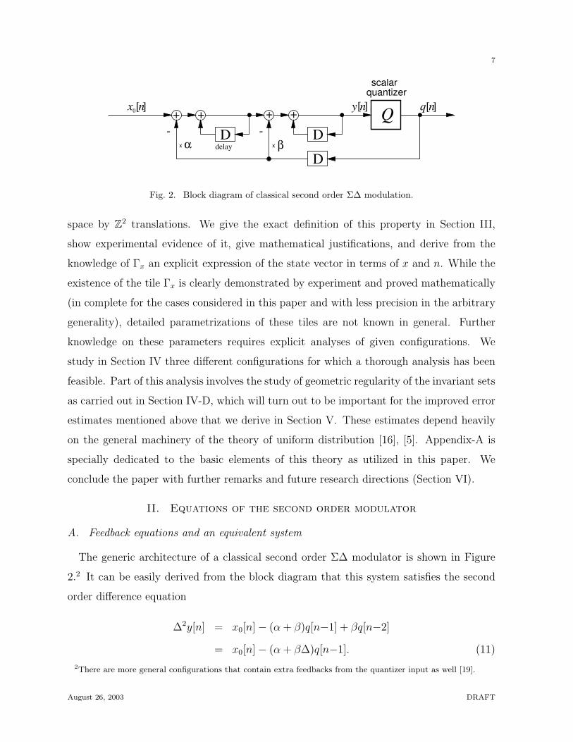
Fig. 2. Block diagram of classical second order Σ∆ modulation.

space by Z2 translations. We give the exact definition of this property in Section III,

show experimental evidence of it, give mathematical justifications, and derive from the

knowledge of Γx an explicit expression of the state vector in terms of x and n. While the

existence of the tile Γx is clearly demonstrated by experiment and proved mathematically

(in complete for the cases considered in this paper and with less precision in the arbitrary

generality), detailed parametrizations of these tiles are not known in general. Further

knowledge on these parameters requires explicit analyses of given configurations. We

study in Section IV three different configurations for which a thorough analysis has been

feasible. Part of this analysis involves the study of geometric regularity of the invariant sets

as carried out in Section IV-D, which will turn out to be important for the improved error

estimates mentioned above that we derive in Section V. These estimates depend heavily

on the general machinery of the theory of uniform distribution [16], [5]. Appendix-A is

specially dedicated to the basic elements of this theory as utilized in this paper. We

conclude the paper with further remarks and future research directions (Section VI).

II. Equations of the second order modulator

A. Feedback equations and an equivalent system

The generic architecture of a classical second order Σ∆ modulator is shown in Figure

2.2 It can be easily derived from the block diagram that this system satisfies the second

order difference equation

∆2y[n] = x0[n]− (α + β)q[n−1] + βq[n−2]

= x0[n]− (α + β∆)q[n−1]. (11)

2There are more general configurations that contain extra feedbacks from the quantizer input as well [19].


8

In the standard case of the double-loop configuration studied in [13] where α = β = 1,

this equation can be rewritten as a difference equation for the quantizer error y[n]− q[n]:

∆2(y[n]− q[n]) = x0[n]− q[n]. (12)

In the general case, the direct signal analysis of the system of Figure 2 is difficult due to

the complicated action of the feedback. We shall first derive an equivalent diagram of this

system which yields simpler feedback mechanisms. Consider the change of input variable

defined by the difference equation

x0[n] = γ∆2x1[n] + (α + β∆)x1[n−1] (13)

where γ is a parameter to be chosen at our disposal. Next, define the auxiliary variables

u1[n] and u2[n] to satisfy the difference equations

∆u2[n] = u1[n]; ∆u1[n] = x1[n]− q[n]. (14)

Then, by subsequently applying (14), (11) and (13), it follows that

∆2(αu2[n−1] + βu1[n−1] + γx1[n]) = (α + β∆)(x1[n−1]− q[n−1]) + γ∆2x1[n]

= (α + β∆)x1[n−1] + ∆2y[n]− x0[n] + γ∆2x1[n]

= ∆2y[n]. (15)

Assuming that the initial conditions for x1[n] have been picked (arbitrarily, or by some

criterion), the initial conditions for the sequences u1[n] and u2[n] can now be chosen so

that (15) implies

y[n] = βu1[n−1] + αu2[n−1] + γx1[n]

= T (u1[n−1], u2[n−1], x1[n]) , (16)

where

T (u1, u2, x) := βu1 + αu2 + γx. (17)

Since

q[n] = Q(y[n]), (18)



9

1

1

1

1

1

2

2

1

2

[ ]

[ ]D

D u

u n

n[ ] [ −1]

u n

u n

operatormemoryless

Qquantizerscalar

y n q n[ ][ ]

x n

u n

[ −1]

u n

u n

[ ]

[ −1]

[ −1]D

[ ]

[ ]+

uDu nq n

+ +n

[ −1]

x nT

[ ]

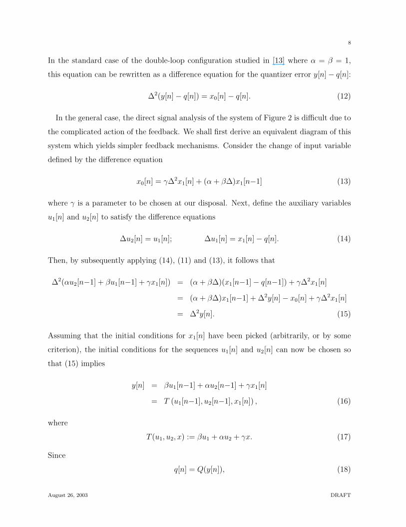
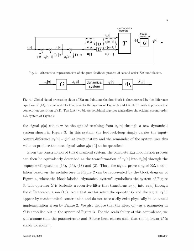
Fig. 3. Alternative representation of the pure feedback process of second order Σ∆ modulation.

dynamicalsystem

[ ] [ ][ ] [ ]x nx n G Φq n0 1 x nλ

λ

~

Fig. 4. Global signal processing chain of Σ∆ modulation: the first block is characterized by the difference

equation of (13), the second block represents the system of Figure 3 and the third block represents the

convolution operation of (2). The first two blocks combined together generalizes the original second order

Σ∆ system of Figure 2.

the signal y[n] can now be thought of resulting from x1[n] through a new dynamical

system shown in Figure 3. In this system, the feedback-loop simply carries the input-

output difference x1[n] − q[n] at every instant and the remainder of the system uses this

value to produce the next signal value y[n+1] to be quantized.

Given the construction of this dynamical system, the complete Σ∆ modulation process

can then be equivalently described as the transformation of x0[n] into xλ[n] through the

sequence of equations (13), (16), (18) and (2). Thus, the signal processing of Σ∆ modu-

lation based on the architecture in Figure 2 can be represented by the block diagram of

Figure 4, where the block labeled “dynamical system” symbolizes the system of Figure

3. The operator G is basically a recursive filter that transforms x0[n] into x1[n] through

the difference equation (13). Note that in this setup the operator G and the signal x1[n]

appear by mathematical construction and do not necessarily exist physically in an actual

implementation given by Figure 2. We also deduce that the effect of γ as a parameter in

G is cancelled out in the system of Figure 3. For the realizability of this equivalence, we

will assume that the parameters α and β have been chosen such that the operator G is

stable for some γ.


10

Let us note at this stage that while the Σ∆ modulator described by Figure 2 is favorable

for the efficiency of its circuit implementation, it is also a legitimate option to switch to

the slightly less efficient Σ∆ modulator scheme described solely by Figure 3 (i.e. without

the pre-filter G) when circuit implementation is not the primary concern. In this case,

γ would be an additional parameter of design. In fact there would be a whole range of

flexibility in the choice of T if nonlinear functions are also allowed. We shall return to this

issue in Section II-E.

B. The quantizer

We assume in this paper that the quantizer Q is uniform of step size 1, in the sense

that its output values are of the type i − 12

where i = i0, i0 + 1, ..., i1. The quantization

intervals I i which satisfy Q(I i) = i− 12

are defined by

I i :=

(−∞, i0), i = i0,

[i− 1, i), i0 < i < i1,

[i1 − 1, +∞), i = i1

(19)

We call the quantizer k-bit if i1 − i0 + 1 = 2k. In the particular one-bit case, we assume

that i0 = 0, so that the quantizer mapping reduces to

Q(y) =

−12, if y < 0,

+12, if y ≥ 0.

(20)

We call the quantizer infinite if i0 = −∞ and i1 = +∞.

We say that the quantizer is overloaded if |y−Q(y)| > 12. Note that the infinite quantizer

is never overloaded.

C. State-space equations

At every instant, u1[n] and u2[n] constitute the state variables of the system. We will

use the short hand notation

u[n] =

u1[n]

u2[n]

(21)


11

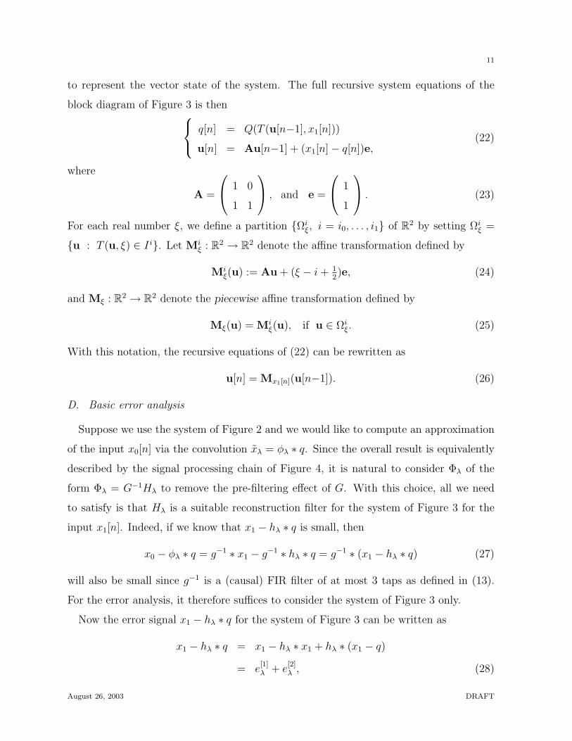
to represent the vector state of the system. The full recursive system equations of the

block diagram of Figure 3 is then q[n] = Q(T (u[n−1], x1[n]))

u[n] = Au[n−1] + (x1[n]− q[n])e,(22)

where

A =

1 0

1 1

, and e =

1

1

. (23)

For each real number ξ, we define a partition Ωiξ, i = i0, . . . , i1 of R2 by setting Ωi

ξ =

u : T (u, ξ) ∈ I i. Let Miξ : R2 → R2 denote the affine transformation defined by

Miξ(u) := Au + (ξ − i + 1

2)e, (24)

and Mξ : R2 → R2 denote the piecewise affine transformation defined by

Mξ(u) = Miξ(u), if u ∈ Ωi

ξ. (25)

With this notation, the recursive equations of (22) can be rewritten as

u[n] = Mx1[n](u[n−1]). (26)

D. Basic error analysis

Suppose we use the system of Figure 2 and we would like to compute an approximation

of the input x0[n] via the convolution xλ = φλ ∗ q. Since the overall result is equivalently

described by the signal processing chain of Figure 4, it is natural to consider Φλ of the

form Φλ = G−1Hλ to remove the pre-filtering effect of G. With this choice, all we need

to satisfy is that Hλ is a suitable reconstruction filter for the system of Figure 3 for the

input x1[n]. Indeed, if we know that x1 − hλ ∗ q is small, then

x0 − φλ ∗ q = g−1 ∗ x1 − g−1 ∗ hλ ∗ q = g−1 ∗ (x1 − hλ ∗ q) (27)

will also be small since g−1 is a (causal) FIR filter of at most 3 taps as defined in (13).

For the error analysis, it therefore suffices to consider the system of Figure 3 only.

Now the error signal x1 − hλ ∗ q for the system of Figure 3 can be written as

x1 − hλ ∗ q = x1 − hλ ∗ x1 + hλ ∗ (x1 − q)

= e[1]λ + e

[2]λ , (28)


12

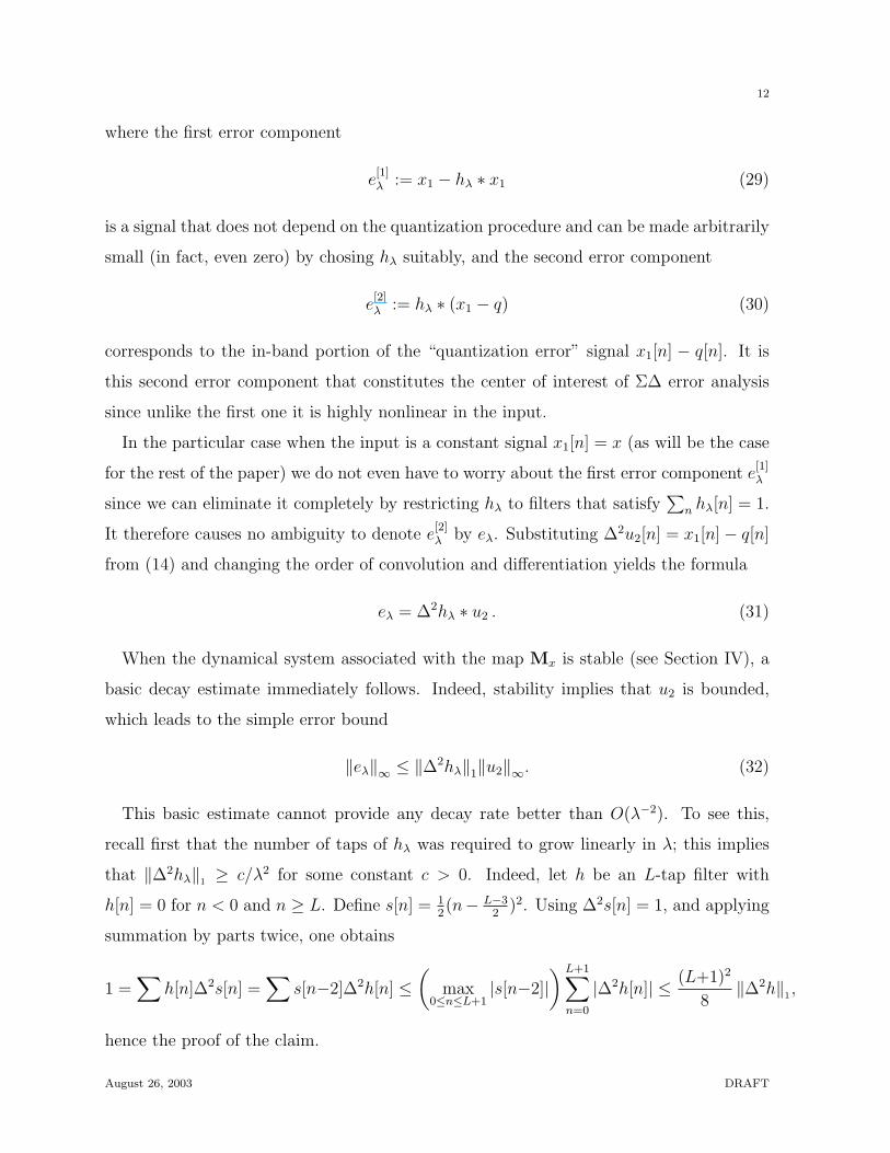
where the first error component

e[1]λ := x1 − hλ ∗ x1 (29)

is a signal that does not depend on the quantization procedure and can be made arbitrarily

small (in fact, even zero) by chosing hλ suitably, and the second error component

e[2]λ := hλ ∗ (x1 − q) (30)

corresponds to the in-band portion of the “quantization error” signal x1[n] − q[n]. It is

this second error component that constitutes the center of interest of Σ∆ error analysis

since unlike the first one it is highly nonlinear in the input.

In the particular case when the input is a constant signal x1[n] = x (as will be the case

for the rest of the paper) we do not even have to worry about the first error component e[1]λ

since we can eliminate it completely by restricting hλ to filters that satisfy∑

n hλ[n] = 1.

It therefore causes no ambiguity to denote e[2]λ by eλ. Substituting ∆2u2[n] = x1[n]− q[n]

from (14) and changing the order of convolution and differentiation yields the formula

eλ = ∆2hλ ∗ u2 . (31)

When the dynamical system associated with the map Mx is stable (see Section IV), a

basic decay estimate immediately follows. Indeed, stability implies that u2 is bounded,

which leads to the simple error bound

‖eλ‖∞ ≤ ‖∆2hλ‖1‖u2‖∞. (32)

This basic estimate cannot provide any decay rate better than O(λ−2). To see this,

recall first that the number of taps of hλ was required to grow linearly in λ; this implies

that ‖∆2hλ‖1 ≥ c/λ2 for some constant c > 0. Indeed, let h be an L-tap filter with

h[n] = 0 for n < 0 and n ≥ L. Define s[n] = 12(n− L−3

2)2. Using ∆2s[n] = 1, and applying

summation by parts twice, one obtains

1 =∑

h[n]∆2s[n] =∑

s[n−2]∆2h[n] ≤(

max0≤n≤L+1

|s[n−2]|) L+1∑

n=0

|∆2h[n]| ≤ (L+1)2

8‖∆2h‖1 ,

hence the proof of the claim.



13

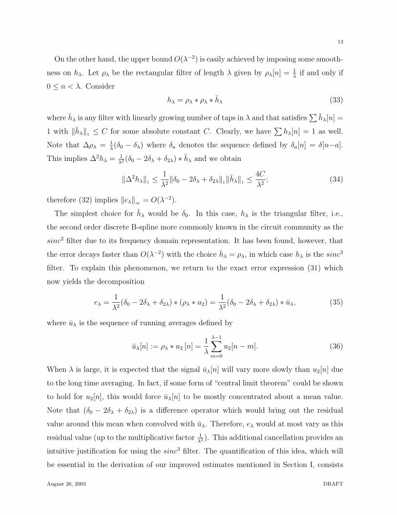
On the other hand, the upper bound O(λ−2) is easily achieved by imposing some smooth-

ness on hλ. Let ρλ be the rectangular filter of length λ given by ρλ[n] = 1λ

if and only if

0 ≤ n < λ. Consider

hλ = ρλ ∗ ρλ ∗ hλ (33)

where hλ is any filter with linearly growing number of taps in λ and that satisfies∑

hλ[n] =

1 with ‖hλ‖1 ≤ C for some absolute constant C. Clearly, we have∑

hλ[n] = 1 as well.

Note that ∆ρλ = 1λ(δ0 − δλ) where δa denotes the sequence defined by δa[n] = δ[n−a].

This implies ∆2hλ = 1λ2 (δ0 − 2δλ + δ2λ) ∗ hλ and we obtain

‖∆2hλ‖1 ≤1

λ2‖δ0 − 2δλ + δ2λ‖1‖hλ‖1 ≤

4C

λ2; (34)

therefore (32) implies ‖eλ‖∞ = O(λ−2).

The simplest choice for hλ would be δ0. In this case, hλ is the triangular filter, i.e.,

the second order discrete B-spline more commonly known in the circuit community as the

sinc2 filter due to its frequency domain representation. It has been found, however, that

the error decays faster than O(λ−2) with the choice hλ = ρλ, in which case hλ is the sinc3

filter. To explain this phenomenon, we return to the exact error expression (31) which

now yields the decomposition

eλ =1

λ2(δ0 − 2δλ + δ2λ) ∗ (ρλ ∗ u2) =

1

λ2(δ0 − 2δλ + δ2λ) ∗ uλ, (35)

where uλ is the sequence of running averages defined by

uλ[n] := ρλ ∗ u2 [n] =1

λ

λ−1∑m=0

u2[n−m]. (36)

When λ is large, it is expected that the signal uλ[n] will vary more slowly than u2[n] due

to the long time averaging. In fact, if some form of “central limit theorem” could be shown

to hold for u2[n], this would force uλ[n] to be mostly concentrated about a mean value.

Note that (δ0 − 2δλ + δ2λ) is a difference operator which would bring out the residual

value around this mean when convolved with uλ. Therefore, eλ would at most vary as this

residual value (up to the multiplicative factor 1λ2 ). This additional cancellation provides an

intuitive justification for using the sinc3 filter. The quantification of this idea, which will

be essential in the derivation of our improved estimates mentioned in Section I, consists


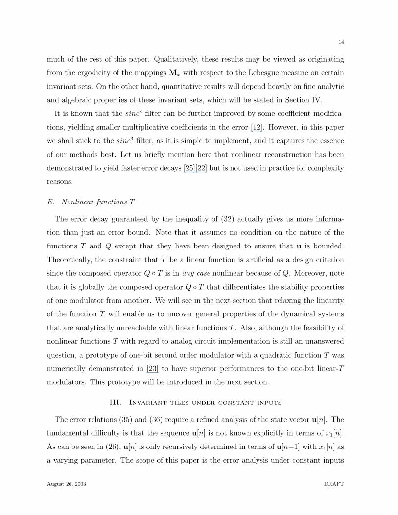
14

much of the rest of this paper. Qualitatively, these results may be viewed as originating

from the ergodicity of the mappings Mx with respect to the Lebesgue measure on certain

invariant sets. On the other hand, quantitative results will depend heavily on fine analytic

and algebraic properties of these invariant sets, which will be stated in Section IV.

It is known that the sinc3 filter can be further improved by some coefficient modifica-

tions, yielding smaller multiplicative coefficients in the error [12]. However, in this paper

we shall stick to the sinc3 filter, as it is simple to implement, and it captures the essence

of our methods best. Let us briefly mention here that nonlinear reconstruction has been

demonstrated to yield faster error decays [25][22] but is not used in practice for complexity

reasons.

E. Nonlinear functions T

The error decay guaranteed by the inequality of (32) actually gives us more informa-

tion than just an error bound. Note that it assumes no condition on the nature of the

functions T and Q except that they have been designed to ensure that u is bounded.

Theoretically, the constraint that T be a linear function is artificial as a design criterion

since the composed operator Q T is in any case nonlinear because of Q. Moreover, note

that it is globally the composed operator Q T that differentiates the stability properties

of one modulator from another. We will see in the next section that relaxing the linearity

of the function T will enable us to uncover general properties of the dynamical systems

that are analytically unreachable with linear functions T . Also, although the feasibility of

nonlinear functions T with regard to analog circuit implementation is still an unanswered

question, a prototype of one-bit second order modulator with a quadratic function T was

numerically demonstrated in [23] to have superior performances to the one-bit linear-T

modulators. This prototype will be introduced in the next section.

III. Invariant tiles under constant inputs

The error relations (35) and (36) require a refined analysis of the state vector u[n]. The

fundamental difficulty is that the sequence u[n] is not known explicitly in terms of x1[n].

As can be seen in (26), u[n] is only recursively determined in terms of u[n−1] with x1[n] as

a varying parameter. The scope of this paper is the error analysis under constant inputs


https://www.researchgate.net/publication/3325820_MSE_behavior_and_centroid_function_of_mth-order_asymptotic_SD_modulators?el=1_x_8&enrichId=rgreq-4276f12f34a15f58a8032eece18022b7-XXX&enrichSource=Y292ZXJQYWdlOzMwODUwMjU7QVM6MTIyMTg5NjkzMDY3MjY2QDE0MDYxNDM3MDE5NzM=

https://www.researchgate.net/publication/3316049_Vector_quantization_analysis_of_SD_modulation?el=1_x_8&enrichId=rgreq-4276f12f34a15f58a8032eece18022b7-XXX&enrichSource=Y292ZXJQYWdlOzMwODUwMjU7QVM6MTIyMTg5NjkzMDY3MjY2QDE0MDYxNDM3MDE5NzM=

https://www.researchgate.net/publication/3315219_Deterministic_Analysis_of_Oversampled_AD_Conversion_and_Decoding_Improvement_Based_on_Consistent_Estimates?el=1_x_8&enrichId=rgreq-4276f12f34a15f58a8032eece18022b7-XXX&enrichSource=Y292ZXJQYWdlOzMwODUwMjU7QVM6MTIyMTg5NjkzMDY3MjY2QDE0MDYxNDM3MDE5NzM=

https://www.researchgate.net/publication/3157459_Double-Loop_Sigma-Delta_Modulation_with_dc_Input?el=1_x_8&enrichId=rgreq-4276f12f34a15f58a8032eece18022b7-XXX&enrichSource=Y292ZXJQYWdlOzMwODUwMjU7QVM6MTIyMTg5NjkzMDY3MjY2QDE0MDYxNDM3MDE5NzM=

15

x1[n] = x, ∀n. In this situation, u[n] recursively depends on u[n−1] through the fixed

mapping Mx, i.e.,

u[n] = Mx(u[n−1]). (37)

The key to the analysis lies in the study of the map Mx.

A. Experimental observation of tiling

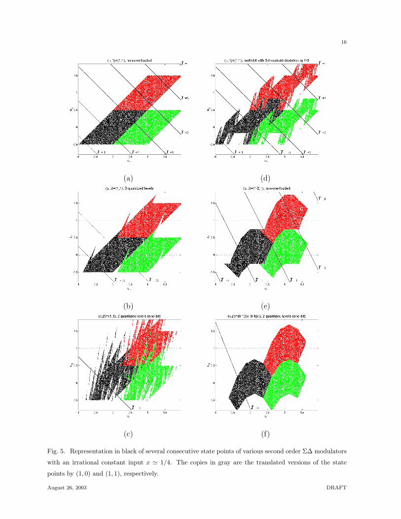
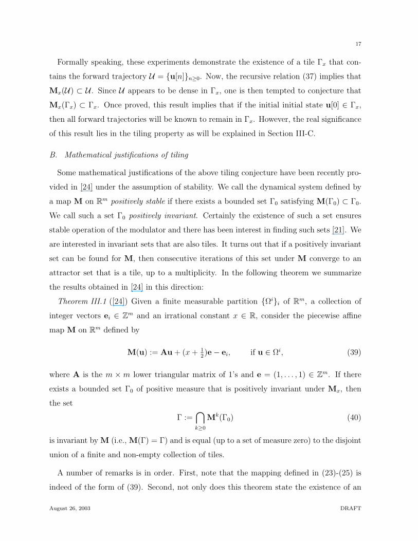
We start with the description of a particular experiment that lead to the discovery of a

remarkable property of the maps Mx. For various second order Σ∆ modulators, we plot

in black in Figure 5 several consecutive iterates u[n] of a fixed initial condition u[0] under

the map Mx, where x is a fixed constant input. In these plots, x is chosen to be irrational;

we will return to this issue later. For each modulator, one can observe in this plot that

the state points remain in (and fill out) a certain deterministic set Γ := Γx. However,

there is more to this set in that in every case its integer (Z2) translations appear to tile

the plane. We highlight this fact in the figure by representing the translates of the points

u[n] by (1, 0) and (1, 1) in two gray tones, respectively. Formally, we say that a set Γ is

a tile when for each point v ∈ R2, there is a unique point v′ ∈ Γ such that v − v′ ∈ Z2.

This is equivalent to the fact that the family Γ + kk∈Z2 forms a partition of R2.

Since the initial observation of this phenomenon [9], it has been systematically confirmed

on any stable second order modulator employing a quantizer with uniformly spaced output

levels as assumed in this paper. In the cases of Figures 5(a) through 5(d), the standard

linear rule T (u1, u2, x) = u1 +u2 +x is used with different versions of the quantizer. Figure

5(a) is the case of the non-overloaded ideal quantizer (infinite quantizer). In Figure 5(b)

we use the 3-level quantizer introduced in [26] which employs −1, 0, 1 as the output levels

and 12,−1

2as the threshold values. Figure 5(c) is the standard one-bit quantizer case. In

Figure 5(d) we use an infinite quantizer whose threshold at 0 has been deviated by +13.

Figure 5(e) shows the case of a different linear rule T (u1, u2, x) = u1 + 12u2 + x with the

regular infinite quantizer. Finally, Figure 5(f) shows the case of the following “semi-linear”

rule introduced in [23]:

T (u1, u2, x) = (9− 6|x|)u1 + (6− 12|x|)u2 + (10− 4|x|)x. (38)


16

(a) (d)

(b) (e)

(c) (f)

Fig. 5. Representation in black of several consecutive state points of various second order Σ∆ modulators

with an irrational constant input x ' 1/4. The copies in gray are the translated versions of the state

points by (1, 0) and (1, 1), respectively.


17

Formally speaking, these experiments demonstrate the existence of a tile Γx that con-

tains the forward trajectory U = u[n]n≥0. Now, the recursive relation (37) implies that

Mx(U) ⊂ U . Since U appears to be dense in Γx, one is then tempted to conjecture that

Mx(Γx) ⊂ Γx. Once proved, this result implies that if the initial initial state u[0] ∈ Γx,

then all forward trajectories will be known to remain in Γx. However, the real significance

of this result lies in the tiling property as will be explained in Section III-C.

B. Mathematical justifications of tiling

Some mathematical justifications of the above tiling conjecture have been recently pro-

vided in [24] under the assumption of stability. We call the dynamical system defined by

a map M on Rm positively stable if there exists a bounded set Γ0 satisfying M(Γ0) ⊂ Γ0.

We call such a set Γ0 positively invariant. Certainly the existence of such a set ensures

stable operation of the modulator and there has been interest in finding such sets [21]. We

are interested in invariant sets that are also tiles. It turns out that if a positively invariant

set can be found for M, then consecutive iterations of this set under M converge to an

attractor set that is a tile, up to a multiplicity. In the following theorem we summarize

the results obtained in [24] in this direction:

Theorem III.1 ([24]) Given a finite measurable partition Ωii of Rm, a collection of

integer vectors ei ∈ Zm and an irrational constant x ∈ R, consider the piecewise affine

map M on Rm defined by

M(u) := Au + (x + 12)e− ei, if u ∈ Ωi, (39)

where A is the m × m lower triangular matrix of 1’s and e = (1, . . . , 1) ∈ Zm. If there

exists a bounded set Γ0 of positive measure that is positively invariant under Mx, then

the set

Γ :=⋂k≥0

Mk(Γ0) (40)

is invariant by M (i.e., M(Γ) = Γ) and is equal (up to a set of measure zero) to the disjoint

union of a finite and non-empty collection of tiles.

A number of remarks is in order. First, note that the mapping defined in (23)-(25) is

indeed of the form of (39). Second, not only does this theorem state the existence of an


https://www.researchgate.net/publication/3322918_An_algorithm_for_computing_convex_positively_invariant_sets_for_Delta-Sigma_modulators?el=1_x_8&enrichId=rgreq-4276f12f34a15f58a8032eece18022b7-XXX&enrichSource=Y292ZXJQYWdlOzMwODUwMjU7QVM6MTIyMTg5NjkzMDY3MjY2QDE0MDYxNDM3MDE5NzM=




18

invariant set Γ, but (40) shows that Γ is an attractor of M within the region of stability Γ0.

Next, note that this theorem is valid in any dimensions m and under general conditions

on the partition Ωii as well as the integer translations ei, as long as the overall map M

is positively stable. However, under these general assumptions, the conclusion is only that

Γ is composed of one or more tiles, all up to a set of measure zero. Indeed, an example

given in [24] shows that a map of the type (25) may yield an invariant set composed of two

tiles. Let us note that this example required the use of a particular nonlinear thresholding

function T . The exact conditions on T to yield a single tile are not currently known. From

our experience (including, for example, the experiments of Figure 5), we believe that all

stable Σ∆ modulators using a linear thresholding function T yield a single invariant tile,

at least at the second order and including the case of rational input constants x. However,

care must be taken in the definition of the invariant set Γ when x is a rational number;

the statement is on the existence of a tile Γ that is invariant under M and it may not

necessarily be the case that Γ can be found as an attractor as in (40) or the closure of any

trajectory. It remains a general conjecture that linear thresholding functions enjoy these

properties. In Section IV, we will give the proof of these properties on three particular

configurations of second order Σ∆ modulation. But before performing this analysis, we

would like to show why the single tile case is of crucial importance.

C. The single invariant tile case and its fundamental consequence

From now on we only consider Σ∆ modulators for which the invariant set Γx is a single

tile for each x. We shall see in this case that it is possible to find an explicit expression

for u[n] in terms of n and Γx. To keep the discussion simple we shall restrict ourselves to

second order modulators; the generalization to higher order modulators is routine.

We first introduce some notation. Let Γ be an arbitrary tile in R2. By definition, the

collection of sets Γ + kk∈Z2 form a partition of R2. This implies that for each u ∈ R2,

there exists a unique point in Γ, denoted 〈u〉Γ, such that

〈u〉Γ− u ∈ Z2. (41)

In other words, u 7→ 〈u〉Γ

is the unique map from R2 to Γ that satisfies

∀u ∈ Γ, 〈u〉Γ

= u, (42)



19

−1 −0.5 0 0.5 1 1.5 2 2.5 3−1

−0.5

0

0.5

1

1.5

2

u1

u 2

u[n+1]

v[n+1]

u[n]

v[n] u[n−1]

v[n−1]

Γ

(a)

−1 −0.5 0 0.5 1 1.5 2−1

−0.5

0

0.5

1

1.5

2

u1

u 2

Γ S(0,0)

S(−1,0)

S(−1,−1)

S(0,−1)

u

< u>

< u>Γ

(b)

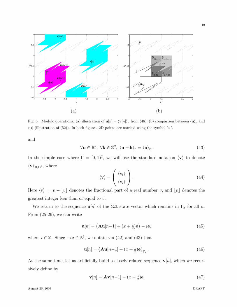
Fig. 6. Modulo operations: (a) illustration of u[n] = 〈v[n]〉Γ

from (48); (b) comparison between 〈u〉Γ

and

〈u〉 (illustration of (52)). In both figures, 2D points are marked using the symbol ’×’.

and

∀u ∈ R2, ∀k ∈ Z2, 〈u + k〉Γ

= 〈u〉Γ. (43)

In the simple case where Γ = [0, 1)2, we will use the standard notation 〈v〉 to denote

〈v〉[0,1)2 , where

〈v〉 =

〈v1〉

〈v2〉

. (44)

Here 〈v〉 := v − bvc denotes the fractional part of a real number v, and bvc denotes the

greatest integer less than or equal to v.

We return to the sequence u[n] of the Σ∆ state vector which remains in Γx for all n.

From (25-26), we can write

u[n] =(Au[n−1] + (x + 1

2)e)− ie, (45)

where i ∈ Z. Since −ie ∈ Z2, we obtain via (42) and (43) that

u[n] =⟨Au[n−1] + (x + 1

2)e⟩

Γx. (46)

At the same time, let us artificially build a closely related sequence v[n], which we recur-

sively define by

v[n] = Av[n−1] + (x + 12)e (47)


20

with the initial state v[0] = u[0]. We have the following property:

Proposition III.2: For all n, we have

u[n] = 〈v[n]〉Γx . (48)

Proof: Since 〈v〉Γx − v ∈ Z2 and A is a matrix with all integer coefficients, we have

A〈v〉Γx −Av = A(〈v〉Γx − v) ∈ Z2. It follows from (43) that

〈A 〈v〉Γx + w〉Γx = 〈Av + w〉Γx (49)

for any w ∈ R2. The proposition is then proved by induction. For n = 0, we have

u[0] = 〈u[0]〉Γx = 〈v[0]〉Γx . Suppose (48) holds for k = n − 1, i.e. u[n−1] = 〈v[n−1]〉Γx .

Then, by successively applying (46), (49) and (47), we obtain

u[n] =⟨A〈v[n−1]〉Γx + (x + 1

2)e⟩

Γx

=⟨Av[n−1] + (x + 1

2)e⟩

Γx

= 〈v[n]〉Γx.

The power of this result lies in the fact that there is an explicit functional expression

for v[n] which can be obtained by simply iterating (47) forwards and backwards:

∀n ∈ Z, v[n] =

v1[n]

v2[n]

=

u1[0] + n(x + 12)

nu1[0] + u2[0] + 12n(n + 1)(x + 1

2)

. (50)

Thus, under the assumption that the tile Γx is known, the combination of (48) and (50)

provides an explicit expression of u[n] in terms of n.

We define u[n] for n < 0 by (48). It follows from the invariance of Γx under Mx that

this definition is consistent with (37) for all n ∈ Z.

Figure 6(a) gives a graphical example of explicit determination of the sequence u[n]

from the knowledge of the tile, via the preliminary calculation of the sequence v[n] from

(50).

D. Further developments on the single tile case

A remaining major difficulty of analysis is that the expression (48) for u[n] depends on

the knowledge of the invariant set Γx. Not only that this set can be complex as in some of


21

the examples in Figure 5, but also explicit expressions are, in general, not easily obtainable.

Nevertheless, an analysis of u[n] is still possible, thanks to a particular decomposition of

〈·〉Γx into simpler components. This is based on the following lemma:

Lemma III.3: Let Γ and Γ′ be two sets that tile the plane with Z2 translations. For

each k ∈ Z2, let us define the set Πk := u : 〈u〉Γ∈ Γ′ − k . Then

(i) the family Πkk∈Z2 forms a partition of R2,

(ii) 〈u〉Γ′− 〈u〉

Γ= k when u ∈ Πk.

Proof: Since Γ′ tiles the plane with Z2 translations, for any u ∈ R2, there exists a

unique k ∈ Z2 such that 〈u〉Γ∈ Γ′ − k. This proves part (i). Now, consider any given

k ∈ Z2 and any u ∈ Πk. By definition, 〈u〉Γ∈ Γ′ − k, and we have 〈u〉

Γ+ k ∈ Γ′. Since

〈u〉Γ

+ k differs from u by an element in Z2, and itself lies in Γ′, it must indeed be equal

to 〈u〉Γ′

, i.e., 〈u〉Γ′− 〈u〉

Γ= k.

Lemma III.3 actually leads to the following explicit relation

〈u〉Γ′ = 〈u〉Γ +∑k∈Z2

χΠk

(u) k,

where χA

stands for the characteristic function of the set A. Note that 〈u〉Γ

always belongs

to Γ. Hence u ∈ Πk if and only if 〈u〉Γ∈ Γk := Γ ∩ (Γ′ − k). We can then also write

〈u〉Γ′ = 〈u〉Γ +∑k∈Z2

χΓk

(〈u〉Γ) k. (51)

Of particular interest will be the case where Γ′ = Γx and Γ = [0, 1)2. This yields

〈u〉Γx = 〈u〉+∑k∈Z2

χSk

(〈u〉) k. (52)

where Sk := [0, 1)2∩(Γx−k). This is the decomposition of the function 〈·〉Γx as mentioned

earlier.

Another useful property is the following:

Proposition III.4: Let Γ and Γ′ be two (Lebesgue) measurable sets that tile the plane

with the Z2 lattice. Then 〈·〉Γ as a mapping from Γ′ to Γ is a (Lebesgue) measure preserving

bijection whose inverse is given by 〈·〉Γ′ . If F : R2 → R is any Z2-periodic locally integrable

function, then ∫Γ

F (u)du =

∫Γ′

F (u)du. (53)


22

Proof: Bijectivity is clear. On the other hand, if u ∈ Γ′, then 〈〈u〉Γ〉Γ′ = u, since each

of these mappings shifts its argument by an element of Z2, and the resulting point lies in

Γ′. Hence 〈·〉Γ′ inverts 〈·〉Γ. Now, for any k ∈ Z2, let us define Γk := Γ∩(Γ′−k) and Γ′k :=

Γ′ ∩ (Γ − k). It follows easily from the tiling assumption that the families Γkk∈Z2 and

Γ′kk∈Z2 form partitions of Γ and Γ′, respectively. It is also easy to see that Γ′k = Γ−k−k.

Now, for a measurable set A ⊂ Γ, (51) implies that 〈A〉Γ′

=⋃

k∈Z2 ((A ∩ Γk) + k). This is

a disjoint union, and it follows that |〈A〉Γ′| =∑

k∈Z2 |A∩ Γk + k| =∑

k∈Z2 |A∩ Γk| = |A|.

Hence 〈·〉Γ preserves measure.

Since F is Z2-periodic, we have F (u) = F (〈u〉Γ′). Using this and the measure preserving

property of 〈·〉Γ′ , we get∫Γ

F (u)du =

∫Γ

F (〈u〉Γ′)du =

∫Γ′

F (v)dv. (54)

We conclude this section with a word is on the dynamics of Mx on the invariant set Γx.

Consider the mapping 〈Mx〉 : [0, 1)2 → [0, 1)2 naturally defined by 〈Mx〉(u) = 〈Mx(u)〉.

It can be easily checked that the mappings Mx|Γxand 〈Mx〉 are related to each other via

Mx|Γx= 〈·〉Γx 〈Mx〉〈·〉.

It is well known that when x is irrational, 〈Mx〉 is ergodic with respect to the Lebesgue

measure (see e.g. [20]). Since both 〈·〉Γx : [0, 1)2 → Γx and 〈·〉 : Γx → [0, 1)2 are measure

preserving, it follows that Mx (and also M−1x ) is ergodic on Γx with respect to the Lebesgue

measure as well. This is the ergodicity property that was mentioned at the end of Section

II-D.

IV. Thorough study of three particular configurations

The purpose of this section is three-fold. First, we would like to give some concrete

examples of invariant tiles Γx in some practical configurations. Recall from the previous

section that a general criterion regarding when the invariant sets reduce to single tiles is not

available yet and also that our signal analysis machinery is dependent on this condition.

Second, we will see in these examples that tiling phenomenon is not restricted to irrational

inputs but that it applies to rational inputs as well. Third, we would like to extract some


https://www.researchgate.net/publication/266013032_Topics_in_Ergodic_Theory?el=1_x_8&enrichId=rgreq-4276f12f34a15f58a8032eece18022b7-XXX&enrichSource=Y292ZXJQYWdlOzMwODUwMjU7QVM6MTIyMTg5NjkzMDY3MjY2QDE0MDYxNDM3MDE5NzM=

23

common analytical features of these invariant sets which will later be crucial in the error

analysis of Section V.

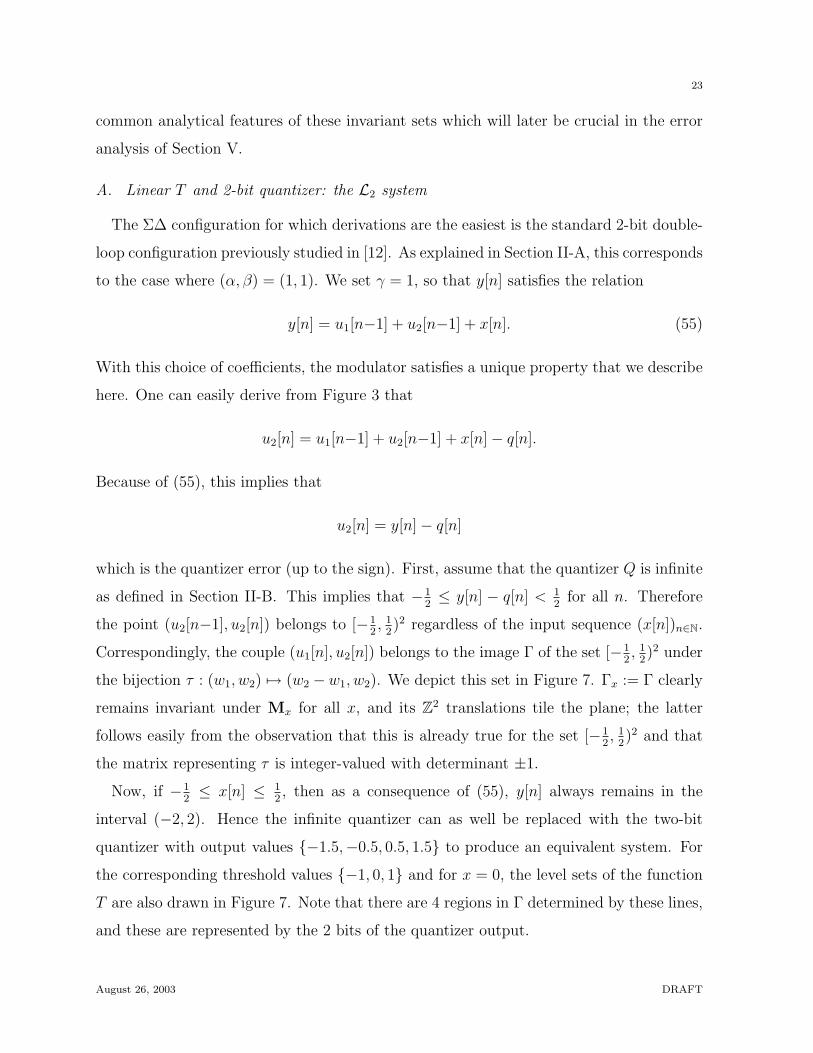
A. Linear T and 2-bit quantizer: the L2 system

The Σ∆ configuration for which derivations are the easiest is the standard 2-bit double-

loop configuration previously studied in [12]. As explained in Section II-A, this corresponds

to the case where (α, β) = (1, 1). We set γ = 1, so that y[n] satisfies the relation

y[n] = u1[n−1] + u2[n−1] + x[n]. (55)

With this choice of coefficients, the modulator satisfies a unique property that we describe

here. One can easily derive from Figure 3 that

u2[n] = u1[n−1] + u2[n−1] + x[n]− q[n].

Because of (55), this implies that

u2[n] = y[n]− q[n]

which is the quantizer error (up to the sign). First, assume that the quantizer Q is infinite

as defined in Section II-B. This implies that −12≤ y[n] − q[n] < 1

2for all n. Therefore

the point (u2[n−1], u2[n]) belongs to [−12, 1

2)2 regardless of the input sequence (x[n])n∈N.

Correspondingly, the couple (u1[n], u2[n]) belongs to the image Γ of the set [−12, 1

2)2 under

the bijection τ : (w1, w2) 7→ (w2 −w1, w2). We depict this set in Figure 7. Γx := Γ clearly

remains invariant under Mx for all x, and its Z2 translations tile the plane; the latter

follows easily from the observation that this is already true for the set [−12, 1

2)2 and that

the matrix representing τ is integer-valued with determinant ±1.

Now, if −12≤ x[n] ≤ 1

2, then as a consequence of (55), y[n] always remains in the

interval (−2, 2). Hence the infinite quantizer can as well be replaced with the two-bit

quantizer with output values −1.5,−0.5, 0.5, 1.5 to produce an equivalent system. For

the corresponding threshold values −1, 0, 1 and for x = 0, the level sets of the function

T are also drawn in Figure 7. Note that there are 4 regions in Γ determined by these lines,

and these are represented by the 2 bits of the quantizer output.


24

T=1

T=0

T=−1

AB

C D

Γ

u

u

1

2

Fig. 7. The invariant set for the dynamical systems Mx considered in Section IV-A. The level sets of

T (·) are drawn for x = 0.

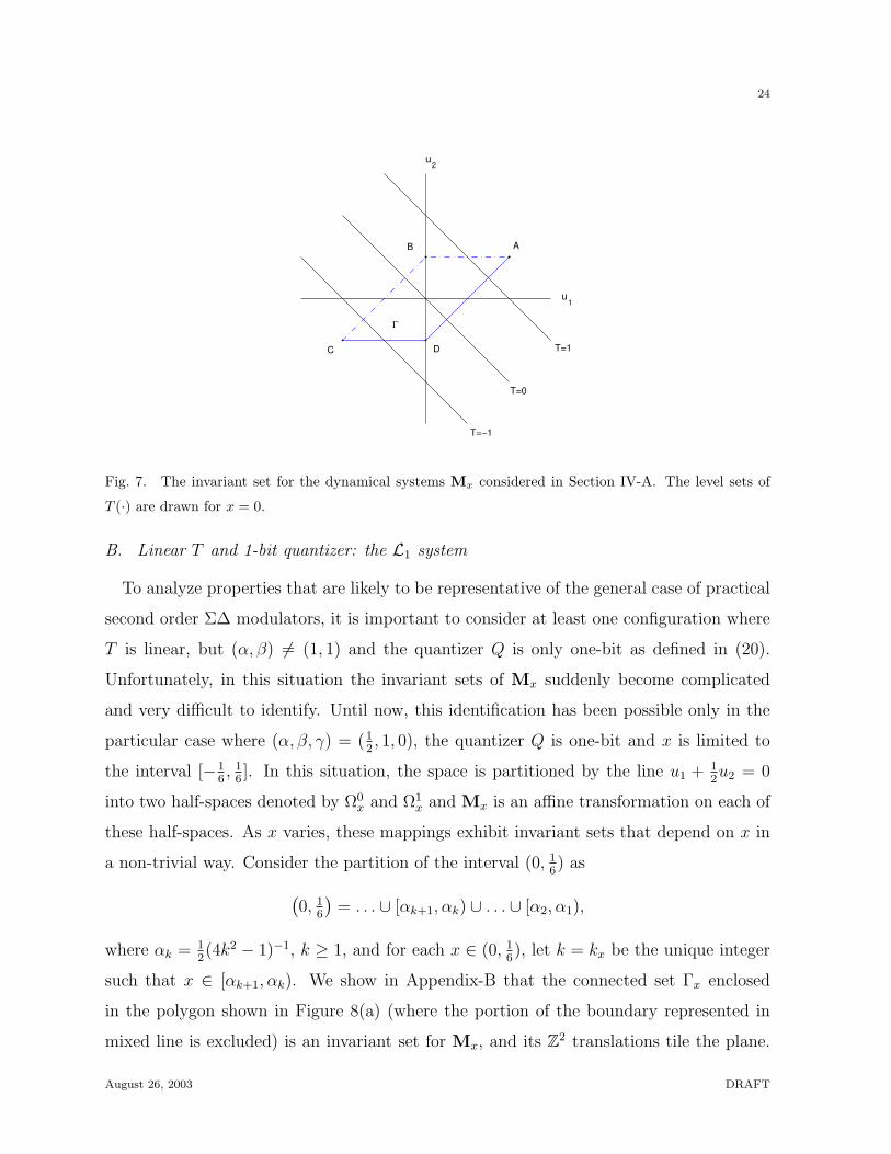
B. Linear T and 1-bit quantizer: the L1 system

To analyze properties that are likely to be representative of the general case of practical

second order Σ∆ modulators, it is important to consider at least one configuration where

T is linear, but (α, β) 6= (1, 1) and the quantizer Q is only one-bit as defined in (20).

Unfortunately, in this situation the invariant sets of Mx suddenly become complicated

and very difficult to identify. Until now, this identification has been possible only in the

particular case where (α, β, γ) = (12, 1, 0), the quantizer Q is one-bit and x is limited to

the interval [−16, 1

6]. In this situation, the space is partitioned by the line u1 + 1

2u2 = 0

into two half-spaces denoted by Ω0x and Ω1

x and Mx is an affine transformation on each of

these half-spaces. As x varies, these mappings exhibit invariant sets that depend on x in

a non-trivial way. Consider the partition of the interval (0, 16) as(

0, 16

)= . . . ∪ [αk+1, αk) ∪ . . . ∪ [α2, α1),

where αk = 12(4k2 − 1)−1, k ≥ 1, and for each x ∈ (0, 1

6), let k = kx be the unique integer

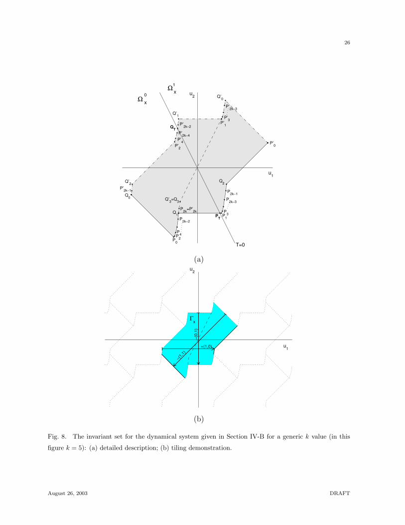
such that x ∈ [αk+1, αk). We show in Appendix-B that the connected set Γx enclosed

in the polygon shown in Figure 8(a) (where the portion of the boundary represented in

mixed line is excluded) is an invariant set for Mx, and its Z2 translations tile the plane.


25

The exact definition of the vertices of Γx is given in Appendix-B, Table II. Note that the

total number of vertices is equal to 4k + 6, which increases indefinitely as x approaches 0.

We add that Γ0 and Γ 16

are obtained via the limits of Px, as x → 0 and x → 16. Together

with the symmetry Γx = −Γ−x, which is a mere consequence of the relation

T (−u,−x) = −T (u, x), (56)

we obtain the parameterization of all Γx in the range [−16, 1

6].

We also note that the polygonal boundary of Γx has bounded perimeter for all x ∈

[−16, 1

6].

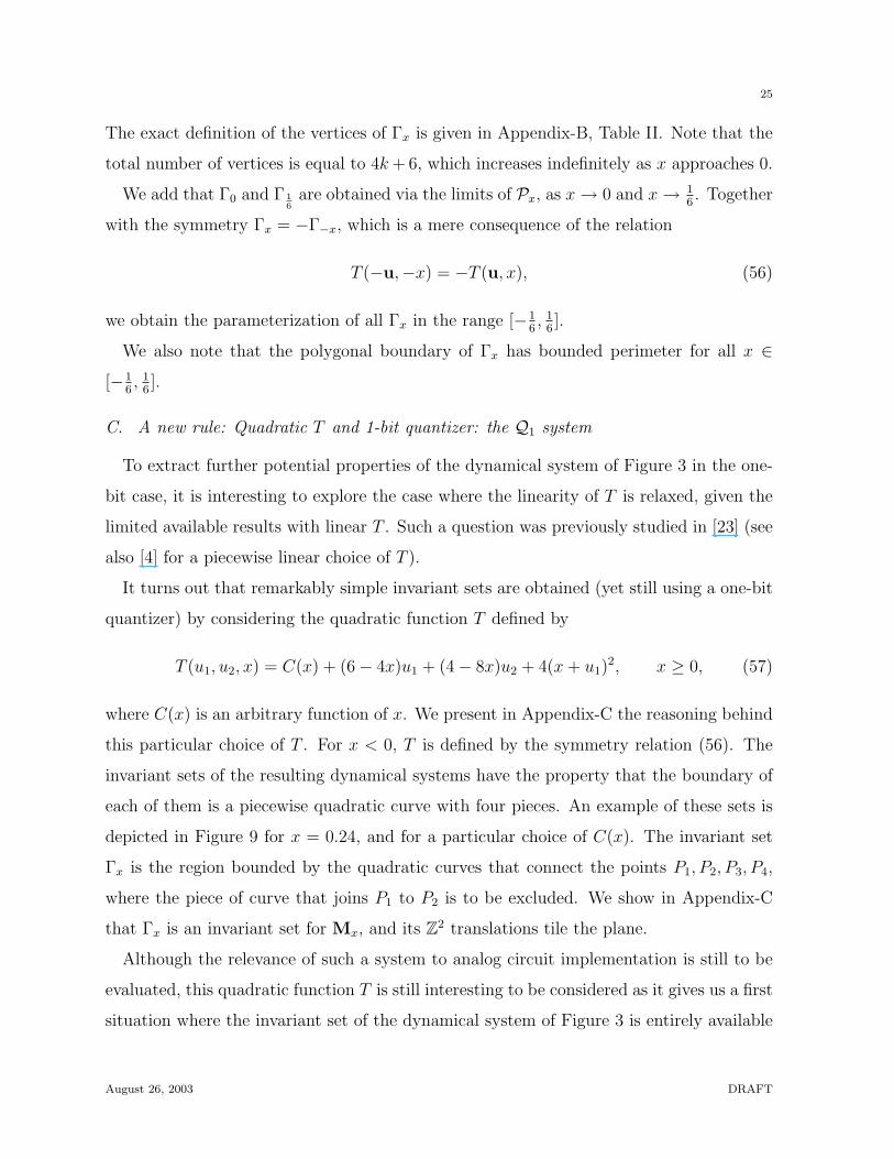
C. A new rule: Quadratic T and 1-bit quantizer: the Q1 system

To extract further potential properties of the dynamical system of Figure 3 in the one-

bit case, it is interesting to explore the case where the linearity of T is relaxed, given the

limited available results with linear T . Such a question was previously studied in [23] (see

also [4] for a piecewise linear choice of T ).

It turns out that remarkably simple invariant sets are obtained (yet still using a one-bit

quantizer) by considering the quadratic function T defined by

T (u1, u2, x) = C(x) + (6− 4x)u1 + (4− 8x)u2 + 4(x + u1)2, x ≥ 0, (57)

where C(x) is an arbitrary function of x. We present in Appendix-C the reasoning behind

this particular choice of T . For x < 0, T is defined by the symmetry relation (56). The

invariant sets of the resulting dynamical systems have the property that the boundary of

each of them is a piecewise quadratic curve with four pieces. An example of these sets is

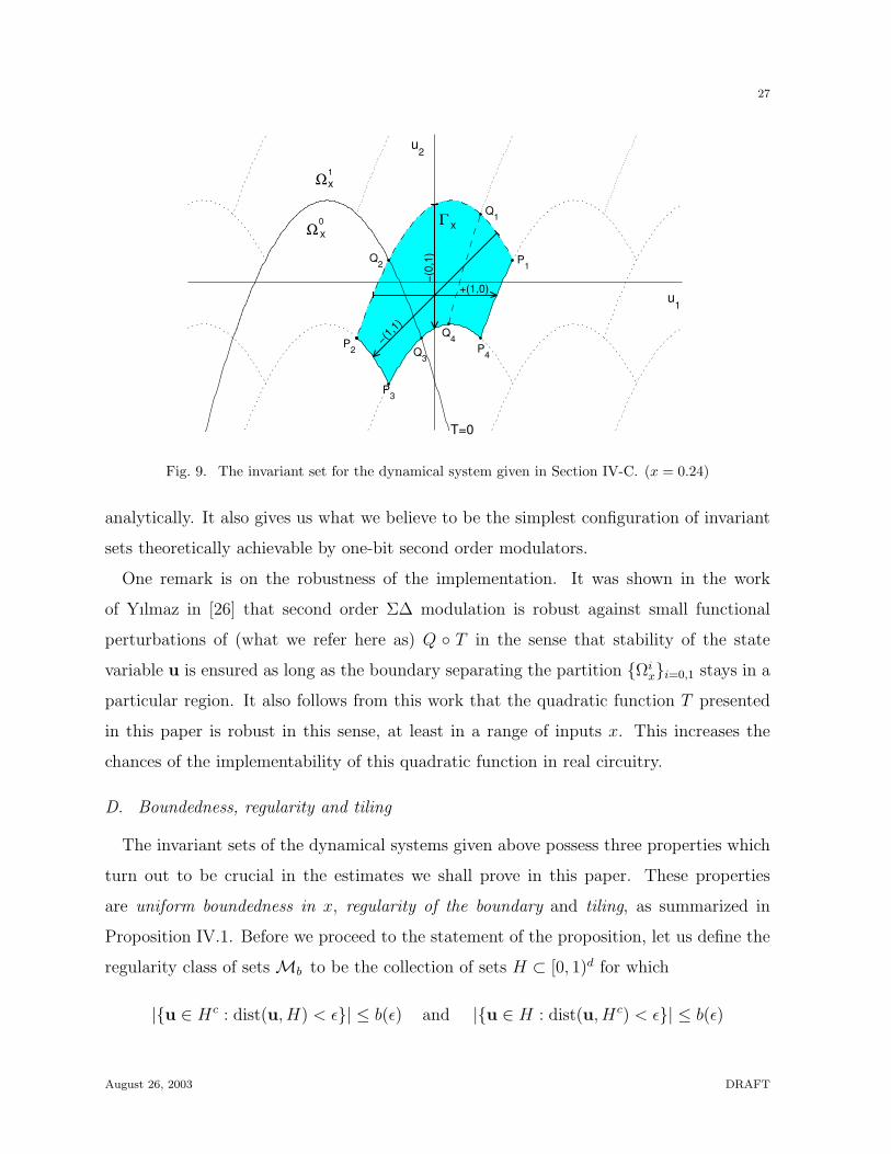
depicted in Figure 9 for x = 0.24, and for a particular choice of C(x). The invariant set

Γx is the region bounded by the quadratic curves that connect the points P1, P2, P3, P4,

where the piece of curve that joins P1 to P2 is to be excluded. We show in Appendix-C

that Γx is an invariant set for Mx, and its Z2 translations tile the plane.

Although the relevance of such a system to analog circuit implementation is still to be

evaluated, this quadratic function T is still interesting to be considered as it gives us a first

situation where the invariant set of the dynamical system of Figure 3 is entirely available




26

u2

u1

P’3

P0

P2

P2k−2

P2k

=P’2kQ

1

Q’3=Q

3

P4

P’2

P’4

P’2k−2

Q’1

QT

PT P1

P3

P2k−1

Q2

P’0

Q0

P’2k−1

Q’2

P’1

Q’0

T=0

Ω Ω

x

x 0

1

P’2k−3

P2k−3

P’2k−4

(a)

−(1,1

)+(1,0)

−(0,

1)

u1

u2

x Γ

(b)

Fig. 8. The invariant set for the dynamical system given in Section IV-B for a generic k value (in this

figure k = 5): (a) detailed description; (b) tiling demonstration.


27

−(1,1

)

+(1,0)

−(0,

1)

u1

u2

T=0

Q4

Q3

P3

P2

Q2

Q1

P1

P4

Γ x Ω 0 x

Ω 1 x

Fig. 9. The invariant set for the dynamical system given in Section IV-C. (x = 0.24)

analytically. It also gives us what we believe to be the simplest configuration of invariant

sets theoretically achievable by one-bit second order modulators.

One remark is on the robustness of the implementation. It was shown in the work

of Yılmaz in [26] that second order Σ∆ modulation is robust against small functional

perturbations of (what we refer here as) Q T in the sense that stability of the state

variable u is ensured as long as the boundary separating the partition Ωixi=0,1 stays in a

particular region. It also follows from this work that the quadratic function T presented

in this paper is robust in this sense, at least in a range of inputs x. This increases the

chances of the implementability of this quadratic function in real circuitry.

D. Boundedness, regularity and tiling

The invariant sets of the dynamical systems given above possess three properties which

turn out to be crucial in the estimates we shall prove in this paper. These properties

are uniform boundedness in x, regularity of the boundary and tiling, as summarized in

Proposition IV.1. Before we proceed to the statement of the proposition, let us define the

regularity class of sets Mb to be the collection of sets H ⊂ [0, 1)d for which

|u ∈ Hc : dist(u, H) < ε| ≤ b(ε) and |u ∈ H : dist(u, Hc) < ε| ≤ b(ε)


28

for every ε > 0, where b : (0,∞) → (0,∞) is a monotonically increasing function such

that limε→0+ b(ε) = 0. Here |A| denotes the (Lebesgue) measure of the set A, and Ac

denotes the complement of A. Every Jordan measurable set (i.e. a set whose boundary

has Lebesgue measure zero) belongs to such a class Mb for some b.

Proposition IV.1: For each of the one-parameter family of dynamical systems D =

(Mx, x ∈ [−12, 1

2]) given in Sections IV-A, IV-B, and IV-C, there exists a subinterval

I = I(D) of [−12, 1

2] such that for each x ∈ I, the map Mx possesses an invariant set Γx

with the following properties:

1. Uniform boundedness in x: There exists a positive constant M0 such that

supx∈I

supu∈Γx

|u| ≤ M0.

2. Regularity of the boundary: There exists a positive constant C0 such that Γx ∈Mb for

all x ∈ I, where b(ε) = C0ε.

3. Tiling: For each x ∈ I, the set Γx is a tile congruent to [0, 1)2 modulo translations by

vectors in Z2. I.e., the translates of Γx by the integer lattice tile the plane:

Γx + Z2 = R2, and (Γx + k) ∩ Γx = ∅ if k ∈ Z2\0.

We say that Γx is a tiling invariant set, or equivalently an invariant tile.

The proof of this proposition is given in Appendix-D.

V. The Main Theorem

We shall continue to use the notation L2, L1, and Q1 to denote the one-parameter

dynamical systems D = (Mx, x ∈ [−12, 1

2]) for the 2-bit linear, 1-bit linear, and the 1-bit

quadratic schemes given in Sections IV-A, IV-B, and IV-C, respectively. For each of these

second order Σ∆ schemes, we assume that for each x ∈ I(D), the initial condition u[0] is

chosen from the invariant set Γx of the associated dynamical system Mx, and the sequence

u[n] is defined for all n ∈ Z as described in Section III-C. Recall that the subscript x in

eλ,x[n] denotes the dependence of the error eλ[n] = hλ ∗ (x1[n] − q[n]) on the value x of

the constant input signal x1[n], and hλ is the sinc3 filter defined in Section II-D. For each

family D ∈ L2,L1,Q1, we set, as in Section I,

MSE(λ;D) = supn

∫I

|eλ,x[n]|2 dx, (58)


29

where I = I(D) is as defined in Proposition IV.1. The following theorem lists our improved

estimates for these second order schemes:

Theorem V.1: Let D be a second order Σ∆ modulation scheme that satisfies the prop-

erties listed in Proposition IV.1, in particular any of the schemes L2, L1 or Q1. Then the

following estimates hold:

(a) The mean square error defined by (58) satisfies

MSE(λ;D) ≤ Cλ−9/2 log2 λ (59)

for all λ > 0, where C = C(D) is a constant that depends only on the scheme D.

(b) For almost every x ∈ I, and all n ∈ Z,

|eλ,x[n]|2 ≤ Cλ−9/2 log4 λ (60)

for all λ > 0, where C = C(D, x, n) does not depend on λ, but otherwise may depend on

the scheme D, input x and the time point n.

(c) For D = L2, the same estimates in (a) and (b) hold with 9/2 replaced by 5.

Before we proceed onto the proof of the theorem, let us list some further qualitative

observations. Equation (35) states that

eλ,x[n] =1

λ2(uλ[n]− 2uλ[n−λ] + uλ[n−2λ]) . (61)

As a reminder from (36), uλ[n] is qualitatively the average of the discrete sequence u2[m]

over the time interval of (n − λ, n]. This expression immediately suggests that eλ,x[n] =

o(λ−2). To see this, denote by F2 the mapping that takes u = (u1, u2) to u2. When x is

irrational, for almost all u[0] and for all n, the Ergodic Theorem yields

limλ→∞

uλ[n] = limλ→∞

1

λ

λ−1∑j=0

F2(M−jx u[n]) =

∫Γx

F2(w) dw =

∫Γx

w2 dw1dw2. (62)

Now, it is a simple exercise to show that

uλ[n]− 2uλ[n−λ] + uλ[n−2λ] = 3(uλ[n]− 2u2λ[n] + u3λ[n]

); (63)


30

therefore (61) and (62) together imply that eλ,x[n] = o(λ−2). Note that this argument

does not provide us with any information about the improvement on the exponent of λ.

The proof of Theorem V.1 below will heavily use techniques from the theory of uniform

distribution. Appendix-A contains the definitions and the tools that we shall employ in

the proof.

Proof of Theorem V.1: Let us define a residual sequence rλ by

rλ[n] := uλ[n]−∫

Γx

w2 dw1dw2 =1

λ

∑n−λ<m≤n

F2(u[m])−∫

Γx

F2(w) dw. (64)

Since uλ[n] and rλ[n] differ by an absolute constant, we can replace uλ[n] in (63) by rλ[n].

When combined with (61), this yields

|eλ,x[n]| =3

λ2|rλ[n]− 2r2λ[n] + r3λ[n]|

≤ 3

λ2

(|rλ[n]|+ |2r2λ[n]|+ |r3λ[n]|

), (65)

and by Cauchy-Schwarz,

|eλ,x[n]|2 ≤ C

λ4

(|rλ[n]|2 + |r2λ[n]|2 + |r3λ[n]|2

); (66)

therefore it suffices, for each time point n, to estimate |rλ[n]| for general λ.

Let us first consider the rather simple case D = L2. Note that the invariant set Γx given

in Figure 7 is such that the ordinate of any point in Γx always lies in [−12, 1

2). Also, the

sequence v[n] defined in Section III-C satisfies u2[n]− v2[n] ∈ Z. Therefore

u2[n] = 〈v2[n]〉[− 1

2 , 12 )= 〈v2[n] + 1

2〉 − 1

2. (67)

Since in this case

∫Γx

w2dw1dw2 = 0, (64) becomes

rλ[n] =1

λ

∑n−λ<m≤n

(〈v2[m] + 1

2〉 − 1

2

)=

1

λ

∑n−λ<m≤n

〈v2[m] + 12〉 −

∫ 1

0

w dw. (68)

Let D(n−λ,n](〈v2〉) denote the discrepancy (Appendix-A) of the λ consecutive sequence

elements 〈v2[m]〉; n−λ < m ≤ n. Koksma’s inequality (Appendix-A) can be used to

bound |rλ[n]|:

|rλ[n]| ≤ D(n−λ,n](〈v2〉), (69)


31

where we have used the invariance of discrepancy under translations of the torus T = [0, 1)

in the equality D(n−λ,n](〈v2 + 12〉) = D(n−λ,n](〈v2〉). The estimate (69) therefore reduces the

problem for the case D = L2 to estimating the λ-term discrepancy of the sequence 〈v2〉.

The general case for D which includes D ∈ L1,Q1 is more difficult because it is no

longer possible to obtain an expression of u2[n] as simple as in (67). Initially, the expression

(64) suggests the need for some two-dimensional version of Koksma’s inequality, defined

on an arbitrary set (in our case Γx); however, the setup for the so-called Koksma-Hlawka

inequality [5, Theorem 1.14]) is the unit cube [0, 1)d. Using (48), the Z2-periodicity of

〈·〉Γx

, and Proposition III.4, we can transform the expression (64) into

rλ[n] =1

λ

∑n−λ<m≤n

F2

(⟨〈v[m]〉

⟩Γx

)−∫

[0,1)2F2

(〈w〉

Γx

)dw, (70)

and attempt to use the Koksma-Hlawka inequality for the sequence 〈v[m]〉 and the function

f = F2 〈·〉Γx. At first, this attempt also appears to be defeated because Koksma-Hlawka

inequality holds for functions that are of bounded variation in the sense of Hardy and

Krause (see [5, p.10] for the definition), which is a more restrictive class than the usual

functional class BV ([0, 1)d) when d ≥ 2, and which does not necessarily contain F2 〈·〉Γx

due to the geometry of Γx.

We overcome this difficulty with the following procedure. By applying (52) on both⟨〈v[m]〉

⟩Γx

and 〈w〉Γx

, and by using the linearity of F2, we first obtain

rλ[n] =

(1

λ

∑n−λ<m≤n

F2(〈v[m]〉)−∫

[0,1)2F2(w) dw

)

+∑k∈Z2

(1

λ

∑n−λ<m≤n

χSk

(〈v[m]〉)−∫

[0,1)2χ

Sk(w)dw

)F2(k). (71)

(Note that we have replaced 〈w〉 with w since w ∈ [0, 1)2.) It is now possible to apply

the Koksma-Hlawka inequality to the first term on the right hand side. This gives∣∣∣∣∣1λ ∑n−λ<m≤n

F2(〈v[m]〉)−∫

[0,1)2F2(w) dw

∣∣∣∣∣ ≤ C0 D(n−λ,n](〈v〉), (72)

where C0 = VarHK(F2) is the variation of F2 in the sense of Hardy and Krause, and

D(n−λ,n](〈v〉) is the two-dimensional discrepancy (Appendix-A) of 〈v[m]〉 : n−λ < m ≤


32

n. On the other hand, it is still true that the functions χSk

are not necessarily of bounded

variation in the sense of Hardy and Krause. However, then the notion of discrepancy with

respect to a given subset can be invoked (Appendix-A). Indeed, by definition, we have∣∣∣∣∣1λ ∑n−λ<m≤n

χSk

(〈v[m]〉)−∫

[0,1)2χ

Sk(w)dw

∣∣∣∣∣ = D(n−λ,n](〈v〉, Sk). (73)

We now make use of the regularity of the sets Γx in order to estimate these quantities.

From Proposition IV.1 (Property 2) and Theorem A.4, it follows that

supx∈I

supk∈Z2

D(n−λ,n](〈v〉, Sk) ≤ C1D(n−λ,n](〈v〉)1/2 (74)

for some constant C1, where I = I(D), as defined in Proposition IV.1. Note also that

Sk = ∅ as soon as |k| > M0, where M0 is some absolute constant that only depends on the

system D, and the range I. We can therefore limit the summation over k in (71) to the

set K = k ∈ Z2 : |k| ≤ M0, whose cardinality #K does not exceed M20 . We have also

|F2(k)| ≤ |k| ≤ M0 for all k ∈ K. With (72) and (74), we finally obtain the analogous

bound for |rλ[n]|

|rλ[n]| ≤ C0 D(n−λ,n](〈v〉) + M0 C1

∑k∈K

D(n−λ,n](〈v〉)1/2

≤ (C0 + C1 M30 )D(n−λ,n](〈v〉)1/2, (75)

where we have used the fact that discrepancy is always between 0 and 1 when merging the

terms with different powers. Therefore the problem in the general case is also reduced to

estimating the λ-term discrepancy, but this time of the two-dimensional point sequence

〈v〉. The following lemma addresses this issue:

Lemma V.2: The following estimates hold:

(a) For all λ > 0 and n ∈ Z,∫ 1/2

−1/2

[D(n−λ,n](〈v〉)

]2dx ≤ Cλ−1 log4 λ, (76)

where C is an absolute constant.

(b) For almost every x ∈ I, all λ > 0 and n ∈ Z,

D(n−λ,n](〈v〉) ≤ Cλ−1/2 log7/2+δ λ, (77)


33

where C = C(x, n) does not depend on λ, but otherwise may depend on the input x and

the time point n and δ is some fixed small positive number.

(c) If v is replaced by v2, then log4 λ can be replaced by log2 λ in (a) and log7/2+δ λ can

be replaced by log5/2+δ λ in (b).

The proof of this lemma is independent of the rest of the proof of Theorem V.1 and is

presented separately at the end of this section.

Lemma V.2 is essentially all that was needed to complete the proof of Theorem V.1:

(a) We square and integrate both sides of the inequality (75) and apply Cauchy-Schwarz

followed by Lemma V.2(a) to obtain∫I

|rλ[n]|2 dx ≤ C

∫I

D(n−λ,n](〈v〉) dx

≤ C|I|1/2

(∫I

[D(n−λ,n](〈v〉)

]2dx

)1/2

≤ Cλ−1/2 log2 λ. (78)

Note that C does not depend on n. Therefore this result together with (66) implies (59).

(b) In this case, we simply apply (66), (75) and Lemma V.2(b) to obtain (60).

(c) For the mean-square error, we square and integrate both sides of (69) and apply (66)

and Lemma V.2(c). For the instantaneous error, we simply apply (66), (69) and Lemma

V.2(c) to obtain the desired estimate.

Proof of Lemma V.2:

(a) Define, for k = (k1, k2) ∈ Z2,

S(a,b](k, x) :=1

b− a

∑a<m≤b

e2πik·〈v[m]〉, (79)

where the dependence on x becomes explicit if the formula (50) is inserted in this expres-

sion. Using the periodicity of the exponential function, one can rewrite S(a,b] as

S(a,b](k, x) =1

b− a

∑a<m≤b

cme2πidmx, (80)

where cm = e2πi[u1[0]k1+(u2[0]+mu1[0])k2] and dm = mk1 + 12m(m + 1)k2.

Note that |cm| = 1 and dm ∈ Z for all m. Since dm is a quadratic polynomial in m, it can

attain any given value at most twice. Hence, if S(a,b](k, x) is rewritten as a trigonometric


34

polynomial in x with distinct frequencies, the amplitude of each frequency will be bounded

by 2/(b−a), since maxm,l |cm+cl| ≤ 2. Also, there will be at most b−a distinct frequencies.

Thus, using Parseval’s theorem, one easily bounds ‖S(a,b](k, ·)‖L2(T) by

‖S(a,b](k, ·)‖L2(T) ≤2√

b− a(81)

uniformly in k. Now, for any positive integer K, Erdos-Turan-Koksma inequality (Theorem

A.5) yields the estimate

D(a,b](〈v〉) ≤ C

1

K+

∑0<‖k‖∞≤K

1

r(k)

∣∣S(a,b](k, x)∣∣ , (82)

which, upon taking the square, using the (Cauchy-Schwarz) inequality (y+z)2 ≤ 2(y2+z2)

and integrating gives∫ 1/2

−1/2

D2(a,b](〈v〉) dx ≤ 2C

1

K2+

∑0<‖k‖∞,‖l‖∞≤K

1

r(k)r(l)

∫ 1/2

−1/2

|S(a,b](k, x)||S(a,b](l, x)| dx

.

(83)

The integral expression on the right hand side can be bounded by 4/(b−a) using Cauchy-

Schwarz inequality and (81). On the other hand, one has

∑0<‖k‖∞≤K

1

r(k)= 4

(K∑

k1=1

K∑k2=1

1

k1k2

+K∑

k1=1

1

k1

)≤ C ′ log2 K, (84)

so that (83) reduces to, for a = n− λ and b = n,∫ 1/2

−1/2

[D(n−λ,n](〈v〉)

]2dx ≤ C ′′ inf

K≥1

(1

K2+

1

λlog4 K

)≤ Cλ−1 log4 λ, (85)

where it suffices to choose K ∼ λ1/2 at the last step.

(b) The proof of this result may seem somewhat unexpected since it is actually derived

from the input-averaged estimate. However, the technique we shall use in our proof is

well-known in the metric theory of discrepancy [5, §1.6.1].

Let DΛ denote the discrepancy of a given sequence wm over the set of indices m ∈ Λ

and #Λ denote the cardinality of Λ. A crucial aspect of the method is that the function

Λ 7→ #ΛDΛ is sub-additive, i.e., for Λ1 ∩ Λ2 = ∅, we have

#(Λ1 ∪ Λ2)DΛ1∪Λ2 ≤ #Λ1DΛ1 + #Λ2DΛ2 , (86)


35

which follows straightforwardly from the definition of discrepancy given by (A9).

Denote by Λjm the collection of all dyadic subintervals Λ ⊂ [0, 2m) with |Λ| = 2j. For

example, Λ23 = [0, 4), [4, 8). Note that #Λj

m = 2m−j.

It is clear by considering the binary expansion of any given λ ∈ [0, 2m) that one can

write [0, λ) as a disjoint union of at most m dyadic intervals. Let us call the collection of

these intervals Jλ. Hence we have Jλ ⊂⋃m−1

j=0 Λjm, #Jλ ≤ m and [0, λ) =

⋃Λ∈Jλ

Λ.

Fix n. Since (n− λ, n] = n− [0, λ), we have

λD(n−λ,n](〈v〉) ≤∑Λ∈Jλ

|Λ|Dn−Λ(〈v〉), (87)

so that by Cauchy-Schwarz, we get

λ2[D(n−λ,n](〈v〉)

]2 ≤ (#Jλ)∑Λ∈Jλ

|Λ|2 [Dn−Λ(〈v〉)]2

≤ mΨm(x), (88)

where we define Ψm(x) to be the function

Ψm(x) :=m−1∑j=0

∑Λ∈Λj

m

|Λ|2 [Dn−Λ(〈v〉)]2 m ≥ 1. (89)

Now, note that Lemma V.2(a) implies∫ 1/2

−1/2

Ψm(x) dx =m−1∑j=0

∑Λ∈Λj

m

|Λ|2∫ 1/2

−1/2

[Dn−Λ(〈v〉)]2 dx

≤ C1

m−1∑j=0

∑Λ∈Λj

m

|Λ| log4 |Λ|

≤ C2 2mm5. (90)

Therefore, for an arbitrary positive number δ > 0, we obtain

∞∑m=1

∫ 1/2

−1/2

Ψm(x)

2mm6+δdx < ∞. (91)

Now, as we show next, a standard Borel-Cantelli argument yields the bound

Ψm(x) ≤ C(x)2mm6+δ, for all m, and almost every x. (92)


36

To see this, let Em := x ∈ [−12, 1

2] : Ψm(x) ≥ 2mm6+δ with measure |Em|. Since we

have

|Em| =∫

Em

1 dx ≤∫ 1/2

−1/2

Ψm(x)

2mm6+δdx, (93)

it follows that∑

m |Em| < ∞. Hence the set

∞⋂l=1

⋃m≥l

Em =

x ∈ [−12, 1

2] : Ψm(x) ≥ 2mm6+δ for infinitely many m

has measure zero. This means that for almost every x ∈ [−1

2, 1

2], one has Ψm(x) ≤ 2mm6+δ

for all but finitely many m. For each x, we remove this finite set of unwanted values of

m by multiplying the upper bound by a suitable constant C(x). This proves (92). (One

can extend this argument to show that Ψm(x) = o(2mm6+δ) almost everywhere; see [5,

p. 154]).

Now, for each λ > 0, there exists a unique m such that 2m−1 ≤ λ < 2m. Then (88)

implies together with Ψm(x) ≤ C(x)2mm6+δ almost everywhere that

[D(n−λ,n](〈v〉)

]2 ≤ C(x, n)λ−1 log7+δ λ, a.e. x, (94)

where we have also restored the possible dependence of the constant C(x) on n which was

fixed at the beginning of the proof.

(c) These inequalities are proved exactly in the same manner as in (a) and (b), however

using the one dimensional Erdos-Turan inequality (Theorem A.3) instead.

VI. Discussion and further remarks

What has fundamentally enabled our analysis of the Σ∆ modulators in this paper is

the tiling property of the invariant sets of the associated dynamical systems. The tiling

property allowed us to find an explicit expression of the error signal for constant inputs.

In this paper, we have concentrated on upper bounds for the instantaneous error of the

modulator in two cases: in the mean and almost surely, when the constant input comes

from a uniform distribution. In both cases, we have derived bounds in the form of λ−4.5

(modulo logarithmic factors) under the general regularity conditions of Proposition IV.1.

Apart from the L2 case, what kept us from achieving the experimentally observed generic


37

decay rate λ−5 was the lack of a more customized discrepancy estimate than what is

implied by Theorem A.4. It would be interesting to improve this machinery and further

close this gap.

The constants appearing in the error bounds that we have derived this paper are un-

fortunately only implicit. While it is very desirable for practical implementations to know

explicit (and perhaps tight) constants, at this stage we do not know if the functional

forms of these error bounds reflect the accurate order of magnitude of the norms we have

considered. Therefore, we have not focused on the values of constants in this paper.

It turns out [24] that some of these problems are eliminated if the time-averaged square

error measure is used instead; it then becomes possible via the tools of ergodic theory to

extract a more refined form of the error decay rate in λ. This constitutes a generalization

of the work in [7], [12] to a much more general set-up of Σ∆ quantization schemes.

We note that the analysis of this paper can be straightforwardly generalized to higher

order Σ∆ modulators with constant input once the tiling property (with single invariant

tiles) is established and these tiles satisfy the properties listed in Proposition IV.1 (in

fact, it is possible to relax the regularity conditions stated in there via the weaker general

conditions of Theorem A.4). We leave the details of this generalized analysis to the reader.

In parallel, a substantial topic of investigation is a better understanding of the tiling

phenomenon, and in particular, how the constant input theory can be generalized to time-

varying inputs. This is not easy, however, since there is yet no scheme apart from L2 in

which the invariant sets Γx do not vary with x. Understanding this dependence will prove

to be crucial in improving the error estimates for second and higher-order Σ∆ modulators

for time-varying inputs.

Appendix

A. Tools from the theory of uniform distribution

Let wn∞n=1 be a sequence of points in [0, 1) identified with the 1-torus T = R/Z. The

sequence wn is said to be uniformly distributed (in short, u.d.) if

limN→∞

#1 ≤ n ≤ N : wn ∈ IN

= |I| (A1)


https://www.researchgate.net/publication/3157327_Quantization_Noise_in_Single-Loop_Sigma-Delta_Modulation_with_Sinusoidal_Inputs?el=1_x_8&enrichId=rgreq-4276f12f34a15f58a8032eece18022b7-XXX&enrichSource=Y292ZXJQYWdlOzMwODUwMjU7QVM6MTIyMTg5NjkzMDY3MjY2QDE0MDYxNDM3MDE5NzM=



38

for every arc I in T. Define the N -term discrepancy of the sequence wn as

DN := DN(w) := supI∈I

∣∣∣∣#1 ≤ n ≤ N : wn ∈ IN

− |I|∣∣∣∣ , (A2)

where I denotes the set of all intervals in [0, 1) considered as the 1-torus T = R/Z. It is

an elementary result that wn is u.d. if and only if DN(w) → 0 as N →∞. Equivalent

characterizations of uniform distribution are given by Weyl’s criterion:

Theorem A.1 (Weyl)

wn is u.d. ⇐⇒ 1

N

N∑n=1

e2πikwn → 0 for each nonzero k ∈ Z, (A3)

⇐⇒ 1

N

N∑n=1

f(wn) →∫

Tf(w) dw for every Riemann-integrable

(or, equivalently, continuous) f on T. (A4)

These are “qualitative” statements. The relation between how good the distribution of a

sequence is and how fast (A3) and (A4) converge are studied in the “quantitative” theory.

The second Weyl criterion is especially relevant to numerical integration. Fundamental

quantitative measures in the theory are the following:

Theorem A.2 (Koksma’s inequality [16]) Given any function f : [0, 1] → R that is of

bounded variation and a finite sequence of points w1, . . . , wN in [0, 1),

∣∣∣ 1

N

N∑n=1

f(wn)−∫ 1

0

f(w)dw∣∣∣ ≤ Var(f)DN(w), (A5)

where Var(f) denotes the total variation of f .

Theorem A.3 (Erdos-Turan inequality [16])

DN(w) ≤ C infK≥1

(1

K+

K∑k=1

1

k

∣∣∣ 1

N

N∑n=1

e2πikwn

∣∣∣) (A6)

for some absolute constant C.

The theory of uniform distribution generalizes naturally to higher dimensions, however

with some added complexity. Let wn be a sequence in [0, 1)d identified with Td = Rd/Zd.

For a measurable subset H of [0, 1)d, define

DN(w; H) :=

∣∣∣∣#1 ≤ n ≤ N : wn ∈ HN

− |H|∣∣∣∣ , (A7)


39

where |H| denotes the d-dimensional Lebesgue measure of H. Let Id denote the set of

all intervals (i.e., the set of all rectangles whose sides are parallel to the axes) in Td. The

discrepancy DN is by definition

DN(w) = supH∈Id

DN(w; H). (A8)

The sequence wn is said to be u.d. if the condition limN→∞ DN(w; H) = 0 holds for

every H ∈ Id. Again, this is equivalent to limN→∞ DN = 0. Weyl’s criterion naturally

extends using multidimensional versions of (A3) and (A4).

If a finite index set Λ replaces the set of indices 1, . . . , N , then we shall use the notation

DΛ(w) to denote the discrepancy of the points wn, n ∈ Λ, i.e.

DΛ := DΛ(w) := supI∈I

∣∣∣∣#n ∈ Λ : wn ∈ I#Λ

− |I|∣∣∣∣ . (A9)

A definition of discrepancy exists also for arbitrary non-negative Borel measures µ on

[0, 1)d. The discrepancy of µ with respect to the set H ∈ [0, 1)d, denoted by D(µ; H), is

defined to be |µ(H)− |H||. Similarly, one has the definition

D(µ) := supH∈Id

D(µ; H) (A10)

for the discrepancy of µ. By definition, DN(w; H) = D(µN ; H), where the measure µN is

defined by µN(A) := 1N

∑Nn=1 χA(wn) for A ⊂ Td.

If the supremum in (A10) is taken instead over all convex subsets of Td, then this quantity

defines the isotropic discrepancy J(µ). Clearly, one has D(µ) ≤ J(µ); on the other hand,

an inequality in the reverse direction exists only in a weaker sense: J(µ) ≤ CdD(µ)1/d,

where Cd is a constant that depends only on the dimension d. The following theorem

[18, pp. 173] (see also [17]), gives a discrepancy estimate for sets in the larger family of

Jordan-measurable sets. Let Mb denote the class of sets defined in Section IV-D.

Theorem A.4 (Niederreiter, Wills) Let b : (0,∞) → (0,∞) be monotonically increasing

such that b(ε) ≥ ε for all ε > 0, and limε→0+ b(ε) = 0. Then, for every H ∈Mb, one has

D(µ; H) ≤ 4 b(2√

dD(µ)1/d). (A11)

A multidimensional version of Koksma’s inequality (called the Koksma-Hlawka inequal-

ity) holds for functions of bounded variation in the sense of Hardy and Krause. We will


https://www.researchgate.net/publication/237129962_Discrepancy_estimates_for_sets_with_small_boundary?el=1_x_8&enrichId=rgreq-4276f12f34a15f58a8032eece18022b7-XXX&enrichSource=Y292ZXJQYWdlOzMwODUwMjU7QVM6MTIyMTg5NjkzMDY3MjY2QDE0MDYxNDM3MDE5NzM=

40

not go into the details but refer to [16], [5] only. On the other hand, a generalization of

Erdos-Turan inequality is simpler to state and is given by the following:

Theorem A.5 (Erdos-Turan-Koksma inequality [16])

DN(w) ≤ Cd infK≥1

1

K+

∑0<‖k‖∞≤K

1

r(k)

∣∣∣ 1

N

N∑n=1

e2πik·wn

∣∣∣ (A12)

for some absolute constant Cd, where r(k) :=d∏

i=1

max1, |ki| for k = (k1, . . . , kd) ∈ Zd.

B. Invariant set Γx for the L1 system

In this section, we show how the set Γx described in Section IV-B can be shown by

inspection to be invariant by Mx. We will not mention however by what process the

invariant set can be found initially, as our current method is limited to practical inspection.

Consider an integer k ≥ 1 and x ∈ [αk+1, αk). Consider then the two points QT and PT of

the thresholding line u1 + 12u2 = 0, defined in the first part of Table II. Let us define the

following points

Q0 := M1x(QT ) = Mx(QT ) , Q′

0 := M0x(QT ) 6= Mx(QT ),

P0 := M1x(QT ) = Mx(PT ) , P ′

0 := M0x(PT ) 6= Mx(PT ).

(B1)

Then, for j ≥ 0, let us recursively define

Qj+1 := Mx(Qj) , Q′j+1 := Mx(Q

′j),

Pj+1 := Mx(Pj) , P ′j+1 := Mx(P

′j).

(B2)

Thanks to (B1), (B2) and the definition of Mx in (25), one can easy establish the second

part of Table II. To derive the third part of the table, one first has to note the following

properties. Because of (24), it is trivial that M0x(P ) − M1

x(P ) = (1, 1) for any point

P . It then results from (B1) that Q′0 − Q0 = (1, 1) and P ′

0 − P0 = (1, 1). Next, if two

points P and P ′ are such that P ′ − P ∈ Z2, it is easy to see from (25) and (24) that

Mx(P′) −Mx(P ) ∈ Z2. Thus, one recursively obtains from (B2) that Q′

j − Qj ∈ Z2 and

P ′j − Pj ∈ Z2. We derive these integer difference vectors for a certain number of indices j

and show the results in the third part of the table.

Let us denote by R1R2 · · ·Rn the set enclosed into the polygon of vertices R1, R2, · · · , Rn,

and by [R1, R2, · · · , Rn] the union of the segments [Ri−1, Ri] for i = 2, · · · , n. We define


41

TABLE II

Characterization of the vertices of the invariant set of system L1.

Point Domain Abscissa Ordinate Range

QT Ω1x ∩ Ω0

x −14

+ 14(2k−1)

+ x(k − 3) 12− 1

2(2k−1)− 2x(k − 3)

PT Ω1x ∩ Ω0

x −32x + 1

43x− 1

2

Q0 Ω0x −3

4+ 1

4(2k−1)+ x(k − 2) −1

4− 1

4(2k−1)− x(k − 4)

Q1 Ω0x −1

4+ 1

4(2k−1)+ x(k − 1) 3x− 1

2

Q2 Ω1x

14

+ 14(2k−1)

+ xk −14

+ 14(2k−1)

+ x(k + 3)

Q3 −14

+ 14(2k−1)

+ x(k + 1) −12

+ 12(2k−1)

+ 2x(k + 2)

P2j Ω0x −1

4+ x(2j − 1

2) −3

4+ x(2j2 + 5

2) j = 0, . . . , k

P2j−1 Ω1x

14

+ x(2j − 32) −1

2+ x(2j2 − 2j + 3) j = 1, . . . , k

Q′0 Ω1

x Q0 + (1, 1)

Q′1 Ω1

x Q1 + (0, 1)

Q′2 Ω0

x Q2 − (1, 0)

Q′3 Q3

P ′0 Ω0

x P0 − (1, 1)

P ′2j Ω0

x P2j − (0, 1) j = 0, . . . , k − 1

P ′2j−1 Ω1

x P2j−1 − (0, 1) j = 1, . . . , k − 1

P ′2k−1 Ω0

x P2k−1 − (1, 0)

P ′2k P2k

the set

Γx := (S0x −B0

x) ∪ (S1x −B1

x),

where

S0x := QT P ′

2k−4 · · ·P ′4P

′2Q

′2P

′2k−1Q0P0P2P4 · · ·P2k−2Q1PT ,

S1x := QT P ′

2k−2Q′1P

′1P

′3 · · ·P ′

2k−3Q′0P

′0Q2P2k−1 · · ·P3P1PT ,

B0x :=

[Q0, P

′2k−1, Q

′2, P

′2, P

′4, · · · , P ′

2k−4, QT , PT

],


42

B1x :=

[QT , P ′

2k−2, Q′1, P

′1, P

′3, · · · , P ′

2k−3, Q′0, P

′0

].

The above sets can be recognized in Figure 8(a). They are also highlighted in Figure 10(a)

where S0x and S1

x are represented by shaded areas, and B0x and B1

x are represented by a

dashed line and a mixed line, respectively. The set Γx is basically formed by removing from

S0x ∪ S1

x the upper boundary shown in mixed line in Figure 8(a). Note from the definition

of B0x that we are also removing the inner segment [QT , PT ] from S0

x. However, this inner

segment still remains in Γx because it is part of S1x. Now, note that S0

x − B0x ⊂ Ω0

x and

S1x −B1

x ⊂ Ω1x. Therefore

Mx(Γx) = M0x(S

0x −B0

x) ∪M1x(S

1x −B1

x)

=(M0

x(S0x)−M0

x(B0x))∪(M1

x(S1x)−M1

x(B1x)). (B3)

In the last equality, we have used the fact that M0x and M1

x are injective. Let us derive

M0x(S

0x). Since M0

x is affine, M0x(S

0x) is simply the polygonal set whose vertices are obtained

by transforming those of S0x through M0

x. Now, except for QT and PT , all the vertices of

S0x belong to Ω0

x. Their images by M0x and by Mx are therefore the same. Their images

through Mx are then trivially obtained from (B2). Meanwhile, the explicit transformation

of QT and PT through M0x is obtained from (B1). By applying similar reasonings to

M1x(S

1x), M0

x(B0x) and M1

x(B1x) we then find

M0x(S

0x) = Q′

0P′2k−3 · · ·P ′

5P′3Q

′3P

′2kQ1P1P3 · · ·P2k−1Q2P

′0,

M1x(S

1x) = Q0P

′2k−1Q

′2P

′2P

′4 · · ·P ′

2k−2Q′1P

′1Q3P2k · · ·P4P2P0,

M0x(B

0x) =

[Q1, P

′2k, Q

′3, P

′3, P

′5, · · · , P ′

2k−3, Q′0, P

′0

],

M1x(B

1x) =

[Q0, P

′2k−1, Q

′2, P

′2, P

′4, · · · , P ′

2k−2, Q′1, P

′1

].

These sets can also be recognized in Figure 8(a) and are highlighted in Figure 10(b). By

using (B3), one can see by inspection that Mx(Γx) = Γx.

C. Invariant set Γx for the Q1 system

We briefly describe here the construction principle of the function of (57). The basic idea

is to find a change of coordinates such that in the new coordinate system the dynamical


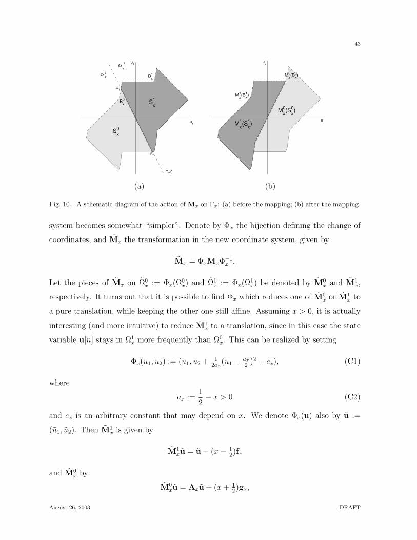
43

u1

u2

T=0

Sx0

Ω 0

x

Ω 1

x

Sx1 B

x0

Bx1

QT

PT

(a)

Mx0(S

x0)

Mx1(S

x1)

Mx0(B

x0)

Mx1(B

x1)

u1

u2

(b)

Fig. 10. A schematic diagram of the action of Mx on Γx: (a) before the mapping; (b) after the mapping.

system becomes somewhat “simpler”. Denote by Φx the bijection defining the change of

coordinates, and Mx the transformation in the new coordinate system, given by

Mx = ΦxMxΦ−1x .

Let the pieces of Mx on Ω0x := Φx(Ω

0x) and Ω1

x := Φx(Ω1x) be denoted by M0

x and M1x,

respectively. It turns out that it is possible to find Φx which reduces one of M0x or M1

x to

a pure translation, while keeping the other one still affine. Assuming x > 0, it is actually

interesting (and more intuitive) to reduce M1x to a translation, since in this case the state

variable u[n] stays in Ω1x more frequently than Ω0

x. This can be realized by setting

Φx(u1, u2) := (u1, u2 + 12ax

(u1 − ax

2)2 − cx), (C1)

where

ax :=1

2− x > 0 (C2)

and cx is an arbitrary constant that may depend on x. We denote Φx(u) also by u :=

(u1, u2). Then M1x is given by

M1xu = u + (x− 1

2)f ,

and M0x by

M0xu = Axu + (x + 1

2)gx,


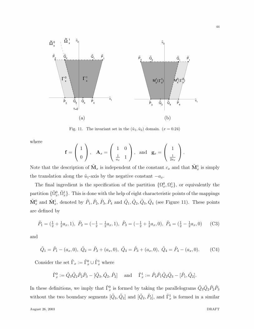
44

u1

u2

T=0

x0

Ω Ω

x1

Q2

Γ Γ

x0 x

1

Q1

Q4

Q3P

3

P1

P2

P4

~ ~ ~ ~

~ ~ ~ ~

~ ~ ~

~

(a)

u1

u2

Mx0(

x0)

Q2

Γ

Q1

Q4

Q3P

3

P1

P2

P4

~ ~ ~ ~

~ ~ ~ ~

Mx1(

x1)Γ

~

~

(b)

Fig. 11. The invariant set in the (u1, u2) domain. (x = 0.24)

where

f =

1

0

, Ax =

1 0

1ax

1

, and gx =

1

12ax

.

Note that the description of Mx is independent of the constant cx and that M1x is simply

the translation along the u1-axis by the negative constant −ax.

The final ingredient is the specification of the partition Ω0x, Ω

1x, or equivalently the

partition Ω0x, Ω

1x. This is done with the help of eight characteristic points of the mappings

M0x and M1

x, denoted by P1, P2, P3, P4 and Q1, Q2, Q3, Q4 (see Figure 11). These points

are defined by

P1 = (12

+ 12ax, 1), P2 = (−1

2− 1

2ax, 1), P3 = (−1

2+ 1

2ax, 0), P4 = (1

2− 1

2ax, 0) (C3)

and

Q1 = P1 − (ax, 0), Q2 = P2 + (ax, 0), Q3 = P3 + (ax, 0), Q4 = P4 − (ax, 0). (C4)

Consider the set Γx := Γ0x ∪ Γ1

x where

Γ0x := Q3Q2P2P3 − [Q3, Q2, P2] and Γ1

x := P4P1Q2Q3 − [P1, Q2].

In these definitions, we imply that Γ0x is formed by taking the parallelograms Q3Q2P2P3

without the two boundary segments [Q3, Q2] and [Q2, P2], and Γ1x is formed in a similar


45

manner. These two sets are illustrated in Figure 11(a). Note from the figure that Γx is

then simply the trapezoid P4P1P2P3 from which the upper boundary segment [P1, P2] has

been removed. Now, one can easily check that

M0x(Γ

0x) = P1Q1Q4P4 − [P1, Q1, Q4] and M1

x(Γ1x) = Q4Q1P2P3 − [Q1P2].

These sets are illustrated in Figure 11(b). One can easily see that M0x(Γ

0x)∪M1

x(Γ1x) = Γx.

If we choose the straight line passing through Q2 and Q3 as the boundary between Ω0x and

Ω1x, i.e.,

Ω1x =

(u1, u2) : u1 + ax(u2 − 3

2) + 1

2≥ 0

,

then we ensure that Γ0x ⊂ Ω0

x and Γ1x ⊂ Ω1

x. In this situation, we have Mx(Γx) = M0x(Γ

0x)∪

M1x(Γ

1x) = Γx. Back to the original space, the set Γx := Φ−1(Γx) then satisfies Mx(Γx) =

Γx. Because of the quadratic nature of Φx, it is clear that Γx has a boundary composed

of four parabolic pieces. This is illustrated in Figure 9. Because the boundary segment

[P1, P2] is excluded from Γx, the boundary parabola passing through P1 and P2 is excluded

from Γx.

To find the expression for T back in the original system of coordinates, we substitute

the expressions for u1, u2 and ax from (C1) and (C2). Then the resulting function T , up

to a scaling factor, is given by the expression (57) with

C(x) = 8(x− 12)cx − 3x2 + 11x− 7

4. (C5)

In this paper, the choice of C(x) does not matter. However, when dealing with time-

varying inputs, it is shown in [23] that it is interesting to choose C(x) so that the centroid of

Γx is located at (0, 0) regardless of x. In this situation, it is indeed numerically shown that

the resulting modulator becomes superior in performance to the one-bit linear-T second

order modulators. Since Γx is here entirely known analytically, such a value of C(x) is

easy to derive. We show in Appendix-E that this is achieved when C(x) = (7− 3x)x− 112

for x ∈ [0, 12).

D. Proof of Proposition IV.1

Proof: Property 1 can be checked in a straightforward manner using the explicit

parametric descriptions of the invariant sets given in the respective sections and in the



46

Appendix. Property 2 is a consequence of the fact that each of the invariant sets possesses a

boundary that is composed of a finite number of smooth curves, totaling a finite perimeter.

Hence the ε-neighborhood of each ∂Γx cover an area that decreases as O(ε) as ε → 0. The

uniformity of the constants M0 and C0 are guaranteed by the choice of the intervals I(D).

In particular, these intervals can be chosen to be [−12, 1

2], [−1

6, 1

6] and an arbitrary closed

subinterval of (−12, 1

2), respectively. Let us prove Property 3.

The L2 system: This was shown in Section IV-A.

The Q1 system: The invariant set is Γx = Φ−1x (P1P2P3P4) where the points Pi are given

in (C3) and Φx is given in (C1). From (C3), we derive the equations of the four linear

boundaries of the parallelograms P1P2P3P4 and obtain

(P1P2) : u2 = 1 , (P2P3) : u2 = − 12ax

u1 − 12ax

+ 12,

(P3P4) : u2 = 0 , (P1P4) : u2 = + 12ax

u1 − 12ax

+ 12.

By writing (u1, u2) = Φx(u1, u2) and applying (C1), we derive the equations of the four

parabolic boundaries of Φ−1x (P1P2P3P4) and obtain

(P1P2) : u2 = − 12ax

(u1 − ax

2 )2 + cx + 1 , (P2P3) : u2 = − 12ax

(u1 − ax

2 )2 + cx − 12ax

u1 − 12ax

+ 12 ,

(P3P4) : u2 = − 12ax

(u1 − ax

2 )2 + cx , (P1P4) : u2 = − 12ax

(u1 − ax

2 )2 + cx + 12ax

u1 − 12ax

+ 12 .

One can then easily check that the four above parabolas satisfy the following relations:

(P1P4) = (P1P2) + (1, 0),

(P3P4) = (P1P2)− (0, 1),

(P2P3) = (P1P2)− (1, 1).

(D1)

This can be also graphically seen in Figure 9. This is sufficient to prove Property 3 for the

Q1 system. A graphical representation of the tiling property is shown in the same figure.

The L1 system: Proving the tiling property of the invariant set Γx described in Section

IV-B is a tedious process. Here, we will only point out boundary relations similar to (D1).

Given n vertices R1, R2, · · · , Rn, let us use the notation [R1, R2, · · · , Rn] to designate the

union of the segments [Ri−1, Ri] for i = 2, · · · , n. By using Table II, one can see that

[P2k−1, Q2] = [P ′2k−1, Q

′2] + (1, 0),

[P2, P4, · · · , P2k−2, Q1, P1, P3, · · · , P2k−3] = [P ′2, P

′4, · · · , P ′

2k−2, Q′1, P

′1, P

′3, · · · , P ′

2k−3]− (0, 1),

[Q0, P0] = [Q′0, P

′0]− (1, 1).

We illustrate these three relations by the three arrows in Figure 8(b).


47

E. On the analysis of the quadratic scheme: zero-centroid setting of C(x)

Let us call Gx = (u1,x, u2,x) the centroid point of Γx and write u = (u1, u2) in general.

We have

Gx =

∫u∈Γx

u du =

∫u∈Φ(Γx)

Φ−1(u) du.

In the last equality, we have used the fact that du = du since the transformation Φ

from (C1) conserves measure. We know from Section IV-C that Φ(Γx) is the trapezoid

P1P2P3P4. From (C2) and the explicit coordinates of its vertices given in (C3) and (C4),

we have

Φ(Γx) =(u1, u2) : 0 ≤ u2 ≤ 1 and |u1| ≤ 1

2+ ax(u2 − 1

2)

.

From (C1), one easily derives that

Φ−1(u) = (u1, u2 − 12ax

(u1 − ax

2)2 + cx

).

Consequently, the first component of Gx is u1,x =∫u∈Φ(Γx)

u1 du. Since Φ(Γx) is clearly

symmetrical with respect to the u2-axis, we already have u1,x = 0. The second component

of Gx is equal to

u2,x =

∫ 1

u2=0

∫ 12+ax(u− 1

2)

u1=− 12−ax(u− 1

2)

(u2 − 1

2ax(u1 − ax

2)2 + cx

)du1du2 = 1

2− 1

24ax+ cx.

The component ux will then be systematically equal to 0 by choosing cx = 124ax

− 12. Using

(C2) and (C5), this implies that C(x) = (7− 3x)x− 112

.

acknowledgments

The authors would like to thank Ingrid Daubechies, Ron DeVore, Ozgur Yılmaz and

Jade Vinson for interesting discussions on the topic of this paper, and the anonymous

referees for their helpful comments and suggestions on the presentation. S.G. would like

to thank Institute for Advanced Study and Courant Institute for their hospitality during

the writing stage of this work.

References

[1] J. C. Candy and G. C. Temes, Eds., Oversampling Delta-Sigma Data Converters: Theory, Design and

Simulation, IEEE Press, 1992.


48

[2] W. Chou, T. H. Meng, and R. M. Gray, “Time Domain Analysis of Sigma Delta Modulation,” Proceedings

ICASSP-90, Int. Conf. on Acoustics, Speech and Signal Processing, vol. 3, pp. 1751–1754, Albuquerque, NM,

April 1990.

[3] W. Chou, P. W. Wong, and R. M. Gray, “Multistage sigma-delta modulation,” IEEE Trans. Inform. Theory,

vol. 35, pp. 784–796, July 1989.

[4] I. Daubechies and R. A. DeVore, “Reconstructing a bandlimited function from very coarsely quantized data:

A family of stable sigma-delta modulators of arbitrary order,” Ann. of Math., vol. 158, no. 2, pp. 643–674,

Sept. 2003.

[5] M. Drmota and R. F. Tichy, Sequences, Discrepancies and Applications, Springer, 1997.

[6] R. M. Gray, “Spectral analysis of quantization noise in a single-loop sigma-delta modulator with dc input,”

IEEE Transactions on Communications, vol. 37, pp. 588–599, June 1989.

[7] R. M. Gray, W. Chou, and P.-W. Wong, “Quantization noise in single-loop sigma-delta modulation with

sinusoidal input,” IEEE Transactions on Communications, vol. COM-37, pp. 956–968, Sept. 1989.

[8] C. S. Gunturk, “Improved error estimates for first order sigma-delta modulation,” in Proceedings of the

International Workshop on Sampling Theory and Applications, SampTA’99, August 1999, pp. 171–176, Loen,

Norway.

[9] C. S. Gunturk, Harmonic Analysis of Two Problems in Signal Quantization and Compression, Ph.D. thesis,

Princeton University, 2000.

[10] C. S. Gunturk, “Approximating a Bandlimited Function Using Very Coarsely Quantized Data: Improved

Error Estimates in Sigma-Delta Modulation”, J. Amer. Math. Soc., posted on August 1, 2003, PII S 0894-

0347(03)00436-3 (to appear in print).

[11] C. S. Gunturk, J. Lagarias, and V. Vaishampayan, “On the robustness of single loop sigma-delta modulation,”

IEEE Transactions on Information Theory., July 2001.

[12] N. He, F. Kuhlmann, and A. Buzo, “Double-loop sigma-delta modulation with dc input,” IEEE Trans.

Commun, vol. 38, pp. 487–495, April 1990.

[13] N. He, F. Kuhlmann, and A. Buzo, “Multi-loop sigma-delta quantization,” IEEE Trans. Inform. Theory,

vol. 38, pp. 1015–1028, May 1992.

[14] D. F. Hoschele, Jr., Analog-to-Digital and Digital-to-Analog Conversion Techniques, John Wiley & Sons,

1994.

[15] H. Inose and Y. Yasuda, “A unity bit coding method by negative feedback,” Proceedings of the IEEE, vol.

51, pp. 1524–1535, Nov 1963.

[16] L. Kuipers and H. Niederreiter, Uniform Distribution of Sequences, Wiley, 1974.

[17] M. Laczkovich, “Discrepancy estimates for sets with small boundary,” Stud. Sci. Math. Hung., vol. 30, pp.

105–109, 1995.

[18] H. Niederreiter, “Application of diophantine approximations to numerical integration,” in Diophantine

Approximation and its Applications, C. F. Osgood, Ed., pp. 129–199. Academic Press, 1973.

[19] S. R. Norsworthy, R. Schreier, and G. C. Temes, Eds., Delta-Sigma Data Converters: Theory, Design and

Simulation, IEEE Press, 1996.

[20] W. Parry, Topics in Ergodic Theory, Cambridge University Press, 1981.

[21] R. Schreier, M. V. Goodson, and B. Zhang, “An algorithm for computing convex positively invariant sets for

delta-sigma modulators,” IEEE Trans. on Circuits and Systems, I, vol. 44, pp. 38–44, January 1997.























https://www.researchgate.net/publication/268497495_Application_of_diophantine_approximations_to_numerical_integration?el=1_x_8&enrichId=rgreq-4276f12f34a15f58a8032eece18022b7-XXX&enrichSource=Y292ZXJQYWdlOzMwODUwMjU7QVM6MTIyMTg5NjkzMDY3MjY2QDE0MDYxNDM3MDE5NzM=

https://www.researchgate.net/publication/268497495_Application_of_diophantine_approximations_to_numerical_integration?el=1_x_8&enrichId=rgreq-4276f12f34a15f58a8032eece18022b7-XXX&enrichSource=Y292ZXJQYWdlOzMwODUwMjU7QVM6MTIyMTg5NjkzMDY3MjY2QDE0MDYxNDM3MDE5NzM=



https://www.researchgate.net/publication/3080435_On_the_robustness_of_single-loop_sigma-delta_modulation?el=1_x_8&enrichId=rgreq-4276f12f34a15f58a8032eece18022b7-XXX&enrichSource=Y292ZXJQYWdlOzMwODUwMjU7QVM6MTIyMTg5NjkzMDY3MjY2QDE0MDYxNDM3MDE5NzM=

https://www.researchgate.net/publication/3080435_On_the_robustness_of_single-loop_sigma-delta_modulation?el=1_x_8&enrichId=rgreq-4276f12f34a15f58a8032eece18022b7-XXX&enrichSource=Y292ZXJQYWdlOzMwODUwMjU7QVM6MTIyMTg5NjkzMDY3MjY2QDE0MDYxNDM3MDE5NzM=

https://www.researchgate.net/publication/266013032_Topics_in_Ergodic_Theory?el=1_x_8&enrichId=rgreq-4276f12f34a15f58a8032eece18022b7-XXX&enrichSource=Y292ZXJQYWdlOzMwODUwMjU7QVM6MTIyMTg5NjkzMDY3MjY2QDE0MDYxNDM3MDE5NzM=






https://www.researchgate.net/publication/3077410_Multistage_Sigma-Delta_Modulation?el=1_x_8&enrichId=rgreq-4276f12f34a15f58a8032eece18022b7-XXX&enrichSource=Y292ZXJQYWdlOzMwODUwMjU7QVM6MTIyMTg5NjkzMDY3MjY2QDE0MDYxNDM3MDE5NzM=

https://www.researchgate.net/publication/3077410_Multistage_Sigma-Delta_Modulation?el=1_x_8&enrichId=rgreq-4276f12f34a15f58a8032eece18022b7-XXX&enrichSource=Y292ZXJQYWdlOzMwODUwMjU7QVM6MTIyMTg5NjkzMDY3MjY2QDE0MDYxNDM3MDE5NzM=

49

[22] N. T. Thao, “Vector Quantization Analysis of Σ∆ Modulation,” IEEE Transactions on Signal Processing,

vol.44, pp.808-817, Apr. 1996.

[23] N. T. Thao, “MSE behavior and centroid function of mth order asymptotic Σ∆ modulators,” IEEE Trans.

Circuits and Systems II, 2001, submitted.

[24] N. T. Thao and C. S. Gunturk, “Ergodic Dynamics in Σ∆ Quantization: Tiling Invariant Sets and Spectral

Analysis of Error,” arXiv:math.DS/0308223, http://arXiv.org/abs/math.DS/0308223.

[25] N. T. Thao and M. Vetterli, “Deterministic Analysis of Oversampled A/D Conversion and Decoding Im-

provement Based on Consistent Estimates,” IEEE Transactions on Signal Processing, vol.42, pp.519-531,

Mar. 1994.

[26] O. Yılmaz, “Stability analysis for several sigma-delta methods of coarse quantization of bandlimited func-

tions,” Constructive Approximation, 18 (2002), no. 4, 599–623.











Refined error analysis in second-order Sigma-Delta modulation with constant inputs

Documents