SENTINEL‐3 OPTICAL PRODUCTS AND ALGORITHM DEFINITION OLCI Level 2 Algorithm Theoretical Basis Document Transparency products Ref: S3‐L2‐SD‐03‐ C16‐ACR‐ATBD Issue: 1.0 Date: 03/05/10 OLCI Level 2 Algorithm Theoretical Basis Document Transparency products Kd(490) Secchi disk depth Heated layer depth DOCUMENT REF: S3‐L2‐SD‐03‐C16‐ACR‐ATBD DELIVERABLE REF: SD‐03‐C16 VERSION: 1.0

Welcome message from author
This document is posted to help you gain knowledge. Please leave a comment to let me know what you think about it! Share it to your friends and learn new things together.
Transcript

SENTINEL‐3 OPTICAL PRODUCTS AND ALGORITHM
DEFINITION
OLCI Level 2 Algorithm Theoretical Basis Document Transparency products
Ref: S3‐L2‐SD‐03‐ C16‐ACR‐ATBD Issue: 1.0 Date: 03/05/10
OLCI Level 2
Algorithm Theoretical Basis Document
Transparency products
Kd(490) Secchi disk depth Heated layer depth
DOCUMENT REF: S3‐L2‐SD‐03‐C16‐ACR‐ATBD DELIVERABLE REF: SD‐03‐C16 VERSION: 1.0

SENTINEL‐3 OPTICAL PRODUCTS AND ALGORITHM
DEFINITION
OLCI Level 2 Algorithm Theoretical Basis Document Transparency products
Ref: S3‐L2‐SD‐03‐ C16‐ACR‐ATBD Issue: 1.0 Date: 03/05/10 Page :
All rights reserved ACRI-ST 2010 CONFIDENTIAL
i
Document Signature Table
Name Function Company Signature Date
Prepared A. Mangin Research Engineer
ACRI‐ST
Approved L. Bourg OLCI expert ACRI‐ST
Released O. Fanton d’Andon
OLCI coordinator ACRI‐ST
Change record
Issue Date Description Change pages
1.0 03/05/2010 Version 1 to close CDR RIDs N° 193, 114 Initial version
Distribution List
Organisation To Nb. of copies
ESA Philippe Goryl, Alessandra Buongiorno and Carla
Santella 1
EUMETSAT Vincent Fournier‐Sicre, Vincenzo Santacesaria 1
S3 Optical OLCI team ARGANS, ACRI‐ST 1
SENTINEL‐3 OPTICAL PRODUCTS AND ALGORITHM
DEFINITION
OLCI Level 2 Algorithm Theoretical Basis Document Transparency products
Ref: S3‐L2‐SD‐03‐ C16‐ACR‐ATBD Issue: 1.0 Date: 03/05/10 Page :
All rights reserved ACRI-ST 2010 CONFIDENTIAL
ii
TABLE OF CONTENTS
1. INTRODUCTION .....................................................................................................................1
1.1 PURPOSE AND SCOPE..............................................................................................................1 1.2 ALGORITHM IDENTIFICATION....................................................................................................1 1.3 ACRONYMS ..........................................................................................................................1 1.4 SYMBOLS .............................................................................................................................2
2. ALGORITHM OVERVIEW........................................................................................................3
2.1 OBJECTIVES ..........................................................................................................................3
3. THE DIFFUSE ATTENUATION COEFFICIENT AT 490 NM (KD(490))..................4
3.1 KD(490) ALGORITHM.........................................................................................................4 3.2 KD(490) VALIDATION ........................................................................................................5
4. SECCHI DISK DEPTH.......................................................................................................6
4.1 SECCHI DISK DEPTH ALGORITHM .......................................................................................6 4.1.1 Background...............................................................................................................6 4.1.2 Computation of (c+Kd).............................................................................................6 Computation of .......................................................................................................7
4.2 SECCHI DISK DEPTH VALIDATION ......................................................................................8 4.3 SECCHI DISK DEPTH ERROR BARS ....................................................................................10
5. HEATED LAYER DEPTH...............................................................................................11
5.1 HEATED LAYER DEPTH ALGORITHM ................................................................................11 5.2 HEATED LAYER DEPTH VALIDATION................................................................................12
6. ASSUMPTIONS AND LIMITATIONS ..........................................................................14
7. REFERENCES...................................................................................................................15

SENTINEL‐3 OPTICAL PRODUCTS AND ALGORITHM
DEFINITION
OLCI Level 2 Algorithm Theoretical Basis Document Transparency products
Ref: S3‐L2‐SD‐03‐ C16‐ACR‐ATBD Issue: 1.0 Date: 03/05/10 Page:iii
All rights reserved ACRI-ST 2010 CONFIDENTIAL
LIST OF FIGURES
Figure 1‐ Validation of the OK2‐555 algorithm against the NOMAD in situ data set (Werdell and
Bailey, 2005) ............................................................................................................................................ 5
Figure 2‐ Validation of the ZSD for various match‐ups and for (up) MERIS and (down) MODIS .............. 9
Figure 3‐ Error bar estimates from validation of ZSD formulation vs in situ truth ................................. 10
Figure 4‐ ZHL monthly product – December 2003 ................................................................................. 12
Figure 5‐ Proposed Algorithm for Kd(PAR) as a function of Kd(490) vs experimental observations..... 13
LIST OF TABLES
Table 1– Available data set for evaluation and validation of Secchi disk depth ..................................... 8
Table 2– Results of matchup with MERIS and MODIS for validation of Secchi disk depth...................... 8

SENTINEL‐3 OPTICAL PRODUCTS AND ALGORITHM
DEFINITION
OLCI Level 2 Algorithm Theoretical Basis Document Transparency products
Ref: S3‐L2‐SD‐03‐ C16‐ACR‐ATBD Issue: 1.0 Date: 03/05/10 Page:1
All rights reserved ACRI-ST 2010 CONFIDENTIAL
1. INTRODUCTION
1.1 Purpose and scope
This Algorithm Theoretical Basis document (ATBD) is written for the Ocean and Land Colour Imager (OLCI) of the Earth Observation Mission SENTINEL 3 of the European Space Agency (ESA). The purpose of this document is to lay out algorithms for the sea water transparency products. As much as possible, basic principles of the algorithm and the description of their various segments will refer to publications in the peer‐reviewed scientific literature. When such literature exists, minimum information will be provided here for the sake of clarity, and the reader will be referred to the relevant literature for further information.
1.2 Algorithm identification
This algorithm is identified under reference “SD‐03‐C16” in the sentinel‐3 OLCI documentation.
1.3 Acronyms
ATBD Algorithm Theoretical Basis Document
CWOC Clear Water Ocean Colour
ESA European Space Agency
MERIS Medium Resolution Imaging Spectrometer
OLCI Ocean and Land Color Imager
PAR Photosynthetic Available Radiation
SENTINEL 3 Third series of “sentinel” (ESA satellites)

SENTINEL‐3 OPTICAL PRODUCTS AND ALGORITHM
DEFINITION
OLCI Level 2 Algorithm Theoretical Basis Document Transparency products
Ref: S3‐L2‐SD‐03‐ C16‐ACR‐ATBD Issue: 1.0 Date: 03/05/10 Page:2
All rights reserved ACRI-ST 2010 CONFIDENTIAL
1.4 Symbols
Symbol definition Dimension / units
Geometry, wavelengths
Wavelength nm
s Sun zenith angle (s = cos(s)) degrees v Satellite viewing angle (v = cos(v)) degrees Azimuth difference between the sun‐pixel and pixel‐sensor degrees half vertical planes Water properties
Chl Chlorophyll concentration mg m‐3
a() Total absorption coefficient m‐1
b() Total scattering coefficient m‐1
bb() Total backscattering coefficient m‐1
bbp() Total backscattering coefficient due to particles m‐1
bw() Total water scattering coefficient m‐1
bbw() Total backscattering coefficient due to pure water m‐1
R(, 0-) Diffuse reflectance at null depth, or irradiance ratio (Eu / Ed) dimensionless (upward and downward irradiances, respectively)
Kd() Diffuse attenuation coefficient for the downward plane m‐1
irradiance
Kd(PAR) Diffuse attenuation coefficient for the downward plane m‐1
Irradiance for the whole visible spectrum
Kw() Diffuse attenuation coefficient for the downward plane m‐1
irradiance, for seawater only
Q(,s,v,) Factor describing the bidirectional character of R(, 0-) sr subscript 0 when s = v = 0 w() Normalised water‐leaving reflectance (i.e., the reflectance if
there were no atmosphere, and for s = v = 0) dimensionless Air‐water interface
)( Geometrical factor, accounting for all refraction and reflection dimensionless
effects at the air‐sea interface (Morel and Gentili, 1996) Transparency products CSD Contrast between the Secchi disk and the surrounding water compared to the
surrounding water r albedo of the Secchi disk
Cobs Detection threshold as can be detected by a human eye ZSD Secchi Disk Depth m (ZSD) Standard deviation of the Secchi Disk Depth m

SENTINEL‐3 OPTICAL PRODUCTS AND ALGORITHM
DEFINITION
OLCI Level 2 Algorithm Theoretical Basis Document Transparency products
Ref: S3‐L2‐SD‐03‐ C16‐ACR‐ATBD Issue: 1.0 Date: 03/05/10 Page:3
All rights reserved ACRI-ST 2010 CONFIDENTIAL
2. ALGORITHM OVERVIEW
2.1 Objectives
The objective is to derive several ocean colour products characterising the transparency from the spectrum of the normalised water‐leaving reflectances. The following products are derived here:
The diffuse attenuation coefficient at 490 nm, expressed in units of m‐1.
The water transparency expressed under the form of a Secchi depth in units of m.
The depth of light penetration into the sea water expressed as a heated layer depth in units
of m.
Notes:
The diffuse attenuation coefficient and the Secchi disk depth are derived from various combinations of the fully normalized water‐leaving reflectances.

SENTINEL‐3 OPTICAL PRODUCTS AND ALGORITHM
DEFINITION
OLCI Level 2 Algorithm Theoretical Basis Document Transparency products
Ref: S3‐L2‐SD‐03‐ C16‐ACR‐ATBD Issue: 1.0 Date: 03/05/10 Page:4
All rights reserved ACRI-ST 2010 CONFIDENTIAL
3. The diffuse attenuation coefficient at 490 nm (Kd(490))
3.1 Kd(490) algorithm The diffuse attenuation coefficient for the downward plane irradiance at wavelength and at a given depth z is defined as:
( ) 1/ ( , ) ( , ) /d d dK E z dE z dz or ( ) ( , ) /d dK d lnE z dz (1)
Many realisations of this coefficient are possible, as a function of the depth range over which it is computed. It can be a local coefficient around a given small depth interval between any depths z1 and z2 :
12
21 ),(/),(log)(
zz
zEzEK dd
d
(2)
It can be computed for the upper layer defined from below the surface (0‐) to a given depth z:
z
)0(E/)z(ElogK dd
d
(3)
It can also be an Ed‐weighted average value computed over a certain depth z, e.g., the 1% light level
(Kirk, 2003)
dzzE
dzzEzK
K z
d
z
dd
avd
0
0,
),(
),(),(
)(
(4)
Practically speaking, the Kd's found in in situ data bases are essentially of the second category. The reason is simply that measuring properly Ed(Z) at sea requires that the irradiance sensor is placed at
a depth where the irradiance fluctuations due to surface waves are small enough (or even absent). This depth can be as large as ~30 meters in clear waters. Then this Ed(z) measurement is combined
with the downward irradiance measured above the surface after it is multiplied by the transmission
across the air‐sea interface, which provides Ed(0‐), in order to get the Kd as per Eq (5) above.
We propose here to use the “OK2‐560” algorithm proposed by Morel et al. (2007). It is based on the 490‐560 reflectance ratio, and has the form:
n
x
xxA
0560,49010 )(log
wd 10)490(K=)490(K
(5)
Where Kw(490) is 0.0166 m‐1, 490,560 is the ratio of the normalized water‐leaving reflectance at
490 and 560 nm, and the n+1=5 coefficients Ax have the values : A0: ‐0,82789 A1: ‐1,64219 A2: 0,90261 A3:‐1,62685 A4: 0,088504

SENTINEL‐3 OPTICAL PRODUCTS AND ALGORITHM
DEFINITION
OLCI Level 2 Algorithm Theoretical Basis Document Transparency products
Ref: S3‐L2‐SD‐03‐ C16‐ACR‐ATBD Issue: 1.0 Date: 03/05/10 Page:5
All rights reserved ACRI-ST 2010 CONFIDENTIAL
3.2 Kd(490) validation The expression of Kd(490) has been validated (Morel et al. 2007) against independent in situ measurements (the NOMAD database – Werdell and Bailey 2005) and indicates very good agreement (see figure below) with a determination coefficient of 0,921 and no bias.
Figure 1‐ Validation of the OK2‐555 algorithm against the NOMAD in situ data set (Werdell and Bailey, 2005)

SENTINEL‐3 OPTICAL PRODUCTS AND ALGORITHM
DEFINITION
OLCI Level 2 Algorithm Theoretical Basis Document Transparency products
Ref: S3‐L2‐SD‐03‐ C16‐ACR‐ATBD Issue: 1.0 Date: 03/05/10 Page:6
All rights reserved ACRI-ST 2010 CONFIDENTIAL
4. Secchi disk depth
4.1 Secchi disk depth algorithm 4.1.1 Background The Secchi disk depth ZSD is, by nature, a good characterisation of the vertical visibility underwater. It is linked to two optical parameters; the vertical diffuse attenuation coefficient Kd (m
‐1) which gives the quantity of light available in the water column and the attenuation coefficient c (m‐1) that determines the propagation of light through the water mass.
Tyler (1968) has given a simplified expression of the Secchi disk depth :
SDd ZKcSDObs eCC )( (1)
In which SDC is the contrast between the Secchi disk and the surrounding water compared to the
surrounding water and CObs is the detection threshold as can be detected by a human eye. ZSD is the maximum depth to which Secchi disk can be observed.
The above expression is equivalent to:
)()(
log
dd
SD
Obs
SD KcKc
C
C
Z
(2)
The development that was done and published in (Doron et al. 2007) and which is the baseline for this ATBD is based on the determination of both part of this last equation (the numerator which is purely due to observation condition and the denominator which is linked to water optical properties) to estimate the Secchi disk depth.
4.1.2 Computation of (c+Kd) The computation of the attenuation part of expression (2) is summarised here below.
(i) The reflectances used in the following are first expressed underwater starting from the fully normalised water leaving reflectances as follows:
rQ
R
w
w
)0( (3)
in which, =0,529 , Q=4 and r =0,48
(ii) The particle backscattering coefficient bbp (m‐1) is computed by using sub‐surface reflectances
at 560 nm and the ratio of reflectances at 490 nm and 560 nm.
)560(,
)490(
)560()490( R
R
Rfunctionbbp (3’)
SENTINEL‐3 OPTICAL PRODUCTS AND ALGORITHM
DEFINITION
OLCI Level 2 Algorithm Theoretical Basis Document Transparency products
Ref: S3‐L2‐SD‐03‐ C16‐ACR‐ATBD Issue: 1.0 Date: 03/05/10 Page:7
All rights reserved ACRI-ST 2010 CONFIDENTIAL
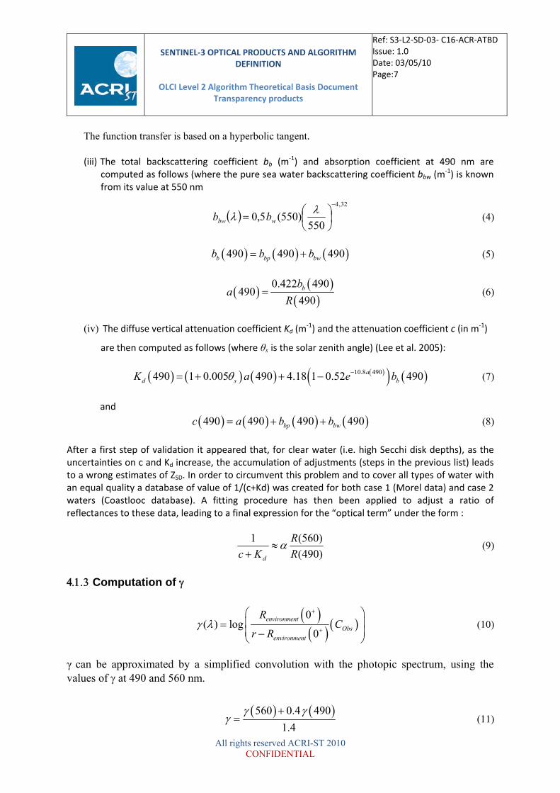
The function transfer is based on a hyperbolic tangent. (iii) The total backscattering coefficient bb (m
‐1) and absorption coefficient at 490 nm are computed as follows (where the pure sea water backscattering coefficient bbw (m
‐1) is known from its value at 550 nm
32,4
550)550(5,0
wbw bb (4)
490 490 490b bp bwb b b (5)
0.422 490490
490bb
aR
(6)
(iv) The diffuse vertical attenuation coefficient Kd (m‐1) and the attenuation coefficient c (in m‐1)
are then computed as follows (where θs is the solar zenith angle) (Lee et al. 2005):
10.8 490490 1 0.005 490 4.18 1 0.52 490ad s bK a e b (7)
and
490 490 490 490bp bwc a b b (8)
After a first step of validation it appeared that, for clear water (i.e. high Secchi disk depths), as the uncertainties on c and Kd increase, the accumulation of adjustments (steps in the previous list) leads to a wrong estimates of ZSD. In order to circumvent this problem and to cover all types of water with an equal quality a database of value of 1/(c+Kd) was created for both case 1 (Morel data) and case 2 waters (Coastlooc database). A fitting procedure has then been applied to adjust a ratio of reflectances to these data, leading to a final expression for the “optical term” under the form :
)490(
)560(1
R
R
Kc d
(9)
Computation of
0( ) log
0
environment
Obs
environment
RC
r R
(10)
γ can be approximated by a simplified convolution with the photopic spectrum, using the values of at 490 and 560 nm.
560 0.4 490
1.4
(11)
SENTINEL‐3 OPTICAL PRODUCTS AND ALGORITHM
DEFINITION
OLCI Level 2 Algorithm Theoretical Basis Document Transparency products
Ref: S3‐L2‐SD‐03‐ C16‐ACR‐ATBD Issue: 1.0 Date: 03/05/10 Page:8
All rights reserved ACRI-ST 2010 CONFIDENTIAL
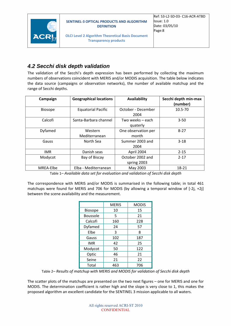
4.2 Secchi disk depth validation The validation of the Secchi’s depth expression has been performed by collecting the maximum numbers of observations coincident with MERIS and/or MODIS acquisition. The table below indicates the data source (campaigns or observation networks), the number of available matchup and the range of Secchi depths.
Campaign Geographical locations Availability Secchi depth min‐max (number)
Biosope Equatorial Pacific October ‐ December 2004
10.5‐70
Calcofi Santa‐Barbara channel Two weeks – each quaterly
3‐50
Dyfamed Western Mediterranean
One observation per month
8‐27
Gauss North Sea Summer 2003 and 2004
3‐18
IMR Danish seas April 2004 2‐15
Modycot Bay of Biscay October 2002 and spring 2003
2‐17
MREA‐Elbe Elba ‐ Mediterranean May 2003 18‐21
Table 1– Available data set for evaluation and validation of Secchi disk depth The correspondence with MERIS and/or MODIS is summarised in the following table; in total 461 matchups were found for MERIS and 706 for MODIS (by allowing a temporal window of [‐2j, +2j] between the scene availability and the measurement.
MERIS MODIS
Biosope 10 15
Boussole 5 21
Calcofi 160 228
Dyfamed 24 57
Elbe 3 8
Gauss 102 187
IMR 42 25
Modycot 50 122
Optic 46 21
Seine 21 22
Total 463 706
Table 2– Results of matchup with MERIS and MODIS for validation of Secchi disk depth The scatter plots of the matchups are presented on the two next figures – one for MERIS and one for MODIS. The determination coefficient is rather high and the slope is very close to 1, this makes the proposed algorithm an excellent candidate for the SENTINEL 3 mission applicable to all waters.

SENTINEL‐3 OPTICAL PRODUCTS AND ALGORITHM
DEFINITION
OLCI Level 2 Algorithm Theoretical Basis Document Transparency products
Ref: S3‐L2‐SD‐03‐ C16‐ACR‐ATBD Issue: 1.0 Date: 03/05/10 Page:9
All rights reserved ACRI-ST 2010 CONFIDENTIAL
Validation - Secchi depth (MERIS)MERIS 463 points (R2=0.76; slope 1.03)
0
5
10
15
20
25
30
35
40
45
50
0 5 10 15 20 25 30 35 40 45 50
Secchi depth In situ (m)
Sec
chi
dep
th (
fro
m M
ER
IS)
(m)
Validation - Secchi depth MODIS MODIS 706 points (R2=0.72)
0
5
10
15
20
25
30
35
40
45
50
0 5 10 15 20 25 30 35 40 45 50
Secchi depth In situ (m)
Sec
chi
dep
th (
fro
m M
OD
IS)
(m)
Figure 2‐ Validation of the ZSD for various match‐ups and for (up) MERIS and (down) MODIS

SENTINEL‐3 OPTICAL PRODUCTS AND ALGORITHM
DEFINITION
OLCI Level 2 Algorithm Theoretical Basis Document Transparency products
Ref: S3‐L2‐SD‐03‐ C16‐ACR‐ATBD Issue: 1.0 Date: 03/05/10 Page:10
All rights reserved ACRI-ST 2010 CONFIDENTIAL
4.3 Secchi disk depth error bars
The quality of the Secchi disk depth has been derived from the validation dataset, described in the previous section. The analysis has been performed for several classes of depth (by layer of 5 meters) in order to derive the level of accuracy that could be applied to SENTINEL 3 outputs. Since no real bias is observed, an analytical expression for the uncertainties (one sigma) is proposed as follows.
524,0)log(686,1)( SDSD ZZ (12)
y = 1.6854Ln(x) + 0.5244R2 = 0.8641
0
1
2
3
4
5
6
7
0 5 10 15 20 25 30
Profondeur de Secchi (m)
Eca
rt t
ype
Sta
nda
rd d
evi
atio
n
Secchi depth (m)
y = 1.6854Ln(x) + 0.5244R2 = 0.8641
0
1
2
3
4
5
6
7
0 5 10 15 20 25 30
Profondeur de Secchi (m)
Eca
rt t
ype
Sta
nda
rd d
evi
atio
n
Secchi depth (m)
Figure 3‐ Error bar estimates from validation of ZSD formulation vs in situ truth

SENTINEL‐3 OPTICAL PRODUCTS AND ALGORITHM
DEFINITION
OLCI Level 2 Algorithm Theoretical Basis Document Transparency products
Ref: S3‐L2‐SD‐03‐ C16‐ACR‐ATBD Issue: 1.0 Date: 03/05/10 Page:11
All rights reserved ACRI-ST 2010 CONFIDENTIAL
5. Heated layer depth
5.1 Heated layer depth algorithm The heated layer depth is the sea surface layer that is impacted by the solar heat flux. It is a concept directly based on the light penetration for the whole solar spectrum and thus directly linked to the vertical attenuation of the light. It is proposed to be computed through the knowledge of the vertical diffuse attenuation coefficient Kd at 490 nm (Morel et al. 2007)
)()()()( ewd chlKK (13)
with: Kw(490) = 0.0166 m-1
490 = 0.08349 e(490) = 0.63303
From this knowledge, the heated layer depth (ZHL) is directly computed using the following equation.
PARKZ
dhl
2
(14)
with :
490
00121.0490874.00665.0
ddd K
KPARK (15)
This algorithm is implemented and is used operationally in GlobColour. Here below is an example of a global map of heated layer depth (monthly average).

SENTINEL‐3 OPTICAL PRODUCTS AND ALGORITHM
DEFINITION
OLCI Level 2 Algorithm Theoretical Basis Document Transparency products
Ref: S3‐L2‐SD‐03‐ C16‐ACR‐ATBD Issue: 1.0 Date: 03/05/10 Page:12
All rights reserved ACRI-ST 2010 CONFIDENTIAL
Figure 4‐ ZHL monthly product – December 2003
5.2 Heated layer depth validation By construction, the Zhl directly depends on the Kd(PAR) which is a measurable quantity. The validation of the former is thus based on the validity of the latter. Here below is a comparison (extracted from Morel et al. 2007) between the formulation (13) and an independent database; the SCAPA archive (Self‐Consistent AOP Profiles Archive;S.B. Hooker) This database was created from an extensive set of field campaigns throughout the world ocean (McClain et al., 2004), primarily (albeit not exclusively) in Case‐1 waters. The free‐fall multichannel sensor profilers (measuring upward radiance and irradiance, and downward irradiance) were operated according to strategies (Hooker & Maritorena, 2000) which are in strict adherence to the Ocean Optics Protocols (Mueller, 2003); this includes a rigorous quality control of the data (acquisition and processing), and a set of quality assurance procedures during the sensor calibration. The radiometric calibration facilities are traceable to the National Institute of Standards and Technology (Hooker et al., 2002). The figure below indicates a good agreement between the proposed algorithm and an independent dataset.

SENTINEL‐3 OPTICAL PRODUCTS AND ALGORITHM
DEFINITION
OLCI Level 2 Algorithm Theoretical Basis Document Transparency products
Ref: S3‐L2‐SD‐03‐ C16‐ACR‐ATBD Issue: 1.0 Date: 03/05/10 Page:13
All rights reserved ACRI-ST 2010 CONFIDENTIAL
Figure 5‐ Proposed Algorithm for Kd(PAR) as a function of Kd(490) vs experimental observations

SENTINEL‐3 OPTICAL PRODUCTS AND ALGORITHM
DEFINITION
OLCI Level 2 Algorithm Theoretical Basis Document Transparency products
Ref: S3‐L2‐SD‐03‐ C16‐ACR‐ATBD Issue: 1.0 Date: 03/05/10 Page:14
All rights reserved ACRI-ST 2010 CONFIDENTIAL
6. ASSUMPTIONS AND LIMITATIONS
The algorithm proposed for the Secchi depth is valid for all types of waters. The reader is referred more specifically to Doron et al. (2006) for a detailed discussion about the Secchi depth algorithm.
The -factor is impacted by the sea‐state, the sun irradiance and the cloud coverage. Some developments have been done with Hydrolight for the marine optical part. For effective sun irradiance over the scene, two models have been used, the first is RADTRAN (see Gregg and Carder, 1990). The second model computes the normalised distribution in all directions (Harrison and Coombes, 1988). The computations have been done for a range of wind speed values, solar zenith angles and cloud coverage. The impact would a few percent overestimate with increasing wind speed under clear sky conditions (which are the nominal conditions to apply the algorithm). The algorithms proposed for Kd and ZHL are valid above Case 1 waters, which means that they should be used with caution when applied over Case 2 waters. The same comment is valid for any other “non‐nominal” conditions of applications, including but not being limited to, coccolithophorid blooms, residual, non‐identified, sun glint, non‐corrected adjacency effects, cloud shadows and unfiltered thin clouds. For the Kd and ZHL algorithms, the reader is referred more specifically to Morel
et al. (2007) for a detailed discussion.

SENTINEL‐3 OPTICAL PRODUCTS AND ALGORITHM
DEFINITION
OLCI Level 2 Algorithm Theoretical Basis Document Transparency products
Ref: S3‐L2‐SD‐03‐ C16‐ACR‐ATBD Issue: 1.0 Date: 03/05/10 Page:15
All rights reserved ACRI-ST 2010 CONFIDENTIAL
7. REFERENCES
Doron, M. , Babin, M., Mangin, A. and O. Fanton d'Andon (2006). Estimation of light penetration, and
horizontal and vertical visibility in oceanic and coastal waters from surface reflectance. Journal of Geophysical Research, volume 112, C06003, doi: 10.1029/2006JC004007
Hooker, S. B., & Maritorena, S. (2000). An evaluation of oceanographic radiometers and deployment
methodologies. Journal of Atmospheric and Oceanic Technology, 17, 811−830. Hooker, S. B., McLean, S., Sherman, J., Small, M., Lazin, G., Zibordi, G., et al. (2002). The seventh SeaWiFS
intercalibration round‐robin experiment (SIRREX_7, March 1999). Nasa Technical Memo, 2002‐206892, 17, 1–69.
Lee Z.P., K.P. Du, and R. Arnone (2005a), A model for the diffuse attenuation coefficient of downwelling
irradiance, Journal of Geophysical Research, 110, C02016, doi:10.1029/2004JC002275.
McClain, C. R., Feldman, G. C., & Hooker, S. B. (2004). An overview of the SeaWiFS strategies for
producing a climate research quality global ocean bio‐optical time series. Deep‐Sea Res II, 51, 5−42. Morel, A., Huot, Y., Gentili, B., Werdell, P.J., Hooker, S.B. and B.A. Franz (2007). Examining the
consistency of products derived from various ocean color sensors in open ocean (Case 1) waters in the perspective of a multi‐sensor approach. Remote Sensing of Environment, 111, 69‐88
Mueller, J. L. (2003). Radiometric measurements and data analysis protocols ‐ NASA Technical Memo.
2003‐21621, Rev. 4 Vol. III. 1–20. Tyler, J. E. (1966). Report on the second meeting of the Joint Group of experts on photosynthetic radiant
energy. UNESCO Technical Papers in Marine Science, Vol. 5 ( pp. 1−11). Werdell, P.J., and Bailey, S.W. (2005). An improverd in‐situ bio‐optical data set for ocean color algorithm
development and satellite data product validation. Remote Sensing of Environment, 98: 122‐140.
Related Documents


![Original Research Assessing Spectral Indices for Detecting ... Spectral...Landsat-7, Landsat-8, MERIS/OLCI, MODIS and Sentinel-2 satellites [22]. Satellite data are defined by spatial,](https://static.cupdf.com/doc/110x72/606bd980c33c710a7661828a/original-research-assessing-spectral-indices-for-detecting-spectral-landsat-7.jpg)
