Redundancy + Reconfigurability = Recoverability

Electronics 2013, 2, 212-233; doi:10.3390/electronics2030212

electronics ISSN 2079-9292

www.mdpi.com/journal/electronics

Article

Redundancy + Reconfigurability = Recoverability

Simon Monkman 1 and Igor Schagaev 2,*

1 ITACS Ltd., 157 Shephall View, Stevenage, SG1 1RR, UK; E-Mail: [email protected] 2 Faculty of Computing, London Metropolitan University, 166-220 Holloway Road, London,

N7 8DB, UK

* Author to whom correspondence should be addressed; E-Mail: [email protected];

Tel.: + 44-20-71332918.

Received: 6 May 2013; in revised form: 8 July 2013 / Accepted: 10 July 2013 /

Published: 23 July 2013

Abstract: An approach to consider computers and connected computer systems using

structural, time, and information redundancies is proposed. An application of redundancy

for reconfigurability and recoverability of computers and connected computer systems is

discussed, gaining performance, reliability, and power-saving in operation. A paradigm of

recoverability is introduced and, if followed, shifts connected computer systems toward

real-time applications. Use of redundancy for connected computers is analysed in terms of

recoverability, where two supportive algorithms of forward and backward tracing are

proposed and explained. As an example, growth of mission reliability is formulated.

Keywords: computer systems; redundancy; recoverability; reconfigurability; tracing

algorithms; performance-, reliability- and energy-wise systems; mission reliability

1. Why Recoverability: Instead of Introduction

The human world evolves and progresses by applying knowledge derived from observations of and

familiarity with repeatable aspects of nature. Our perceptions, understanding, and ability to model

reality enables us to develop the policies, processes, and products required, in order to attempt to

control the behaviour of natural phenomena, or human-made objects.

Nature tends to achieve stable and reliable progress (sustainable growth) and avoid regression and

degradation. Sustainable growth can be considered as a fundamental descriptor of living matter, while

OPEN ACCESS

Electronics 2013, 2 213

regression and degradation are descriptors of dead matter. A clear differentiation between live and

dead is required, but, so far, there has been no substantial research, or projects, on it.

The authors of this paper believe that the fundamental distinction and difference between living

processes and dead matter is recoverability.

Essentially, recoverability in the system is based on the ability to use available redundancy to

recover from environmental, or internal impacts and shocks. Two things are worth mentioning here:

first—redundancy is necessary for recoverability, and second—redundancy must be deliberately

introduced into systems, policies, and processes to make them resilient and efficient.

The recoverability approach and its analysis, application, and conceptual development in the

domain of computers is one of the aims of this paper. The second aim is the analysis of the phases

required for the implementation of recoverability for stand-alone and connected computers.

Usually, connected computer systems display fluctuations due to changes in the underlying

systems. Reasons for this may include, for instance, workload, software completeness, consistency,

and size of applications, or changes and shocks emanating from their environment. So far, networks

sporadically and inconsistently exploit recoverability phenomena to tolerate these various fluctuations.

Connected computer (further CC) systems can be considered in terms of time, i.e., as a process of

operation. Recoverability can then be applied to keep this process within a restricted set of properties,

“smoothing” the process. We can apply and investigate various recovery algorithms implicit in such

systems and tune the underlying parameters, reducing the extent of fluctuations and hence, reducing

the cost they impose in structure, information, or performance.

Natural recoverability phenomena exist in almost any natural system, but we do not understand

them. Hence, we cannot specify how the algorithm works and therefore, use it properly. This is exactly

the purpose of the methodology proposed in this paper. In a practical sense, an understanding of

recoverability enables us to advocate for the re-design of the whole world of CC systems, making them

resilient to internal and external fluctuations.

1.1. Why Reconfigurability: — An Example

Let us consider a case: an element is deformed by environmental impact. Destructive deformation

of the element could cause the loss of its properties.

Let’s assume an element has internal structural resources (redundancy). Redundancy of the element

structure might enable the element to return to its previous state, or condition, after impact. The

external impact does not change the element, if redundancy is applied and sufficient. A second impact

might occur and be tolerated in exactly the same way. Let us now consider a situation where the

element has properties of being alive, such as amoeba.

If an amoeba has sufficient resources available to it to use and to protect itself from the destructive

energy of the environment or an impact, it will recover and continue to live—the amoeba exhibits

redundancy in order to survive.

If the external event is repeated, the amoeba can self-tune and be able to react to the impact faster,

tolerate the event for longer, and as a consequence, suffer less long-term damage. The external event

itself might be periodic heat from the sun, cold water, fire or gas, electric discharge, etc.


Having sufficient internal redundancy to tolerate repeated external impacts caused by various

events makes recovery possible. Live matter differs from man-made systems in terms of the time

required for recovery and the use of available redundancy. The speed of recovery increases when the

impact is the same. Here, “recovery training” takes place and either the level of redundancy, or speed

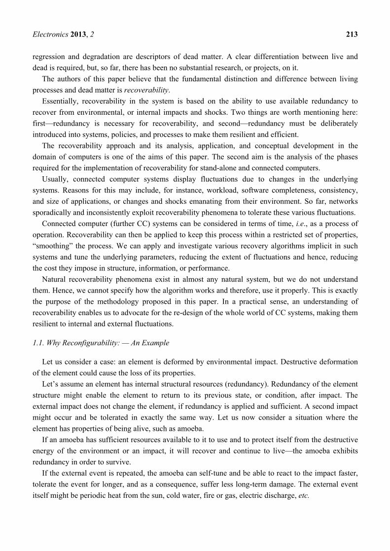
of recovery, or both increase. A sequence of impacts and element recovery is presented in Figure 1.

Figure 1. Periodic impacts, element’s time to recover.

Periodic impacts

Recovery Recovery Recovery

The circles show the state of an element over time, where green indicates an element in a good, or

acceptable steady state and red indicates an element under recovery. Figure 1 indicates an element that

adapts to the periodic external stimulus, can decrease the time for its recovery.

Where the element may be considered alive, such as in the case of the amoeba, using redundancy

for recovery can reduce the time it takes to react to the same event, provided the event is periodic.

Thus, life might be defined as the following:

An element is called alive, if in repeatable conditions, it is able to recover progressively,

using internal redundancy actively.

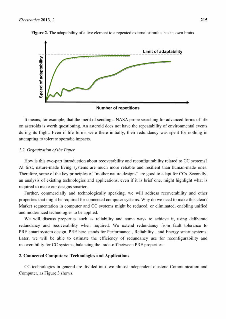
The adaptability of the live element has its limits. Figure 2 shows, for example, an element

approaching the limit of its adaptability and the role of its ability to recover. Whilst wildlife evolution

may be seen as similar to the lower curve, the evolution of “smart” species should be smoother and

faster to reach the same, or higher, limit of adaptability—the shortened curve in the diagram.

Thus, our design of information processing systems, computers, especially complex systems such as

connected computers, can be measured in terms of efficiency of recovery/resilience in comparison

with wildlife phenomena, where available redundancy is used and adaptability grows. In other words,

how good we are at designing our systems to be adaptable can be checked against living objects.

What is the point of this? Without external repeatability of events, evolution is hardly possible;

having internal redundancy to recover is not enough. Evolution depends on the repetition of the same

external events—i.e., no repetition, no evolution.


Figure 2. The adaptability of a live element to a repeated external stimulus has its own limits.

Sp

ee

d o

f a

da

pta

bili

ty

Number of repetitions

Limit of adaptability

It means, for example, that the merit of sending a NASA probe searching for advanced forms of life

on asteroids is worth questioning. An asteroid does not have the repeatability of environmental events

during its flight. Even if life forms were there initially, their redundancy was spent for nothing in

attempting to tolerate sporadic impacts.

1.2. Organization of the Paper

How is this two-part introduction about recoverability and reconfigurability related to CC systems?

At first, nature-made living systems are much more reliable and resilient than human-made ones.

Therefore, some of the key principles of “mother nature designs” are good to adapt for CCs. Secondly,

an analysis of existing technologies and applications, even if it is brief one, might highlight what is

required to make our designs smarter.

Further, commercially and technologically speaking, we will address recoverability and other

properties that might be required for connected computer systems. Why do we need to make this clear?

Market segmentation in computer and CC systems might be reduced, or eliminated, enabling unified

and modernized technologies to be applied.

We will discuss properties such as reliability and some ways to achieve it, using deliberate

redundancy and recoverability when required. We extend redundancy from fault tolerance to

PRE-smart system design. PRE here stands for Performance-, Reliability-, and Energy-smart systems.

Later, we will be able to estimate the efficiency of redundancy use for reconfigurability and

recoverability for CC systems, balancing the trade-off between PRE properties.

2. Connected Computers: Technologies and Applications

CC technologies in general are divided into two almost independent clusters: Communication and

Computer, as Figure 3 shows.


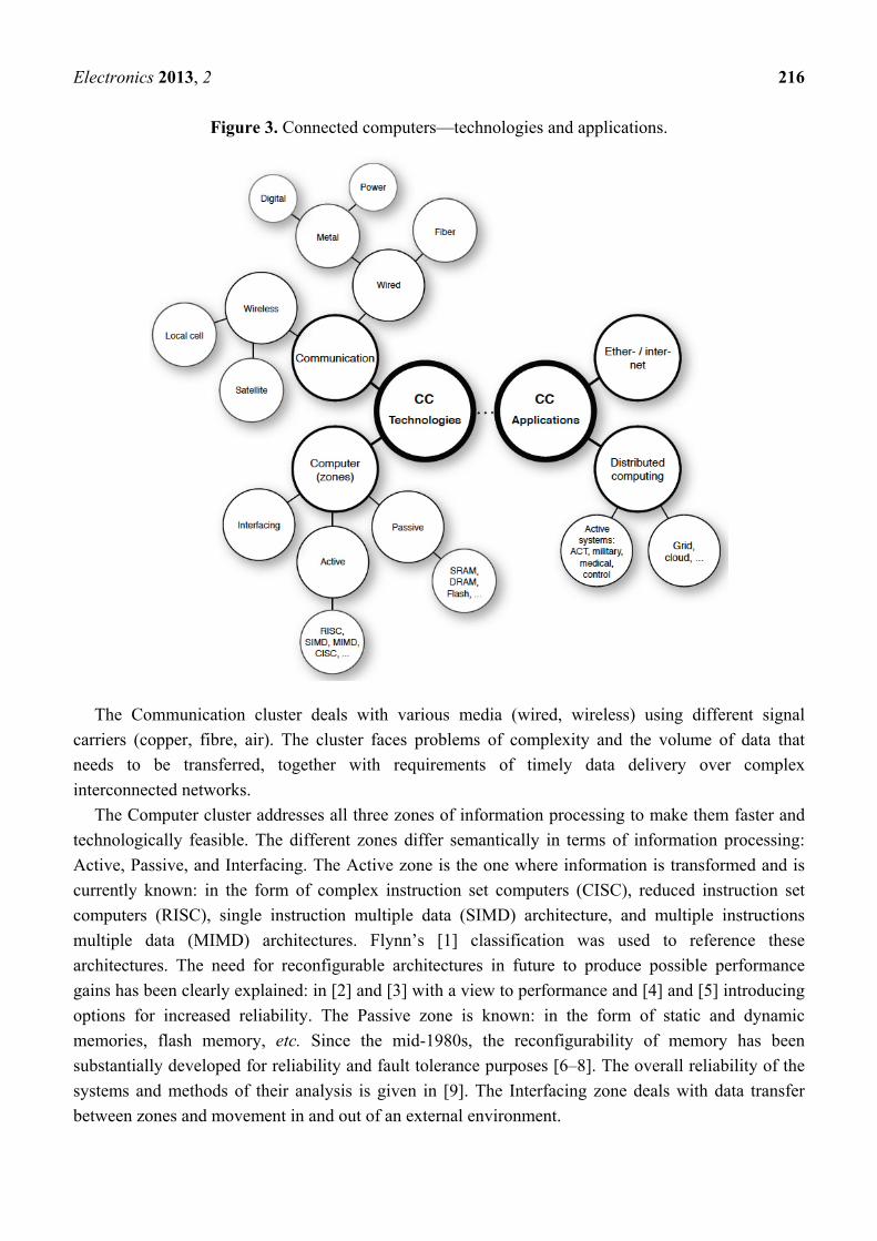
Figure 3. Connected computers—technologies and applications.

The Communication cluster deals with various media (wired, wireless) using different signal

carriers (copper, fibre, air). The cluster faces problems of complexity and the volume of data that

needs to be transferred, together with requirements of timely data delivery over complex

interconnected networks.

The Computer cluster addresses all three zones of information processing to make them faster and

technologically feasible. The different zones differ semantically in terms of information processing:

Active, Passive, and Interfacing. The Active zone is the one where information is transformed and is

currently known: in the form of complex instruction set computers (CISC), reduced instruction set

computers (RISC), single instruction multiple data (SIMD) architecture, and multiple instructions

multiple data (MIMD) architectures. Flynn’s [1] classification was used to reference these

architectures. The need for reconfigurable architectures in future to produce possible performance

gains has been clearly explained: in [2] and [3] with a view to performance and [4] and [5] introducing

options for increased reliability. The Passive zone is known: in the form of static and dynamic

memories, flash memory, etc. Since the mid-1980s, the reconfigurability of memory has been

substantially developed for reliability and fault tolerance purposes [6–8]. The overall reliability of the

systems and methods of their analysis is given in [9]. The Interfacing zone deals with data transfer

between zones and movement in and out of an external environment.


Historically, computer systems were not really fit for the purpose of working within CC systems,

which reduces our expectations when addressing the aspect of distributed computing by design.

Attempts, such as a transputer, also prove that introducing distributiveness into CC is challenging and

not an easy task. CC systems such as the Internet and Ethernet are expanding enormously in terms of

data transfer, video, audio, and e-mails and are moving in a strange direction, allowing home-makers,

young people, financial sector operatives, and bureaucrats communicate and “deliver their messages

and instructions”.

All of the aforementioned applications are not critical in terms of real-time operation; VOIP

requires some traffic shaping to deliver packages with time and other constraints, known as Quality of

Service. This is what the vast majority of CC systems are using. At the moment, according to various

sources, around two billion IP addresses are allocated permanently. This prodigious amount of data

requires handling procedures that need to be much more effective, as everyday life becomes dependent

on the “health” of CC systems. There is a visible shift in the distributed computing paradigm (using

distributed, connected computers to solve large-scale tasks), toward distributed databases, financial

services such as ATM, and so-called “cloud computing”. Putting scepticism aside and leaving other

papers and researchers to discuss what is the real technological progress of cloud computing, we note

here only that the efficiency of large-scale applications, including cloud computing, depends on the

algorithmic skeleton—graphs of data, control and address dependencies [2] and their use, in order to

prepare flexible, reconfigurable and resource-efficient algorithms for distributed computing.

To be effective, distributed computing requires a periodic “tuning” of the CC topology and

computers as the elements in that topology. These tunings of application software, system software,

topology, and internal structure of the computers should be handled statically, before execution and

supported dynamically, during execution.

So far, there has been no visible progress in this direction, in spite of substantial investment under

the flag of cloud computing. At the same time, there is a segment of human life that really requires

attention and the involvement of CC: safety-critical, real-time active control systems, military

applications, health monitoring, etc. All these applications should benefit from CC, but they require the

integrity of a CC system, in terms of hardware, system and application software, user and system data,

and the billions of connected computers to be applied much more efficiently, following the maxima:

Remark 1. Technology must help people to become better, not to be more comfortable.

Therefore, safety critical applications (military, health monitoring, emergency management,

air-traffic control, traffic control at large) should emerge and exploit existing connected computers.

Two approaches to making CC useful are becoming obvious: the application of existing CC to wider

and more challenging areas and the use of specially-built, safety-critical systems for “common”

applications, as a part of the family of CC.

Ignoring any of theses approaches will lead to bigger market clustering and industry segmentation,

resulting in the communication between entities becoming less efficient and which contributes to

increased energy and ecological overheads—an unforgivable waste of resources for human race.


2.1. Problems and Properties

How should we avoid this segmentation in technology and market clustering? Certainly, a CC

system should have some facility to support merging processes, but what are the properties of CC

systems that should be avoided? In addition to the requirement for trustworthy CCs (security of

hardware, system and application software, and user data), widening CC adoption in terms of

application use requires the development of recoverability. Recoverability as a property was explained

in the introduction; it requires an implementation of a generalized algorithm of fault tolerance (GAFT).

GAFT was introduced in [5] and has been applied to various memory structures (Passive zone) [6–8]

and processors (Active zone) [4,5,10]. Note also that recoverability is practical, if it is invisible for the

applications of a CC system.

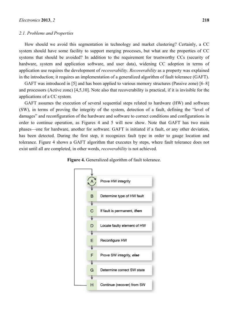
GAFT assumes the execution of several sequential steps related to hardware (HW) and software

(SW), in terms of proving the integrity of the system, detection of a fault, defining the “level of

damages” and reconfiguration of the hardware and software to correct conditions and configurations in

order to continue operation, as Figures 4 and 5 will now show. Note that GAFT has two main

phases—one for hardware, another for software. GAFT is initiated if a fault, or any other deviation,

has been detected. During the first step, it recognizes fault type in order to gauge location and

tolerance. Figure 4 shows a GAFT algorithm that executes by steps, where fault tolerance does not

exist until all are completed, in other words, recoverability is not achieved.

Figure 4. Generalized algorithm of fault tolerance.


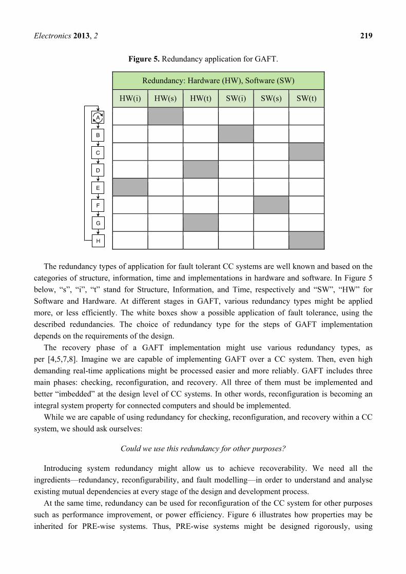
Figure 5. Redundancy application for GAFT.

The redundancy types of application for fault tolerant CC systems are well known and based on the

categories of structure, information, time and implementations in hardware and software. In Figure 5

below, “s”, “i”, “t” stand for Structure, Information, and Time, respectively and “SW”, “HW” for

Software and Hardware. At different stages in GAFT, various redundancy types might be applied

more, or less efficiently. The white boxes show a possible application of fault tolerance, using the

described redundancies. The choice of redundancy type for the steps of GAFT implementation

depends on the requirements of the design.

The recovery phase of a GAFT implementation might use various redundancy types, as

per [4,5,7,8]. Imagine we are capable of implementing GAFT over a CC system. Then, even high

demanding real-time applications might be processed easier and more reliably. GAFT includes three

main phases: checking, reconfiguration, and recovery. All three of them must be implemented and

better “imbedded” at the design level of CC systems. In other words, reconfiguration is becoming an

integral system property for connected computers and should be implemented.

While we are capable of using redundancy for checking, reconfiguration, and recovery within a CC

system, we should ask ourselves:

Could we use this redundancy for other purposes?

Introducing system redundancy might allow us to achieve recoverability. We need all the

ingredients—redundancy, reconfigurability, and fault modelling—in order to understand and analyse

existing mutual dependencies at every stage of the design and development process.

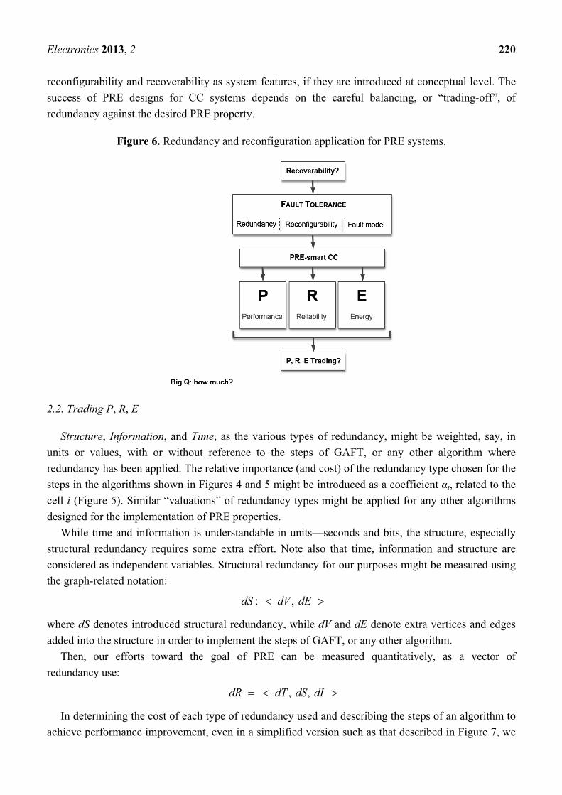
At the same time, redundancy can be used for reconfiguration of the CC system for other purposes

such as performance improvement, or power efficiency. Figure 6 illustrates how properties may be

inherited for PRE-wise systems. Thus, PRE-wise systems might be designed rigorously, using

Redundancy: Hardware (HW), Software (SW)

HW(i) HW(s) HW(t) SW(i) SW(s) SW(t)


reconfigurability and recoverability as system features, if they are introduced at conceptual level. The

success of PRE designs for CC systems depends on the careful balancing, or “trading-off”, of

redundancy against the desired PRE property.

Figure 6. Redundancy and reconfiguration application for PRE systems.

2.2. Trading P, R, E

Structure, Information, and Time, as the various types of redundancy, might be weighted, say, in

units or values, with or without reference to the steps of GAFT, or any other algorithm where

redundancy has been applied. The relative importance (and cost) of the redundancy type chosen for the

steps in the algorithms shown in Figures 4 and 5 might be introduced as a coefficient αi, related to the

cell i (Figure 5). Similar “valuations” of redundancy types might be applied for any other algorithms

designed for the implementation of PRE properties.

While time and information is understandable in units—seconds and bits, the structure, especially

structural redundancy requires some extra effort. Note also that time, information and structure are

considered as independent variables. Structural redundancy for our purposes might be measured using

the graph-related notation:

dS : dV , dE

where dS denotes introduced structural redundancy, while dV and dE denote extra vertices and edges

added into the structure in order to implement the steps of GAFT, or any other algorithm.

Then, our efforts toward the goal of PRE can be measured quantitatively, as a vector of

redundancy use:

dR dT , dS, dI

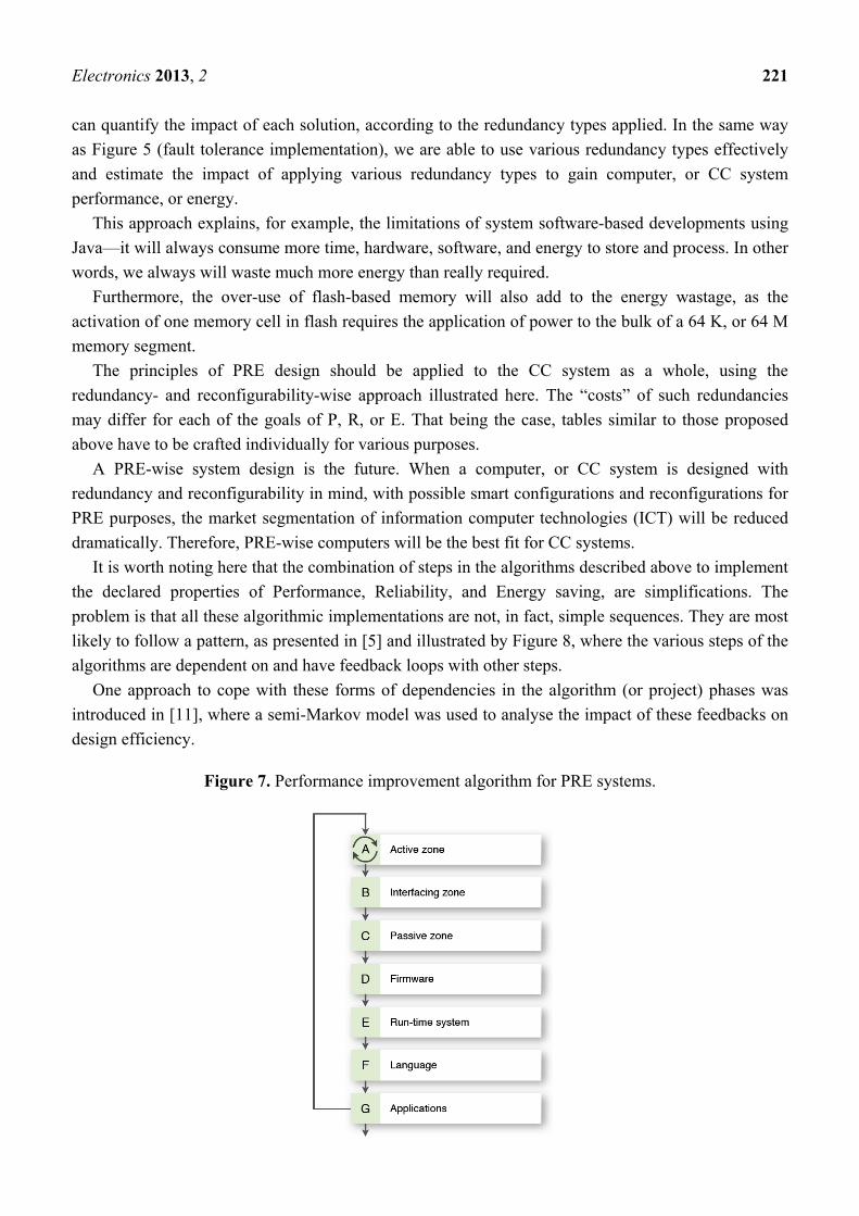
In determining the cost of each type of redundancy used and describing the steps of an algorithm to

achieve performance improvement, even in a simplified version such as that described in Figure 7, we


can quantify the impact of each solution, according to the redundancy types applied. In the same way

as Figure 5 (fault tolerance implementation), we are able to use various redundancy types effectively

and estimate the impact of applying various redundancy types to gain computer, or CC system

performance, or energy.

This approach explains, for example, the limitations of system software-based developments using

Java—it will always consume more time, hardware, software, and energy to store and process. In other

words, we always will waste much more energy than really required.

Furthermore, the over-use of flash-based memory will also add to the energy wastage, as the

activation of one memory cell in flash requires the application of power to the bulk of a 64 K, or 64 M

memory segment.

The principles of PRE design should be applied to the CC system as a whole, using the

redundancy- and reconfigurability-wise approach illustrated here. The “costs” of such redundancies

may differ for each of the goals of P, R, or E. That being the case, tables similar to those proposed

above have to be crafted individually for various purposes.

A PRE-wise system design is the future. When a computer, or CC system is designed with

redundancy and reconfigurability in mind, with possible smart configurations and reconfigurations for

PRE purposes, the market segmentation of information computer technologies (ICT) will be reduced

dramatically. Therefore, PRE-wise computers will be the best fit for CC systems.

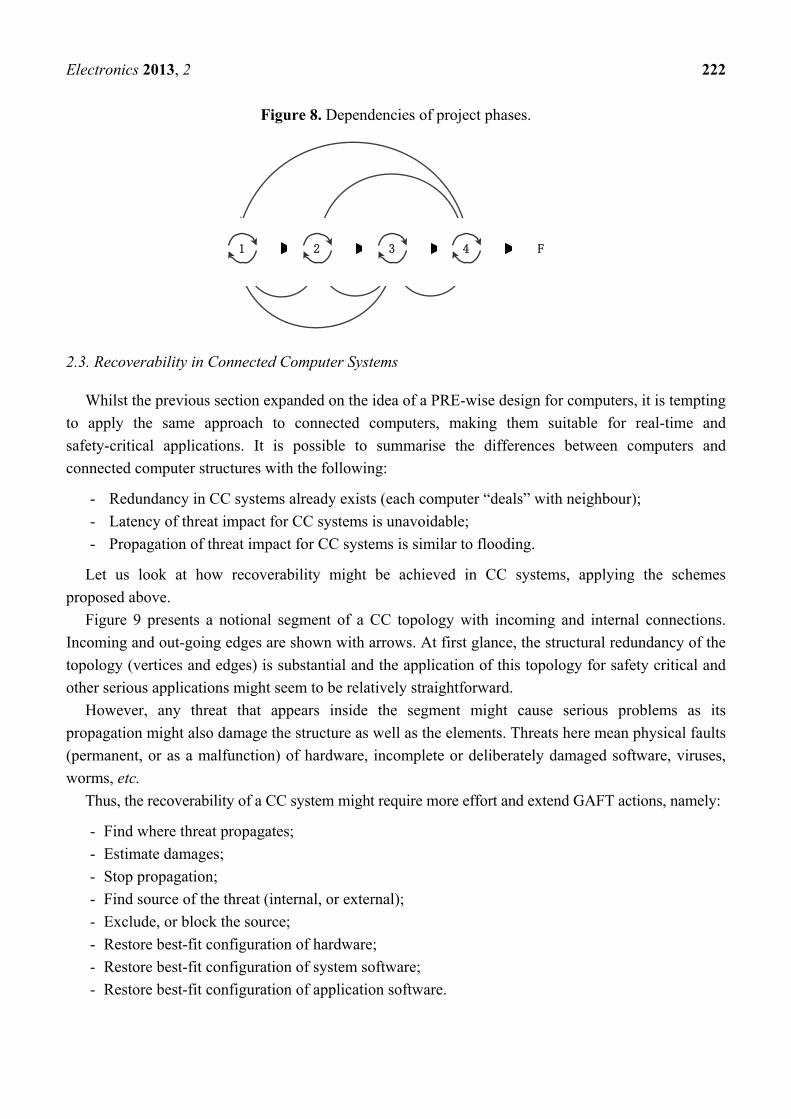
It is worth noting here that the combination of steps in the algorithms described above to implement

the declared properties of Performance, Reliability, and Energy saving, are simplifications. The

problem is that all these algorithmic implementations are not, in fact, simple sequences. They are most

likely to follow a pattern, as presented in [5] and illustrated by Figure 8, where the various steps of the

algorithms are dependent on and have feedback loops with other steps.

One approach to cope with these forms of dependencies in the algorithm (or project) phases was

introduced in [11], where a semi-Markov model was used to analyse the impact of these feedbacks on

design efficiency.

Figure 7. Performance improvement algorithm for PRE systems.


Figure 8. Dependencies of project phases.

1 2 3 4 F

2.3. Recoverability in Connected Computer Systems

Whilst the previous section expanded on the idea of a PRE-wise design for computers, it is tempting

to apply the same approach to connected computers, making them suitable for real-time and

safety-critical applications. It is possible to summarise the differences between computers and

connected computer structures with the following:

- Redundancy in CC systems already exists (each computer “deals” with neighbour);

- Latency of threat impact for CC systems is unavoidable;

- Propagation of threat impact for CC systems is similar to flooding.

Let us look at how recoverability might be achieved in CC systems, applying the schemes

proposed above.

Figure 9 presents a notional segment of a CC topology with incoming and internal connections.

Incoming and out-going edges are shown with arrows. At first glance, the structural redundancy of the

topology (vertices and edges) is substantial and the application of this topology for safety critical and

other serious applications might seem to be relatively straightforward.

However, any threat that appears inside the segment might cause serious problems as its

propagation might also damage the structure as well as the elements. Threats here mean physical faults

(permanent, or as a malfunction) of hardware, incomplete or deliberately damaged software, viruses,

worms, etc.

Thus, the recoverability of a CC system might require more effort and extend GAFT actions, namely:

- Find where threat propagates; - Estimate damages; - Stop propagation; - Find source of the threat (internal, or external); - Exclude, or block the source; - Restore best-fit configuration of hardware; - Restore best-fit configuration of system software; - Restore best-fit configuration of application software.


To make a system of CC useful for real-time applications, one has to introduce exactly the same

procedures that form GAFT (Figure 4) and do a little bit extra: analyse the possible damages, together

with an estimation of the potential consequences for the topology of the CC, as well as its elements.

The speed of propagation of a threat through the topology is a factor that defines the requirements for

recovery. In addition, different segments in the topology might have dramatically different importance

for the CC as a whole; for example, compare a gateway host with a simple internal router.

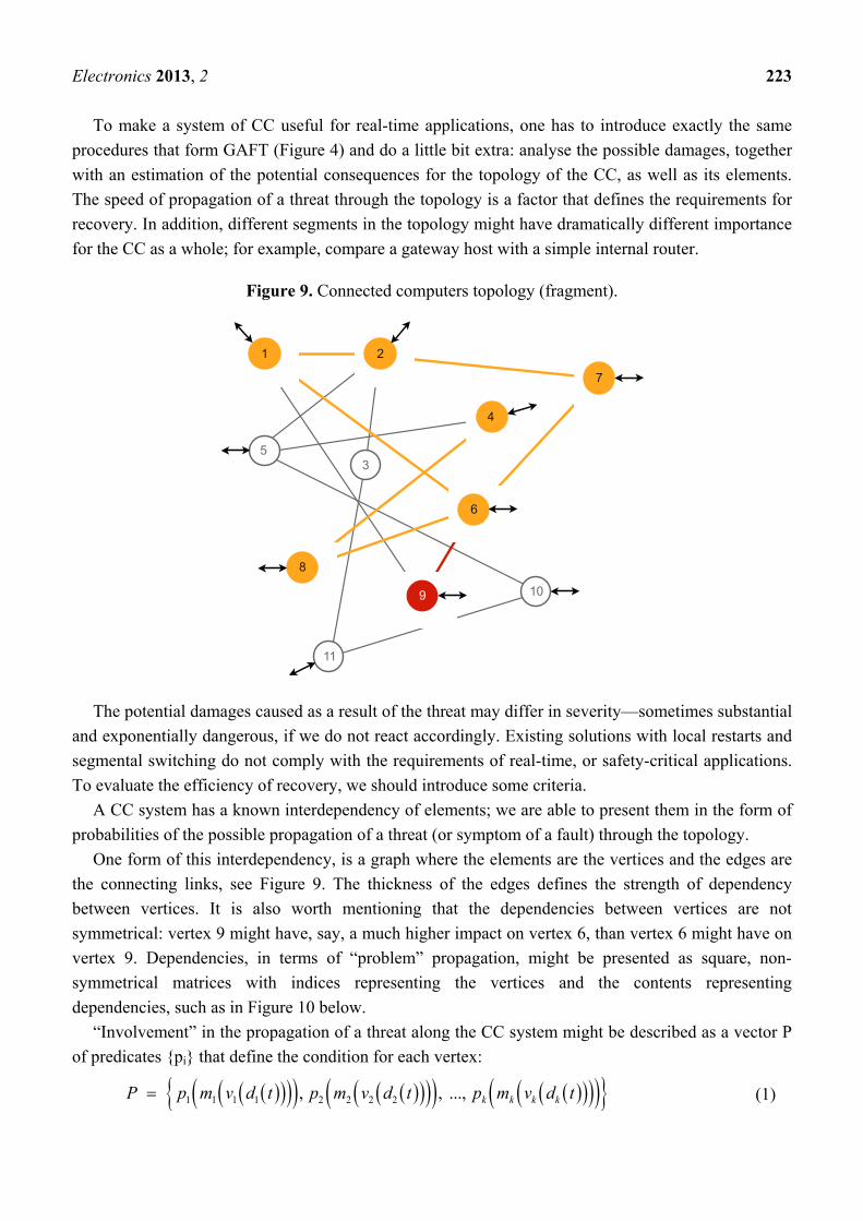
Figure 9. Connected computers topology (fragment).

1 2

4

5

8

11

10

6

7

3

9

The potential damages caused as a result of the threat may differ in severity—sometimes substantial

and exponentially dangerous, if we do not react accordingly. Existing solutions with local restarts and

segmental switching do not comply with the requirements of real-time, or safety-critical applications.

To evaluate the efficiency of recovery, we should introduce some criteria.

A CC system has a known interdependency of elements; we are able to present them in the form of

probabilities of the possible propagation of a threat (or symptom of a fault) through the topology.

One form of this interdependency, is a graph where the elements are the vertices and the edges are

the connecting links, see Figure 9. The thickness of the edges defines the strength of dependency

between vertices. It is also worth mentioning that the dependencies between vertices are not

symmetrical: vertex 9 might have, say, a much higher impact on vertex 6, than vertex 6 might have on

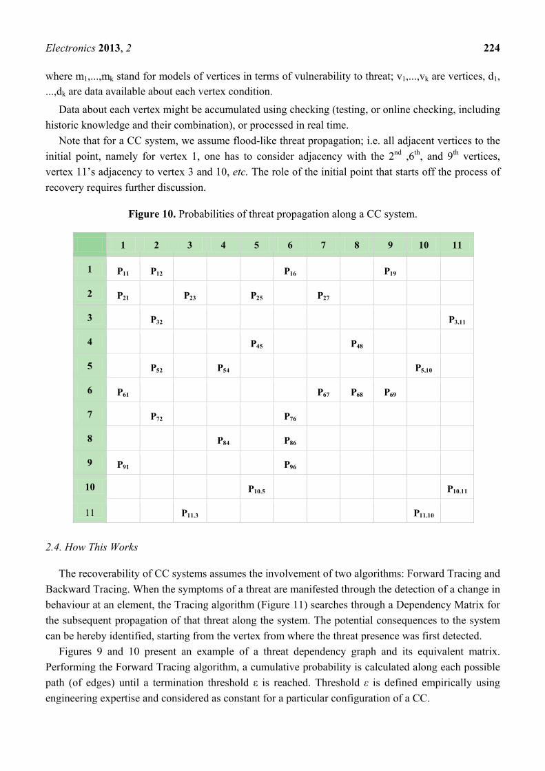
vertex 9. Dependencies, in terms of “problem” propagation, might be presented as square, non-

symmetrical matrices with indices representing the vertices and the contents representing

dependencies, such as in Figure 10 below.

“Involvement” in the propagation of a threat along the CC system might be described as a vector P

of predicates {pi} that define the condition for each vertex:

P p1 m1 v1 d1 t , p2 m2 v2 d2 t , ..., pk mk vk dk t (1)


where m1,...,mk stand for models of vertices in terms of vulnerability to threat; v1,...,vk are vertices, d1, ...,dk are data available about each vertex condition.

Data about each vertex might be accumulated using checking (testing, or online checking, including

historic knowledge and their combination), or processed in real time.

Note that for a CC system, we assume flood-like threat propagation; i.e. all adjacent vertices to the

initial point, namely for vertex 1, one has to consider adjacency with the 2nd ,6th, and 9th vertices,

vertex 11’s adjacency to vertex 3 and 10, etc. The role of the initial point that starts off the process of

recovery requires further discussion.

Figure 10. Probabilities of threat propagation along a CC system.

1 2 3 4 5 6 7 8 9 10 11

1 P11 P12 P16 P19

2 P21 P23 P25 P27

3 P32 P3,11

4 P45 P48

5 P52 P54 P5,10

6 P61 P67 P68 P69

7 P72 P76

8 P84 P86

9 P91 P96

10 P10,5 P10,11

11 P11,3 P11,10

2.4. How This Works

The recoverability of CC systems assumes the involvement of two algorithms: Forward Tracing and

Backward Tracing. When the symptoms of a threat are manifested through the detection of a change in

behaviour at an element, the Tracing algorithm (Figure 11) searches through a Dependency Matrix for

the subsequent propagation of that threat along the system. The potential consequences to the system

can be hereby identified, starting from the vertex from where the threat presence was first detected.

Figures 9 and 10 present an example of a threat dependency graph and its equivalent matrix.

Performing the Forward Tracing algorithm, a cumulative probability is calculated along each possible

path (of edges) until a termination threshold ε is reached. Threshold ε is defined empirically using

engineering expertise and considered as constant for a particular configuration of a CC.


Another termination condition for searching the path of threat propagation is obvious—checking all

dependent vertices. When all elements have been traced, one can fully guarantee 100% threat checking

coverage. Unfortunately, this termination condition might not be feasible, as it becomes

scale-dependent on CC system size.

Note here that the probabilistic matrix in Figure 10 is not Markovian, because the sum of

probabilities on the edges at each node may not be equal to 1; in contrast, several edges of a single

node may have significant probabilities.

Figure 11. Forward tracing of possible consequences.


2.5. Probability Along the Path

In the tracing algorithm, the cumulative probability of threat propagation from one element (vertex)

to another along the edges from the suspected node i to node j (possibly via a series of other nodes), is

defined as Π(pi,j).

When several paths lead from node di to node dj, all possible Π(pi,j) are ranked and nodes along the

paths are included into the set of suspected nodes. This algorithm, called Forward Tracing, is shown in

Figure 11.

Starting from the vertex, i, that manifests the threat, its impact is evaluated by searching from d1 to

all directly, or indirectly connected nodes (elements). The result of this search is a ranked list of the

nodes most likely to be affected - the “consequence” of threat propagation. As the threat paths from

each node are evaluated, only the edge with the highest probability is followed at each node. At most,

each node is only ever included once in any path to ensure termination in a graph which

contains loops.

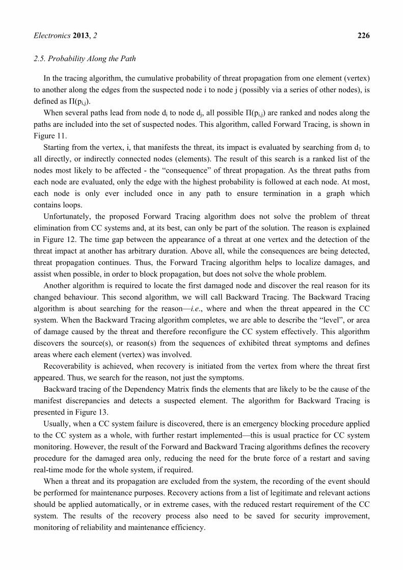
Unfortunately, the proposed Forward Tracing algorithm does not solve the problem of threat

elimination from CC systems and, at its best, can only be part of the solution. The reason is explained

in Figure 12. The time gap between the appearance of a threat at one vertex and the detection of the

threat impact at another has arbitrary duration. Above all, while the consequences are being detected,

threat propagation continues. Thus, the Forward Tracing algorithm helps to localize damages, and

assist when possible, in order to block propagation, but does not solve the whole problem.

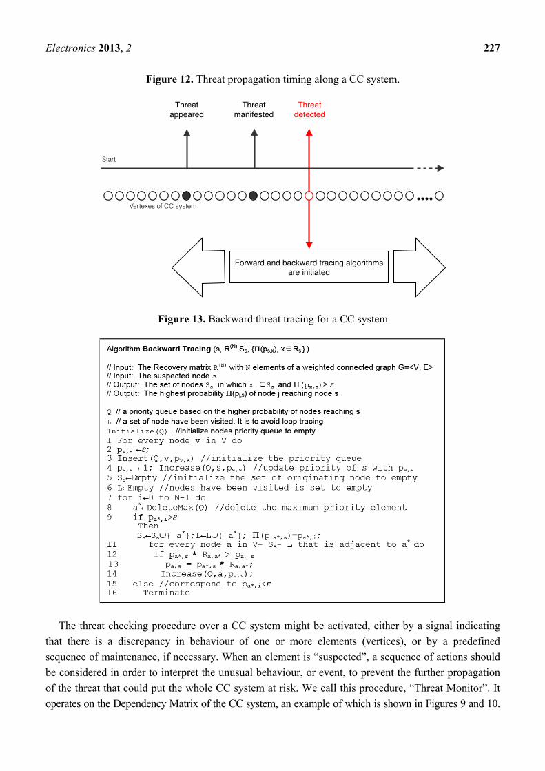
Another algorithm is required to locate the first damaged node and discover the real reason for its

changed behaviour. This second algorithm, we will call Backward Tracing. The Backward Tracing

algorithm is about searching for the reason—i.e., where and when the threat appeared in the CC

system. When the Backward Tracing algorithm completes, we are able to describe the “level”, or area

of damage caused by the threat and therefore reconfigure the CC system effectively. This algorithm

discovers the source(s), or reason(s) from the sequences of exhibited threat symptoms and defines

areas where each element (vertex) was involved.

Recoverability is achieved, when recovery is initiated from the vertex from where the threat first

appeared. Thus, we search for the reason, not just the symptoms.

Backward tracing of the Dependency Matrix finds the elements that are likely to be the cause of the

manifest discrepancies and detects a suspected element. The algorithm for Backward Tracing is

presented in Figure 13.

Usually, when a CC system failure is discovered, there is an emergency blocking procedure applied

to the CC system as a whole, with further restart implemented—this is usual practice for CC system

monitoring. However, the result of the Forward and Backward Tracing algorithms defines the recovery

procedure for the damaged area only, reducing the need for the brute force of a restart and saving

real-time mode for the whole system, if required.

When a threat and its propagation are excluded from the system, the recording of the event should

be performed for maintenance purposes. Recovery actions from a list of legitimate and relevant actions

should be applied automatically, or in extreme cases, with the reduced restart requirement of the CC

system. The results of the recovery process also need to be saved for security improvement,

monitoring of reliability and maintenance efficiency.


Figure 12. Threat propagation timing along a CC system.

Figure 13. Backward threat tracing for a CC system

The threat checking procedure over a CC system might be activated, either by a signal indicating

that there is a discrepancy in behaviour of one or more elements (vertices), or by a predefined

sequence of maintenance, if necessary. When an element is “suspected”, a sequence of actions should

be considered in order to interpret the unusual behaviour, or event, to prevent the further propagation

of the threat that could put the whole CC system at risk. We call this procedure, “Threat Monitor”. It

operates on the Dependency Matrix of the CC system, an example of which is shown in Figures 9 and 10.


For the purpose of maintaining CC system integrity, the procedures for condition checking might be

initiated by choosing any vertex of the CC system at random, or even in a loop covering all vertices.

When a distributed system has Forward Tracing and Backward Tracing algorithms applied to it,

there may be a dynamic and active improvement in reliability and safety [12]. Where recoverability is

implemented, deviations in performance are smoothed out for the system as a whole.

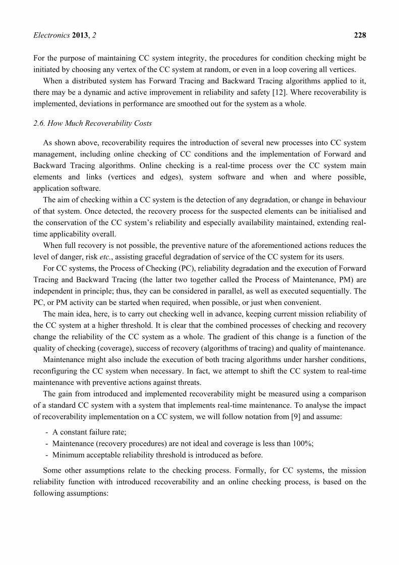
2.6. How Much Recoverability Costs

As shown above, recoverability requires the introduction of several new processes into CC system

management, including online checking of CC conditions and the implementation of Forward and

Backward Tracing algorithms. Online checking is a real-time process over the CC system main

elements and links (vertices and edges), system software and when and where possible,

application software.

The aim of checking within a CC system is the detection of any degradation, or change in behaviour

of that system. Once detected, the recovery process for the suspected elements can be initialised and

the conservation of the CC system’s reliability and especially availability maintained, extending real-

time applicability overall.

When full recovery is not possible, the preventive nature of the aforementioned actions reduces the

level of danger, risk etc., assisting graceful degradation of service of the CC system for its users.

For CC systems, the Process of Checking (PC), reliability degradation and the execution of Forward

Tracing and Backward Tracing (the latter two together called the Process of Maintenance, PM) are

independent in principle; thus, they can be considered in parallel, as well as executed sequentially. The

PC, or PM activity can be started when required, when possible, or just when convenient.

The main idea, here, is to carry out checking well in advance, keeping current mission reliability of

the CC system at a higher threshold. It is clear that the combined processes of checking and recovery

change the reliability of the CC system as a whole. The gradient of this change is a function of the

quality of checking (coverage), success of recovery (algorithms of tracing) and quality of maintenance.

Maintenance might also include the execution of both tracing algorithms under harsher conditions,

reconfiguring the CC system when necessary. In fact, we attempt to shift the CC system to real-time

maintenance with preventive actions against threats.

The gain from introduced and implemented recoverability might be measured using a comparison

of a standard CC system with a system that implements real-time maintenance. To analyse the impact

of recoverability implementation on a CC system, we will follow notation from [9] and assume:

- A constant failure rate;

- Maintenance (recovery procedures) are not ideal and coverage is less than 100%;

- Minimum acceptable reliability threshold is introduced as before.

Some other assumptions relate to the checking process. Formally, for CC systems, the mission

reliability function with introduced recoverability and an online checking process, is based on the

following assumptions:


Assumption 1: Coverage is not 100%. Coverage percentage is 100α%, where 0 < α < 1, and is

assumed to be constant over all preventive maintenance actions. Assumption 2: Preventive maintenance is instantaneous and doesn’t delay the CC system. Assumption 3: A threshold, MR0, of acceptable mission reliability is given (fixed). Assumption 4: TPM is not a constant, but a variable, actually a function of several variables,

including α, λ and MR0.

Mission reliability for a CC system can then be calculated as:

MR(t) ne (t TPM (i ))

i0

n

, TPM (i ) t

i1

n

MR( TPM (i)) MR0i1

n

(2)

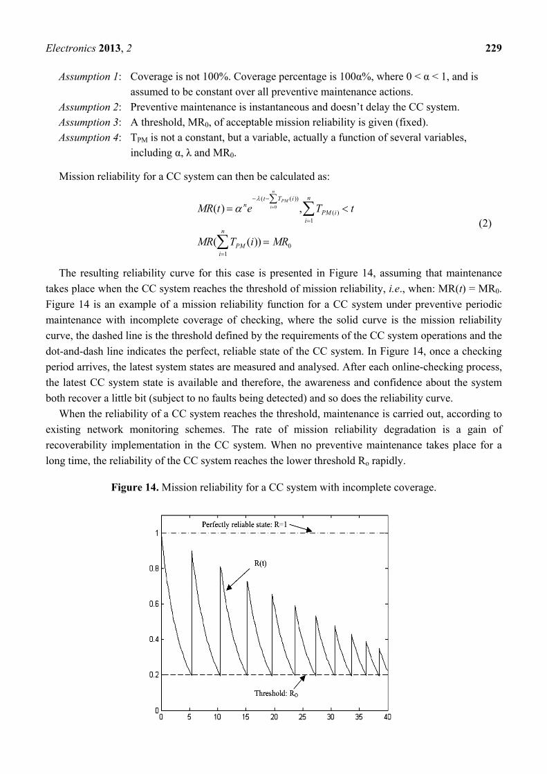
The resulting reliability curve for this case is presented in Figure 14, assuming that maintenance

takes place when the CC system reaches the threshold of mission reliability, i.e., when: MR(t) = MR0.

Figure 14 is an example of a mission reliability function for a CC system under preventive periodic

maintenance with incomplete coverage of checking, where the solid curve is the mission reliability

curve, the dashed line is the threshold defined by the requirements of the CC system operations and the

dot-and-dash line indicates the perfect, reliable state of the CC system. In Figure 14, once a checking

period arrives, the latest system states are measured and analysed. After each online-checking process,

the latest CC system state is available and therefore, the awareness and confidence about the system

both recover a little bit (subject to no faults being detected) and so does the reliability curve.

When the reliability of a CC system reaches the threshold, maintenance is carried out, according to

existing network monitoring schemes. The rate of mission reliability degradation is a gain of

recoverability implementation in the CC system. When no preventive maintenance takes place for a

long time, the reliability of the CC system reaches the lower threshold Ro rapidly.

Figure 14. Mission reliability for a CC system with incomplete coverage.


2.7. Recoverability Implementation Using Online Checking and Recovery

As mentioned already, real-time online checking and recovery should be introduced into the process

of CC system monitoring. Online checking is a process of real-time checking of the system’s main

elements, including hardware (the vertices and edges in Figure 9) and software. The aim of checking is

the detection of degradation, or change in behaviour. If and when possible, it also includes the

recovery of the suspected element(s) and therefore, the conservation of the system’s mission reliability

and availability.

As above, the main idea here is to carry out checking well in advance, providing the CC system

with the highest mission reliability in real time. The introduction of a mission reliability function for a

CC system, with an assumption of real-time maintenance (online checking and recovery actions),

needs some assumptions as well:

Assumption 1: Coverage of real-time maintenance is limited. Coverage is αM100%, where,

0 < αM < 1, and αM is assumed a constant.

Assumption 2: Threshold for mission reliability, or availability MR0 exists for MR(t)

Assumption 3: Online checking process with period TPC is introduced. TPC is a constant.

Assumption 4: After each online checking, the confidence about a CC system’s condition is

increased, therefore MR(t) grows as αC100%, while 0 < αC < 1 and αC is a constant.

Assumption 5: The period between two successive inspections is TPM(i). TPM(i) is a variable,

actually a function of i, R0, αC, αM, λ and TPC.

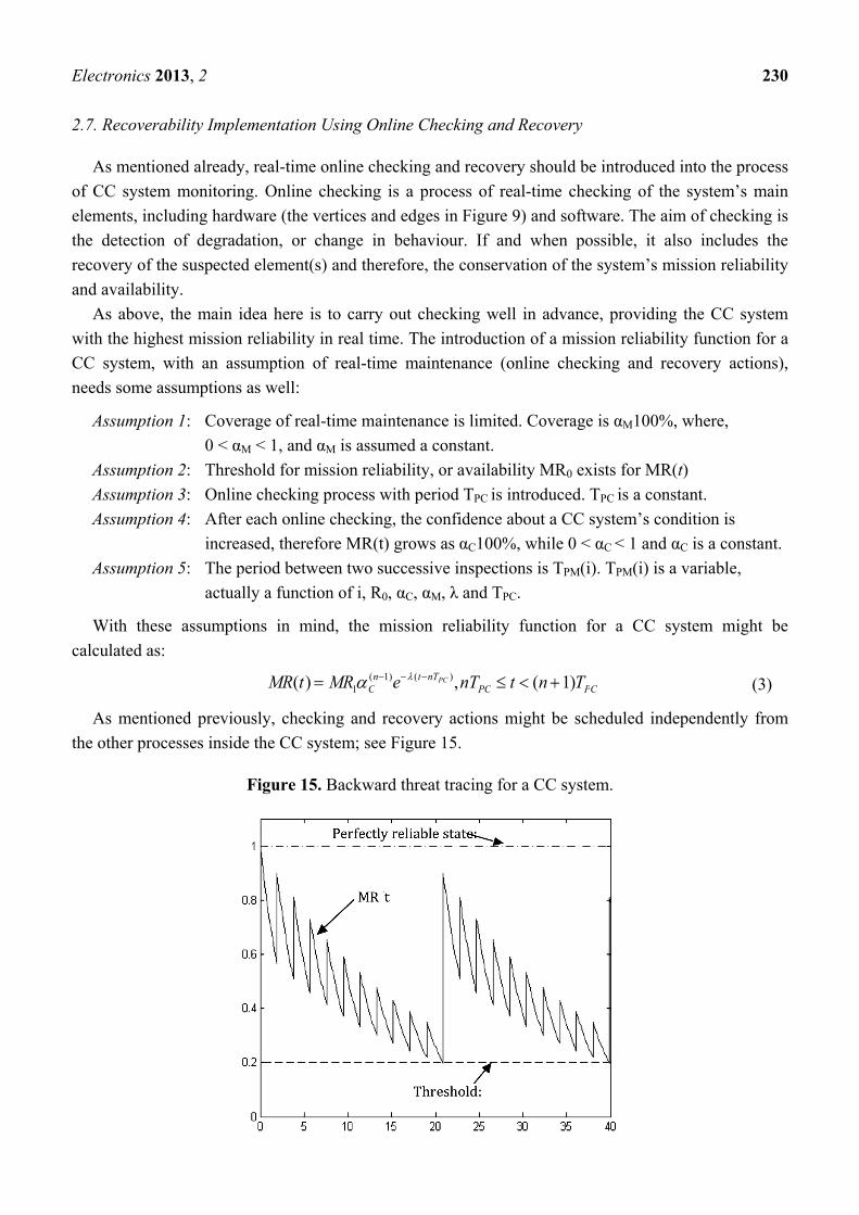
With these assumptions in mind, the mission reliability function for a CC system might be

calculated as:

MR(t) MR1C(n1)e (tnTPC ),nTPC t (n 1)TPC (3)

As mentioned previously, checking and recovery actions might be scheduled independently from

the other processes inside the CC system; see Figure 15.

Figure 15. Backward threat tracing for a CC system.


Comparisons of the lifespan of a CC system under a known maintenance strategy, as well as under

the proposed new scheme, can be executed using integration of reliability over a given time period.

In practice, this means the volume of the area bounded by the mission reliability curve and the

reference axes. The main reason for this index is to show how reliable a CC system is during a given

period of time.

The integration values of mission reliability under conditional maintenance and preventive

maintenance are calculated by Equations 4 and 5, respectively:

VCM (T1) MRCM (t)dt0

T1

, (4)

VPM (T2 ) MRPM (t)dt0

T2

(5)

where MRCM and MRPM are given by Equations 2 and 3.

The efficiency of the preventive over conditional maintenance, can be assessed as:

y(T1,T2 ) VPM (T2 )VCM (T1)

VCM (T1) (6)

assuming T1 = T2 in order to compare the reliability of CC systems with implemented conditional maintenance and preventive maintenance (and recovery), within the same period of time.

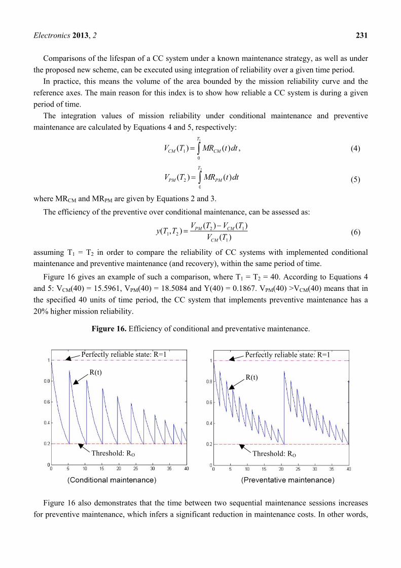
Figure 16 gives an example of such a comparison, where T1 = T2 = 40. According to Equations 4

and 5: VCM(40) = 15.5961, VPM(40) = 18.5084 and Y(40) = 0.1867. VPM(40) >VCM(40) means that in

the specified 40 units of time period, the CC system that implements preventive maintenance has a

20% higher mission reliability.

Figure 16. Efficiency of conditional and preventative maintenance.

Perfectly reliable state: R=1 Perfectly reliable state: R=1

Threshold: RO

R(t)

Threshold: RO

R(t)

Figure 16 also demonstrates that the time between two sequential maintenance sessions increases

for preventive maintenance, which infers a significant reduction in maintenance costs. In other words,


recoverability, implemented as described in this paper, substantially extends the resilience of a CC

system, improving its performance for real-time applications.

3. Conclusions and Future Work

- Recoverability supported by redundancy and reconfigurability is introduced and analysed for

computer systems and connected computer systems.

- A design concept of PRE-wise (Performance-, Reliability- and Energy-wise) systems is proposed

as a unified approach. Computer technologies are analysed in terms of implementation and

recoverability as a fundamental property and in terms of an implementation process using

Forward Tracing and Backward Tracing algorithms.

- It is shown that recoverability makes computers and connected computer systems operational in

a wider market domain, approaching real-time and safety-critical applications.

- An impact of recoverability on mission reliability is proposed, including integrated estimation.

- It is shown that real-time monitoring of a system’s condition with evaluation of possible

damages, supported with knowledge of the localised area of threat propagation, makes

substantial improvements to the integrated reliability characteristics.

- As a future development, it is suggested that the development of a PRE framework, assuming

mutual dependencies of phases of design, is put forward using a semi-Markov model.

Conflicts of Interest

The authors declare no conflict of interest.

References

1. Flynn, M. Some computer organizations and their effectiveness. IEEE Trans. Comput. 1972,

C-21, 948.

2. Tredennik, N.; Shimamoto, B. Inevitability of reconfigurable systems. Queue 2003, 1, 35–43.

3. Goldstein, S.C.; Schmit, H.; Budiu, M.; Cadambi, S.; Moe, M.; Taylor, R.R. PipeRench: A

reconfigurable architecture and compiler. IEEE Comput. 2000, 33, 70–77.

4. Schagaev, I.; Stepaniants A. Malfunction Tolerant Ultra Reliable Processor with Reduced

Instruction Set. Annual IEEE/IFIP International Conference on Dependable Systems and

Networks, Goteborg Sweden, July 2001.

5. Schagaev, I. Reliability of Malfunction Tolerance. Proceedings of IMCSIT 2008, pp. 733–738,

ISBN 978-83-60810-14-9. IEEE explore.

6. Buhanova G. High reliability random access memory devices—Tendencies and progress. Autom.

Remote Control J. 1993, 2, 3–28.

7. Bernstein, A.; Yu, L.; Tomfield, Y.L.; Schagaev, I.V. Storage unit with high reliability

characteristics. I. Avtomat. i Telemekh. 1992, 145–152.

8. Buhanova, G.; Schagaev, I. Ultra reliable TRAM and its analysis. Annual IEEE/IFIP International

Conference on Dependable Systems and Networks IEEE/DSN01, Goteborg, Sweden, July 2001.


9. Birolini, A. Reliability Engineering Theory and Practice, 6th ed.; Springer-Verlag: Berlin,

Heidelberg, Germany, 2010.

10. Schagaev, I.; Kaegi, T.; Gutkneht, J. ERA: Evolving Reconfigurable Architecture. In Proceedings

of the 11th ACIS International Conference on Software Engineering, Artificial Intelligences,

Networking and Parallel/Distributed Computing, London, UK, 9–11 June 2010.

11. Plyaskota, S.; Schagaev, I. Economic efficiency of fault tolerance. Autom. Remote Cont. 1995, 7,

131–143.

12. Schagaev, I.; Kirk, B.; Schagaev, A. Method and Apparatus for Active Safety Systems, UK Patent

GB 2448351, INT CL: G05 9/02 (2006.01), Granted 21.09.2011.

© 2013 by the authors; licensee MDPI, Basel, Switzerland. This article is an open access article

distributed under the terms and conditions of the Creative Commons Attribution license

(http://creativecommons.org/licenses/by/3.0/).

Redundancy + Reconfigurability = Recoverability

Documents