Reduction of slow–fast discrete models coupling migration and demography

www.elsevier.com/locate/yjtbi

Author’s Accepted Manuscript

Reduction of slow-fast discrete models couplingmigration and demography

M. Marvá, E. Sánchez, R. Bravo de la Parra, L.Sanz

PII: S0022-5193(08)00366-4DOI: doi:10.1016/j.jtbi.2008.07.014Reference: YJTBI 5218

To appear in: Journal of Theoretical Biology

Received date: 31 January 2008Revised date: 29 May 2008Accepted date: 15 July 2008

Cite this article as: M. Marvá, E. Sánchez, R. Bravo de la Parra and L. Sanz, Reductionof slow-fast discrete models coupling migration and demography, Journal of TheoreticalBiology (2008), doi:10.1016/j.jtbi.2008.07.014

This is a PDF file of an unedited manuscript that has been accepted for publication. Asa service to our customers we are providing this early version of the manuscript. Themanuscript will undergo copyediting, typesetting, and review of the resulting galley proofbefore it is published in its final citable form. Please note that during the production processerrors may be discovered which could affect the content, and all legal disclaimers that applyto the journal pertain.

peer

-005

5450

1, v

ersi

on 1

- 11

Jan

201

1Author manuscript, published in "Journal of Theoretical Biology 258, 3 (2009) 371"

DOI : 10.1016/j.jtbi.2008.07.014

Accep

ted m

anusc

ript

Reduction of Slow-Fast Discrete Models Coupling Migration and

Demography.

M. Marva (1); E. Sanchez (2); R. Bravo de la Parra (3)(1); L. Sanz (2)(1): Dpto. Matematicas, Universidad de Alcala, 28871 Alcala de Henares, Spain

e-mail M. Marva: [email protected] ; e-mail R. Bravo: [email protected](2): Dpto. Matematica Aplicada, E.T.S. Ingenieros Industriales,

C. Jose Gutierrez Abascal 2, 28006 Madrid, Spaine-mail E. Sanchez: [email protected] ; e-mail L. Sanz: [email protected]

(3): UR GEODES, IRD, 32, Avenue Henri Varagnat, 93143 -Bondy cedex, France

Abstract

This work deals with a general class of two-time scales discrete nonlineardynamical systems which are susceptible of being studied by means of a reducedsystem that is obtained using the so-called aggregation of variables method.This reduction process is applied to several models of population dynamicsdriven by demographic and migratory processes which take place at two differenttime scales: slow and fast. An analysis of these models exchanging the role ofthe slow and fast dynamics is provided: when a Leslie type demography is fasterthan migrations, a multi-attractor scenario appears for the reduced dynamics;on the other hand, when the migratory process is faster than demography,the reduction process gives rise to new interpretations of well known discretemodels, including some Allee effect scenarios.

Keywords: Nonlinear discrete models; aggregation of variables; time scales;population dynamics.

AMS Classification: 39A11; 92D25.

1 Introduction.

Ecological models always entail a decision on the level of detail to be included inthem, and this decision should be taken on the basis of optimizing the benefit ofthe study. Any model is a compromise between generality and simplicity on the onehand and biological realism on the other. The more biological details are includedin specifying a model the more complicated and specific it becomes.

Nature offers many examples of systems where several processes act at differenttime scales. It is then usual to consider those events occurring at the fast scaleas being instantaneous with respect to the slower ones. This sort of decouplingimplies a reduction of the number of variables or parameters needed to describethe evolution of the system. A subsequent issue is to determine conditions forthese reductions to give good approximations of the real results. An example of thisgeneral framework are the so-called aggregation methods which study the relationshipbetween a large class of two-time scales complex systems and their correspondingaggregated or reduced ones. The aim of aggregation methods is twofold. On theone hand they construct the reduced systems that summarize the dynamics of thecomplex ones, thus simplifying their analytical study, and on the other hand, lookingat the relationship in the opposite sense, the complex systems serve as explanationsof the simple form of the aggregated ones. A review on these methods in differentmathematical settings, with updated bibliography can be found in [3] and [4].

1

peer

-005

5450

1, v

ersi

on 1

- 11

Jan

201

1

Accep

ted m

anusc

ript

In this work we will apply the aggregation of variables method in the setting ofdiscrete dynamical systems. In the construction of a discrete model with two timescales it is essential to decide if the time unit should be associated to the slow processor to the fast one. The references [7] and [9] study models in which the time unitof the dynamical system is chosen to be that of the fast dynamics. Nevertheless,this choice is not always possible, because the action of the slow process during afast time unit may not be describable. But if the system is expressed in the slowtime unit, it is always possible to describe the action of the fast process during it byrepeating a large enough number of times its action during a slow unit. From thispoint of view, it is interesting to extend to nonlinear cases previous work, made bysome of us, that develop the methods of aggregation of variables for linear discretesystems expressed in the slow time unit (see [15], [16]).

A first attempt to do this is [8], where the slow dynamics is assumed to be linear.An extension to a general class of nonlinear discrete models has been recently madeby some of the authors and can be found in [17]. In this work, a very general discretesystem including two different processes acting at different time scales is proposed.The time unit is the one corresponding to the slow dynamics and the effect of thefast dynamics is represented assuming that the slow time unit is divided into alarge number of fast time units and so that it acts a large number of times duringone single slow time unit. Then some assumptions, generalizing those requiredin previous works, are proposed which allow the construction of a reduced modelassociated to the original one. Several results relating the solutions to both systemshave been established: it is possible to study the existence, stability and basins ofattraction of steady states and periodic solutions to the original system performingthe study for the corresponding aggregated system.

The hypotheses of the general results of [17] are not easy to prove in particularcases. In [12] this is done for a particular multi-patch host-parasitoid model wheremigration, which is fast in comparison to demography, is considered density inde-pendent for hosts and dependent on local host population density for parasitoids.In this work we present a general class of two-time scales nonlinear discrete modelsas a particular case of the more abstract setting described in [17]. Then we con-struct the corresponding reduced models and prove that the approximation resultsestablished in [17] are valid. The reduction process is applied to several modelsof population dynamics driven by nonlinear demographic and migration processeswhich take place at two different time scales, slow and fast. We provide an analysisof these models exchanging the role of the slow and fast dynamics: when a Leslietype demography is faster than migrations, a multi-attractor scenario appears forthe aggregated dynamics; on the other hand, when the migratory process is fasterthan demography, by introducing different migration schemes we derive some wellknown discrete models whose analysis gives rise to some Allee effect scenarios.

The organization of the paper is as follows: In Section 2 we specify the mathe-matical formulation of a general class of two-time scales discrete nonlinear dynamicalsystems to which a reduction process can be applied, yielding the so-called aggregatedmodel, whose dynamical features approximate those of the original more complexmodel. Section 3 is devoted to the application of these mathematical results to sev-eral specific models of population dynamics. Some conclusions are given in Section

2

peer

-005

5450

1, v

ersi

on 1

- 11

Jan

201

1

Accep

ted m

anusc

ript

4. To facilitate the reading, technical mathematical proofs of the results establishedin Section 2 are deferred to a final Appendix.

2 Application of the aggregation of variables method to

the reduction of a general nonlinear discrete dynam-

ical system.

The main goal of this section is to apply the aggregation of variables method to thereduction of a general class of nonlinear discrete models with two time scales, whichfit in the framework of an original formulation made by some of the authors anddeveloped in detail in [17]. To facilitate the reading, we will start describing themodel and its main mathematical features, as done in [17].

First of all, let us present the so-called complete or general system to which theaggregation of variables method will be applied.

The model evolves in discrete time and is driven by two processes with differenttime scales, slow and fast. Such processes are defined respectively by two mappings

S,F : ΩN −→ ΩN , S, F ∈ C1(ΩN )

where ΩN ⊂ RN is a non-empty open set.We choose as time step of the model that corresponding to the slow dynamics. In

order to approximate the effect of the fast process over a time interval much biggerthan its own, we assume that during this time step the fast process acts k timesbefore the slow process acts, where k is a positive integer that in applications willtake a big value.

Therefore, denoting by Xk,n ∈ RN the vector of state variables at time n, thecomplete or general system is defined by

Xk,n+1 = S(F k(Xk,n)

)=: Hk(Xk,n) (1)

where F k denotes the k-fold composition of F with itself.In order to reduce the system (1), we have to impose some conditions on the fast

process, which are specified in the following hypothesis:

Hypothesis 1 For each initial condition X ∈ ΩN , the fast dynamics tends to anequilibrium. That is, there exists a mapping F : ΩN → ΩN , F ∈ C1(ΩN ), such that

∀X ∈ ΩN , limk→∞

F k(X) = F (X).

Moreover, there exist a nonempty open set Ωq ⊂ Rq with q < N , and two mappings

G : ΩN −→ Ωq , G ∈ C1(ΩN ) ; E : Ωq −→ ΩN , E ∈ C1(Ωq)

such that F can be expressed as F = E G.

3

peer

-005

5450

1, v

ersi

on 1

- 11

Jan

201

1

Accep

ted m

anusc

ript

Let us define a new set of variables, called global variables, by

Yn := G(Xn).

The reduced or aggregated system which approximates system (1) is given by

Yn+1 = G S E (Yn) := H(Yn). (2)

Note that through this procedure we have constructed an approximation thatallows us to reduce a system with N variables to a new system with q variables. Inmost practical applications, q will be much smaller than N .

To establish a relationship between the solutions to systems (1) and (2), thefollowing assumption is crucial:

Hypothesis 2 The mappings F and F satisfy that

limk→∞

F k = F ; limk→∞

DF k = DF

uniformly on any compact set K ⊂ ΩN .

As usual, the notation DF represents the differential of F .Then, the following theorem, whose details can be found in [17], guarantees that

the existence of an equilibrium point Y ∗ for the aggregated system implies, for largeenough k, the existence of an equilibrium X∗

k for the original system, which can beapproximated in terms of Y ∗. Moreover, in the hyperbolic case, the stability of Y ∗

is equivalent to the stability of X∗

k and in the asymptotically stable (A.S.) case, thebasin of attraction of X∗

k can be approximated in terms of the basin of attraction ofY ∗.

Theorem 1 Under Hypotheses 1 and 2, let Y ∗ ∈ Rq be a hyperbolic equilibriumpoint of system (2). Then, there exists an integer k0 ≥ 0 such that for all k ≥ k0

system (1) has an equilibrium point X∗

k which is hyperbolic and satisfies

limk→∞

X∗

k = X∗ ; X∗ := S E(Y ∗).

Moreover, the following holds:

i) X∗

k is A.S. (resp. unstable) if and only if Y ∗ is A.S. (resp. unstable).

ii) Let Y ∗ be A.S. and let X0 ∈ ΩN be such that Y0 := G(X0) satisfies thatlimn→∞ H

n(Y0) = Y ∗. Then, for all k ≥ k0, limn→∞ Hn

k (X0) = X∗.

Although it is not stated in Theorem 1, these results are also valid for m-periodicpoints (see [17]).

Let us recall that an equilibrium point X∗ of a discrete dynamical system Xn+1 =T (Xn) is hyperbolic if none of the eigenvalues of the differential operator DT (X∗)has modulus 1. If all the eigenvalues of DT (X∗) have modulus strictly less than 1,then X∗ is A.S. and the set of initial conditions whose corresponding solutions tendto X∗ is called the basin of attraction. If any of the eigenvalues of DT (X∗) havemodulus larger than 1, then X∗ is unstable. See [14] for the general theory.

4

peer

-005

5450

1, v

ersi

on 1

- 11

Jan

201

1

Accep

ted m

anusc

ript

2.1 Fast dynamics depending on global variables.

As we mentioned in the introduction, for a particular two time scales discrete modelit is difficult to prove that Hypothesis 2 in Theorem 1 is met. Here we present aclass of models for which this is proved and so Theorem 1 applies.

Let us suppose a population divided into groups, and each of these groups dividedinto several subgroups. We can think, for instance, of an age-structured populationoccupying a multi-patch environment. In this case, the population can be considereddivided into groups which are the age classes, and each group divided into subgroupswhich are the individuals inhabiting each of the different patches.

The state at time n of a population distributed into q groups is represented by avector Xn := (x1

n, . . . , xqn)T ∈ RN

+ , where each vector xin := (xi1

n , . . . , xiN i

n )T ∈ RN i

+ ,i = 1, . . . , q, represents the state of the i-group which in turn is divided into N i

subgroups with N = N1 + · · · + N q.Following [15], we will suppose that for each group i = 1, . . . , q, the fast dynamics

is internal, conservative of the total number of individuals and with an asymptot-ically stable distribution among the groups. These assumptions are met in theparticular case of representing the fast dynamics for each group i by a projectionmatrix which is a regular stochastic matrix of dimensions N i × N i. Hypothesis 2in Theorem 1 is trivially satisfied if these projection matrices are constant. Ouraim in what follows is to extend this situation to the nonlinear case in which suchprojection matrices depend on the total number of individuals in each group. To beprecise, let us introduce some definitions.

Let 1i := (1, . . . , 1)T ∈ RN i

, i = 1, . . . , q, U := diag (1T1 , . . . ,1T

q ) and Ωq :=UΩN ⊂ Rq.

For each i = 1, . . . , q, let Pi(·) ∈ C1(Ωq) be a matrix function such that for all Y ∈Ωq, Pi(Y ) is a regular stochastic matrix of dimensions N i×N i. As a consequence, 1is an eigenvalue simple and strictly dominant in modulus for Pi(Y ), with associatedright and left eigenvectors vi(Y ), 1i, respectively. The eigenvector vi(Y ) is theasymptotically stable probability distribution, i.e., vi(Y ) ≥ 0 and 1T

i vi(Y ) = 1.The fast dynamics for the whole population is represented by the block diagonal

matrix:∀Y ∈ Ωq , F(Y ) := diag (P1(Y ), . . . , Pq(Y )).

The Perron-Frobenius Theorem applies to each matrix Pi(Y ), so that we have

P i(Y ) := limk→∞

P ki (Y ) = (vi(Y )| . . . |vi(Y )) = vi(Y )1T

i

Introducing the notations

F(Y ) := diag (P 1(Y ), . . . , P q(Y )) ; V(Y ) := diag (v1(Y ), . . . ,vq(Y ))

we also have∀Y ∈ Ωq , F(Y ) = lim

k→∞

Fk(Y ) = V(Y )U .

Finally, the nonlinear model that we are considering is formulated as:

Xk,n+1 = S(Fk(UXk,n)Xk,n

). (3)

5

peer

-005

5450

1, v

ersi

on 1

- 11

Jan

201

1

Accep

ted m

anusc

ript

If we think that the ratio of slow to fast time scale tends to infinity i.e., k → ∞,or in other words, that the fast process is instantaneous in relation to the slowprocess, we can approximate system (3) by the following auxiliary system:

Xn+1 = S(F(UXn)Xn) = S(V(UXn)UXn).

We see that the evolution of this system depends on UXn ∈ Rq, which suggests theglobal variables should be defined by:

Yn := UXn

and therefore the aggregated system of system (3) is

Yn+1 = US(V(Yn)Yn). (4)

We can now establish an approximation result between the solutions to the com-plete system (3) and the aggregated model (4), as a consequence of Theorem 1.

Theorem 2 Let Y ∗ ∈ Rq be a hyperbolic equilibrium point of system (4). Then,there exists an integer k0 ≥ 0 such that for all k ≥ k0 system (3) has an equilibriumpoint X∗

k which is hyperbolic and satisfies

limk→∞

X∗

k = X∗ ; X∗ := S(V(Y ∗)Y ∗).

Moreover, the following holds:

i) X∗

k is A.S. (resp. unstable) if and only if Y ∗ is A.S. (resp. unstable).

ii) Let Y ∗ be A.S. and let X0 ∈ ΩN be such that the solution Ynn=0,1,... to (4)corresponding to the initial data Y0 := UX0 satisfies that limn→∞ Yn = Y ∗.Then, for all k ≥ k0, the solution to (3) Xk,nn=0,1,... with Xk,0 = X0 satisfiesthat limn→∞ Xk,n = X∗

k .

Proof.– See Appendix.In some applications, particularly in ecology, it would be more realistic to have

the fast dynamics dependent on the state variables and not just on the global vari-ables as in Theorem 2. Nevertheless, it does not seem easy to find a proof for thismore general case and specific proofs should be provided for each particular case offast dynamics depending on state variables as it is done in [12]. On the other hand,as we will see in the next section, it is possible to develop interesting applicationskeeping in the framework of Theorem 2.

3 Two-time discrete population dynamics models in-

cluding demography and migrations.

In this section we illustrate the previous results by means of some applications. Webegin treating the case of a population inhabiting a multi-patch environment butwith no further structure, thus the corresponding aggregated model is a scalar dif-ference equation. Then we develop the reduction of a model of an age-structuredpopulation in a multi-patch habitat with the special feature of considering demog-raphy fast in comparison with migration. This last example extends slightly theframework presented in Section 2.1.

6

peer

-005

5450

1, v

ersi

on 1

- 11

Jan

201

1

Accep

ted m

anusc

ript

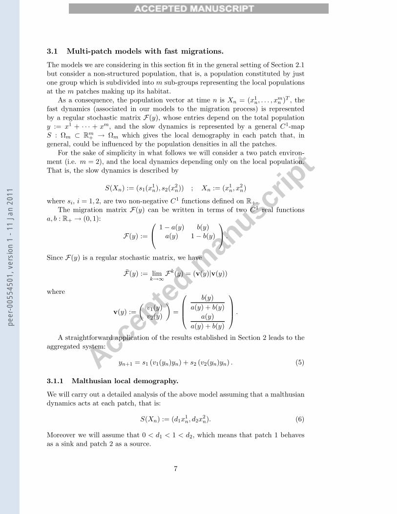
3.1 Multi-patch models with fast migrations.

The models we are considering in this section fit in the general setting of Section 2.1but consider a non-structured population, that is, a population constituted by justone group which is subdivided into m sub-groups representing the local populationsat the m patches making up its habitat.

As a consequence, the population vector at time n is Xn = (x1n, . . . , xm

n )T , thefast dynamics (associated in our models to the migration process) is representedby a regular stochastic matrix F(y), whose entries depend on the total populationy := x1 + · · · + xm, and the slow dynamics is represented by a general C1-mapS : Ωm ⊂ Rm

+ → Ωm which gives the local demography in each patch that, ingeneral, could be influenced by the population densities in all the patches.

For the sake of simplicity in what follows we will consider a two patch environ-ment (i.e. m = 2), and the local dynamics depending only on the local population.That is, the slow dynamics is described by

S(Xn) := (s1(x1n), s2(x

2n)) ; Xn := (x1

n, x2n)

where si, i = 1, 2, are two non-negative C1 functions defined on R+.The migration matrix F(y) can be written in terms of two C1 real functions

a, b : R+ → (0, 1):

F(y) :=

⎛⎝ 1 − a(y) b(y)

a(y) 1 − b(y)

⎞⎠ .

Since F(y) is a regular stochastic matrix, we have

F(y) := limk→∞

Fk(y) = (v(y)|v(y))

where

v(y) :=

(v1(y)v2(y)

)=

⎛⎜⎜⎝

b(y)

a(y) + b(y)

a(y)

a(y) + b(y)

⎞⎟⎟⎠ .

A straightforward application of the results established in Section 2 leads to theaggregated system:

yn+1 = s1 (v1(yn)yn) + s2 (v2(yn)yn) . (5)

3.1.1 Malthusian local demography.

We will carry out a detailed analysis of the above model assuming that a malthusiandynamics acts at each patch, that is:

S(Xn) := (d1x1n, d2x

2n). (6)

Moreover we will assume that 0 < d1 < 1 < d2, which means that patch 1 behavesas a sink and patch 2 as a source.

7

peer

-005

5450

1, v

ersi

on 1

- 11

Jan

201

1

Accep

ted m

anusc

ript

When the slow dynamics is given by (6), the aggregated model (5) reads as:

yn+1 =

(d1b(yn) + d2a(yn)

a(yn) + b(yn)

)yn := h(yn)yn. (7)

It is evident that y0 = 0 is a fixed point of the above model, but we are mainlyinterested in the existence and stability properties of the positive fixed points y∗,which are the solutions to equation h(y) = 1.

To study the behaviour of function h, we should take into account its derivative:

h′(y) = (d2 − d1)a′(y)b(y) − a(y)b′(y)

[a(y) + b(y)]2.

For the sake of simplicity we restrict our analysis to the case in which functions a(y),b(y) are monotone. When one of them is increasing and the other is decreasing, itis evident that h(y) is strictly monotone. Therefore, whether function h(y) crossesor not the line y = 1 is completely determined by the values h(0) and h(∞) :=limy→+∞ h(y). Moreover, in the case in which y∗ exists, it is unique and its stabilityis determined by the value h′(y∗)y∗. On the other hand, the stability of the fixedpoint y0 = 0 depends on the value of h(0).

These results are summarized as follows:

a(y) b(y) h(0) h(∞) y0 = 0 y∗

> 1 ∈ (0, 1) U. ∃, U. or A.S.

> 1 > 1 U.

∈ (0, 1) ∈ (0, 1) G.A.S. ∈ (0, 1) > 1 A.S. ∃, U.

∈ (0, 1) ∈ (0, 1) G.A.S. > 1 > 1 U.

where the arrows and stand for a decreasing and an increasing functionrespectively , and U., A.S. and G.A.S. stand for unstable, asymptotically stable andglobally asymptotically stable, respectively.

The fact that local dynamics are of malthusian type allows extinction and un-bounded growing to be expected at a global level. Nevertheless, as we see in the firstrow of the previous table, certain kinds of density dependent migrations can lead toa positive asymptotically stable equilibrium. Two examples are described below.

If we choose

a(y) =α − d1(1 + βy)

d2 − d1and b(y) =

d2(1 + βy) − α

d2 − d1(8)

for positive parameters α and β, formal calculations yield the well-known Beverton-Holt equation [5]:

yn+1 =αyn

1 + βyn

which always possesses a positive equilibrium whic is globally asymptotically stable.The formal calculations are valid provided that a(y), b(y) ∈ (0, 1), which is true if

α − d2

β< y <

α − d1

d2β.

8

peer

-005

5450

1, v

ersi

on 1

- 11

Jan

201

1

Accep

ted m

anusc

ript

So, if we choose α ∈ (d1, d2) and β ∈ (0, α−d1

d2y ) we can easily prove that a(y), b(y) ∈(0, 1) whenever y ∈ [0, y].

Similar requirements allow us to obtain the Ricker equation [13]

yn+1 = exp(r(1 − yn/K))yn,

where r and K are positive parameters, by choosing

a(y) =er(1−y/K) − d1

d2 − d1and b(y) =

d2 − er(1−y/K)

d2 − d1. (9)

We have illustrated how the aggregation procedure provides an explanation oftwo classical mono-species discrete models in terms of a sink-source environmentwith fast density dependent migrations coupled to simple local malthusian dynamics.Similar approaches using aggregation methods for ordinary differential equationswere presented in [1] and [2].

Some others interpretations of this kind have been recently presented by Geritzand Kisdi ([11]). There, starting from a continuous-time resource-consumer modelfor the dynamics within a year, a discrete-time model for the between-year dynamicsis derived. This model is analyzed assuming that the within-year resource dynamicsin absence of consumers takes different functional forms. Considering particularconstant rates for the influx and efflux of the resource, the Beverton-Holt model,the Ricker model and many other models are recovered. Further models derivedby systematically varying the within year patterns of reproduction and aggressionbetween individuals can be found in [10].

To go on with the study of equation (7), we notice that the cases in which botha(y) and b(y) are simultaneously increasing or decreasing functions yield a morecomplicated dynamics and Allee effect scenarios may arise.

We illustrate this fact with the next example. Let us assume that a(y) and b(y)are increasing functions given by

a(y) :=y2

y2 + βand b(y) :=

y2 + β

y2 + δ, 0 < β < δ.

Function h(y) in (7) becomes

h(y) =d1

(y2 + β

)2+ d2

(y2 + δ

)y2

(y2 + β)2 + (y2 + δ) y2.

The qualitative analysis of equation (7) is straightforward having in mind thatpositive solutions are decreasing if h(y) < 1, increasing if h(y) > 1 and the positivefixed points are the roots of equation h(y) = 1. Since h(0) = d1 < 1, the fixed pointy∗0 = 0 is always asymptotically stable.

To find when h(y) < 1 and when h(y) > 1 we know that h(0) = d1 < 1 andlimy→∞ h(y) = (d1 + d2)/2. Moreover, if we look at the sign of h′(y),

h′(y) =2(d2 − d1)y

((2β − δ)y4 + 2β2y2 + β2δ

)(2y4 + (2β + δ)y2 + β2)2

,

9

peer

-005

5450

1, v

ersi

on 1

- 11

Jan

201

1

Accep

ted m

anusc

ript

we see that if δ ≤ 2β then h(y) is increasing in [0,∞) while if δ > 2β then h(y) isincreasing in [0, yM ) and decreasing in (yM ,∞), where yM =

√βδ/(δ − 2β) is the

only positive root of equation h′(y) = 0. Thus, we have:

• If δ ≤ 2β and (d1 + d2)/2 ≤ 1, there is no positive fixed point.

• If δ ≤ 2β and (d1 +d2)/2 > 1, there is a positive fixed point which is unstable.

• If δ > 2β and h(yM ) < 1, there is no positive fixed point.

• If δ > 2β and h(yM ) = 1, yM is the only positive fixed point and it is unstable.

• If δ > 2β, h(yM ) > 1 and (d1 + d2)/2 ≥ 1, there is a positive fixed point,y∗1 < yM , which is unstable.

• If δ > 2β, h(yM ) > 1 and (d1 + d2)/2 < 1, there are two positive fixed points,y∗1 < yM < y∗2. In this case the positive solutions of equation (7), which are allmonotone, verify the following:

If the initial condition y0 < y∗1 then limn→∞ yn = 0 and if y0 > y∗1 thenlimn→∞ yn = y∗2,

i.e., at low population densities population gets extinct, while the evolution ofpopulation densities above y∗1 leads to y∗2.

As we see in the last case, an Allee effect scenario appears out of local malthusiandynamics in a sink-source environment with fast density dependent migrations.

3.1.2 Beverton-Holt local demography.

Our main goal in this section is to illustrate through another example, now with localdynamics different from malthusian, that nonlinear fast migrations can give rise to avariety of situations, among them Allee-type effect dynamics. Let us choose a localdemography of Beverton-Holt type, together with monotone migrations. That is, inlieu of (6), we assume that the slow dynamics is given by:

S(Xn) :=

(d1x

1n

1 + c1x1n

,d2x

2n

1 + c2x2n

), 0 < d1 < 1 < d2 , ci > 0 , i = 1, 2

and that functions a(y), b(y) defining the fast dynamics F(y) are given by

a(y) :=y

1 + y; b(y) :=

1

1 + y.

In this situation, the aggregated system (5) reads:

yn+1 = h(yn)yn ; h(yn) :=d1

1 + (1 + c1)yn+

d2yn

1 + yn + c2y2n

.

Arguing in a similar way to the previous section, we obtain that y0 = 0 is anequilibrium point which is always A.S. since h(0) = d1 < 1.

10

peer

-005

5450

1, v

ersi

on 1

- 11

Jan

201

1

Accep

ted m

anusc

ript

The positive equilibria, if they exist, are the positive solutions to h(y) = 1.Notice that

h′(y) = − d1(1 + c1)

[1 + (1 + c1)y]2+

d2(1 − c2y2)

(1 + y + c2y2)2.

If d2 > d1(1 + c1), then there exists a unique value yM ∈ (0, 1/√

c2) such thath′(yM ) = 0 and moreover h takes its maximum value at this point. Therefore,bearing in mind that h(0) = d1 < 1 and h(+∞) = 0, the equation h(y) = 1 willhave either two positive solutions or none according to h(yM ) > 1 or h(yM ) < 1respectively. One sufficient condition for h(yM ) > 1 is that h(1/

√c2) > 1 which

yields a relationship between the parameters of the model. In turn, a simple sufficientcondition for this is d2 > 1+2

√c2. Summing up, we can assure that for large enough

values of d2 the aggregated model has two positive equilibria 0 < y∗ < y∗∗ such thaty∗ is unstable and y∗∗ can be asymptotically stable or unstable.

3.2 An age-structured population model with fast demography.

This section can be considered as an extension of some results in [16], where a linearcase is discussed. The theory developed in Section 2 does not exactly match withthe setting here, but it can be easily adapted: everything works if the fast dynamicsis given by a non-negative C1 matrix function whose dominant eigenvalue is 1 andthe corresponding associated normalized left eigenvector is constant.

To be precise, let us consider an age-structured population distributed betweentwo spatial patches. We will distinguish two age classes: juvenile (class 1, nonreproductive) and adult (class 2, reproductive), so that the state of the populationat time n is represented by a vector:

Xn := (x1n, x2

n)T ∈ R4+ , xi

n := (xi1n , xi2

n )T , i = 1, 2

where xijn stands for the individuals of class j inhabitant patch i.

Let us set demography as a local process driven by a Leslie C1 matrix function:

∀y ∈ R+ , Li(y) :=

⎛⎝ 0 f i

12(y)ti21(y) ti22(y)

⎞⎠ , i = 1, 2

where, as usual, f i12(·) stands for the fertility rate of the adults and ti2j(·), j = 1, 2,

stand for the survival rate of each age class. In order to fit in the framework ofSection 2.1, let us impose that 1 is the strictly dominant in modulus eigenvalue ofmatrix Li(·), which yields

∀y ∈ R+ , ti22(y) + f i21(y)ti21(y) = 1 , i = 1, 2. (10)

As a consequence, we can find associate positive right and left eigenvectors vi(y),ui(y), which can be chosen normalized by the condition uT

i (y)vi(y) = 1. In fact,these vectors are given by:

ui(y) =

⎛⎝ 1

1

ti12(y)

⎞⎠ :=

(ui

1(y)ui

2(y)

); vi(y) =

⎛⎜⎜⎝

f i12(y)ti21(y)

1 + f i12(y)ti21(y)ti21(y)

1 + f i12(y)ti21(y)

⎞⎟⎟⎠ :=

(vi1(y)

vi2(y)

).

11

peer

-005

5450

1, v

ersi

on 1

- 11

Jan

201

1

Accep

ted m

anusc

ript

The general theory of non-negative matrices applies, so that there exists thelimit:

∀y ∈ R+ , Li(y) := limk→∞

Lki (y) = vi(y)uT

i (y) , i = 1, 2.

The fast dynamics for the whole population will be represented by the blockdiagonal matrix:

∀Y :=

(y1

y2

)∈ R+ , L(Y ) :=

(L1(y1) 0

0 L2(y2)

).

Bearing in mind the above considerations, it is evident that the following limit exists:

L(Y ) := limk→∞

Lk(Y ) =

(L1(y1) 0

0 L2(y2)

)= V(Y )U(Y )

where as in Section 2 we have introduced the notations:

V(Y ) := diag (v1(y1),v2(y2)) ; U(Y ) := diag (uT1 (y1),u

T2 (y2)).

In addition, we consider migrations between patches. To simplify, we will con-sider a linear process represented by a constant stochastic matrix:

M :=

⎛⎜⎜⎜⎜⎝

1 − a1 0 a2 00 1 − b1 0 b2

a1 0 1 − a2 00 b1 0 1 − b2

⎞⎟⎟⎟⎟⎠ , ai, bi ∈ (0, 1) , i = 1, 2

where ai and bi stand for the fraction of juvenile and adult individuals which movefrom patch i respectively.

In this section we are assuming that demography is much faster than migrationsand spatially internal, that is, only dependent on the population on each patch.In order to be able to retain the smoothness results established in Section 2, wewill assume that matrix U(·) is constant. To met this assumption we only need tosuppose that ti21(·) is constant, what we do in the sequel.

Then, the global variables are defined by

Yn := UXn =

(x11

n + (1/t112)x12n

x21n + (1/t212)x

22n

):=

(y1

n

y2n

)

which have a biological meaningful interpretation as they are the population at eachpatch weighted by its reproductive values. Therefore it makes sense to consider thefertility rates of the reproductive class as a function of the global variables, and thenthe coefficients ti22(·), i = 1, 2 are also dependent on the global variables because ofrelation (10).

Finally, the slow-fast model that we are considering is:

Xk,n+1 = MLk(UXk,n)Xk,n

12

peer

-005

5450

1, v

ersi

on 1

- 11

Jan

201

1

Accep

ted m

anusc

ript

which, arguing as in Section 2 can be reduced to the following system expressed interms of the global variables:

Yn = UMV(Yn)Yn.

Direct substitutions lead to the following nonlinear aggregated system:⎧⎨⎩

y1n+1 =

[u1

1(1 − a1)v11(y

1n) + u1

2(1 − b1)v12(y

1n)]y1

n +[u1

1a2v21(y

2n) + u1

2b2v22(y

2n)]y2

n

y2n+1 =

[u2

1a1v11(y

1n) + u2

2b1v12(y

1n)]y1

n +[u2

1(1 − a2)v21(y

2n) + u2

2(1 − b2)v22(y2

n)]y2

n

to which the general results on stability of equilibria established in Section 2 apply.To perform an numerical analysis of this system, set

f i12(y

i) :=αi

1 + yiαi ≥ 0 , i = 1, 2

which provides the aggregated system:⎧⎪⎪⎪⎪⎨⎪⎪⎪⎪⎩

y1n+1 =

[(1 − a1)α1t

121 + (1 − b1)(1 + y1

n))

1 + α1t121 + y1n

]y1

n +

[t221(a2α2 + b2(1 + y2

n)/t121)

1 + α2t221 + y2n

]y2

n

y2n+1 =

[t121(a1α1 + b1(1 + y1

n)/t221)

1 + α1t121 + y1n

]y1

n +

[(1 − a2)α1t

221 + (1 − b2)(1 + y2

n)

1 + α2t221 + y2n

]y2

n

whose fixed points are the solutions to⎧⎪⎪⎪⎪⎨⎪⎪⎪⎪⎩

0 = −a1α1t121 + b1(1 + y1)

1 + α1t121 + y1

y1 +t221(a2α2 + b2(1 + y2)/t121)

1 + α2t221 + y2

y2

0 =t121(a1α1 + b1(1 + y1)/t221)

1 + α1t121 + y1y1 − a2α1t

221 + b2(1 + y2)

1 + α2t221 + y2y2.

(11)

Obviously, (y10 , y

20) := (0, 0) is a fixed point to equation (11). Moreover, there are no

fixed points of the form (y1, 0) or (0, y2) with y1 > 0 or y2 > 0. Further calculationsgive rise to

y2 =a2b1α2(y

1 + 1)

a1b2α1− 1

where y1 is any solution to equation

a1α1t121 + b1(1 + y1)

1 + α1t121 + y1y1 =

t221

(a2α2 + a2b1α2(1+y2)

a1α1t121

)α2t221 + a2b1α2(1+y1)

a1b2α1

[a2b1α2(y

1 + 1)

a1b2α1− 1

].

Numerical experiments carried out using a large range for the parameters showthat there are several scenarios for which there exists a positive asymptotically stablefixed point, as well as several scenarios for which there exist two positive asymptot-ically stable fixed points. This is shown for particular values of the parameters infigure 1 and figure 2.

13

peer

-005

5450

1, v

ersi

on 1

- 11

Jan

201

1

Accep

ted m

anusc

ript

0.2 0.4 0.6 0.8 1b1

0.2

0.4

0.6

0.8

1

b2

Figure 1: From white to black, zones with none, one or two positive asymptoticallystable fixed points. Parameter values: a1 = 0.1, a2 = 0.3, α1 = 100, α2 = 45, t121 =0.3, t221 = 0.1, and b1, b2 range from 0.01 to 1.0, step 0.005.

Figure 2: Basins of attraction of the asymptotically stable fixed points (0, 0),(3.44, 1.57) (too small to be plotted in this picture) and (5.36, 2.68). Parameter val-ues: a1 = 0.1, a2 = 0.3, b1 = 0.3, b2 = 0.7, α1 = 100, α2 = 45, t121 = 0.3, t221 = 0.1

4 Conclusions.

In this paper we have presented a general class of nonlinear two-time scales discretedynamical systems susceptible to be reduced by the so-called aggregation of variablesmethod. These systems can serve as models for population dynamics that combineboth migratory and demographic processes taking place at different time scales.In the applications proposed in this paper we have considered situations in whichdemography can be considered fast with respect to migration and others in whic theopposite holds.

We have shown that our formulations enter in the more abstract frameworkdescribed in [17], so that it is possible to study the hyperbolic fixed points of theslow-fast complex system, as well as their basins of attraction in the case they arestable, by performing the corresponding study in the aggregated system.

14

peer

-005

5450

1, v

ersi

on 1

- 11

Jan

201

1

Accep

ted m

anusc

ript

In Section 3.1 we consider that migration, which is dependent on the total pop-ulation, is fast when compared with demography. In the simplest case that migra-tions depend monotonically on the total population, and the local demography isof malthusian type, we have derived the classical Beverton-Holt and Ricker modelsin terms of source-sink systems linked by migrations, which constitutes a possibleinterpretation for these models.

In the same setting, with more complex situations corresponding to monotonemigrations, the Allee effect can appear. Our analysis can be related with the resultsin [6] concerning the Allee effect. These authors critically review and classify de-terministic non-spatial models of single species population dynamics subject to thedemographic Allee effect. The outcome of all models studied in the above-mentionedwork is either unconditional extinction, extinction-survival scenario or unconditionalsurvival. The same kinds of results have been established in Section 3.1 for the ag-gregated model. As the general slow-fast spatially structured model miss its spatialfeatures when its aggregation is performed, our method allows us to study spatiallydistributed populations by means of non-spatial models.

In Section 3.2 we change the point of view and consider demographic processesdepending on population densities as fast dynamics driven by Leslie-type matrices.We may think, for instance, of a parasitoid population being the guest in a speciesthat migrates. After building up a general aggregated system for this setting, nu-merical experiments considering migration, survival and fertility rates as parametersgive rise to multi-attractor scenarios.

Acknowledgements: The authors are supported by Ministerio de Educaciony Ciencia (Spain), proyecto MTM2005-00423 and FEDER.

References

[1] Auger, P., Poggiale, J.C., 1996. Emergence of Population Growth Models: FastMigration and Slow Growth. Journal of Theoretical Biology 182, 99–108.

[2] Auger, P., Poggiale, J.C., Charles, S., 2000. Emergence of individual behaviourat the population level: effects of density dependent migrations on populationgrowth. C. R. Acad. Sci. Paris, Sciences de la Vie 323, 119–127.

[3] Auger, P., Bravo de la Parra, R., 2000. Methods of aggregation of variables inpopulation dynamics. C. R. Acad. Sci. Paris, Sciences de la vie 323, 665–674.

[4] Auger, P., Bravo de la Parra, R., Poggiale, J.C., Sanchez, E., Nguyen Huu,T., 2008. Aggregation of variables and applications to population dynamics. In:Magal, P., Ruan, S. (Eds.), Structured Population Models in Biology and Epi-demiology. Lecture Notes in Mathematics, vol. 1936, Mathematical BiosciencesSubseries. Springer, Berlin, pp. 209–263.

[5] Beverton, R., Holt, S., 1957. On the dynamics of exploited fish populations.Fisheries Investigations, Series 2. Vol 19. H.M. Stationary Office, London.

15

peer

-005

5450

1, v

ersi

on 1

- 11

Jan

201

1

Accep

ted m

anusc

ript

[6] Boukal, D.S., Berec, L., 2007. Single-species models of the Allee effect: Ex-tinction boundaries, sex ratios and mate encounters. Theoretical PopulationBiology 72, 41–51.

[7] Bravo de la Parra, R., Auger, P., Sanchez, E., 1995. Aggregation methods indiscrete models. Journal of Biological Systems 3, 603–612.

[8] Bravo de la Parra, R., Sanchez, E., Arino, O., Auger, P., 1999. A discrete modelwith density dependent fast migration. Mathematical Biosciences 157, 91–110.

[9] Bravo de la Parra, R., Sanchez, E., Auger, P., 1997. Time scales in densitydependent discrete models. Journal of Biological Systems 5, 111–129.

[10] Eskola, H.T.M., Geritz, S.A.H., 2007. On the mechanistic derivation of variousdiscrete-time population models. Bulletin of Mathematical Biology 69, 329–346.

[11] Geritz, S.A.H., Kisdi, E., 2004. On the mechanistic underpinning of discrete-time population models with complex dynamics. Journal of Theoretical Biology228, 261–269.

[12] Nguyen Huu, T., Auger, P., Lett, C., Marva, M., 2008. Emergence of globalbehaviour in a host-parasitoid model with density-dependent dispersal in achain of patches. Ecological Complexity 5, 9–21.

[13] Ricker, W.E., 1954. Stock and recruitment. J. Fish. Res. Bd. Can. 11, 559–623.

[14] Robinson, R.C., 1995. Dynamical Systems: Stability, Symbolic Dynamics andChaos. CRC Press, London.

[15] Sanchez, E., Bravo de la Parra, R., Auger, P., 1995. Discrete models withdifferent time scales. Acta Biotheoretica 43, 465–479.

[16] Sanz, L., Bravo de la Parra, R., 1999. Variables aggregation in a time discretelinear model. Mathematical Biosciences 157, 111–146.

[17] Sanz, L., Bravo de la Parra, R., Sanchez, E., 2008. Approximate reduction ofnon-linear discrete models with two time scales. J. Difference Equat. and Appl.14, 607–627.

[18] Zeidler, E., 1986. Nonlinear Functional Analysis and its Applications I: Fixed-Point Theorems. Springer, Berlin.

5 Appendix.

5.1 Proof of Theorem 2.

The result is a consequence of Theorem 1, since the model (3) fits in the generalformulation given by (1) if we choose

∀X ∈ ΩN , F (X) := F(UX)X. (12)

16

peer

-005

5450

1, v

ersi

on 1

- 11

Jan

201

1

Accep

ted m

anusc

ript

Therefore, bearing in mind that for all Y ∈ Rq we have UF(Y ) = U , the followingholds for all X ∈ ΩN :

limk→∞

F k(X) = limk→∞

Fk(UX)X = F(UX)X = V(UX)UX.

Then,∀X ∈ ΩN , F (X) := V(UX)UX (13)

and since the global variables are defined by G(X) := UX, finally we choose

∀Y ∈ Rq , E(Y ) := V(Y )Y.

Now we will check that Hypotheses 1 and 2 are satisfied in the above setting.The regularity conditions imposed in Hypothesis 1 hold immediately from the

C1 regularity of eigenvectors vi(·), i = 1, . . . , q, as established in Lemma 1 below.

Lemma 1 Let P (·) be a C1 matrix function defined on Ωq, such that for each Y ∈Ωq, P (Y ) is a n × n regular stochastic matrix.

Let us consider the function v : Ωq −→ Rn where v(Y ) is the unique eigenvectorassociated to eigenvalue 1, normalized by the condition 1T

nv(Y ) = 1.Then, v ∈ C1(Ωq).

Proof.– For each Y ∈ Ωq, the normalized eigenvector v(Y ) associated to theeigenvalue 1 is the unique solution to the system:

(EV)

(P (Y ) − In)v = 0

1Tnv = 1

Set Y0 ∈ Ωq and let v(Y0) be the corresponding solution to (EV). Since 1Tn (P (Y )−

In) = 0Tn , an elementary application of the Rank Theorem (see [18], Prob. 4.4d,

p.199) allows to solve the system (EV) in a neighbourhood of (Y0,v(Y0)), N(Y0) ⊂Ωq ×Rn, by eliminating the last row of the matrix P (Y )− In. As an immediate con-sequence, this theorem assures that the function v(·) defined implicitely by system(EV) is C1 in a neighbourhood of Y0, as we wanted to prove.

Let us observe that the application of the Rank Theorem to system (EV) is basedon the following elementary result:

For each n × n regular stochastic matrix P0, we have:

Rank

(P0 − In

1Tn

)= n.

Regarding Hypothesis 2, let us notice that for each Y ∈ Ωq, matrix F(Y ) can bewritten as:

F(Y ) = (V(Y )|R(Y ))

(Iq OO H(Y )

)( US(Y )

)= V(Y )U + Q(Y )

with Q(Y ) := R(Y )H(Y )S(Y ), R(Y ), S(Y ) are suitable matrices and H(Y ) corre-sponds to the Jordan blocks of F(Y ) associated to eigenvalues of modulus strictlylesss than 1. Therefore

∀Y ∈ Ωq , ρ(Q(Y )) < 1 (14)

17

peer

-005

5450

1, v

ersi

on 1

- 11

Jan

201

1

Accep

ted m

anusc

ript

where ρ denotes the spectral radius.Moreover, straightforward calculations lead to

Fk(Y ) = V(Y )U + Qk(Y ) , k = 1, 2, . . . (15)

Bearing in mind Lemma 1, and since F ∈ C1(Ωq), let us observe that we alsohave Q ∈ C1(Ωq).

We are now able to prove the following:

Proposition 1 The functions F and F defined in (12) and (13) satisfy that:

i) limk→∞ F k = F

ii) limk→∞ DF k = DF

uniformly on each compact set KN ⊂ ΩN .

Proof.– From (15) we have, for each X ∈ ΩN :

‖F k(X) − F (X)‖ = ‖Fk(UX)X − V(UX)UX‖ ≤ ‖Qk(UX)‖‖X‖.

Therefore, as U is a constant matrix, to prove (i) it is enough to prove that, for eachcompact set Kq ⊂ Ωq we have

supY ∈Kq

‖Qk(Y )‖ −→ 0 (k → ∞)

which, in turn, will be a consequence of the existence of two constants C > 0 andβ ∈ (0, 1) such that

∀Y ∈ Kq , ‖Qk(Y )‖ ≤ Cβk , k = 1, 2, . . . (16)

Since Q(·) is continuous, the spectral radius ρ(Q(·)) is also continuous on Ωq

and then, bearing in mind (14), we can assure the existence of a constant α with0 < α < 1 such that supY ∈W ρ(Q(Y )) ≤ α, where W is some bounded open set withKq ⊂ W and W ⊂ Ωq.

Let β be fixed with α < β < 1 and set Y ∈ W . It is a well known fact that thereexists a matrix norm ‖ · ‖Y (depending on Y ) for which ‖Q(Y )‖Y < β.

The continuity of Q(·) and of the norm allow us to assure the existence of anopen neighbourhood of Y , B(Y ) ⊂ W , such that supZ∈B(Y ) ‖Q(Z)‖Y ≤ β.

Obviously, the family B := B(Y ) ; Y ∈ W is an open covering of Kq and sinceKq is a compact set, there exist a finite collection of points Yj ∈ W , j = 1, . . . , rsuch that Kq ⊂ ∪r

j=1B(Yj).Then, for each Y ∈ Kq there exists j ∈ 1, . . . , r such that ‖Q(Y )‖Yj

≤ β, and

therefore ‖Qk(Y )‖Yj≤ βk, k = 1, 2, . . ..

As a consequence, bearing in mind that all the matrix norms are equivalent, wehave that ‖Qk(Y )‖ ≤ Cjβ

k, for some constant Cj > 0. Choosing C := max(C1, . . . Cr),the estimation (16) holds.

18

peer

-005

5450

1, v

ersi

on 1

- 11

Jan

201

1

Accep

ted m

anusc

ript

To prove the assertion (ii) let us notice that (15) implies that

∀X ∈ ΩN , DF k(X) = DF (X) + D[Qk(UX)X].

Therefore, we have to prove that, for each compact set KN ⊂ ΩN we have

supX∈KN

‖D[Qk(UX)X]‖ −→ 0 (k → ∞).

Let us start with some straightforward calculations. Let A(·) := (aij(·))i,j=1,...,N

be a C1 matrix function defined on ΩN and set R the scalar function defined on ΩN

by R(X) := A(X)X, X := (x1, . . . , xN )T ∈ ΩN .A direct calculation of the partial derivatives leads to the following expression:

DR(X) = A(X) +

⎛⎜⎜⎜⎜⎜⎜⎜⎜⎝

N∑j=1

xjgrad a1j(X)

...N∑

j=1

xjgrad aNj(X)

⎞⎟⎟⎟⎟⎟⎟⎟⎟⎠

.

Choosing A(X) := Qk(UX) in the above expression, with the help of the chain rulewe have:

D[Qk(UX)X] = Qk(UX) +

⎛⎜⎜⎜⎜⎜⎜⎜⎜⎝

N∑j=1

xjgrad q(k)1j (UX)

...N∑

j=1

xjgrad q(k)Nj(UX)

⎞⎟⎟⎟⎟⎟⎟⎟⎟⎠

U

where we have denoted by q(k)ij (Y ) the entries of matrix Qk(Y ).

Let KN ⊂ ΩN be a compact set and set Kq := UKN ⊂ Ωq, which is also acompact set. Bearing in mind (16), the above expression leads to the followingestimation:

‖D[Qk(UX)X]‖ ≤ C1βk + C2‖U‖‖X‖ max

i,j=1,...,N

(sup

Y ∈Kq

∣∣∣∣∣∂q(k)ij

∂ys(Y )

∣∣∣∣∣ , s = 1, . . . , q

)

where C1 > 0, C2 > 0 are two constants whose specific values are not relevant.For each Y := (y1, . . . , yq)

T ∈ Ωq and k = 1, 2, . . . we have

∂Qk

∂ys(Y ) =

∂Q

∂ys(Y )Q(Y )(k−1). . . Q(y)

+Q(Y )∂Q

∂ys(Y )Q(Y )(k−2). . . Q(Y ) + · · · + Q(Y )(k−1). . . Q(Y )

∂Q

∂ys(Y )

and since Q(·) has continuous partial derivatives, then bounded on each compactset, we can conclude that

supX∈KN

‖D[Qk(UX)X]‖ ≤ C1βk + C3kβk−1 −→ 0 (k → ∞)

19

peer

-005

5450

1, v

ersi

on 1

- 11

Jan

201

1

Accep

ted m

anusc

ript

as we wanted to prove.This finishes the proof of Theorem 2.

20

peer

-005

5450

1, v

ersi

on 1

- 11

Jan

201

1