Abstract—Due to simplicity and low cost, rotordynamic system is often modeled by using lumped parameters. Recently, finite elements have been used to model rotordynamic system as it offers higher accuracy. However, it involves high degrees of freedom. In some applications such as control design, this requires higher cost. For this reason, various model reduction methods have been proposed. This work demonstrates the quality of model reduction of rotor-bearing-support system through substructuring. The quality of the model reduction is evaluated by comparing some first natural frequencies, modal damping ratio, critical speeds, and response of both the full system and the reduced system. The simulation shows that the substructuring is proven adequate to reduce finite element rotor model in the frequency range of interest as long as the number and the location of master nodes are determined appropriately. However, the reduction is less accurate in an unstable or nearly- unstable system. Keywords—Finite element model, rotordynamic system, model reduction, substructuring. I. INTRODUCTION OTORDYNAMIC studies typically involve three main components: rotor, bearings, and supports. Beside these three components, many studies also have been conducted involving other components such as seals, impellers, blades, and stators. In general, the bearings can be fluid film bearings, rolling element bearings, or magnetic bearings. The stiffness and damping coefficients of the bearings usually consist of direct as well as cross-coupling coefficients. In the case of fluid film bearings, these coefficients are obtained by solving the Reynolds equation representing the fluid dynamics in the bearing, either using long bearing solution or short bearing solution. The coefficients depend on the journal eccentricity which is a function of the Sommerfeld number and ratio between length and diameter of the bearings [1]-[3]. The rotordynamic system can be modeled as a continuous or discrete system. The first mostly can be applied to simple problems because it involves partial differential equations which are difficult to solve for complex problems. The latter, on the other hand, is widely used because it is easier to solve. The most widely used discrete modeling of rotordynamic system is the lumped parameters model and the finite element A. Rosyid is a graduate student in the Mechanical Engineering Department, King Saud University, Riyadh, Saudi Arabia (e-mail: [email protected]). M. El-Madany was a professor in the Mechanical Engineering Department, King Saud University, Riyadh, Saudi Arabia. M. Alata is an associate professor in the Mechanical Engineering Department, Jordan University of Science and Technology, Irbid, Jordan (e- mail: [email protected]). (FE) model. The lumped parameters model was widely used in the past due to its minimum computation requirement. It is even still widely used today in industry because some systems already meet acceptable accuracy using this model. The most popular numerical approach using the lumped parameters model is the Transfer Matrix Method (TMM). Along with the advance of computer hardwares, FE model recently has been widely used due to its high accuracy, particularly if the rotor has a complex geometry. Using this method, consistent mass formulation is more commonly used. Beam elements are still used today to model the shaft. In this case, either Euler- Bernoulli beam, Rayleigh beam, or Timoshenko beam is used. However, many rotor systems have geometry which is not adequate to be modeled by beam elements. Therefore, combined beam-shell, 2D axisymmetric, and cyclic elements have been used [4]. Eventually, 3D solid elements have been used to model rotors which are not adequate to be modeled with all the aforementioned elements. However, the 3D solid model can easily reach a high degree-of-freedom (DOF). Although the 3D solid elements are widely used to model the rotordynamic system, some components such as bearings and supports are often still represented by combinations of springs and dampers. In this case, only the rotor is modeled using the 3D solid elements. Unfortunately, the use of FE model which offers high accuracy has been mainly limited to rotordynamic analysis, not in rotordynamic control due to its high cost. Hence, for the purpose of control design, the number of DOF obtained from FE model mostly has to be reduced. This is conducted through so-called model reduction (sometimes also called condensation). Many model reduction techniques have been proposed. For the purpose of control, Guyan reduction, modal analysis (MA), component mode synthesis (CMS), balanced truncation (BT), structure preserving transformations (SPT), system equivalent reduction expansion process (SEREP), and modified SEREP have been proposed [4], [5]. This work is aimed to demonstrate the quality of model reduction of rotor-bearing-support system through substructuring in ANSYS. The quality of the model reduction is evaluated by comparing some first natural frequencies, modal damping ratio, critical speeds, and response of both the full system and the reduced system. II. FINITE ELEMENT MODEL OF ROTOR-BEARING-SUPPORT SYSTEM Formulation of rotor model using beam elements is presented in many references, such as [6]-[9]. If a Timoshenko beam model is used, its stiffness matrix can be modified from Abdur Rosyid, Mohamed El-Madany, Mohanad Alata Reduction of Rotor-Bearing-Support Finite Element Model through Substructuring R International Science Index International Journal of Mechanical, Aerospace, Industrial and Mechatronics Engineering Vol:7 No: 12, 2013 1350 International Scholarly and Scientific Research & Innovation 7(12), 2013 International Science Index Vol:7, No:12, 2013 internationalscienceindex.org/publication/9996695

Welcome message from author
This document is posted to help you gain knowledge. Please leave a comment to let me know what you think about it! Share it to your friends and learn new things together.
Transcript
Abstract—Due to simplicity and low cost, rotordynamic system
is often modeled by using lumped parameters. Recently, finite
elements have been used to model rotordynamic system as it offers
higher accuracy. However, it involves high degrees of freedom. In
some applications such as control design, this requires higher cost.
For this reason, various model reduction methods have been
proposed. This work demonstrates the quality of model reduction of
rotor-bearing-support system through substructuring. The quality of
the model reduction is evaluated by comparing some first natural
frequencies, modal damping ratio, critical speeds, and response of
both the full system and the reduced system. The simulation shows
that the substructuring is proven adequate to reduce finite element
rotor model in the frequency range of interest as long as the number
and the location of master nodes are determined appropriately.
However, the reduction is less accurate in an unstable or nearly-
unstable system.
Keywords—Finite element model, rotordynamic system, model
reduction, substructuring.
I. INTRODUCTION
OTORDYNAMIC studies typically involve three main
components: rotor, bearings, and supports. Beside these
three components, many studies also have been conducted
involving other components such as seals, impellers, blades,
and stators. In general, the bearings can be fluid film bearings,
rolling element bearings, or magnetic bearings. The stiffness
and damping coefficients of the bearings usually consist of
direct as well as cross-coupling coefficients. In the case of
fluid film bearings, these coefficients are obtained by solving
the Reynolds equation representing the fluid dynamics in the
bearing, either using long bearing solution or short bearing
solution. The coefficients depend on the journal eccentricity
which is a function of the Sommerfeld number and ratio
between length and diameter of the bearings [1]-[3].
The rotordynamic system can be modeled as a continuous
or discrete system. The first mostly can be applied to simple
problems because it involves partial differential equations
which are difficult to solve for complex problems. The latter,
on the other hand, is widely used because it is easier to solve.
The most widely used discrete modeling of rotordynamic
system is the lumped parameters model and the finite element
A. Rosyid is a graduate student in the Mechanical Engineering
Department, King Saud University, Riyadh, Saudi Arabia (e-mail:
M. El-Madany was a professor in the Mechanical Engineering Department, King Saud University, Riyadh, Saudi Arabia.
M. Alata is an associate professor in the Mechanical Engineering
Department, Jordan University of Science and Technology, Irbid, Jordan (e-mail: [email protected]).
(FE) model. The lumped parameters model was widely used in
the past due to its minimum computation requirement. It is
even still widely used today in industry because some systems
already meet acceptable accuracy using this model. The most
popular numerical approach using the lumped parameters
model is the Transfer Matrix Method (TMM). Along with the
advance of computer hardwares, FE model recently has been
widely used due to its high accuracy, particularly if the rotor
has a complex geometry. Using this method, consistent mass
formulation is more commonly used. Beam elements are still
used today to model the shaft. In this case, either Euler-
Bernoulli beam, Rayleigh beam, or Timoshenko beam is used.
However, many rotor systems have geometry which is not
adequate to be modeled by beam elements. Therefore,
combined beam-shell, 2D axisymmetric, and cyclic elements
have been used [4]. Eventually, 3D solid elements have been
used to model rotors which are not adequate to be modeled
with all the aforementioned elements. However, the 3D solid
model can easily reach a high degree-of-freedom (DOF).
Although the 3D solid elements are widely used to model the
rotordynamic system, some components such as bearings and
supports are often still represented by combinations of springs
and dampers. In this case, only the rotor is modeled using the
3D solid elements.
Unfortunately, the use of FE model which offers high
accuracy has been mainly limited to rotordynamic analysis,
not in rotordynamic control due to its high cost. Hence, for the
purpose of control design, the number of DOF obtained from
FE model mostly has to be reduced. This is conducted through
so-called model reduction (sometimes also called
condensation). Many model reduction techniques have been
proposed. For the purpose of control, Guyan reduction, modal
analysis (MA), component mode synthesis (CMS), balanced
truncation (BT), structure preserving transformations (SPT),
system equivalent reduction expansion process (SEREP), and
modified SEREP have been proposed [4], [5].
This work is aimed to demonstrate the quality of model
reduction of rotor-bearing-support system through
substructuring in ANSYS. The quality of the model reduction
is evaluated by comparing some first natural frequencies,
modal damping ratio, critical speeds, and response of both the
full system and the reduced system.
II. FINITE ELEMENT MODEL OF ROTOR-BEARING-SUPPORT
SYSTEM
Formulation of rotor model using beam elements is
presented in many references, such as [6]-[9]. If a Timoshenko
beam model is used, its stiffness matrix can be modified from
Abdur Rosyid, Mohamed El-Madany, Mohanad Alata
Reduction of Rotor-Bearing-Support Finite Element
Model through Substructuring
R
International Science IndexInternational Journal of Mechanical, Aerospace, Industrial and Mechatronics Engineering Vol:7 No: 12, 2013
1350International Scholarly and Scientific Research & Innovation 7(12), 2013
Inte
rnat
iona
l Sci
ence
Ind
ex V
ol:7
, No:
12, 2
013
inte
rnat
iona
lsci
ence
inde
x.or
g/pu
blic
atio
n/99
9669
5
that of Euler-Bernoulli beam by introducing shear correction
factor κ. For solid circular cross section, the shear correction
factor is given by:
( )6 1
7 6
νκ
ν
+=
+
and for hollow circular cross section by:
( ) ( )( ) ( ) (
22
22 2
6 1 1
7 6 1 20 12
νκ
ν ν
+ + Λ=
+ + Λ + + Λ
where Λ is ratio of the inner radius to the outer radius
To make easier, a non-dimensional shear correction term φ
which is equivalent to shear correction factor κ is usually used
in the formulation.
In recent modeling of rotordynamic system, disks can be
modeled either as rigid bodies or flexible bodies. In the first
case, the disks cannot undergo deformation. To represent the
dynamic behavior of the disks, their mass and moment inertias
are used. In the latter case, the disks may u
deformation. In this case, either a 3D solid
Timoshenko beam is used to model the disks.
Similarly, bearing supports may also be considered either
rigid or flexible. The choice usually depends on whether the
flexibility of the supports is significantly large or not. If it is
not significantly large, then considering the supports flexible
will only increase the complexity and cost of the modeling
without giving quite different results in the analysis. In
contrary, if the flexibility of the supports is significantly large,
then considering the supports flexible will give an advantage.
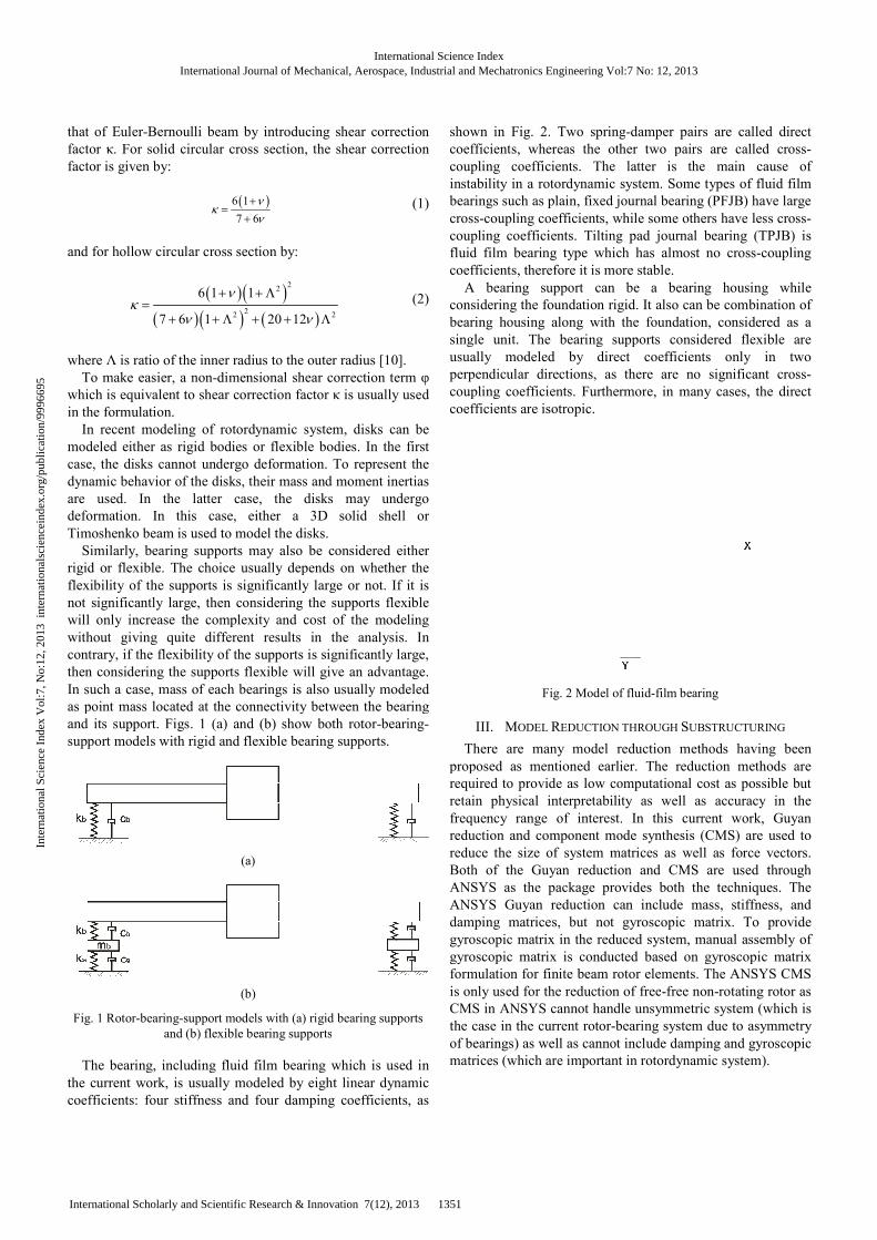
In such a case, mass of each bearings is also usually modeled
as point mass located at the connectivity between the bearing
and its support. Figs. 1 (a) and (b) show both rotor
support models with rigid and flexible bearing supports.
(a)
(b)
Fig. 1 Rotor-bearing-support models with (a) rigid bearing supports
and (b) flexible bearing supports
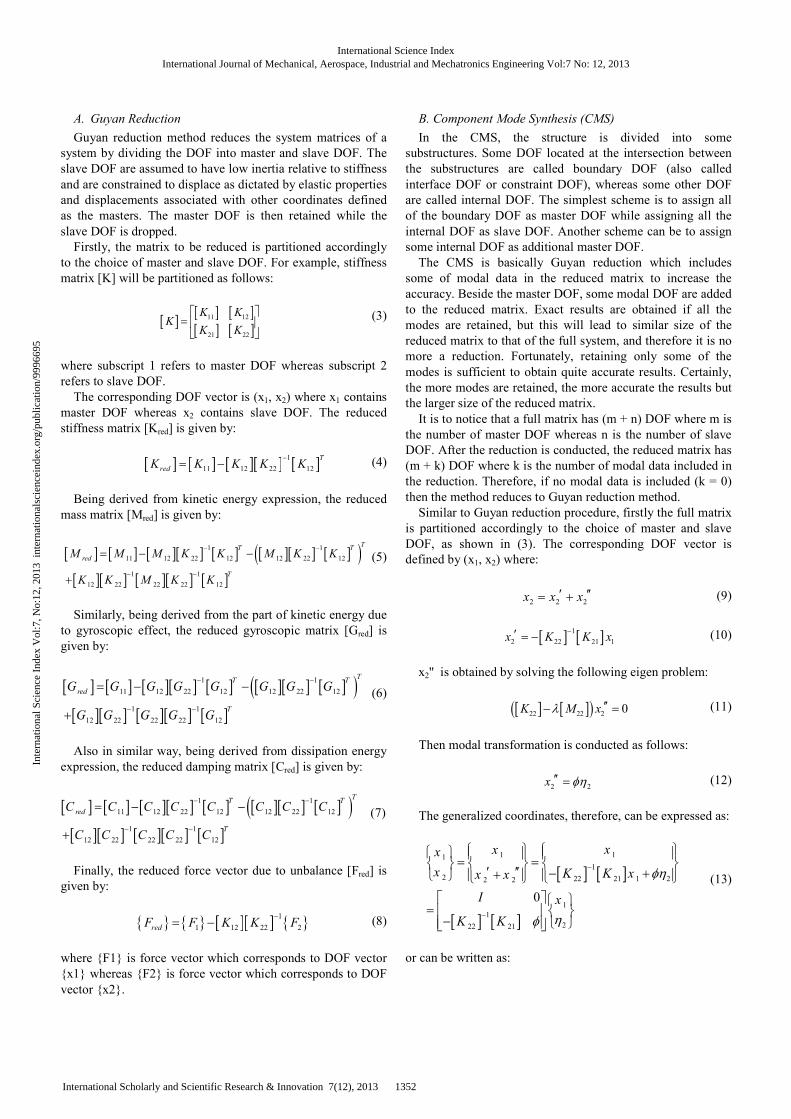
The bearing, including fluid film bearing which is used in
the current work, is usually modeled by eight linear dynamic
coefficients: four stiffness and four damping coefficients, as
ducing shear correction
factor κ. For solid circular cross section, the shear correction
(1)
)2 27 6 1 20 12ν ν+ + Λ + + Λ
(2)
where Λ is ratio of the inner radius to the outer radius [10].
dimensional shear correction term φ
which is equivalent to shear correction factor κ is usually used
ic system, disks can be
modeled either as rigid bodies or flexible bodies. In the first
case, the disks cannot undergo deformation. To represent the
dynamic behavior of the disks, their mass and moment inertias
are used. In the latter case, the disks may undergo
deformation. In this case, either a 3D solid shell or
eam is used to model the disks.
Similarly, bearing supports may also be considered either
rigid or flexible. The choice usually depends on whether the
ignificantly large or not. If it is
not significantly large, then considering the supports flexible
will only increase the complexity and cost of the modeling
without giving quite different results in the analysis. In
pports is significantly large,
then considering the supports flexible will give an advantage.
In such a case, mass of each bearings is also usually modeled
as point mass located at the connectivity between the bearing
how both rotor-bearing-
support models with rigid and flexible bearing supports.
support models with (a) rigid bearing supports
and (b) flexible bearing supports
The bearing, including fluid film bearing which is used in
the current work, is usually modeled by eight linear dynamic
coefficients: four stiffness and four damping coefficients, as
shown in Fig. 2. Two spring
coefficients, whereas the other two pairs are called cross
coupling coefficients. The latter is the main cause of
instability in a rotordynamic system. Some types of fluid film
bearings such as plain, fixed journal bearing (PFJB) have large
cross-coupling coefficients, while some others have less cross
coupling coefficients. Tilting pad journal bearing (TPJB) is
fluid film bearing type which has almost no cross
coefficients, therefore it is more stable.
A bearing support can be a bearing housing while
considering the foundation rigid. It also can be combination of
bearing housing along with the foundation, considered as a
single unit. The bearing supports considered flexible are
usually modeled by direct coefficients only in two
perpendicular directions, as there are no significant cross
coupling coefficients. Furthermor
coefficients are isotropic.
Fig. 2 Model of fluid
III. MODEL REDUCTION
There are many model reduction methods having been
proposed as mentioned earlier. The reduction methods are
required to provide as low computational cost as possible but
retain physical interpretability as well as accuracy in the
frequency range of interest. In this current work, Guyan
reduction and component mode synthesis (CMS) are used to
reduce the size of system matrices
Both of the Guyan reduction and CMS are used through
ANSYS as the package provides both the techniques. The
ANSYS Guyan reduction can include mass, stiffness, and
damping matrices, but not gyroscopic matrix. To provide
gyroscopic matrix in the reduced system, manual assembly of
gyroscopic matrix is conducted based on gyroscopic matrix
formulation for finite beam rotor elements. The ANSYS CMS
is only used for the reduction of free
CMS in ANSYS cannot hand
the case in the current rotor-bearing system due to asymmetry
of bearings) as well as cannot include damping and gyroscopic
matrices (which are important in rotordynamic system).
2. Two spring-damper pairs are called direct
coefficients, whereas the other two pairs are called cross-
icients. The latter is the main cause of
instability in a rotordynamic system. Some types of fluid film
bearings such as plain, fixed journal bearing (PFJB) have large
coupling coefficients, while some others have less cross-
lting pad journal bearing (TPJB) is
fluid film bearing type which has almost no cross-coupling
coefficients, therefore it is more stable.
A bearing support can be a bearing housing while
considering the foundation rigid. It also can be combination of
ng housing along with the foundation, considered as a
single unit. The bearing supports considered flexible are
usually modeled by direct coefficients only in two
perpendicular directions, as there are no significant cross-
coupling coefficients. Furthermore, in many cases, the direct
2 Model of fluid-film bearing
EDUCTION THROUGH SUBSTRUCTURING
There are many model reduction methods having been
proposed as mentioned earlier. The reduction methods are
ovide as low computational cost as possible but
retain physical interpretability as well as accuracy in the
frequency range of interest. In this current work, Guyan
reduction and component mode synthesis (CMS) are used to
reduce the size of system matrices as well as force vectors.
Both of the Guyan reduction and CMS are used through
ANSYS as the package provides both the techniques. The
ANSYS Guyan reduction can include mass, stiffness, and
damping matrices, but not gyroscopic matrix. To provide
matrix in the reduced system, manual assembly of
gyroscopic matrix is conducted based on gyroscopic matrix
formulation for finite beam rotor elements. The ANSYS CMS
is only used for the reduction of free-free non-rotating rotor as
CMS in ANSYS cannot handle unsymmetric system (which is
bearing system due to asymmetry
of bearings) as well as cannot include damping and gyroscopic
matrices (which are important in rotordynamic system).
International Science IndexInternational Journal of Mechanical, Aerospace, Industrial and Mechatronics Engineering Vol:7 No: 12, 2013
1351International Scholarly and Scientific Research & Innovation 7(12), 2013
Inte
rnat
iona
l Sci
ence
Ind
ex V
ol:7
, No:
12, 2
013
inte
rnat
iona
lsci
ence
inde
x.or
g/pu
blic
atio
n/99
9669
5
A. Guyan Reduction
Guyan reduction method reduces the system matrices of a
system by dividing the DOF into master and slave DOF. The
slave DOF are assumed to have low inertia relative to stiffness
and are constrained to displace as dictated by elastic properties
and displacements associated with other coordinates defined
as the masters. The master DOF is then retained while the
slave DOF is dropped.
Firstly, the matrix to be reduced is partitioned accordingly
to the choice of master and slave DOF. For example, stiffness
matrix [K] will be partitioned as follows:
[ ] [ ] [ ][ ] [ ]
11 12
21 22
K KK
K K
=
(3)
where subscript 1 refers to master DOF whereas subscript 2
refers to slave DOF.
The corresponding DOF vector is (x1, x2) where x1 contains
master DOF whereas x2 contains slave DOF. The reduced
stiffness matrix [Kred] is given by:
[ ] [ ] [ ][ ] [ ]1
11 12 22 12
T
redK K K K K−
= − (4)
Being derived from kinetic energy expression, the reduced
mass matrix [Mred] is given by:
[ ] [ ] [ ][ ] [ ] [ ][ ] [ ]( )[ ][ ] [ ][ ] [ ]
1 1
11 12 22 12 12 22 12
1 1
12 22 22 22 12
TT T
red
T
M M M K K M K K
K K M K K
− −
− −
= − −
+
(5)
Similarly, being derived from the part of kinetic energy due
to gyroscopic effect, the reduced gyroscopic matrix [Gred] is
given by:
[ ] [ ] [ ][ ] [ ] [ ][ ] [ ]( )[ ][ ] [ ][ ] [ ]
1 1
11 12 22 12 12 22 12
1 1
12 22 22 22 12
TT T
red
T
G G G G G G G G
G G G G G
− −
− −
= − −
+
(6)
Also in similar way, being derived from dissipation energy
expression, the reduced damping matrix [Cred] is given by:
[ ] [ ] [ ][ ] [ ] [ ][ ] [ ]( )[ ][ ] [ ][ ] [ ]
1 1
11 12 22 12 12 22 12
1 1
12 22 22 22 12
TT T
red
T
C C C C C C C C
C C C C C
− −
− −
= − −
+
(7)
Finally, the reduced force vector due to unbalance [Fred] is
given by:
{ } { } [ ][ ] { }1
1 12 22 2redF F K K F−
= − (8)
where {F1} is force vector which corresponds to DOF vector
{x1} whereas {F2} is force vector which corresponds to DOF
vector {x2}.
B. Component Mode Synthesis (CMS)
In the CMS, the structure is divided into some
substructures. Some DOF located at the intersection between
the substructures are called boundary DOF (also called
interface DOF or constraint DOF), whereas some other DOF
are called internal DOF. The simplest scheme is to assign all
of the boundary DOF as master DOF while assigning all the
internal DOF as slave DOF. Another scheme can be to assign
some internal DOF as additional master DOF.
The CMS is basically Guyan reduction which includes
some of modal data in the reduced matrix to increase the
accuracy. Beside the master DOF, some modal DOF are added
to the reduced matrix. Exact results are obtained if all the
modes are retained, but this will lead to similar size of the
reduced matrix to that of the full system, and therefore it is no
more a reduction. Fortunately, retaining only some of the
modes is sufficient to obtain quite accurate results. Certainly,
the more modes are retained, the more accurate the results but
the larger size of the reduced matrix.
It is to notice that a full matrix has (m + n) DOF where m is
the number of master DOF whereas n is the number of slave
DOF. After the reduction is conducted, the reduced matrix has
(m + k) DOF where k is the number of modal data included in
the reduction. Therefore, if no modal data is included (k = 0)
then the method reduces to Guyan reduction method.
Similar to Guyan reduction procedure, firstly the full matrix
is partitioned accordingly to the choice of master and slave
DOF, as shown in (3). The corresponding DOF vector is
defined by (x1, x2) where:
2 2 2x x x′ ′′= + (9)
[ ] [ ]1
2 22 21 1x K K x−′ = − (10)
x2'' is obtained by solving the following eigen problem:
[ ] [ ]( )22 22 20K M xλ ′′− = (11)
Then modal transformation is conducted as follows:
2 2x φη′′ = (12)
The generalized coordinates, therefore, can be expressed as:
[ ] [ ]
[ ] [ ]
111
1
2 22 21 1 22 2
1
1
222 21
0
xxx
x K K xx x
I x
K K
φη
ηφ
−
−
= = ′ ′′ − ++
=
−
(13)
or can be written as:
International Science IndexInternational Journal of Mechanical, Aerospace, Industrial and Mechatronics Engineering Vol:7 No: 12, 2013
1352International Scholarly and Scientific Research & Innovation 7(12), 2013
Inte
rnat
iona
l Sci
ence
Ind
ex V
ol:7
, No:
12, 2
013
inte
rnat
iona
lsci
ence
inde
x.or
g/pu
blic
atio
n/99
9669
5
[ ]1 1
2 2
x x
xψ
η
=
(14)
where is called transformation matrix and given by:
[ ][ ] [ ]1
22 21
0I
K Kψ
φ−
=
−
(15)
by using the transformation matrix Ψ, the reduced matrices are
defined by:
[ ] [ ] [ ][ ]T
redM Mψ ψ= (16)
[ ] [ ] [ ][ ]T
redK Kψ ψ= (17)
[ ] [ ] [ ][ ]T
redG Gψ ψ= (18)
[ ] [ ] [ ][ ]T
redC Cψ ψ= (19)
{ } [ ] { }T
redF Fψ= (20)
C. Substructuring in ANSYS
Guyan reduction and CMS can be conducted using
substructuring in ANSYS. Substructuring is a procedure that
condenses a group of finite elements into one element
represented as a matrix. The single-matrix element is called a
superelement. Substructuring reduces computer time and
allows solution of large problems with limited computer
resources. The substructure analysis uses the technique of
matrix reduction to reduce the system matrices to a smaller set
of DOF. In the substructuring, the superelements are created to
result in reduced number of DOF.
General substructuring in ANSYS uses Guyan reduction
procedure to calculate the reduced matrices. The key
assumption in this procedure is that for the lower frequencies,
inertia forces on the slave degrees of freedom (those degrees
of freedom being reduced out) are negligible compared to
elastic forces transmitted by the master degrees of freedom
(MDOF). Therefore, the total mass of the structure is
apportioned among only the MDOF. The net result is that the
reduced stiffness matrix is exact, whereas the reduced mass
and damping matrices are approximate. Guyan reduction in
ANSYS is improved so that it can include damping matrix.
A special substructuring using CMS is also available in
ANSYS. However, CMS in ANSYS now does not yet include
damping matrix although in theory the CMS can include the
damping matrix. Furthermore, CMS in ANSYS only work
with symmetric matrix. In general, CMS gives better reduction
for higher frequencies because it includes the modal data in
the reduction process. However, the reduced matrices can be
larger as some additional DOF coming from the modal data
are added in the matrices.
In superelements, some master nodes have to be selected.
Selecting the master nodes is an important step in a reduced
analysis. The accuracy of the reduced mass matrix (and hence
the accuracy of the solution) depends on the number and
location of masters. The master nodes are selected based on
the following guidelines:
1) The total number of MDOF should be at least twice the
number of modes of interest.
2) Selected MDOF should be in directions in which the
structure or component is expected to vibrate.
3) Zero lateral displacement are assigned as master nodes.
4) Nodes at which forces are applied are assigned as master
nodes.
5) Nodes at which inertia is relatively large and stiffness is
relatively low are assigned as master nodes.
Substructuring involves three distinct steps called passes:
(1) generation pass, (2) use pass, and (3) expansion pass. The
generation pass is condensing a group of "regular" finite
elements into a single superelement. The condensation is done
by identifying a set of MDOF. The procedure to generate a
superelement consists of two main steps: (1) building the
model and (2) applying loads and creating the superelement
matrices.
The use pass is using the superelement in an analysis by
making it part of the model. The entire model may be a
superelement, or, the superelement may be connected to other
nonsuperelements. The solution from the use pass consists
only of the reduced solution for the superelement and
complete solution for nonsuperelements.
The expansion pass is starting with the reduced solution and
calculating the results at all DOF in the superelement. If
multiple superelements are used in the use pass, a separate
expansion pass will be required for each superelement. The
backsubstitution method uses the reduced solution from the
use pass and substitutes it back into the available factorized
matrix file to calculate the complete solution.
Based on how the substructuring is conducted, there are two
kinds of substructuring which can be conducted in ANSYS.
The first is called bottom-up substructuring, meaning that each
superelement is separately generated in an individual
generation pass, and all superelements are assembled together
in the use pass. This method is suitable for very large models
which are divided into smaller superelements so that they can
"fit" on the computer.
The second is called top-down substructuring. This is
suitable for substructuring of smaller models. An advantage of
this method is that the results for multiple superelements can
be assembled in postprocessing. The procedure for top-down
substructuring is in general similar to that of bottom-up
substructuring. What makes the top-down substructuring
different is that the whole model is built first.
IV. NUMERICAL EXAMPLE
In the following example, a rotor-bearing-support system of
a steam turbine, which has been analyzed in a previous work
[11], is used. Some data and results of the previous work are
International Science IndexInternational Journal of Mechanical, Aerospace, Industrial and Mechatronics Engineering Vol:7 No: 12, 2013
1353International Scholarly and Scientific Research & Innovation 7(12), 2013
Inte
rnat
iona
l Sci
ence
Ind
ex V
ol:7
, No:
12, 2
013
inte
rnat
iona
lsci
ence
inde
x.or
g/pu
blic
atio
n/99
9669
5
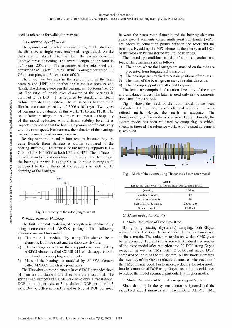
used as reference for validation purpose.
A. Component Specifications
The geometry of the rotor is shown in Fig. 3. The shaft and
the disks are a single piece machined, forged steel. As the
disks are not shrunk into the shaft, the system does not
undergo stress stiffening. The overall length of the rotor is
524.56cm (206.52in). The properties of the rotor steel are:
density of 8450 kg/m3 (0.30531 lb/in
3), Young modulus of 190
GPa (isotropic), and Poisson ratio of 0.3.
There are two bearings in the system: one at the high
pressure end (HPE) and another one at the low pressure end
(LPE). The distance between the bearings is 410.36cm (161.56
in). The ratio of length over diameter of the bearings is
assumed to be L/D = 1 as required by standard for steam
turbine rotor-bearing system. The oil used as bearing fluid
film has a constant viscosity = 2.3206 x 10⁻⁶
reyns. Two types
of bearings are evaluated in this work: TPJB and PFJB. The
two different bearings are used in order to evaluate the quality
of the model reduction with different stability level. It is
important to notice that the bearing dynamic coefficients vary
with the rotor speed. Furthermore, the behavior of the bearings
makes the overall system unsymmetric.
Bearing supports are taken into account because they are
quite flexible (their stiffness is worthy compared to the
bearing stiffness). The stiffness of the bearing supports is 1.4
GN/m (8.0 x 10⁶ lb/in) at both LPE and HPE. The stiffness in
horizontal and vertical direction are the same. The damping of
the bearing supports is negligible as its value is very small
compared to the stiffness of the supports as well as the
damping of the bearings.
Fig. 3 Geometry of the rotor (length in cm)
B. Finite Element Modeling
The finite element modeling of the system is conducted by
using non-commercial ANSYS package. The following
elements are used for modeling:
1) The rotor is modeled by using Timoshenko beam
elements. Both the shaft and the disks are flexible.
2) The bearings as well as their supports are modeled by
ANSYS element called COMBI214 which supports both
direct and cross-coupling coefficients.
3) Mass of the bearings is modeled by ANSYS element
called MASS21 which is a point mass.
The Timoshenko rotor elements have 6 DOF per node: three
of them are translational and three others are rotational. The
springs and dampers in COMBI214 have only 1 translational
DOF per node per axis, or 3 translational DOF per node in 3
axis. Due to different number and/or type of DOF per node
between the beam rotor elements and the bearing elements,
some special elements called multi-point constraints (MPC)
are added at connection points between the rotor and the
bearings. By adding the MPC elements, the energy in all DOF
of the rotor can be transferred well to the bearings.
The boundary conditions consist of some constraints and
loads. The constraints are as follows:
1) The nodes where the bearings are attached on the axis are
prevented from longitudinal translation.
2) The bearings are attached to certain positions of the axis.
3) The mass of the bearings can move in radial direction.
4) The bearing supports are attached to ground.
The loads are comprised of rotational velocity of the rotor
and unbalance forces. The latter is used only in the harmonic
unbalance force analysis.
Fig. 4 shows the mesh of the rotor model. It has been
evaluated that the mesh gives identical response to more
refined mesh. Hence, the mesh is adequate. The
dimensionality of the model is shown in Table I. Finally, the
system model has been validated by comparing its critical
speeds to those of the reference work. A quite good agreement
is achieved.
Fig. 4 Mesh of the system using Timoshenko beam rotor model
TABLE I
DIMENSIONALITY OF THE FINITE ELEMENT ROTOR MODEL
Quantity Value
Number of nodes 99
Number of elements 49
Size of M, C, K matrix 1230 x 1230
Size of F vector 1230 x 1
C. Model Reduction Results
1. Model Reduction of Free-Free Rotor
By ignoring rotating (hysteretic) damping, both Guyan
reduction and CMS can be used to create reduced mass and
stiffness matrix. The reduction results show that CMS gives
better accuracy. Table II shows some first natural frequencies
of the rotor model after reduction into 30 DOF using Guyan
reduction as well as CMS with 12 additional modal DOF,
compared to those of the full system. As the mode increases,
the accuracy of the Guyan reduction decreases whereas that of
the CMS remains good. Furthermore, reducing the rotor model
into less number of DOF using Guyan reduction is evidenced
to reduce the model accuracy, particularly at higher modes.
2. Model Reduction of Rotor-Bearing-Support System
Since damping in the system cannot be ignored and the
assembled global matrices are unsymmetric, ANSYS CMS
International Science IndexInternational Journal of Mechanical, Aerospace, Industrial and Mechatronics Engineering Vol:7 No: 12, 2013
1354International Scholarly and Scientific Research & Innovation 7(12), 2013
Inte
rnat
iona
l Sci
ence
Ind
ex V
ol:7
, No:
12, 2
013
inte
rnat
iona
lsci
ence
inde
x.or
g/pu
blic
atio
n/99
9669
5
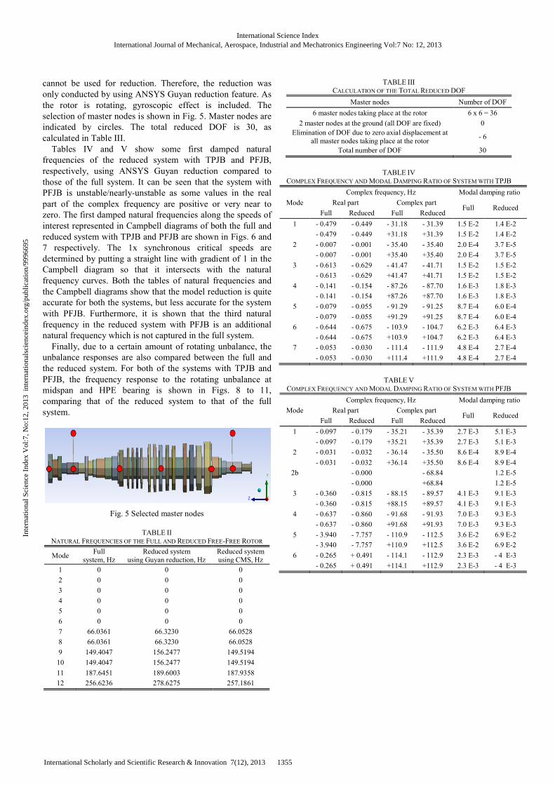
cannot be used for reduction. Therefore, the reduction was
only conducted by using ANSYS Guyan reduction feature. As
the rotor is rotating, gyroscopic effect is included. The
selection of master nodes is shown in Fig. 5. Master nodes are
indicated by circles. The total reduced DOF is 30, as
calculated in Table III.
Tables IV and V show some first damped natural
frequencies of the reduced system with TPJB and PFJB,
respectively, using ANSYS Guyan reduction compared to
those of the full system. It can be seen that the system with
PFJB is unstable/nearly-unstable as some values in the real
part of the complex frequency are positive or very near to
zero. The first damped natural frequencies along the speeds of
interest represented in Campbell diagrams of both the full and
reduced system with TPJB and PFJB are shown in Figs. 6 and
7 respectively. The 1x synchronous critical speeds are
determined by putting a straight line with gradient of 1 in the
Campbell diagram so that it intersects with the natural
frequency curves. Both the tables of natural frequencies and
the Campbell diagrams show that the model reduction is quite
accurate for both the systems, but less accurate for the system
with PFJB. Furthermore, it is shown that the third natural
frequency in the reduced system with PFJB is an additional
natural frequency which is not captured in the full system.
Finally, due to a certain amount of rotating unbalance, the
unbalance responses are also compared between the full and
the reduced system. For both of the systems with TPJB and
PFJB, the frequency response to the rotating unbalance at
midspan and HPE bearing is shown in Figs. 8 to 11,
comparing that of the reduced system to that of the full
system.
Fig. 5 Selected master nodes
TABLE II
NATURAL FREQUENCIES OF THE FULL AND REDUCED FREE-FREE ROTOR
Mode Full
system, Hz
Reduced system
using Guyan reduction, Hz
Reduced system
using CMS, Hz
1 0 0 0
2 0 0 0
3 0 0 0
4 0 0 0
5 0 0 0
6 0 0 0
7 66.0361 66.3230 66.0528
8 66.0361 66.3230 66.0528
9 149.4047 156.2477 149.5194
10 149.4047 156.2477 149.5194
11 187.6451 189.6003 187.9358
12 256.6236 278.6275 257.1861
TABLE III
CALCULATION OF THE TOTAL REDUCED DOF
Master nodes Number of DOF
6 master nodes taking place at the rotor 6 x 6 = 36
2 master nodes at the ground (all DOF are fixed) 0
Elimination of DOF due to zero axial displacement at
all master nodes taking place at the rotor - 6
Total number of DOF 30
TABLE IV
COMPLEX FREQUENCY AND MODAL DAMPING RATIO OF SYSTEM WITH TPJB
Mode
Complex frequency, Hz Modal damping ratio
Real part Complex part Full Reduced
Full Reduced Full Reduced
1 - 0.479 - 0.449 - 31.18 - 31.39 1.5 E-2 1.4 E-2
- 0.479 - 0.449 +31.18 +31.39 1.5 E-2 1.4 E-2
2 - 0.007 - 0.001 - 35.40 - 35.40 2.0 E-4 3.7 E-5
- 0.007 - 0.001 +35.40 +35.40 2.0 E-4 3.7 E-5
3 - 0.613 - 0.629 - 41.47 - 41.71 1.5 E-2 1.5 E-2
- 0.613 - 0.629 +41.47 +41.71 1.5 E-2 1.5 E-2
4 - 0.141 - 0.154 - 87.26 - 87.70 1.6 E-3 1.8 E-3
- 0.141 - 0.154 +87.26 +87.70 1.6 E-3 1.8 E-3
5 - 0.079 - 0.055 - 91.29 - 91.25 8.7 E-4 6.0 E-4
- 0.079 - 0.055 +91.29 +91.25 8.7 E-4 6.0 E-4
6 - 0.644 - 0.675 - 103.9 - 104.7 6.2 E-3 6.4 E-3
- 0.644 - 0.675 +103.9 +104.7 6.2 E-3 6.4 E-3
7 - 0.053 - 0.030 - 111.4 - 111.9 4.8 E-4 2.7 E-4
- 0.053 - 0.030 +111.4 +111.9 4.8 E-4 2.7 E-4
TABLE V
COMPLEX FREQUENCY AND MODAL DAMPING RATIO OF SYSTEM WITH PFJB
Mode
Complex frequency, Hz Modal damping ratio
Real part Complex part Full Reduced
Full Reduced Full Reduced
1 - 0.097 - 0.179 - 35.21 - 35.39 2.7 E-3 5.1 E-3
- 0.097 - 0.179 +35.21 +35.39 2.7 E-3 5.1 E-3
2 - 0.031 - 0.032 - 36.14 - 35.50 8.6 E-4 8.9 E-4
- 0.031 - 0.032 +36.14 +35.50 8.6 E-4 8.9 E-4
2b - 0.000 - 68.84 1.2 E-5
- 0.000 +68.84 1.2 E-5
3 - 0.360 - 0.815 - 88.15 - 89.57 4.1 E-3 9.1 E-3
- 0.360 - 0.815 +88.15 +89.57 4.1 E-3 9.1 E-3
4 - 0.637 - 0.860 - 91.68 - 91.93 7.0 E-3 9.3 E-3
- 0.637 - 0.860 +91.68 +91.93 7.0 E-3 9.3 E-3
5 - 3.940 - 7.757 - 110.9 - 112.5 3.6 E-2 6.9 E-2
- 3.940 - 7.757 +110.9 +112.5 3.6 E-2 6.9 E-2
6 - 0.265 + 0.491 - 114.1 - 112.9 2.3 E-3 - 4 E-3
- 0.265 + 0.491 +114.1 +112.9 2.3 E-3 - 4 E-3
International Science IndexInternational Journal of Mechanical, Aerospace, Industrial and Mechatronics Engineering Vol:7 No: 12, 2013
1355International Scholarly and Scientific Research & Innovation 7(12), 2013
Inte
rnat
iona
l Sci
ence
Ind
ex V
ol:7
, No:
12, 2
013
inte
rnat
iona
lsci
ence
inde
x.or
g/pu
blic
atio
n/99
9669
5
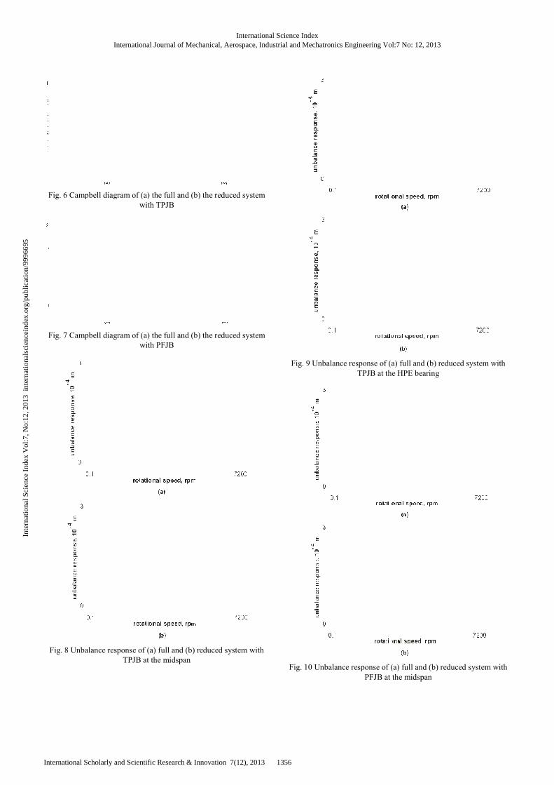
Fig. 6 Campbell diagram of (a) the full and (b) the reduced system
with TPJB
Fig. 7 Campbell diagram of (a) the full and (b) the reduced system
with PFJB
Fig. 8 Unbalance response of (a) full and (b) reduced system with
TPJB at the midspan
6 Campbell diagram of (a) the full and (b) the reduced system
(b) the reduced system
Unbalance response of (a) full and (b) reduced system with
Fig. 9 Unbalance response of (a) full and (b) reduced system with
TPJB at the HPE bearin
Fig. 10 Unbalance response of (a) full and (b) reduced system with
PFJB at the midspan
Unbalance response of (a) full and (b) reduced system with
TPJB at the HPE bearing
Unbalance response of (a) full and (b) reduced system with
PFJB at the midspan
International Science IndexInternational Journal of Mechanical, Aerospace, Industrial and Mechatronics Engineering Vol:7 No: 12, 2013
1356International Scholarly and Scientific Research & Innovation 7(12), 2013
Inte
rnat
iona
l Sci
ence
Ind
ex V
ol:7
, No:
12, 2
013
inte
rnat
iona
lsci
ence
inde
x.or
g/pu
blic
atio
n/99
9669
5
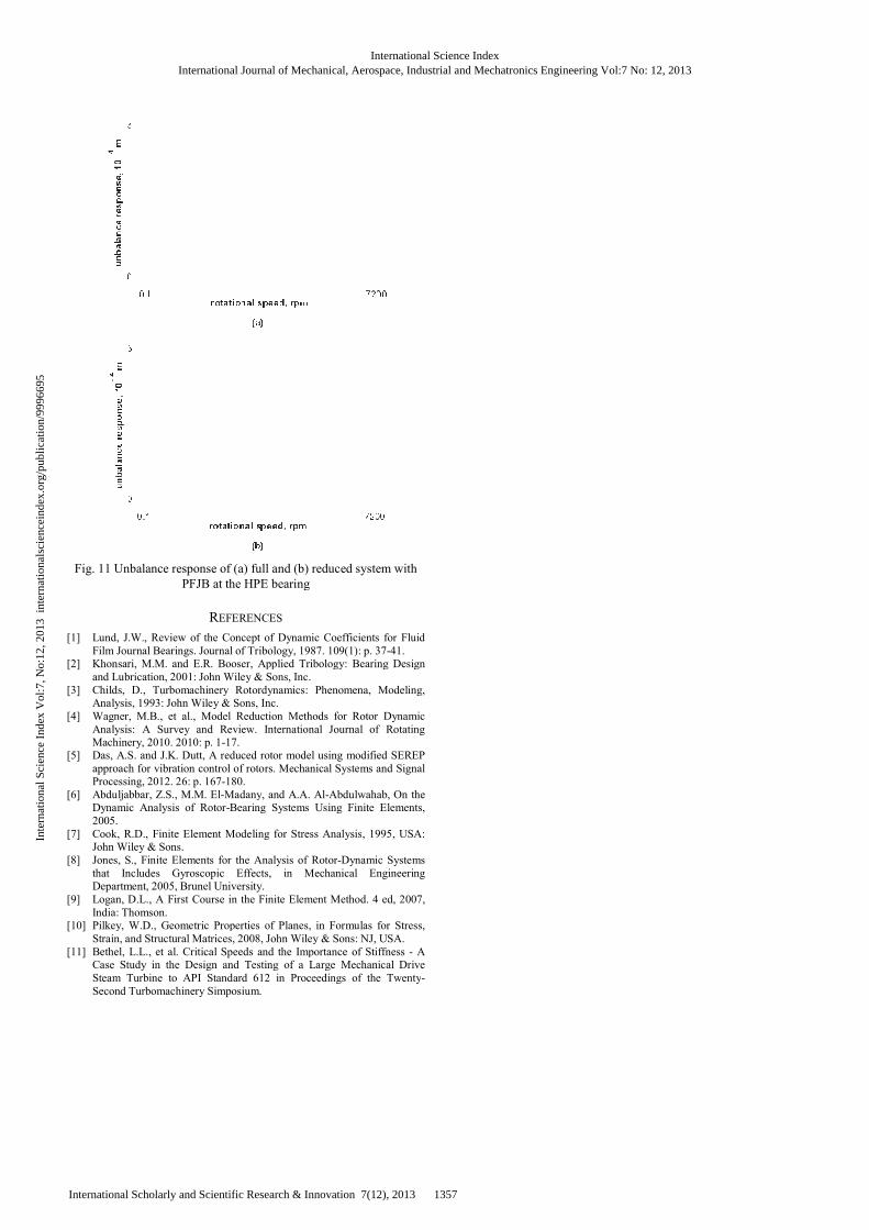
Fig. 11 Unbalance response of (a) full and (b) reduced system with
PFJB at the HPE bearing
REFERENCES
[1] Lund, J.W., Review of the Concept of Dynamic Coefficients fo
Film Journal Bearings. Journal of Tribology, 1987. 109(1): p. 37[2] Khonsari, M.M. and E.R. Booser, Applied Tribology: Bearing Design
and Lubrication, 2001: John Wiley & Sons, Inc.
[3] Childs, D., Turbomachinery Rotordynamics: Phenomena, Modeling, Analysis, 1993: John Wiley & Sons, Inc.
[4] Wagner, M.B., et al., Model Reduction Methods for Rotor Dynamic
Analysis: A Survey and Review. International Journal of Rotating Machinery, 2010. 2010: p. 1-17.
[5] Das, A.S. and J.K. Dutt, A reduced rotor model using modif
approach for vibration control of rotors. Mechanical Systems and Signal Processing, 2012. 26: p. 167-180.
[6] Abduljabbar, Z.S., M.M. El-Madany, and A.A. AlDynamic Analysis of Rotor-Bearing Systems Using Finite Elements,
2005.
[7] Cook, R.D., Finite Element Modeling for Stress AnalysisJohn Wiley & Sons.
[8] Jones, S., Finite Elements for the Analysis of Rotor
that Includes Gyroscopic Effects, in Mechanical Engineering Department, 2005, Brunel University.
[9] Logan, D.L., A First Course in the Finite Element Method. 4 ed
India: Thomson. [10] Pilkey, W.D., Geometric Properties of Planes, in Formulas for Stress,
Strain, and Structural Matrices, 2008, John Wiley & Sons: NJ, USA.
[11] Bethel, L.L., et al. Critical Speeds and the Importance of Stiffness Case Study in the Design and Testing of a Large Mechanical Drive
Steam Turbine to API Standard 612 in Proceedings of the Twenty
Second Turbomachinery Simposium.
Unbalance response of (a) full and (b) reduced system with
PFJB at the HPE bearing
Lund, J.W., Review of the Concept of Dynamic Coefficients for Fluid
Film Journal Bearings. Journal of Tribology, 1987. 109(1): p. 37-41. Khonsari, M.M. and E.R. Booser, Applied Tribology: Bearing Design
2001: John Wiley & Sons, Inc.
Childs, D., Turbomachinery Rotordynamics: Phenomena, Modeling,
Wagner, M.B., et al., Model Reduction Methods for Rotor Dynamic
Analysis: A Survey and Review. International Journal of Rotating
Das, A.S. and J.K. Dutt, A reduced rotor model using modified SEREP
approach for vibration control of rotors. Mechanical Systems and Signal
Madany, and A.A. Al-Abdulwahab, On the g Systems Using Finite Elements,
k, R.D., Finite Element Modeling for Stress Analysis, 1995, USA:
Jones, S., Finite Elements for the Analysis of Rotor-Dynamic Systems
that Includes Gyroscopic Effects, in Mechanical Engineering
Logan, D.L., A First Course in the Finite Element Method. 4 ed, 2007,
Pilkey, W.D., Geometric Properties of Planes, in Formulas for Stress,
2008, John Wiley & Sons: NJ, USA.
eds and the Importance of Stiffness - A Case Study in the Design and Testing of a Large Mechanical Drive
in Proceedings of the Twenty-
International Science IndexInternational Journal of Mechanical, Aerospace, Industrial and Mechatronics Engineering Vol:7 No: 12, 2013
1357International Scholarly and Scientific Research & Innovation 7(12), 2013
Inte
rnat
iona
l Sci
ence
Ind
ex V
ol:7
, No:
12, 2
013
inte
rnat
iona
lsci
ence
inde
x.or
g/pu
blic
atio
n/99
9669
5
Related Documents


