REDUCTION, LINEARIZATION, AND STABILITY OF RELATIVE EQUILIBRIA FOR MECHANICAL SYSTEMS ON RIEMANNIAN MANIFOLDS FRANCESCO BULLO AND ANDREW D. LEWIS Abstract. Consider a Riemannian manifold equipped with an in- finitesimal isometry. For this setup, a unified treatment is provided, solely in the language of Riemannian geometry, of techniques in reduc- tion, linearization, and stability of relative equilibria. In particular, for mechanical control systems, an explicit characterization is given for the manner in which reduction by an infinitesimal isometry, and linearization along a controlled trajectory “commute.” As part of the development, relationships are derived between the Jacobi equation of geodesic variation and concepts from reduction theory, such as the curvature of the mechanical connection and the effective potential. As an application of our techniques, fiber and base stability of relative equilibria are studied. The paper also serves as a tutorial of Riemann- ian geometric methods applicable in the intersection of mechanics and control theory. 1. Introduction Mechanical systems with symmetry have been a focus of an enormous research effort during the past few decades. This reflects of the importance of the notion of symmetry in physics. Of particular importance are those trajectories of a dynamical system that are also orbits for the symmetry group of the problem; these are relative equilibria. The stability of relative equilibria has both theoretical and practical importance. From a theoretical point of view, the relative equilibria, and their associated stability analysis, often give important insight into global behavior of solutions. In practical applications, relative equilibria arise in such diverse areas as fluid mechan- ics and underwater vehicle dynamics. In such problems, one often desires stability of a given relative equilibrium. Should such a relative equilibrium be naturally unstable, one must then develop ways of stabilizing it using control theory. Date : 28/02/2005. 1

Welcome message from author
This document is posted to help you gain knowledge. Please leave a comment to let me know what you think about it! Share it to your friends and learn new things together.
Transcript

REDUCTION, LINEARIZATION, AND STABILITY OFRELATIVE EQUILIBRIA FOR MECHANICAL SYSTEMS
ON RIEMANNIAN MANIFOLDS
FRANCESCO BULLO AND ANDREW D. LEWIS
Abstract. Consider a Riemannian manifold equipped with an in-finitesimal isometry. For this setup, a unified treatment is provided,solely in the language of Riemannian geometry, of techniques in reduc-tion, linearization, and stability of relative equilibria. In particular,for mechanical control systems, an explicit characterization is givenfor the manner in which reduction by an infinitesimal isometry, andlinearization along a controlled trajectory “commute.” As part of thedevelopment, relationships are derived between the Jacobi equationof geodesic variation and concepts from reduction theory, such as thecurvature of the mechanical connection and the effective potential. Asan application of our techniques, fiber and base stability of relativeequilibria are studied. The paper also serves as a tutorial of Riemann-ian geometric methods applicable in the intersection of mechanics andcontrol theory.
1. Introduction
Mechanical systems with symmetry have been a focus of an enormousresearch effort during the past few decades. This reflects of the importanceof the notion of symmetry in physics. Of particular importance are thosetrajectories of a dynamical system that are also orbits for the symmetrygroup of the problem; these are relative equilibria. The stability of relativeequilibria has both theoretical and practical importance. From a theoreticalpoint of view, the relative equilibria, and their associated stability analysis,often give important insight into global behavior of solutions. In practicalapplications, relative equilibria arise in such diverse areas as fluid mechan-ics and underwater vehicle dynamics. In such problems, one often desiresstability of a given relative equilibrium. Should such a relative equilibriumbe naturally unstable, one must then develop ways of stabilizing it usingcontrol theory.
Date: 28/02/2005.
1

2 FRANCESCO BULLO AND ANDREW D. LEWIS
This paper is concerned with the analysis of relative equilibria for simplemechanical systems, i.e., those that are Lagrangian with kinetic energy mi-nus potential energy Lagrangians. More specifically, in the paper we exploresome of the Riemannian geometry associated with a system with symme-try in general, and a relative equilibrium in particular. Of course, muchwork has been done in this area, so let us locate our work in this bodyof literature. When talking about reduction using symmetry (as opposedto the more specific discussion of relative equilibria), one can work in aHamiltonian or Lagrangian setting. The Hamiltonian setting is perhaps themore developed, going back to work of Arnol’d [1966], and the symplecticreduction work of Marsden and Weinstein [1974] and Meyer [1973]. Thiswork has been presented in a fully developed manner in the books [Abrahamand Marsden 1978, Guillemin and Sternberg 1984, Marsden 1992, Marsdenand Ratiu 1999], for example. More recent research on Hamiltonian re-duction theory is concerned with so-called singular reduction theory, wherethe regularity assumptions of the earlier work are relaxed. We refer thereader to [Ortega and Ratiu 2004] for the literature in this area. The La-grangian theory of reduction is more recent, and we refer to the presentationin the book [Marsden and Ratiu 1999], and to the papers [Cendra, Marsden,Pekarsky, and Ratiu 2003, Cendra, Marsden, and Ratiu 2001] as represen-tative of the work in this area.
In the Hamiltonian theory of reduction using symmetry, the symplec-tic, or more generally Poisson, structure plays the prominent role. Indeed,much of the work in this area is concerned with general symplectic mani-folds rather than cotangent bundles. On the Lagrangian side, the emphasishas been on the reduction of variational principles, the motivation for thisbeing that variational principles are fundamental for Lagrangian mechanics.In this paper we focus on Lagrangians that are of the kinetic energy minuspotential energy form. For such Lagrangians, an important role is playedby the kinetic energy Riemannian metric and its attendant Levi-Civita con-nection. With this as motivation, we study reduction and relative equilibriastrictly in terms of Riemannian geometry. We do not wish to assert thatthe Riemannian geometry approach we give here is superior to the varia-tional approach; we too believe in the primacy of the variational principlein Lagrangian mechanics. However, the extra structure offered by the Rie-mannian metric does lead one to naturally ask whether a theory of reductionbased purely on Riemannian geometry is possible and, if so, revealing. Weshow that it is possible, and we believe that it is revealing. This is presentedin Section 3.
Another emphasis of this paper is linearization. We start this in a rathergeneral way. Since the stabilization of relative equilibria is of interest [Bullo
MECHANICAL SYSTEMS ON RIEMANNIAN MANIFOLDS 3
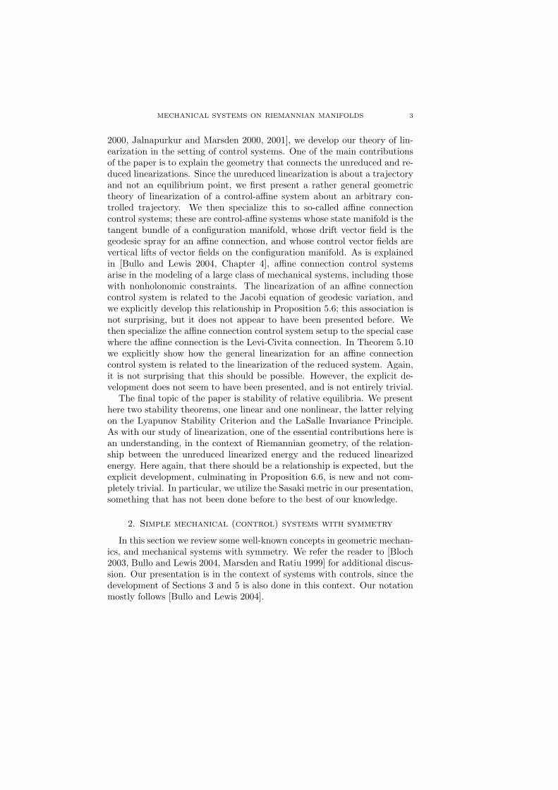
2000, Jalnapurkur and Marsden 2000, 2001], we develop our theory of lin-earization in the setting of control systems. One of the main contributionsof the paper is to explain the geometry that connects the unreduced and re-duced linearizations. Since the unreduced linearization is about a trajectoryand not an equilibrium point, we first present a rather general geometrictheory of linearization of a control-affine system about an arbitrary con-trolled trajectory. We then specialize this to so-called affine connectioncontrol systems; these are control-affine systems whose state manifold is thetangent bundle of a configuration manifold, whose drift vector field is thegeodesic spray for an affine connection, and whose control vector fields arevertical lifts of vector fields on the configuration manifold. As is explainedin [Bullo and Lewis 2004, Chapter 4], affine connection control systemsarise in the modeling of a large class of mechanical systems, including thosewith nonholonomic constraints. The linearization of an affine connectioncontrol system is related to the Jacobi equation of geodesic variation, andwe explicitly develop this relationship in Proposition 5.6; this association isnot surprising, but it does not appear to have been presented before. Wethen specialize the affine connection control system setup to the special casewhere the affine connection is the Levi-Civita connection. In Theorem 5.10we explicitly show how the general linearization for an affine connectioncontrol system is related to the linearization of the reduced system. Again,it is not surprising that this should be possible. However, the explicit de-velopment does not seem to have been presented, and is not entirely trivial.
The final topic of the paper is stability of relative equilibria. We presenthere two stability theorems, one linear and one nonlinear, the latter relyingon the Lyapunov Stability Criterion and the LaSalle Invariance Principle.As with our study of linearization, one of the essential contributions here isan understanding, in the context of Riemannian geometry, of the relation-ship between the unreduced linearized energy and the reduced linearizedenergy. Here again, that there should be a relationship is expected, but theexplicit development, culminating in Proposition 6.6, is new and not com-pletely trivial. In particular, we utilize the Sasaki metric in our presentation,something that has not been done before to the best of our knowledge.
2. Simple mechanical (control) systems with symmetry
In this section we review some well-known concepts in geometric mechan-ics, and mechanical systems with symmetry. We refer the reader to [Bloch2003, Bullo and Lewis 2004, Marsden and Ratiu 1999] for additional discus-sion. Our presentation is in the context of systems with controls, since thedevelopment of Sections 3 and 5 is also done in this context. Our notationmostly follows [Bullo and Lewis 2004].

4 FRANCESCO BULLO AND ANDREW D. LEWIS
Notation. In this section we quickly present some of the concepts andnotation we use.
If U and V are R-vector spaces, L(U; V) denotes the set of linear mapsfrom U to V.
Throughout the paper we work with manifolds and geometric objectthat are of class C∞, unless stated to the contrary. If M is a manifold,then C∞(M) denotes the set of C∞-functions on M. The tangent bun-dle of M is denoted by πTM : TM → M. If (x1, . . . , xn) are coordinatesfor M, then natural tangent bundle coordinates for TM are denoted by((x1, . . . , xn), (v1, . . . , vn)), or sometimes more compactly by (x,v). Thederivative of a map φ : M → N is denoted by Tφ : TM → TN, and the re-striction of the derivative to the tangent space TxM is denoted by Txφ. Ifπ : E → B is a vector bundle, then Γ∞(E) denotes the set of C∞-sections ofE. A vector field X : E → TE on the total space of a vector bundle π : E → Bis a linear vector field over a vector field X0 on B if X is π-related to X0
and if the following diagram commutes:
EX //
π
²²
TE
Tπ
²²B
X0
// TB
The zero section of a vector bundle E is denoted by Z(E). If B is a (0, 2)-tensor field on a manifold M, then B[ : TM → T∗M is the vector bundlemap defined by 〈B(ux); vx〉 = B(vx, ux) for ux, vx ∈ TM. If B[ in anisomorphism, then its inverse is denoted by B]. If G is a Riemannianmetric on M and if f ∈ C∞(M), then gradf denotes the vector field gradf =G] ◦df . Here df is the differential of f . Also, ‖·‖G denotes the norm onthe fibers of TM defined by G.
Typically, I ⊂ R will denote an interval. If γ : I → M is a differentiablecurve on M, then its tangent vector field is denoted by γ′ : I → TM. Acurve γ : I → M is locally absolutely continuous (abbreviated LAC ) iff ◦γ is locally absolutely continuous for every f ∈ C∞(M). If γ′ is LAC,then γ is locally absolutely differentiable (abbreviated LAD).
For a vector field X, the flow of X is denoted by (t, x) 7→ ΦX0,t(x), so
that the integral curve through x is t 7→ ΦX0,t(x). We will be considering
time-varying vector fields at various points in the paper, and since we wishto allow fairly general time-dependence, we should be precise about how wedo this. To this end, by a time-dependent vector field on M we shallmean a map X : I ×M → TM with the following properties:
(1) for each t ∈ I, the map Xt : x 7→ X(t, x) defines a C∞-vector field;

MECHANICAL SYSTEMS ON RIEMANNIAN MANIFOLDS 5
(2) for each x ∈ M, the map t 7→ X(t, x) is measurable (meaning itscomponents are measurable in some, and so any, set of coordinates);
(3) for each k ∈ \, each collection X1, . . . , Xk of C∞-vector fields on M,each C∞-one-form α on M, and each compact subset K ⊂ M, thereexists a positive locally integrable function ψ : I → R such that
|L X1 · · ·L Xk〈α; Xt〉 (x)| ≤ ψ(t), x ∈ K.
The usual Caratheodory theory shows that time-dependent vector fields de-fined in this fashion have LAC integral curves, and that their flows areof class C∞ with respect to initial conditions. We shall use the nota-tion (t, x) 7→ ΦX
0,t(x) to denote the flow of a time-dependent vector fieldX, i.e., we use the same notation for the flow of both time-independent andtime-dependent vector fields.
2.1. Simple mechanical (control) systems. A forced simple me-chanical control system is a 5-tuple Σ = (Q,G, V, F, F = {F 1, . . . , Fm})where
(1) Q is the configuration manifold , here assumed to be of puredimension n,
(2) G is the kinetic energy metric, which is a Riemannian metric onQ,
(3) V is the potential energy , a function on Q,(4) F : TQ → T∗Q is a bundle map over idQ, which is the external
force , and(5) {F 1, . . . , Fm} are the control forces, which are one-forms on Q.
The presentation in [Bullo and Lewis 2004] also includes an extra piece ofdata in the form of a set U ⊂ Rm where the control takes values. However,for the purposes of this paper, this is not important, so we do not includeit (that is to say, we take U = Rm). The equations governing a simplemechanical control system are
G∇γ′(t)γ
′(t) = −gradV (γ(t)) +G] ◦F (γ′(t)) +m∑
a=1
ua(t)G] ◦F a(γ(t)), (1)
whereG∇ is the Levi-Civita connection associated with G. We also denote
byGΓi
jk the Christoffel symbols forG∇. A controlled trajectory for Σ is
thus a pair (γ, u) where u : I → Rm is locally integrable and defined on aninterval I ⊂ R, and where γ : I → Q is LAD and satisfies (1).
Simple mechanical control systems are examples of a more general classof systems which we now introduce. A forced affine connection controlsystem is a 4-tuple (Q,∇, Y, Y = {Y1, . . . , Ym}), where
(1) Q is a manifold as above,

6 FRANCESCO BULLO AND ANDREW D. LEWIS
(2) ∇ is an affine connection on Q,(3) Y : TQ → TQ is a bundle map over idQ, and(4) {Y1, . . . , Ym} are vector fields on Q.
The equations governing such a system are
∇γ′(t)γ′(t) = Y (γ′(t)) +
m∑a=1
ua(t)Ya(γ(t)).
We can define the notion of a controlled trajectory for an affine connectionsystem in the same way as we did for a forced simple mechanical controlsystem. Moreover, note that a forced simple mechanical control system
is also a forced affine connection control system by taking ∇ =G∇, Y =
gradV ◦πTQ +G] ◦F . In [Bullo and Lewis 2004, Chapter 4] it is shown thataffine connection control systems model a large class of mechanical systems,including those with nonholonomic constraints.
Parts of the paper will be concerned with systems without forces, so letus introduce notation for these. A forced simple mechanical systemis a quadruple (Q,G, V, F ), where all the data are as for a forced simplemechanical control system. Of course, the governing equations are
G∇γ′(t)γ
′(t) = −gradV (γ(t)) +G] ◦F (γ′(t)).
If the external force F is omitted from list of data, the resulting triple(Q,G, V ) is a simple mechanical system .
2.2. Systems with symmetry. Now let us add symmetry to the aboveformulations. In this paper we shall only consider a single infinitesimal sym-metry, rather than the more usual situation where one considers symmetryof the system under a Lie group G. The extension of the results in the paperto this more general setup of a Lie group symmetry is currently ongoing.
Thus we consider a forced simple mechanical system Σ =(Q,G, V, F, F = {F 1, . . . , Fm}) and a vector field X on Q having the fol-lowing properties:
(1) X is an infinitesimal isometry for G, i.e., L XG = 0;(2) L XV = 0;(3) L X(F (Y )) = F (L XY ) for all vector fields Y on Q;(4) L XF a = 0 for a ∈ {1, . . . , m}.
A vector field X having these properties is an infinitesimal symmetryfor Σ. The infinitesimal symmetry X is complete if X is a complete vectorfield. A vector field having only property 1 is an infinitesimal isometryfor G.
Let us give some useful properties of infinitesimal isometries of G.

MECHANICAL SYSTEMS ON RIEMANNIAN MANIFOLDS 7
Proposition 2.1 (Characterization of infinitesimal isometry). Let (Q,G)be a Riemannian manifold. The following statements hold:
(i) the vector field X is an infinitesimal isometry if and only if the
covariant differentialG∇X is skew-symmetric with respect to G;
that is, for all Y,Z ∈ Γ∞(TQ),
G(Y,G∇ZX) +G(Z,
G∇Y X) = 0; (2)
(ii) if the vector field X is an infinitesimal isometry, then the functionq 7→ ‖X‖2G (q) is X-invariant and satisfies
12grad ‖X‖2G = −
G∇XX. (3)
Proof. Regarding part (i), we compute, for Y,Z ∈ Γ∞(TQ),
G(Y,G∇ZX) +G(Z,
G∇Y X) = G(Y,
G∇XZ + [Z,X]) +G(Z,
G∇XY + [Y,X])
= L X(G(Y,Z))−G(Y, [X, Z])−G(Z, [X, Y ])= (L XG)(Y, Z).
The result follows since this equality holds for all Y, Z ∈ Γ∞(TQ).To prove equation (3), let Z ∈ Γ∞(TQ) and compute
G(Z, grad ‖X‖2G) = L Z ‖X‖2G = 2G(X,G∇ZX) = −2G(Z,
G∇XX).
To show that q 7→ ‖X‖2G (q) is X-invariant, note that
L X ‖X‖2G = −2G(X,G∇XX) = 0.
¤
Associated to an infinitesimal isometry X for G is the X-momentummap JX : TQ → R defined by JX(vq) = G(X(q), vq). One can show [Bulloand Lewis 2004, Theorem 5.69] that the X-momentum map satisfies theevolution equation
ddt
JX(γ′(t)) =⟨Fu(t, γ′(t)); X(γ(t))
⟩
along a controlled trajectory (γ, u), where
Fu(t, vq) = F (vq) +∑a=1
ua(t)F a(vq).
In particular, if F = 0 and ua(t) = 0, a ∈ {1, . . . , m}, for all t, then theX-momentum is conserved; this is the Noether Conservation Law in thisparticular setup.

8 FRANCESCO BULLO AND ANDREW D. LEWIS
2.3. Relative equilibria. For mechanical systems with symmetry, relativeequilibria are important since they often give initial insights into the behav-ior of a system. In control theory, relative equilibria are often elementarymechanical motions that can be used as a basis for, for example, motionplanning. For additional discussion we refer to [Bloch 2003, Marsden 1992,Marsden and Ratiu 1999].
Definition 2.2 (Relative equilibrium). Let X be a complete infinitesimalsymmetry for Σ = (Q,G, V, F, F ) and let χ : R → Q be a maximal integralcurve of X.
(i) The curve χ is a relative equilibrium for Σ if it is a solution tothe equation of motion (27).
(ii) The relative equilibrium χ is regular if χ is an embedding. •To characterize relative equilibria, it is convenient to have the following
notion. We define the energy for a forced simple mechanical control systemΣ = (Q,G, V, F, F ) by E(vq) = 1
2G(vq, vq) + V (q).
Definition 2.3 (Effective energy). Let X be a complete infinitesimal sym-metry for Σ = (Q,G, V, F, F ), and let JX : TQ → R be the associatedmomentum map.
(i) The effective potential VX : Q → R is the function VX(q) =V (q)− 1
2 ‖X‖2G (q).(ii) The effective energy EX : TQ → R is the function EX(vq) =
E(vq)− JX(vq). •The following result characterizes the effective energy.
Lemma 2.4. EX(vq) = VX(q) + 12 ‖vq −X(q)‖2G.
Proof. The lemma is a consequence of the following “completing the square”computation:
E(vq)− JX(vq) = V (q) + 12 ‖vq‖2G −G(vq, X(q))
= V (q)− 12 ‖X‖2G (q)+ 1
2 ‖X‖2G (q)+ 12 ‖vq‖2G −G(vq, X(q))
= VX(q)+ 12 ‖vq−X(q)‖2G ,
as desired. ¤
Using this result, we can characterize relative equilibria as follows.
Proposition 2.5 (Existence of relative equilibria). Consider a forced simplemechanical system Σ = (Q,G, V, F ) and let X be a complete infinitesimalsymmetry for Σ. Then a maximal integral curve χ : R→ Q of X is a relativeequilibrium for Σ if and only if dVX(χ(t)) = F (χ′(t)) for some (and hence

MECHANICAL SYSTEMS ON RIEMANNIAN MANIFOLDS 9
for all) t ∈ R. In particular, if F (χ′(t)) = 0 for some (and hence for all)t ∈ R, then χ is a relative equilibrium for Σ if and only if VX has a criticalpoint at χ(t) for some (hence for all) t ∈ R.
Proof. We proceed in a direct way. Assume that χ is a maximal integralcurve of X. The curve χ satisfies the equations of motion (27) if and only if
0 =G∇χ′(t)χ
′(t) + gradV (χ(t))−G] ◦F (χ′(t))
=G∇X(χ(t))X(χ(t)) + gradV (χ(t))−G] ◦F (χ′(t))
= grad(− 1
2 ‖X‖2G + V)(χ(t))−G] ◦F (χ′(t))
= G] ◦dVX(χ(t))−G] ◦F (χ′(t)).
Therefore, χ is a relative equilibrium if and only if dVX(χ(t)) = F (χ′(t) forall t ∈ R. Because VX is X-invariant, dVX(χ(t)) is independent of t. SinceX is an infinitesimal symmetry for Σ, L XF (X) = F [X,X] = 0. Therefore,F (χ′(t)) is also independent of t, and so the result follows. ¤
3. Reduction by an infinitesimal symmetry
In this section we shall investigate the dynamics of a simple mechani-cal system with a complete infinitesimal symmetry. As mentioned in theintroduction, our treatment is limited in scope; for a more comprehensivetreatment we refer the reader to the related work in [Cendra, Marsden, andRatiu 2001].
3.1. Preliminary constructions. We begin with an assumption on thenature of an infinitesimal isometry X that will hold throughout the paper.
Assumption 3.1. Let X be a complete infinitesimal symmetry for a simplemechanical system (Q,G, V ). We assume that the set of X-orbits is a mani-fold, say B, and that the projection πB : Q → B is a surjective submersion.•
In Figure 1 we provide an illustration of how the reader should thinkabout Assumption 3.1.
Now we introduce some useful definitions. The vertical distributionVQ is the distribution on Q generated by the vector field X. The horizontaldistribution HQ is the G-orthogonal complement of VQ so that TQ =HQ⊕ VQ.
At each q ∈ Q, the linear map TqπB : TqQ → TπB(q)B is a surjection.Therefore, the map TqπB|HqQ : HqQ → TπB(q)B is a linear isomorphism.The horizontal lift of the tangent vector vb ∈ TbB at point q ∈ Q is thetangent vector in TqQ given by
hlftq(vb) = (TqπB|HqQ)−1 (vb). (4)

10 FRANCESCO BULLO AND ANDREW D. LEWIS
Q
integral curves
of X on Q
πB
B
Figure 1. The bundle of X-orbits
Furthermore, the horizontal lift of the vector field Y ∈ Γ∞(TB) is thevector field hlft(Y ) ∈ Γ∞(TQ) defined by hlft(Y )(q) = hlftq(Y (πB(q))).This vector field is X-invariant and takes values in HQ. If η : I → B is aC1-curve with η(0) = b0, and if q0 ∈ π−1
B (b0), then the horizontal lift ofη through q0 is denoted by hlftq0(η) : I → Q.
Next, we note that is possible to project certain X-invariant objects fromQ onto B in natural ways. For example, given the Riemannian metric G onQ, we define the Riemannian metric GB on B, called the projected metric,by
GB(b)(vb, wb) = G(q)(hlft(vb), hlft(wb)),
for b ∈ B, vb, wb ∈ TbB, and q ∈ π−1B (b). Let
GB∇ be the Levi-Civitaaffine connection on the Riemannian manifold (B,GB) and, given a functionf : B → R, let gradBf be its gradient with respect to the metric GB. Givenan X-invariant function h : Q → R, let hB : B → R be its projection definedby hB(b) = h(q), where πB(q) = b. One can then show that
TπB ◦gradh = gradBhB ◦πB. (5)
We will also find the following result useful.
Lemma 3.2. For all Y, Z ∈ Γ∞(TB), TπB ◦( G∇hlft(Y )hlft(Z)
)=GB∇Y Z ◦πB.

MECHANICAL SYSTEMS ON RIEMANNIAN MANIFOLDS 11
Proof. Let W,Y, Z ∈ Γ∞(TB). The Koszul formula defining the Levi-Civitaaffine connection gives
G(G∇hlft(Y )hlft(Z), hlft(W )) = 1
2
(L hlft(Y )(G(hlft(Z),hlft(W )))
+ L hlft(Z)(G(hlft(W ), hlft(Y )))−L hlft(W )(G(hlft(Y ),hlft(Z)))
+G([hlft(Y ), hlft(Z)],hlft(W ))−G([hlft(Y ), hlft(W )], hlft(Z))
−G([hlft(Z), hlft(W )],hlft(Y ))).
Since W is πB-related to hlft(W ), and similarly for Y and Z, it follows that[W,Y ] is πB-related to [hlft(W ),hlft(Y )], and similarly for the other Liebrackets. Since the function q 7→ G(hlft(W )(q), hlft(Y )(q)) is X-invariant,and since the vector fields hlft(W ), hlft(Y ), and hlft(Z) are X-invariant, wehave
L hlft(Z)(G(hlft(W ),hlft(Y ))) = L ZGB(W,Y ) ◦πB,
and similarly for similar terms, permuting W , Y , and Z. Also,
G(G∇hlft(Y )hlft(Z), hlft(W )) = GB ◦πB(TπB ◦ (
G∇hlft(Z)hlft(Y )),W ◦πB).
Thus we conclude that
GB ◦πB(TπB ◦ (G∇hlft(Y )hlft(Z)), W ◦πB)
= 12
(L Y (GB(Z, W )) ◦πB + L Z(GB(W,Y )) ◦πB −L W (GB(Y, Z)) ◦πB
+GB([Y, Z],W ) ◦πB −GB([Y, W ], Z) ◦πB −GB([Z, W ], Y ) ◦πB
).
Applying the Koszul formula toGB∇, we get the desired conclusion. ¤
Let us now return to the study of a simple mechanical system (Q,G, V )with infinitesimal symmetry X. We need to introduce two final con-cepts. First, for λ ∈ R, we define the parameterized effective poten-tial V eff
X,λ : Q → R (note the slight difference with the previously introducedeffective potential VX) by
V effX,λ(q) = V (q)− λ2
2‖X‖2G (q),
and the parameterized amended potential V amdX,λ : Q → R by
V amdX,λ (q) = V (q) +
λ2
2‖X‖−2
G (q).
The parameterized effective potential and the parameterized amended po-tential are X-invariant functions on Q. Second, we define the gyroscopic

12 FRANCESCO BULLO AND ANDREW D. LEWIS
tensor CX as the (1, 1)-tensor field on B such that, for any q ∈ π−1B (b) and
vb ∈ TbB,
CX(vb) = −2TqπB
( G∇hlftq(vb)X(q)
).
One can show that CX is well-defined in the sense that the choice of q isimmaterial, and that CX is skew-symmetric with respect to GB; that is, forall vb, wB ∈ TbB,
GB(vb, CX(wb)) +GB(wb, CX(vb)) = 0.
The skew-symmetry of CX is an immediate consequence of the skew-
symmetry ofG∇X.
3.2. The reduced dynamics. We are finally ready to state the main resultof this section.
Theorem 3.3 (Reduced dynamics). Let (Q,G, V ) be a simple mechanicalsystem with a complete infinitesimal symmetry X satisfying Assumption 3.1.The following statements about the C1-curves γ : I → Q, η : I → B, v : I →R, and µ : I → R are equivalent:
(i) γ satisfiesG∇γ′(t)γ
′(t) = − gradV (γ(t)),
γ′(0) = vq0 ∈ Tq0Q,
and, in turn, η, µ, and v are defined by η(t) = πB ◦γ(t), µ(t) =JX ◦γ′(t), and v(t) = (JX ◦γ′(t))(‖X‖−2
G ◦γ(t)), respectively;(ii) η and v together satisfy
GB∇η′(t)η′(t) = − gradB
(V eff
X,v(t)
)B(η(t)) + v(t)CX(η′(t)),
v(t) = − v(t)(‖X‖2G)B(η(t))
〈d(‖X‖2G)B(η(t)); η′(t)〉,
η′(0) = Tq0πB(vq0), v(0) = JX(vq0) ‖X‖−2G (q0),
and, in turn, γ and µ are defined by γ(t) = ΦvX0,t (hlftq0(η)(t)), and
µ(t) = v(t)((‖X‖2G)B ◦η(t)), respectively;(iii) η and µ together satisfyGB∇η′(t)η
′(t) = − gradB
(V amd
X,µ(t)
)B
(η(t)) +µ(t)
(‖X‖2G)B(η(t))CX(η′(t)),
µ(t) = 0,
η′(0) = Tq0πB(vq0), µ(0) = JX(vq0),

MECHANICAL SYSTEMS ON RIEMANNIAN MANIFOLDS 13
and, in turn, v and γ are defined by v(t) = µ(t)((‖X‖−2G )B ◦η(t))
and γ(t) = ΦvX0,t (hlftq0(η)(t)), respectively.
Proof. Let us prove that fact (i) implies, and is implied by, fact (ii). Let{Y1, . . . , Yn−1} be a family of vector fields that forms a basis for each tan-gent space in an open set U ⊂ B. We write γ′(t) = wk(t)hlft(Yk)(γ(t)) +v(t)X(γ(t)) for some functions wk : I → R, k ∈ {1, . . . , n−1}, and compute
G∇γ′(t)γ
′(t) = wk(t)hlft(Yk)(γ(t)) + v(t)X(γ(t))
+ wk(t)G∇γ′(t)hlft(Yk)(γ(t)) + v(t)
G∇γ′(t)X(γ(t)).
The equality η = πB ◦γ implies that η′(t) = Tγ(t)πB(γ′(t)), which in coordi-nates reads ηk(t) = wk(t), k ∈ {1, . . . , n− 1}. Now we project the previousequation onto TB to obtain
Tγ(t)πB
( G∇γ′(t)γ
′(t))
= ηk(t)Yk(t) + ηk(t)Tγ(t)πB
( G∇γ′(t)hlft(Yk)(γ(t))
)
+ v(t)Tγ(t)πB
( G∇γ′(t)X(γ(t))
)
= ηk(t)Yk(γ(t))
+ ηk(t)Tγ(t)πB
(ηj(t)
G∇hlft(Yj)hlft(Yk)(γ(t)) + v(t)
G∇Xhlft(Yk)(γ(t))
)
+ v(t)Tγ(t)πB
(ηj(t)
G∇hlft(Yj)X(γ(t)) + v(t)
G∇XX(γ(t))
)
=(ηk(t)Yk(t) + ηk(t)ηj(t)
GB∇Yj Yk(η(t)))
+ 2v(t)ηk(t)Tγ(t)πB
( G∇hlft(Yk)X(γ(t))
)+ v2(t)Tγ(t)πB
( G∇XX(γ(t))
),
where we have used Lemma 3.2 and the X-invariance of hlft(Yk), k ∈{1, . . . , n − 1}, i.e.,
G∇hlft(Yk)X =
G∇hlft(X)Yk. From Proposition 2.1, equa-
tion (5), and the definition of CX , we obtain
Tγ(t)πB(G∇γ′(t)γ
′(t)) =
=GB∇η′(t)η
′(t)− v(t)CX(η′(t))− v2(t)gradB
(12 ‖X‖2G
)B(η(t)).
Next, note that µ = JX ◦γ′ = v (‖X‖2G)B ◦η. Therefore, the vertical com-ponent of γ′ satisfies
ddt
µ(t) = v(t)(‖X‖2G)B(η(t)) + v(t)⟨d(‖X‖2G)B(η(t)); η′(t)
⟩.

14 FRANCESCO BULLO AND ANDREW D. LEWIS
These computations show the equivalence of statements (i) and (ii). Theequivalence between statements (ii) and (iii) follows, after some bookkeep-ing, from the equality
gradB
( ‖X‖2G)B
= −( ‖X‖4G)BgradB
( ‖X‖−2G
)B.
¤
Remark 3.4 (Forced simple mechanical systems). It is immediate to extendthe results in the theorem to the setting of forced simple mechanical systems.The uncontrolled external force F will in general appear in both the hori-zontal and the vertical equations, so that the equations in Theorem 3.3(ii)readGB∇η′(t)η
′(t) =
=− gradB
(V eff
X,v(t)
)B(η(t)) + v(t)CX(η′(t)) + TπB
(G](F (t, γ′(t))
),
v(t) =
=− v(t)〈d(‖X‖2G)B(η(t)); η′(t)〉(‖X‖2G)B(η(t))
+1
(‖X‖2G)B(η(t))〈F (t, γ′(t));X(γ(t))〉 .
4. Some tangent bundle geometry
In the preceding section, we developed the Riemannian geometry of re-duction by an infinitesimal symmetry. In the section following this one, weshall linearize about a relative equilibrium. To develop this linearizationtheory, we need a few ideas concerning the geometry of tangent bundles.The main idea is the use of Ehresmann connections to develop an explicitlink between the standard theory of linearization and the Jacobi equationof geodesic variation. Much of what we say here can be found in the bookof Yano and Ishihara [1973].
4.1. Tangent lifts of vector fields. Let X be a vector field on a manifoldM. The tangent lift of X is the vector field XT on TM defined by
XT (vx) =ddt
∣∣∣t=0
(TxΦX
0,t(vx)).
If X is time-dependent, then its tangent lift is defined by XT (t, x) = XTt (x),
where Xt is the vector field on M defined by Xt(x) = X(t, x). One mayverify in coordinates that
XT = Xi ∂
∂xi+
∂Xi
∂xjvj ∂
∂vi. (6)
From this coordinate expression, we may immediately assert a few usefulfacts.

MECHANICAL SYSTEMS ON RIEMANNIAN MANIFOLDS 15
Remarks 4.1 (Properties of the tangent lift). (1) XT is a linear vec-tor field on TM over X.
(2) Since XT is πTM-related to X, if t 7→ Υ(t) is an integral curve forXT , then this curve projects to an integral curve for X. Thus inte-gral curves for XT may be thought of as vector fields along integralcurves for X.
(3) Let x ∈ M and let γ be the integral curve for X with initial conditionx at time t = a. Let v1,x, v2,x ∈ TxM with Υ1 and Υ2 the integralcurves for XT with initial conditions v1,x and v2,x, respectively, attime t = a. Then t 7→ α1 Υ1(t) + α2 Υ2(t) is the integral curve forXT with initial condition α1 v1,x + α2 v2,x, for α1, α2 ∈ R. That isto say, the family of integral curves for XT that project to γ is adim(M)-dimensional vector space.
(4) One may think of XT as the “linearization” of X in the followingsense. Let γ : I → M be the integral curve of X through x ∈ Mat time t = a, and let Υ: I → TM be the integral curve of XT
with initial condition vx ∈ TxM at time t = a. Choose a variationσ : I × J → of γ with the following properties:(a) J is an interval for which 0 ∈ int(J);(b) s 7→ σ(t, s) is differentiable for t ∈ I;(c) for s ∈ J , t 7→ σ(t, s) is the integral curve of X through σ(a, s)
at time t = a;(d) σ(t, 0) = γ(t) for t ∈ I;(e) vx = d
ds
∣∣s=0
σ(a, s).We then have Υ(t) = d
ds
∣∣s=0
σ(t, s). Thus XT (vx) measures the“variation” of solutions of X when perturbed by initial conditionslying in the direction of vx. In cases where M has additional struc-ture, as we shall see, we can make more precise statements aboutthe meaning of XT . •
4.2. Two Ehresmann connections associated to an affine connec-tion. First let us recall the notion of an Ehresmann connection on a fiberbundle π : M → B. On such a fiber bundle, the vertical subbundle is givenby VM = ker(Tπ). An Ehresmann connection is then a subbundle HMthat is complementary to VM, i.e., TM = HM⊕ VM.
Now let ∇ be an affine connection on Q. If S is the geodesic spraydefined by an affine connection ∇ on Q, then there is a natural Ehresmannconnection HTQ on πTQ : TQ → Q. This can be described in several ways,and we refer to [Yano and Ishihara 1973] for some of these. For our purposes,it suffices to write a basis for HTQ in local coordinates:
hlft( ∂
∂qi
)=
∂
∂qi− 1
2(Γj
ik + Γjki)v
k ∂
∂vj, i ∈ {1, . . . , n},

16 FRANCESCO BULLO AND ANDREW D. LEWIS
where Γijk, i, j, k ∈ {1, . . . , n} are the Christoffel symbols for ∇. This de-
fines “hlft” as the horizontal lift map for the connection we describe here.(Note that we make an abuse of notation here by using “hlft” both for thehorizontal lift on πB : Q → B and on πTQ : TQ → Q.) We can also definethe vertical lift map by
vlft( ∂
∂qi
)=
∂
∂vi.
This definition can be written intrinsically as vlftvq(wq) = d
dt
∣∣t=0
(vq + twq),defining an isomorphism from TqQ to VvqTQ. Note that we have S(vq) =hlftvq
(vq). Also note that this splitting TvqTQ ' TqQ ⊕ TqQ extends the
natural splitting T0qTQ ' TqQ⊕TqQ that one has on the zero section awayfrom the zero section. We depict the situation in Figure 2 to give the reader
vq
TvqTQ
TqQ
Q
VvqTQ (canonical)
HvqTQ (defined by ∇)
0q′
Tq′Q
V0q′
TQ (canonical)
H0q′
TQ (canonical)
Figure 2. A depiction of the Ehresmann connection onπTQ : TQ → Q associated with an affine connection on Q
some intuition for what is going on.In this section we “lift” the preceding construction to construct an Ehres-
mann connection on πTTQ : TTQ → TQ. This requires an affine connectionon TQ. It turns out that there are various ways of lifting an affine con-nection on Q to its tangent bundle, and the one suited to our purposes isdefined as follows [Yano and Ishihara 1973].
Lemma 4.2. If ∇ is an affine connection on Q, then there exists a uniqueaffine connection ∇T on TQ satisfying
∇TXT Y T = (∇XY )T
for vector fields X and Y on Q. This affine connection is the tangent liftof ∇.

MECHANICAL SYSTEMS ON RIEMANNIAN MANIFOLDS 17
Now we may construct the Ehresmann connection on πTTQ : TTQ → TQusing the affine connection ∇T . Let us denote this connection by H(TTQ).Note that this connection provides a splitting
TXvqTTQ ' Tvq
TQ⊕ TvqTQ (7)
for Xvq ∈ TvqTQ. Also, the Ehresmann connection HTQ on πTQ : TQ → Qdescribed above gives a splitting Tvq
TQ ' TqQ⊕ TqQ. Therefore, we havethe resulting splitting
TXvqTTQ ' TqQ⊕ TqQ⊕ TqQ⊕ TqQ. (8)
In this splitting, the first two components are the horizontal subspace andthe second two components are the vertical subspace. Within each pair, thefirst part is horizontal and the second is vertical.
Let us now write a basis of vector fields on TTQ that is adapted tothe splitting (8). To obtain a coordinate expression for the Ehresmannconnection on πTTQ : TTQ → TQ, we use the coordinate expression for ∇T .We can then write a basis that is adapted to the splitting of TvqTQ. Letus skip the messy intermediate computations, and simply present the localbases since these are all we shall need. The resulting basis vector field forH(TTQ) are
hlftT( ∂
∂qi− 1
2(Γj
ik + Γjki)v
k ∂
∂vj
)=
∂
∂qi− 1
2(Γj
ik + Γjki)v
k ∂
∂vj
− 12(Γj
ik + Γjki)u
k ∂
∂uj− 1
2
(∂Γji`
∂qku`vk +
∂Γj`i
∂qku`vk + (Γj
ik + Γjki)w
k
− 12(Γk
i` + Γk`i)(Γ
jkm + Γj
mk)umv`) ∂
∂wj, i ∈ {1, . . . , n},
hlftT( ∂
∂vi
)=
∂
∂vi− 1
2(Γj
ik + Γjki)u
k ∂
∂wj, i ∈ {1, . . . , n},
with the first n basis vectors forming a basis for the horizontal part ofHXvq
(TTQ), and the second n vectors forming a basis for the vertical partof HXvq
(TTQ), with respect to the splitting HXvq(TTQ) ' TqQ ⊕ TqQ.
Note that we use the notation hlftT to refer to the horizontal lift for theconnection on πTTQ : TTQ → TQ. We also denote by vlftT the vertical lifton this vector bundle.
We may easily derive a basis for the vertical subbundle of πTTQ : TTQ →TQ that adapts to the splitting of TvqTQ ' TqQ ⊕ TqQ. We may verify

18 FRANCESCO BULLO AND ANDREW D. LEWIS
that the vector fields
vlftT( ∂
∂qi− 1
2(Γj
ik + Γjki)v
k ∂
∂vj
)=
∂
∂ui− 1
2(Γj
ik + Γjki)v
k ∂
∂wj,
i ∈ {1, . . . , n},
vlftT( ∂
∂vi
)=
∂
∂wi, i ∈ {1, . . . , n},
have the property that the first n vectors span the horizontal part ofVXvq
TTQ, and the second n span the vertical part of VXvqTTQ.
4.3. The Jacobi equation and the tangent lift of the geodesic spray.As we have stated several times already, we will be looking at control-affine systems whose drift vector field is the geodesic spray S for an affineconnection. One way to frame the objective of this section is to thinkabout how one might represent ST in terms of objects defined on Q, eventhough ST is itself a vector field on TTQ. That this ought to be possibleseems reasonable as all the information used to describe ST is contained inthe affine connection ∇ on Q, along with some canonical tangent bundlegeometry. It turns out that it is possible to essentially represent ST onQ, but to do so requires some effort. What is more, it is perhaps notimmediately obvious how one should proceed.
To understand the meaning of ST , consider the following construction.Let γ : I → Q be a geodesic for the affine connection ∇. Let σ : I × J → Qbe a variation of γ. Thus
(1) J is an interval for which 0 ∈ int(J),(2) s 7→ σ(t, s) is differentiable for t ∈ I,(3) for s ∈ J , t 7→ σ(t, s) is a geodesic of ∇, and(4) σ(t, 0) = γ(t) for t ∈ I.
If one defines ξ(t) = dds
∣∣s=0
σ(t, s), then it can be shown (see Theorem 1.2 inChapter VIII of volume 2 of [Kobayashi and Nomizu 1963]) that ξ satisfiesthe Jacobi equation :
∇2γ′(t)ξ(t) + R(ξ(t), γ′(t))γ′(t) +∇γ′(t)(T (ξ(t), γ′(t))) = 0,
where T is the torsion tensor and R is the curvature tensor for ∇. Thus theJacobi equation tells us how geodesics vary along γ as we vary their initialconditions.
With this and Remark 4.1–4 as backdrop, we expect there to indeed be aconcrete relationship between ST and the Jacobi equation. This relationshipinvolves the Ehresmann connections on πTQ : TQ → Q and πTTQ : TTQ →TQ presented in the preceding section.

MECHANICAL SYSTEMS ON RIEMANNIAN MANIFOLDS 19
First recall that the connection H(TTQ) on πTTQ : TTQ → TQ and theconnection HTQ on πTQ : TQ → Q combine to give a splitting
TXvqTTQ ' TqQ⊕ TqQ⊕ TqQ⊕ TqQ,
where Xvq∈ Tvq
TQ. Here we maintain our convention that the first twocomponents refer to the horizontal component for a connection H(TTQ) onπTTQ : TTQ → TQ, and the second two components refer to the verticalcomponent. Using the splitting (7), let us write Xvq
∈ TvqTQ as uvq
⊕wvq
for some uvq, wvq
∈ TqQ. Note that we depart from the usual notationof writing tangent vectors in TqQ with a subscript of q, instead using thesubscript vq. This abuse of notation is necessary (and convenient) to reflectthe fact that these vectors depend on where we are in TQ, and not just inQ.
We may use this representation of ST to obtain a refined relationshipbetween solutions of the Jacobi equation and integral curves of ST . To doso, we first prove a simple lemma. We state a more general form of thislemma than we shall immediately use, but the extra generality will be usefulin Section 5.
Lemma 4.3. Let Y be a time-dependent vector field on Q, suppose thatγ : I → Q is the LAD curve satisfying ∇γ′(t)γ
′(t) = Y (t, γ(t)), and denoteby Υ: I → TQ the tangent vector field of γ (i.e., Υ = γ′). Let X : I →TTQ be an LAC vector field along Υ, and denote X(t) = X1(t)⊕X2(t) ∈Tγ(t)Q ⊕ Tγ(t)Q ' TΥ(t)TQ. Then the tangent vector field to the curvet 7→ X(t) is given by γ′(t)⊕ Y (t, γ(t))⊕ X1(t)⊕ X2(t), where
X1(t) = ∇γ′(t)X1(t) + 12T (X1(t), γ′(t)),
X2(t) = ∇γ′(t)X2(t) + 12T (X2(t), γ′(t)).
Proof. In coordinates, the curve t 7→ X(t) has the form
(qi(t), qj(t), Xk1 (t), X`
2(t)− 12 (Γ`
mr + Γ`rm)qm(t)Xr
1 (t)).
The tangent vector to this curve is then given a.e. by
qi ∂
∂qi+(Y i−Γi
jk qj qk)∂
∂vi+Xi
1
∂
∂ui+
(Xi
2−12
∂Γijk
∂q`qk q`Xj
1−12
∂Γikj
∂q`qk q`Xj
1
− 12(Γi
jk + Γikj)(Y
k − Γk`mq`qm)Xj
1 −12(Γi
jk + Γikj)q
kXj1
) ∂
∂wi.
A straightforward computation shows that this tangent vector field has therepresentation
γ′(t)⊕ Y (t, γ(t))⊕ (∇γ′(t)X1(t) + 12T (X1(t), γ′(t))
)⊕⊕(∇γ′(t)X2(t) + 1
2T (X2(t), γ′(t))),

20 FRANCESCO BULLO AND ANDREW D. LEWIS
which proves the lemma. ¤ ¤
We may now prove our main result that relates the integral curves of ST
with solutions to the Jacobi equation.
Theorem 4.4 (Tangent lift of S and Jacobi equation). Let ∇ be an affineconnection on Q with S the corresponding geodesic spray. Let γ : I → Q bea geodesic with t 7→ Υ(t) , γ′(t) the corresponding integral curve of S. Leta ∈ I, u, w ∈ Tγ(a)Q, and define vector fields U,W : I → TQ along γ byasking that t 7→ U(t) ⊕W (t) ∈ Tγ(t)Q ⊕ Tγ(t)Q ' TΥ(t)TQ be the integralcurve of ST with initial conditions u ⊕ w ∈ Tγ(a)Q ⊕ Tγ(a)Q ' TΥ(a)TQ.Then U and W have the following properties:
(i) U satisfies the Jacobi equation
∇2γ′(t)U(t) + R(U(t), γ′(t))γ′(t) +∇γ′(t)(T (U(t), γ′(t))) = 0;
(ii) W (t) = ∇γ′(t)U(t) + 12T (U(t), γ′(t)).
Proof. This follows most directly, although very messily, from a coordinatecomputation using Lemma 4.3. We refer the reader to [Bullo and Lewis2005]. ¤
4.4. The Sasaki metric. When the constructions of this section are ap-plied in the case when ∇ is the Levi-Civita affine connection associated witha Riemannian metric G on Q, there is an important additional constructionthat can be made.
Definition 4.5 (Sasaki metric). Let (Q,G) be a Riemannian manifold, andfor vq ∈ TQ, let TvqTQ ' TqQ ⊕ TqQ denote the splitting defined by the
affine connectionG∇. The Sasaki metric is the Riemannian metric GT on
TQ given by
GT (u1vq⊕ w1
vq, u2
vq⊕ w2
vq) = G(u1
vq, u2
vq) +G(w1
vq, w2
vq). •
The Sasaki metric was introduced by Sasaki [1958, 1962]. Much researchhas been made into the properties of the Sasaki metric, beginning with thework of Sasaki who studied the curvature, geodesics, and Killing vector fieldsof the metric. Some of these results are also given in [Yano and Ishihara1973].
5. Linearization along relative equilibria
This long section contains many of the essential results in the paper.Our end objective is to relate the linearization of equilibria of the reducedequations of Theorem 3.3 to the linearization along the associated relativeequilibria of the unreduced system. We aim to perform this linearization in

MECHANICAL SYSTEMS ON RIEMANNIAN MANIFOLDS 21
a control theoretic setting so that our constructions will be useful not justfor investigations of stability, but also for stabilization. To properly un-derstand this process, we begin in Section 5.1 with linearization of generalcontrol-affine systems about general controlled trajectories. Then we spe-cialize this discussion in Section 5.2 to the linearization of a general affineconnection control system about a general controlled trajectory. We then, inSection 5.3, finally specialize to the case of interest, namely the linearizationof the unreduced equations along a relative equilibrium. Here the main re-sult is Theorem 5.10 which gives the geometry associated with linearizationalong a relative equilibrium. In particular this result, or more precisely itsproof, makes explicit the relationship between the affine differential geomet-ric concepts arising in the linearization of Section 5.2 and the usual conceptsarising in reduction of mechanical systems, such as the curvature of the me-chanical connection and the effective potential. Then, in Section 5.4 weturn to the linearization, in the standard sense, of the reduced equationsabout an equilibrium. The main result here is Theorem 5.13 which linksthe reduced and unreduced linearizations.
We let Σ = (Q,G, V, F, F ) be a forced simple mechanical control systemwith F time-independent, let X be a complete infinitesimal symmetry of Σ,and let χ : R → Q be a regular relative equilibrium for (Q,G, V, F ). Thusχ is an integral curve for X that is also an uncontrolled trajectory for thesystem. We let B denote the set of X-orbits, and following Assumption 3.1,we assume that B is a smooth manifold for which πB : Q → B is a surjectivesubmersion. We let Ya = G] ◦F a, a ∈ {1, . . . ,m}, and if u : I → Rm is alocally integrable control, we denote
Yu(t, q) =m∑
a=1
ua(t)Ya(q), t ∈ I, q ∈ Q, (9)
for brevity. Define vector fields YB,a, a ∈ {1, . . . ,m}, by YB,a(b) =TqπB(Ya(q)) for q ∈ π−1
B (b). Since the vector fields Y are X-invariant,this definition is independent of q ∈ π−1
B (b). Similarly to (9), we denote
YB,u(t, b) =m∑
a=1
ua(t)YB,a(b).

22 FRANCESCO BULLO AND ANDREW D. LEWIS
In Theorem 3.3 we showed that the reduced system has TB × R as itsstate space, and satisfies the equations
GB∇η′(t)η′(t) = − gradB
(V eff
X,v(t)
)B(η(t)) + v(t)CX(η′(t))
+ TπB ◦G] ◦F (γ′(t)) + YB,u(t, η(t))),
v(t) = − v(t)〈d(‖X‖2G)B(η(t)); η′(t)〉(‖X‖2G)B(η(t))
+〈F (γ′(t));X(γ(t))〉
(‖X‖2G)B(η(t))
+G(Yu(t, γ(t)), X(γ(t)))
(‖X‖2G)B(η(t)),
(10)
where (γ, u) is the controlled trajectory, η = πB ◦γ, and v is defined byver(γ′(t)) = v(t)X(γ(t)). The relative equilibrium χ corresponds to theequilibrium point (TπB(χ′(0)), 1) of the reduced equations (10). Therefore,linearization of the relative equilibrium χ could be defined to be the lin-earization of the equations (10) about the equilibrium point (TπB(χ′(0)), 1).This is one view of linearization of relative equilibria. Another view is that,since χ is a trajectory for the unreduced system, we could linearize alongit in the manner described when describing the Jacobi equation. In thissection we shall see how these views of linearization of relative equilibriatie together. We build up to this by first considering linearization in moregeneral settings.
5.1. Linearization of a control-affine system along a controlled tra-jectory. In order to talk about linearization along a relative equilibrium,we first discuss linearization along a general controlled trajectory. In orderto do this, it is convenient to first consider the general control-affine case,then specialize to the mechanical setting.
Let us first recall that a control-affine system is a pair (M,C ={f0, f1, . . . , fm}) where M is a manifold and f0, f1, . . . , fm are vector fieldson M. The drift vector field is f0 and the control vector fields aref1, . . . , fm. The governing equations for a time-dependent control-affinesystem (M, C ) are then
γ′(t) = f0(γ(t)) +m∑
a=1
ua(t)fa(γ(t)),
for a controlled trajectory (γ, u). We shall also consider the notion ofa time-dependent control-affine system , by which we mean a control-affine system where the vector fields f0, f1, . . . , fm are time-dependent.
We shall also require the standard notion of a linear control system ,by which we mean a triple (V, A, B), where V is a finite-dimensional R-vector space, A ∈ L(V;V), and B ∈ L(Rm; V). The equations governing a

MECHANICAL SYSTEMS ON RIEMANNIAN MANIFOLDS 23
linear control system are
x(t) = A(x(t)) + B(u(t)).
Suppose that we have a (time-independent) control-affine system (M, C ={f0, f1, . . . , fm}), and a controlled trajectory (γ0, u0) defined on an inter-val I. We wish to linearize the system about this controlled trajectory.Linearization is to be done with respect to both state and control. Thus,speaking somewhat loosely for a moment, to compute the linearization, oneshould first fix the control at u0 and linearize with respect to state, then fixthe state and linearize with respect to control, and then add the results toobtain the linearization. Let us now be more formal about this.
If we fix the control at u0, we obtain the time-dependent vector field fu0
on M defined by
fu0(t, x) = f0(x) +m∑
a=1
ua0(t)fa(x).
We call fu0 the reference vector field for the controlled trajectory(γ0, u0). The linearization of the reference vector field is exactly describedby its tangent lift, as discussed in Remark 4.1–4. Thus one component of thelinearization is fT
u0. The other component is computed by fixing the state,
say at x, and linearizing with respect to the control. Thus we consider themap
R× Rm 3 (t, u) 7→ f0(x) +m∑
a=1
(ua0(t) + ua)fa(x) ∈ TxM,
and differentiate this with respect to u at u = 0. The resulting map fromT0Rm ' Rm to Tfu0 (t,x)(TxM) ' TxM is simply given by
u 7→m∑
a=1
uafa(x).
In order to add the results of the two computations, we regard TxM as be-ing identified with Vfu0 (t,x)TM. Thus the linearization with respect to thecontrol yields the linearized control vector fields vlft(fa), a ∈ {1, . . . ,m}. Inthis way, we arrive at the time-dependent control-affine system ΣT (γ0, u0) =(TM, {fT
u0, vlft(f1), . . . , vlft(fa)}), whose controlled trajectories (ξ, u) sat-
isfy
ξ′(t) = fTu0
(t, ξ(t)) +m∑
a=1
ua(t)vlft(fa)(ξ(t)). (11)
The following result gives an important property of these controlled trajec-tories.

24 FRANCESCO BULLO AND ANDREW D. LEWIS
Lemma 5.1. For every locally integrable control t 7→ u(t), the time-dependent vector field
(t, vx) 7→ fTu0
(t, vx) +m∑
a=1
ua(t)vlft(fa)(vx)
is a linear vector field over fu0 .
Proof. This is easily proved in coordinates. ¤
From Remark 4.1–1, we then know that, if (ξ, u) is a controlled trajectoryfor ΣT (γ0, u0), then πTM ◦ ξ is an integral curve for fu0 . In particular, if (ξ, u)is a controlled trajectory for ΣT (γ0, u0) that satisfies πTM ◦ ξ(t) = γ0(t) forsome t ∈ I, then ξ is a vector field along γ0.
To formally define the linearization along (γ0, u0), we need an additionalconcept, following Sussmann [1997].
Definition 5.2 (Differential operator along a curve). Let M be a manifold,let γ : I → M be an LAC curve, and let π : E → M be a vector bundle. Adifferential operator in E along γ assigns, to each LAC section ξ of Ealong γ, a locally integrable section L (ξ) along γ, and the assignment hasthe property that, if f ∈ C∞(M) and if Ξ ∈ Γ∞(E), then
L (f ◦γ(Ξ ◦γ))(t) = f ◦γ(t)L (Ξ ◦γ)(t) + (L γ′(t)f)(γ(t))Ξ ◦γ(t). •Thus a differential operator simply “differentiates” sections of E along γ,
with the differentiation rule satisfying the usual derivation property withrespect to multiplication with respect to functions. Sussmann [1997] showsthat, in coordinates (x1, . . . , xn) for M, if t 7→ (ξ1(t), . . . , ξk(t)) are the fibercomponents of the local representative of an LAC section ξ of E, then thefiber components of the local representative of L (ξ) satisfy
(L (ξ))a(t) = ξa(t) +k∑
b=1
Lab (t)ξb(t), a ∈ {1, . . . , k},
for some locally integrable functions t 7→ Lba(t), a, b ∈ {1, . . . , k}. If γ : I →
M is an integral curve of a time-dependent vector field X, then there is anaturally induced differential operator in TM along γ, denoted by L X,γ ,and defined by
L X,γ(ξ) = [Xt, Ξ](γ(t)), a.e. t ∈ I,
where Ξ is a vector field satisfying ξ = Ξ ◦γ, and where Xt is the vectorfield defined by Xt(x) = X(t, x). In coordinates this differential operatorsatisfies
L X,γ(ξ)i(t) = ξi(t)− ∂Xi
∂xj(γ(t))ξj(t), i ∈ {1, . . . , n}.

MECHANICAL SYSTEMS ON RIEMANNIAN MANIFOLDS 25
This differential operator is sometimes referred to as the “Lie drag”(see [Crampin and Pirani 1986, Section 3.5]).
A coordinate computation readily verifies the following result, and werefer to [Lewis and Tyner 2003, Sussmann 1997] for details.
Proposition 5.3 (Tangent lift and differential operator). Let X : I×M →TM be a time-dependent vector field, let vx0 ∈ TxM , let t0 ∈ I, and letγ : I → M be the integral curve of X satisfying γ(t0) = x0. For a vectorfield ξ along γ satisfying ξ(t0) = vx0 , the following statements are equiva-lent:
(i) ξ is an integral curve for XT ;(ii) there exists a variation σ of X along γ such that d
ds
∣∣s=0
σ(t, s) =ξ(t) for each t ∈ I;
(iii) L X,γ(ξ) = 0.
With the preceding as motivation, we can define the linearization of acontrol-affine system.
Definition 5.4 (Linearization of a control-affine system). Let Σ =(M, C = {f0, f1, . . . , fm}) be a control-affine system with (γ0, u0) a con-trolled trajectory. The linearization of Σ about (γ0, u0) is given by{LΣ(γ0, u0), bΣ,1(γ0, u0), . . . , bΣ,m(γ0, u0)}, where
(i) LΣ(γ0, u0) is the differential operator in TM along γ0 defined by
LΣ(γ0, u0) = L fu0 ,γ0 ,
and(ii) bΣ,a, a ∈ {1, . . . , m}, are the vector fields along γ0 defined by
bΣ,a(γ0, u0)(t) = vlft(fa(γ0(t))), a ∈ {1, . . . ,m}. •The equations governing the linearization are
LΣ(γ0, u0)(ξ)(t) =m∑
a=1
ua(t)bΣ,a(γ0, u0),
which are thus equations for a vector field ξ along γ0. By Proposition 5.3,these equations are exactly the restriction to image(γ0) of the equations forthe time-dependent control-affine system in (11). In the special case wheref0(x0) = 0x0 , u0 = 0, γ0 = x0 for some x0 ∈ M, one can readily check thatwe recover the linearization of the system at x0 in the usual sense.
5.2. Linearization of a forced affine connection control systemalong a controlled trajectory. After beginning our discussion of lin-earization in the context of control-affine systems, we next specialize toaffine connection control systems. We let Σ = (Q,∇, Y, Y ) be a forced

26 FRANCESCO BULLO AND ANDREW D. LEWIS
affine connection control system. In this section, we make the followingassumption about the external force Y .
Assumption 5.5 (External force for linearization). Assume that the vectorforce Y is time-independent and decomposable as Y (vq) = Y 0(q) + Y 1(vq),where Y 0 is a basic vector force and where Y 1 is a (1, 1)-tensor field. •
This assumption will allow us to model potential forces and Rayleighdissipative forces, and so makes the development useful for stabilizationusing PD control as in [Bullo 2000] (see also [Bullo and Lewis 2005]). Thegoverning equations for the system are
∇γ′(t)γ′(t) = Y 0(γ(t)) + Y 1(γ′(t)) +
m∑a=1
ua(t)Ya(γ(t)).
To linearize these equations about any controlled trajectory (γ0, u0), fol-lowing the development in the preceding section, we first need to computethe tangent lift for the time-dependent vector field Su0 on TQ defined by
Su0(t, vq) = S(vq) + vlft(Y 0(q) + Y 1(vq) + Yu0(t, q)),
where Yu0 is defined as in (9). The Jacobi equation contains the essentialfeatures of the tangent lift of S. We recall the notation from Section 4.3where points in TTQ are written as uvq ⊕ wvq , relative to the splittingdefined by the Ehresmann connection on πTTQ : TTQ → TQ. The followingresult gives the linearization along (γ0, u0) using the Ehresmann connectionof Section 4.3.
Proposition 5.6 (State linearization of ACCS). Let Σ = (Q,∇, Y, Y ) be aforced simple mechanical control system where Y satisfies Assumption 5.5,let (γ0, u0) be a controlled trajectory for Σ defined on I, and let t 7→ Υ0(t) =γ′0(t) be the tangent vector field of γ0. For a ∈ I, let u, w ∈ Tγ0(a)Q, anddefine vector fields U,W : I → TQ along γ0 by asking that t 7→ U(t) ⊕W (t) ∈ Tγ0(t)Q ⊕ Tγ0(t)Q ' TΥ0(t)TQ be the integral curve of ST
u0with
initial conditions u⊕w ∈ Tγ0(a)Q⊕ Tγ0(a)Q ' TΥ0(a)TQ. Then U and Wsatisfy the equations
W (t) = ∇γ′0(t)U(t) + 12T (U(t), γ′0(t)),
∇2γ′0(t)
U(t) + R(U(t), γ′0(t))γ′0(t) +∇γ′0(t)(T (U(t), γ′0(t)))
= ∇U(t)(Y 0 + Yu0)(γ0(t)) + (∇U(t)Y 1)(γ′0(t)) + Y 1(∇γ′0(t)U(t)).
Proof. Let us denote Xu0 = Y 0 + Yu0 , for brevity. A computation in coor-dinates readily shows that the tangent lift of the vertical lift of Xu0 is givenby
vlft(Yu0)T (uvq ⊕ wvq ) = 0⊕Xu0(q)⊕ 0⊕ (∇Xu0(uvq ) + 1
2T (Xu0(q), uvq )).

MECHANICAL SYSTEMS ON RIEMANNIAN MANIFOLDS 27
A coordinate computation also gives
vlft(Y 1)T (uvq⊕ wvq
) = 0⊕ Y 1(vq)⊕ 0
⊕ (∇uvqY 1(v) + Y 1(wvq ) + 1
2T (Y 1(vq), uvq ) + 12Y 1(T (uvq , vq))
).
The tangent lift of S is given by Theorem 4.4 as
ST (uvq⊕ wvq
) = vq ⊕ 0⊕ wvq⊕ (−R(uvq
, vq)vq − 12 (∇vqT )(uvq , vq)
+ 14T (T (uvq , vq), vq)).
Thus, using Lemma 4.3, we have that U and W satisfy
∇γ′0(t)U(t) + 12T (U(t), γ′0(t)) = W (t),
∇γ′0(t)W (t) + 12T (W (t), γ′0(t)) = −R(U(t), γ′0(t))γ
′0(t)
− 12 (∇γ′0(t)T )(U(t), γ′0(t)) + 1
4T (T (U(t), γ′0(t)), γ′0(t))
+∇Xu0(U(t)) + 12T (Xu0(t, γ0(t)), U(t))
+∇U(t)Y 1(γ′0(t)) + Y 1(W (t)) + 12T (Y 1(γ′0(t)), U(t))
+ 12Y 1(T (U(t), γ′0(t))).
The first of the equations is the first equation in the statement of the propo-sition. Differentiating this first equation, and substituting the second, givesthe second equation in the statement of the proposition, after some simpli-fication. ¤
Next we linearize with respect to the controls. This is sim-pler, and, following the procedure in the preceding section, givesthe control vector fields vlft(vlft(Ya)), a ∈ {1, . . . ,m}. Thus,we arrive at the time-dependent control-affine system ΣT (γ0, u0) =(TTQ, {ST
u0, vlft(vlft(Y1)), . . . , vlft(vlft(Ym))). With respect to the split-
ting defined by the Ehresmann connection associated with ∇, it is easy toverify that
vlft(vlft(Ya))(uq ⊕ wq) = 0⊕ 0⊕ 0⊕ Ya(q).If we write a controlled trajectory for ΣT (γ0, u0) as (U ⊕W,u), reflectingthe notation of Proposition 5.6, we see that the following equations governthis trajectory:
W (t) = ∇γ′0(t)U(t) + 12T (U(t), γ′0(t)),
∇2γ′0(t)
U(t) + R(U(t), γ′0(t))γ′0(t) +∇γ′0(t)(T (U(t), γ′0(t)))
= ∇(Y 0 + Yu0)(U(t)) + (∇U(t)Y 1)(γ′0(t)) + Y 1(∇χ′(t)U(t))
+m∑
a=1
ua(t)Ya(γ0(t)).

28 FRANCESCO BULLO AND ANDREW D. LEWIS
With the above as backdrop, we make the following definition, and in sodoing, hope the reader will forgive our using the same notation as was usedfor control-affine systems.
Definition 5.7 (Linearization of ACCS). Let Σ = (Q,∇, Y, Y ) be a forcedaffine connection control system where Y satisfies Assumption 5.5, and let(γ0, u0) be a controlled trajectory. The linearization of Σ about (γ0, u0) isgiven by {AΣ(γ0, u0), bΣ,1(γ0, u0), . . . , bΣ,m(γ0, u0)}, where
(i) AΣ(γ0, u0) is the differential operator in TQ along γ0 defined by
AΣ(γ0, u0)(t) · ξ(t) = R(ξ(t), γ′0(t))γ′0(t) +∇γ′0(t)(T (ξ(t), γ′0(t)))
−∇ξ(t)Y 0(γ0(t))−∇ξ(t)Yu0(t, γ0(t))+ (∇ξ(t)Y 1)(γ′0(t))+Y 1(∇γ′0(t)ξ(t)),
and(ii) bΣ,a(γ0, u0), a ∈ {1, . . . , m}, are vector fields along γ0 defined by
bΣ,a(γ0, u0)(t) = Ya(γ0(t)). •The equations governing the linearization are then
∇2γ′0(t)
ξ(t) + AΣ(γ0, u0)(t) · ξ(t) =m∑
a=1
ua(t)Ya(γ0(t)). (12)
In particular, a controlled trajectory for the linearization of Σ along(γ0, u0) is a pair (ξ, u), where u : I → Rm is a locally integrable control, andwhere ξ : I → TQ is the LAD curve along γ0 satisfying (12).
Remarks 5.8. (1) Note that the structure of the Ehresmann connec-tion induced by ∇ allows us to use a differential operator along γ0
rather than along γ′0.(2) If ∇ is torsion-free and if Y 1 = 0, then AΣ(γ0, u0) is no longer a
differential operator, but is actually a (1, 1)-tensor field. In such acase, it is still possible to consider this as a differential operator,but one of “order zero.” •
5.3. Linearization of the unreduced equations along a relative equi-librium. With the work done in the preceding two sections, it is easyto give the form of the linearization along a relative equilibrium. We letΣ = (Q,G, V, F, F ) be a forced simple mechanical control system. In thisand the next section, we make the following assumption about the externalforce F .
Assumption 5.9 (External force for linearization). Assume that the forceF is time-independent and that F (vq) = A[(vq −X(q)) for an X-invariant(0, 2)-tensor field A. •
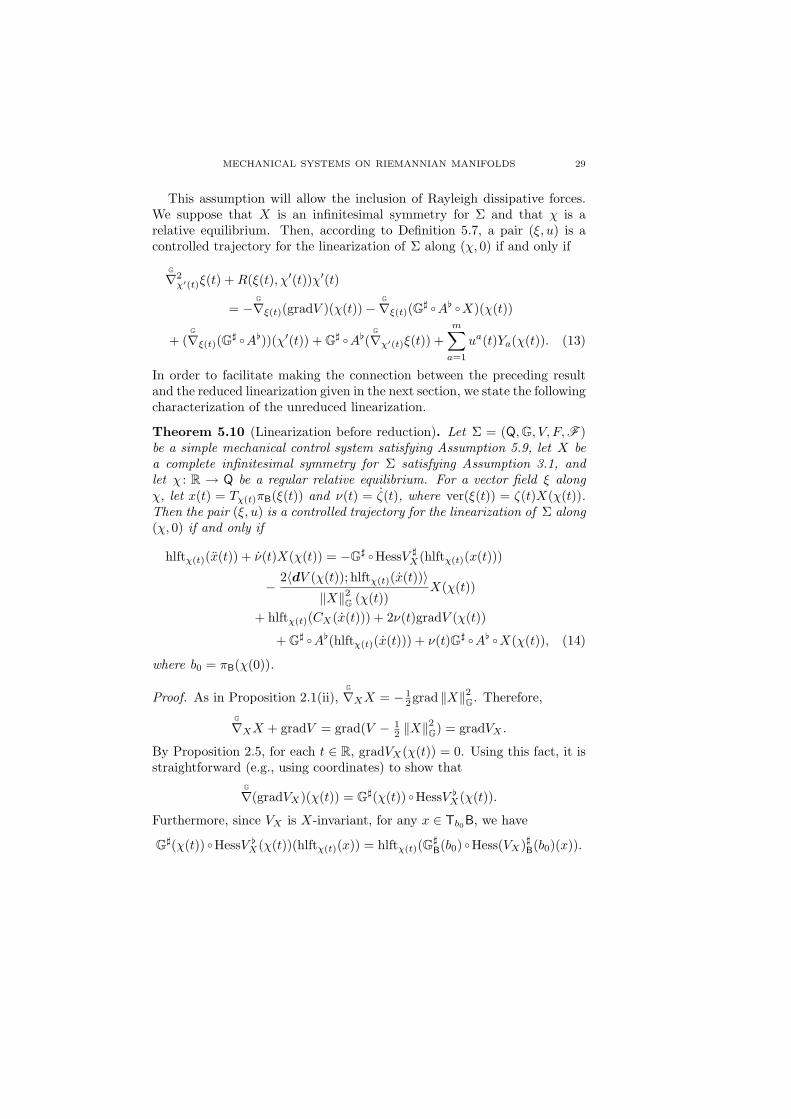
MECHANICAL SYSTEMS ON RIEMANNIAN MANIFOLDS 29
This assumption will allow the inclusion of Rayleigh dissipative forces.We suppose that X is an infinitesimal symmetry for Σ and that χ is arelative equilibrium. Then, according to Definition 5.7, a pair (ξ, u) is acontrolled trajectory for the linearization of Σ along (χ, 0) if and only if
G∇2
χ′(t)ξ(t) + R(ξ(t), χ′(t))χ′(t)
= −G∇ξ(t)(gradV )(χ(t))−
G∇ξ(t)(G] ◦A[ ◦X)(χ(t))
+ (G∇ξ(t)(G] ◦A[))(χ′(t)) +G] ◦A[(
G∇χ′(t)ξ(t)) +
m∑a=1
ua(t)Ya(χ(t)). (13)
In order to facilitate making the connection between the preceding resultand the reduced linearization given in the next section, we state the followingcharacterization of the unreduced linearization.
Theorem 5.10 (Linearization before reduction). Let Σ = (Q,G, V, F, F )be a simple mechanical control system satisfying Assumption 5.9, let X bea complete infinitesimal symmetry for Σ satisfying Assumption 3.1, andlet χ : R → Q be a regular relative equilibrium. For a vector field ξ alongχ, let x(t) = Tχ(t)πB(ξ(t)) and ν(t) = ζ(t), where ver(ξ(t)) = ζ(t)X(χ(t)).Then the pair (ξ, u) is a controlled trajectory for the linearization of Σ along(χ, 0) if and only if
hlftχ(t)(x(t)) + ν(t)X(χ(t)) = −G] ◦HessV ]X(hlftχ(t)(x(t)))
− 2〈dV (χ(t)); hlftχ(t)(x(t))〉‖X‖2G (χ(t))
X(χ(t))
+ hlftχ(t)(CX(x(t))) + 2ν(t)gradV (χ(t))
+G] ◦A[(hlftχ(t)(x(t))) + ν(t)G] ◦A[ ◦X(χ(t)), (14)
where b0 = πB(χ(0)).
Proof. As in Proposition 2.1(ii),G∇XX = − 1
2grad ‖X‖2G. Therefore,G∇XX + gradV = grad(V − 1
2 ‖X‖2G) = gradVX .
By Proposition 2.5, for each t ∈ R, gradVX(χ(t)) = 0. Using this fact, it isstraightforward (e.g., using coordinates) to show that
G∇(gradVX)(χ(t)) = G](χ(t)) ◦HessV [
X(χ(t)).
Furthermore, since VX is X-invariant, for any x ∈ Tb0B, we have
G](χ(t)) ◦HessV [X(χ(t))(hlftχ(t)(x)) = hlftχ(t)(G]
B(b0) ◦Hess(VX)]B(b0)(x)).
30 FRANCESCO BULLO AND ANDREW D. LEWIS
For a vertical tangent vector vχ(t) ∈ Vχ(t)Q we have
G∇(gradVX)(vχ(t)) = 0,
using the fact that gradVX(χ(t)) = 0 and using X-invariance of VX . Sum-marizing the preceding computations is the following formula for a vectorfield ξ along χ:
G∇(
G∇XX + gradV )(ξ(t)) = hlftχ(t)
(G]
B(b0) ◦Hess(VX)[B(b0)(TπB(ξ(t)))
).
(15)Now let ξ be a vector field along χ and let Ξ be a vector field extending ξ.
Since X(χ(t)) = χ′(t), we have, using the definition of the curvature tensor,
G∇2
χ′(t)ξ(t) + R(ξ(t), χ′(t))χ′(t)
=G∇X
G∇XΞ(χ(t)) +
G∇Ξ
G∇XX(χ(t))−
G∇X
G∇ΞX(χ(t))−
G∇[Ξ,X]X(χ(t)).
A straightforward manipulation, using the fact thatG∇ has zero torsion,
gives
G∇X
G∇XΞ +
G∇Ξ
G∇XX−
G∇X
G∇ΞX −
G∇[Ξ,X]X =
=G∇Ξ
G∇XX + 2
G∇[X,Ξ]X + [X, [X, Ξ]]. (16)
Around a point χ(t0) ∈ image(χ), let (U , φ) be a chart with coordinates(q1, . . . , qn) having the following properties:
(1) X = ∂∂qn ;
(2) ((q1, . . . , qn−1), (qn)) are fiber bundle coordinates for πB : Q → B;(3) for any point χ(t) ∈ U , the basis { ∂
∂q1 (χ(t)), . . . , ∂∂qn (χ(t))} for
Tχ(t)Q is G-orthogonal.
In these coordinates one readily determines that
[X, Ξ](χ(t)) = ξi(t)∂
∂qi, [X, [X, Ξ]](χ(t)) = ξi(t)
∂
∂qi(17)
for all values of t for which χ(t) ∈ U . In these coordinates it also holds that
hlftχ(t)∂
∂qa(b0) =
∂
∂qa(χ(t)), a ∈ {1, . . . , n− 1}. (18)
MECHANICAL SYSTEMS ON RIEMANNIAN MANIFOLDS 31
Therefore, if ξ is as above and if x(t) = TπB(ξ(t)), then we have
2G∇X([X, Ξ](χ(t))) = 2
( G∇hlftχ(t)(x(t))X(χ(t)))
+ 2G∇X(ver([X, Ξ])(χ(t)))
= − hlftχ(t)(CX(x(t))) + 2ver(G∇X(hlftχ(t)(x(t))))
+ 2G∇X(ver([X, Ξ])(χ(t)))
= − hlftχ(t)(CX(x(t))) + 2G∇X(ver([X, Ξ])(χ(t)))
+2X(χ(t))‖X‖2G (χ(t))
G(G∇X(hlftχ(t)(x(t))), X(χ(t)))
= − hlftχ(t)(CX(x(t))) + 2G∇X(ver([X, Ξ])(χ(t)))
− 2X(χ(t))‖X‖2G (χ(t))
G(G∇XX(χ(t)), hlftχ(t)(x(t)))
= − hlftχ(t)(CX(x(t))) + 2G∇X(ver([X, Ξ])(χ(t)))
+2X(χ(t))‖X‖2G (χ(t))
〈dV (χ(t)); hlftχ(t)(x(t))〉, (19)
using the fact thatG∇XX = gradVX − gradV , and that dVX(χ(t)) = 0 for
all t ∈ R. Also,
hlftχ(t)(x(t)) = hor([X, [X, Ξ]](χ(t))), t ∈ R. (20)
In the coordinates (q1, . . . , qn), one also computesG∇X =
GΓi
nj
∂
∂qi⊗ dqj ,
from which we ascertain that
2G∇X(ver([X, Ξ])(χ(t))) = 2
GΓi
nnξn ∂
∂qi,
where no summation is intended over the index “n.” One readily verifiesthat, in our coordinates,
GΓi
nn
∂
∂qi=
G∇XX = gradVX − gradV.
Since dVX(χ(t)) = 0, we have
2G∇X(ver([X, Ξ])(χ(t))) = −2ver([X, Ξ](χ(t)))gradV (χ(t)). (21)
We also clearly have, by definition of L X,χ,
ξn(t)∂
∂qn= ver(L X,χ(ξ(t))), (22)

32 FRANCESCO BULLO AND ANDREW D. LEWIS
where no summation is intended over “n.”To simplify the terms involving the external force, we note that
G∇ξ(t)(G] ◦A[(X(χ(t)))) =
= (G∇ξ(t)(G] ◦A[))(X(χ(t))) +G] ◦A[(
G∇ξ(t)X(χ(t))).
Thus, using the fact thatG∇ is torsion-free, we have
−G∇ξ(t)(G] ◦A[ ◦X)(χ(t)) + (
G∇ξ(t)(G] ◦A[))(χ′(t))
+G] ◦A[(G∇χ′(t)ξ(t)) = G] ◦A[([X, Ξ](χ(t))).
Using (17) and (18) we arrive at
−G∇ξ(t)(G] ◦A[ ◦X)(χ(t)) + (
G∇ξ(t)(G] ◦A[))(χ′(t))
+G] ◦A[(G∇χ′(t)ξ(t)) = G] ◦A[(hlftχ(t)(x(t))) + ξnG] ◦A[(X(χ(t))), (23)
where x(t) = Tχ(t)πB(ξ(t)).Finally, for a vector field ξ along χ, let x(t) = TπB(ξ(t)) and let
ν(t)X(t) = ver(L X,χ(ξ)). In terms of our coordinates above, ν(t) = ξn(t).One now combines equations (15), (16), (17), (19), (20), (21), (22) and (23)to get the result. ¤
Remark 5.11. The preceding theorem is not obvious; in particular, theequivalence of equations (13) and (14) is not transparent. Indeed, the rela-tionship between the curvature tensor and the components of the system thatappear in the theorem statement, C, Hess(VX), and gradV , is rather subtle.In this respect, the proof of the theorem bears study, if these relationshipsare to be understood. •
5.4. Linearization of the reduced equations along a relative equi-librium. We again consider a forced simple mechanical control systemΣ = (Q,G, V, F, F ) satisfying Assumption 5.9, take X to be a completeinfinitesimal symmetry for Σ satisfying Assumption 3.1, and let χ be a rel-ative equilibrium. In this section we provide the form of the linearizationalong a relative equilibrium by linearizing, in the usual manner, the reduced

MECHANICAL SYSTEMS ON RIEMANNIAN MANIFOLDS 33
equations, which we reproduce here for convenience:
GB∇η′(t)η′(t) = −gradB
(V eff
X,v(t)
)B(η(t)) + v(t)CX(η′(t))
+ TπB ◦G] ◦A[(γ′(t)−X(γ(t))
)+ YB,u(t, η(t)),
v(t) = −v(t)〈d(‖X‖2G)B(η(t)); η′(t)〉(‖X‖2G)B(η(t))
+〈A[(γ′(t)−X(γ(t)));X(γ(t))〉
(‖X‖2G)B(η(t))
+G(Yu(t, γ(t)), X(γ(t)))
(‖X‖2G)B(η(t)).
(24)Here (γ, u) is a controlled trajectory for Σ, η = πB ◦γ, and v is defined byver(γ′(t)) = v(t)X(γ(t)).
The reduced equations are straightforward to linearize, since we aremerely linearizing about an equilibrium point. To compactly state the formof the linearization requires some notation. Define a (1, 1)-tensor field AB
on B by
AB(vb) = TqπB ◦G](q) ◦A[(q) ◦hlftq(vb),
for q ∈ π−1B (b). This definition can be shown to be independent of the choice
of q ∈ π−1B (b) by virtue of the X-invariance of A. Define a vector field aB
on B by
aB(b) = TqπB ◦G](q) ◦A[(q)(X(q)),
where q ∈ π−1B (b), and again this definition can be shown to be well-defined.
Finally, define a one-form αB on B by
〈αB(b); vb〉 =〈A[(hlftq(vb)); X(q)〉
(‖X‖2G)B(b),
where q ∈ π−1B (b) and vb ∈ TbB. This definition, too, is independent of the
choice of q.We may now state the form of the linearization of the reduced equations.
The proof of the following result is by fairly simple direct computation.
Proposition 5.12 (Linearization after reduction). Let Σ = (Q,G, V, F, F )be a forced simple mechanical control system, let X be a complete infini-tesimal symmetry of Σ satisfying Assumption 3.1, and let χ be a regularrelative equilibrium with b0 = πB ◦χ(0).
34 FRANCESCO BULLO AND ANDREW D. LEWIS
The linearization of equations (24) about (0b0 , 1) is the linear controlsystem (Tb0B⊕ Tb0B⊕ R, AΣ(b0), BΣ(b0)), where
AΣ(b0) =
0 idTb0B
−GB(b0)] ◦Hess(VX)B(b0)[ CX(b0) + AB(b0)0 −2 dVB(b0)
(‖X‖2G)B(b0)+ αB(b0)
02gradBVB(b0) + aB(b0)
〈A[(X(q0));X(q0)〉(‖X‖2G)B(b0)
,
BΣ(b0) =
0BΣ,2(b0)BΣ,3(b0)
,
where BΣ,2(b0) ∈ L(Rm; Tb0B) is defined by
BΣ,2(b0)(u) =m∑
a=1
uaYB,a(b0),
and where BΣ,3(b0) ∈ L(Rm;R) is defined by
BΣ,3(b0)(u) =m∑
a=1
uaG(Ya(χ(0)), X(χ(0)))(‖X‖2G)B(b0)
.
The equations governing controlled trajectories for the linearization ofthe reduced system are
x(t) = −GB(b0)] ◦Hess(VX)B(b0)[(x(t)) + CX(b0)(x(t))
+ 2ν(t)gradBVB(b0) + AB(b0)(x(t)) + ν(t)aB(b0) + BΣ,2(b0) · u(t),
ν(t) = − 2〈dVB(b0); x(t)〉(‖X‖2G)B(b0)
+ αB(b0)(x(t))
+ ν(t)〈A[(X(q0)); X(q0)〉
(‖X‖2G)B(b0)+ BΣ,3(b0) · u(t).
The following result gives the relationship between the reduced and theunreduced linearization.
Theorem 5.13 (Relationship between linearizations). Let Σ =(Q,G, V, F, F ) be a forced simple mechanical control system with F sat-isfying Assumption 5.9, let X be a complete infinitesimal symmetry of Σsatisfying Assumption 3.1, and let χ be a regular relative equilibrium withb0 = πB ◦χ(0).

MECHANICAL SYSTEMS ON RIEMANNIAN MANIFOLDS 35
For a curve t 7→ x(t) ∈ Tb0B, a vector field ξ along χ, a function ν : R→R, and a locally integrable control t 7→ u(t), the following statements areequivalent:
(i) t 7→ (x(t) ⊕ x(t) ⊕ ν(t), u(t)) is a controlled trajectory for thelinearization of the equations (24) about (0b0 , 1), and in turnhor(ξ(t)) = hlftχ(t)(x(t)), and ν(t) = ζ(t), where ver(ξ(t)) =ζ(t)X(χ(t));
(ii) (ξ, u) is a controlled trajectory for the linearization of Σ about(χ, 0), and in turn x(t) = TπB(ξ(t)), and ν(t) = ζ(t), wherever(ξ(t)) = ζ(t)X(χ(t)).
Proof. This follows easily from Theorem 5.10 and Proposition 5.12. ¤
The theorem is an important one, since it will allow us to switch freelybetween the reduced and unreduced linearizations. In some cases, it willbe convenient to think of certain concepts in the unreduced setting, whilecomputations are more easily performed in the reduced setting.
6. Linearized effective energies
In many existing results concerning stability of relative equilibria, a cen-tral role is played by Hessian of the energy. This is a consequence of thefact that definiteness of the Hessian, restricted to certain subspaces, caneasily deliver stability results in various forms. In this section we studythe Hessian of the effective energy for a relative equilibria. In particular,we consider the interplay of the various natural energies with the reduc-tion process and with linearization. Specifically, we spell out the geometryrelating the processes of linearization and reduction.
6.1. Some geometry associated to an infinitesimal isometry. Theutility of the constructions in this section may not be immediately apparent,but will become clear in Proposition 6.6 below.
In this section we let (Q,G) be a Riemannian manifold with X an in-finitesimal isometry satisfying Assumption 3.1. We denote by TTQX therestriction of the vector bundle πTTQ : TTQ → TQ to image(X). ThusTTQX is a vector bundle over image(X) whose fiber at X(q) is TX(q)TQ.We denote this fiber by TTQX,X(q). In like manner, HTQX and VTQX
denote the restrictions of HTQ and TQ, respectively, to image(X). The
Ehresmann connection on πTQ : TQ → Q, defined byG∇ as in Section 4.2,
gives a splitting of each fiber of TTQX as
TTQX,X(q) = HTQX,X(q) ⊕ VTQX,X(q).

36 FRANCESCO BULLO AND ANDREW D. LEWIS
This gives a vector bundle isomorphism σX : TTQX → HTQX ⊕ VTQX .Denote by ΠB : TQ → TQ/R the projection onto the set of XT -orbits. Wedefine φB : TQ → TB× R by
φB(wq) = (TπB(wq), νX(wq)),
where νX(wq) is defined by ver(wq) = νX(wq)X(q). Note thatφB ◦X(q) = (0πB(q), 1). Indeed, one can easily see that φB,X ,φB|image(X) : image(X) → Z(TB) × {1} is a surjective submersion. Wenext define a vector bundle map ψB : TTQ → T(TB × R) over φB byψB = TφB. We denote ψB,X = ψB|TTQX , noting that this is a sur-jective vector bundle map from TTQX to the restricted vector bundleT(TB × R)|(Z(B) × {1}). Next we wish to give a useful description ofthe vector bundle T(TB×R)|(Z(B)×{1}). We think of TB×R as a vectorbundle over B×R, and we let RB×R be the trivial vector bundle (B×R)×Rover B×R. We then note that T0b
TB ' Tb⊕TbB, where the first componentin the direct sum is tangent to Z(TB) (i.e., is horizontal) and the secondcomponent is tangent to TbB (i.e., is vertical). Thus we have a naturalidentification
T(TB× R)|(Z(B)× {1}) ' (TB× R)⊕ (TB× R)⊕ RB×R (25)
of vector bundles over Z(TB) × {1} ' B × {1}. The fiber over (b, 1) isisomorphic to TbB⊕TbB⊕R. We shall implicitly use the identification (25)in the sequel. Next, we define a vector bundle map ιB : HTQ ⊕ VTQ →(TB× R)⊕ (TB× R)⊕ RB×R by
ιB(uvq ⊕ wvq ) =(TqπB(uvq ), TqπB(wvq −
G∇X(uvq )), νX(wvq −
G∇X(uvq ))
).
We then let ιB,X be the restriction of ιB to HTQX ⊕ VTQX .The following result summarizes and ties together the above construc-
tions.
Lemma 6.1. The following statements hold:
(i) σX is a vector bundle isomorphism over idimage(X) from TTQX
to HTQX ⊕ VTQX ;(ii) φB,X is a surjective submersion from image(X) to B× {1};(iii) ψB,X is a surjective vector bundle map over φB,X from TTQX to
(TB× R)⊕ (TB× R)⊕ RB×R;(iv) ιB,X is a surjective vector bundle map over φB,X from HTQX ⊕
VTQX to (TB× R)⊕ (TB× R)⊕ RB×R;

MECHANICAL SYSTEMS ON RIEMANNIAN MANIFOLDS 37
(v) the following diagram commutes:
TTQXσX //
ψB,X ))TTTTTTTTTTTTTTT HTQX ⊕ VTQX
ιB,Xttiiiiiiiiiiiiiiiii
(TB× R)⊕ (TB× R)⊕ RB×R
Proof. This is most easily proved in an appropriate set of coordinates. Takecoordinates (q1, . . . , qn) for Q with the following properties:
(1) X = ∂∂qn ;
(2) for times t for which χ(t) is in the chart domain,{ ∂
∂q1 (χ(t)), . . . , ∂∂qn (χ(t))} is an orthogonal basis for Tχ(t)Q.
This means that (q1, . . . , qn−1) are coordinates for B. These also form,therefore, coordinates for Z(TB) and thus also for Z(TB) × {1}. Since atypical point in image(X) has the form
((q1, . . . , qn), (0, . . . , 0, 1))
in natural coordinates for TQ, we can use (q1, . . . , qn) as coordinates forimage(X). We denote natural coordinates for TTQ by ((q,v), (u, w)). Then(q, u, w) form a set of coordinates for TTQX .
The map φB from TQ to TB× R has the form
((q1, . . . , qn), (v1, . . . , vn)) 7→ ((q1, . . . , qn−1), (v1, . . . , vn−1), vn).
In the coordinates for image(X) and for Z(TB) × {1}, the map φB,X hasthe form
(q1, . . . , qn) 7→ (q1, . . . , qn−1).
The coordinate form of ψB is then
(((q1, . . . , qn), (v1, . . . , vn)), ((u1, . . . , un), (w1, . . . , wn)))
7→ (((q1, . . . , qn−1), (v1, . . . , vn−1), vn), ((u1, . . . , un−1), (w1, . . . , wn−1), wn))
and the coordinate form for ψB,X is given by
((q1, . . . , qn), (u1, . . . , un), (w1, . . . , wn))
7→ ((q1, . . . , qn−1), (u1, . . . , un−1), (w1, . . . , wn−1), wn). (26)
In coordinates, the map σX is given by
((q1, . . . , qn), (u1, . . . , un), (w1, . . . , wn))
7→ ((q1, . . . , qn), (u1, . . . , un), (w1 +GΓi
njuj , . . . , wn +
GΓn
njuj)).

38 FRANCESCO BULLO AND ANDREW D. LEWIS
Finally, in our above coordinates, the form of the map ιB,X is
((q1, . . . , qn), (u1, . . . , un), (w1, . . . , wn))
7→ ((q1, . . . , qn−1), (u1, . . . , un), (w1−GΓ1
njuj, . . . , wn−1−
GΓn−1
nj wj), wn−GΓn
njuj).
All statements in the statement of the lemma follow directly from the pre-ceding coordinate computations. ¤
We shall see in Proposition 6.6 that ιB,X relates two natural energiesassociated to a relative equilibrium.
6.2. The effective energies and their linearizations. We let Σ =(Q,G, V, F ) be a simple mechanical system with X a complete infinitesimalsymmetry for Σ satisfying Assumption 3.1. First recall from Lemma 2.4 thatthe effective energy for a forced simple mechanical system Σ = (Q,G, V, F )with complete infinitesimal symmetry X is
EX(vq) = 12 ‖vq −X(q)‖2G + VX(q),
where VX = V − 12 ‖X‖2G is the effective potential. The relative equilibria for
Σ are then characterized by the critical points of EX , as in Proposition 2.5.As we shall see in Section 7, the Hessian of the effective energy at suchcritical points is useful for determining the stability of the correspondingrelative equilibrium. The following result characterizes this Hessian in termsof the splitting of the fibers of TTQ using the Ehresmann connection on
πTTQ : TTQ → TQ associated withG∇.
Lemma 6.2. Let Σ = (Q,G, V, F ) be a forced simple mechanical systemand let X be a complete infinitesimal symmetry for Σ. Let vq be a criticalpoint for the effective energy and let TqQ⊕ TqQ be the splitting of TvqTQ
associated withG∇, as described in Section 4.2. Then
HessEX(u1 ⊕ w1, u2 ⊕ w2) =
= G(w1 −G∇u1X(q), w2 −
G∇u2X(q)) + HessVX(u1, u2).
Proof. This is a messy, but straightforward, proof in coordinates. ¤
With this as background, we make the following definition, recalling thenotation uvq ⊕ wvq to denote a point in TvqTQ relative to the splitting
defined byG∇.
Definition 6.3 (Linearized effective energy). Let Σ = (Q,G, V, F ) be aforced simple mechanical system, let X be a complete infinitesimal isometry

MECHANICAL SYSTEMS ON RIEMANNIAN MANIFOLDS 39
for Σ, and let χ be a relative equilibrium. The linearized effective energyis the function on TTQ|image(χ′) defined by
Eχ(uvq ⊕ wvq ) = 12‖wvq −
G∇uvq
X‖2G + 12HessVX(uvq , uvq ),
where vq = χ′(0). •Next we consider the linearized effective energy, but now for the reduced
system. To do so, we assume that πB : Q → B is a surjective submersion,as in Assumption 3.1. The effective energy EX is X-invariant and so dropsto TQ/R ' TB × R. We may further explicitly computed this “reducedeffective energy,” denoted by Ered
X , as
EredX (wb, v) = 1
2GB(wb, wb) + (VX)B(b) + 12 (‖X‖2G)B(b)(v − 1)2.
It then makes sense that the “reduced linearized effective energy” shouldbe the Hessian of this function at a critical point, which corresponds, as wehave seen, to a relative equilibrium. The following result records the formof the Hessian.
Lemma 6.4. Let Σ = (Q,G, V, F ) be a forced simple mechanical system, letX be a complete infinitesimal symmetry for Σ satisfying Assumption 3.1,and let (0b, 1) ∈ TB× R be a critical point for (EX)TB×R. Then
HessEredX (0b, 1)(u1 ⊕ v1 ⊕ ν1, u2 ⊕ v2 ⊕ ν2)
= GB(b)(v1, v2) + Hess(VX)B(b)(u1, u2) + (‖X‖2G)B(b)ν1ν2.
Proof. This is a straightforward computation. ¤
Based on this computation, let us make the following definition.
Definition 6.5 (Reduced linearized effective energy). Let Σ = (Q,G, V, F )be a forced simple mechanical system, let X be a complete infinitesimalisometry for Σ satisfying Assumption 3.1, and let b0 = πB(χ(0)). Thereduced linearized effective energy is the function on Tb0B⊕Tb0B⊕Rdefined by
Eredχ (ub0 , vb0 , ν) = 1
2 ‖vb0‖2GB+ 1
2Hess(VX)B(b0)(ub0 , ub0)+ 12 (‖X‖2G)B(b0)ν2.
•The preceding definition of the reduced linearized effective energy is ob-
tained by “reducing” the effective energy, and then “linearizing” it. Itshould be possible to perform the operations in the opposite order to getto the same answer. To do this explicitly, we use the constructions of thepreceding section. In particular, we use the vector bundle map ιB,X . As thefollowing result indicates, one should think of this map as describing how
40 FRANCESCO BULLO AND ANDREW D. LEWIS
the process of linearization is reduced when using the Ehresmann connection
on πTTQ : TTQ → TQ associated withG∇.
Proposition 6.6 (Relating the linearized effective energies). Let Σ =(Q,G, V, F ) be a forced simple mechanical system with X a complete infini-tesimal symmetry satisfying Assumption 3.1. If χ is a relative equilibrium,then ιB,X(χ′(t))∗Ered
χ = Eχ for all t ∈ R.
Proof. Let q = χ(t) and let b = πB(q). We compute
ιB,X(χ′(t))∗Eredχ (uvq
⊕ wvq) =
= 12‖TqπB(wvq
−G∇X(uvq
))‖2GB+ 1
2 (‖X‖2G)BνX(wvq−
G∇X(uq))2 +
+ 12Hess(VX)B(b)(TqπB(ub), TqπB(ub))
= 12‖hor(wvq
−G∇X(uvq
))‖2G + ‖ver(wvq−
G∇X(uvq
))‖2G +
+ 12HessVX(q)(uvq , uvq ),
as desired. ¤
7. Stability of relative equilibria
In this section we apply the results of the preceding sections to study thestability of a relative equilibrium. We deal with stability in two ways: linearand nonlinear. Because we use the linearized effective energy as a Lyapunovfunction in our linear stability analysis, if the conditions we give for linearstability are satisfied, then one can conclude nonlinear stability as well.
7.1. Nonlinear stability definitions. Let us establish the basic setupfor all the following definitions and results. We consider a forced simplemechanical system Σ = (Q,G, V, F ) with a time-independent external forceF and with the following governing equation:
G∇γ′(t)γ
′(t) = −gradV (γ(t)) +G](F (γ′(t))). (27)
We assume for simplicity that all solutions to this equation can be definedon all of R.
Let us define the notions of stability for relative equilibria that we con-sider in this paper.
Definition 7.1 (Base and fiber stability). Let X be a complete infinitesimalsymmetry for Σ, let χ : R → Q be a regular relative equilibrium, and letb0 = πB(χ(0)).

MECHANICAL SYSTEMS ON RIEMANNIAN MANIFOLDS 41
(i) The relative equilibrium χ is base stable if, for all neighborhoodsU of 0b0 , there exists a neighborhood W of χ′(0) such that eachsolution γ : R→ Q of equation (27), with initial condition γ′(0) ∈W, satisfies TπB ◦γ′(t) ∈ U for all t ∈ R.
(ii) The relative equilibrium χ is locally asymptotically base stableif it is base stable, and if there exists a neighborhood V of χ′(0)such that each solution γ : R → Q of equation (27), with initialcondition γ′(0) ∈ V, satisfies limt→+∞ TπB ◦γ′(t) = 0b0 .
(iii) The relative equilibrium χ is fiber stable if, for all neighborhoodsUR of 1, there exists a neighborhood W of χ′(0) such that eachsolution γ : R→ Q of equation (27), with initial condition γ′(0) ∈W, satisfies JX(γ′(t)) ‖X‖−2
G (γ(t)) ∈ UR for all t ∈ R.(iv) The relative equilibrium χ is locally asymptotically fiber stable
if it is fiber stable, and if there exists a neighborhood V of χ′(0)such that each solution γ : R → Q of equation (27), with initialcondition γ′(0) ∈ V, satisfies limt→+∞ JX(γ′(t)) ‖X‖−2
G (γ(t)) =1. •
To describe base stability, consider an invariant tube around the regularrelative equilibrium χ. Base stability means that trajectories starting in thetube remain in the tube at subsequent times; see Figure 3. Fiber stabilitymeans that trajectories starting with nearby initial velocities will maintainnearby fiber velocities at subsequent times. Even if a system is base andfiber stable, trajectories with nearby initial conditions may diverge.
What we call base stability of a relative equilibrium corresponds to theusual notion of stability for a relative equilibrium considered in the litera-ture: stability of the equilibrium point in the reduced space. What we callfiber stability has to do, note, with only the velocity along the fiber. Thusfiber stability will generally not suffice to give other forms of stability alongthe relative equilibrium, such as the G-stability of Patrick [1992]. We alsoremark that the definitions of base and fiber stability are examples of whatis sometimes called “partial stability” in more general contexts. With thissort of stability, one is only interested in the behavior of some of the statesof the system. This is studied in the text [Vorotnikov 1998].
7.2. Linear stability definitions. We let Σ = (Q,G, V, F ) be a forcedsimple mechanical system where the force F satisfies Assumption 5.9, withX a complete infinitesimal symmetry for the system, and with χ : R → Qa relative equilibrium. First we need a definition for linear stability of arelative equilibrium. The definition relies on the linearization along therelative equilibrium, which, from the developments of Section 5, satisfies an

42 FRANCESCO BULLO AND ANDREW D. LEWIS
Q
π−1
B(U)
πB
B( )
U
b0
Figure 3. Base stability of relative equilibria
initial value problem of the formG∇2
χ′(t)ξ(t) + R(ξ(t), χ′(t))χ′(t)
= −G∇ξ(t)(gradV )(χ(t))−
G∇ξ(t)(G] ◦A[ ◦X)(χ(t))
+ (G∇ξ(t)(G] ◦A[))(χ′(t)) +G] ◦A[(
G∇χ′(t)ξ(t)),
ξ(0) = ξ0, L X,χ(ξ)(0) = vξ,0. (28)
Remarks 7.2. (1) Note that it is immaterial that we specify the initialcondition at t = 0 due to X-invariance of the system.
(2) Also note that we can specify the initial derivative condition for ξ
by specifyingG∇χ′(0)ξ(0). Since both L X,χ and
G∇χ′ are differential
operators in TQ along χ, L X,χ(ξ)(t) −G∇χ′(t)ξ(t) depends only on
ξ(t). Thus specifying ξ(0) and L X,χ(ξ)(0) is equivalent to specifying
ξ(0) andG∇χ′(0)ξ(0). For our purposes, it is more convenient to
specify the derivative initial condition in terms of L X,χ(ξ)(0). •We may now state our stability definitions.
Definition 7.3 (Linear stability of relative equilibria). Let Σ = (Q,G, V, F )be a forced simple mechanical system with F satisfying Assumption 5.9,with X a complete infinitesimal symmetry for Σ, and with χ : R → Q a
MECHANICAL SYSTEMS ON RIEMANNIAN MANIFOLDS 43
relative equilibrium. For a vector field ξ along χ, let ν(t) = ζ(t), wherever(ξ(t)) = ζ(t)X(χ(t)).
(i) The relative equilibrium χ is linearly base (resp. fiber) stableif there exists M > 0 such that the solution t 7→ ξ(t) to the initialvalue problem (28) satisfies ‖hor(ξ(t))‖G+ ‖L X,χ(hor(ξ))(t)‖G ≤M(‖hor(ξ0)‖G+‖vξ,0‖G) (resp. |ν(t)| ≤ M(‖hor(ξ0)‖G+‖vξ,0‖G)).
(ii) The relative equilibrium χ is linearly asymptotically base(resp. fiber) stable if each solution t 7→ ξ(t) to theinitial value problem (28) satisfies limt→+∞(‖hor(ξ(t))‖G +‖L X,χ(hor(ξ))(t)‖G) = 0 (resp. limt→+∞ ν(t) = 0). •
Let us now give the relationship between these definitions of linear stabil-ity and the linear stability of the reduced system. To do this, let us write theequations governing the reduced linearization, following Proposition 5.12:
x(t) = −GB(b0)] ◦Hess(VX)B(b0)[(x(t)) + CX(b0)(x(t))
+ 2ν(t)gradBVB(b0) + FB(b0)(x(t)) + ν(t)fB(b0),
ν(t) = − 2〈dVB(b0); x(t)〉(‖X‖2G)B(b0)
+ αB(b0)(x(t)) + ν(t)〈A[(X(q0));X(q0)〉
(‖X‖2G)B(b0),
(29)
where we adopt the notation for FB, fB, and αB as given before the state-ment of Proposition 5.12. We also let R+ denote the set of nonnegative realnumbers.
Proposition 7.4 (Base characterization of linear stability). Let Σ =(Q,G, V, F ) be a forced simple mechanical system with F satisfying As-sumption 5.9, with X a complete infinitesimal symmetry for the systemsatisfying Assumption 3.1, and with χ : R → Q a regular relative equilib-rium. Let b0 = πB(χ(0)). The following statements hold:
(i) χ is linearly base stable if and only if, for every solution t 7→x(t) ⊕ x(t) ⊕ ν(t) of the equations (29), the function R+ 3 t 7→‖x(t)‖GB(b0)
is bounded;(ii) χ is linearly asymptotically base stable if and only if, for
every solution t 7→ x(t) ⊕ x(t) ⊕ ν(t) of the equations (29),limt→+∞ ‖x(t)‖GB(b0)
= 0;(iii) χ is linearly fiber stable if and only if, for every solution t 7→ x(t)⊕
x(t) ⊕ ν(t) of the equations (29), the function R+ 3 t 7→ |ν(t)| isbounded;
(iv) χ is linearly asymptotically fiber stable if and only if, for every so-lution t 7→ x(t)⊕x(t)⊕ν(t) of the equations (29), limt→+∞ |ν(t)| =0.

44 FRANCESCO BULLO AND ANDREW D. LEWIS
Proof. This is a direct consequence of properties of time-independent lineardifferential equations. ¤
7.3. Lyapunov stability analysis. Next, we endeavor to provide stabilitycriteria for relative equilibria. We start by introducing a few appropriateconcepts.
Let us also introduce the appropriate notions of dissipative forces alonga relative equilibrium.
Definition 7.5. Let X ∈ Γ∞(TQ). A time-independent force F : TQ →T∗Q is dissipative about X if 〈F (vq); vq −X(q)〉 ≤ 0 for each vq ∈ TQ,and is strictly dissipative about X if it is dissipative about X, and if〈F (vq); vq −X(q)〉 = 0 only when vq = X(q). •
We can now collect some basic statements about these concepts.
Lemma 7.6. Consider the forced simple mechanical system (Q,G, V, F )with infinitesimal symmetry X. If F is dissipative about X, and if γ : I → Qis a trajectory of equation (27), then the function t 7→ EX(γ′(t)) is nonin-creasing.
Proof. Recall that the vector field on TQ describing the dynamics
of (Q,G, V, F ) isGS − vlft(gradV ) + vlft(G] ◦F ). Because EX is a constant
of motion for (Q,G, V ), we know that
L GS−vlft(gradV )
EX = 0.
Next, from Lemma 2.4 we compute
L vlft(G] ◦F )EX(vq) = 〈F (vq); vq −X(q)〉 ≤ 0. (30)
¤
Finally, we can provide criteria for the stability of relative equilibria interms of the character of VX at critical points. These results parallel thosepresented for equilibrium configurations for equilibria of mechanical systems(see, for example, [Bullo and Lewis 2004, Theorem 6.45]). Recall that, underAssumption 3.1, (VX)B is the projection of VX onto the base space B.
Theorem 7.7 (Stability of relative equilibria). Consider a forced simplemechanical system Σ = (Q,G, V, F ) and let X be a complete infinitesimalsymmetry for Σ satisfying Assumption 3.1. Assume F is dissipative about Xand assume F (X(q)) = 0q for each q ∈ Q. Then the following statementshold.
(i) A regular relative equilibrium χ : R→ Q is base and fiber stable if(VX)B is locally positive-definite about πB(χ(0)).

MECHANICAL SYSTEMS ON RIEMANNIAN MANIFOLDS 45
(ii) A regular relative equilibrium χ is locally asymptotically base stableand locally asymptotically fiber stable if (VX)B has an isolated localminimum at πB(χ(0)), and if F is strictly dissipative about X.
Proof. To prove parts (i) and (ii), we use the regularity of the relative equi-librium χ to invoke Theorem 3.3. We recall the equivalent representation ofthe dynamics of Σ obtained in Theorem 3.3(ii). If γ : R → Q is a solutionto (27), then the curve η = πB ◦γ : R → B, and the curve v : R → R givenby v(t) = JX(γ′(t)) ‖X‖−2
G (γ(t)), together satisfy
GB∇η′(t)η′(t)=−gradB
(V eff
X,v(t)
)B(η(t)) + v(t)CX(η′(t))+TπB
(G] ◦F (γ′(t))
),
v(t) = −v(t)〈d(‖X‖2G)B(η(t)); η′(t)〉(‖X‖2G)B(η(t))
+1
(‖X‖2G)B(η(t))〈F (γ′(t)); X(γ(t))〉 .
(31)From the curves η and v, the curve γ : R → Q is computed to be γ(t) =ΦvX
0,t (hlftq0(η)(t)).Let ΣTB×R be reduced dynamical system on TB × R defined by equa-
tions (31). Given this characterization, the curve χ : R → Q is a relativeequilibrium for Σ if and only if its projection t 7→ (πB(χ(0)), 1) is a solutionto equations (31); that is, an equilibrium point for ΣTB×R.
Now we note that EX is a function invariant under the flow of XT .Therefore, EX can be projected onto the reduced space TB×R. Given thedecomposition TQ = HQ⊕VQ, we write vq ∈ TQ as vq = hlftq(wb)+νX(q)for (wb, ν) ∈ TB× R. Accordingly
(EX)TB×R(wb, ν) = EX(hlftq(wb) + νX(q))
= (VX)B(b) + 12GB(wb, wb) + 1
2 (‖X‖2G)B(b)(ν − 1)2.
Because EX is a nonincreasing function along the trajectories of Σ, its pro-jection (EX)TB×R(wb, ν) is a nonincreasing function along the trajectoriesof ΣTB×R. If (VX)B is locally positive-definite about πB(χ(0)), then
(wb, ν) 7→ (EX)TB×R(wb, ν)− VX(χ(0))
is a Lyapunov function for the dynamical system ΣTB×R about the point(0πB(χ(0)), 1) ∈ TB×R. This proves part (i), that is, the relative equilibriumχ : R→ Q is base and fiber stable.
To prove (ii), we invoke the LaSalle Invariance Principle for the dynamicalsystem ΣTB×R. We now assume that F is strictly dissipative about Xand recall that F is X-invariant. Since πB(χ(0)) ∈ B is an isolated localminimum for
(VX
)B, there exists a neighborhood W ⊂ B of πB(χ(0)) such
that(VX
)B(b) >
(VX
)B(b0) for all b ∈ W \ {πB(χ(0))}, and W contains no

46 FRANCESCO BULLO AND ANDREW D. LEWIS
critical point other than πB(χ(0)). Next, we compute
A = { (wb, ν) ∈ TW × R| 〈F (vq); vq〉 = 0 for vq = hlftq(wb) + νX(q)}= { (wb, ν) ∈ TW × R| vq = X(q) for vq = hlftq(wb) + νX(q)}= {(0b, 1) ∈ TW × R}.
On A, the equations (31) reduce to 0 = −gradB
(VX
)B(η). Therefore, no
trajectory of (31) takes values in A, other than the trivial t 7→ (πB(χ(0)), 1).Under these conditions, the LaSalle Invariance Principle guarantees that(πB(χ(0)), 1) is locally asymptotically stable. ¤ ¤
Theorem 7.7(i) can be stated directly in terms of the effective potentialfunction rather than in terms of its projection. The helpful equivalence isstated as follows.
Lemma 7.8. Let X ∈ Γ∞(TQ) satisfy Assumption 3.1. Let ψ ∈ C∞(Q) beX-invariant and let ψ(q0) = 0 for q0 ∈ Q. Then the following statementsare true:
(i) πB(q0) is a critical point for ψB if and only if q0 is a critical pointfor ψ;
(ii) ψB is locally positive-definite about πB(q0) if and only if there existsa neighborhood W of q0 with the properties that
(a) q ∈ W implies ψ(q) ≥ 0, and(b) ψ(q) = 0 only if q belongs to the integral curve of X
through q0;(iii) if q0 is a critical point for ψ, then HessψB(πB(q0)) is positive-
definite if and only if Hessψ(q0) is positive-definite on any com-plement to spanR {X(q0)} in Tq0Q.
Proof. There exists a chart (U , φ) with coordinates (q1, . . . , qn), withφ(q0) = 0, and X = ∂
∂q1 . Because ψ is X-invariant, the coordinate rep-resentation of ψ does not depend on q1 and therefore its Taylor expansionis
ψ(q1, . . . , qn) ==
∑ni=2(dψ(q0))iq
i + 12
∑ni,j=2(Hessψ(q0))ijq
iqj + O(‖(q1, . . . , qn)‖3Rn
).
The integral curve of X through q0 is an open subset of theaxis
{(q1, 0, . . . , 0)
∣∣ q1 ∈ R}, and by construction ψB(q2, . . . , qn) =
ψ(0, q2, . . . , qn). Statements (i) and (ii) are consequences of these facts.Part (iii) follows by noting that Hessψ(q0) is positive-definite on any com-plement to spanR {(1, 0, . . . , 0)} if and only if the (n− 1) eigenvalues of the(n − 1) × (n − 1) matrix with components (Hessψ(q0))ij , i, j ∈ {2, . . . , n},are strictly positive. ¤
MECHANICAL SYSTEMS ON RIEMANNIAN MANIFOLDS 47
Remarks 7.9. (1) Effective versus amended potential functions:Proposition 2.5 and Theorem 7.7(i) can be stated in terms of theamended potential function instead of the effective potential func-tion (see [Bullo and Lewis 2004, Exercise 6.20]). For part (ii), itis convenient to rely on the effective potential function rather thanthe amended potential function.
(2) Similarities with equilibrium configurations: The results of Theo-rem 7.7 are similar to those characterizing the existence and stabilityof equilibrium configurations. Roughly speaking, the effective energyplays the same role in analyzing a relative equilibria as the energyfunction plays in analyzing equilibrium configurations (cf. [Bulloand Lewis 2004, Theorem 6.45]). In the study of relative equilib-ria, the effective potential function plays a role parallel to the oneplayed by the potential function in the study of equilibrium configu-rations. Furthermore, the second term in Lemma 2.4 characterizingthe effective energy is a positive-definite function in the “velocityerror” (vq −X(q)).
(3) Comparison with the Energy-Momentum Method: The stabilitycriterion in Theorem 7.7 is only sufficient: it turns out that,because of the Noether Conservation Law, it is not necessaryto require positive-definitness of HessVX on every complement tospanR {X(q0)} in Tq0Q. The Energy-Momentum Method describedin [Marsden 1992, Marsden and Ratiu 1999, Simo, Lewis, andMarsden 1991] provides a sharper, more detailed analysis by tak-ing this into account. •
7.4. Linear stability analysis. Now let us give some natural sufficientconditions that rely only on the linearization. These conditions should bethought of as the linear analogue to the stability results of the precedingsection. As such, they use the notions of linearized effective energies fromSection 6.2. In this regard, the next result is the main result in this section.
Theorem 7.10 (Linear stability of relative equilibria). Let Σ =(Q,G, V, F ) be a forced simple mechanical system, with X a complete in-finitesimal symmetry for Σ satisfying Assumption 3.1, and with χ : R→ Qa regular relative equilibrium. Suppose that F (vq) = −R[
diss(vq − X(q)),where Rdiss is a symmetric positive-semidefinite (0, 2)-tensor field. Forb0 = πB ◦χ(0), the following statements hold:
(i) χ is linearly base and fiber stable if Hess(VX)B(b0) is positive-definite;
(ii) χ is linearly asymptotically base stable and linearly asymptoticallyfiber stable if Hess(VX)B(b0) is positive-definite and if Rdiss ispositive-definite.

48 FRANCESCO BULLO AND ANDREW D. LEWIS
Proof. Note that combined linear (asymptotic) base and fiber stability of χis equivalent to the linear (asymptotic) stability of the equilibrium point b0
for the reduced system on TB×R. Therefore, in the proof, we shall considerthe stability in the reduced space, using the reduced linearized effectiveenergy, Eref
χ , as a candidate Lyapunov function. First note that, under thehypothesis that Hess(VX)B(b0) is positive-definite, it follows that Eref
χ ispositive-definite about 0b ⊕ 0b ⊕ 0. Next, a straightforward computation,the details of which we omit, shows that
dEredχ
dt(x(t)⊕ x(t)⊕ ν(t)) = GB(x(t), FB(b0)(x(t))) + ν(t)GB(x(t), fB(b0))
+ ν(t)(‖X‖2G)B(b0)αB(b0)(x(t)) + ν(t)2〈A[(X(q0));X(q0)〉,along a solution t 7→ x(t)⊕x(t)⊕ν(t) to equations (29), where q0 ∈ π−1
B (b0),and where A is as in Assumption 5.9. One now can easily show that
GB(x(t), FB(b0)(x(t))) = A(hlftq0(x(t)),hlftq0(x(t))),
ν(t)GB(x(t), fB(b0)) = A(ν(t)X(q0), hlftq0(x(t))),
ν(t)(‖X‖2G)B(b0)αB(b0)(x(t)) = A(hlftq0(x(t)), ν(t)X(q0)).
These computations allow us to conclude that
dEredχ
dt(x(t)⊕ x(t)⊕ ν(t)) =
= A(hlftq0(x(t)) + ν(t)X(q0), hlftq0(x(t)) + ν(t)X(q0)).
In part (i), A = −Rdiss is negative-semidefinite, and in part (ii), A = −Rdiss
is negative-definite, and the result then follows directly. ¤
Alternatively, one can check the hypotheses of the theorem using thelinearized effective energy. The following result contains the results of thistranscription.
Corollary 7.11 (Unreduced linear stability of relative equilibria). LetΣ = (Q,G, V, F ) be a forced simple mechanical system, with X a completeinfinitesimal symmetry for Σ satisfying Assumption 3.1, and with χ : R→ Qa regular relative equilibrium. Suppose that F (vq) = −R[
diss(vq − X(q)),where Rdiss is a Rayleigh dissipation function. The following statementshold:
(i) χ is linearly base and fiber stable if HessVX(χ(t)) is positive-definite on any (and so every) complement to spanR {X(χ(t))}for some (and so for all) t ∈ R;
(ii) χ is linearly asymptotically base stable and linearly asymptoticallyfiber stable if HessVX(χ(t)) is positive-definite on any (and so
MECHANICAL SYSTEMS ON RIEMANNIAN MANIFOLDS 49
every) complement to spanR {X(χ(t))} for some (and so for all)t ∈ R, and if Rdiss is positive-definite.
Remarks 7.12. (1) Note that since positive-definiteness of theHessian of (VX)B at b0 implies that b0 is an isolated local mini-mum for (VX)B, the satisfaction of the hypotheses of Theorem 7.10implies the satisfaction of the hypotheses of Theorem 7.7.
(2) The presence of gyroscopic forces in the reduced linearization makesit difficult to draw the sharpest possible conclusions regarding linearstability. This is to be contrasted with the linear stability of equi-librium points, where it is possible to give much sharper stabilityconditions in the presence of only dissipative forces (see, for exam-ple, [Bullo and Lewis 2004, Theorem 6.42]).
(3) In part (ii) of Theorem 7.10 we require that Rdiss be positive-definite.As is the case with stability of equilibria for mechanical systems, thishypothesis is stronger than required. •
8. Open problems and future directions
We conclude with a discussion of some of the more obvious researchdirections suggested by our approach.
(1) First and foremost, it would be important to analyze the setting ofreduction by a general Lie group action. In such a setup, one mightconsider a principal fiber bundle π : Q → B with structure groupbeing a Lie group G. One would then be interested in the Rie-mannian geometry of the principal bundle. For example, reductionshould be describable in terms of ideas such as the reduced Rie-mannian metric on B, the mechanical connection and its curvature,the locked inertia tensor, the second fundamental form of the fibers,and the amended/effective potential. This picture is only partiallyunderstood at present (but see some initial results in [Cortes andMartınez 2003]), and the application of this picture to stability the-ory is described in [Marsden 1992].
(2) In a related direction, with regards to the stability analysis forrelative equilibria, it would be interesting to describe the Energy-Momentum method of [Simo, Lewis, and Marsden 1991, Simo, Pos-bergh, and Marsden 1990] in Riemannian geometric language.
(3) Generalizing from the Riemannian context, one could study thegeometry of a G-invariant affine connection on a principal fiberbundle π : Q → B. From the point of view of mechanics, this isinteresting since the dynamics of systems with nonholonomic con-straints can be described using an affine connection that is generally

50 FRANCESCO BULLO AND ANDREW D. LEWIS
different from the affine connection. This is an idea that goes backto Synge [1928].
(4) It would also be interesting to characterize the linearization of amechanical control system along more general trajectories than rel-ative equilibria. An interesting example of such trajectories arethose arising in the theory of kinematic reduction for affine con-nection control systems [Bullo and Lewis 2003, Bullo and Lynch2001].
(5) From a control theoretical viewpoint, very little is known about thelinear and nonlinear controllability properties of mechanical controlsystems along relative equilibria. This is due to the complicationsarising from the gyroscopic forces present in the reduced equations.The geometry of the controllability properties of linear mechanicalsystems with gyroscopic forces are not well understood presently,but some results are contained in the paper of Hughes and Skelton[1980].
References
Abraham, R. and Marsden, J. E. [1978] Foundations of Mechanics, secondedition, Addison Wesley, Reading, MA, ISBN 0-8053-0102-X.
Arnol’d, V. I. [1966] Sur la geometrie differentielle des groupes de Lie de di-mension infinie et ses applications a l’hydrodynamique des fluides parfaits,Universite de Grenoble. Annales de l’Institut Fourier, 16(1), 319–361.
Bloch, A. M. [2003] Nonholonomic Mechanics and Control, vol-ume 24 of Interdisciplinary Applied Mathematics, Springer-Verlag, NewYork–Heidelberg–Berlin, ISBN 0-387095535-6.
Bullo, F. [2000] Stabilization of relative equilibria for underactuated sys-tems on Riemannian manifolds, Automatica. The Journal of IFAC. TheInternational Federation of Automatic Control, 36(12), 1819–1834.
Bullo, F. and Lewis, A. D. [2003] Low-order controllability and kinematicreductions for affine connection control systems, SIAM Journal on Controland Optimization, to appear.
— [2004] Geometric Control of Mechanical Systems: Modeling, Analysis,and Design for Simple Mechanical Systems, number 49 in Texts in Ap-plied Mathematics, Springer-Verlag, New York–Heidelberg–Berlin, ISBN0-387-22195-6.
— [2005] Supplementary chapters for Geometric Control of Mechanical Sys-tems [Bullo and Lewis 2004].URL: http://penelope.mast.queensu.ca/smcs/
Bullo, F. and Lynch, K. M. [2001] Kinematic controllability and decou-pled trajectory planning for underactuated mechanical systems, Institute
MECHANICAL SYSTEMS ON RIEMANNIAN MANIFOLDS 51
of Electrical and Electronics Engineers. Transactions on Robotics andAutomation, 17(4), 402–412.
Cendra, H., Marsden, J. E., Pekarsky, S., and Ratiu, T. S. [2003] Variationalprinciples for Lie–Poisson and Hamilton–Poincare equations, MoscowMathematical Journal, 3(3), 833–867.
Cendra, H., Marsden, J. E., and Ratiu, T. S. [2001] Lagrangian reductionby stages, Memoirs of the American Mathematical Society, 152(722).
Cortes, J. and Martınez, S. [2003] Motion control algorithms for simple me-chanical systems with symmetry, Acta Applicandae Mathematicae. AnInternational Journal on Applying Mathematics and Mathematical Ap-plications, 76(3), 221–264.
Crampin, M. and Pirani, F. A. E. [1986] Applicable Differential Geometry,number 59 in London Mathematical Society Lecture Note Series, Cam-bridge University Press, New York/Port Chester/Melbourne/Sydney,ISBN 0-521-23190-6.
Guillemin, V. and Sternberg, S. [1984] Symplectic Techniquesin Physics, Cambridge University Press, New York/PortChester/Melbourne/Sydney, ISBN 0-521-38990-9.
Hughes, P. C. and Skelton, R. E. [1980] Controllability and observabilityof linear matrix-second-order systems, American Society of MechanicalEngineers. Transactions of the ASME. Series E. Journal of Applied Me-chanics, 47(2), 415–420.
Jalnapurkur, S. M. and Marsden, J. E. [2000] Stabilization of relative equi-libria, Institute of Electrical and Electronics Engineers. Transactions onAutomatic Control, 45(8), 1483–1491.
— [2001] Stabilization of relative equilibria. II, Regular & Chaotic Dynam-ics. Regulyarnaya & Khaoticheskaya Dinamika, 3(3), 161–179.
Kobayashi, S. and Nomizu, K. [1963] Foundations of Differential Geometry,Volumes I and II, number 15 in Interscience Tracts in Pure and AppliedMathematics, Interscience Publishers, New York.
Lewis, A. D. and Tyner, D. R. [2003] Jacobian linearisation in a geometricsetting, in Proceedings of the 42nd IEEE Conference on Decision andControl, pages 6084–6089, Maui, HI.
Marsden, J. E. [1992] Lectures on Mechanics, number 174 in London Math-ematical Society Lecture Note Series, Cambridge University Press, NewYork/Port Chester/Melbourne/Sydney, ISBN 0-521-42844-0.
Marsden, J. E. and Ratiu, T. S. [1999] Introduction to Mechanics andSymmetry, second edition, number 17 in Texts in Applied Mathematics,Springer-Verlag, New York–Heidelberg–Berlin, ISBN 0-387-98643-X.
Marsden, J. E. and Weinstein, A. [1974] Reduction of symplectic manifoldswith symmetry, Reports on Mathematical Physics, 5(1), 121–130.

52 FRANCESCO BULLO AND ANDREW D. LEWIS
Meyer, K. R. [1973] Symmetries and integrals in mechanics, in DynamicalSystems, M. Peixoto, editor, pages 259–273, Academic Press, New York.
Ortega, J.-P. and Ratiu, T. S. [2004] Momentum Maps and Hamilton-ian Reduction, number 222 in Progress in Mathematics, Birkhauser,Boston/Basel/Stuttgart, ISBN 0-8176-4307-9.
Patrick, G. W. [1992] Relative equilibria in Hamiltonian systems: the dy-namic interpretation of nonlinear stability on a reduced phase space, Jour-nal of Geometry and Physics, 9(2), 111–119.
Sasaki, S. [1958] On the differential geometry of tangent bundles of Rie-mannian manifolds, The Tohoku Mathematical Journal. Second Series,10, 338–354.
— [1962] On the differential geometry of tangent bundles of Riemannianmanifolds II, The Tohoku Mathematical Journal. Second Series, 14, 146–155.
Simo, J. C., Lewis, D. R., and Marsden, J. E. [1991] Stability of relativeequilibria I: The reduced energy momentum method, Archive for RationalMechanics and Analysis, 115(1), 15–59.
Simo, J. C., Posbergh, T. A., and Marsden, J. E. [1990] Stability of coupledrigid bodies and geometrically exact rods—block diagonalisation and theenergy momentum method, Physics Reports. A Review Section of PhysicsLetters, 193(6), 279–360.
Sussmann, H. J. [1997] An introduction to the coordinate-free maximumprinciple, in Geometry of Feedback and Optimal Control, B. Jakubczykand W. Respondek, editors, pages 463–557, Dekker Marcel Dekker, NewYork.
Synge, J. L. [1928] Geodesics in nonholonomic geometry, MathematischeAnnalen, 99, 738–751.
Vorotnikov, V. I. [1998] Partial Stability and Control, Birkhauser,Boston/Basel/Stuttgart, ISBN 0-8176-3917-9.
Yano, K. and Ishihara, S. [1973] Tangent and Cotangent Bundles, number 16in Pure and Applied Mathematics, Dekker Marcel Dekker, New York,ISBN 0-8247-6071-9.
Francesco BulloAssociate ProfessorMechanical & Environmental Eng.Univ. of California at Santa BarbaraEngineering II Bldg.Santa Barbara, CA 93106-5070, [email protected]
Andrew D. LewisAssociate ProfessorDep. of Math. and StatisticsQueen’s UniversityKingston, ON K7L 3N6, [email protected]
Related Documents