Reduced space optimal interpolation of daily rain gauge precipitation in Switzerland

ClickHere

for

FullArticle

Reduced space optimal interpolation of daily raingauge precipitation in Switzerland

R. Schiemann,1 M. A. Liniger,1 and C. Frei1

Received 21 August 2009; revised 5 March 2010; accepted 22 March 2010; published 22 July 2010.

[1] The coarse spacing of automatic rain gauges complicates near‐real‐time spatialanalyses of precipitation. We test the possibility of improving such analyses byconsidering, in addition to the in situ measurements, the spatial covariance structureinferred from past observations with a denser network. To this end, a statisticalreconstruction technique, reduced space optimal interpolation (RSOI), is applied overSwitzerland, a region of complex topography. RSOI consists of two main parts. First,principal component analysis (PCA) is applied to obtain a reduced space representation ofgridded high‐resolution precipitation fields available for a multiyear calibration period inthe past. Second, sparse real‐time rain gauge observations are used to estimate theprincipal component scores and to reconstruct the precipitation field. In this way,climatological information at higher resolution than the near‐real‐time measurements isincorporated into the spatial analysis. PCA is found to efficiently reduce thedimensionality of the calibration fields, and RSOI is successful despite the difficultiesassociated with the statistical distribution of daily precipitation (skewness, dry days).Examples and a systematic evaluation show substantial added value over a simpleinterpolation technique that uses near‐real‐time observations only. The benefit isparticularly strong for larger‐scale precipitation and prominent topographic effects.Small‐scale precipitation features are reconstructed at a skill comparable to that of thesimple technique. Stratifying the reconstruction method by the types of weather typeclassifications yields little added skill. Apart from application in near real time, RSOI mayalso be valuable for enhancing instrumental precipitation analyses for the historic pastwhen direct observations were sparse.

Citation: Schiemann, R., M. A. Liniger, and C. Frei (2010), Reduced space optimal interpolation of daily rain gaugeprecipitation in Switzerland, J. Geophys. Res., 115, D14109, doi:10.1029/2009JD013047.

1. Introduction

[2] There is an obvious need for quantitative and spatiallyresolved information on precipitation in applications such asrunoff forecasting, water resources management, and ava-lanche warning systems. In Switzerland, the climatologicalrain gauge network is sufficiently dense to meet the require-ments of most applications. Yet, only a rather small part of thegauges can provide measurements on a real‐time basis and inan automated fashion. Most of the observations are takenmanually and typically become available with a delay ofsome days or weeks. Therefore, gridding methods have torely on a coarse network of stations when applied in a real‐time context, which may severely limit the quality ofinterpolated analyses. An example of such a situation isshown in Figure 1. The field in Figure 1a is based on acoarse network. While it can adequately represent the gross

properties of the spatial precipitation distribution, someshortcomings are evident when comparing to a field ob-tained from the full dense network of stations by means ofthe same interpolation method (Figure 1b).[3] Radar measurements are widely used to overcome

these limitations. Indeed, the formal combination of the twodata sources has been shown to provide substantiallyimproved analyses in a number of cases [Seo et al., 1990;Seo, 1998; Todini, 2001; Sinclair and Pegram, 2005;Haberlandt, 2007; DeGaetano and Wilks, 2009; Erdin,2009; Velasco‐Forero et al., 2009]. The strength of theradar is to yield a spatially coherent estimate of the pre-cipitation distribution. The accuracy of this estimate at anygiven point, however, is comparatively low due to technicalproblems associated with ground clutter, beam blocking,and attenuation [e.g., Germann et al., 2006]. These pro-blems are of particular relevance in mountainous terrain.[4] In this study, we investigate an alternative method for

enhancing the near‐real‐time spatial analysis of dailyprecipitation from a sparse gauge network. In addition tothe observations from the sparse network, this methodincorporates information on the spatial covariance in the

1Federal Office of Meteorology and Climatology MeteoSwiss, Zurich,Switzerland.

Copyright 2010 by the American Geophysical Union.0148‐0227/10/2009JD013047

JOURNAL OF GEOPHYSICAL RESEARCH, VOL. 115, D14109, doi:10.1029/2009JD013047, 2010

D14109 1 of 18

daily precipitation fields determined from high‐resolutionmeasurements available in the past. In a mountainous region,precipitation patterns have a strongly convoluted spatialstructure such that network density is a particularly importantcontrol on interpolation skill [e.g., Dorninger et al., 2008;Hofstra et al., 2008]. At the same time, however, precipita-tion patterns are recurrent in time due to a characteristicorographic forcing in situations with similar large‐scaleatmospheric circulation. Consequently, it appears promisingto test our approach for the territory of Switzerland.[5] The method we use is reduced space optimal inter-

polation (RSOI) [Kaplan et al., 1997]. Previous applicationsof this technique have been concerned with the reconstruc-tion of global historical monthly sea surface temperatures,night marine air temperature, and sea ice [Kaplan et al.,1998; Rayner et al., 2003], of monthly marine and globalmean sea level pressure [Kaplan et al., 2000; Allan andAnsell, 2006], of daily mean sea level pressure for theEuropean‐North Atlantic region [Ansell et al., 2006], ofPacific sea surface temperatures from proxy data [Evans etal., 2002], and of monthly precipitation in the Alps[Schmidli et al., 2001, 2002]. To the knowledge of the au-thors, this is the first study to test the feasibility of re-constructing daily, i.e. strongly skewed, precipitation databy means of RSOI. While the above studies are concernedwith the reconstruction of historical climate data, the ideabehind this study is a near‐real‐time application of RSOIwhere the reconstruction period corresponds to a “veryrecent past”.

[6] Several authors have exploited weather type infor-mation for mesoscale precipitation analysis. For example,Courault and Monestiez [1999] have determined weathertype dependent lapse rates and semi‐variograms in anordinary kriging, Tveito [2002] uses a weather type strati-fication in the deterministic component of a griddingscheme, and Hewitson and Crane [2005] have modified theclassical Shepard approach [Shepard, 1968, 1984; Rudolf etal., 1992] by introducing weather type dependent stationweights. Herein, we follow these ideas and stratify RSOIwith respect to the types of two classifications of the cir-culation in Central Europe.[7] The paper is structured as follows: In section 2, the

precipitation data sets and the study area are presented andsection 3 provides a description of the measures we use toquantify interpolation skill. The RSOI method is describedin section 4. Section 5 is a sensitivity analysis that will allowto make suitable choices for two parameters in the RSOIsetup. The following two sections present and evaluate theresults from a multi‐year RSOI reconstruction: Section 6briefly shows the results of the principal component analysisof the high‐resolution gridded precipitation climatology(the invariable first part of RSOI); and section 7 providesexamples of RSOI results, a systematic evaluation of themulti‐year reconstruction and a comparison of the RSOIresults with those of a simple reference method, and adescription of the properties of the RSOI errors. In section 8wetest if RSOI can be improved by stratifying the method withrespect to the types of two circulation type classifications. Thepaper is concluded in section 9.

2. Study Area and Data

[8] The domain considered in this study is Switzerland. Ithas an area of 41,285 km2 and is characterized by thecomplex topography of the Alps (Figure 2a). We define twonetworks of rain gauges. The red dots show a dense networkof gauges with typically 420 precipitation totals available onindividual days. This corresponds to a median nearest‐neighbor distance of ∼5 km. We refer to this network as thefull or dense network. Furthermore, a set of 51 gauges isshown by the blue circles in Figure 2a. We call this thesparse or coarse network. It has a median nearest‐neighbordistance of ∼20 km. The stations of the coarse network arean ad‐hoc choice and represent a part of the full MeteoSwissreal‐time network. (As a consequence of the feasibilitystudy presented here, MeteoSwiss uses RSOI for its pre-liminary spatial precipitation analysis of the previous dayproduced in near‐realtime. The method is applied to a net-work of almost 100 automatic stations (January 2010).Qualitatively, the evaluation results presented in this paperhave been confirmed to hold also for these analyses. Thelarger number of stations results in an even higher accuracy.)[9] The dense network data have been used for the con-

struction of daily precipitation grids by means of a modifiedSYMAP algorithm as described by Frei and Schär [1998]and Frei et al. [2006, section 4]. The grids obtained inthis way are available through 1960–2007. They are pro-vided at a resolution of ∼2 × 2 km but the actually resolvedscales are coarser (∼15 × 15 km; see MeteoSwiss [2006] andFrei et al. [2008] for details). These fields are the bestestimate of the daily precipitation distribution in Switzerland

Figure 1. Precipitation grids (2004‐11‐01, mm d−1) forSwitzerland constructed with the modified SYMAP algo-rithm [Frei and Schär, 1998; Frei et al., 2006]. (a) Basedon a coarse network (open circles). (b) Based on a densenetwork (dots). The mean‐squared‐error skill score (MSESS)of SIMPLE with OBS as reference is 0.84 (see section 3 fordetails).

SCHIEMANN ET AL.: REDUCED SPACE OI OF DAILY PRECIPITATION D14109D14109

2 of 18

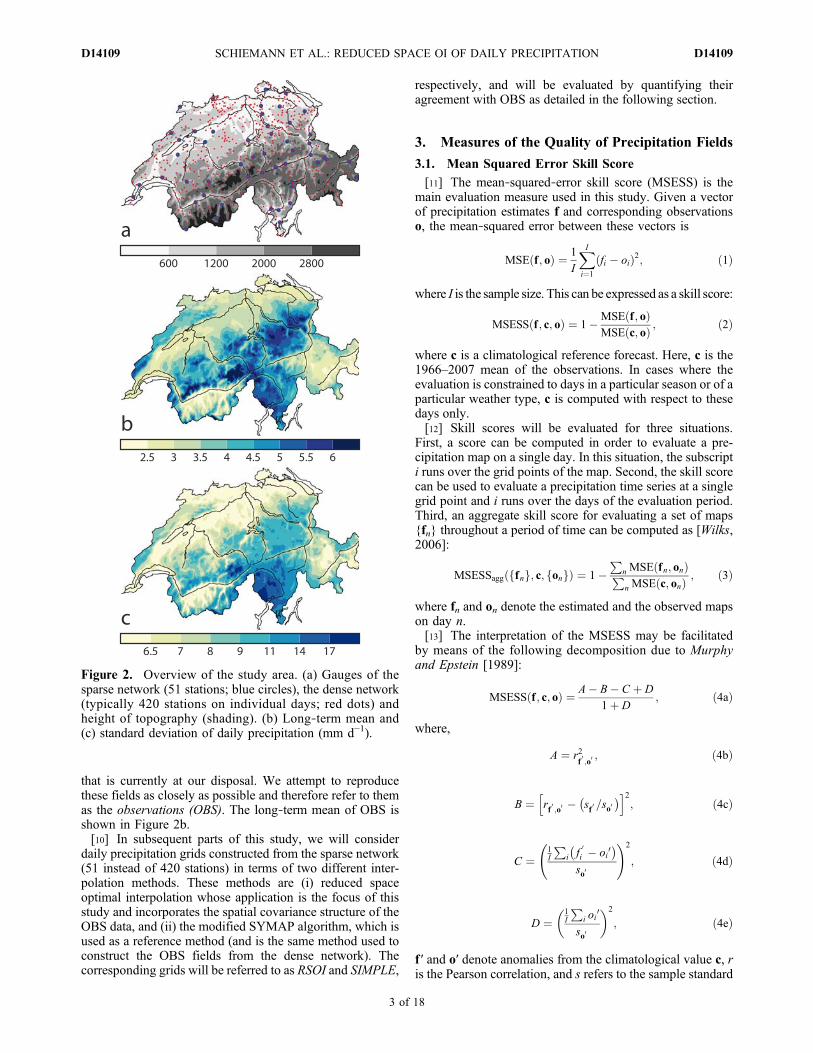
that is currently at our disposal. We attempt to reproducethese fields as closely as possible and therefore refer to themas the observations (OBS). The long‐term mean of OBS isshown in Figure 2b.[10] In subsequent parts of this study, we will consider

daily precipitation grids constructed from the sparse network(51 instead of 420 stations) in terms of two different inter-polation methods. These methods are (i) reduced spaceoptimal interpolation whose application is the focus of thisstudy and incorporates the spatial covariance structure of theOBS data, and (ii) the modified SYMAP algorithm, which isused as a reference method (and is the same method used toconstruct the OBS fields from the dense network). Thecorresponding grids will be referred to as RSOI and SIMPLE,

respectively, and will be evaluated by quantifying theiragreement with OBS as detailed in the following section.

3. Measures of the Quality of Precipitation Fields

3.1. Mean Squared Error Skill Score

[11] The mean‐squared‐error skill score (MSESS) is themain evaluation measure used in this study. Given a vectorof precipitation estimates f and corresponding observationso, the mean‐squared error between these vectors is

MSE f ; oð Þ ¼ 1

I

XIi¼1

fi � oið Þ2; ð1Þ

where I is the sample size. This can be expressed as a skill score:

MSESS f ; c; oð Þ ¼ 1�MSE f ; oð ÞMSE c; oð Þ ; ð2Þ

where c is a climatological reference forecast. Here, c is the1966–2007 mean of the observations. In cases where theevaluation is constrained to days in a particular season or of aparticular weather type, c is computed with respect to thesedays only.[12] Skill scores will be evaluated for three situations.

First, a score can be computed in order to evaluate a pre-cipitation map on a single day. In this situation, the subscripti runs over the grid points of the map. Second, the skill scorecan be used to evaluate a precipitation time series at a singlegrid point and i runs over the days of the evaluation period.Third, an aggregate skill score for evaluating a set of maps{fn} throughout a period of time can be computed as [Wilks,2006]:

MSESSagg ffng; c; fongð Þ ¼ 1�P

n MSE fn; onð ÞPn MSE c; onð Þ ; ð3Þ

where fn and on denote the estimated and the observed mapson day n.[13] The interpretation of the MSESS may be facilitated

by means of the following decomposition due to Murphyand Epstein [1989]:

MSESS f ; c; oð Þ ¼ A� B� C þ D

1þ D; ð4aÞ

where,

A ¼ r2f0;o0; ð4bÞ

B ¼ rf 0 ;o0 � sf 0 =so0� �h i2

; ð4cÞ

C ¼1I

Pi f

0i � oi0

� �so0

!2

; ð4dÞ

D ¼1I

Pi oi

0

so0

� �2

; ð4eÞ

f ′ and o′ denote anomalies from the climatological value c, ris the Pearson correlation, and s refers to the sample standard

Figure 2. Overview of the study area. (a) Gauges of thesparse network (51 stations; blue circles), the dense network(typically 420 stations on individual days; red dots) andheight of topography (shading). (b) Long‐term mean and(c) standard deviation of daily precipitation (mm d−1).

SCHIEMANN ET AL.: REDUCED SPACE OI OF DAILY PRECIPITATION D14109D14109

3 of 18

deviation. Thus, term A is simply the squared anomalycorrelation between the estimated and forecast precipitation.Terms B and C are penalties due to the conditional andunconditional (i.e. overall) biases (for details, see Murphyand Epstein [1989]).[14] A difference from the situation described by Murphy

and Epstein [1989] that is worthy of mention regards theterm D. In their study, the MSESS is used for the evaluationof large‐scale fields of geopotential height and positive andnegative values of o′ compensate such that the net contri-bution of D to the skill score is small. In the same way, theterm D will be small when evaluating time series of pre-cipitation at a single grid point in this study. It will, how-ever, not be negligible when evaluating a precipitation gridon a single day. In this case, D represents a positive con-tribution to the skill score that is independent of the estimatef. It will be the larger the more the precipitation on the dayunder consideration differs from the climatological mean c.In other words, the mean c is much worse a reference esti-mate on days that are very dry, wet, or otherwise differentfrom the climatological mean. This fact will be expressed ina higher skill score on such days. It follows immediatelyfrom this discussion that the MSESS can be applied in astraightforward way to assess two different estimates f and gof precipitation maps obtained by means of two differentmethods for the same day. Differences in the skill scoreobtained for different days, however, are partly due to thedifferences in the true precipitation distributions for thesedays and consequently much harder to interpret.

3.2. Kendall’s t Correlation

[15] As will be detailed in section 4, reduced space opti-mal interpolation aims at minimizing the interpolation errorvariance. Even though we work with transformed precipi-tation data, it might thus be argued that the MSESS is ameasure of interpolation quality that unduly favors RSOIresults. Therefore, it is interesting to test if other measures ofinterpolation quality agree with results obtained by means ofthe MSESS. We use the rank‐based t correlation of Kendall[1938] as such a complementary quality measure in a part ofthe evaluations. Recently, Mason and Weigel [2009] putforward a generic verification concept based on the two‐alternative forced choice (2AFC) test, which is applicable ina wide range of verification contexts. They have shown thatin a context where both the observations and forecasts arecontinuous variables, there is a simple relationship betweenthe p2AFC score and Kendall’s t correlation: 2 p2AFC = t + 1.[16] The use of both the MSESS and Kendall’s t corre-

lation ensures that the results presented subsequently are notan artifact of the skill measure used for evaluation. Weabstain from using object‐oriented evaluation schemes suchas SAL [Wernli et al., 2008] because the study area is smallcompared to the typical size of contiguous rainfall areas(objects) and this would introduce interpretation difficulties.

4. Reduced Space Optimal Interpolation

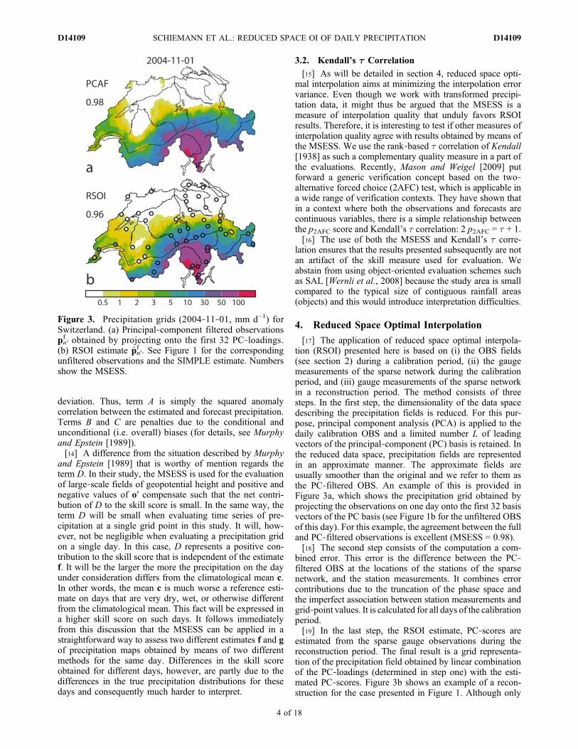
[17] The application of reduced space optimal interpola-tion (RSOI) presented here is based on (i) the OBS fields(see section 2) during a calibration period, (ii) the gaugemeasurements of the sparse network during the calibrationperiod, and (iii) gauge measurements of the sparse networkin a reconstruction period. The method consists of threesteps. In the first step, the dimensionality of the data spacedescribing the precipitation fields is reduced. For this pur-pose, principal component analysis (PCA) is applied to thedaily calibration OBS and a limited number L of leadingvectors of the principal‐component (PC) basis is retained. Inthe reduced data space, precipitation fields are representedin an approximate manner. The approximate fields areusually smoother than the original and we refer to them asthe PC‐filtered OBS. An example of this is provided inFigure 3a, which shows the precipitation grid obtained byprojecting the observations on one day onto the first 32 basisvectors of the PC basis (see Figure 1b for the unfiltered OBSof this day). For this example, the agreement between the fulland PC‐filtered observations is excellent (MSESS = 0.98).[18] The second step consists of the computation a com-

bined error. This error is the difference between the PC‐filtered OBS at the locations of the stations of the sparsenetwork, and the station measurements. It combines errorcontributions due to the truncation of the phase space andthe imperfect association between station measurements andgrid‐point values. It is calculated for all days of the calibrationperiod.[19] In the last step, the RSOI estimate, PC‐scores are

estimated from the sparse gauge observations during thereconstruction period. The final result is a grid representa-tion of the precipitation field obtained by linear combinationof the PC‐loadings (determined in step one) with the esti-mated PC‐scores. Figure 3b shows an example of a recon-struction for the case presented in Figure 1. Although only

Figure 3. Precipitation grids (2004‐11‐01, mm d−1) forSwitzerland. (a) Principal‐component filtered observationspn′f obtained by projecting onto the first 32 PC‐loadings.

(b) RSOI estimate pn′f . See Figure 1 for the corresponding

unfiltered observations and the SIMPLE estimate. Numbersshow the MSESS.

SCHIEMANN ET AL.: REDUCED SPACE OI OF DAILY PRECIPITATION D14109D14109

4 of 18

51 station values of the day have been used, the recon-struction closely resembles the analysis from the densegauge network (Figure 1b) and looks more realistic than theSIMPLE spatial analysis from the coarse network alone(Figure 1a).[20] RSOI was originally proposed byKaplan et al. [1997].

Our application closely follows the procedure described bySchmidli et al. [2001] who applied this technique for thereconstruction of monthly precipitation in the Alps. Thefollowing subsections provide a more formal description ofthe three steps of the method.

4.1. Principal Component Representation and DataSpace Reduction

[21] Let pn be the column vector of M grid point values ofthe observations on day n = 1,…, N of the calibration period(see also Table 1, and see section 5 for a discussion of thechoice of N). In order to reduce the skewness of the dailyprecipitation values, we choose to work with squared‐root‐transformed data. After removing the mean, we areleft with transformed and centered observations xn =

ffiffiffiffiffipn

p −N−1P

nffiffiffiffiffipn

p.

[22] Principal component analysis is carried out by diag-onalizing the covariance matrix Sx = (N − 1)−1

Pn xnxn

T andallows to express xn in terms of the truncated principal‐component basis:

xnM�1ð Þ

¼ EanM�Lð Þ L�1ð Þ

þ �����tnM�1ð Þ

¼: xfnM�1ð Þ

þ �����tnM�1ð Þ

; ð5Þ

where E is the matrix whose L columns are the retainedprincipal‐component loadings or EOFs (i.e. eigenvectors ofSx), an is the vector of the first L principal‐component

scores, �����nt is the error due to the dimension reduction of the

data space, and xnf are the PC‐filtered OBS on day n as, for

example, in Figure 3a. The undersets denote matrix dimen-sions. For the data at hand, the approximation is normallyrather good for phase‐space truncations with L � M suchthat, by virtue of equation (5), the problem of estimating Mgrid point values is effectively reduced to the estimation ofL scores. The choice of suitable values of L will be dis-cussed in section 5.

4.2. Computation of the Combined CalibrationPeriod Error

[23] We denote the K transformed and centered gaugemeasurements of the sparse network on day n by xn°. In orderto be able to compute a difference between the grid xn andthe gauge data xn°, each gauge of the sparse network has tobe associated with a selected cell of the observation grid.Formally, this can be written as:

x�nK�1ð Þ

¼ H�xnK�Mð Þ M�1ð Þ

þ ������nK�1ð Þ

; ð6Þ

where the matrix element Hi,j° equals one whenever gauge iis associated with grid point j and zero otherwise. Theselection is carried out as follows: For any gauge of thesparse network, we first determine the four grid cells closestto the gauge. Among these, we choose the one whose pre-cipitation time series has the highest Pearson correlationwith the gauge time series. Clearly, this association will notbe perfect since the gauge measurements are not identicalwith the grid cell values of the spatial analysis from thehigh‐resolution data set. We refer to the difference as thelocal error or association error �����n°.[24] Inserting equation (5) into (6) yields

x�nK�1ð Þ

¼ HanK�Lð Þ L�1ð Þ

þ �����rnK�1ð Þ

; where

H ¼ H�E and �����rn ¼ H������tn þ ������n:ð7Þ

Since xn°, H, and an are known during the calibration period,equation (7) allows to compute �����n

r . This is the combinederror due to both the truncation of the principal componentbasis and the imperfect association of gauges with grid cells.Its covariance matrix is estimated byR = (N− 1)−1

Pn�����n

r (�����nr )T

and is required to calculate the RSOI estimate in step three.

4.3. RSOI Estimate

[25] RSOI estimates principal‐component scores an′ forthe reconstruction period n′ = 1, …, N′ such that the fol-lowing cost function is minimized:

S an0� � ¼ �����rn0

� �TR�1�����rn01�Kð Þ K�Kð Þ K�1ð Þ

þ aTn0C�1an0

1�Lð Þ L�Lð Þ L�1ð Þ: ð8Þ

The first term in (8) is the magnitude of the combined errormeasured in terms of the statistical (Mahalanobis) metric.This ensures that error contributions from gauges that arehighly correlated will be appropriately downweighted andguarantees a fair balance of the error between regions withvariable station density. The matrix C in the second term of(8) is diagonal and its elements are the first L eigenvalues ofthe covariance matrix Sx. The role of this term is to disfavorhigh scores for higher‐order principal‐component loadings,

Table 1. Overview of Count Variables and Notation

Symbol Description

Values in ThisStudy/MatrixDimension

n = 1, …, N days in calibration period O(102–103),see sections 5, 7, 8

n′ = 1, …, N′ days in reconstruction period O(103),see sections 5, 7, 8

M grid points in OBS 13216L reduced space dimension ≤40, see section 5K gauges in the sparse network 51pn grid point precipitation on day n M × 1xn grid point precipitation (transformed) M × 1xnf PC filtered xn M × 1xn′f OI estimate of xn′

f M × 1xn° gauge values (transformed) K × 1Sx covariance of xn M × ME PC loadings (EOFs) M × LH° gauge‐grid point association K × MH H°E K × Lan PC scores L × 1an′ OI estimate of an′ L × 1�����nt truncation error M × 1�����n° association error K × 1�����nr combined error K × 1R combined error covariance K × KC leading eigenvalues of Sx (diagonal) L × LP OI estimation error covariance L × LP~

OI reconstruction error covariance M × MCr covariance of �����n

t M × MP total reconstr. error covariance M × MP(+) upper bound on P M × M

SCHIEMANN ET AL.: REDUCED SPACE OI OF DAILY PRECIPITATION D14109D14109

5 of 18

i.e. patterns that had “historically little energy” [Kaplan et al.,1997].[26] There is an analytical solution for an′ that minimizes

the cost function. It reads

an0L�1ð Þ

¼ PHTR�1x�n0

L�Lð Þ L�Kð Þ K�Kð Þ K�1ð Þ;

P ¼ HTR�1Hþ C�1� ��1;

ð9Þ

where P is the covariance matrix of the OI estimation errorin the reduced space.[27] Finally, a grid representation of the reconstruction in

transformed and centered coordinates is recovered by

xfn0

M�1ð Þ¼ E an0

M�Lð Þ L�1ð Þ; ð10Þ

where xn′f is the OI estimate of the PC‐filtered observations

xn′f . Subsequent backtransformation yields the reconstruction

in precipitation units. In the backtransformation, unphysicalnegative estimates are set to zero before squaring.[28] An estimate of the reconstruction error variance can

be obtained via

~P

M�Mð Þ¼ EPET

M�Lð Þ L�Lð Þ L�Mð Þ; ð11Þ

the covariance matrix of the estimation error xn′f − xn′

f . It canbe shown that the covariance matrix P of the total recon-struction error xn′

f −xn′ including the truncation error (com-pare (5)) satisfies

P � 2 ~Pþ Cr� �

¼: P þð Þ; ð12Þ

where Cr is the covariance matrix of the truncation error �����nt ,

and P is the covariance matrix of the total reconstructionerror (symmetric real matrices A and B are said to be inrelation A ≤ B if xT (B− A)x ≥ 0 ∀ x).

5. Sampling Variability and Sensitivityto the Reduced Space Dimension

[29] In this section, we examine the sensitivity of theinterpolation results to the choice of the reduced spacedimension L and to the number of days N used for cali-brating the statistical model. This will help to find appro-priate choices of these parameters. The sensitivity studyencompasses two steps. In a first step (section 5.1), wedetermine how the aggregate skill over an extended recon-struction period depends on the choice of L and N. In asecond step (section 5.2), we examine the robustness of thereconstruction on individual days to the choice of L and N.Note that even if the aggregate score is very similar for twochoices of L and N, the reconstructed fields might differconsiderably on individual days. Ideally, such differencesare small such that for any single day the interpolated fieldsare “reproducible” in the sense that they do not stronglydepend on the choice of the calibration parameters butexclusively on the sparse gauge data in the reconstructionperiod. Both the aggregate and daily analyses will be carriedout separately for the truncation error and the total recon-struction error.

5.1. Aggregate Reconstruction Skill

[30] We conduct the following experiment: For each ofa number of sample sizes Ni = 100,500,2000, six sets ofdays are chosen randomly from the set of all days in 1971–1990. We denote the corresponding subsets of OBS by{xn}i,k with k = 1, …, 6. For each of these calibration sets,principal component analysis is carried out and the principal‐component basis is truncated for a range of subspacedimensions Lj. Thereafter, independent observations (for alldays n′ in 1995–1998) are projected onto the reduced dataspaces. This yields filtered observations {xn′

f }i, j,k that areevaluated by means of the aggregated skill score defined in(3). In this exercise, PCA is carried out in terms of thetransformed data, but for the calculation of the skill scoresthe untransformed data are used.[31] Figure 4 depicts the resulting aggregate skill scores

for different L, N, and for each of the replicates. For areduced space of only L = 40 dimensions the truncation erroris very small and the skill score of the filtered observationsis as high as MSESS = 0.96 (note that the dimensionality ofthe full data space is equal to the number of grid points M =13216). Moreover, it shows that sampling variability is not aserious issue even for short calibration periods. Sizeabledifferences between the calibration samples are only foundfor N = 100 and very low L. This is due to the fact that theskill of principal‐component filtering depends on the entiresubspace that is spanned by the truncated basis. This sub-space appears to be much more robust than estimates ofindividual basis vectors.[32] The sensitivity experiment is continued by computing

the RSOI estimates {xn′f }i, j,k (again throughout the 4‐yearevaluation period 1995–1998) following equations (9) and(10). Figure 5 is analogous to Figure 4 and shows the skillscores associated with the total reconstruction error, i.e.MSESSagg({pn′

f }i, j,k, c, {pn′}i,k). Here, the sampling vari-ability is somewhat larger than for principal‐componentfiltering only, but it is still very small if N^ 500 and L^ 12.The reconstruction skill score saturates at a value ofMSESS ≈0.89 for L^ 24, while the corresponding principal‐component‐filtering skill continues to increase with L as shown by thedotted lines. Obviously, the reconstruction skill for N ^ 500and L ^ 12 is limited by the sparse gauge observationsrather than by the truncation of the data space or the limitedcalibration period.

5.2. Robustness of RSOI Results on Single Days

[33] The results presented in the following are obtainedfrom the experiment described in section 5.1, but here, theanalysis focuses on the robustness of the PC filtering and theRSOI reconstruction for individual days. That is, skill scoresare calculated individually for each day and for each of the sixreplicates according to equation (2). A measure of robustnesscan be obtained by calculating the standard deviation of thesix skill scores for each day. This yields a daily times series ofthe skill spread for each setting of N and L.[34] Figure 6 shows box‐plot statistics of these time series

for some combinations of N and L. The closer these dis-tributions are to the zero line, the more similar (or, strictlyspeaking, similar in quality as measured by the MSESS) aredifferent realizations of daily PC‐filtered OBS. Figure 6shows that this similarity (or robustness) increases with L,

SCHIEMANN ET AL.: REDUCED SPACE OI OF DAILY PRECIPITATION D14109D14109

6 of 18

if the number of calibration days N is small. This is con-sistent with the above discussion: Even though the estima-tion of individual basis vectors of the reduced space must beexpected to be subject to substantial sampling variability forsmall N, the reduced space spanned by the L basis vectorsjointly is decisive for the present application and principal‐component filtering becomes more robust with increasing L.Figure 6 also shows that the robustness increases with N aslong as N ] 1000.[35] If this kind of analysis is extended to the RSOI esti-

mates (Figure 7), it can be seen that the robustness is smaller(i.e. the skill variance is larger) than for principal‐componentfiltering. Arguably, this is due to the fact that differencesbetween the realizations are not only caused by differencesin the reduced spaces, but also by how well the sparse gaugeobservations can capture scores of individual principal‐component modes on a given day. Nevertheless, for N ^1000, the standard deviation of the daily skill scores istypically on the order of 0.01 and only O(0.1) for very fewdays, whereas the skill score itself is O(1). It is in this sensethat we can affirm that the results from RSOI are robust tothe reduced space dimension and to the observations usedfor calibration.[36] The above analyses are used to choose values of N

and L for an RSOI that will be evaluated in subsequent parts

of the paper. It has been shown that the interpolation skilldoes not increase meaningfully for N ^ 500. However, therobustness of the interpolation results for individual daysdoes increase if N is further increased and it is reasonableto do this if it can be afforded. Here, we choose N = 2000.The value of L is of little importance as long as it isgreater than about 20. Arguably, this is due to the fact thatoverfitting for large values of L is impeded by the penaltyfor higher‐order PCs in the second term of (8). The choicemade here is L = 32.

6. PCA Results

[37] Principal component analysis is the first step of eachRSOI reconstruction and the results obtained are reportedbriefly in this section. The analysis is carried out asdescribed in section 4.1 and is based on the OBS fields ofN = 2000 randomly chosen days in 1971–1980. The firstfour eigenvectors are shown in Figure 8. The first is a uni-form pattern and simply discerns dry and wet situations inthe whole study domain. It explains 67% of the total vari-ability. The second and third PCs are bipolar. The secondrepresents a north–south gradient of precipitation thatapproximately follows the main Alpine ridge, whereas thethird contrasts the west and east of Switzerland. The fourth

Figure 4. Evaluation of the principal‐component‐filtered precipitation grids as a function of the numberN of observations (days) used for PCA and the number of retained principal components L. For each N,six independent sets of observations have been drawn. The bars show the aggregated MSESS for eachrealization, each L, and each N. The numbers show the mean of these values across the six realizations.The horizontal dashed line shows this mean for N = 2000 and L = 40.

SCHIEMANN ET AL.: REDUCED SPACE OI OF DAILY PRECIPITATION D14109D14109

7 of 18

Figure 5. Same as Figure 4 but for RSOI results. The horizontal dotted lines correspond to the skill scorefor principal‐component filtering shown in Figure 4. The horizontal dashed line shows the aggregateMSESS (mean over 6 realizations) for the reconstruction with N = 2000 and L = 40.

Figure 6. Robustness of principal‐component‐filtered grids on individual days. On each day, theMSESS has been computed for six realizations for each combination of N and L. The daily spread ofMSESS (the standard deviation obtained from the MSESS of the six realizations) has been computedand its distribution over time is shown by means of box‐and‐whiskers plots.

SCHIEMANN ET AL.: REDUCED SPACE OI OF DAILY PRECIPITATION D14109D14109

8 of 18

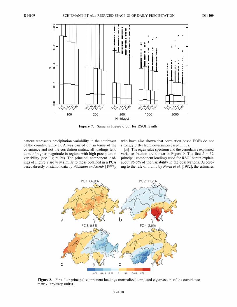
pattern represents precipitation variability in the southwestof the country. Since PCA was carried out in terms of thecovariance and not the correlation matrix, all loadings tendto be of higher magnitude in regions with high precipitationvariability (see Figure 2c). The principal‐component load-ings of Figure 8 are very similar to those obtained in a PCAbased directly on station data byWidmann and Schär [1997],

who have also shown that correlation‐based EOFs do notstrongly differ from covariance‐based EOFs.[38] The eigenvalue spectrum and the cumulative explained

variance fraction are shown in Figure 9. The first L = 32principal‐component loadings used for RSOI herein explainabout 96.6% of the variability in the observations. Accord-ing to the rule of thumb by North et al. [1982], the estimates

Figure 7. Same as Figure 6 but for RSOI results.

Figure 8. First four principal‐component loadings (normalized unrotated eigenvectors of the covariancematrix; arbitrary units).

SCHIEMANN ET AL.: REDUCED SPACE OI OF DAILY PRECIPITATION D14109D14109

9 of 18

of the first 12 EOFs can be expected to be individuallyrobust.

7. Evaluation of RSOI Reconstructions

[39] This section is concerned with the systematic evalu-ation of RSOI results. The PCA step of RSOI is as in section6 (L = 32, N = 2000). The reconstruction period consists ofall days in 2001–2007, i.e. it is independent of the calibra-tion period. The following subsections present examples ofreconstructed fields, compare the RSOI reconstruction to theSIMPLE reference interpolation, and discuss the propertiesof the reconstruction errors.

7.1. Examples

[40] Here, some examples of interpolated precipitationgrids are presented for situations where RSOI performs eitherexceptionally well or badly. As discussed in section 3.1, theMSESS is not a suitable measure for comparing the recon-struction skill between different days. For selecting a fewillustrative cases in this section, we have used a pragmaticmodification of MSESS, namely the quantity A ‐ B ‐ C inequation (4a) as a guideline. This measure is dominated bythe pattern correlation (equation (4b)). We have ranked alldays in the reconstruction period according to this quantityand present results for days with the highest and lowestranks in Figures 10 and 11, respectively.[41] Figure 10 shows that very good RSOI results are

obtained when the precipitation pattern resembles one of theleading PC loadings (see Figure 8). For example, the second

loading can be clearly discerned on 2002‐11‐15, 2004‐10‐28(Figures 10f and 10o), and the third EOF on 2004‐03‐13 and2002‐04‐24 (Figures 10c and 10i). In such situations, themaps obtained by RSOI agree very well with the OBS fieldsand correctly represent mesoscale patterns of the precipita-tion distribution that are not captured by the sparse networkalone. For example, the location of the boundary betweenregions with and without precipitation occurrence on 2002‐10‐15 is well represented in Figure 10k, even though muchof this boundary is quite distant from gauges of the sparsenetwork. As a further example, consider the RSOI estimatesin the Engadin region (the valley of the Inn, the easternmostriver on the maps, and surroundings) on 2002‐11‐15 and2002‐04‐24 (Figures 10e and 10h). It is not surprising thatfor these cases the SIMPLE interpolation from the sparsenetwork alone is inferior to RSOI. This is supported by thevalues of theMSESS aswell as by the inspection of the contourplots: The SIMPLE fields depend markedly on the locationof the gauges and exhibit unreasonably strong gradients andkinks. As an example, consider again the representation ofthe precipitation gradient on 2002‐10‐15 (Figure 10j).[42] As a complement, Figure 11 depicts a number of cases

with particularly poor performance of RSOI. The observa-tions in Figures 11c, 11f, 11i, 11l, and 11o show that the poorperformance is associated with precipitation distributionswhich are hardly captured by the sparse network or whichdiffer markedly from the leading PC loadings or combina-tions thereof. All cases considered in Figure 11 fall into thewarm season and appear to be associated with summerconvection as is evident in the scattered distributions. The

Figure 9. Scree plot: explained variance (gray bars and logarithmic axis on the right) and cumulativeexplained variance fraction (blue line and left axis). Narrow black boxes show an estimate of the samplingerror in the Lth eigenvalue based on the rule of thumb by North et al. [1982].

SCHIEMANN ET AL.: REDUCED SPACE OI OF DAILY PRECIPITATION D14109D14109

10 of 18

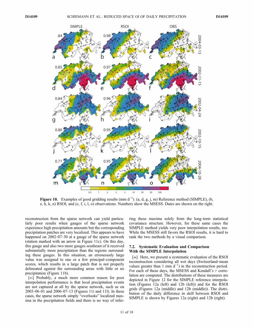
reconstruction from the sparse network can yield particu-larly poor results when gauges of the sparse networkexperience high precipitation amounts but the correspondingprecipitation patches are very localized. This appears to havehappened on 2002‐07‐30 at a gauge of the sparse network(station marked with an arrow in Figure 11c). On this day,this gauge and also two more gauges southeast of it receivedsubstantially more precipitation than the regions surround-ing these gauges. In this situation, an erroneously largevalue was assigned to one or a few principal‐componentscores, which results in a large patch that is not properlydelineated against the surrounding areas with little or noprecipitation (Figure 11b).[43] Probably, a much more common reason for poor

interpolation performance is that local precipitation eventsare not captured at all by the sparse network, such as on2003‐06‐01 and 2006‐07‐13 (Figures 11i and 11l). In thesecases, the sparse network simply “overlooks” localized max-ima in the precipitation fields and there is no way of infer-

ring these maxima solely from the long‐term statisticalcovariance structure. However, for these same cases theSIMPLE method yields very poor interpolation results, too.While the MSESS still favors the RSOI results, it is hard torank the two methods by a visual comparison.

7.2. Systematic Evaluation and ComparisonWith the SIMPLE Interpolation

[44] Here, we present a systematic evaluation of the RSOIreconstruction considering all wet days (Switzerland‐meanvalues greater than 1 mm d−1) in the reconstruction period.For each of these days, the MSESS and Kendall’s t corre-lation are computed. The distributions of these measures aredepicted in Figure 12 for the SIMPLE reference interpola-tion (Figures 12a (left) and 12b (left)) and for the RSOIgrids (Figures 12a (middle) and 12b (middle)). The distri-bution of the daily difference in skill between RSOI andSIMPLE is shown by Figures 12a (right) and 12b (right).

Figure 10. Examples of good gridding results (mm d−1). (a, d, g, j, m) Reference method (SIMPLE), (b,e, h, k, n) RSOI, and (c, f, i, l, o) observations. Numbers show the MSESS. Dates are shown on the right.

SCHIEMANN ET AL.: REDUCED SPACE OI OF DAILY PRECIPITATION D14109D14109

11 of 18

[45] Clearly, the RSOI grids tend to have a higher MSESSthan the SIMPLE grids (Figure 12a). The aggregate skillscore for the SIMPLE method is ≈0.77 whereas the samenumber for RSOI is ≈0.87. This difference in quality can befound throughout the distribution of the skill score. Whilethere is, for example, only a handful of days when RSOI hasa negative skill, there is a good few more in the case ofSIMPLE as shown by the long lower tail of the skill scoredistribution. Also, the differences in the score between bothmethods on each day reveal that there is an added value inthe RSOI fields over the SIMPLE reference fields except forvery few days (61 out of 1234). The results from an anal-ogous evaluation in terms of Kendall’s t correlation cor-roborate the above (Figure 12b): The entire distribution ofthe daily values of t is shifted to higher values for the RSOIresults and, according to this skill measure, there are only142 days when the SIMPLE interpolations are of higherquality than the RSOI maps.[46] The evaluation in Figure 12b suggests a seasonal

dependence of the interpolation skill. For both interpolation

methods, better results are obtained during the cold season.This is in line with the discussion in section 7.1, wheredifficulties were primarily found for localized precipitationpatterns typical for summer convection. The differences in tbetween the seasons are more pronounced for the RSOI thanfor the SIMPLE method. That is, the improvement due tothe application of RSOI is somewhat smaller during sum-mer. Arguably, this is partly due to the fact that the leadingprincipal components explain a smaller fraction of the totalvariance in summer and that the smaller‐scale variability ofsummer rainfall exerts larger sampling errors in the esti-mation of the PC scores from the coarse network.[47] We conclude this discussion by considering the

spatial variation of the interpolation skill. CorrespondingMSESS maps are shown in Figure 13. It can be seen that theskill of the SIMPLE interpolation is higher than that ofRSOI in very close proximity to the gauges of the sparsenetwork. With increasing distance from the gauge locations,however, the SIMPLE skill decreases rapidly and is clearlylower than the RSOI skill in most of the domain. For both

Figure 11. Same as Figure 10 but for cases where gridding from the sparse network is very difficult.

SCHIEMANN ET AL.: REDUCED SPACE OI OF DAILY PRECIPITATION D14109D14109

12 of 18

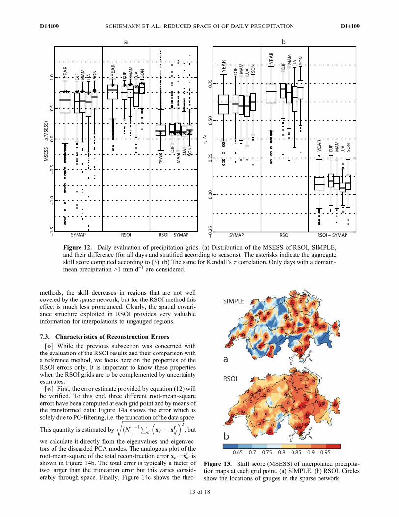
methods, the skill decreases in regions that are not wellcovered by the sparse network, but for the RSOI method thiseffect is much less pronounced. Clearly, the spatial covari-ance structure exploited in RSOI provides very valuableinformation for interpolations to ungauged regions.

7.3. Characteristics of Reconstruction Errors

[48] While the previous subsection was concerned withthe evaluation of the RSOI results and their comparison witha reference method, we focus here on the properties of theRSOI errors only. It is important to know these propertieswhen the RSOI grids are to be complemented by uncertaintyestimates.[49] First, the error estimate provided by equation (12) will

be verified. To this end, three different root‐mean‐squareerrors have been computed at each grid point and bymeans ofthe transformed data: Figure 14a shows the error which issolely due to PC‐filtering, i.e. the truncation of the data space.

This quantity is estimated by

ffiffiffiffiffiffiffiffiffiffiffiffiffiffiffiffiffiffiffiffiffiffiffiffiffiffiffiffiffiffiffiffiffiffiffiffiffiffiffiffiffiffiffiffiffiffiN 0ð Þ�1P

n0 xn0 � xfn0

� �2r, but

we calculate it directly from the eigenvalues and eigenvec-tors of the discarded PCA modes. The analogous plot of theroot‐mean‐square of the total reconstruction error xn′ −xn′f isshown in Figure 14b. The total error is typically a factor oftwo larger than the truncation error but this varies consid-erably through space. Finally, Figure 14c shows the theo-

Figure 12. Daily evaluation of precipitation grids. (a) Distribution of the MSESS of RSOI, SIMPLE,and their difference (for all days and stratified according to seasons). The asterisks indicate the aggregateskill score computed according to (3). (b) The same for Kendall’s t correlation. Only days with a domain‐mean precipitation >1 mm d−1 are considered.

Figure 13. Skill score (MSESS) of interpolated precipita-tion maps at each grid point. (a) SIMPLE. (b) RSOI. Circlesshow the locations of gauges in the sparse network.

SCHIEMANN ET AL.: REDUCED SPACE OI OF DAILY PRECIPITATION D14109D14109

13 of 18

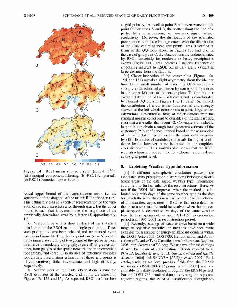
retical upper bound of the reconstruction error, i.e. thesquare root of the diagonal of the matrix P(+) defined in (12).This estimate yields an excellent representation of the vari-ation of the reconstruction error through space, but the upperbound is such that it overestimates the magnitude of theempirically determined error by a factor of, approximately,1.5.[50] We continue with a short analysis of the statistical

distribution of the RSOI errors at single grid points. Threesuch grid points have been selected and are marked by anasterisk in Figure 14. The selected points are (case A) locatedin the immediate vicinity of two gauges of the sparse networkin an area of moderate topography, (case B) at greater dis-tance from gauges of the sparse network and in intermediatetopography, and (case C) in an area of extremely complextopography. Precipitation estimation at these grid points isof comparatively little, intermediate, and high difficulty,respectively.[51] Scatter plots of the daily observations versus the

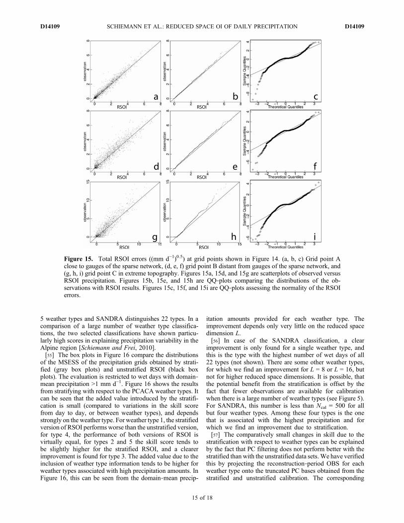
RSOI estimates at the selected grid points are shown inFigures 15a, 15d, and 15g. As expected, RSOI performs best

at grid point A, less well at point B and even worse at gridpoint C. For cases A and B, the scatter about the line of aperfect fit is rather uniform, i.e. there is no sign of hetero-scedasticity. Moreover, the distribution of the estimatedprecipitation is in excellent agreement with the distributionof the OBS values at these grid points. This is verified interms of the QQ‐plots shown in Figures 15b and 15e. Inthe case of grid point C, the observations are underestimatedby RSOI, especially for moderate to heavy precipitationevents (Figure 15h). This indicates a general tendency ofsmoothing inherent to RSOI, but is only really evident atlarge distance from the stations.[52] Closer inspection of the scatter plots (Figures 15a,

15d, and 15g) reveals a slight asymmetry about the identityline. On a small number of days, the OBS values arestrongly underestimated as shown by corresponding entriesin the upper‐left part of the scatter plots. This points to askewed distribution of the RSOI errors and is corroboratedby Normal‐QQ‐plots in Figures 15c, 15f, and 15i. Indeed,the distribution of errors is far from normal and stronglyskewed to the left which corresponds to some large under-estimations. Nevertheless, most of the deviations from thestandard normal correspond to quantiles of the standardizederror that are smaller than about −2. Consequently, it shouldbe possible to obtain a rough (and generous) estimate of thecustomary 95% confidence interval based on the assumptionof normally distributed errors and the error variance givenby (12). Estimates of confidence intervals for higher confi-dence levels, however, must be based on the empiricalerror distribution. This analysis also shows that the RSOIreconstructions are not suitable for extreme value analysesat the grid‐point level.

8. Exploiting Weather Type Information

[53] If different atmospheric circulation patterns areassociated with precipitation distributions belonging to dif-ferent areas of the data space, weather type informationcould help to further enhance the reconstructions. Here, wetest if the RSOI skill improves when the method is cali-brated only with days of the same weather type as the dayfor which the reconstruction is carried out. One expectationof this stratified application of RSOI is that more detail onthe covariance structure could be resolved when the reducedphase‐space is determined by days of the same weathertype. In this experiment, we use 1971–1995 as calibrationperiod and 1996–2002 as reconstruction period.[54] Recently, catalogs of weather types based on a wide

range of objective classification methods have been madeavailable for a number of European standard domains withinthe COST Action 733 (COST733, Harmonisation and Appli-cations ofWeather Type Classifications for EuropeanRegions,2005, http://www.cost733.org). We use two of these catalogsderived by means of classification methods referred to asPCACA [Rasilla Álvarez, 2003; García Codron and RasillaÁlvarez, 2006] and SANDRA [Philipp et al., 2007]. Bothcatalogs rely on sea‐level‐pressure fields from the ERA40re‐analysis (1958–2002) [Uppala et al., 2005] and areavailable with daily resolution throughout the ERA40 period.For the COST 733 standard domain covering the Alps andadjacent regions, the PCACA classification distinguishes

Figure 14. Root‐mean square errors ((mm d−1)0.5).(a) Principal‐component filtering. (b) RSOI (empirical).(c) RSOI (theoretical upper bound).

SCHIEMANN ET AL.: REDUCED SPACE OI OF DAILY PRECIPITATION D14109D14109

14 of 18

5 weather types and SANDRA distinguishes 22 types. In acomparison of a large number of weather type classifica-tions, the two selected classifications have shown particu-larly high scores in explaining precipitation variability in theAlpine region [Schiemann and Frei, 2010].[55] The box plots in Figure 16 compare the distributions

of the MSESS of the precipitation grids obtained by strati-fied (gray box plots) and unstratified RSOI (black boxplots). The evaluation is restricted to wet days with domain‐mean precipitation >1 mm d−1. Figure 16 shows the resultsfrom stratifying with respect to the PCACA weather types. Itcan be seen that the added value introduced by the stratifi-cation is small (compared to variations in the skill scorefrom day to day, or between weather types), and dependsstrongly on the weather type. For weather type 1, the stratifiedversion of RSOI performs worse than the unstratified version,for type 4, the performance of both versions of RSOI isvirtually equal, for types 2 and 5 the skill score tends tobe slightly higher for the stratified RSOI, and a clearerimprovement is found for type 3. The added value due to theinclusion of weather type information tends to be higher forweather types associated with high precipitation amounts. InFigure 16, this can be seen from the domain‐mean precip-

itation amounts provided for each weather type. Theimprovement depends only very little on the reduced spacedimension L.[56] In case of the SANDRA classification, a clear

improvement is only found for a single weather type, andthis is the type with the highest number of wet days of all22 types (not shown). There are some other weather types,for which we find an improvement for L = 8 or L = 16, butnot for higher reduced space dimensions. It is possible, thatthe potential benefit from the stratification is offset by thefact that fewer observations are available for calibrationwhen there is a large number of weather types (see Figure 5).For SANDRA, this number is less than Ncal = 500 for allbut four weather types. Among these four types is the onethat is associated with the highest precipitation and forwhich we find an improvement due to stratification.[57] The comparatively small changes in skill due to the

stratification with respect to weather types can be explainedby the fact that PC filtering does not perform better with thestratified than with the unstratified data sets. We have verifiedthis by projecting the reconstruction‐period OBS for eachweather type onto the truncated PC bases obtained from thestratified and unstratified calibration. The corresponding

Figure 15. Total RSOI errors ((mm d−1)0.5) at grid points shown in Figure 14. (a, b, c) Grid point Aclose to gauges of the sparse network, (d, e, f) grid point B distant from gauges of the sparse network, and(g, h, i) grid point C in extreme topography. Figures 15a, 15d, and 15g are scatterplots of observed versusRSOI precipitation. Figures 15b, 15e, and 15h are QQ‐plots comparing the distributions of the ob-servations with RSOI results. Figures 15c, 15f, and 15i are QQ‐plots assessing the normality of the RSOIerrors.

SCHIEMANN ET AL.: REDUCED SPACE OI OF DAILY PRECIPITATION D14109D14109

15 of 18

(stratified and unstratified) explained variance fractions arefound to be nearly equal, even for very small values of L(Table 2).

9. Conclusions and Discussion

[58] RSOI is a statistical procedure which allows toreconstruct daily precipitation fields from measurements ofsparse station networks. It has been shown that this methodcan be applied to root‐transformed daily precipitation datain a straightforward way. It is inherent to RSOI that ityields spatially smoothed precipitation fields. Nevertheless,gridding in terms of RSOI clearly outperforms a referenceinterpolation method (based on contemporaneous gaugedata only) for the study domain and the networks consideredherein. This holds true for all seasons. The added value issomewhat smaller for summer than for the other seasons.The improvement over the reference method is particularlystrong for locations at greater distance from the gauge loca-tions. Consequently, RSOI lends itself to gridding in a quasireal‐time context, when only measurements of a small part of

the full gauge network are available. The interpolation pre-sented herein is entirely based on gauge measurementsand their covariance in space, it does not use other sources ofdata such as radar measurements [e.g., Gjertsen et al., 2004;DeGaetano and Wilks, 2009]. Thus, RSOI is attractive as areference for methods using additional data sources, or insituations when no additional data are available.[59] It was a further objective of this study to test if

stratification with respect to weather types can increase thereconstruction skill. It has been shown that this improve-ment is comparatively small and depends strongly on theweather type. Stratification is generally more beneficial forwet weather types than for dry types. Moreover, there isindication that the reduction in sample size associated withthe stratification may offset the potential benefits fromweather type information.[60] Our analyses allow for a number of conclusions

regarding potential operational implementations. A sensi-tivity analysis has shown that neither the number of daysavailable for calibration nor the truncation of the data spaceare critical issues. It has been shown that the skill score of

Figure 16. Distribution of daily MSESS for unstratified RSOI (black) and RSOI stratified according tothe five PCACA weather types (gray). For each weather type, the annotations refer to the number of daysof the weather type in the calibration and reconstruction periods (Ncal, Nrec), the number of days Nrec

wet ofthe weather type with domain‐mean precipitation >1 mm d−1, and the domain‐mean precipitation (p, mmd−1) for the weather type considered.

Table 2. Cumulative Explained Variance Fractiona

Reduced SpaceDimension L

PCACA Weather Type

1 2 3 4 5

L = 1 0.387 (0.382) 0.512 (0.509) 0.526 (0.515) 0.448 (0.450) 0.501 (0.495)L = 8 0.800 (0.797) 0.869 (0.866) 0.896 (0.887) 0.833 (0.830) 0.895 (0.890)

aFor the projection of reconstruction‐period OBS (>1 mm d−1) of a weather type onto the PC basis derived (1) from calibration‐period OBS of the sameweather type and (2) from calibration‐period OBS of arbitrary weather type (numbers in parentheses).

SCHIEMANN ET AL.: REDUCED SPACE OI OF DAILY PRECIPITATION D14109D14109

16 of 18

the RSOI fields saturates as soon as there are about 500 daysavailable for calibration. If the number of observations forcalibration is increased beyond this number, this does notresult in a sizeable improvement of the time‐mean griddingskill, but still reduces the dependence of the day‐to‐dayRSOI estimates on the calibration sample. Furthermore,RSOI errors have been shown to not follow a Gaussian dis-tribution. In particular, the RSOI estimates strongly under-estimate the observed precipitation on some days and thisoccurs more frequently than the assumption of normallydistributed errors would suggest. Consequently, estimatesof the uncertainty of RSOI grids should be based on theempirical errors whenever possible. Stratification withrespect to weather types may increase the interpolation skillby a small amount, but this has to be tested for each weathertype. Two further practical issues should be born in mind.First, it is a convenient feature of RSOI that the computa-tionally more demanding calibration of the method has to becarried out only once if near‐real‐time reconstructions are tobe provided on a daily basis. Second, it is important to notethat the method depends on the availability of the sparsenetwork data during both the calibration and reconstructionperiods. Missing values at individual stations of the sparsenetwork during the reconstruction period, however, can behandled without repetition of the calibration step.[61] It has been shown that the RSOI results should be

interpreted with particular care when the sparse network isnot representative for the precipitation pattern and, at thesame time, the pattern is “unusual” in the sense that it cannot be expressed as a combination of a few leading EOFs ofthe precipitation climatology. These situations normallyoccur in summer and appear to be associated with highlylocalized convective events not linked directly to topo-graphic effects. However, also the reference interpolationmethod considered herein yields unsatisfactory results insuch cases.[62] Naturally, there is a number of open questions that

await further investigation. In a quantitative sense, theresults obtained in this study hold for the particular caseconsidered here. Qualitatively, they should carry over tocomparable situations. Systematic analyses regarding thedependence of the performance of RSOI on the size and thegeographic setting of the study area, and on the character-istics of the sparse and dense networks are still missing. Inparticular, the applicability of RSOI in flat terrain, whereprecipitation patterns could be less recurrent and possiblyless well approximated by means of a few leading principalcomponents, remains to be tested. Especially if the focus ison the distinction of wet and dry situations, precipitationshould be modeled as a mixed distribution treating dry casesseparately [e.g., Bell, 1987]. If an approach of this kindcould be incorporated into the RSOI framework, this wouldcertainly constitute a substantial improvement of themethod. Furthermore, it is conceivable that RSOI can alsobe used to take reconstructed historical precipitation [e.g.,New et al., 2002; Schmidli et al., 2001; Brunetti et al., 2006;Efthymiadis et al., 2006] to the daily scale, but the evalua-tion in this study did not focus on this issue. Here, it hasbeen shown that RSOI is a candidate for real‐time dailyprecipitation gridding and that it is worthwhile to carry outanalyses of the kind mentioned above in order to optimizethe method for a particular application.

[63] Acknowledgments. This study benefited from the scientificexchange in the community of COST Action 733 “Harmonisationand applications of weather type classifications for European regions”chaired by Ole Einar Tveito. Sincere thanks are given to Andreas Philippand Domingo Rasilla Álvarez for the provision of weather type data. Further-more, we would like to thank Sandy Ubl, Andreas Weigel, Joaquim CollMolinos, and Christof Appenzeller for discussion. This work was supportedby the Swiss State Secretariat for Education and Research (COST Action733, SBF C06.0077).

ReferencesAllan, R., and T. Ansell (2006), A new globally complete monthly historicalgridded mean sea level pressure dataset (HadSLP2): 1850–2004, J Clim.,19, 5816–5842.

Ansell, T. J., et al. (2006), Daily mean sea level pressure reconstructions forthe European–North Atlantic region for the period 1850–2003, J. Clim.,19, 2717–2742.

Bell, T. L. (1987), A space‐time stochastic model of rainfall for satelliteremote‐sensing studies, J. Geophys. Res., 92(D8), 9631–9643.

Brunetti, M., M. Maugeri, T. Nanni, I. Auer, R. Böhm, and W. Schöner(2006), Precipitation variability and changes in the greater Alpine regionover the 1800–2003 period, J. Geophys. Res., 111, D11107, doi:10.1029/2005JD006674.

Courault, D., and P. Monestiez (1999), Spatial interpolation of air temper-ature according to atmospheric circulations patterns in southeast France,Int. J. Climatol., 19, 365–378.

DeGaetano, A. T., and D. S. Wilks (2009), Radar‐guided interpolation ofclimatological precipitation data, Int. J. Climatol., 29, 185–196,doi:10.1002/joc.1714.

Dorninger, M., S. Schneider, and R. Steinacker (2008), On the interpolationof precipitation data over complex terrain, Meteorol. Atmos. Phys., 101,175–189, doi:10.1007/s00703-008-0287-6.

Efthymiadis, D., P. D. Jones, K. R. Briffa, I. Auer, R. Böhm, W. Schöner,C. Frei, and J. Schmidli (2006), Construction of a 10‐min‐gridded pre-cipitation data set for the Greater Alpine Region for 1800–2003, J. Geo-phys. Res., 111, D01105, doi:10.1029/2005JD006120.

Erdin, R. (2009), Combining rain gauge and radar measurements of a heavyprecipitation event over Switzerland, Master’s thesis, MeteoSwiss andETH Zurich, Zurich, Switzerland.

Evans, M. N., A. Kaplan, and M. A. Cane (2002), Pacific sea surface tem-perature field reconstruction from coral d18 data using reduced spaceobjective analysis, Paleoceanography, 17(1), 1007, doi:10.1029/2000PA000590.

Frei, C., and C. Schär (1998), A precipitation climatology of the Alps fromhigh‐resolution rain‐gauge observations, Int. J. Climatol., 18, 873–900.

Frei, C., R. Schöll, S. Fukutome, J. Schmidli, and P. L. Vidale (2006),Future change of precipitation extremes in Europe: Intercomparison ofscenarios from regional climate models, J. Geophys. Res., 111,D06105, doi:10.1029/2005JD005965.

Frei, C., U. Germann, S. Fukutome, and M. Liniger (2008), Möglichkeitenund Grenzen der Niederschlagsanalysen zum Hochwasser 2005, Tech.Rep. 221, MeteoSwiss, Zurich, Switzerland.

García Codron, J. C., and D. F. Rasilla Álvarez (2006), Coastline retreat,sea level variability and atmospheric circulation in Cantabria (NorthernSpain), J. Coastal Res., SI 48, 49–54.

Germann, U., G. Galli, M. Boscacci, and M. Bolliger (2006), Radar precip-itation measurement in a mountainous region, Q. J. R. Meteorol. Soc.,132, 1669–1692, doi:10.1256/qj.05.190.

Gjertsen, U., M. Šalek, and D. B. Michelson (2004), Gauge adjustment ofradar‐based precipitation estimates in Europe, in Proceedings of theThird European Conference on Radar Meteorology (ERAD), pp. 7–11,Copernicus GmbH, Göttingen, Germany.

Haberlandt, U. (2007), Geostatistical interpolation of hourly precipita-tion from rain gauges and radar for a large‐scale extreme rainfall event,J. Hydrol., 332, 144–157, doi:10.1016/j.jhydrol.2006.06.028.

Hewitson, B. C., and R. G. Crane (2005), Gridded area‐averaged daily pre-cipitation via conditional interpolation, J. Clim., 18, 41–57.

Hofstra, N., M. Haylock, M. New, P. Jones, and C. Frei (2008), Comparisonof sixmethods for the interpolation of daily, European climate data, J. Geo-phys. Res., 113, D21110, doi:10.1029/2008JD010100.

Kaplan, A., Y. Kushnir, M. A. Cane, andM. B. Blumenthal (1997), Reducedspace optimal analysis for historical data sets: 136 years of Atlantic sea sur-face temperatures, J. Geophys. Res., 102(D13), 27,835–27,860.

Kaplan, A., M. A. Cane, Y. Kushnir, A. C. Clement, M. B. Blumenthal,and B. Rajagopalan (1998), Analyses of global sea surface temperature1856–1991, J. Geophys. Res., 103(C9), 18,567–18,589.

SCHIEMANN ET AL.: REDUCED SPACE OI OF DAILY PRECIPITATION D14109D14109

17 of 18

Kaplan, A., Y. Kushnir, and M. A. Cane (2000), Reduced space optimalinterpolation of historical marine sea level pressure: 1854–1992, J. Clim.,13, 2987–3002.

Kendall, M. G. (1938), A new measure of rank correlation, Biometrika, 30,81–93.

Mason, S. J., and A. P. Weigel (2009), A generic forecast verification frame-work for administrative purposes, Mon. Weather Rev., 137, 331–349.

MeteoSwiss (2006), Starkniederschlagsereignis August 2005, Tech. Rep.211, Zurich, Switzerland.

Murphy, A. H., and E. S. Epstein (1989), Skill scores and correlation coef-ficients in model verification, Mon. Weather Rev., 117, 572–581.

New, M., D. Lister, M. Hulme, and I. Makin (2002), A high‐resolution dataset of surface climate over global land areas, Clim. Res., 21, 1–25.

North, G. R., T. L. Bell, and R. F. Cahalan (1982), Sampling errors in theestimation of empirical orthogonal functions, Mon. Weather Rev., 110,699–706.

Philipp, A., P. M. Della‐Marta, J. Jacobeit, D. R. Fereday, P. D. Jones,A. Moberg, and H. Wanner (2007), Long‐term variability of daily NorthAtlantic–European pressure patterns since 1850 classified by simulatedannealing clustering, J. Clim., 20, 4065–4095.

Rasilla Álvarez, D. F. (2003), Aplicación de un método de clasificaciónsinóptica a la Península Ibérica (in Spanish), Invest. Geogr., 30, 27–45.

Rayner, N. A., D. E. Parker, E. B. Horton, C. K. Folland, L. V. Alexander,D. P. Rowell, E. C. Kent, and A. Kaplan (2003), Global analyses of seasurface temperature, sea ice, and night marine air temperature since the latenineteenth century, J. Geophys. Res., 108(D14), 4407, doi:10.1029/2002JD002670.

Rudolf, B., H. Hauschild, M. Reiss, and U. Schneider (1992), DieBerechnung der Gebiets‐niederschläge im 2,5°‐Raster durch einobjektives Analyseverfahren, Meteorol. Z., NF 1, 32–50.

Schiemann, R., and C. Frei (2010), How to quantify the resolution of sur-face climate by circulation types: An example for Alpine precipitation,Phys. Chem. Earth, doi:10.1016/j.pce.2009.09.005, in press.

Schmidli, J., C. Frei, and C. Schär (2001), Reconstruction of mesoscale pre-cipitation fields from sparse observations in complex terrain, J. Clim., 14,3289–3306.

Schmidli, J., C. Schmutz, C. Frei, H. Wanner, and C. Schär (2002), Meso-scale precipitation variability in the region of the European Alps duringthe 20th century, Int. J. Climatol., 22, 1049–1074.

Seo, D. J. (1998), Real‐time estimation of rainfall fields using radar rainfalland rain gage data, J. Hydrol., 208, 37–52.

Seo, D. J., W. F. Krajewski, and D. S. Bowles (1990), Stochastic interpo-lation of rainfall data from rain gages and radar using cokriging 1. Designof experiments, Water Resour. Res., 26, 469–477.

Shepard, D. S. (1968), A one‐dimensional interpolation function for irreg-ularly spaced data, in Proceedings 23rd ACM National Conference,pp. 517–524, Brandon/Systems, New York.

Shepard, D. S. (1984), Computer mapping: the SYMAP interpolationalgorithm, in Spatial Statistics and Models, pp. 133–145, KluwerAcad., Dordrecht, Netherlands.

Sinclair, S., and G. Pegram (2005), Combining radar and rain gauge rainfallestimates using conditional merging, Atmos. Sci. Lett., 6, 19–22,doi:10.1002/asl.85.

Todini, E. (2001), A Bayesian technique for conditioning radar precipita-tion estimates to rain‐gauge measurements, Hydrol. Earth Syst. Sci., 5,187–199.

Tveito, O. E. (2002), Spatial distibution of winter temperatures in Norwayrelated to topography and large‐scale atmospheric circulation, IAHSPubl., 309, 102–109.

Uppala, S. M., et al. (2005), The ERA‐40 re‐analysis, Q. J. R. Meteorol.Soc., 131, 2961–3012, doi:10.1256/qj.04.176.

Velasco‐Forero, C. A., D. Sempere‐Torres, E. F. Cassiraga, and J. J. Gómez‐Hernández (2009), A non‐parametric automatic blending methodology toestimate rainfall fields from rain gauge and radar data, Adv. Water Resour.,32, 986–1002, doi:10.1016/j.advwatres.2008.10.004.

Wernli, H., M. Paulat, M. Hagen, and C. Frei (2008), SAL—A novel qual-ity measure for the verification of quantitative precipitation forecasts,Mon. Weather Rev., 136, 4470–4487.

Widmann, M., and C. Schär (1997), A principal component and long‐termtrend analysis of daily precipitation in Switzerland, Int. J. Climatol., 17,1333–1356.

Wilks, D. S. (2006), Statistical Methods in the Atmopsheric Sciences,2nd ed., 627 pp., Elsevier, New York.

C. Frei, M. A. Liniger, and R. Schiemann, Federal Office of Meteorologyand Climatology MeteoSwiss, Krähbühlstrasse 58, PO Box 514, CH‐8044Zurich, Switzerland. ([email protected]; [email protected]; [email protected])

SCHIEMANN ET AL.: REDUCED SPACE OI OF DAILY PRECIPITATION D14109D14109

18 of 18