Reduced order models in unsteady aerodynamics

REDUCED ORDER MODELS IN UNSTEADY AERODYNAMICS

Earl H. Dowell�, Kenneth C. Hall

�

, Jeffrey P. Thomas�

, Razvan Florea�

,Bogdan I. Epureanu

�

, and Jennifer Heeg�

Duke UniversityDurham, NC 27708

AbstractA review of the status of reduced order modeling of un-

steady aerodynamic systems is presented. Reduced ordermodeling is a conceptually novel and computationally effi-cient technique for computing unsteady flow about isolatedairfoils, wings, and turbomachinery cascades. For exam-ple, starting with either a time domain or frequency domaincomputational fluid dynamics (CFD) analysis of unsteadyaerodynamic flows, a large, sparse eigenvalue problem issolved using the Lanczos algorithm. Then, using just afew of the resulting eigenmodes, a Reduced Order Model ofthe unsteady flow is constructed. With this model, one canrapidly and accurately predict the unsteady aerodynamic re-sponse of the system over a wide range of reduced frequen-cies. Moreover, the eigenmode information provides impor-tant insights into the physics of unsteady flows. Finally, themethod is particularly well suited for use in the aeroelasticanalysis of active control for flutter or gust response. Asan alternative to the use of eigenmodes, Proper OrthogonalDecomposition (POD) is also explored and discussed. Ingeneral POD is an attractive alternative and/or complementto the use of eigenmodes in terms of computational costand convenience. Balanced modes, a concept widely usedin control engineering, are also briefly discussed, as are in-put/output models. Numerical results presented include adiscussion of the effects of discretization and a finite com-putational domain in the CFD model on the eigenvalue dis-tribution, the effects of the Mach number and viscosity onreduced order models and representative results from linearand nonlinear aeroelastic analysis. Recent results for tran-sonic flows with shock waves including viscous and nonlin-ear effects are emphasized.

�Professor, Department of Mechanical Engineering and Materials Sci-

ence, and Dean, School of Engineering, Fellow AIAA.�Associate Professor, Department of Mechanical Engineering and Ma-

terials Science, Associate Fellow AIAA.�Assistant Research Professor, Department of Mechanical Engineering

and Materials Science, Member AIAA.�Graduate Research Assistant, Department of Mechanical Engineering

and Materials Science, Member AIAA.Graduate Student, Department of Mechanical Engineering and Ma-

terials Science. Currently Research Engineer, NASA Langley ResearchCenter.

Copyright �

1999 by Earl H. Dowell, Kenneth C. Hall, Jeffrey P.Thomas, Razvan Florea, Bogdan I. Epureanu, and Jennifer Heeg. Pub-lished by the American Institute of Aeronautics and Astronautics, Inc. withpermission.

I. IntroductionThe use of Computational Fluid Dynamics (CFD) models

for unsteady aerodynamic flows has been a goal since theadvent of the computer age. And many investigators havedemonstrated the potential utility of CFD for improving thephysical modeling of complex unsteady flows. Howeveruntil recently the computational cost associated with thehigh dimensionality of these models has precluded their usein routine applications for studying aeroelastic phenomena.Thus the research literature has been voluminous, but theapplications in industry have been few in number.

In the present review, recent work on a conceptuallynovel and computationally efficient technique for comput-ing unsteady flows based on the modal character of suchflows is described. Eigenmode based reduced order modelsare given prominence in this review although other relatedmodal descriptions may also prove useful and are discussedas well.

Why study the eigenmodes of unsteady aerodynamicflows? This is perhaps the fundamental question most oftenasked, although occasionally someone will express surprisethat eigenmodes even exist for these flows. The reasons areseveral:

� Eigenvalues and eigenmodes for these flows do exist!So perhaps they can tell us something about the basicphysical behavior of the flow field.

� Indeed if a relatively small number of eigenmodes aredominant, this immediately suggests a way to con-struct an efficient computational aerodynamic modelusing these dominant modes.

� Constructing the aerodynamic model in eigenmodalform is a particularly user friendly way to combinethe eigenmode aerodynamic model with a structuralmodal model to form an aeroelastic modal model witha modest number of degrees of freedom for a given de-sired level of accuracy. These aeroelastic models willbe especially attractive for design studies including theactive control of such systems.

� Finally, as will be seen, alternative modal descriptionsare available. While their usefulness is predicated onthe existence of eigenmodes, these other modal de-scriptions seek to include more information on the flowresponse to enhance the accuracy of a reduced modelof a given dimension or reduce the dimension for arequired accuracy compared to a standard eigenmoderepresentation. Moreover in the case of one descriptor,

1

the so called proper orthogonal decomposition (POD)modes, one may avoid the necessity of a tedious directeigenvalue evaluation of the fluid dynamic equations,a major advantage of using these modes.

This article is intended to provide an overview and per-spective for the future. It is based largely on the work de-scribed in Refs. [1-7]; earlier work is noted in those ref-erences. The present paper is an extension and update ofRef. [1].

II. Constructing Reduced Order ModelsThere are two distinct ways of going about constructing

reduced order models, though there are many variations onthe basic themes. One approach is to characterize the aero-dynamic flow field in terms of a relatively small number ofglobal modes. By a mode we mean a distribution of flowfield variables that characterizes a gross motion of the flow.The conceptually simplest way of choosing such a set ofmodes is to consider the eigenmodes of the flow field. Ofcourse, such modes form a complete set and any flow fielddistribution can be expressed in terms of such eigenmodes.In particular any alternative modal selection, and we shallconsider several, can always be expressed in terms of sucheigenmodes. Indeed it is the existence of eigenmodes thatunderpins any modal description of the flow. As with othersimpler mechanical systems it is the hope and expectation,borne out in the results to be shown later, that a relativelysmall number of modes will prove adequate to describe theflow. Thus a typical CFD model which may have 10 � to10

�or more degrees of freedom may be reduced to consid-

ering only 10 to 10�

modes for describing the pressure onan oscillating aerodynamic surface.

The second category of reduced order models does notexplicitly rely on a modal description per se, but rather ap-peals to the idea that only a small number of inputs, i.e.structural motions or modes, and a correspondingly smallnumber of outputs, i.e. generalized forces or specific in-tegrals of the aerodynamic pressure distribution weightedby the structural mode shapes, will be of interest. Henceone needs to construct, for example, a transfer function ma-trix whose size is determined by the number of inputs andoutputs. Typically this matrix will be of the order of thenumber of structural modes. The transfer functions are de-termined numerically using a systems identification tech-nique from time simulations of the CFD code. If the numberor type of inputs, i.e. structural modes, changes during anaeroelastic simulation then the aerodynamic transfer func-tions may need to be recalculated. On the other hand, theCFD code need not be deconstructed to determine aerody-namic modal information, thereby saving this additional ef-fort but also foregoing the additional insight and flexibilitygained by knowing the aerodynamic modes. Changes in thestructural modes do not change the aerodynamic modes, ofcourse, but changes in the structural modes may require re-calculation of the transfer functions of input/output models.

A. Linear and Nonlinear Fluid ModelsSeveral fluid models have been considered to date. These

range from classical, incompressible, potential flow mod-

els to compressible, rotational models (Euler equations) toinviscid-viscous interaction models of stall flutter in turbo-machinery. Exploratory work has been completed with vis-cous, Navier-Stokes models, though much remains to bedone there. Most results have been for two-dimensionalflows over isolated airfoils and cascades of airfoils. Onlyfor incompressible, vortex lattice models have three dimen-sional flows over wings been considered to date. No spe-cial conceptual difficulty is anticipated in extending otherflow models to three dimensions, although the task of com-puting the eigenmodes becomes much more difficult usingclassical numerical techniques. Fortunately proper orthog-onal decomposition appears to offer a viable approach forthree dimensional flows.

We will defer a discussion of the details of the severalfluid models to the subsequent section on results. In thissection, an important conceptual categorization is discussedbased upon dynamical systems ideas that transcend all fluidmodels, i.e., we distinguish among fully linear models, dy-namically linear models and fully nonlinear models.

Fully linear models. Most classical aerodynamic mod-els fall into this category, e.g., small perturbation theoryin subsonic or supersonic flow that leads to a form of theconvected Laplace or wave equation (with constant coeffi-cients) for say the velocity potential. Although such mod-els were not the primary motivation for our work on eigen-modes, it turns out the use of reduced order models anddirect solution for aeroelastic eigenvalues is a powerful andcomputationally efficient approach for fully linear modelsas well.

Dynamically linear models. In transonic flow, for ex-ample, even potential flow models must be considered intheir nonlinear form. Physically, this is because the vari-ation of the mean time-independent flow field over a non-lifting airfoil has a significant effect on the unsteady timedependent lift on the airfoil when it oscillates. Said anotherway, the nonlifting (static) flow field is inherently nonlin-ear and it must be determined from the static solution ofthe full, nonlinear potential model. Fortunately, however,the lift due to the airfoil oscillations (for sufficiently smallmotion) may be treated as a linear dynamical perturbationabout the nonlinear static or steady flow field.

This basic idea extends to Euler and Navier-Stokes flowsas well. Hence eigenmode analysis may still be used, butthe eigenmodes must be those of a small perturbation withrespect to the appropriate nonlinear static flow field.

As an aside, it might be noted that this latter restrictioncan likely be relaxed in the following way. If we deter-mine the eigenvalues and eigenmodes about one airfoil atone Mach number, it is likely these might be used, withgood accuracy and efficiency, to form a modal series repre-sentation for another not too dissimilar airfoil at a not tooremoved Mach number. Of course, the coefficients of themodal expansions would be different for the two airfoils orthe two different Mach numbers. When eigenmodes for onephysical system are used to represent the solution of anotherphysical system, these are usually referred to as primitivemodes. The use of primitive modes is well established in

2

the aeroelastic literature, see Refs. [8-13], for example.When might the use of primitive modes fail? One case

might be, if the eigenmodes of a shockless flow were usedto represent the flow about an airfoil with shocks. Clearly,if two flow fields are qualitatively different, using the eigen-modes of one to represent the flow field of the other is prob-lematical as a practical matter.

It should be noted that for an elastic wing, the static wingshape may be changed by the aerodynamic flow and thus thestatic wing shape may vary with dynamic pressure. There-fore the aeroelastician may need to determine the aerody-namic eigenmodes for several dynamic pressures for someapplications. However, in the design of an aircraft or windtunnel model, usually the static shape itself is a design goaland hence, in that sense, it is known ������������ .

Fully nonlinear models. In aeroelastic models, thedominant nonlinearity may be either structural or aerody-namic. Clearly if a structural nonlinearity is dominant,which is not infrequently the case, then a dynamically linearaerodynamic theory is perfectly adequate to determine notonly the onset of flutter, but also the limit cycle oscillationsthat may exist. Note moreover that the aerodynamic eigen-mode approach is equally suitable for the construction ofeither time domain or frequency domain aerodynamic mod-els. Thus aerodynamic eigenmodes are particularly usefulfor nonlinear aeroelastic analyses when combined with non-linear structural models. By contrast, classical aerodynamicmodels usually provide results in the frequency domain andCFD models normally generate results in the time domain.Of course, in principal and with some effort in practice, theclassical aerodynamic and CFD models may be used in ei-ther the frequency or time domains, though with usuallyless ease than the eigenmode approach.

Regarding aerodynamic nonlinearities, these most oftenmay be due to shock waves or separated flow. Note, how-ever, that the presence of a shock wave or separated flowdoes not per se dictate that the flow is � ��� ������� ��������� ������������� . For sufficiently small airfoil or wing motions, dy-namic linearization of the aerodynamic flow is still a validapproximation. Of course, the presence of shock waves orseparated flow does mean the steady (i.e., static) flow equi-librium is nonlinear. See, for example, Ref. [14] as an ex-ample of a dynamically linear CFD approach that includesthe effects of shock waves.

It might be thought that eigenmodes could not be used forfully nonlinear models, but of course they can be with someadditional work. Again, to be concrete, if an airfoil under-goes large motions, a fully nonlinear dynamic flow modelmust be used to describe the corresponding flow field.

How then could eigenmodes be useful? Conceptually, theidea is as follows. This procedure will be familiar to thosestructural dynamicists and aeroelasticians who have studiedstructural nonlinearities for plates and shells or helicopterblades [15, 16].

First, one considers small motions and determines theeigenvalues and, ������������� ���!"��#!$��� , the eigenmodes. Onethen forms a dynamical coordinate transformation from the(generalized coordinate) unknowns of the nonlinear dynam-ical system to so called normal mode coordinates, e.g., if %

is the vector of original unknowns, & ')(+* is a matrix whosecolumns are the (right) eigenvectors of the eigenmodes and, are the normal mode coordinates. This equation [notshown] essentially defines , in terms of % . Substituting thisequation into the full nonlinear equations of fluid motion for% , premultiplication of the result by & ' -�*/. and !�0#�1� truncat-ing to a small, finite number of , will produce a nonlinear,reduced order model. Unlike the corresponding linear mod-els where the equations for , will be uncoupled, however,now the equations for , will be coupled due to the nonlin-ear terms. Even so the number of equations to be solvedfor a given level of accuracy in determining the flow fieldwill be much smaller than the original number of equationsfor the % unknowns. Hence a very substantial savings incomputational cost will still be realized. Indeed it is forfully nonlinear dynamical models where the full power ofthe eigenmode approach may be realized.

Two final points are worthy of mention. For nonlinear dy-namical systems, it is possible to extend the idea of a lineareigenmode itself to nonlinear eigenmodes. This has sometheoretical interest. However these nonlinear eigenmodesstill lead to coupled equations, so their value in practiceis often not substantially greater than that of linear eigen-modes. Even so, some day this should and will be investi-gated.

Finally, it is worth noting that if one determines the lin-ear eigenmodes for say one airfoil-Mach number combina-tion and then uses the above transformation from % to , foranother airfoil-Mach number combination, then the corre-sponding equations for , will also be coupled even in thelinear terms. This, of course, is because we have used theeigenmodes of one fluid system to represent the dynamicsof a different fluid system. That is, orthogonality of themodes only holds for eigenmodes used for the same dy-namical system from which they were derived.

B. Eigenmodes and Reduced Order ModelsDowell, Hall, and Romanowski [1] have discussed deter-

mining the eigenmodes of such flows in some detail. Herewe briefly summarize their discussion. As noted by theseauthors, beyond 10 � degrees of freedom it becomes pro-gressively more difficult to determine the eigenmodes ofsuch systems. Hence alternative methods have been devel-oped and these are discussed in succeeding sections.

The details vary from one level of fluid model to anotheras to how one determines the eigenvalues and eigenmodesand then constructs the reduced order model. Rather thanrepeat the discussion for each specific fluid model, here thediscussion is presented in generic form. It is the one thatmost closely follows the calculation for the Euler or Navier-Stokes equations. For specific calculations for a vortex lat-tice model [2] or a full potential model [3, 4, 5], the reader isreferred to the literature. The following discussion is takenfrom Ref. [6].

The Euler and Navier-Stokes equations, represent a sys-tem of highly nonlinear partial differential equations, whichcan be written at each point in the interior of a computa-tional flow field domain as 2%43$57698;:�2%43=<2%?>�@ or in discrete

3

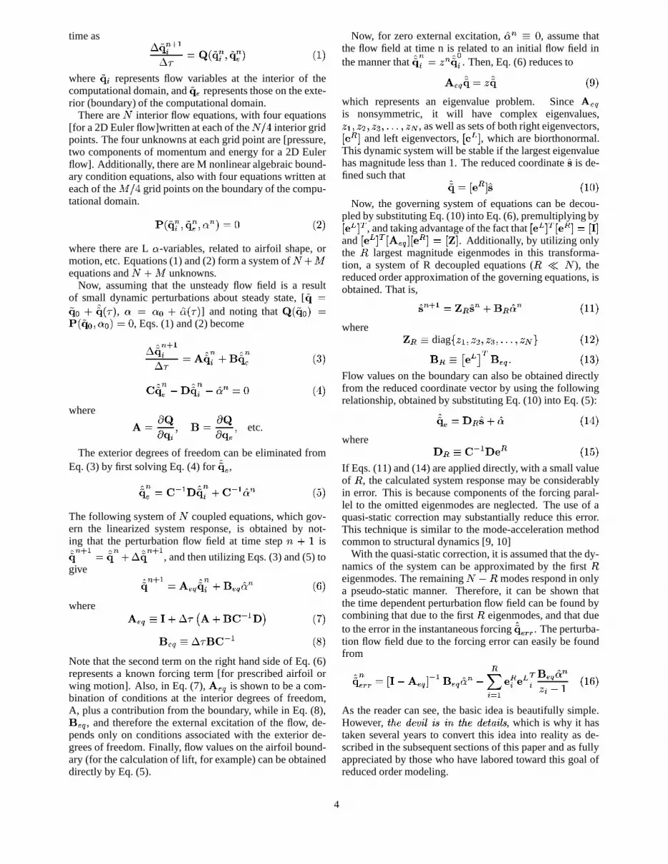
time as �2%������3��� 6 8;: 2%��3 < 2%�� > @ :�@

where 2%43 represents flow variables at the interior of thecomputational domain, and 2%?> represents those on the exte-rior (boundary) of the computational domain.

There are � interior flow equations, with four equations[for a 2D Euler flow]written at each of the � ��� interior gridpoints. The four unknowns at each grid point are [pressure,two components of momentum and energy for a 2D Eulerflow]. Additionally, there are M nonlinear algebraic bound-ary condition equations, also with four equations written ateach of the ����� grid points on the boundary of the compu-tational domain.

� : 2% �3 < 2% � > <�� � @ 6�� :�� @where there are L � -variables, related to airfoil shape, ormotion, etc. Equations (1) and (2) form a system of �����equations and ����� unknowns.

Now, assuming that the unsteady flow field is a resultof small dynamic perturbations about steady state, [ 2% 62%�� �"!2% : � @ , � 6#��� � !� : � @ ] and noting that 8 :12%���@ 6� : 2% � <�� � @ 6$� , Eqs. (1) and (2) become

� !2% ���%�3��� 6�& !2% �3 �(' !2% � > :*) @+ !2% � >�,.- !2% �3�, !�%� 6�� :/� @

where

& 60 80 %43 <1' 6

0 80 %?> < etc.

The exterior degrees of freedom can be eliminated fromEq. (3) by first solving Eq. (4) for !2% > ,

!2% � > 6 +32 � - !2% �3 � + 2 � !� � :�4 @The following system of � coupled equations, which gov-ern the linearized system response, is obtained by not-ing that the perturbation flow field at time step 56�7 is

!2% ����� 6�!2% � � � !2% �8��� , and then utilizing Eqs. (3) and (5) togive

!2% �8��� 6�& >9 !2% �3 �('�>:9 !� � :*; @where & >9=<$> � ��� ? &@�(' + 2 � -BA :DC @

'�>:9 < �E� ' + 2 � :*F @Note that the second term on the right hand side of Eq. (6)represents a known forcing term [for prescribed airfoil orwing motion]. Also, in Eq. (7), & >9 is shown to be a com-bination of conditions at the interior degrees of freedom,A, plus a contribution from the boundary, while in Eq. (8),' >9 , and therefore the external excitation of the flow, de-pends only on conditions associated with the exterior de-grees of freedom. Finally, flow values on the airfoil bound-ary (for the calculation of lift, for example) can be obtaineddirectly by Eq. (5).

Now, for zero external excitation, !� � < � , assume thatthe flow field at time n is related to an initial flow field inthe manner that !2% �3 6�G � !2% � 3 . Then, Eq. (6) reduces to

& >:9H!2%;6�G !2% :*I @which represents an eigenvalue problem. Since & >:9is nonsymmetric, it will have complex eigenvalues,G � <JG � <�G�K <MLNLNL <�G�O , as well as sets of both right eigenvectors,& ' ( * and left eigenvectors, & ')-�* , which are biorthonormal.This dynamic system will be stable if the largest eigenvaluehas magnitude less than 1. The reduced coordinate !P is de-fined such that !2%;6 & ' ( * !P ::M� @

Now, the governing system of equations can be decou-pled by substituting Eq. (10) into Eq. (6), premultiplying by& ' -�*�. , and taking advantage of the fact that & ' -#*�. & ' ( *�6 & > *and & ' - * . & & >9 *"& ' ( * 6 & Q * . Additionally, by utilizing onlythe R largest magnitude eigenmodes in this transforma-tion, a system of R decoupled equations ( RTS � ), thereduced order approximation of the governing equations, isobtained. That is,

!P ����� 6�Q ( !P � �(' ( !� � ::8�@where Q ( < diag UVG � <�G � <JGVK<NLNLML�<JGVOXW ::V� @

' ( <"Y ' -[Z . ' >:9 L ::M) @Flow values on the boundary can also be obtained directlyfrom the reduced coordinate vector by using the followingrelationship, obtained by substituting Eq. (10) into Eq. (5):

!2% > 6 - ( !P � !� ::N� @where - ( < + 2 � - ' ( ::V4 @If Eqs. (11) and (14) are applied directly, with a small valueof R , the calculated system response may be considerablyin error. This is because components of the forcing paral-lel to the omitted eigenmodes are neglected. The use of aquasi-static correction may substantially reduce this error.This technique is similar to the mode-acceleration methodcommon to structural dynamics [9, 10]

With the quasi-static correction, it is assumed that the dy-namics of the system can be approximated by the first Reigenmodes. The remaining � , R modes respond in onlya pseudo-static manner. Therefore, it can be shown thatthe time dependent perturbation flow field can be found bycombining that due to the first R eigenmodes, and that dueto the error in the instantaneous forcing !2% >]\J\ . The perturba-tion flow field due to the forcing error can easily be foundfrom

!2% � >]\J\ 6 & > , & >9 * 2 � ' >:9 !� � , (^3`_ �

' (3 ' - .3 ' >9 !� �G�3 , ::M; @As the reader can see, the basic idea is beautifully simple.However, ! 0 � �1� ��� �ba ��� ! 0 � ��! � ���ca , which is why it hastaken several years to convert this idea into reality as de-scribed in the subsequent sections of this paper and as fullyappreciated by those who have labored toward this goal ofreduced order modeling.

4

C. Eigenmode Computational MethodologyFor the simpler (lower dimensional) fluid models, say

a two-dimensional vortex lattice model of unsteady flowabout an airfoil, the size the eigenvalue matrix is of theorder 100 � 100. For such matrices, standard eigenvalueextraction numerical procedures may be used. We haveused EISPACK, an algorithm and computer code availablein most computational centers in the United States.

For more complicated fluid models, e.g., the full potentialmodels or Euler models the order of the eigenvalue matrixmay be in the range of 1000 to 10,000 squared or greater.For matrices of this size, new developments in eigenvalueextraction have been required. We have used methods basedupon the Lanczos algorithm. For the full potential equa-tion ( � V�8� ��� M� �8� ) an efficient and effective algorithmis described by Hall, Florea, and Lanzkron [4]. For theEuler equations ( � V� ��� M� � ), the paper by Dowell andRomanowski[7] will be of interest. The discussion of Ma-hajan et al. [5] is also recommended to the reader. As the ex-tensions to three-dimensional and viscous flows are made,further developments in eigenvalue and eigenmode deter-mination will likely be required or desired.

These further developments appear doable, but theamount of work should not be underestimated. Perhaps anappropriate use of primitive modes may be of help. Thatis, it may be possible to use the eigenmodes from a simplerfluid model as primitive modes for a more advanced fluidmodel. Much work remains to be done here.

A final and important point that Mahajan [5] has empha-sized is that the eigenvalue problem may be formulated ineither discrete or continuous time. The former allows eigen-value extraction from existing CFD codes using pre- andpost processor formats; thereby saving the considerable ef-fort of recoding existing CFD codes.

D. Proper Orthogonal Decomposition (POD)Modes

Romanowski [17] has given a clear discussion of this ap-proach and we follow his description here.

Given the difficulty of extracting eigenmodes for veryhigh dimensional systems, e.g., greater than 10 � , it is ofgreat interest to note that a simpler modal approach is avail-able as recently developed by Romanowski [17]. This ap-proach adapts a methodology from the fields of nonlineardynamics and signal processing, the POD or KL modal rep-resentation. See Ref. [17] for an introduction to the relevantliterature in these fields.

Here, we quote Romanowski’s account of the essence ofthe method.

Karhunen-Loeve Decomposition (KL Decomposition)[also called proper orthogonal decomposition (POD)] hasbeen used for a broad range of dynamic system character-ization and data compression applications. The procedure,which is briefly summarized below, results in an optimalbasis for representing the given data ensemble.

The instantaneous flow field vector,� 2%���� , is retained at

discrete times, such that 6# <J� <�)#<NLNLML�< . A carica-ture flow field,

� 2%��� � , is defined as the deviation of eachinstantaneous flow field from the mean flow field,

� 2% � of

the ensemble. � 2% � ��� < � 2% � � , � 2% � ::�C @A matrix &� �* is formed as the ensemble of the two pointcorrelation of the caricature flow fields, such that

���� � 6

� 2% � ��� .�� � 2% ���� ::MF @References [10] and [12] (of Ref. [17]) show that solvingthe eigenvalue problem

&� *8U�� W 6�� U�� W ::MI @produces an optimal set of basis vectors, U�� W 6U�� � <�� � <�� K <NLNLML�<�� � W for representing the flow field ensem-ble. Additionally, the magnitude of the eigenvalue, � � givesa measure of the participation of the th KL eigenvector inthe ensemble. Therefore, a reduced set of basis vectors caneasily be found by limiting the set to only those KL eigen-vectors corresponding to sufficiently large eigenvalues.”

Since the number of time steps and thus the order of thematrix needed to compute a reasonable and useful set of KLmodes is on the order of a few hundred, the determination ofKL modes is computationally very inexpensive, especiallyas compared to determining the eigenmodes of the originalfluid dynamics model. In the subsequent section results us-ing KL modes are shown to be in excellent agreement withthose obtained from the full order model and also the re-duced order model based upon eigenmodes. It also mightbe noted that one can first use the KL decomposition to re-duce the order of the original model and then do a furthereigenmode analysis of the reduced order model, a techniquethat may be useful for some applications.

As a final comment on the POD or KL methodology, it isimportant to note that a similar calculation may be done inthe frequency domain by assuming simple harmonic solu-tions and replacing the data at discrete time steps with dataat discrete frequencies over a frequency interval of inter-est. Kim [18] has used the POD frequency domain methodfor a vortex lattice fluid model and Thomas, Hall and Dow-ell [19, 20] have done so for an Euler fluid model includingshock waves at transonic conditions.

E. Balanced ModesBaker, Mingori, and Goggin [21] have used this method-

ology originally developed in the controls community todevelop reduced order aerodynamic models. Rule, Cox andClark [22] have explored this method as well and we largelyfollow their discussion here.

To determine the ���#! ������� ��� ��!�� � � ������ � � � a , the eigen-value problem of the original fluid model or its equivalentmust still be solved. The authors of Ref. [21] make the pointfor the example treated by them that the number of ���#! ��������������!�� � ������� � � � a needed for a given level of accuracyin a reduced order model may be less than the correspond-ing number of eigenmodes. They do confirm the results ofHall[2] for a potential fluid flow that a modal representationis computationally effective and accurate.

Rule, Cox and Clark [22] have also studied the internalbalancing approach and made a number of useful obser-vations. As these authors have noted, “Balanced realiza-tion is based upon the idea that a similarity transformation

5

exists which renders the controllability and observabilityGramian matrices of the system diagonal and equal. Statesin the transformed space are ordered by [their] importanceas transmission paths between system inputs and outputs.Values along the diagonal of the transformed Gramian ma-trix indicate the relative contribution of each state to theoutputs of interest, and provide a simple criterion for ei-ther retaining or neglecting states to form a reduced ordermodel.

Aerodynamic systems provide an ideal opportunity forthe application of balanced realization techniques, becauseit is frequently the case that a large number of states mustbe used to transmit information from a small number of in-puts (system geometry, control surface position), to a smallnumber of outputs (net lift, moment about the elastic axis).This is especially the case with CFD schemes which requirethe computation of two or three components of velocity pluspressure and density at thousands of nodes around a body,only to obtain a few integrated forces. From this view point,the details of the flow are unimportant; the aerodynamicsare simply providing a transmission path from geometry toforces.” They further comment that, “A detailed descriptionof an algorithm to find the balancing transformation, R, canbe found in Ref. [23]. Note that the computational cost offinding this transformation is � :*� K @ , which is comparablein cost to finding the eigenvalues and eigenvectors of thesame system. This becomes impractical for large systems,but efforts are being made to develop more efficient meth-ods of determining the most dominant states only [24].”

In comparing the relative merits of using eigenmodes ver-sus balanced modes, the authors make the following point.“Eigenvalues and eigenvectors are related to the internal dy-namics of the mathematical [CFD] model, and not to thephysical input/output mapping between airfoil geometricstates and integrated forces. Thus, the rationale for retain-ing or discarding modes is somewhat arbitrary [in an eigen-mode analysis]; in this case [the example treated by the au-thors of Ref. [22] the most lightly damped modes were re-tained. Heavily damped modes play an important role incalculating transient system response, which accounts forthe poor performance of the eigenmode method [relative tobalanced modes] in this limit [of short times or high fre-quency].”

All results to date for balanced modes have used a vor-tex lattice model, but in principle other CFD models can betreated in a similar fashion.

F. Synergy Among the Modal MethodsIn light of the above discussion, the following methodol-

ogy appears to be a practical and perhaps even an optimumapproach. With a given CFD model, a set of POD modescan be constructed of the order of 10

�to 10 K . Then using

the POD modes and the corresponding reduced order model(POD/ROM), further reduction may be obtained by extract-ing eigenmodes or balanced modes from the POD/ROM.For some applications where the smallest possible model isdesired, e.g. design for active control of an aeroelastic sys-tem, this further reduction will be desirable and perhaps es-sential using an eigenmode or balanced mode ROM. How-ever for validation studies where the identification and un-

derstanding of the most critical modes for stability is theprimary issue, one may prefer to retain a POD/ROM or aneigenmode ROM.

G. Input/Output ModelsThere is a long tradition of developing aerodynamic

transfer function representations from numerical data forsimple harmonic motion dating from the time of R.T. Jones’approximation to the Theodorsen function. Much of the rel-evant literature is summarized by Karpel [25] whose owncontribution was to develop a state-space or transfer func-tion representation of minimum order for a given level ofaccuracy using transfer function ideas based upon data forsimple harmonic motion. Hall, Thomas, and Dowell [19]have recently discussed such models in the light of the morerecent developments in aerodynamic modal representations.We follow their discussion here. See Ref. [9] and [25] forreferences to the original literature.

“Investigators have developed a number of techniquesto reduce the complexity of unsteady aerodynamic mod-els. R.T. Jones approximated indicial lift functions withseries of exponentials in time. Such series have particu-larly simple Laplace transforms, i.e. rational polynomialsin the Laplace variable s, making them especially usefulfor aeroelastic computations. Pad approximants are rationalpolynomials whose coefficients are found by least-squarescurve fitting the aerodynamic loads computed over a rangeof frequencies. Vepa, Edwards, and Karpel developed var-ious forms of the matrix Pad approximant technique. Thisapproach reduces the number of so-called augmented statesneeded to model the various unsteady aerodynamic trans-fer functions (lift due to pitching, pitching moment due topitching, etc.) by requiring that all the transfer functionsshare common poles.

...[A POD or eigenmode model] is similar in form to thatobtained using a matrix Pad approximant for the unsteadyaerodynamics ... and has some of the same advantagesof the Pad approach. Both methods produce low degree-of-freedom models. Furthermore, both require the aero-dynamic lift and moment transfer functions to share com-mon eigenvalues (although the zeros are obviously differ-ent). This is appealing because physically the poles shouldbe independent of the type of transfer function. However,the present [modal] approach has several advantages overthe matrix Pad approximant method. The present methodattempts to compute the actual aerodynamic poles, or atleast the poles of a rational CFD model. The Pad approach,on the other hand, selects pole locations by some form ofcurve fitting [of aerodynamic data for simple harmonic mo-tion]. In fact, some Pad techniques can produce unstableaerodynamic poles, even for stable aerodynamic systems.”

It is interesting to note that the notion of a transfer func-tion can be extended to nonlinear dynamical systems wherethe counterpart is usually called a describing function. Uedaand Dowell [26] pioneered and discussed this approach.

In the time domain, transfer functions can be invertedto form convolution integrals. Silva [27] has recently pi-oneered the extension of these ideas to nonlinear aerody-namic models using the concept of a Volterra integral.

6

H. Structural, Aerodynamic, and AeroelasticModes

Structural modes have a long and rich tradition. The nov-elty of much that is being discussed in the present paper isto extend these ideas to aerodynamic flows which also pos-sess a modal character, albeit a more complex one. Andfinally there are aeroelastic modes one may consider.

For the determination of structural modes, one normallyneglects dissipation or damping and thus only models ki-netic energy (or inertia) and potential strain energy (or stiff-ness). The eigenvalues are real (the natural frequenciessquared) as are the corresponding eigenmodes. Physicallyif one excites the structure with a simple harmonic oscil-lation at a frequency near that of an eigenvalue, the struc-ture will perform a simple harmonic oscillation at that samefrequency whose spatial distribution is given by the corre-sponding eigenvector.

For aerodynamic modes (and also for aeroelastic modes)the physical interpretation as well as the mathematical de-termination of the eigenvalues and eigenvectors or eigen-modes is more subtle and difficult, but still rewarding! Firstof all the eigenvalues are complex with real and imaginaryparts of the eigenvalue giving the oscillation frequency andrate of growth or decay (damping) of the eigenmode. As fora structural mode, if one is clever enough to excite only asingle aerodynamic eigenmode then an oscillation will oc-cur whose spatial distribution is given by the correspondingeigenvector. However the eigenvalues of an aerodynamicflow are closely spaced together, typically much closer thanthe eigenvalues for structural modes. Indeed if the aerody-namic computational domain were extended to infinity theeigenvalues would no longer be discrete but rather form acontinuous distribution for most aerodynamic flows. Thusexciting only a single aerodynamic mode experimentallyis a difficult feat. For some turbomachinery flows withbounded flows between blades in a cascade, discrete well-spaced eigenvalues are possible that have a resonant char-acter. This is also true for some aerodynamic eigenmodesin a wind tunnel, of course. And these have been observedexperimentally.

Aeroelastic modes are those that exist when the struc-tural and aerodynamic modes are fully coupled, i.e. oscil-lations of a fluid mode excite all structural modes and viceversa. In general these aeroelastic modes also have com-plex eigenvalues and eigenvectors. At low speeds (well be-low the flutter speed, for example) one may usually identifythe structural and aerodynamic eigenvalues separately sincethe structural/aerodynamic coupling is weak. However asthe flutter speed is approached, the eigenvalues may changesubstantially and the modes are more strongly coupled. Itis even possible for a mode that is aerodynamic in originat low speeds to become the critical flutter mode at higherspeeds, although normally it is one or more of the struc-tural modes that becomes unstable as the flow of velocityapproaches the flutter speed.

Winther, Goggin and Dykeman [28] have suggested usingaeroelastic modes to reduce the total number of modes to beused in a simulation of overall aircraft motion. This seemslike an idea worth exploring, although aeroelastic modes bydefinition vary with flow condition, e.g. dynamic pressure

and Mach number, and thus the aeroelastic modes at oneflight condition will not be the aeroelastic modes at another.Of course, if one uses a sufficient number of aeroelasticmodes they will be able to describe accurately the systemdynamics at any flight condition, but that tends to defeat thepurpose of minimizing the number of modes in the repre-sentation.

Also it should be noted that the particular implementationof aeroelastic modes in Ref. [28] does ���! include aerody-namic states or modes per se, which limits that particularapproach when the aerodynamic modes themselves are ac-tive and couple strongly with the structural modes. This isprobably the exceptional case, but it can happen.

III. ResultsIn an earlier summary of work and results on this

topic [1], we have discussed 1) comparisons of the reducedorder model to classical unsteady incompressible aerody-namic theory, 2) reduced order calculations of compressibleunsteady aerodynamics based on the full potential equation,3) reduced order calculations of unsteady flow about an iso-lated airfoil based on the Euler equations, 4) reduced ordercalculations of unsteady viscous flows associated with cas-cade stall flutter, and 5) linear flutter analyses using reducedorder model.

In the present paper, recent results for transonic flowswith shock waves including viscous and nonlinear effectsare emphasized. Before turning to these however, we con-sider some fundamental results concerning the effects ofspatial discretization and a finite computational domain.

A. The Effects of Spatial Discretization and aFinite Computational Domain

For simplicity we use a classical CFD model, the vortexlattice method for an incompressible potential fluid, to il-lustrate the points we wish to make. Compressible potentialflow models and Euler flow models have provided numer-ical results consistent with those obtained from the vortexlattice models in this regard. The results discussed here arefrom Heeg and Dowell [29].

In CFD there are two approximations that are nearly uni-versal to all such models. One is the construction of a com-putational grid that determines the limits of spatial resolu-tion of the computational model. The second is the approx-imation of an infinite fluid domain by a finite domain. It is aprincipal purpose of the present discussion to note that thecomputational grid not only determines the spatial resolu-tion obtainable by the CFD model, but also the frequencyor temporal resolution that can be obtained. Further, as willbe shown, the finiteness of the computational domain de-termines the resolution of the eigenvalue distribution fora CFD model. Both of these observations have importantramifications for assessing the CFD model and its abilityto provide an adequate approximation to the original fluidmodel on which it is founded as well as being helpful inconstructing and understanding reduced order models.

In the following discussion we shall consider both dis-crete time as well as continuous time eigenvalues. Even ina high dimensional system such as usually encountered withCFD, the relationship between any dynamical variable such

7

–1 –0.9 –0.8 –0.7 –0.6 –0.5 –0.4 –0.3 –0.2 –0.1 0–80

–60

–40

–20

0

20

40

60

80

Imag

Par

t of E

igen

valu

e, λ

Real Part of Eigenvalue, λ

Baseline1/2 as many wake elements

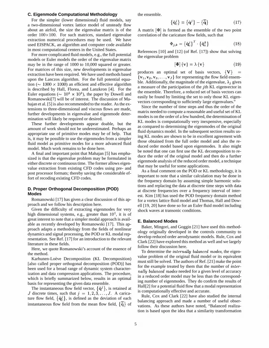
Figure 1: Influence of varying the size of the aerodynamicelements of vortex-lattice model. Continuous time eigen-values, � .

as vortex strength, velocity potential, flow velocity, density,pressure, etc. and its time evolution as expressed for thedetermination of eigenvalues and eigenvectors is a simpleone. For a given dynamic variable, % , which changed withtime, � , the eigenvalue relationship is

% 6�������� :D��� @where � is the continuous eigenvalue. For a discrete timerepresentation where the time step is

�� , we define the dis-

crete time eigenvalue, G , as the ratio of % to its value onetime step earlier. It is easily seen then that

G�6� ��� :D� �@or

� 6���� �:�G @J� � � :D�8� @It will be useful in our discussion to consider both � and G .

Here we use the vortex lattice model, because 1) it is oneof the simplest CFD models, 2) it has been widely used and3), among practitioners, it is thought to be well understoodin terms of its capability and limitations. As noted earlier,similar results are obtained from more elaborate CFD mod-els which include the effects of flow compressibility, rota-tionality and/or viscosity.

As an example, we consider the flow over an airfoil witha certain number of vortex elements on the airfoil and in thewake. Initially, we select 20 elements on the airfoil and 360elements in the wake. The finite length of the wake extends18 chord lengths. The eigenvalues and eigenmodes of theflow can be computed by now well-established methods.

The eigenvalue distribution for � is shown in Fig. 1. Notethat the real part of the eigenvalue is the damping and theimaginary part is the frequency of the eigenvalue. We nowstudy the effects of 1) refining the grid or vortex lattice spac-ing and 2) changing the extent of the wake length. Note thatin Fig. 1, the baseline configuration’s eigenvalue with thelargest imaginary part has a value of 10 � . If we now halvethe number of grid points or double the grid spacing, whilemaintaining the same total wake length, the total number ofeigenvalues remains constant. The frequency range of the

–1 –0.9 –0.8 –0.7 –0.6 –0.5 –0.4 –0.3 –0.2 –0.1 0–80

–60

–40

–20

0

20

40

60

80

Imag

Par

t of E

igen

valu

e, λ

Real Part of Eigenvalue, λ

Baseline1/2 as many wake elements

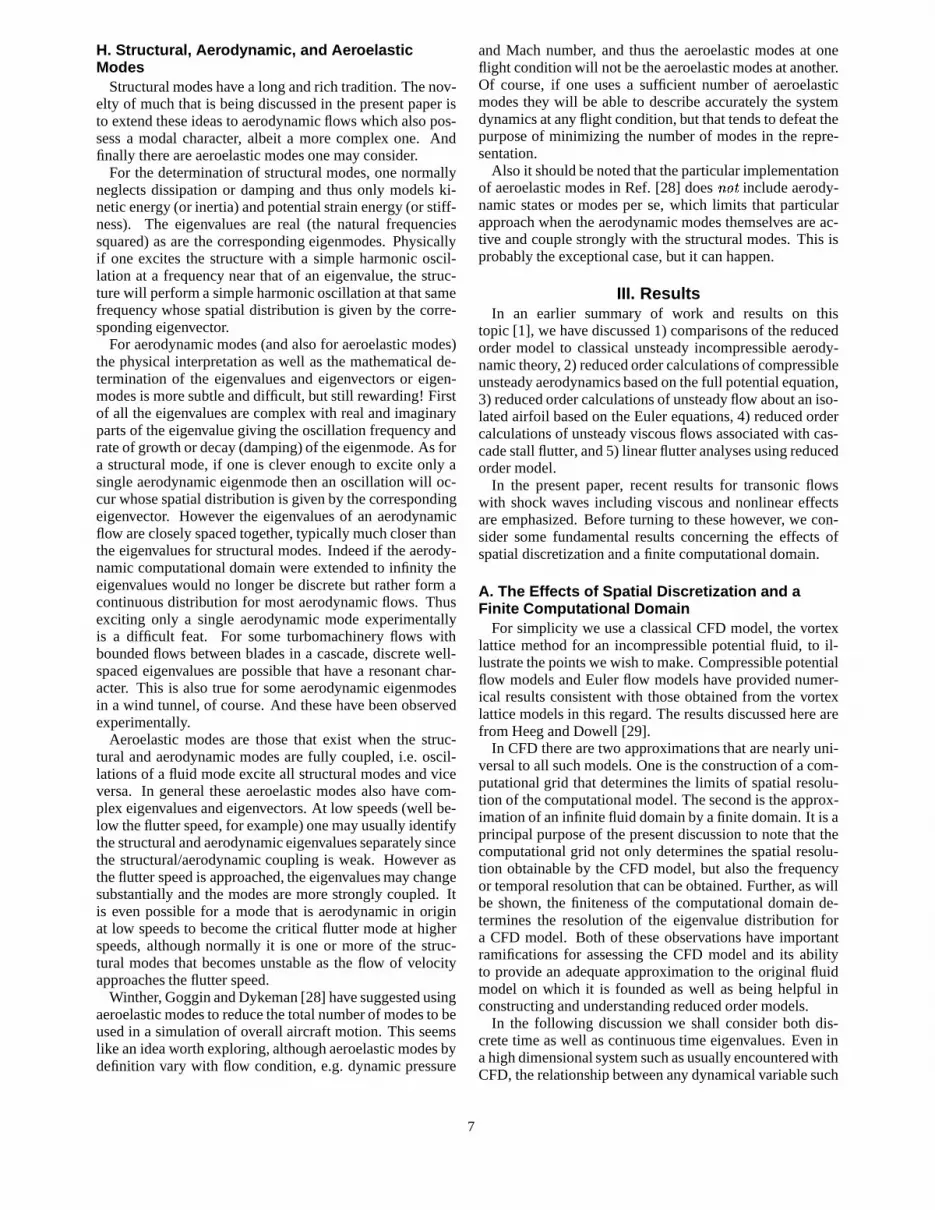
Figure 2: Influence of simultaneously varying the size andnumber of aerodynamic elements in the wake of vortex-lattice model, maintaining a constant wake length. Con-tinuous time eigenvalues, � .

original eigenvalues has doubled and the eigenvalues ex-hibit increased damping. Thus we see that refining the gridhas led to increasing the frequency range of the eigenvaluedistribution. By contrast the spacing of the eigenvalues inthe eigenvalue distribution is little changed by a change inthe computational grid spacing.

Now consider what happens as the extent of the wakelength is increased while the grid spacing is held constant.In Fig. 2, the baseline configuration is compared to an aero-dynamic model that has half as many aerodynamic elementsin the wake. Now we see the spacing between eigenvalueshas increased by about a factor of two, but the largest imag-inary part of the eigenvalue distribution (frequency) is un-changed. Hence, the effect of extending the wake length(for a fixed grid resolution) is to refine the resolution ofthe eigenvalue distribution, but not to change the maximumfrequency of the eigenvalue distribution. A more in depthinterpretation of this behavior is given in Heeg and Dow-ell [29] along with further details and numerical examples.

B. The Effects of Mach Number and Steady Angleof Attack: Subsonic and Transonic Flows

Here we examine some recent results from Thomas, Halland Dowell [19, 20] and also Florea, Hall and Dowell [30].The former used an Euler equation flow model with a fre-quency domain POD method and the latter a transonic po-tential flow model with a now standard eigenvalue, eigen-mode formulation. Although using different flow modelsand modal representations, the results of these two studieslead to similar conclusions regarding the nature of the flowand the efficacy of a modal representation of the aerody-namic flow.

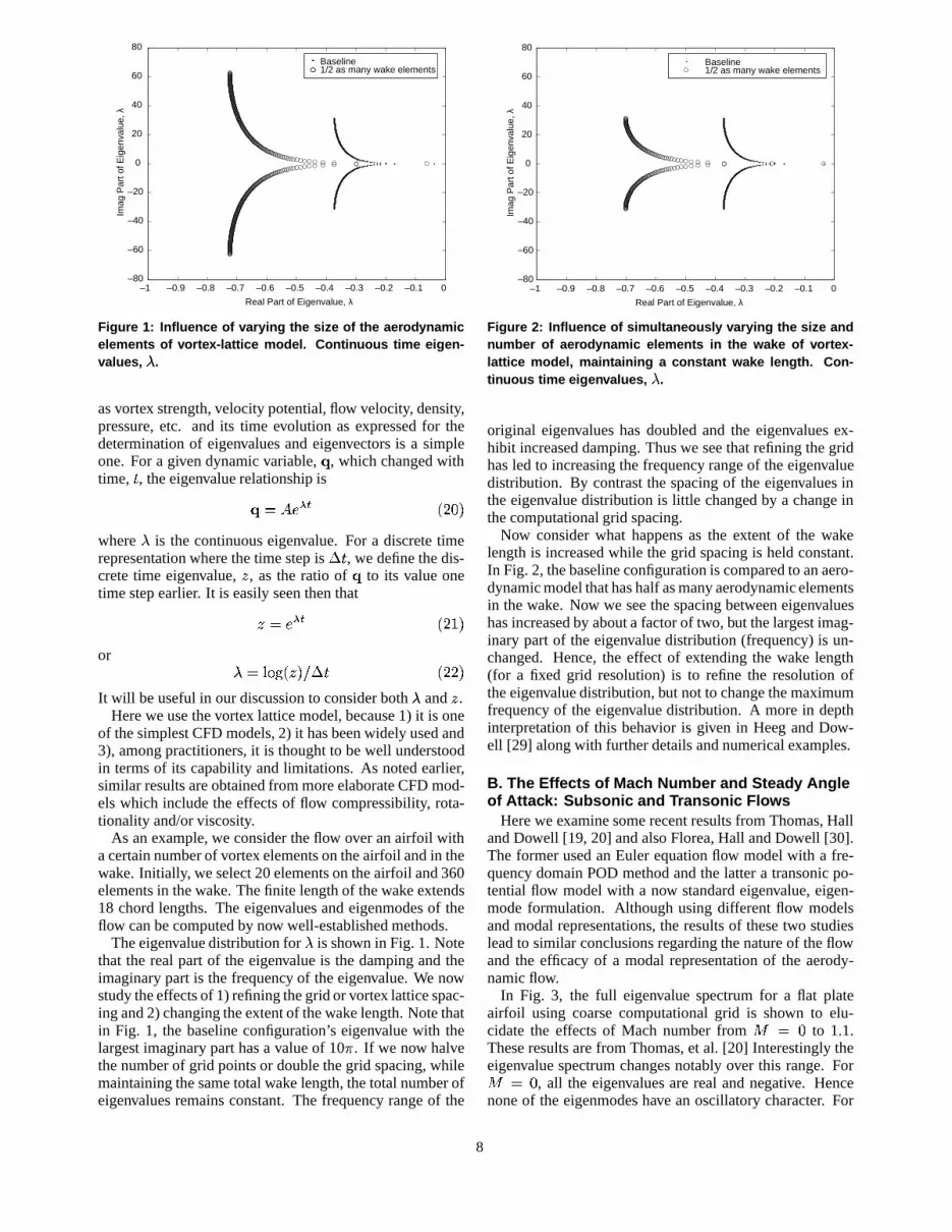
In Fig. 3, the full eigenvalue spectrum for a flat plateairfoil using coarse computational grid is shown to elu-cidate the effects of Mach number from � 6 � to 1.1.These results are from Thomas, et al. [20] Interestingly theeigenvalue spectrum changes notably over this range. For� 6"� , all the eigenvalues are real and negative. Hencenone of the eigenmodes have an oscillatory character. For

8

−0.5 −0.3 −0.1 0.1−0.6

−0.4

−0.2

0.0

0.2

0.4

0.6M=0.8

−0.5 −0.3 −0.1 0.1−0.6

−0.4

−0.2

0.0

0.2

0.4

0.6

Im(λ)

M=0.4

−0.5 −0.3 −0.1 0.1−0.6

−0.4

−0.2

0.0

0.2

0.4

0.6M=0.0

−0.5 −0.3 −0.1 0.1

Re(λ)

−0.6

−0.4

−0.2

0.0

0.2

0.4

0.6M=0.9

−0.5 −0.3 −0.1 0.1−0.6

−0.4

−0.2

0.0

0.2

0.4

0.6M=0.5

−0.5 −0.3 −0.1 0.1−0.6

−0.4

−0.2

0.0

0.2

0.4

0.6M=0.1

−0.5 −0.3 −0.1 0.1−0.6

−0.4

−0.2

0.0

0.2

0.4

0.6M=1.0

−0.5 −0.3 −0.1 0.1−0.6

−0.4

−0.2

0.0

0.2

0.4

0.6M=0.6

−0.5 −0.3 −0.1 0.1−0.6

−0.4

−0.2

0.0

0.2

0.4

0.6M=0.2

−0.5 −0.3 −0.1 0.1−0.6

−0.4

−0.2

0.0

0.2

0.4

0.6M=1.1

−0.5 −0.3 −0.1 0.1−0.6

−0.4

−0.2

0.0

0.2

0.4

0.6M=0.7

−0.5 −0.3 −0.1 0.1−0.6

−0.4

−0.2

0.0

0.2

0.4

0.6M=0.3

Figure 3: Full aerodynamic eigenspectrums. Flat-plate airfoil (16 � 8 mesh).

any Mach greater than zero, however, eigenvalues that arecomplex conjugate appear along with real eigenvalues. Theeigenvalue pattern continues to evolve as the Mach num-ber increases, with another significant change in characterin the transonic range from � 6 � L I to 1.1. The corre-sponding eigenmodes have also been determined includingthe characteristic pressure distributions on the airfoil. Typ-ically the eigenmode that corresponds to the smallest neg-ative real eigenvalue has a pressure distribution similar tothat for steady flow at a constant angle of attack.

As an aside, it is very interesting to note that the eigenval-ues for � 6 � are distributed along the real axis in Fig. 3,while in Fig. 1 they are distributed along the imaginary axis.In both cases these represent discrete approximations to abranch cut. It is well known from Theodorsen’s theory for� 6 � that the branch cut can be placed along any lineemanating from near the origin of the complex plane. Theresults of Fig. 1 and Fig. 3 indicate that different CFD mod-els for the same physical flow may place this branch cutalong distinctly different rays from the origin.

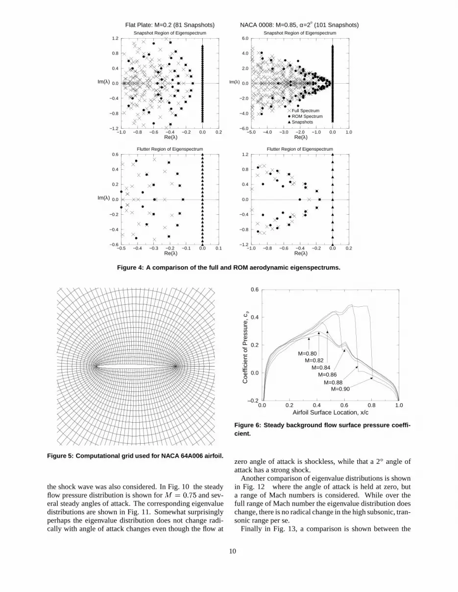
In Fig. 4, results are shown for a flat plate at � 6�� Lc� and0.9 and a NACA 0008 airfoil at � 67� L F 4 . For the latter,a shock is present. Results are shown for a finer mesh typi-cal of CFD calculations and results are shown from the fulleigenspectrum and those eigenvalues of the flow obtainedusing 100 POD modes to construct a reduced order model(ROM). The POD modes were determined using solutionsat discrete values, often called “snapshots” in the POD liter-ature, computed at uniformly distributed frequencies in the

range , 8L ��� Im : ��@�� L � . The dominant eigenmodesare well approximated by the POD/ROM model. Note thecharacteristic distribution of the eigenvalues as a functionof Mach number including with and without shock.

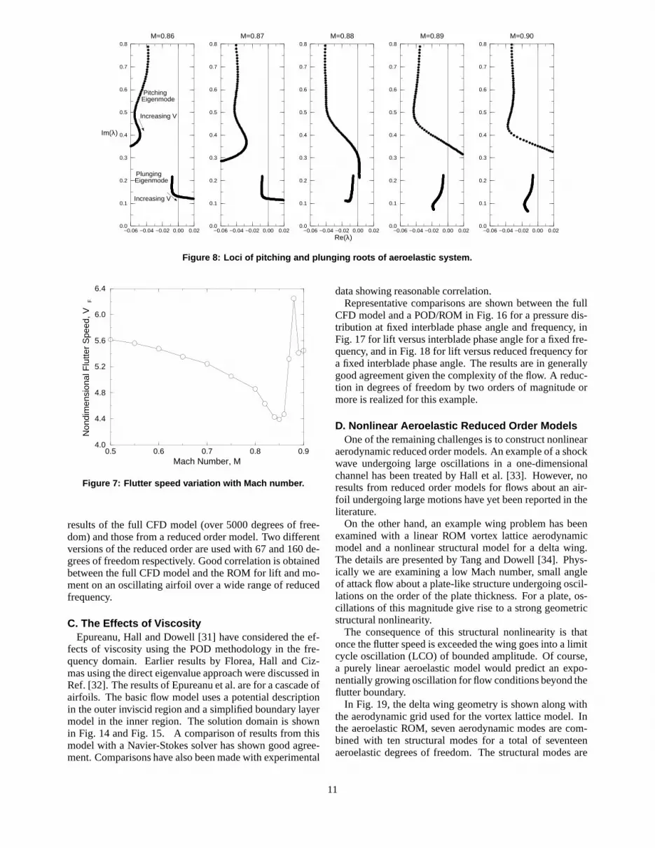
Further results have been obtained for a NASA 64A006airfoil. The CFD grid is shown in Fig. 5 and the steadyflow pressure distribution is shown in Fig. 6. Note a shockis distinctly present for � � � L F8; . For this airfoil abending/torsion flutter analysis is conducted over the Machnumber range � 6 � Lc4 to 0.9. The flutter boundary isshown in Fig. 7. Root loci for the two dominant aeroe-lastic modes (which originate in the plunging and pitch-ing structural modes at low Mach number) are shown inFig. 8 for Mach numbers in the range � 6 � L F8; to 0.9.These root loci show that, in the Mach number range wherethe position of the shock on the airfoil moves appreciably,the critical eigenmode for flutter changes from the plung-ing mode to the pitching mode. There is a correspondingand sharp change in the flutter boundary, c.f. Fig. 8. One ofthe benefits of a reduced order modal representation of theaerodynamic flow is the capability and ease of construct-ing such root loci which provide a significantly improvedunderstanding of transonic flutter.

We now turn to some complementary results from Florea,et al. [30] who have studied a NACA 0012 airfoil and aMBB A3 airfoil. We present results for only the formerairfoil here.

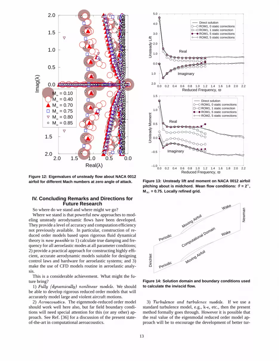
The grids used for the CFD models are shown in Fig. 9.In addition to the basic grid, a refined grid in the vicinity of

9

−0.5 −0.4 −0.3 −0.2 −0.1 0.0 0.1Re(λ)

−0.6

−0.4

−0.2

0.0

0.2

0.4

0.6

Im(λ)

Flutter Region of Eigenspectrum

−1.0 −0.8 −0.6 −0.4 −0.2 0.0 0.2Re(λ)

−1.2

−0.8

−0.4

0.0

0.4

0.8

1.2

Im(λ)

Flat Plate: M=0.2 (81 Snapshots)Snapshot Region of Eigenspectrum

−1.0 −0.8 −0.6 −0.4 −0.2 0.0 0.2Re(λ)

−1.2

−0.8

−0.4

0.0

0.4

0.8

1.2Flutter Region of Eigenspectrum

−5.0 −4.0 −3.0 −2.0 −1.0 0.0 1.0Re(λ)

−6.0

−4.0

−2.0

0.0

2.0

4.0

6.0

Im(λ)

NACA 0008: M=0.85, α=2o (101 Snapshots)Snapshot Region of Eigenspectrum

Full SpectrumROM SpectrumSnapshots

Figure 4: A comparison of the full and ROM aerodynamic eigenspectrums.

Figure 5: Computational grid used for NACA 64A006 airfoil.

the shock wave was also considered. In Fig. 10 the steadyflow pressure distribution is shown for � 6 �HLcC84 and sev-eral steady angles of attack. The corresponding eigenvaluedistributions are shown in Fig. 11. Somewhat surprisinglyperhaps the eigenvalue distribution does not change radi-cally with angle of attack changes even though the flow at

0.0 0.2 0.4 0.6 0.8 1.0Airfoil Surface Location, x/c

–0.2

0.0

0.2

0.4

0.6

Coe

ffici

ent o

f Pre

ssur

e, c

p

M=0.80M=0.82

M=0.84

M=0.90M=0.88

M=0.86

Figure 6: Steady background flow surface pressure coeffi-cient.

zero angle of attack is shockless, while that a 2 � angle ofattack has a strong shock.

Another comparison of eigenvalue distributions is shownin Fig. 12 where the angle of attack is held at zero, buta range of Mach numbers is considered. While over thefull range of Mach number the eigenvalue distribution doeschange, there is no radical change in the high subsonic, tran-sonic range per se.

Finally in Fig. 13, a comparison is shown between the

10

−0.06 −0.04 −0.02 0.00 0.020.0

0.1

0.2

0.3

0.4

0.5

0.6

0.7

0.8

Im(λ)

M=0.86

−0.06 −0.04 −0.02 0.00 0.020.0

0.1

0.2

0.3

0.4

0.5

0.6

0.7

0.8M=0.87

−0.06 −0.04 −0.02 0.00 0.02Re(λ)

0.0

0.1

0.2

0.3

0.4

0.5

0.6

0.7

0.8M=0.88

−0.06 −0.04 −0.02 0.00 0.020.0

0.1

0.2

0.3

0.4

0.5

0.6

0.7

0.8M=0.89

−0.06 −0.04 −0.02 0.00 0.020.0

0.1

0.2

0.3

0.4

0.5

0.6

0.7

0.8M=0.90

Pitching

Increasing V

Increasing V

Plunging

Eigenmode

Eigenmode

Figure 8: Loci of pitching and plunging roots of aeroelastic system.

0.5 0.6 0.7 0.8 0.9Mach Number, M

4.0

4.4

4.8

5.2

5.6

6.0

6.4

Non

dim

ensi

onal

Flu

tter

Spe

ed, V

F

Figure 7: Flutter speed variation with Mach number.

results of the full CFD model (over 5000 degrees of free-dom) and those from a reduced order model. Two differentversions of the reduced order are used with 67 and 160 de-grees of freedom respectively. Good correlation is obtainedbetween the full CFD model and the ROM for lift and mo-ment on an oscillating airfoil over a wide range of reducedfrequency.

C. The Effects of ViscosityEpureanu, Hall and Dowell [31] have considered the ef-

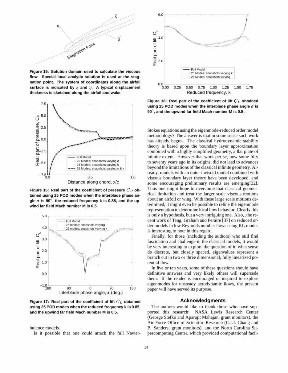
fects of viscosity using the POD methodology in the fre-quency domain. Earlier results by Florea, Hall and Ciz-mas using the direct eigenvalue approach were discussed inRef. [32]. The results of Epureanu et al. are for a cascade ofairfoils. The basic flow model uses a potential descriptionin the outer inviscid region and a simplified boundary layermodel in the inner region. The solution domain is shownin Fig. 14 and Fig. 15. A comparison of results from thismodel with a Navier-Stokes solver has shown good agree-ment. Comparisons have also been made with experimental

data showing reasonable correlation.Representative comparisons are shown between the full

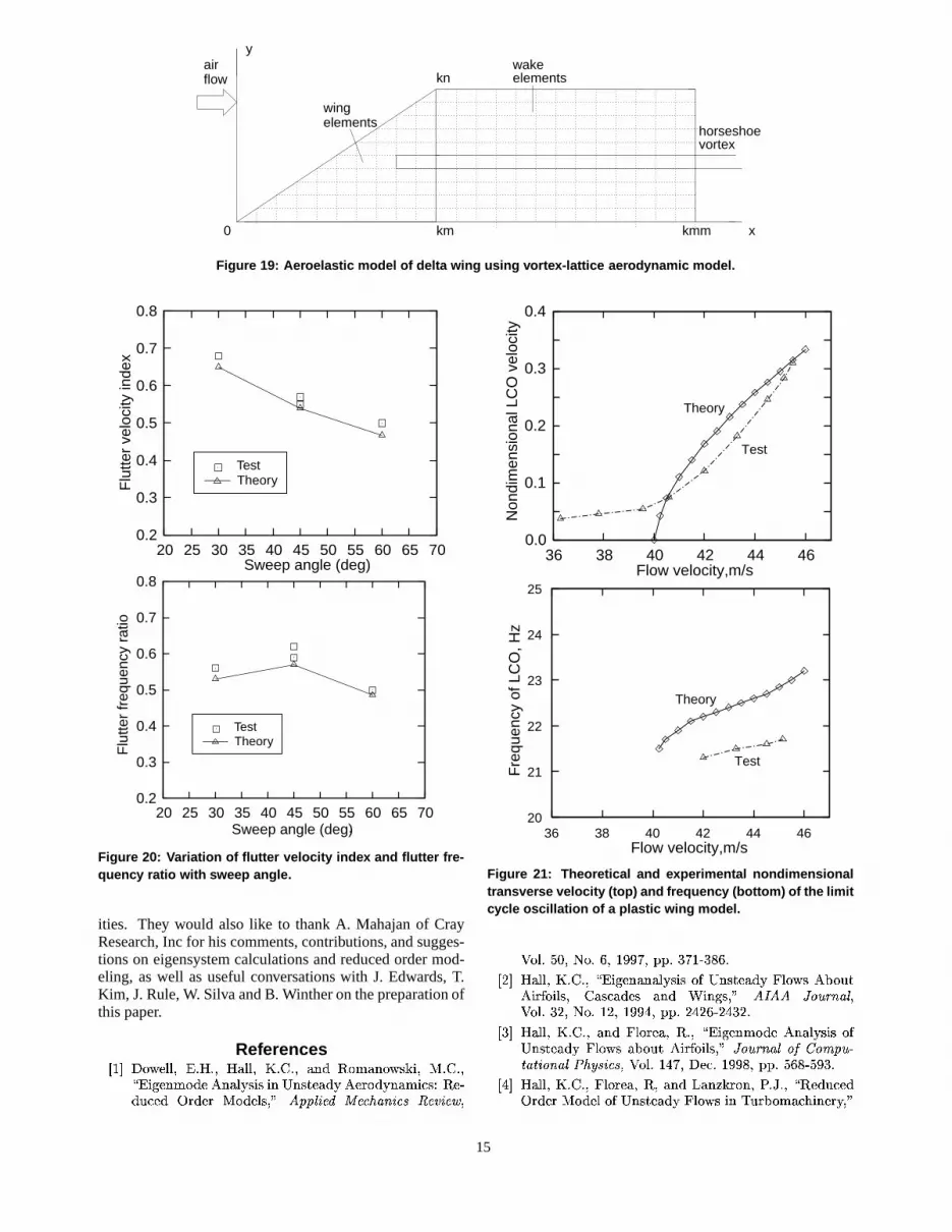
CFD model and a POD/ROM in Fig. 16 for a pressure dis-tribution at fixed interblade phase angle and frequency, inFig. 17 for lift versus interblade phase angle for a fixed fre-quency, and in Fig. 18 for lift versus reduced frequency fora fixed interblade phase angle. The results are in generallygood agreement given the complexity of the flow. A reduc-tion in degrees of freedom by two orders of magnitude ormore is realized for this example.

D. Nonlinear Aeroelastic Reduced Order ModelsOne of the remaining challenges is to construct nonlinear

aerodynamic reduced order models. An example of a shockwave undergoing large oscillations in a one-dimensionalchannel has been treated by Hall et al. [33]. However, noresults from reduced order models for flows about an air-foil undergoing large motions have yet been reported in theliterature.

On the other hand, an example wing problem has beenexamined with a linear ROM vortex lattice aerodynamicmodel and a nonlinear structural model for a delta wing.The details are presented by Tang and Dowell [34]. Phys-ically we are examining a low Mach number, small angleof attack flow about a plate-like structure undergoing oscil-lations on the order of the plate thickness. For a plate, os-cillations of this magnitude give rise to a strong geometricstructural nonlinearity.

The consequence of this structural nonlinearity is thatonce the flutter speed is exceeded the wing goes into a limitcycle oscillation (LCO) of bounded amplitude. Of course,a purely linear aeroelastic model would predict an expo-nentially growing oscillation for flow conditions beyond theflutter boundary.

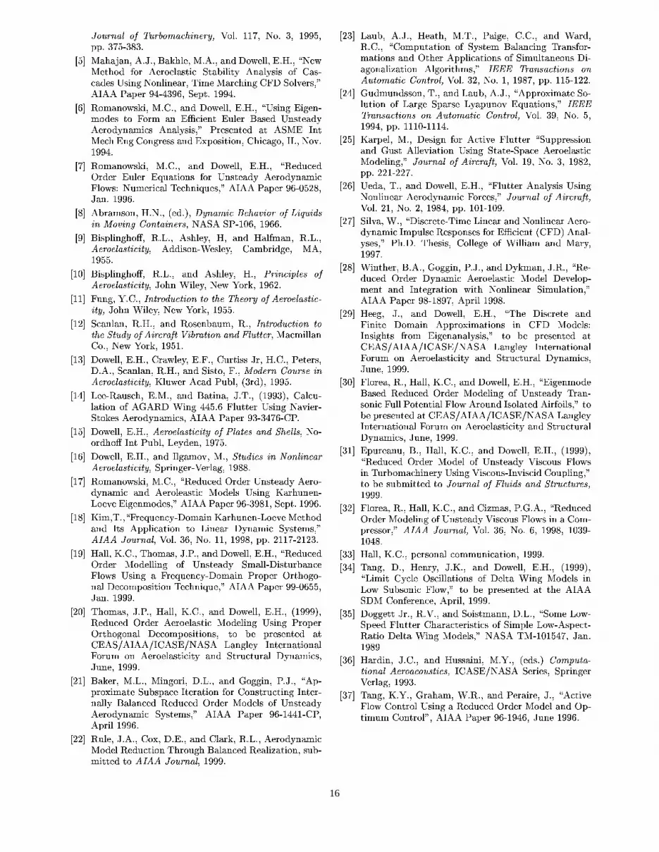
In Fig. 19, the delta wing geometry is shown along withthe aerodynamic grid used for the vortex lattice model. Inthe aeroelastic ROM, seven aerodynamic modes are com-bined with ten structural modes for a total of seventeenaeroelastic degrees of freedom. The structural modes are

11

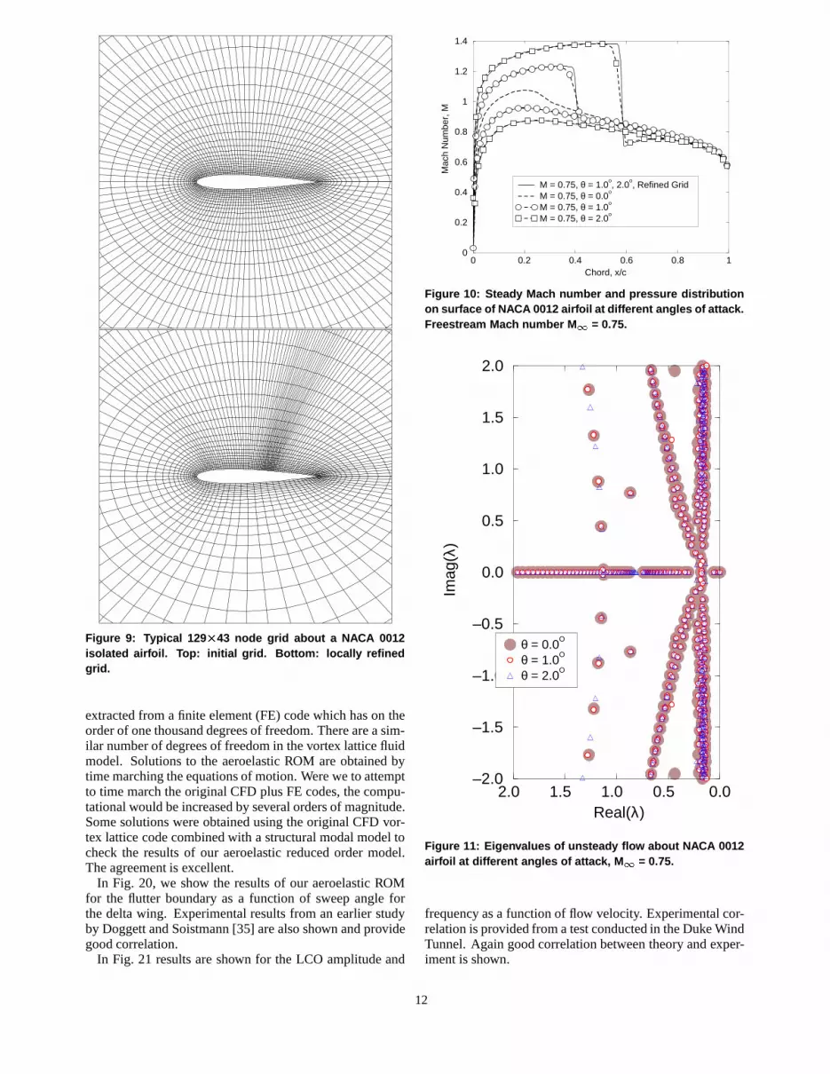
Figure 9: Typical 129 � 43 node grid about a NACA 0012isolated airfoil. Top: initial grid. Bottom: locally refinedgrid.

extracted from a finite element (FE) code which has on theorder of one thousand degrees of freedom. There are a sim-ilar number of degrees of freedom in the vortex lattice fluidmodel. Solutions to the aeroelastic ROM are obtained bytime marching the equations of motion. Were we to attemptto time march the original CFD plus FE codes, the compu-tational would be increased by several orders of magnitude.Some solutions were obtained using the original CFD vor-tex lattice code combined with a structural modal model tocheck the results of our aeroelastic reduced order model.The agreement is excellent.

In Fig. 20, we show the results of our aeroelastic ROMfor the flutter boundary as a function of sweep angle forthe delta wing. Experimental results from an earlier studyby Doggett and Soistmann [35] are also shown and providegood correlation.

In Fig. 21 results are shown for the LCO amplitude and

0 0.2 0.4 0.6 0.8 1Chord, x/c

0

0.2

0.4

0.6

0.8

1

1.2

1.4

Mac

h N

umbe

r, M

M = 0.75, θ = 1.0o, 2.0

o, Refined Grid

M = 0.75, θ = 0.0o

M = 0.75, θ = 1.0o

M = 0.75, θ = 2.0o

Figure 10: Steady Mach number and pressure distributionon surface of NACA 0012 airfoil at different angles of attack.Freestream Mach number M � = 0.75.

2.0 1.5 1.0 0.5 0.0Real(λ)

–2.0

–1.5

–1.0

–0.5

0.0

0.5

1.0

1.5

2.0

Imag

(λ)

θ = 0.0O

θ = 1.0O

θ = 2.0O

Figure 11: Eigenvalues of unsteady flow about NACA 0012airfoil at different angles of attack, M � = 0.75.

frequency as a function of flow velocity. Experimental cor-relation is provided from a test conducted in the Duke WindTunnel. Again good correlation between theory and exper-iment is shown.

12

2.0 1.5 1.0 0.5 0.0Real(λ)

2.0

1.5

1.0

0.5

0.0

0.5

1.0

1.5

2.0

Imag

(λ)

M∞ = 0.10 M∞ = 0.40 M∞ = 0.70 M∞ = 0.75 M∞ = 0.80 M∞ = 0.85

Figure 12: Eigenvalues of unsteady flow about NACA 0012airfoil for different Mach numbers at zero angle of attack.

IV. Concluding Remarks and Directions forFuture Research

So where do we stand and where might we go?Where we stand is that powerful new approaches to mod-

eling unsteady aerodynamic flows have been developed.They provide a level of accuracy and computation efficiencynot previously available. In particular, construction of re-duced order models based upon rigorous fluid dynamicaltheory is ��� � � � aJa�� !�� � to 1) calculate true damping and fre-quency for all aeroelastic modes at all parameter conditions;2) provide a practical approach for constructing highly effi-cient, accurate aerodynamic models suitable for designingcontrol laws and hardware for aeroelastic systems; and 3)make the use of CFD models routine in aeroelastic analy-sis.

This is a considerable achievement. What might the fu-ture bring?

1)��� ������� � ���� ����� ��� ��� ��� �#� ������� �7� � ���ca� We should

be able to develop rigorous reduced order models that willaccurately model large and violent aircraft motions.

2) �1��� � ��� � a�! ��� a� The eigenmode-reduced order modelshould work well here also, but far field boundary condi-tions will need special attention for this (or any other) ap-proach. See Ref. [36] for a discussion of the present state-of-the-art in computational aeroacoustics.

0.0 0.2 0.4 0.6 0.8 1.0 1.2 1.4 1.6 1.8 2.0 2.2Reduced Frequency, ω

2.0

1.0

0.0

1.0

2.0

3.0

4.0

5.0

Uns

tead

y Li

ft

Direct solutionROM1, 0 static correctionsROM1, 1 static correctionROM1, 5 static correctionsROM2, 5 static corrections

Real

Imaginary

0.0 0.2 0.4 0.6 0.8 1.0 1.2 1.4 1.6 1.8 2.0 2.2Reduced Frequency, ω

–1.0

–0.5

0.0

0.5

1.0

1.5

Uns

tead

y M

omen

t

Direct solutionROM1, 0 static correctionsROM1, 1 static correctionROM1, 5 static correctionsROM2, 5 static corrections

Imaginary

Real

Figure 13: Unsteady lift and moment on NACA 0012 airfoilpitching about is midchord. Mean flow conditions: � = 2 � ,M � = 0.75. Locally refined grid.

Computational Domain

Diri

chle

t

New

man

Periodic

Periodic

Wake

Wake

Moving Airfoil

Moving Airfoil

Figure 14: Solution domain and boundary conditions usedto calculate the inviscid flow.

3) � � ��! � � �1����� ��� ! � ��! � � ������� � � �1�ca� If we use astandard turbulence model, e.g., k- , etc., then the presentmethod formally goes through. However it is possible thatthe real value of the eigenmodal reduced order model ap-proach will be to encourage the development of better tur-

13

η

ξ

Stagnation Pointδ∗

Figure 15: Solution domain used to calculate the viscousflow. Special local analytic solution is used at the stag-nation point. The system of coordinates along the airfoilsurface is indicated by � and � . A typical displacementthickness is sketched along the airfoil and wake.

0.0 0.5 1.0Distance along chord, x/c

–7.5

–5.0

–2.5

0.0

2.5

5.0

7.5

Rea

l par

t of p

ress

ure,

CP

Full Model25 Modes; snapshots varying σ25 Modes; snapshots varying k25 Modes; snapshots varying σ & k

Figure 16: Real part of the coefficient of pressure ��� ob-tained using 25 POD modes when the interblade phase an-gle � is 90 � , the reduced frequency k is 0.85, and the up-wind far field Mach number M is 0.5.

180 90 0 90 180Interblade phase angle, , (deg.) σ

–1.0

0.0

1.0

2.0

3.0

4.0

5.0

Rea

l par

t of l

ift, C

L

Full Model25 modes; snapshots varying s25 modes; snapshots varying k

Figure 17: Real part of the coefficient of lift � - obtainedusing 25 POD modes when the reduced frequency k is 0.85,and the upwind far field Mach number M is 0.5.

bulence models.Is it possible that one could attack the full Navier-

0.00 0.25 0.50 0.75 1.00 1.25 1.50 1.75Reduced frequency, k

0.0

2.0

4.0

6.0

Rea

l par

t of l

ift, C

L

Full Model25 Modes; snapshots varying k25 Modes; snapshots varying s

Figure 18: Real part of the coefficient of lift � - obtainedusing 25 POD modes when the interblade phase angle � is90 � , and the upwind far field Mach number M is 0.5 .

Stokes equations using the eigenmode-reduced order modelmethodology? The answer is that in some sense such workhas already begun. The classical hydrodynamic stabilitytheory is based upon the boundary layer approximationcombined with a highly simplified geometry, a flat plate ofinfinite extent. However that work per se, now some fiftyto seventy years ago in its origins, did not lead to advancesbeyond the limitations of the classical infinite geometry. Al-ready, models with an outer inviscid model combined withviscous boundary layer theory have been developed, andsome encouraging preliminary results are emerging[32].Thus one might hope to overcome that classical geomet-rical limitation and treat the larger scale viscous motionsabout an airfoil or wing. With these large scale motions de-termined, it might even be possible to refine the eigenmoderepresentation to determine local flow behavior. Clearly thisis only a hypothesis, but a very intriguing one. Also, ,the re-cent work of Tang, Graham and Peraire [37] on reduced or-der models in low Reynolds number flows using KL modesis interesting to note in this regard.

Finally, for those (including the authors) who still findfascination and challenge in the classical models, it wouldbe very interesting to explore the question of in what sensedo discrete, but closely spaced, eigenvalues represent abranch cut in two or three dimensional, fully linearized po-tential flow.

In five or ten years, some of these questions should havedefinitive answers and very likely others will supersedethem. If the reader is encouraged or inspired to exploreeigenmodes for unsteady aerodynamic flows, the presentpaper will have served its purpose.

AcknowledgmentsThe authors would like to thank those who have sup-

ported this research: NASA Lewis Research Center(George Stefko and Aparajit Mahajan, grant monitors), theAir Force Office of Scientific Research (C.I.J. Chang andB. Sanders, grant monitors), and the North Carolina Su-percomputing Center, which provided computational facil-

14

wing

horseshoevortex

wakeelements

elements

yairflow

km

kn

xkmm0

Figure 19: Aeroelastic model of delta wing using vortex-lattice aerodynamic model.

0.2

0.3

0.4

0.5

0.6

0.7

0.8

20 25 30 35 40 45 50 55 60 65 70

Flu

tter

velo

city

inde

x

Sweep angle (deg)

TestTheory

0.2

0.3

0.4

0.5

0.6

0.7

0.8

20 25 30 35 40 45 50 55 60 65 70

Flu

tter

freq

uenc

y ra

tio

Sweep angle (deg).

TestTheory

Figure 20: Variation of flutter velocity index and flutter fre-quency ratio with sweep angle.

ities. They would also like to thank A. Mahajan of CrayResearch, Inc for his comments, contributions, and sugges-tions on eigensystem calculations and reduced order mod-eling, as well as useful conversations with J. Edwards, T.Kim, J. Rule, W. Silva and B. Winther on the preparation ofthis paper.

References������������ � ������ ���������� � ������ �������! #"%$&�(')�! *��+-,/.���01� �����2 �3.�4(�5 *'��6"*�87� #�! :9/+-.�+;.� =<> #+@?A�5�("/9�7���BA�6"69/ C�!'�.�D5+5EF$&��G"*H*D5�"JI�BK"/��BL0M�6"/�5 �+5� NPORQSQUT VXW-Y%Z[W-\K]*^!_#V�\�`ba&W�cV�W�de�

0.0

0.1

0.2

0.3

0.4

36 38 40 42 44 46

Non

dim

ensi

onal

LC

O v

eloc

ity

Flow velocity,m/s

Theory

Test

20

21

22

23

24

25

36 38 40 42 44 46

Fre

quen

cy o

f LC

O, H

z

Flow velocity,m/s

Theory

Test

Figure 21: Theoretical and experimental nondimensionaltransverse velocity (top) and frequency (bottom) of the limitcycle oscillation of a plastic wing model.

f �( ��Ug�h/�*i>�/�Cj6�k�l!lSmn�Co#oF�*pSm6��Gqp(r(j6�� s������ � ��F��� ����� 2 �3.�4!�5 C�� C�� �9/+-.�+=�!tR<> *+@?A��("69vuw ���+x7�yU�(H/?

7�.:B-tz�(.� �+5�P���!+-D5�("*��+{�� C"}|~.� *4(+5� N�O&�-O�O��6�!�6�K_U^(T �f �( ��Cp(s6�*i>�/�;�s6�k�5l(l��*�Uo*o;�#s��Ss!j�G�s��SpSsn�

� p������� � ��e��� �������� C"�uw ��!BA��6�R$x��� 2 �3.�4!�5 #'��6"/�M7& C�� �9/+-.�+���t<> *+@?A��("69�uw ���+���yU�(H/?�7&.�B-tz�(.� �+5� N~�6�!�6��_C^(T��@�v�e�!��QC�/�� ^ � V���_U^(TC�R]6��`AV�\�`A� f �! ��;���nm6�#���5D(�F�l!l(r6�Uo#oF�Cg�j(r�G@g�l(p6�

� �������� � ��F��� �����Fuw ��!BA��6�k$x���! #"��k�! *�5,nBA�( F�F��� �*��� 2 $&�"/H#D5�"I�BK"*��B�0M�6"*�� U�!t;<> #+@?A�5�("/9�uw ���+�.� ��kH*BAyU�!')�!DK�#.� #��B-9n� N

15

�6�!�6�K_U^(Tx�@���#�6���A�!��^S\K]6V _UW������ f �( ��=�!��m6��i>�*�&p6���l!lSgn�o#oF�*pSm(gGqp(r(p6�

� g��0 �!�#���@�! F�S7x� �/�����R�!,6�# ��(�(01� 7����!�! #"������5 � ��!��� ����� 2 i>��0M��?A�*�6" t �!B~7���BA�n�� ��+@?A.�D�n?K�!y#.� �.:?�9 7� C�� :9*+-.�+b�!t1���!+@GD�!"*�5+�<�+-.� *4�i��( * �.� *���B�S��.�'���0 ��BADK�#.� #4���uw��/�! ��S��BA+5� N7� �7>7 ���!oU��B�l��!GX�Sp!l(j/���/�5o/?�F�5l(l��*�

� j���$&�(')�! *��+-,/.��U01� �����F�� C" ������ � ��F��� ����� 2 <�+-.� #4��e.�4!�5 *G'��6"*��+M?A� u*�!BA' �� %����D5.��5 n? �3H# ���B�����+-�" <� #+@?A��!"/97���BA�6"/9/ C��'�.�D�+~7� #�! :9/+-.�+5� N �3BA��+-�5 n?A�" ��? 7��*0 �� � n?0M�5DK�x�e *4��R�( #4�BA�5+-+��� C"=���*oU�!+-.:?A.��! ;�S�R�#.�D��4(�*�� @�3�5i����U��l!l!�/�

� m��$&�(')�! *��+-,/.�� 01� �����b�! #" ������ � ������ ����� 2 $&�"/H#D5�"I�BK"*��B �3H# ���B����nHC��?A.��! #+[tz�!B <� #+@?A��!"/9 7&��BA�6"/9/ C��'�.�Duw ���+5E3i>H#'���BA.�D5�! C�;�5D��* #.��nH#�5+5� N�7� �7>7~����oU��B�l!j�GqhSg!s!r6��S�� ;�F�l(l!j/�

� r��)7�y/BK�!'�+-�! ;�/��� i��������"F� �����=��_U^!��V�\ �>WA]*^!cV���������!�V#"��6V�Y!`V _MZ1��cV _%$v�e�!_ � ^!Vz_�W��K`K�#i�7 �*7&�*��GK�5h(j6�k�l!j(j6�

� l��'�R.�+-o# �.� #4!�#��(��)$�� �e���)7&+-�# ���9n�������! #" ���! :tz')�! ;��$�� �3���O�W��@��W�T�^!` � V�\�V � ��� 7>"*"*.�+-�( /GX|[�5+- ���9n� ���!'�y/BA.�"*4(�!� 0 7���l(g(gn�

�:�h��'�R.�+-o# �.� #4!�#��(���$�� �e������ C" 7&+-�# ���9n������� ���KV _C\�V QUT�W�`%�@�O�W��@��W�T�^!` � V�\�V � �����(�!�# M|L.� ���9n�/i>��*)8�!BA,U���l!jSsn�

�:�(���)u#H* #4*��)�� �����*�K_ � �-�Y!�*\ � V��!_ � � � ]#W+�;]#W-�!�����@�RO�W��@��W�T�^!` � V�\5�V � �����(�!�# M|L.� ���9n�*i>��)8�!BA,U���l(g(g6�

�:��s�,�/D5�! # ��� ;��$x� �������� C"b$&�(+-�� /y#�!H*' �R$x���&�K_ � �@�Y!�*\ � V��!_ � �� ]#W.- � �*Y!���@��O&Vz�-\��-^�� �0/ V#���@^ � V��!_�^!_UY21RT � ��� W��K�n0 ��D5'�.� � �� �R�*���#i>��)8�!BA,U���lSgn�(�

�:�p��������� � ��#��� �����#�8BK�5� ���9n�#��� uR���U�RH/B-?A.�+-+���B�*��� �����#�w��?A��BA+5���� 7����3�6D�! * ��! ;�/$x� �����6�! #",�/.�+@?A�*�/uR���#Z1�YnW��K_��e�!�6�K`�W�Vz_O�W��@��W�T�^!` � V�\�V � ���U�= �Hn���B�7�D5�("M�3H#y* ��4��p�BK"5���F�l(l(g6�

�:�5���)�;����GX$>��H#+-DK�;�8��� 01������ C"�����?A.� #�/���/� �>��� �@�l(l!p6�������! �D5H*G ���?A.��( [�!t�787�7�$&� |~.� *4 �(�Sg6� jvuw �H*?-?A��B�<�+-.� *4Mi>���6.���B-G�6?A�!,S�5+�7&��BA�6"/9/ C��'�.�D5+5�*7� @7�7%����oU��B�l(p�Gqp��nm!j�G������

�:��g�������� � ������ �����;O&W��-��W�T�^!` � V�\�V � �M�@�>��T�^ � W�`�^�_UY,-6]#W�T T `A�Ci��!G�!BK"/�#��(9 � n?&�eH*y# ��#�;��9*"*�� ;���l(m(g6�

�:�j��������� � ��;��� �����w�� C": � �4S��'������;01���;- � �*Y!V�W�`�V _:<x��_CT V _UWA^��O�W��@��W�T�^!` � V�\�V � ���=�/o/BA.� #4(��B-G f ��BA ��!4/�;�5l(r!r/�

�:��m��$&�(')�! *��+-,/.��#01� ����� 2 $&�"/H#D5�"MI�BK"*��B�<� #+@?A��!"/9�7&��BA�!G"/9/ #�!'�.�D �� C" 7���BA�! ���!+@?A.�D 0M�6"*�� �+�<�+-.� *4%�x��BA�/H* #�5 /G�;�n�>�S�R�3.�4(�5 *'��6"*�5+5� N>7� @7�7����!oU��B�l(j�Gqp(l(r6�(�?�/�5o/?�(�l!l(j6�

�:�r����=.�' � �>��� 2 u*BA�@�nH#�5 *D�96GX���(')��.� x�x��BA�/H* #�5 /Gq�;�n���S�R0M��?A�*�6"�! #"A X?A+�7�o*o# �.�D��?A.��( ?A� �F.� *���B �>9/ #�!'�.�DB�n9/+@?A�5'�+5� NO&�-O�O �6���/�K_U^!T � f �( ��Cp!j/�*i>�/�;�!�(�k�5l(l!r/�Co*o;�Cs6�!��m�G�sn��s!p6�

�:�l������� � ��!��� �����(���*�(')��+5�S�*� �w���S�� C"=������ � ��(��� ����� 2 $&�"/H#D5�"I�BK"*��B 0M�6"*�5 � �.� #4 ��t <> *+@?A��("69C�/')�! � :GX��.�+@?AH*BAy#�! #D��uw ���+ <�+-.� #4~�bu*BA�@�nH#�� #D�96GX���(')��.� ��BA�(oU��B1I�B-?A�#�(4!�!G C�� C���5D��('�oU�(+-.:?A.��( )�;�5D��* #.��nH#�(� N�7� �7>7~����oU��B�l!l�Gqh(j(g(gn��S�� ;�F�l(l!l/�

� s!h��)���#�!')�!+5�3�/� �w���3���� � ��3��� �����e�! #"[������ � ��e��� �����2�@�l!l(lD���$&�"*H*D5�" I�BK"*��B 7&��BA�n�5 ��!+@?A.�D 0M�6"/�5 �.� *4~<>+-.� *4~��BA�(oU��BI�B-?A�#�!4(�! C�! %���5D5�!'�oU�(+-.:?A.��( #+5� ?A� yU�Po*BA��+-�5 n?A�" ��?���e7��FE�7� �7>7�E� -��7 �*�GE�i�7 �*7 �k�� #4! ���9H � n?A��BA #��?A.��( #�! u#��BAH#' �( 7&��BA�n�5 ��!+@?A.�D5.:?q9 �! #"I�6?-BAH*D�?AH*BK�� ��>9/ #�!'�.�D5+5��(H* #�(�F�l!l(l/�

� s6���'����,S��B�801� �e���R0M.� #4(��BA.��R��� �3���e�� C"J7>�!4(4!.� F���w� �*��� 2 7&o*Go*BA�@�/.�')��?A�+�6H#y#+-o#�!D5�K X?A��BK��?A.��! t �!B��R�( *+@?-BAH#D�?A.� *4L � n?A��B-G C�� � �9M���� �� #D5�5" $��5"*H#D��"~I�BK"/��B 0M�6"*�5 �+��!tx<� #+@?A��!"/97���BA�6"/9/ C��'�.�D�69/+@?A�5'�+5� N 78 @7�7}����oU��B l(j�GK���(�/��G����w�7�o/BA.� 3�5l(l!j/�

� s(s��$&H# ��(�*�*� 7����C�R�����/��� �����#�! #" �R ���BA,U�*$�� �3���*7&��BA�6"/9/ C��'�.�D0M�6"*�� /$&�"/H#D�?A.��( ����*BA�!H#4!�N���� �� #D5�5"�$&��! �.����?A.��! ;�n+-H*y*G'�.:?-?A�"�?A��O��-O&O �6�!�6�K_U^(T �;�l!l(l/�

� s!p��)�k��H#yF��7x� �*���������?A�F��01� �>�������!.�4(�(����� �������! #" | ��BK"F�$x� ����� 2 �R�!'�o#H/?K��?A.��( ~��tO�69/+@?A�5'P���� ��! #D�.� *4 �;BK�! *+@t �!B-G')��?A.��! #+��! C" I�?A�*��B�7&o#o* �.�D��?A.��( #+��!tQ�/.�'�H* :?K�! #���(H#+���.:G�!4!�( #�! �.����?A.��( 7� �4!�!BA.:?A�#'�+5� N{�SRGR�RT�*�-^!_*`�^(\ � V��!_#` ��_O&� � �!��^ � V�\)�e��_ � �-�!T � f �! ��#p(s6�*i>�/�F�!���l(r(m6�#o#o;�U�!��gGK�s(sn�

� s����,7>HC"/'�H* C"*+-+-�! ;�!�>���6�! #"��;�!H#yF�n7x� �/��� 2 7�o*o*BA�@�/.�')��?A�2�6�!G �H*?A.��( �!t=�k��BA4!�9�/o#��BA+-�v��96�!o*H# *�����G�nHC��?A.��( #+5� Nb�SR�RGR�#�@^!_#`�^S\ � V���_#`v��_bO&� � �!��^ � V�\ �e��_ � �-�!T � f �( ��ep!l/��i��*�8g6��l!l!�/�Co#oF�;�!�(�5h�GA�(�!�5�*�

� s(g���x��BAoU�� ���01�����>�5+-.�4( btz�!B 7�D�?A.��(�vuw �H*?-?A��B 2 �/H#o*o*BA�5+-+-.��! �! #"B7>H*+@?�7� � ����6. ��?A.��( L<>+-.� *4J�6?K��?A��GU�/o#�!D5�v7&��BA�n�5 ��!+@?A.�D0M�6"*�� �.� *4*� N��6�!�6�K_U^(Te�@��O&V �-\��@^@� � � f �( ��w�5l/�Fi>�/��p/�3�l!rSsn�o#oF�#s(s6��G�s(s(mn�

� s!j���<>�5"#�/�F�>���;�! #"v�����5 � ��;��� ����� 2 uw �H/?-?A��B=7& C�! :9/+-.�+�<>+-.� *4i>�! # �.� #���B=7&��BA�6"/9/ C��'�.�D�u*�!BAD5�5+5� N �6�!�6��_C^(Te�@�=O&Vz�-\��-^�� � �f �( ��Usn�(�*i>�/�Usn�k�l!r!�/�Co#oF���h/��GA�h(l6�

� s(m�,�/.� ��!�/��| ��� 2 ��.�+-D�BA��?A��Gq��.�'����;.� #�5��Be�! #"�i��( * �.� *���Be7&��BA�!G"/9/ #�!'�.�DG q'�o#H* �+-�8$���+-oU�( #+-��+3tz�!Be����D5.��5 n?8�X��uw�V�k7& C�! :G9/+-�5+5� NL�3�;� �������*�5+-.�+5�x�R�( � ��54!���!tx|L.� � �. ��' �� C" 0 ��B-9n��l!lSmn�

� s!r���|L.� n?A�#��B�6��� 7����37>�!4(4(.� F�#�w� �*���6�� C"��>9/,6')�! F�S�/� $x��� 2 $&��G"*H*D5�" I�BK"*��B��>9/ C��'�.�Db7&��BA�n�5 ��!+@?A.�D 0M�6"/�5 )�����S�5 ��!o*G'��5 n? �� C"A � n?A�54!BK��?A.��( �.:?A� i��( * �.� *���BM�/.�'�H# ���?A.��( F� N7� �7>7 ���!oU��B�l!r�GA�r!lSm6�U7�o*BA.� ��l!l(r6�

� s!l����>���54*�~�*���L�! #" �>��R�5 � ��L��� ����� 2 ���*� ��.�+-D�BA��?A� �! #"uw.� #.:?A� ���!')�!.� 7�o#o/BA�@�*.�')��?A.��! #+ .� ��uw� 0M�6"/�5 �+5E � *+-.�4(�n?A+ t BA�(' �e.�4(�� C�! #�! :9/+-.�+5� N ?A�JyU� o*BA�5+-�� 6?A�5" ��?���e7��FE�7� �7>7�E� -��7 �*�GE�i�7 �*7 �k�� #4! ���9H � n?A��BA #��?A.��( #�! u#��BAH#' �( 7&��BA�n�5 ��!+@?A.�D5.:?q9 �! #"I�6?-BAH*D�?AH*BK�� ��>9/ #�!'�.�D5+5��(H* #�(�F�l!l(l/�

� p(h��)uw ��!BA��6�/$����n�>�! � ��6��� �����/�� C"������� � ��*��� ����� 2 �3.�4(�5 *'��6"*�����+-�"L$��"/H#D5�5" I�BK"*��Bv0M�6"*�5 �.� #4 �!t�<> *+@?A��("69L�;BK�� *G+-�( *.�D�u#H# � n�w��?A�5 n?A.��! /uw ��� 7�BA�(H* C"K �+-�! ��?A�"�7&.:B-t �(.� �+5� N=?A�yU��o/BA�5+-�5 n?A�"���?8���87 �FE�7� @7�7�E� -��7��/�.E�i�7 �*7 �k�! *4( ���9 � n?A��BA #��?A.��( #�! Fu#��BAH#' �! 7&��BA�n�5 ��!+@?A.�D5.:?�9M�! #"W�n?-BAH#D�?AH/BK�! �>9/ C��'�.�D5+5�*�(H# *�(�;�5l(l!l/�

� p/���)�3o#H*BA�5�! 6H;�X���������� � ��3��� �����3�! #"[������ � ��e��� �����2�@�l!l(lD���2 $&�"/H#D5�" I�BK"/��B�0M�6"/�5 =�!t�<> *+@?A��("69 f .�+-D��(H#+ uw ���+.� ��;H*BAyU�(')��D��*.� #��B-9x<�+-.� *4 f .�+-D��(H#+@GY q 3�6.�+-D5.�"��R�(H#o* �.� *4*� N?A��yU��+-H#y#'�.:?-?A�"�?A�v�6�!�6��_C^(T3�@��1RT �6V�Y�`�^!_UY'- � �K�#\ � �6�-W�`K��l!l(l6�

� pSs�)uw ��!BA��6�n$x���(���� � ��(��� �����6�� C"��R.��5')��+5�n�w� 7�� 7���� 2 $&�"/H#D5�"I�BK"*��B80M�6"*�5 �.� #4=��t�<> #+@?A�5�("/9 f .�+-D5�(H*+Ruw ���+8.� ����R�('�Go*BA��+-+-�!B� N[O��-O&OJ�6�!�6�K_U^(T � f �( ��;p(j6��i>�/�kj6���l!l(r6���h!p(l�G�h��Sr6�

� p(p������� � ��*��� �����CoU��BA+-�! C�! ;D5�('�'�H# *.�D5��?A.��( F�F�5l(l!l/�� p!���)�w�� #4*�)�������>�5 /B-9n���*� ����� �! C" ���R�5 � ������ �����9�@�l!l(lD���

2 �F.�'�.�? �89/D5 ��1I>+-D5.� � ���?A.��! #+ ��t����5 :?K�[|L.� #4b0M�6"*�� �+ .� �;�Z�/H*y#+-�! #.�Dvuw ��=� N ?A��yU�vo*BA��+-�5 n?A�" ��?�?A�#��7� �7>7�/�=0 �R�( *tz��BA�5 *D5�(�U7&o*BA.� ��;�5l(l!l/�

� pSg�����!4(4(��?-?>��B���#$�� f ���*�� C"[�6�(.�+@?A')�! * ;�/��� �e��� 2 �/�!'��=�;��G�/oU���"vuw �H*?-?A��B=�R�C��BK��D�?A��BA.�+@?A.�D5+=�!t.�6.�'�o* ����F��G�7&+-oU�5D�?-G$���?A.��M���� �?K��|L.� #4 0M�6"*�5 �+5� Nvi�7 �*7 ��0 GA�h6��g��Sm6�3�(�! ;��l!r(l

� p(j�������BK"*.� ;���*� �����>�! C"~��H#+-+A��.� *.��=01� )����O���"*+5� ���e�!�>Q#� � ^!�� V��!_C^(TeO&W��-�^S\A�!�6` � V�\�`A�8 -��7��/�.E�i�7 �*7\�6��BA.��5+5�2�6o*BA.� #4!��Bf ��BA ��!4*�F�l!l(p6�

� pSm�)�w�� #4*����� )�����7�BK���C��' �U| � $����F�! #"��w��BK�!.:BA�(�;�*��� 2 7&D�?A.��S�uw �� �R�( n?-BA�( F<>+-.� #4���$&�"/H#D5�"�I�BK"/��B&0M�6"*�� k�� C" I>o*G?A.�'�H*' �R�( n?-BA�! �N/�U78 @7>7 ���!oU��B�l!j�GA�l��Sj/�U�(H# *���l!l(j/�

16