Reduced-order LQG control of a Timoshenko beam model · present numerical tests assessing the stability and performance of ... The theory of optimal feedback control ... Reduced-order

www.oeaw.ac.at

www.ricam.oeaw.ac.at

Reduced-order LQG controlof a Timoshenko beam model

Philipp Braun, Erwin Herńandez, DanteKalise

RICAM-Report 2015-08

Reduced-order LQG control of aTimoshenko beam model

Philipp Braun, Erwin Hernandez and Dante Kalise

Abstract. We present a computational approach for the construction of reduced-order controllers for the Timoshenko beam model. By means of a space discretiza-tion of the Timoshenko equations, we obtain a large-scale, finite-dimensionaldynamical system, for which we compute an LQG controller for closed-loop sta-bilization. The solutions of the algebraic Riccati equations characterizing theLQG controller are then used to construct a balancing transformation whichallows the dimensional reduction of the large-scale dynamic compensator. Wepresent numerical tests assessing the stability and performance of the proposedapproach.

Keywords. Timoshenko beam, closed-loop control, model order reduction, LQGcontrol/ balancing.

1. Introduction and description of the problem

The design of mechanisms for vibration control is a highly relevant topic in structuraldynamics (see for instance [17] and references therein). Among the different controlstrategies, model-based feedback control is widely used to generate a stable closed-loop that attenuates external dynamical disturbances. The underlying complexity ofthis optimal design problem motivates its mathematical and numerical analysis.

We approach the structural vibration problem by considering the well-acknowledgedTimoshenko beam model, describing the deformation of a beam of thickness τ over areference configuration Ω × (−τ/2, τ/2), where Ω := (0, L) with L the length of thebeam. The vibration is characterized in terms of the rotation amplitude θ(x, t) andthe transverse displacement amplitude w(x, t), both depending on the space variablex and the time variable t. For a clamped beam, the vibration is governed by the

2 P. Braun, E. Hernandez and D. Kalise

following second-order evolution system:

ρS∂2w

∂t2= kSG

(

∂2w

∂x2−

∂θ

∂x

)

+ u(x, t) + f(x, t) x ∈ Ω, t ∈ R+0 , (1)

ρI∂2θ

∂t2= EI

∂2θ

∂x2+ kSG

(

∂w

∂x− θ

)

x ∈ Ω, t ∈ R+0 , (2)

w(0, t) = w(L, t) = θ(0, t) = θ(L, t) = 0 t ∈ R+0 , (3)

w(x, 0) = w0(x),∂w

∂x(x, 0) = ζ(x) x ∈ Ω, (4)

θ(x, 0) = θ0(x),∂θ

∂x(x, 0) = η(x) x ∈ Ω. (5)

The coefficients ρ, E, and G, represent the mass density, the Young modulus and, theelasticity modulus of the shear, respectively. The coefficient k is a correction factorusually taken as 5/6. The parameters S and I represent the sectional area of thebeam and the inertia moment; in this case, considered as S = τ2 and I = τ4/12,respectively. The term f(x, t) accounts for external loads and disturbances, whereasthe control u(x, t) is assumed to be a constant load in space, distributed along a fixedsubset ωc of the domain,

u(x, t) = χωc(x)u(t)

where χωc(x) denotes the indicator function over ωc. The feedback control problem is

related to the computation of u(t) by means of a mapping K ∈ L([L2(Ω)]4,R) acting

over the current state of the system y = (w, θ, w, θ) (where henceforth ˙( ) stands fortime derivative)

u(t) = −Ky ,

such that external disturbances are compensated and the system is steered towardsa certain reference trajectory. However, in a realistic setting a full knowledge of thestate of the system is not available, and an additional observation equation

z(t) = Cy

with C ∈ L([L2(Ω)]4,Rm), is often considered. As a consequence, the feedback op-erator is evaluated over estimates p constructed from the measurements and theknowledge of the system dynamics,

u(t) = −Kp .

This paper concerns the study and numerical approximation of such a control loopover the infinite-dimensional dynamics defined by the Timoshenko model. The ap-proach that we follow considers in a first step a space discretization of the dynamicsleading to a large-scale dynamical system, to subsequently address the design prob-lem at a finite-dimensional level. The theory of optimal feedback control under partialinformation for linear, finite-dimensional systems is well understood and dates backto the seminal work by Kalman [11]. Feedback control design for infinite-dimensionalsystems following the aforementioned approach have been studied in several cases,e.g., [3, 6, 14]. In particular, similar problems for the Timoshenko model have been

Reduced-order LQG control of a Timoshenko beam model 3

studied in [18, 19, 9]. One drawback of the approach is the high complexity of theresulting controller, as the number of state space variables is directly linked to thediscretization parameters used in the first step. Furthermore, the computation of thecontroller/observer pair involves solving Riccati equations of the same order. Instead,we propose an intermediate step of model order reduction, allowing to approximatethe dynamics (and therefore the controller) by a considerably lower dimensional sys-tem. Model order reduction is a well-established technique for the simulation of con-trol of large-scale systems [4, 7], and has been successfully applied in the control ofinfinite-dimensional systems [1, 5, 8, 12]. In this paper we follow a linear quadraticGaussian control/reduction approach as presented in [15], where the reduction isobtained as a by-product of the computation of the feedback control.

The paper is structured as follows. In section 2, we present the abstract, infinite-dimensional setting and its numerical approximation via a locking-free finite elementformulation. In section 3, we address the finite-dimensional optimal control and es-timation problems by means of an LQG controller, which is then reduced using anad-hoc balanced truncation algorithm. Finally, in section 4 we present numericalexperiments illustrating the performance of the proposed approach.

2. The abstract setting and its approximation

In order to fit the problem within the classical settings of linear control theory, webegin by recasting eqns. (1)-(5) as a first-order evolution system. By considering theelastic operator

A(w, θ) := −

kGρ

∂2

∂x2 −kGρ

∂∂x

kAGρI

∂∂x

EI

∂2

∂x2 − kAGρI

w

θ

, D(A) = [H2(Ω) ∩H10 (Ω)]

2 ,

we can define the augmented operators (A,B)

A :=

[

0 I−A −D(A)

]

, B :=

00

χωc(x)0

,

where I corresponds to the identity operator. For sake of simplicity, henceforth weshall neglect the existence of disturbances (f ≡ 0), and thus reduce the problem tothe implementation of an optimal feedback regulation under partial state observation.With no additional difficulties, this can be modified in order to include the effect ofnoise. We have introduced a damping operator D(A), which in our case will be setas D(A) = αA, α > 0, as discussed in [13, Chapter 5]. We can now represent theTimoshenko model as the first-order linear system

y(x, t) = Ay +Bu , (6)

y(x, 0) = y0(x) (7)


acting over the state y = (w, θ, w, θ)T . We shall also consider the existence of anobservation equation

z = C(y) , (8)

where the observation operator C ∈ L([L2(Ω)]4 Rm) will be defined as

C(y)(t) :=

(

1

|ω1|

∫

ω1

w(x, t) dx, . . . ,1

|ωm|

∫

ωm

w(x, t) dx

)

,

where ωimi=1 are disjoint, non-empty subsets of Ω. Having defined the abstract state

space representation (6)-(8), we now turn our attention to the control design problem.We consider the state space Y = [H1

0 (Ω)]2 × [L2(Ω)]2 such that D(A) ⊂ Y , a control

space U = R, an observation space Z = Rm, and a cost functional

J(y, u) =1

2

∫

∞

0

‖z‖2Z + ‖u‖2U dt . (9)

The corresponding optimal control problem reads

minu∈L2([0,∞);R)

J(y(u), u) (10)

subject to system dynamics and observations (6)-(8). We present some relevant re-sults for this problem concerning the well-posedness of the optimal control problem(10). For more details concerning the abstract problem we refer to [9].

Proposition 2.1. A is the infinitesimal generator of a strongly continuous, analyticsemigroup eAt,on Y .

Proposition 2.2. (Finite cost condition) For every initial condition y0 ∈ Y , thereexists u ∈ L2([0,∞);R) such that J(y, u) < ∞.

Note that due to the inclusion of a damping term generates an exponential decay ofthe uncontrolled system, and therefore J(y, u) < ∞. Exponential stabilizability anddetectability follow trivially ([13]).

Theorem 2.3 ([9]). For each initial condition y0 ∈ Y, there exists a unique optimalpair (u∗, y∗) of the abstract optimal control problem subject to the system dynamics(6).

Formally, the solution of the optimal control problem (10) with partial observation(the LQG control problem) is expressed as a dynamic compensator of the form

y = Ay +Bu , (11)

z = Cy , (12)

p = (A−BK)p+ F (z − Cp) , (13)

u = −Kp , (14)

with

K = B∗P , F = QC∗ , (15)


where the operators P and Q ∈ L(Y, Y ) are the unique non-negative self-adjointoperators satisfying the following operator Riccati equations

A∗P + PA− PBB∗P + C∗C = 0 , (16)

AQ+QA∗ −QC∗CQ+BB∗ = 0 . (17)

Note that these are abstract operator equations over an infinite-dimensional statespace. In what follows, we shall generate an approximating sequence of finite-dimensionalstate-space representations (Ah, Bh, Ch), leading to approximate solutions (Ph,Qh)which converge to the solution of this abstract problem when h goes to 0. For thispurpose, the first step is to consider a discretization in space of the system leading toa finite-dimensional representation of the dynamics. In this context, the applicationof standard finite elements or finite difference schemes is usually sufficient to gen-erate a theoretically and computationally convergent sequence of problems (see forinstance, the series of examples in [13, Chapter 5]). However, it is well-known that theapplication of standard finite element approximations to the Timoshenko model leadsto the so-called locking-phenomenon, which produces unsatisfactory results when thebeam tichkness parameter τ is decreased [2]. In this latter reference, a locking-freemixed finite element formulation is proposed. The application of this technique forthe control problem (10) has been presented in [9], and we adopt a similar approach.We briefly recall the most relevant steps in the locking-free discretization.

Let us consider a finite-dimensional approximating subspace Vh ⊂ H10 (Ω), to be a

piecewise linear finite element space. For this reason, we consider a family Th ofregular partitions of the interval Ω:

Th : 0 = x0 < x1 < · · · < xn = L,

with mesh size h := L/n. The subspace Vh can be written as

Vh :=

v ∈ H10 (Ω) : v|[xj−1−xj ] ∈ P1, j = 1, . . . , n

⊂ H10 (Ω).

Let Vh1consists of the elements of Vh and equipped with the H1(Ω) seminorm and

let Vh2consists of the elements of Vh equipped with the L2(Ω) norm. We set Vh =

V2h1

× V2h2. We denote by Ph the orthogonal projection from [L2(Ω)]4 onto Vh, i.e.,

Ph := πhI4, where I4 denotes the identity matrix in the square matrices of size 4,and πh represents the orthogonal projection from L2(Ω) onto Vh. The subspace Vh

satisfies the approximation property

‖πhv − v‖HlΩ) ≤ Chs−l‖v‖Hs(Ω), ∀v ∈ Hs(Ω) ∩H10 (Ω), 0 ≤ l ≤ s ≤ 2 .

To define a locking-free scheme for the approximation of the Timoshenko model, weconsider the following discrete space:

Wh :=

dv

dx+ c, v ∈ Vh, c ∈ R

⊂ L2(Ω). (18)

The Galerkin approximation of the operator A is defined upon the following weightedL2(Ω)× L2(Ω) inner product:

〈(η, ς), (v, β)〉τ = (η, v) +τ2

12(ς, β). (19)


The Galerkin approximation of the operator A on Vh is defined as follows:

Ah =

[

0 Πh

−Ah −αAh

]

: Vh → Vh, Πh =

[

πh 00 πh

]

, (20)

where Ah denotes the locking-free approximation of the operatorA, defined by meansof the bilinear form

〈Ah(wτh, θτh), (vh, βh)〉τ =E

12ρ

∫

Ω

dθτhdx

dβh

dxdx

+κ

τ2ρ

∫

Ω

π0h

(

dwτh

dx− θτh

)

π0h

(

dvhdx

− β

)

dx,

for all (wτh, θτh), (vh, βh) ∈ V2h, where π0

h denotes the projection from L2(Ω) ontoWh.Moreover, we have considered a rescaling in the density of the material, ρ = ρτ2.For more details concerning the locking-free discretization of the Timoshenko beammodel in the context of optimal control, we refer to [10]. The approximation of theoperator B is given by

Bhu := PhBu =

00

πhχωcu(t)

0

=

00

χωcu(t)0

: R → Vh.

Finally, the obervation operator C is approximated as

Ch(y)(t) :=

(

1

|ω1|

∫

ω1

πhw(x, t) dx, . . . ,1

|ωm|

∫

ωm

πhw(x, t) dx

)

.

This locking-free Galerkin approximation generates a finite-dimensional sequencestate space representations (Ah, Bh, Ch) for which the solution the optimal controlproblem converge to the solution of the abstract problem (10). This has been exten-sively discussed in previous works [3, 13, 9].

3. LQG balancing

The key point in the synthesis of the approximate LQG control is the solution of theRiccati equations (16)–(17) for the system (Ah, Bh, Ch), which is a computationallydemanding task for large-scale systems such as those generated in this semi-discretesetting. Assuming that it is possible to solve this problem in a rather expensive of-fline phase, the resulting dynamic compensator (13)-(14) is of the same dimensionsof the state space representation. This represents a prohibitive limitation for theimplementation of an online controller, thus making necessary to obtain a reduced-order controller. For this purpose we apply an LQG-balanced truncation algorithmas in [15], based on the balancing of the operators P and Q. We look for a sim-ilarity transformation such that P and Q are transformed into a diagonal matrixD = (λ1, . . . , λn) of LQG-characteristic values, λ1 ≥ λ2 ≥ . . . > 0. Then, we applythis transformation either to the state space representation of the system or to thecompensator to obtain a hierarchical representation in balanced coordinates. The


balanced representation is then truncated up to the first r coordinates, yielding areduced system (Ar

h, Brh, C

rh). For the details concerning the efficient solution of the

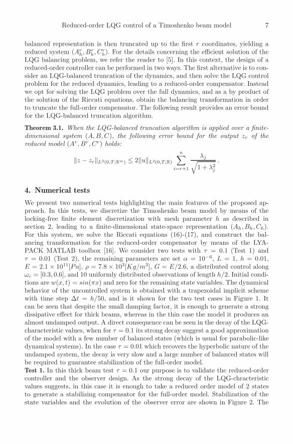
LQG balancing problem, we refer the reader to [5]. In this context, the design of areduced-order controller can be performed in two ways. The first alternative is to con-sider an LQG-balanced truncation of the dynamics, and then solve the LQG controlproblem for the reduced dynamics, leading to a reduced-order compensator. Insteadwe opt for solving the LQG problem over the full dynamics, and as a by product ofthe solution of the Riccati equations, obtain the balancing transformation in orderto truncate the full-order compensator. The following result provides an error boundfor the LQG-balanced truncation algorithm.

Theorem 3.1. When the LQG-balanced truncation algorithm is applied over a finite-dimensional system (A,B,C), the following error bound for the output zr of thereduced model (Ar , Br, Cr) holds:

‖z − zr‖L2(0,T ;Rm) ≤ 2‖u‖L2(0,T ;R)

n∑

i=r+1

λj√

1 + λ2j

.

4. Numerical tests

We present two numerical tests highlighting the main features of the proposed ap-proach. In this tests, we discretize the Timoshenko beam model by means of thelocking-free finite element discretization with mesh parameter h as described insection 2, leading to a finite-dimensional state-space representation (Ah, Bh, Ch).For this system, we solve the Riccati equations (16)-(17), and construct the bal-ancing transformation for the reduced-order compensator by means of the LYA-PACK MATLAB toolbox [16]. We consider two tests with τ = 0.1 (Test 1) andτ = 0.01 (Test 2), the remaining parameters are set α = 10−6, L = 1, h = 0.01,E = 2.1 × 1011[Pa], ρ = 7.8 × 103[Kg/m3], G = E/2.6, a distributed control alongωc = [0.3, 0.6], and 10 uniformly distributed observations of length h/2. Initial condi-tions are w(x, t) = sin(πx) and zero for the remaining state variables. The dynamicalbehavior of the uncontrolled system is obtained with a trapezoidal implicit schemewith time step ∆t = h/50, and is it shown for the two test cases in Figure 1. Itcan be seen that despite the small damping factor, it is enough to generate a strongdissipative effect for thick beams, whereas in the thin case the model it produces analmost undamped output. A direct consequence can be seen in the decay of the LQG-characteristic values, when for τ = 0.1 its strong decay suggest a good approximationof the model with a few number of balanced states (which is usual for parabolic-likedynamical systems). In the case τ = 0.01 which recovers the hyperbolic nature of theundamped system, the decay is very slow and a large number of balanced states willbe required to guarantee stabilization of the full-order model.Test 1. In this thick beam test τ = 0.1 our purpose is to validate the reduced-ordercontroller and the observer design. As the strong decay of the LQG-chracteristicvalues suggests, in this case it is enough to take a reduced order model of 2 statesto generate a stabilizing compensator for the full-order model. Stabilization of thestate variables and the evolution of the observer error are shown in Figure 2. The


Balanced states0 20 40 60 80 100 120

LQG-characteristicvalues

10-15

10-10

10-5

100

105

τ=0.1

τ=0.01

Figure 1. Uncontrolled state w for thickness τ = 0.1 (left) and τ =0.01 (right). The decay of the LQG-characteristic values (middle)provides a guideline for dimensional reduction.

difference between the stabilization rate of the state variables and the decay of theobserver error is due to the scaling of the velocity variables w and θ.

t0 0.1 0.2 0.3 0.4

||y-p

|| [L2 (Ω

)]4

10-6

10-4

10-2

100

102

104

||y-p||[L

2(Ω)]

4

||y-p2||

[L2(Ω)]

4

Figure 2. Test 1. Evolution of the controlled states w (left) and θ(middle) with a reduced-order control of dimension 2. In the right,we see the evolution of the observer error for the full-order estimatep and the reduced-order observer pr.

Test 2. In the thin beam case τ = 0.01, we study the limitations of the proposed ap-proach. As it has been observed in Figure 1, the damping effect in this case is negligi-ble and the low dissipation translates into a very slow decay of the LQG-characteristicvalues. In fact, for less than 20 reduced states, the reduced-order compensator is notable to consistently stabilize the full-order dynamics. The first satisfactory resultsare obtained with r = 22 as shown in Figure 3. Although this is a radically differentscenario if compared with Test 1, it must be noted that the reduced order controllerfor r = 20 has an efficiency factor of 20× with respect to the the full-order compen-sator. Figure 4 indicates that with r = 40 states, i.e. with an efficiency factor of 10×,it is possible to replicate the full order-dynamics and controller in a very accurateway.

Concluding remarks. We have discussed the application of a reduced-order controlalgorithm for the stabilization of the Timoshenko beam model. As a by product of thedesign of an LQG controller, is it possible to obtain a balancing transformation forthe dimensional reduction of the dynamic compensator. In this context, a generic re-quirement for the approach to be successful is the fast decay of the LQG-characteristic


0 0.1 0.2 0.3 0.4−100

−50

0

50

100

t

u

Figure 3. Test 2. Full order controlled w (left), reduced-order (r =22) controlled w (middle) and control signal u(t) (left).

t0 0.1 0.2 0.3 0.4

||y-y

r|| [L2 (Ω

)]4

10-6

10-4

10-2

100

102

104

||y-y22

||[L

2(Ω)]

4

||y-y40

||[L

2(Ω)]

4

t0 0.1 0.2 0.3 0.4

||y-p

|| [L2 (Ω

)]4

10-5

100

105

||y-p||[L

2(Ω)]

4

||y-p22

||[L

2(Ω)]

4

||y-p40

||[L

2(Ω)]

4

Figure 4. Test 2. Evolution of the difference between the statewith full-order control y and the state with reduced-order control yr(left). Difference between the full-order controlled state y and thereduced-order state estimator pr extended to the full space (right).

values. For systems governed by partial differential equations, this relates to the exis-tence of dissipative effects within the system. Therefore in our case the possibility ofsynthesizing a low-complexity controller is conditioned to the interplay between thestructural damping term and the model parameters such as the thickness of the beam.A relevant question that remains open is to determine a lower bound for the numberof reduced states which are necessary for a reduced compensator to guarantee thestabilization of the full-order dynamics. This relates to the H∞ control and reductionproblem. In [15], the authors present a sufficiency test for determining the number ofreduced states for full-order stabilization. However, in our experience these estimatesare not optimal, and therefore we aim at improving the aforementioned bounds forspecific models arising in structural vibration.

Acknowledgments. The authors wish to thank Lars Grune for fruitful discussionswhich motivated this work. The second author was supported by FONDECYT un-der Grant No. 1140392, BASAL Project (CMM, UChile), and CONICYT AnilloACT1106.


References

[1] A. Alla, M. Falcone and D. Kalise. An efficient policy iteration algorithm for dynamicprogramming equations, SIAM J. Sci. Comput., 37(1), 181-200, 2015.

[2] D.N. Arnold. Discretization by finite element of a model dependent parameter problem,Numer. Math. 37 (1981), 405–421.

[3] H.T. Banks and K. Kunisch. The linear regulator problem for parabolic systems, SIAMJ. Control Optim. 22(5) (1984), 684-698.

[4] P. Benner. Solving large-scale control problems, IEEE Control Syst. Mag. 14(1) (2004),44–59.

[5] P. Benner. Balancing-Related Model Reduction for Parabolic Control Systems, Controlof Systems Governed by Partial Differential Equations, IFAC, Volume 1, Part 1, 257–262, 2013.

[6] T. Breiten and K. Kunisch. Compensator design for the monodomain equations,preprint, http://math.uni-graz.at/kunisch/papers/KK_284.pdf.

[7] S. Gugercin and A. Antoulas. A survey of model reduction by balanced truncation andsome new results, Int. J. Control 77(8) (2004), 748–766.

[8] D. Kalise and A. Kroner. Reduced-order minimum time control of advection-reaction-diffusion systems via dynamic programming, Proceedings of the 21st International Sym-posium on Mathematical Theory of Networks and Systems, 1196-1202 (2014).

[9] E. Hernandez, D. Kalise and E. Otarola. A locking-free scheme for the LQR control ofa Timoshenko beam, J. Comput. Appl. Math. 235(5)(2011), 1383–1393.

[10] E. Hernandez and E. Otarola. A locking-free FEM in active vibration control of a Tim-oshenko beam, SIAM J. Numer. Anal. 47 (2009), 2432–2454.

[11] R.E. Kalman. Contributions to the theory of optimal control, Bol. Soc. Mat. Mex. 5(1960), 102–119.

[12] K. Kunisch, S. Volkwein, L. Xie. HJB-POD Based Feedback Design for the OptimalControl of Evolution Problems, SIAM J. on Applied Dynamical Systems 4 (2004), 701-722.

[13] I. Lasiecka and R. Triggiani. Control theory for partial differential equations: continuousand approximations theories, Encyclopedia of mathematics and its applications 74,Cambridge University Press, 2000.

[14] K.A. Morris. Design of finite-dimensional controllers for infinite-dimensional systemsby approximation, J. Math. Systems Estim. Control 6(2)(1996), 151-180.

[15] D. Mustafa and K. Glover. Controller reduction by H-infinity-balanced truncation, IEEETrans. Automat. Control 36(6) (1991), 668-682.

[16] T. Penzl. LYAPACK - Users’ Guide (Version 1.0), available at: ftp://164.41.45.3/pub/netlib/lyapack/guide.pdf.

[17] A. Preumont. Vibration Control of Active Structures, 3rd ed., Solid Mechanics and itsApplications 179, Springer, 2011.

[18] M. Tadi. Optimal infinite-dimensional estimator and compensator for a TimoshenkoBeam, Computers Math. Applic. 27(6) (1994), 19–32.

[19] M. Tadi. Computational algorithm for controlling a Timoshenko beam, Comput. Meth-ods Appl. Mech. Engrg. 153 (1998), 153–165.


Philipp BraunUniversity of BayreuthChair of Applied MathematicsUniversitatsstraße 3095440 Bayreuth, Germanye-mail: [email protected]

Erwin HernandezTechnical University Federico Santa MarıaDepartment of MathematicsAvenida Espana 1680Valparaıso, Chilee-mail: [email protected]

Dante KaliseRadon Institute for Computational and Applied Mathematics (RICAM)Austrian Academy of SciencesAltenbergerstraße 69A-4040 Linz, Austriae-mail: [email protected]

Reduced-order LQG control of a Timoshenko beam model · present numerical tests assessing the stability and performance of ... The theory of optimal feedback control ... Reduced-order

Documents