Redshifts and Killing vectors

arX

iv:g

r-qc

/050

8125

v1 3

1 A

ug 2

005

REDSHIFTS and KILLING VECTORS

Alex Harveya)b)

Visiting ScholarNew York UniversityNew York, NY 10003

Engelbert Schuckingc)

Physics DepartmentNew York University4 Washington PlaceNew York, NY 10003

Eugene J. Surowitzd)

Visiting ScholarNew York UniversityNew York, NY 10003

Abstract

Courses in introductory special and general relativity have increasingly be-come part of the curriculum for upper-level undergraduate physics majors andmaster’s degree candidates. One of the topics rarely discussed is symmetry,particularly in the theory of general relativity. The principal tool for its studyis the Killing vector. We provide an elementary introduction to the concept ofa Killing vector field, its properties, and as an example of its utility apply theseideas to the rigorous determination of gravitational and cosmological redshifts.

1

http://arXiv.org/abs/gr-qc/0508125v1

1 Prologue

In 1907, Albert Einstein enunciated his “equivalence principle” and used it to examinethe influence of the gravitational field on the propagation of light1. He demonstrated,in approximation that as light moved through a difference in gravitational potentialits frequency would change. It is with the latter that the concept of gravitationalredshift enters the ken of the physicist.

In 1916 Einstein completed his journey to a theory of gravitation: The Foun-dations of the General Theory of Relativity2. Here, redshift is studied with greaterprecision. It is discussed in terms of the metric. In Section 22, Behavior of Rods andClocks in the Static Gravitational Field, toward the end of the paper he states, (intranslation) “From this it follows that the spectral lines of light reaching us from thesurface of large stars must appear displaced toward the red end of the spectrum.”

The General Theory of Relativity describes gravitation as the curvature of space-time. The Einstein equations are a protocol for the determination, subject to hypothe-ses concerning the physical nature of the spacetime being discussed, of the metric ofthe space in question. This metric is the source of all information about the proper-ties of the space. In particular, of special interest here, it enables the calculation ofthe paths of light rays—the null geodesics—and the description of the world lines ofobjects in the spacetime.

These ideas were substantially refined and put into the form in use today bythe distinguished mathematician Hermann Weyl. He introduced the concept of worldlines of emitter and observer and the connection of elements of proper time on eachdefined by null geodesics propagating from the former to the latter. This, for the firsttime, provided a general definition of frequency shift for light in arbitrary spacetimes.It was first stated in the fifth edition of his book Space-Time-Matter3. In AppendixIII “Redshift and Cosmology” he explains:

“The different points on the world line of a point-like light source arethe origin of (three-dimensional) surfaces of constant phase that formnull cones opening towards the future. From the rhythm of the changeof phase on this line one obtains the perceived change of phase for anyobserver by checking how his world line intersects the successive surfacesof constant phase. Let s be the proper time of the light source and s′

the proper time of the observer. To each point s on the world line ofthe light source corresponds a point s′ on the world line of the observer:s′ = s′(s), the intersection of his world line with the future null coneemanating from s. If the process occurring at the position of the source is

2

a purely periodic one of infinitely small period then the change of phaseexperienced by the observer is also periodic; but the period is increasedin the ratio 1 + z = ds′/ds (obviously measured along both world linesin their respective proper times). If the observer carries a light sourceof the same physical nature as the observed one then every spectral lineof his light source with frequency f corresponds to the spectral line ofthe distant light source with frequency f/(1 + z). The ones appear to bedisplaced with respect to the others.”

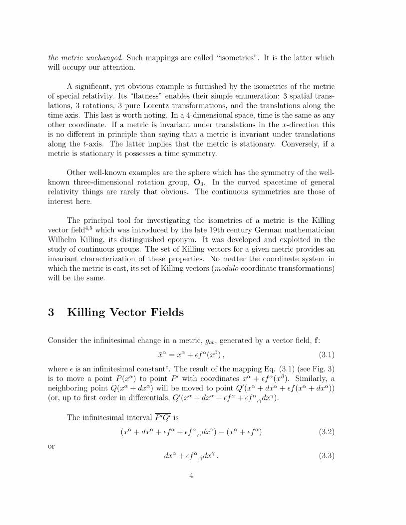
In the ray approximation, light source and observer are connected by nullgeodesics running on surfaces of constant phase of the future light cones. (See Fig. 1).Null geodesics emitted at proper times s and s + ds will intersect the world line ofthe observer at proper times s′ and s′ + ds′ respectively. (See Fig. 2). The redshift issimply

1 + z =ds′

ds. (1.1)

In order to find this ratio one must know the null geodesics, or more precisely, theirvariation. In general this is not simple. The task is greatly simplified if, under a timetranslation, the geodesic is not changed or is subjected only to a scale transformation.These are the conditions, respectively, for the existence of either a Killing vector ora conformal Killing vector in the spacetime manifold. This is the central point of ourinvestigation.

2 Introduction

The concept of symmetry is central to the solution of many problems in physics.Introduction of ignorable coordinates in the construction of kernel functions for La-grangians entails implicit use of a priori knowledge of the symmetries of the systembeing studied. Construction of the Hamiltonian for a problem in quantum mechanicsis constrained by the symmetries thereof. It is the measure of the power of symmetryconsiderations that solely through their application, the Robertson-Walker metric canbe constructed. In this paper we study redshift and, as we shall show, the symmetriesof the spacetime determine the manner in which redshifts occur.

Spacetime is a 4-dimensional Riemannian manifold, that is, it is a surface. Thesymmetries of a surface are numerous: among these there are discrete symmetriessuch as inversion in a point or reflections in a plane and there are the infinitesimalcontinuous coordinate transformations (also called mappings or motions) which leave

3

the metric unchanged. Such mappings are called “isometries”. It is the latter whichwill occupy our attention.

A significant, yet obvious example is furnished by the isometries of the metricof special relativity. Its “flatness” enables their simple enumeration: 3 spatial trans-lations, 3 rotations, 3 pure Lorentz transformations, and the translations along thetime axis. This last is worth noting. In a 4-dimensional space, time is the same as anyother coordinate. If a metric is invariant under translations in the x-direction thisis no different in principle than saying that a metric is invariant under translationsalong the t-axis. The latter implies that the metric is stationary. Conversely, if ametric is stationary it possesses a time symmetry.

Other well-known examples are the sphere which has the symmetry of the well-known three-dimensional rotation group, O3. In the curved spacetime of generalrelativity things are rarely that obvious. The continuous symmetries are those ofinterest here.

The principal tool for investigating the isometries of a metric is the Killingvector field4,5 which was introduced by the late 19th century German mathematicianWilhelm Killing, its distinguished eponym. It was developed and exploited in thestudy of continuous groups. The set of Killing vectors for a given metric provides aninvariant characterization of these properties. No matter the coordinate system inwhich the metric is cast, its set of Killing vectors (modulo coordinate transformations)will be the same.

3 Killing Vector Fields

Consider the infinitesimal change in a metric, gab, generated by a vector field, f :

xα = xα + ǫfα(xβ) , (3.1)

where ǫ is an infinitesimal constante. The result of the mapping Eq. (3.1) (see Fig. 3)is to move a point P (xα) to point P ′ with coordinates xα + ǫfα(xβ). Similarly, aneighboring point Q(xα + dxα) will be moved to point Q′(xα + dxα + ǫf(xα + dxα))(or, up to first order in differentials, Q′(xα + dxα + ǫfα + ǫfα

,γdxγ).

The infinitesimal interval P ′Q′ is

(xα + dxα + ǫfα + ǫfα,γdxγ) − (xα + ǫfα) (3.2)

ordxα + ǫfα

,γdxγ . (3.3)

4

The length, ds2, of this interval is given by

ds2

= gαβ(xγ + ǫf γ)(dxα + ǫfα,κdxκ)(dxβ + ǫfβ

,κdxκ)

= (gαβ + ǫgαβ,γfγ)(dxα + ǫfα

,γdxγ)(dxβ + ǫfβ,κdxκ) . (3.4)

Expanding Eq. (3.4), neglecting terms of order ǫ2, and rearranging dummy indicesresults in

ds2

= gαβdxαdxβ + ǫ(gαβ,γfγ + gαγf

γ,β + gγβfγ

,α)dxαdxβ . (3.5)

With the definition2sαβ ≡ gαβ,γf

γ + gαγfγ,β + gγβfγ

,α (3.6)

the change in the metric may be written as

1

ǫ(ds

2 − ds2) = 2sαβdxα dxβ . (3.7)

Because the left hand side of this equation is a scalar and dxα dxβ is a symmetrictensor it may be inferred that the symmetric quantity sαβ is a covariant tensor6.

The structure of the right hand side of Eq. (3.6)

gαβ,γfγ + gαγf

γ,β + gγβfγ

,α (3.8)

combines partial differentiation and a vector field and arises in precisely this formin many applications. The operation is important enough to have its own name andsymbol. It is called the “Lie derivative” of a geometric object (in this instance, themetric tensor, gab) with respect to a vector field, f , and is written Lf . Thus, Eq.(3.6) may be written as

Lfgαβ = 2sαβ . (3.9)

In the special case where the metric tensor is invariant under the transformationwe will have Lfgαβ = 0. Then the vector f is, by definition, a Killing vector. Killingvectors are customarily designated by the symbol ξ. For Killing vectors, then, wehave

Lξgαβ = gαβ,γξγ + gαγξ

γ,β + gβγξ

γ,α = 0 . (3.10)

This equation can be written in a different form, useful for many purposes, viz.,

Lξgαβ = ξα;β + ξβ;α = 0 . (3.11)

The identity of these 2 forms can be demonstrated by expressing both in geodeticcoordinates. The result is identical expressions. Consequently, they are identicalin any choice of coordinates. Alternatively, expansion of the covariant derivativesof Eq. (3.11) yields precisely Eq. (3.10). Any 2-index tensor may be expressed as

5

the sum of a symmetric and skew-symmetric tensor. Equation (3.11) indicates thatthe symmetric part of the tensor ξα;β vanishes. Because infinitesimal displacementsgenerated by Killing vectors leave the metric unchanged, these displacements mapgeodesics onto neighboring geodesics. Note, also, that Eqs. (3.6) may be read ineither of two ways. Given a metric, they provide the means for the determination ofits Killing vectors or given a set of Killing vectors, determining the metric. The latteris ill-defined.

4 Killing Vectors in Flat Spacetimes

In flat spacetimes Cartesian coordinates may be introduced. Consequently, in Eqs.(3.11), covariant derivatives may be replaced by partial derivatives and the right handportion becomes

ξα,β + ξβ,α = 0 . (4.1)

By differentiation we getξα,β,γ + ξβ,α,γ = 0 (4.2)

and by cyclic permutation of the indices we obtain

ξβ,γ,α + ξγ,β,α = 0 (4.3)

andξγ,α,β + ξα,γ,β = 0 . (4.4)

Addition of Eqs. (4.2) and (4.3), subtraction of Eq. (4.4), and recognition that secondpartial derivatives commute, results in the differential equations

2ξγ,α,β = 0 . (4.5)

The solutions of these equations are the general linear functions

ξα = Aαβxβ + Bα (4.6)

where Aαβ and Bα are constants. If Eq. (4.6) is substituted into Eq. (4.1) we findimmediately that Aαβ is skew-symmetric

Aαβ = −Aβα . (4.7)

We see, thus, that an n-dimensional flat space has n(n + 1)/2 independent Killingvectors. For Minkowski spacetime this is just 10. This demonstration depends inan essential way on the flatness of the spacetime. It is this fact which permits thesubstitution of partial for covariant differentiation and consequent ability to reorderthe differentiation.

6

5 Conformal and Homothetic Motions

In addition to the mappings described by Killing vectors, there are other classesof transformations generated by vector fields which are important in the presentcontext. These are the so called “homothetic” and “conformal” motions. In thesecases, respectively, the metric tensor is either multiplied by a constant or a scalarfunction. The generators are termed homothetic or conformal Killing vectors. Inthese cases the stress tensor is proportional to the metric. Both cases are subsumedin

ξα;β + ξβ;α = gαβ,γξγ + gαγξ

γ,β + gγβξγ

,α = 2σgαβ . (5.1)

It is simple to determine σ. Contract Eq. (5.1) with gαβ; simple manipulationyields σ = ξγ

;γ/n and

gαβ,γξγ + gαγξ

γ,β + gγβξγ

,α =2

nξγ

;γgαβ (5.2)

where n is the dimension of the manifold. If ξγ;γ is a constant, the Killing vector, by

definition, describes homothetic motions; and if ξγ;γ is a scalar field, say φ(xα), the

motion is called conformal.

Similarly to Eqs. (3.11) this may be written as

ξα;β + ξβ;α =2

nξγ

;γgαβ or

Lξgαβ =2

nξγ

;γgαβ (5.3)

In this instance the trace-free symmetric part of ξα;β vanishes.

Again, for flat spacetimes, the situation is vastly simplified. A special homoth-etic Killing vector is given by

ξα = κxα (5.4)

where κ is a constant. (See Fig. 4.) The most general homothetic Killing vector is

ξα = (κηαβ + Aαβ)xβ + Bα (5.5)

where Aαβ = −Aβα. This is readily verified by substitution into in Eq. (5.1) andreplacing covariant by partial derivatives. In this instance the coordinate grid isuniformly stretched or shrunk. Similarly, it is easy to confirm that

ξα = (ηαβCγ −1

2ηβγCα)xβxγ (5.6)

where ηαβ is the flat space metric and Cγ are constants, are special conformal Killingvectors.

7

6 Redshifts Derived from Killing Vectors

The calculation of redshifts is extremely simple in spacetimes possessed of time-likeconformal Killing vector fields parallel to the world lines of source and observer.Consider Eq. (1.1), Weyl’s universal definition of redshift,

1 + z =ds′

ds. (6.1)

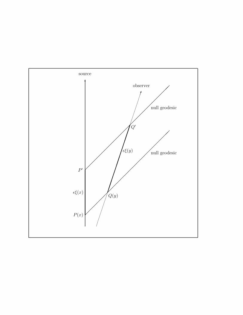
The event P (xα) at the source is connected to the event Q(yα) at the observer bya null geodesic. (See Fig 4.) A conformal Killing vector field ξa moves P (xα) intoP ′(xα + ǫξa(xβ))and Q(yα) into Q′(yα + ǫξa(yβ)) and the null geodesic connecting Pand Q into the null geodesic connecting P ′ and Q′. We have then respectively

ds =| ǫξa(xβ) | and ds′ =| ǫξα(yβ) | (6.2)

and thus

1 + z =

√

√

√

√

gαβ(yγ)ξα(yγ)ξβ(yγ)

gαβ(xγ)ξα(xγ)ξβ(xγ). (6.3)

This holds if the Killing vector field is tangent to the world line of the source at itspoint of emission and tangent to the observer’s world line at the point of reception. Ifsource and observer move on conformal time-like Killing lines this condition is fulfilledat all times.

7 Doppler Effect in Minkowski Spacetime

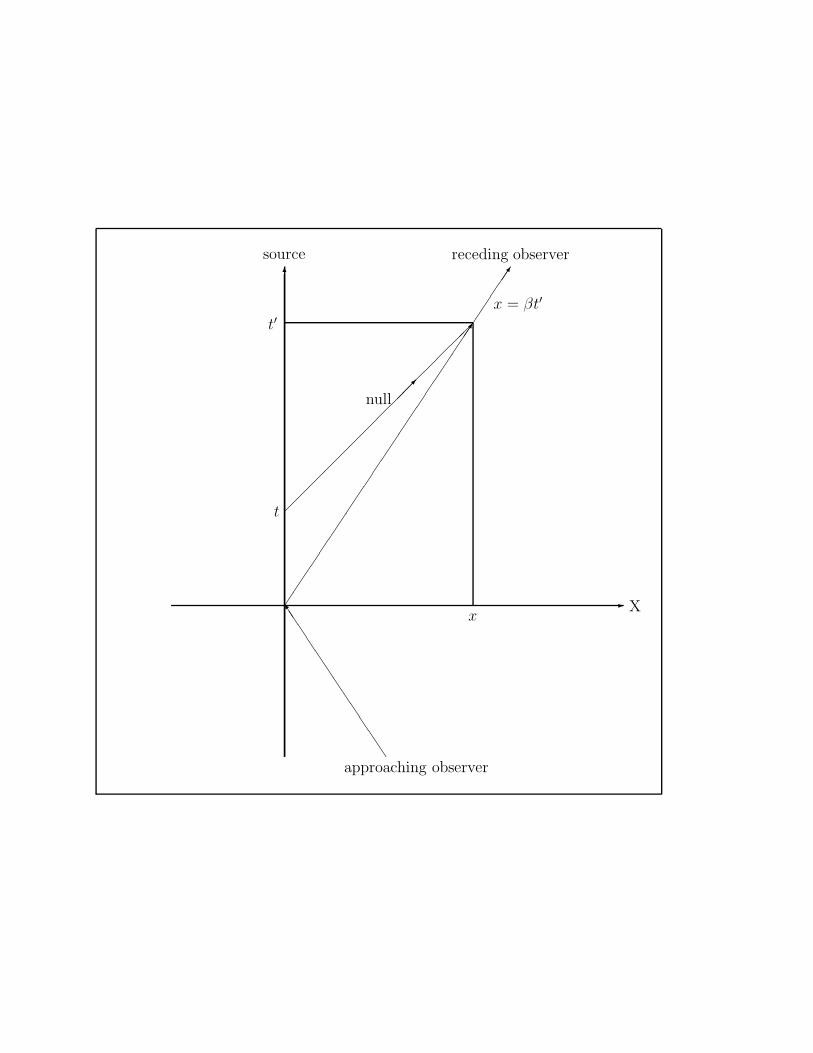
Weyl’s definition of redshift, 1 + z = ds′/ds, readily provides the usual formula forrelativistic Doppler effect in flat spacetime. Take the world line of the source to be

x0 = tx = y = z = 0 .

(7.1)

For the world line of the (inertial) observer we take a straight line through theorigin with slope β

x = βt, y = z = 0 . (7.2)

Light emitted by the source at time t will be received by the observer at time t′. (SeeFig. 5.) If the observer is receding from the source he or she will see the light at

x′ = βt′ y′ = z′ = 0 . (7.3)

8

The homothetic Killing vector (5.4) has the lengths, respectively, at source and ob-server of κt and κ(t

′2 − x′2)1/2. We readily obtain from Eq. (6.3)

1 + z =

√

√

√

√

gαβ(yγ)ξα(yγ)ξβ(yγ)

gαβ(xγ)ξα(xγ)ξβ(xγ)

=

√t′2 − x′2

t

=t′√

1 − β2

t′ − x′

=

√1 − β2

1 − β

=

√

1 + β

1 − β(7.4)

This is the relativistic Doppler formula for a receding observer. For an approachingobserver replace β by −β.

It is instructive to apply Weyl’s definition of redshift, Eq. (1.1) to Minkowskispacetime with the spatial part expressed in polar spherical coordinates.

ds2 = dt2 − dr2 − r2(dθ2 + sin2 θ dφ2) . (7.5)

We introduce 4-dimensional polar coordinates with the coordinate transformation(

tr

)

=

(

T cosh χT sinh χ

)

. (7.6)

The differentials are

dt = dT cosh χ + T sinh χdχ

dr = dT sinh χ + T cosh χdχ (7.7)

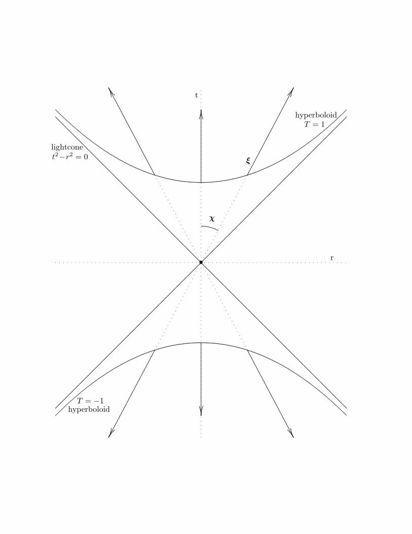
The result isds2 = dT 2 − T 2 [dχ2 + sinh2 χ (dθ2 + sin2 θ dφ2)] . (7.8)

This maps the interiors of the past and future light-cones of Minkowski spacetimeinto, respectively, linearly contracting and expanding spaces of constant negativecurvature. (See Fig. 6.) A straight world line through the origin would be just

β =r

t(7.9)

which by virtue of Eqs. (7.6) would map into

β = tanhχ . (7.10)

9

In the mapped space, such lines are, at constant {χ, θ, φ} with χ as the rapidity.We now use the homothetic Killing vector Eq. (5.4) to construct a linear first-orderdifferential form

ξαdxα = κxαdxα = κ(t dt − r dr) . (7.11)

In Eq. (7.8), with use of Eqs.(7.7), this is readily found to be

ξαdxα = κTdT . (7.12)

The length of the homothetic killing vector in the new coordinate system is thus κTand the redshift is

1 + z =T ′

T. (7.13)

8 More Redshifts

8.1 Cosmological Redshifts

The last example leads us directly to the calculation of redshift in the Friedmanncosmological models7,8

ds2 = dt2 − R2(t)[dχ2 + S2(χ)(dθ2 + sin2 θdφ2)] (8.1)

where S determines the curvature of the 3-space,

S =

sin χ , positiveχ , flat

sinh χ , negative

. (8.2)

With Eq. (5.2)


γ,β + gγβξγ

,α =2

nξγ

;γgαβ (8.3)

it is readily confirmed thatξα = R(t)δα

0 (8.4)

is a conformal Killing vector tangent to the world line of the source at χ = 0 and alsotangent to the observer’s world line at {χ, θ, φ = constant}.

It follows from application of Eq. (6.3) that the redshift is

1 + z =R(t′)

R(t)(8.5)

for a light signal emitted at time t and received at t′.

10

8.2 Redshifts in Stationary Spacetimes

The general stationary spacetime may be written as

ds2 = goodt2 + 2goidtdxi + gijdxidxj (8.6)

with ∂gαβ/∂t = 0.

Because the field is stationary it necessarily possesses a time-like Killing vector.The simplest assumption is

ξα = δα0 . (8.7)

This is readily verified by use of Eq. (3.10)


γ,β + gβγξ

γ,α = 0 . (8.8)

We then have, as earlier,

1 + z =

√

√

√

√

gαβ(x′)ξα(x′)ξβ(x′)

gγδ(x)ξγ(x)ξδ(x)

=

√

√

√

√

goo(x′)

goo(x). (8.9)

If the world line of the source is xj = const and that of the observer is x′j = const,both are tangent to a Killing vector of this field.

One of the most important of the stationary metrics is the Schwarzschild-Droste(SD) metric It is scarcely known among relativists that the determination of the metricfor a point mass was accomplished almost simultaneously with Karl Schwarzschild byJohannes Droste, a Ph.D. student of H. A. Lorentz. The form of the metric (8.10)was actually due to Droste9.

ds2 =(

1 − 2m

r

)

dt2 −(

1 − 2m

r

)−1

dr2 − r2(dθ2 + sin2 θdφ2) . (8.10)

By virtue of the Birkhoff theorem10,11, all spherically symmetric, vacuum metrics arestationary and equivalent to Eq. (8.10). Application of Eq. (8.9) yields the redshift

1 + z =

√

√

√

√

1 − 2m/r′

1 − 2m/r. (8.11)

For the case where r′ = r + δr with δr << r we easily obtain

11

z =δν

ν= −G M δr

c2 r2. (8.12)

In the usual special relativistic approximation12 the “mass” of the photon istaken to be hν/c2 and the change in energy as it moves through a vertical distanceδr is

∆E =hν

c2g δr (8.13)

where g is the local gravitational acceleration GM/r2.

8.3 Comments

Both the preceeding subsections discuss “elementary” situations. In the cosmologicalcase the emitter is at rest in the coordinate system given by the metric (8.6). Inphysical terms terms it is at rest with respect to the background microwave radiationor equivalently, has no “peculiar” motion. If the emitter does have a peculiar velocitythe situation is substantially more complicated. Moreover the usual observers areeither earthbound astronomers or the Hubble Telescope which provides a peculiarmotion at the receiving end. But, this is quite small relative to other sources of error.

In the case of redshift due to differences in gravitational potential of emitter andobserver in a stationary spacetime the situation is more clearly defined. An exampleis the Pound-Rebka experiment13 where the difference is precisely known and bothemitter and observer are at rest. A different and substantially more complex situationis is presented by the Global Positioning System14. Here, the observers are at restand the emitters are not only at a different gravitational potential, they are movingwith high velocity If a metric has Killing vectors in addition to the ones discussedfor the radial Doppler effects they can be used for describing Doppler effect due torelative velocities of sources and observers with respect to a distinguished time-likedirection given by a (conformal) Killing vector defining a local state of rest.

9 Conservation Theorems

One of the most important properties of Killing vectors is their utility in the derivationof conservation theorems. These are obtained in conjuction with the tangent vectorsof geodesics. These are the null vectors for photons and the tangent vectors for

12

force-free point masses. The geodesics are provided by the solutions of the geodesicequation

dkα

dλ+

{

αβ γ

}

kβkγ = 0 (9.1)

where λ is an affine parameter 15 along the trajectory and kα = dxα/dλ. Note thatEq. (9.1) may be written as

kα;βkβ = 0 . (9.2)

Also, for photons and unit masses we have, respectively

kαkα = 0 and 1 . (9.3)

For a Killing vector, ξ and the tangent vector, k, to a geodesic, the product E = ξαkα

is constant along the geodesic. This product is constant because the directionalderivative of E along the geodesic vanishes.

E ≡ (kαξα);βkβ

= kα;βkβξα + ξα;βk

αkβ = 0 . (9.4)

On the right hand side the first and second terms vanish by virtue, respectively, ofthe geodesic equation, Eq. (9.2) and the skew-symmetry of ξα;β. (See Eq. (3.11).)Consequently, E = 0 and E is constant along the geodesic.

Equation (9.4) is valid for either photons or point masses. For photons there isan additional possibility. If the metric admits either a homothetic or conformal Killingvector a similar integral exists. The second term in Eq. (9.4) will vanish because ξα;β issymmetric and proportional to gαβ and kα is a null vector. In either event the integralis identical in form to that for Killing vector fields, that is, E = ξα kα = constant.

Killing vectors are indispensable for the invariant formulation of conservationtheorems for fields and extended bodies. Local conservation laws are expressed as thecovariant divergence of a symmetric tensor

T αβ;β = 0 , T αβ = T βα . (9.5)

Given a Killing vector ξα define the quantity Sβ ≡ ξaTαβ. We then have

Sβ;β = ξα;βT

αβ + ξαT αβ;β = 0 . (9.6)

The first term vanishes because skew-symmetric and symmetric tensors are con-tracted; the second term vanishes by virtue of the definition of one of its factors.Now, the covariant divergence of a vector may be written as16

Sβ;β =

1√−g(√−gSβ),β = 0 . (9.7)

13

which is a true conservation law.

If, in addition to being symmetric, T αβ has a vanishing trace, that is T αβgαβ = 0,as is the important case of electromagnetic energy-momentum tensor, then conserva-tion laws involving conformal Killing vectors may be obtained. In the first term ofEq. (9.6) substitute in accordance Eq. (5.1). This results immediately in

Sβ;β = σgαβT αβ + ξαT αβ

;β = 0 . (9.8)

On the right hand side both terms obviously vanish.

a)Professor Emeritus, Queens College, City University of New York

Electronic mail: [email protected]@[email protected]

eThe following conventions are used: c = 1 with metric signature [1, −1, −1, −1]; co-ordinate indices range from [0−3] and in arbitrary coordinate systems are designatedby lower case Greek letters, i.e., [α, β, γ, . . . ]; spatial indices range from [1− 3] andare designated by lower case Roman case letters [i, k, j, . . . ]; in Cartesian coordinatesystems we use [t, x, y, z]; partial and covariant differentiation are indicated, respec-

tively, by commas or semicolons, viz., fα,β = ∂fα

∂xβ and fα;β = ∂fα

∂xβ +

{

αβ γ

}

fγ.

1A. Einstein, “Uber das Relativitats Prinzip und die aus demselben gezogenen Fol-gerungen” [On the Relativity Principle and the Conclusions drawn from it], Jahrbuchder Radioaktivitat und Elektronik , 4, pp. 411–462 (1907). An English translation isavailable in vol.2, “Collected Papers of Albert Einstein”, translator A. Beck, consul-tant P. Havas, Princeton University Press, Princeton, NJ, (1989) pp. 252–311.

2A. Einstein, “ Die Grundlage der allgemeinen Relativitatstheorie, Annalen der Physik ,49, pp. 769–822 (1916). An English translation is contained in vol. 6 “Collected Pa-pers of Albert Einstein”, translator A. Engel, consultant E. L. Schucking, PrincetonUniversity Press, Princeton, NJ, (1997) pp. 147–200.

3H. Weyl, Raum-Zeit-Materie, 5th edition, Springer-Verlag, Berlin (1923). This wasedited and annotated by Juergen Ehlers and reprinted as the 7th edition, Springer-Verlag, Berlin (1988). The English translation is by E. L. Schucking.

4See, e.g., R. d’Inverno, Introducing Einstein’s Relativity, Clarendon Press, Oxford(1992), Section 7.7.

5S. W. Carroll, Spacetime and Geometry, Addison Wesley, New York (2004). Seesection 3.8.

14

6In 3-dimensional elasticity theory this tensor is known as the strain tensor due to aninfinitesimal displacement ǫf i(xj). See, e.g., F. Ziegler, Mechanics of Solids and Flu-ids, Springer-Verlag, New York (1991). See section 1.3, “Kinematics of DeformableBodies”.

7W. Rindler, Relativity - Special, General, Cosmological , Oxford University Press,New York (2001). See sections 16.4 and 16.5.

8S. W. Carroll, loc cit, section 8.2.

9A note by T. Rothman discussing its genesis and content has appeared as a “GoldenOldie” in General Relativity and Gravitation, 34, pp.1541–1543 (2002).

10R. d’Inverno, loc cit, section 14.6.

11S. W. Carroll, loc cit, section 5.2.

12W. Rindler, loc cit, pp. 4–26.

13R. V. Pound and G. A. Rebka, “Apparent Weight of Photons”, Physical ReviewLetters, 4, pp. 337–341 (1960).

14N. Ashby, “Relativity and the Global Positioning System”, Physics Today, May2002 pp. 41-47; “Relativity in the Global Positioning System”, Living Reviews inRelativity, http://www.livingreviews.org/lrr–2003–1, Max-Planck-Gesellschaft, Pots-dam, Germany (2003).

15S. W. Carroll, loc cit, section 3.4

16S. W. Carroll, loc cit, see p. 101.

15

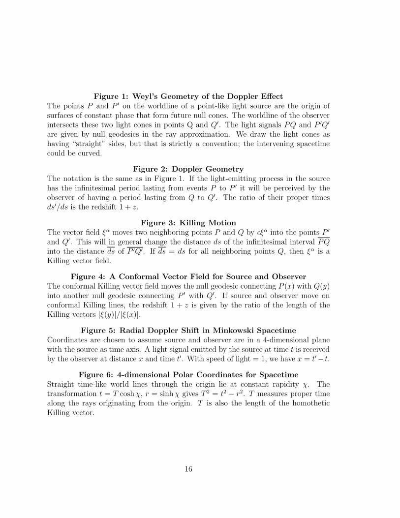
Figure 1: Weyl’s Geometry of the Doppler Effect

The points P and P ′ on the worldline of a point-like light source are the origin ofsurfaces of constant phase that form future null cones. The worldline of the observerintersects these two light cones in points Q and Q′. The light signals PQ and P ′Q′

are given by null geodesics in the ray approximation. We draw the light cones ashaving “straight” sides, but that is strictly a convention; the intervening spacetimecould be curved.

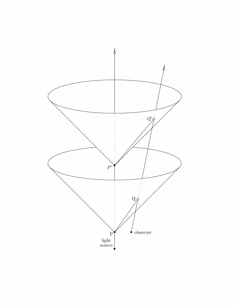
Figure 2: Doppler Geometry

The notation is the same as in Figure 1. If the light-emitting process in the sourcehas the infinitesimal period lasting from events P to P ′ it will be perceived by theobserver of having a period lasting from Q to Q′. The ratio of their proper timesds′/ds is the redshift 1 + z.

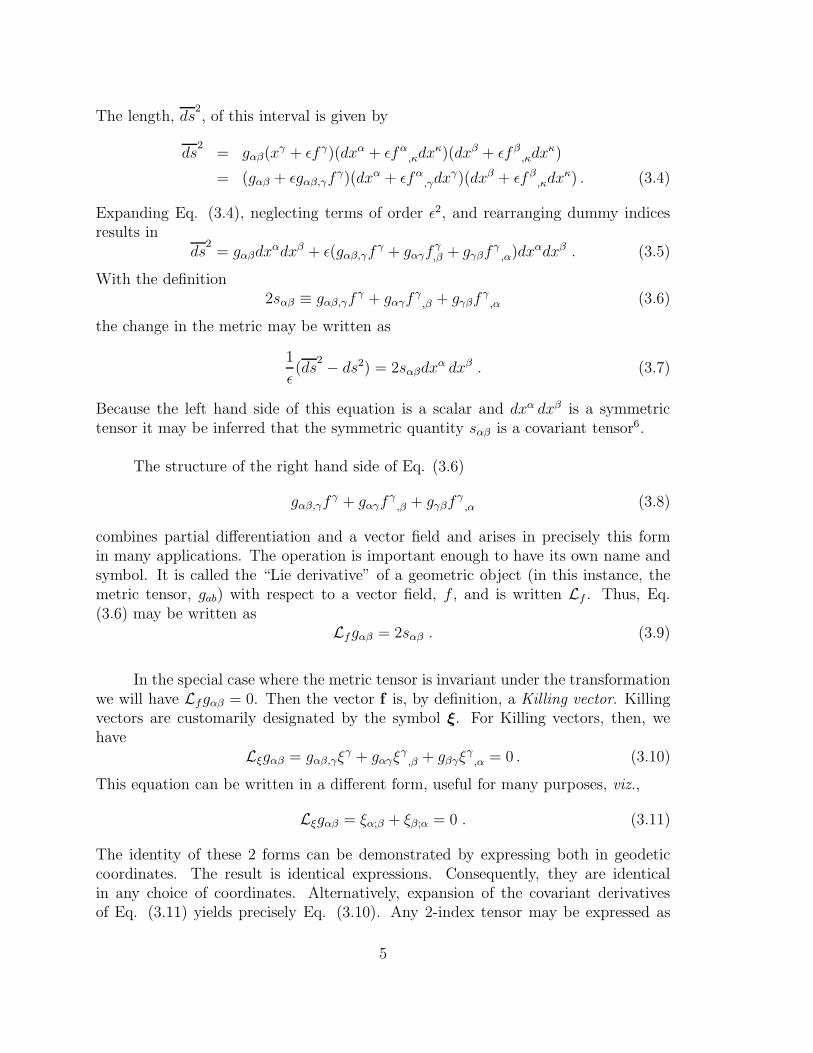
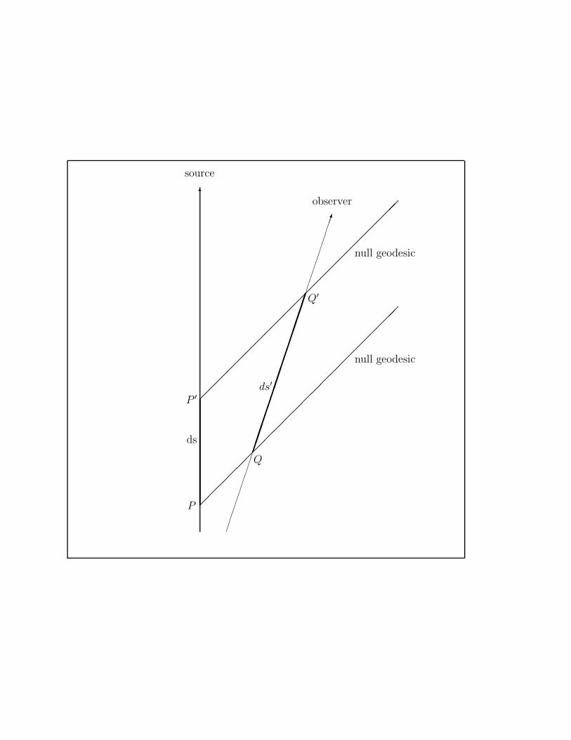
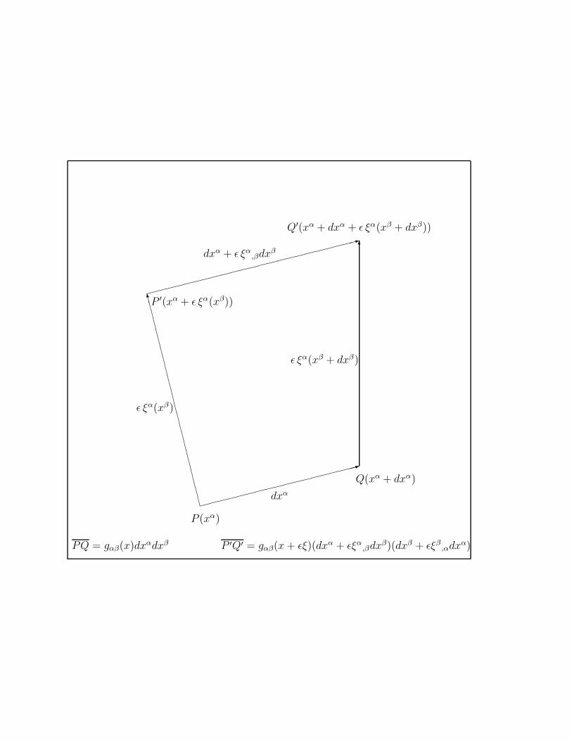
Figure 3: Killing Motion

The vector field ξα moves two neighboring points P and Q by ǫξα into the points P ′

and Q′. This will in general change the distance ds of the infinitesimal interval PQinto the distance ds of P ′Q′. If ds = ds for all neighboring points Q, then ξα is aKilling vector field.

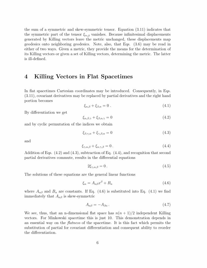
Figure 4: A Conformal Vector Field for Source and Observer

The conformal Killing vector field moves the null geodesic connecting P (x) with Q(y)into another null geodesic connecting P ′ with Q′. If source and observer move onconformal Killing lines, the redshift 1 + z is given by the ratio of the length of theKilling vectors |ξ(y)|/|ξ(x)|.

Figure 5: Radial Doppler Shift in Minkowski Spacetime

Coordinates are chosen to assume source and observer are in a 4-dimensional planewith the source as time axis. A light signal emitted by the source at time t is receivedby the observer at distance x and time t′. With speed of light = 1, we have x = t′− t.

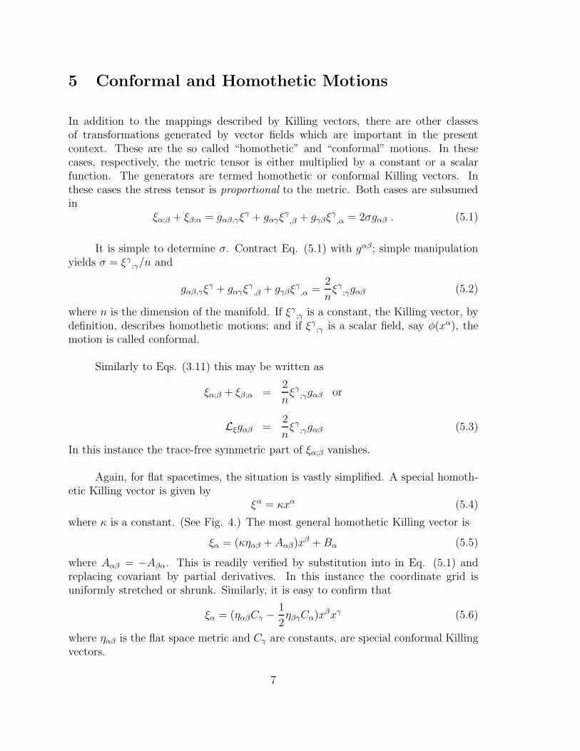
Figure 6: 4-dimensional Polar Coordinates for Spacetime

Straight time-like world lines through the origin lie at constant rapidity χ. Thetransformation t = T cosh χ, r = sinh χ gives T 2 = t2 − r2. T measures proper timealong the rays originating from the origin. T is also the length of the homotheticKilling vector.

16

.

.

.

.

.

.

.

.

.

.

.

..

.

..

.

...............................................................................................................................................................

............

.............

..............

................

..................

.....................

..........................

........................................

...................................................................................................................................................................................................................................................................................................................................................................................................................................................................................................................................................................................................................................................................................................................................................................................................................................................................................................

.............................................

.............................

.................................................................................................................................................................................................................................................................................

.

.

.

.

.

.

..

.

.

.

..

.

.

..

.

..........................................................................................................................................................................................................................................................................................................................................................................................................................

..............................................

............................

......................

..................

................

...............

.............

............

...........

......................................................................................................................................................................

.

.

.

.

.

.

.

.

.

.

.

..

.

..

.

...............................................................................................................................................................

............

.............

..............

................

..................

.....................

..................

.

.

.

.

.

.

.

.

.

.

.

..

.

..

.

..

.

..

....................................................................................................................................................................................................................................................................

......

•

•

• •P

P ′

Q

Q′

lightsource

observer

.

.

.........................................................................................................................................................................................................................................................................................................................................

.

.

..

.

..

..

.

...................................................................................................................................................................................................................

.

.

.

.

.

.

.

.

.

.

.

.

.

.

.

.

.

.

.

.

.

.

.

.

.

.

.

.

.

.

.

.

.

.

.

.

.

.

.

.

.

.

.

.

.

.

.

.

.

.

.

.

.

.

.

.

.

.

.

.

.

.

.

.

.

.

.

.

.

.

.

.

.

.

.

.

.

.

.

.

.

.

.

.

.

.

.

.

.

.

.

.

.

.

.

.

.

.

.

.

.

.

.

.

.

.

.

.

.

.

.

.

.

.

.

.

.

.

.

.

.

.

.

.

.

.

.

.

.

.

.

.

.

.

.

.

.

.

.

.

.

.

.

.

.

.

.

.

.

.

.

.

.

.

.

.

.

.

.

.

.

.

.

.

.

.

.

.

.

.

.

.

.

.

.

.

.

.

.

.

.

.

.

..

.

.

.

.

.

.

.

.

.

.

.

.

.

.

.

.

.

.

.

.

.

.

.

.

.

.

.

.

.

.

.

.

.

.

.

.

.

.

.

.

.

.

.

.

.

.

.

.

.

.

.

.

.

.

.

.

.

.

.

.

.

.

.

.

.

.

.

.

.

.

.

.

.

.

.

.

.

.

.

.

.

.

.

.

.

.

.

.

.

.

.

.

.

.

.

.

.

.

.

.

.

.

.

.

.

.

.

.

.

.

.

.

.

.

.

.

.

.

.

.

.

.

.

.

.

.

.

.

.

.

.

.

.

.

.

.

.

.

.

.

.

.

.

.

.

.

.

.

.

.

.

.

.

.

.

.

.

.

.

.

.

.

.

.

.

.

.

.

.

.

.

.

.

.

.

.

.

.

.

.

.

.

.

.

.

.

.

.

.

.

.

.

.

.

.

.

.

.

.

.

.

.

.

.

.

.

.

.

.

.

.

.

.

.

.

.

.

.

.

.

.

.

.

.

.

.

.

.

.

.

.

.

.

.

.

.

.

.

.

.

.

.

.

.

.

.

.

.

.

.

.

.

.

.

.

.

.

.

.

.

.

.

.

.

.

.

.

.

.

.

.

.

.

.

.

.

.

.

.

.

.

.

.

.

.

.

..

.

.

.

.

.

.

.

.

.

.

.

.

.

.

.

.

.

.

.

.

.

.

.

.

.

.

.

.

.

.

.

.

.

.

.

.

.

.

.

.

.

.

.

.

..

.

.

.

.

.

.

.

.

.

.

..

.

.

.

.

.

.

.

.

.

.

.

.

..

.

.

.

.

.

.

.

.

.

.

.

.

.

.

.

..

.

.

.

.

.

.

.

.

.

.

.

.

..

.

.

.

.

.

..

.

.

.

.

.

.

.

.

.

.

.

.

.

.

.

.

.

.

.

..

.

.

.

.

.

.

.

.

.

.

.

.

.

.

.

.

.

.

.

.

..

.

.

.

.

.

.

.

.

.

.

.

.

.

.

.

.

.

.

.

.

..

.

.

.

.

.

.

.

.

.

.

.

.

.

.

.

.

.

.

.

.

..

.

.

.

.

.

.

.

.

.

.

.

.

.

.

.

.

.

.

.

.

..

.

.

.

.

.

.

.

.

.

.

.

.

.

.

.

.

.

.

.

.

..

.

.

.

.

.

.

.

.

.

.

.

.

.

.

.

.

.

.

.

.

..

.

.

.

.

.

.

.

.

.

.

.

.

.

.

.

.

.

.

.

..

.

.

.

.

.

.

.

.

.

.

.

.

.

.

.

.

.

.

.

.

..

.

.

.

.

.

.

.

.

.

.

.

.

.

.

.

.

.

.

.

.

..

.

.

.

.

.

.

.

.

.

.

.

.

.

.

.

.

.

.

.

.

..

.

.

..

.

.

.

.

.

..

.

.

.

.

.

.

.

.

.

.

.

.

.

.

.

.

.

.

.

.

.

.

.

.

.

.

..

.

.

.

.

.

.

.

.

..

.

.

.

..

.

.

.

..

.

.....

.

.

.

.

.

.

.

.

.

.

.

.

.

.

.

..

.

.

.

.

.

.

.

.

.

.

.

.

.

.

.

.

.

.

.

.

.

.

..

.

.

.

.

.

.

.

.

.

.

.

.

.

.

.

.

.

.

.

.

.

.

..

.

.

.

.

.

.

.

.

.

.

.

.

.

.

.

.

.

.

.

.

.

.

..

.

.

.

.

.

.

.

.

.

.

.

.

.

.

.

.

.

.

.

.

.

.

..

.

.

.

.

.

.

.

.

.

.

.

.

.

.

.

.

.

.

.

.

.

..

.

.

.

.

.

.

.

.

.

.

.

.

.

.

.

.

.

.

.

.

.

.

..

.

.

.

.

.

.

.

.

.

.

.

.

.

.

.

.

.

.

.

.

.

.

..

.

.

.

.

.

.

.

.

.

.

.

.

.

.

.

.

.

.

.

.

.

.

..

.

.

.

.

.

.

.

.

.

.

.

.

.

.

.

.

.

.

.

.

.

.

..

.

.

.

.

.

.

.

.

.

.

.

.

.

.

.

.

.

.

.

.

.

.

..

.

.

.

.

.

.

.

.

.

.

.

.

.

.

.

.

.

.

.

.

.

.

..

.

.

.

.

.

.

.

.

.

.

.

.

.

.

.

.

.

.

.

.

.

.

..

.

.

.

.

.

.

.

.

.

.

.

.

.

.

.

.

.

.

.

.

.

.

..

.

.

.

.

.

.

.

.

.

.

.

.

.

.

.

.

.

.

.

.

.

.

..

.

.

.

.

.

.

.

.

.

.

.

.

.

.

.

.

.

.

.

.

.

..

.

.

.

.

.

.

.

.

.

.

.

.

.

.

.

.

.

.

.

.

.

..

.

.

.

.

.

.

.

.

.

.

.

.

.

.

.

.

.

.

.

.

.

..

.

.

.

.

.

.

.

.

.

.

.

.

.

.

.

.

.

.

.

.

.

..

.

.

.

.

.

.

.

.

.

.

.

.

.

.

.

.

.

.

.

.

.

..

.

.

.

.

.

.

.

.

.

.

.

.

.

.

.

.

.

.

.

.

.

..

.

.

.

.

.

.

.

.

.

.

.

.

.

.

.

.

.

.

.

.

.

..

.

.

.

.

.

.

.

.

.

.

.

.

.

.

.

.

.

.

.

.

.

.

.

.

.

.

.

.

.

.

.

.

.

.

.

.

.

.

.

.

.

.

.

.

.

.

.

.

.

.

.

.

.

.

.

.

.

.

.

.

.

.

.

..

.............................................................................................................................................................................................................................................................................................................................................................................................................................................................................................................

.

...............................................................................................................................................................................................................................................................................................................................................................................................................................................................................................................

.

...............................................................................................................................................................................................................................................................................................................................................................................................................................................................................................................

.

..

.............................................................................................................................................................................................................................................................................................................................................................................................................................................................................................................

⊙

⊙

6

��

��

��

��

��

��

��

��

��

��

��

��

��

��

��

��

��

��

��

��

��

��

��

��

��

��

��

��

��

��

��

��

��

��

��

��

��

��

��

��

��

��

��

��

��

��

��

��

source

observer

P

P ′

Q

Q′

ds

ds′

null geodesic

null geodesic

CCCCCCCCCCCCCCCCCCCCCCCO

��:

6

��:

P (xα)

Q(xα + dxα)

P ′(xα + ǫ ξα(xβ))

Q′(xα + dxα + ǫ ξα(xβ + dxβ))

dxα

ǫ ξα(xβ)

ǫ ξα(xβ + dxβ)

dxα + ǫ ξα,βdxβ

PQ = gαβ(x)dxαdxβ P ′Q′ = gαβ(x + ǫξ)(dxα + ǫξα,βdxβ)(dxβ + ǫξβ

,αdxα)

6

��

��

��

��

��

��

��

��

��

��

��

��

��

��

��

��

��

��

��

��

��

��

��

��

��

��

��

��

��

��

��

��

��

��

��

��

��

��

��

��

��

��

��

��

��

��

��

��

source

observer

P (x)

P ′

Q(y)

Q′

null geodesic

null geodesic

ǫξ(x)

ǫξ(y)

-

6

��

��

��

��

��

��

��

�

�

JJ

JJ

JJ

JJ

JJ

JJ]X

x

t

t′x = βt′

null

source receding observer

approaching observer

.

.

.

.

.

.

.

.

.

.

.

.

.

.

.

.

.

.

.

.

.

.

.

.

.

.

.

.

.

.

.

.

.

.

.

.

.

.

.

.

.

.

.

.

.

.

.

.

.

.

.

.

.

.

.

.

.

.

.

.

.

.

.

.

.

.

.

.

.

.

.

.

.

.

.

.

.

.

.

.

.

.

.

.

.

.

.

.

.

.

.

.

.

.

.

.

.

.

.

.

.

.

.

.

.

.

.

.

.

.

.

.

.

.

.

.

.

.

.

.

.

.

.

.

.

.

.

.

.

.

.

.

.

.

.

.

.

.

.

.

.

.

.

.

.

.

.

.

.

.

.

.

.

.

.

.

.

.

.

.

.

.

.

.

.

.

.

.

.

.

.

.

.

.

.

.

.

.

.

.

.

.

.

.

.

.

.

.

.

.

.

.

.

.

.

.

.

.

.

.

.

.

.

.

.

.

.

.

.

.

.

.

.

.

.

.

.

.

.

.

.

.

.

.

.

..

.

.

.

.

.

.

.

.

.

.

.

.

.

.

.

..

.

.

.

.

.

.

.

.

.

..

.

.

.

.

.

.

.

.

.

.

.

.

.

.

.

.

.

.

..

.

.

.

.

.

.

.

.

.

..

.

.

.

.

.

.

.

.

.

.

.

.

.

.

.

.

.

.

.

.

.

.

.

.

.

.

.

.

.

.

.

.

.

.

.

.

.

.

.

.

.

.

.

.

.

.

.

.

.

.

.

.

.

.

.

.

.

.

.

.

.

.

.

.

.

.

.

.

.

.

.

.

.

.

.

.

.

.

.

.

.

.

.

.

.

.

.

.

.

.

.

.

.

.

.

.

.

.

.

.

.

.

.

.

.

.

.

.

.

.

.

.

.

.

.

.

.

.

.

.

.

.

.

.

.

.

.

.

.

.

.

.

.

.

.

.

.

.

.

.

.

.

.

.

.

.

.

.

.

.

.

.

.

.

.

.

.

.

.

.

.

.

.

.

.

.

.

.

.

.

.

.

.

.

.

.

.

.

.

.

.

.

.

.

.

.

.

.

.

.

.

.

.

.

.

.

.

.

.

.

.

.

.

.

.

.

.

.

.

.

.

.

.

.

.

.

.

.

.

.

.

.

.

.

.

.

.

..

.

.

.

.

.

.

.

.

.

.

.

.

.

.

.

.

.

.

..

.

.

.

.

.

.

.

.

..

.

.

.

.

.

.

.

.

.

.

.

.

.

.

.

.

.

.

.

..

.

.

.

.

.

.

.

.

..

.

.

..

.

.

..

.

.

..

.

.

..

.

.

..

.

.

.

..

.

.

..

.

.

..

.

.

..

.

.

..

.

.

.

..

.

.

..

.

.

..

.

.

..

.

.

..

.

.

.

..

.

.

..

.

.

..

.

.

..

.

.

..

.

.

.

..

.

.

..

.

.

..

.

.

..

.

.

..

.

.

.

..

.

.

..

.

.

..

.

.

..

.

.

..

.

.

.

..

.

.

..

.

.

..

.

.

..

.

.

..

.

.

.

..

.

.

..

.

.

..

.

.

..

.

.

..

.

.

.

..

.

.

..

.

.

..

.

.

..

.

.

..

.

.

..

.

.

.

..

.

.

..

.

.

..

.

.

..

.

.

..

.

.

.

..

.

.

..

.

.

..

.

.

..

.

.

..

.

.

.

..

.

.

..

.

.

..

.

.

..

.

.

..

.

.

.

..

.

.

..

.

.

..

.

.

..

.

.

..

.

.

.

..

.

.

..

.

.

..

.

.

..

.

.

..

.

.

.

..

.

.

..

..

..

.

.

.

.

..

.

.

.

.

.

.

..

.

.

.

.

.

.

.

.

.

.

.

.

.

.

.

..

.

.

..

.

..

..

.

..

................

.

.

..

.

.

..

.

.

..

.

.

..

.

.

..

.

.

.

..

.

.

..

.

.

..

.

.

..

.

.

..

.

.

.

..

.

.

..

.

.

..

.

.

..

.

.

..

.

.

.

..

.

.

..

.

.

..

.

.

..

.

.

..

.

.

.

..

.

.

..

.

.

..

.

.

..

.

.

..

.

.

.

..

.

.

..

.

.

..

.

.

..

.

.

..

.

.

.

..

.

.

..

.

.

..

.

.

..

.

.

..

.

.

.

..

.

.

..

.

.

..

.

.

..

.

.

..

.

.

.

..

.

.

..

.

.

..

.

.

..

.

.

..

.

.

..

.

.

.

..

.

.

..

.

.

..

.

.

..

.

.

..

.

.

.

..

.

.

..

.

.

..

.

.

..

.

.

..

.

.

.

..

.

.

..

.

.

..

.

.

..

.

.

..

.

.

.

..

.

.

..

.

.

..

.

.

..

.

.

..

.

.

.

..

.

.

..

.

.

..

.

.

..

.

.

..

.

.

.

..

.

.

..

..

..

.

.

..........................

.

..

.

.

.

.

..

.

.

.

.

.

.

..

.

.

.

.

.

.

.

.

.

.

.

.

.

.

.

..

.

.

..

.

.

..

.

.

..

.

.

.

..

.

.

..

.

.

..

.

.

..

.

.

..

.

.

..

.

.

.

..

.

.

..

.

.

..

.

.

..

.

.

..

.

.

.

..

.

.

..

.

.

..

.

.

..

.

.

..

.

.

.

..

.

.

..

.

.

..

.

.

..

.

.

..

.

.

.

..

.

.

..

.

.

..

.

.

..

.

.

..

.

.

.

..

.

.

..

.

.

..

.

.

..

.

.

..

.

.

.

..

.

.

..

.

.

..

.

.

..

.

.

..

.

.

.

..

.

.

..

.

.

..

.

.

..

.

.

..

.

.

.

..

.

.

..

.

.

..

.

.

..

.

.

..

.

.

.

..

.

.

..

.

.

..

.

.

..

.

.

..

.

.

.

..

.

.

..

.

.

..

.

.

..

.

.

..

.

.

.

..

.

.

..

.

.

..

.

.

..

.

.

..

.

.

.

..

.

.

..

.

.

..

.

.

..

.

.

..

.

.

.

..

.

.

..

.

.

..

.

..

.

..

.

..

.

..

.

....................

.

.

..

.

.

.

.

..

.

.

.

.

.

.

.

..

.

.

.

.

.

.

.

.

.

.

.

.

.

..

.

.

..

.

.

..

.

.

..

.

.

.

..

.

.

..

.

.

..

.

.

..

.

.

..

.

.

..

.

.

.

..

.

.

..

.

.

..

.

.

..

.

.

..

.

.

.

..

.

.

..

.

.

..

.

.

..

.

.

..

.

.

.

..

.

.

..

.

.

..

.

.

..

.

.

..

.

.

.

..

.

.

..

.

.

..

.

.

..

.

.

..

.

.

.

..

.

.

..

.

.

..

.

.

..

.

.

..

.

.

.

..

.

.

..

.

.

..

.

.

..

.

.

..

.

.

.

..

.

.

..

.

.

..

.

.

..

.

.

..

.

.

.

..

.

.

..

.

.

..

.

.

..

.

.

..

.

.

.

..

.

.

..

.

.

..

.

.

..

.

.

..

.

.

.

..

.

.

..

.

.

..

.

.

..

.

.

..

.

.

.

..

.

.

..

.

.

..

.

.

..

.

.

..

.

.

.

..

.

.

..

.

.

..

.

.

..

.

.

..

.

.

.

..

.

.

..

.

.

..

.

..

.

..

.

.

.

.

..

.

.

.

.

.

.

.

..

.

.

.

.

.

.

.

.

.

.

.

.

.

.

..

.

..........................

.

...............................................................................................................................................................................................................

....................................................................................................................................................................................................................................................................................................................................................................

.........................................................................................................................................................................................................................................................................................................................................................................................................................................................................................

.

.

..................................................................................................................................................................................................................................................................................................................................................................................................................................................................................................................

..........................................................................................................................................................................................................................................................................................................................................................

...............................................................................................................................................................................................

•

...............................................................................................................................................................................................................................................................................................................................................................................................................................................................................................................................................................................................................................................................................................................................................................................................................................................................................................................................................................................................................................................................................................................................................................................................................................................................................................................................

.............................................................................................................................................................................................................................................................................................................................................................................................................................................................................................................................................................................................................................................................................................................................................................................................................................................................................................................................................................................................................................................................................................................................................................................................................................................................................................................................

ξ

χ

hyperboloidT = 1

hyperboloidT = −1

lightconet2−r2 = 0

t

r

........................................................

.

.

.

.

.

.

.

.

.

.

.

.

.

.

.

.

.

.

.

.

.

.

.

.

.

.

.

.

.

.

.

.

.

.

.

.

.

.

.

.

.

.

.

.

.

.

.

.

.

..

.

.

.

.

.

.

.

.

.

.

.

.

.

.

.

.

.

.

.

.

.

.

.

.

.

.

.

.

.

.

.

.

.

.

.

.

.

.

.

.

.

.

.

.

.

.

.

.

.

. . . . . . . . . . . . . . . . . . . . . . . . . . . . . . . . . . . . . . . . . . . . . . . . . . . . . . . . . . . . . . . . . . . . . . . . .

.

.

.

.

.

.

.

.

.

.

.

.

.

.

.

.

.

.

.

.

.

.

.

.

.

.

.

.

.

.

.

.

.

.

.

.

.

.

.

.

.

.

.

.

.

.

.

.

.

.

.

.

.

.

.

.

.

.

.

.

.

.

.

.

.

.

.

.

.

.

.

.

.

.

.

.

.

.

.

.

.

.

.

.

.

.

.

Redshifts and Killing vectors

Documents