Redox Modulation of Field-Induced Tetrathiafulvalene ...

Redox Modulation of Field-Induced Tetrathiafulvalene-

Based Single-Molecule Magnets of Dysprosium

Siham Tiaouinine,1,2 Jessica Flores Gonzalez1, Vincent Montigaud1, Carlo Andrea Mattei1,

Vincent Dorcet,1 Lakhmici Kaboub1, Vladimir Cherkasov,3 Olivier Cador1, Boris le Guennic1,

Lahcène Ouahab,1 Viacheslav Kuropatov,3* Fabrice Pointillart1*

1 Univ Rennes, CNRS, ISCR (Institut des Sciences Chimiques de Rennes) - UMR 6226, F-

35000 Rennes, France

2 Laboratory of Organic Materials and Heterochemistry, University of Tebessa, Algeria

3 G. A. Razuvaev Institute of Organometallic Chemistry of Russian Academy of Sciences,

603950, GSP-445, Tropinina str., 49, Nizhny Novgorod, Russia

* Correspondence: [email protected],

Figure S1. ORTEP view of Dy-H2SQ. Thermal ellipsoids are drawn at 30% probability.

Hydrogen atoms are omitted for clarity.

Figure S2. ORTEP view of Dy-Q. Thermal ellipsoids are drawn at 30% probability. Hydrogen

atoms and solvent molecules of crystallization are omitted for clarity.

Figure S3. (left) Frequency dependence of χM’ between 0 and 3000 Oe for Dy-H2SQ at 2K, (b)

Frequency dependence of χM’ between 0 and 1600 Oe for Dy-Q at 2 K with the best fitted

curves.

Figure S4. Frequency dependence of χM” between 0 and 3000 Oe for Dy-H2SQ at 2K.

Figure S5. Representation of the field-dependence of the relaxation time of the magnetization

for Dy-H2SQ at 2 K.

Figure S6. Representation of the field-dependence of the relaxation time of the magnetization

for Dy-Q at 2 K.

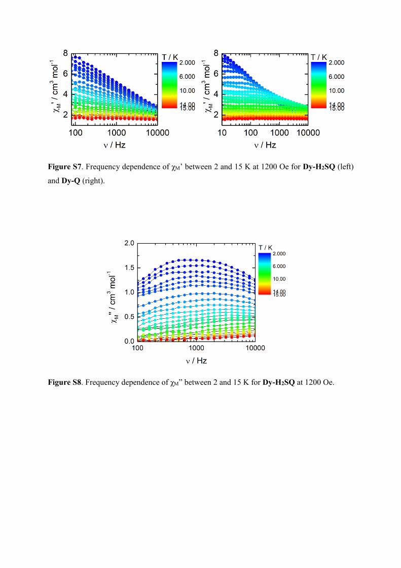
Figure S7. Frequency dependence of χM’ between 2 and 15 K at 1200 Oe for Dy-H2SQ (left)

and Dy-Q (right).

Figure S8. Frequency dependence of χM” between 2 and 15 K for Dy-H2SQ at 1200 Oe.

Extended Debye model.

1

1 2 2

1

1 2 2

1 sin2

'

1 2 sin2

cos2

''

1 2 sin2

M S T S

M T S

With T the isothermal susceptibility, S the adiabatic susceptibility, τ the relaxation time and α

an empiric parameter which describe the distribution of the relaxation time. For SMM with only

one relaxation time, α is close to zero. The extended Debye model was applied to fit

simultaneously the experimental variations of M’ and M’’ with the frequency of the

oscillating field ( 2 ). Typically, only the temperatures for which a maximum on the ’’

vs. f curves, have been considered. The best fitted parameters τ, α, T, S are listed in Table S2

with the coefficient of determination R².

Figure S9. Frequency dependence of the in-phase (M’) and out-of-phase (M”) components of

the ac susceptibility measured on powder at 4 K and 1200 Oe with the best fitted curves (red

lines) for Dy-Q.

Figure S10. Normalized Argand plot for Dy-Q between 2 and 5 K.

Table S1. X-ray crystallographic data of Dy-H2SQ and Dy-Q.

Compounds Dy-H2SQ Dy-Q

Formula C84H66Dy2F18O16S10 C86H68Cl4Dy2F18O16S10

M / g.mol-1 2318.96 2486.8

Crystal system Monoclinic Monoclinic

Space group C2/c (N°15) P21/c (N°14)

Cell parameters

a = 18.052(3) Å

b = 35.748(6) Å

c = 18.254(3) Å

β = 92.984(7) °

a = 10.6086(11) Å

b = 23.485(2) Å

c = 19.414(2) Å

β = 91.767(4) °

Volume / Å3 11763(4) 4834.6(9)

Z 4 2

T / K 150 (2) 150 (2)

2θ range /° 4.10 ≤ 2θ ≤ 55.45 5.87 ≤ 2θ ≤ 54.97

calc / g.cm-3 1.309 1.708

µ / mm-1 1.516 1.957

Number of

reflections

62737 191400

Independent

reflections

13532 11074

Fo2 > 2(Fo)2 9529 9273

Number of variables 544 526

Rint, R1, wR2 0.0661, 0.0981, 0.2764 0.1219, 0.0753, 0.1607

Table S2. Best fitted parameters (T, S, and α) with the extended Debye model Dy-Q at

1200 Oe in the temperature range 2-5.5 K.

T / K T / cm3 mol-1 S / cm3 mol-1 / s R²

2 9.87881 1.17843 0.47995 8.63066E-4 0.99731

2.2 9.6154 1.19238 0.46333 7.87665E-4 0.99905

2.4 9.11006 1.15028 0.45241 6.47181E-4 0.99945

2.6 8.42987 1.20621 0.41621 4.94235E-4 0.9987

2.8 8.21404 1.14112 0.41664 4.26137E-4 0.99939

3 7.56272 1.21513 0.37697 3.15642E-4 0.9989

3.5 6.71038 1.14576 0.36022 1.7472E-4 0.999

4 5.94654 1.26262 0.33113 9.66868E-5 0.99907

4.5 5.47045 1.16678 0.35391 5.23862E-5 0.99926

5 4.89902 1.44341 0.31628 3.24582E-5 0.99969

5.5 4.58454 1.27329 0.37174 1.65915E-5 0.99981

Table S3. Computed energies, g-tensor and wavefunction composition of the ground state

doublets in the effective spin ½ model for Dy-H2SQ.

KD E / cm-1 gX gY gZ Wavefunction*

1 0 0.11 1.10 15.08 34% |±13/2> + 25% |±15/2> +15% |±11/2> + 10% |±7/2>

2 13 0.03 1.11 14.29 26% |±11/2> + 18% |±13/2> +17% |±9/2> + 11% |±7/2>

3 155 1.92 2.18 14.69 38% |±9/2> + 19% |±15/2> +17% |±11/2> + 16% |±7/2>

4 228 2.92 5.15 11.23 24% |±5/2> + 17% |±3/2> +17% |±11/2> + 13% |±1/2>

5 274 2.22 4.32 11.93 23% |±7/2> + 18% |±3/2> +18% |±1/2> + 14% |±5/2>

6 352 0.55 1.20 16.04 31% |±15/2> + 24% |±13/2> +11% |±11/2>

7 400 10.40 8.05 0.39 50% |±1/2> + 15% |±3/2> +14% |±7/2>

8 413 10.35 8.12 0.04 32% |±3/2> + 28% |±5/2> +11% |±7/2> + 11% |±9/2> *: only components > 10% are given for sake of clarity

Table S4. Computed energies, g-tensor and wavefunction composition of the ground state

doublet in the effective spin ½ model for Dy-Q.

KD E / cm-1 gX gY gZ Wavefunction*

1 0 0.05 0.11 19.24 90% |±15/2>

2 80 0.14 0.26 15.86 70% |±13/2>

3 137 0.07 0.53 13.57 27% |±11/2> + 14% |±13/2> +13% |±7/2> + 12% |±5/2>

4 184 1.52 2.14 10.85 25% |±11/2> + 23% |±9/2> +19% |±5/2> + 15% |±1/2>

5 227 4.22 6.52 10.97 33% |±3/2> + 17% |±1/2> +15% |±7/2> + 13% |±5/2>

6 335 0.02 0.58 16.50 49% |±1/2> + 18% |±3/2> +11% |±9/2>

7 405 0.63 3.13 14.70 30% |±7/2> + 29% |±9/2> +12% |±3/2>

8 421 0.41 3.78 15.45 42% |±5/2> + 20% |±3/2> +18% |±7/2> + 11% |±11/2> *: only components > 10% are given for sake of clarity