Recursive Partitioning and Applications Heping Zhang Department of Epidemiology and Public Health Yale University School of Medicine June–July, 2011 This PDF slides cover Chapters 1–4, 6, 8, and 9 in the book of Heping Zhang and Burton Singer entitled “Recursive Partitioning and Applications" published by Springer in 2010. The instructors and students are assumed to have some acess to the book. Heping Zhang (C 2 S 2 , Yale University) UHK and NENU 1 / 186

Welcome message from author
This document is posted to help you gain knowledge. Please leave a comment to let me know what you think about it! Share it to your friends and learn new things together.
Transcript

Recursive Partitioning and Applications
Heping Zhang
Department of Epidemiology and Public HealthYale University School of Medicine
June–July, 2011
This PDF slides cover Chapters 1–4, 6, 8, and 9 in the book of Heping Zhang and Burton Singer entitled “Recursive Partitioning
and Applications" published by Springer in 2010. The instructors and students are assumed to have some acess to the book.
Heping Zhang (C2S2, Yale University) UHK and NENU 1 / 186

Outline
1 Introduction
2 A Practical Guide to Tree Construction
3 Logistic Regression
4 Classification Trees for a Binary Response
5 Forests
6 Censored Data
7 Survival Trees and Random Forests
Heping Zhang (C2S2, Yale University) UHK and NENU 2 / 186

Regression Model
Many scientific problems reduce to modeling the relationshipbetween two sets of variables. Regression methodology isdesigned to quantify these relationships.
linear regression for continuous datalogistic regression for binary dataproportional hazard regression for censored survival datamixed-effect regression for longitudinal data
These parametric (or semiparametric) regression methods maynot lead to faithful data descriptions when the underlyingassumptions are not satisfied.
Heping Zhang (C2S2, Yale University) UHK and NENU 3 / 186

Recursive Partitioning Based Methods
Nonparametric regression has evolved to relax or remove therestrictive assumptions.Recursive partitioning provides a useful alternative to theparametric regression methods.
Classification and Regression Trees (CART)Multivariate Adaptive Regression Splines (MARS)ForestSurvival Trees
Heping Zhang (C2S2, Yale University) UHK and NENU 4 / 186

Areas of Applications
financial firmsbanking crises (Cashin and Duttagupta 2008)credit cards (Altman 2002; Frydman, Altman and Kao 2002; Kumarand Ravi 2008)investments (Pace 1995 and Brennan, Parameswaran et al. 2001)
manufacturing and marketing companies (Levin, Zahavi, andOlitsky 1995; Chen and Su 2008)pharmaceutical industries (Chen et al. 1998)engineering research
natural language speech recognition (Bahl et al. 1989)musical sounds (Wieczorkowska 1999)text recognition (Desilva and Hull 1994)tracking roads in satellite images (Geman and Jedynak 1996)
Heping Zhang (C2S2, Yale University) UHK and NENU 5 / 186

Areas of Applications
astronomy (Owens, Griffiths, and Ratnatunga 1996)computers and the humanities (Shmulevich et al. 2001)chemistry (Chen, Rusinko, and Young 1998)environmental entomology (Hebertson and Jenkins 2008)forensics (Appavu and Rajaram 2008)polar biology (Terhune et al. 2008).
Heping Zhang (C2S2, Yale University) UHK and NENU 6 / 186

Biomedical Applications
Is this patient with chest pain suffering a heart attack?Does he simply have a strained muscle?
Heping Zhang (C2S2, Yale University) UHK and NENU 7 / 186

Examples
Chest PainGoldman et al. (1982, 1996): Build an expert computer system thatcould assist physicians in emergency rooms to classify patientswith chest pain into relatively homogeneous groups within a fewhours of admission using the clinical factors available.The authors included 10,682 patients with acute chest pain in thederivation data set and 4,676 in the validation data set.
ComaLevy et al. (1985): Predict the outcome from coma caused bycerebral hypoxia-ischemiathey studied 210 patients with cerebral hypoxia-ischemia andconsidered 13 factors including age, sex, verbal and motorresponses, and eye opening movement.
Heping Zhang (C2S2, Yale University) UHK and NENU 8 / 186
Gene Expression
Zhang et al. (2001) analyzed a data set from the expressionprofiles2,000 genes in 22 normal and 40 colon cancer tissues (Alon et al.1999).
Heping Zhang (C2S2, Yale University) UHK and NENU 9 / 186

Gene Expression
&%'$node 1C: 40N: 22
IL-8> 60
node 2C: 0N: 14
������
HHHHH
H
&%'$node 3C: 40N: 8
CANX> 290
&%'$node 4C: 10N: 8
RAB3B> 770
������
node 5C: 30N: 0
HHH
HHH
node 6C: 10N: 1
node 7C: 0N: 7
����
��
HHHH
HH
Heping Zhang (C2S2, Yale University) UHK and NENU 10 / 186

Statistical Problem
an outcome variable, Y, and a set of p predictors, x1, . . . , xp.
establish a relationship between Y and the x’sIP{Y = y | x1, . . . , xp},parametric models
exp(β0 +∑p
i=1 βixi)
1 + exp(β0 +∑p
i=1 βixi),
1√2π
exp[− (y− µ)2
2σ2
], µ = β0 +
p∑i=1
βixi.
Heping Zhang (C2S2, Yale University) UHK and NENU 11 / 186

Statistical Problem
Table: Correspondence Between the Uses of Classic Approaches andRecursive Partitioning Technique in This Book
Type ofParametric methods
Recursive partitioningresponse technique
Ordinary linear Regression trees andContinuous regression adaptive splines
BinaryLogistic regression Classification trees and
forests
CensoredProportion hazard Survival treesregressionMixed-effects models Regression trees and
Longitudinal adaptive splinesMultiple Exponential, marginal, Classification treesdiscrete and frailty models
Heping Zhang (C2S2, Yale University) UHK and NENU 12 / 186

Yale Pregnancy Outcome Study
PI: Dr. Michael B. Bracken at Yale University.Population: women who made a first prenatal visit to a privateobstetrics or midwife practice, health maintenance organization, orhospital clinic in the greater New Haven, Connecticut, area,between May 12, 1980, and March 12, 1982, and who anticipateddelivery at the Yale–New Haven Hospital.Sample size: a subset of 3,861 women whose pregnancies endedin a singleton live birth.Outcome: preterm delivery
Heping Zhang (C2S2, Yale University) UHK and NENU 13 / 186

Yale Pregnancy Outcome Study
Table: A List of Candidate Predictor Variables
Variable name Label Type Range/levelsMaternal age x1 Continuous 13–46Marital status x2 Nominal Currently married, divorced,
separated, widowed, never marriedRace x3 Nominal White, Black, Hispanic, Asian, othersMarijuana use x4 Nominal Yes, noTimes of using x5 Ordinal >= 5, 3–4, 2, 1 (daily), 4–6,marijuana 1–3 (weekly), 2–3, 1, < 1 (monthly)Years of education x6 Continuous 4–27Employment x7 Nominal Yes, noSmoker x8 Nominal Yes, noCigarettes smoked x9 Continuous 0–66Passive smoking x10 Nominal Yes, noGravidity x11 Ordinal 1–10Hormones/DES x12 Nominal None, hormones, DES,used by mother both, uncertainAlcohol (oz/day) x13 Ordinal 0–3Caffeine (mg) x14 Continuous 12.6–1273Parity x15 Ordinal 0–7
Heping Zhang (C2S2, Yale University) UHK and NENU 14 / 186

The Elements of Tree
root node: the circle on the top.internal nodeterminal nodesleft and right daughter nodesoffspring nodessplit
Heping Zhang (C2S2, Yale University) UHK and NENU 15 / 186

Interpretation of Tree
What are the contents of the nodes?Why and how is a parent node split into two daughter nodes?When do we declare a terminal node?
Heping Zhang (C2S2, Yale University) UHK and NENU 16 / 186

Interpretation of Tree
The root node contains a sample of subjects from which the tree isgrown–learning sample.The root node contains all 3,861 pregnant women.All nodes in the same layer constitute a partition of the root node.Every node in a tree is merely a subset of the learning sample.
Heping Zhang (C2S2, Yale University) UHK and NENU 17 / 186

An Example of Tree
����Root node
x13 > c2?no yes
����
x1 > c1?no yes
Internal node
I
II III
���+
QQQs
���+
QQQs
a
I
IIx13
c2
bbbb bbb bb bb b
c1 x1III
b bb bbb bbbb
b b bb
bb bb bbr rrr rrr rr r
b
Heping Zhang (C2S2, Yale University) UHK and NENU 18 / 186

Aim of Recursive Partitioning
Produce the terminal nodes that are homogeneousThey contain either dots or circles
Heping Zhang (C2S2, Yale University) UHK and NENU 19 / 186

Splitting a Node
Consider the variable x1 (age)32 distinct age values in the range of 13 to 4632-1=31 allowable splitsFor an ordinal predictor, the number of allowable splits is onefewer than the number of its distinctly observed values.
Heping Zhang (C2S2, Yale University) UHK and NENU 20 / 186

Allowable Splits
Table: Race
Left daughter node Right daughter nodeWhite Black, Hispanic, Asian, othersBlack White, Hispanic, Asian, othersHispanic White, Black, Asian, othersAsian White, Black, Hispanic, othersWhite, Black Hispanic, Asian, othersWhite, Hispanic Black, Asian, othersWhite, Asian Black, Hispanic, othersBlack, Hispanic White, Asian, othersBlack, Asian White, Hispanic, othersHispanic, Asian White, Black, othersBlack, Hispanic, Asian White, othersWhite, Hispanic, Asian Black, othersWhite, Black, Asian Hispanic, othersWhite, Black, Hispanic Asian, othersWhite, Black, Hispanic, Asian Others
Heping Zhang (C2S2, Yale University) UHK and NENU 21 / 186

Splits of a Nominal Variable
Race has 5 levels25−1 − 1 = 15 allowable splitsany nominal variable that has k levels contributes 2k−1 − 1allowable splits
Heping Zhang (C2S2, Yale University) UHK and NENU 22 / 186

Allowable Splits
The 15 predictors yield 347 possible splitsHow do we select one or several preferred splits from the pool ofallowable splits?We need to define a selection criterion
Heping Zhang (C2S2, Yale University) UHK and NENU 23 / 186

Goodness of Split
The goodness of a split must weigh the homogeneities (or theimpurities) in the two daughter nodes.Consider the question “Is x1 > c?”
Term PretermLeft Node (τL) x1 ≤ c n11 n12 n1·
Right Node (τR) x1 > c n21 n22 n2·n·1 n·2
Heping Zhang (C2S2, Yale University) UHK and NENU 24 / 186

Entropy Impurity
Left node
i(τL) = −n11
n1·log(
n11
n1·
)− n12
n1·log(
n12
n1·
).
Right node
i(τR) = −n21
n2·log(
n21
n2·
)− n22
n2·log(
n22
n2·
).
The goodness of a split, s, is measured by
∆I(s, τ) = i(τ)− IP{τL}i(τL)− IP{τR}i(τR).
τ is the parent node of τL and τR. IP{τL} and IP{τR} are the proportionsof the observations assigned to the left and right daughter nodes,
respectively.
Heping Zhang (C2S2, Yale University) UHK and NENU 25 / 186

Goodness of Split for Age Split at 35
Term PretermLeft Node (τL) 3521 198 3719
Right Node (τR) 135 7 1423656 205 3861
i(τL) = −35213719
log(35213719
)− 1983719
log(1983719
) = 0.2079.
i(τR) = 0.1964, i(τ) = 0.20753.
∆I(s, τ) = 0.00001.
Heping Zhang (C2S2, Yale University) UHK and NENU 26 / 186

The Goodness of Allowable Age Splits
Split Impurity 1000∆Ivalue Left node Right node
13 0.00000 0.20757 0.0114 0.00000 0.20793 0.1415 0.31969 0.20615 0.1716 0.27331 0.20583 0.1317 0.27366 0.20455 0.2318 0.31822 0.19839 1.1319 0.30738 0.19508 1.4020 0.28448 0.19450 1.1521 0.27440 0.19255 1.1522 0.26616 0.18965 1.2223 0.25501 0.18871 1.0524 0.25747 0.18195 1.5025 0.24160 0.18479 0.9226 0.23360 0.18431 0.7227 0.22750 0.18344 0.5828 0.22109 0.18509 0.37
Split Impurity 1000∆Ivalue Left node Right node
29 0.21225 0.19679 0.0630 0.20841 0.20470 0.0031 0.20339 0.22556 0.0932 0.20254 0.23871 0.1833 0.20467 0.23524 0.0934 0.20823 0.19491 0.0135 0.20795 0.19644 0.0136 0.20744 0.21112 0.0037 0.20878 0.09804 0.1838 0.20857 0.00000 0.3739 0.20805 0.00000 0.1840 0.20781 0.00000 0.1041 0.20769 0.00000 0.0642 0.20761 0.00000 0.0343 0.20757 0.00000 0.01
Heping Zhang (C2S2, Yale University) UHK and NENU 27 / 186

The Largest Goodness of Split from All Predictors
Variable x1 x2 x3 x4 x5 x6 x7 x81000∆I 1.5 2.8 4.0 0.6 0.6 3.2 0.7 0.6Variable x9 x10 x11 x12 x13 x14 x151000∆I 0.7 0.2 1.8 1.1 0.5 0.8 1.2
Heping Zhang (C2S2, Yale University) UHK and NENU 28 / 186

Things to Notice
The greatest reduction in the impurity comes from the age split at24.What about the age split at age 19, stratifying the study sampleinto teenagers and adults?This best age split is used to compete with the best splits from theother 14 predictors.The best of the best comes from the race variable with1000∆I = 4.0, i.e., ∆I = 0.004.
This best split divides the root node according to whether apregnant woman is Black or not.
Heping Zhang (C2S2, Yale University) UHK and NENU 29 / 186

Top Splits
����
1
����
2 ����
3Is she Black?
Yes No���+
QQQs
a
����
1
����
2 ����
3Is she Black?
Yes No
����
4 ����
5
Is sheemployed?
Yes No
���+
QQQs
���+
QQQs
b
Heping Zhang (C2S2, Yale University) UHK and NENU 30 / 186
Recursive Partitioning
After splitting the root node, we continue to divide its two daughternodes.The partition of node 2 uses only 710 Black women, and theremaining 3,151 non-Black women are put aside.The pool of allowable splits is nearly intact except that race doesnot contribute any more splits, as everyone is now Black.The total number of allowable splits decreases from 347 to at least332.An offspring node may use the same splitting variable as itsancestors.The number of allowable splits decreases as the partitioningcontinues.
Heping Zhang (C2S2, Yale University) UHK and NENU 31 / 186

Important Issues
If all candidate variables are equally plausible substantively, thengenerate separate trees using each of the variables to continuethe splitting process.If only one or two of the candidate variables is interpretable in thecontext of the classification problem at hand, then select them foreach of two trees to continue the splitting process.
Heping Zhang (C2S2, Yale University) UHK and NENU 32 / 186

Terminal Nodes
The recursive partitioning process may proceed until the tree issaturated in the sense that the offspring nodes subject to furtherdivision cannot be split.
there is only one subject in a node.the total number of allowable splits for a node drops as we movefrom one layer to the next.the number of allowable splits eventually reduces to zerothe nodes are terminal when they are not divided further
Heping Zhang (C2S2, Yale University) UHK and NENU 33 / 186

Stopping Rules and Tree Pruning
The saturated tree is usually too large to be useful.
the terminal nodes are so small that we cannot make sensiblestatistical inference.this level of detail is rarely scientifically interpretable.a minimum size of a node is set a priori.stopping rules
Automatic Interaction Detection(AID) (Morgan and Sonquist 1963)declares a terminal node based on the relative merit of its best splitto the quality of the root node
Breiman et al. (1984, p. 37) argued that depending on thestopping threshold, the partitioning tends to end too soon or toolate.pruning
find a subtree of the saturated tree that is most “predictive" of theoutcome and least vulnerable to the noise in the data.
Heping Zhang (C2S2, Yale University) UHK and NENU 34 / 186
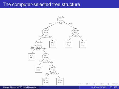
The computer-selected tree structure
NPT=205
N=3861
Race
NPT=135
N=3151
# ofPregnancies > 4
NPT=70
N=710
Employed
NPT=118
N=2980
Hormones/DES use
NPT=17
N=171
NPT=59
N=512
NPT=11
N=198
NPT=8
N=61
NPT=110
N=2919
Years ofeducation > 12
NPT=51
N=983
NPT=59
N=1936
Age > 32
NPT=41
N=1602
NPT=18
N=334
BlacksOthers
YesNo YesNo
OthersDES orboth orNA
Yes orNA
No
YesNo
Heping Zhang (C2S2, Yale University) UHK and NENU 35 / 186
Interpretation
Let us examine the left node in the third layer
2,980 non-Black women who had no more than four pregnanciesThe split for this group of women is based on their mothers’ use ofhormones and/or DESIf their mothers used hormones and/or DES, or the answers werenot reported, they are assigned to the left daughter node.The right daughter node consists of those women whose mothersdid not use hormones or DES, or who reported uncertainty abouttheir mothers’ use.Women with the “uncertain” answer and the missing answer areassigned to different sides of the parent node.We need to manually change the split.Numerically, the goodness of split, ∆, changes from 0.00176 to0.00148.
Heping Zhang (C2S2, Yale University) UHK and NENU 36 / 186

Revised tree structure
N=3861RR=2.14
CI=1.62-2.82
Race
N=3151RR=2.53
CI=1.48-4.31
# ofPregnancies
> 4
N=710RR=1.13
CI=0.67-1.89
Employed
N=2980RR=1.82
CI=0.93-3.57
Hormones/DES use
NPT=17
N=171
NPT=59
N=512
NPT=11
N=198
NPT=112
N=2949
NPT=6
N=31
BlacksOthers
YesNo YesNo
DES or BothOthers
Heping Zhang (C2S2, Yale University) UHK and NENU 37 / 186

Risk profile
Who were at risk of preterm delivery?
non-Black women who have four or fewer prior pregnancies andwhose mothers used DES and/or other hormones are at highestrisk19.4% of these women have preterm deliveries as opposed to3.8% whose mothers did not use DESamong Black women who are also unemployed, 11.5% hadpreterm deliveries, as opposed to 5.5% among employed Blackwomenemployment status may just serve as a proxy for more biologicalcircumstances
Heping Zhang (C2S2, Yale University) UHK and NENU 38 / 186

Regression Model
Logistic regression is a standard approach to the analysis of binarydata. For every study subject i we assume that the response Yi has theBernoulli distribution
P{Yi = yi} = θyii (1− θi)
1−yi , yi = 0, 1, i = 1, . . . , n,
where the parametersθ = (θ1, . . . , θn)′
must be estimated from the data. Here, a prime denotes the transposeof a vector or matrix.
Heping Zhang (C2S2, Yale University) UHK and NENU 39 / 186

Link Function
To model these data, we generally attempt to reduce the n parametersin θ to fewer degrees of freedom. The unique feature of logisticregression is to accomplish this by introducing the logit link function:
θi =exp(β0 +
∑pj=1 βjxij)
1 + exp(β0 +∑p
j=1 βjxij),
whereβ = (β0, β1, . . . , βp)′
is the new (p + 1)-vector of parameters to be estimated and(xi1, . . . , xip) are the values of the p covariates included in the model forthe ith subject (i = 1, . . . , n).
Heping Zhang (C2S2, Yale University) UHK and NENU 40 / 186

Likelihood
To estimate β, we make use of the likelihood function
L(β; y)
=
n∏i=1
[exp(β0 +
∑pj=1 βjxij)
1 + exp(β0 +∑p
j=1 βjxij)
]yi[
11 + exp(β0 +
∑pj=1 βjxij)
]1−yi
=
∏yi=1 exp(β0 +
∑pj=1 βjxij)∏n
i=1[1 + exp(β0 +∑p
j=1 βjxij)].
By maximizing L(β; y), we obtain the maximum likelihood estimate β ofβ.
Heping Zhang (C2S2, Yale University) UHK and NENU 41 / 186

Odds Ratio
The odds that the ith subject has an abnormal condition is
θi
1− θi= exp(β0 +
p∑j=1
βjxij).
Consider two individuals i and k for whom xi1 = 1, xk1 = 0, and xij = xkj
for j = 2, . . . , p. Then, the odds ratio for subjects i and k to be abnormalis
θi/(1− θi)
θk/(1− θk)= exp(β1).
Taking the logarithm of both sides, we see that β1 is the log odds ratioof the response resulting from two such subjects when their firstcovariate differs by one unit and the other covariates are the same.
Heping Zhang (C2S2, Yale University) UHK and NENU 42 / 186

Revisit of the Pregnancy Example
Three predictors, x2 (marital status), x3 (race), and x12 (hormones/DESuse), are nominal and have five levels.
Heping Zhang (C2S2, Yale University) UHK and NENU 43 / 186

Dummy Variable for Marital Status
Let
z1 =
{1 if a subject was currently married,0 otherwise,
z2 =
{1 if a subject was divorced,0 otherwise,
z3 =
{1 if a subject was separated,0 otherwise,
z4 =
{1 if a subject was widowed,0 otherwise.
Heping Zhang (C2S2, Yale University) UHK and NENU 44 / 186

Dummy Variable for Race
z5 =
{1 for a Caucasian,0 otherwise,
z6 =
{1 for an African-American,0 otherwise,
z7 =
{1 for a Hispanic,0 otherwise,
z8 =
{1 for an Asian,0 otherwise,
Heping Zhang (C2S2, Yale University) UHK and NENU 45 / 186
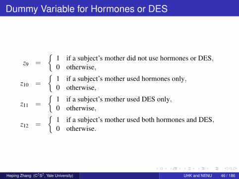
Dummy Variable for Hormones or DES
z9 =
{1 if a subject’s mother did not use hormones or DES,0 otherwise,
z10 =
{1 if a subject’s mother used hormones only,0 otherwise,
z11 =
{1 if a subject’s mother used DES only,0 otherwise,
z12 =
{1 if a subject’s mother used both hormones and DES,0 otherwise.
Heping Zhang (C2S2, Yale University) UHK and NENU 46 / 186

Variable Selection
Table: MLE for an Initially Selected Model
Selected Degrees of Coefficient Standardvariable freedom Estimate Error p-value
Intercept 1 −2.172 0.6912 0.0017x1(age) 1 0.046 0.0218 0.0356
z6(Black) 1 0.771 0.2296 0.0008x6(educ.) 1 −0.159 0.0501 0.0015
z10(horm.) 1 1.794 0.5744 0.0018
The model selection is based on the observations with completeinformation in all predictors even though fewer predictors areconsidered in later steps.
Heping Zhang (C2S2, Yale University) UHK and NENU 47 / 186

Variable Selection
x7 (employment) and x8 (smoking) were not selected and had most ofthe missing data, and hence removed from the selection.
Table: MLE for a Revised Model
Selected Degrees of Coefficient Standardvariable freedom Estimate Error p-value
Intercept 1 −2.334 0.4583 0.0001x6(educ.) 1 −0.076 0.0313 0.0151z6(Black) 1 0.705 0.1688 0.0001x11(grav.) 1 0.114 0.0466 0.0142
z10(horm.) 1 1.535 0.4999 0.0021
Heping Zhang (C2S2, Yale University) UHK and NENU 48 / 186

Final Model
Table: MLE for the Final Model
Selected Degrees of Coefficient Standardvariable freedom Estimate Error p-value
Intercept 1 −2.344 0.4584 0.0001x6(educ.) 1 −0.076 0.0313 0.0156z6(Black) 1 0.699 0.1688 0.0001x11(grav.) 1 0.115 0.0466 0.0137
z10 (horm.) 1 1.539 0.4999 0.0021
Heping Zhang (C2S2, Yale University) UHK and NENU 49 / 186

Comparison of the Initial and Final Fits
Selected Degrees of Coefficient Standardvariable freedom Estimate Error p-value
Intercept 1 −2.334 0.4583 0.0001x6(educ.) 1 −0.076 0.0313 0.0151z6(Black) 1 0.705 0.1688 0.0001x11(grav.) 1 0.114 0.0466 0.0142
z10(horm.) 1 1.535 0.4999 0.0021Intercept 1 −2.344 0.4584 0.0001x6(educ.) 1 −0.076 0.0313 0.0156z6(Black) 1 0.699 0.1688 0.0001x11(grav.) 1 0.115 0.0466 0.0137
z10 (horm.) 1 1.539 0.4999 0.0021
Heping Zhang (C2S2, Yale University) UHK and NENU 50 / 186

Interactions
Two-way interactions between the selected variables wereexamined.The backward stepwise procedure was run again.No interaction terms were significant at the level of 0.05.The final model does not include any interaction.
Heping Zhang (C2S2, Yale University) UHK and NENU 51 / 186

Interpretation
The odds ratio for a Black woman (z6) to deliver a premature infantis doubled relative to that for a White woman, because thecorresponding odds ratio equals exp(0.699) ≈ 2.013..The use of DES by the mother of the pregnant woman (z10) has asignificant and enormous effect on the preterm delivery.Years of education (x6), however, seems to have a small, butsignificant, protective effect.Finally, the number of previous pregnancies (x11) has a significant,but low-magnitude negative effect on the preterm delivery.
Heping Zhang (C2S2, Yale University) UHK and NENU 52 / 186

Interpretation
The odds ratio for a Black woman (z6) to deliver a premature infantis doubled relative to that for a White woman, because thecorresponding odds ratio equals exp(0.699) ≈ 2.013.
The use of DES by the mother of the pregnant woman (z10) has asignificant and enormous effect on the preterm delivery.Years of education (x6), however, seems to have a small, butsignificant, protective effect.Finally, the number of previous pregnancies (x11) has a significant,but low-magnitude negative effect on the preterm delivery.
Heping Zhang (C2S2, Yale University) UHK and NENU 53 / 186

Impact of Missing Data
Selected Degrees of Coefficient Standardvariable freedom Estimate Error p-value
Intercept 1 −2.172 0.6912 0.0017x1(age) 1 0.046 0.0218 0.0356
z6(Black) 1 0.771 0.2296 0.0008x6(educ.) 1 −0.159 0.0501 0.0015
z10(horm.) 1 1.794 0.5744 0.0018Intercept 1 −2.344 0.4584 0.0001x6(educ.) 1 −0.076 0.0313 0.0156z6(Black) 1 0.699 0.1688 0.0001x11(grav.) 1 0.115 0.0466 0.0137
z10 (horm.) 1 1.539 0.4999 0.0021
Heping Zhang (C2S2, Yale University) UHK and NENU 54 / 186

Impact of Missing Data
Missing data may lead to serious loss of information.We may end up with imprecise or even false conclusions.Variables change in the selected models.The estimated coefficients can be notably different.
Heping Zhang (C2S2, Yale University) UHK and NENU 55 / 186

Predictive Performance
false-positive errorsfalse-negative errorsreceiver operating characteristic (ROC) curve plots true-positiveprobability (y-axis) against false-positive probability (x-axis)true positive probability: sensitivitytrue negative probability: specificity
Heping Zhang (C2S2, Yale University) UHK and NENU 56 / 186

The computer-selected tree structure
1-specificity
sens
itivi
ty
0.0 0.2 0.4 0.6 0.8 1.0
0.0
0.2
0.4
0.6
0.8
1.0
Heping Zhang (C2S2, Yale University) UHK and NENU 57 / 186

Node Impurity
Intuitively, the least impure node should have only one class ofoutcome (i.e., IP{Y = 1 | τ} = 0 or 1), and its impurity is zero.Node τ is most impure when IP{Y = 1 | τ} = 1
2 .
The impurity function has a concave shape and can be formallydefined as
i(τ) = φ({Y = 1 | τ}),
where the function φ has the properties (i) φ ≥ 0 and (ii) for anyp ∈ (0, 1), φ(p) = φ(1− p) and φ(0) = φ(1) < φ(p).
Heping Zhang (C2S2, Yale University) UHK and NENU 58 / 186

Common Choices of Node Impurity
φ(p) = min(p, 1− p), (Bayes or the minimum error)φ(p) = −p log(p)− (1− p) log(1− p), (entropy)φ(p) = p(1− p), (Gini index)
where 0 log 0 = 0.Devroye et al. (1996, p. 29) call these φ’s the F-errors.
Heping Zhang (C2S2, Yale University) UHK and NENU 59 / 186

Impurity Functions
-
6
0
12
12 1 p
Impurity
������@
@@@@@
������
�����
������
Minimum ErrorEntropy
Gini
Heping Zhang (C2S2, Yale University) UHK and NENU 60 / 186

Entropy and Likelihood
Suppose that Y in node τL follows a binomial distribution with afrequency of θ, namely,
IP{Y = 1 | τL} = θ.
The log-likelihood function from the n1· observations in node τL is
n11 log(θ) + n12 log(1− θ).
The maximum of this log-likelihood function is
n11 log(
n11
n1·
)+ n12 log
(n12
n1·
),
which is proportional to the entropy.
Heping Zhang (C2S2, Yale University) UHK and NENU 61 / 186

Determination of Terminal Nodes
For a tree T we define
R(T ) =∑τ∈T
IP{τ}r(τ),
where T is the set of terminal nodes of T .r(τ) measures a certain quality of node τ. It is similar to the sumof the squared residuals in the linear regression.The purpose of pruning is to select the best subtree, T ∗, of aninitially saturated tree, T0, such that R(T ) is minimized.
Heping Zhang (C2S2, Yale University) UHK and NENU 62 / 186

Misclassification Cost
Let c(i|j) be a unit misclassification cost that a class j subject isclassified as a class i subject.When i = j, we have the correct classification and the cost shouldnaturally be zero, i.e., c(i|i) = 0.
Without loss of generality we can set c(1|0) = 1.
The clinicians and the statisticians need to work together to gaugethe relative cost of c(0|1).
Heping Zhang (C2S2, Yale University) UHK and NENU 63 / 186

Misclassification Cost
Assumed Node numberClass 1 2 3 4 5
c(0|1) 1 3656 640 3016 187 4531 0 205 70 135 11 59
10 0 2050 700 1350 110 59018 0 3690 1260 2430 198 1062
Heping Zhang (C2S2, Yale University) UHK and NENU 64 / 186

Class Assignment
Node τ is assigned class j if∑i
[c(j|i)IP{Y = i | τ}] ≤∑
i
[c(1− j|i)IP{Y = i | τ}].
For example, when c(0|1) = 10, it means that one false-negative errorcounts as many as ten false-positive ones. The cost is 3656 if the rootnode is assigned class 1. It becomes 225× 10 = 2250 if the root nodeis assigned class 0. Therefore, the root node should be assigned class0 for 2250 < 3656.
Heping Zhang (C2S2, Yale University) UHK and NENU 65 / 186

Use of r(τ) for Splitting?
It is usually difficult to assign the cost function before any tree is grown.As a matter of fact, the assignment can still be challenging even whena tree profile is given.
Heping Zhang (C2S2, Yale University) UHK and NENU 66 / 186

Resubstitution Estimates of Misclassification Cost
Unit cost: c(0|1) = 10)Node Node Weight Within-node Cost
number class IP{τ} cost r(τ) Rs(τ)
1 0 38613861
10∗2053861
20503861 = 0.531
2 1 7103861
1∗640710
6403861 = 0.166
3 0 31513861
10∗1353151
13503861 = 0.35
4 0 1983861
10∗11198
1103861 = 0.028
5 1 5063861
1∗453506
4533861 = 0.117
Heping Zhang (C2S2, Yale University) UHK and NENU 67 / 186

Caveat of Resubstitution Estimates
Let Rs(τ) denote the resubstitution estimate of themisclassification cost for node τ.The resubstitution estimates generally underestimate the cost.If we have an independent data set, we can assign the newsubjects to various nodes of the tree and calculate the cost basedon these new subjects. This cost tends to be higher than theresubstitution estimate, because the split criteria are somehowrelated to the cost, and as a result, the resubstitution estimate ofmisclassification cost is usually overoptimistic.In some applications, such an independent data set, called a testsample or validation set, is available.
Heping Zhang (C2S2, Yale University) UHK and NENU 68 / 186
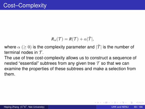
Cost–Complexity
Rα(T ) = R(T ) + α|T |,
where α (≥ 0) is the complexity parameter and |T | is the number ofterminal nodes in T .The use of tree cost-complexity allows us to construct a sequence ofnested “essential” subtrees from any given tree T so that we canexamine the properties of these subtrees and make a selection fromthem.
Heping Zhang (C2S2, Yale University) UHK and NENU 69 / 186

Cost–Complexity
Let T0, be the five-node tree. The cost for T0 is0.350 + 0.028 + 0.117 = 0.495 and its complexity is 3. Thus, itscost-complexity is 0.495 + 3α for a given complexity parameter α.Is there a subtree of T0 that has a smaller cost-complexity?
Theorem(Breiman et al. 1984, Section 3.3) For any value of the complexityparameter α, there is a unique smallest subtree of T0 that minimizesthe cost-complexity.
Heping Zhang (C2S2, Yale University) UHK and NENU 70 / 186

Cost–Complexity
We cannot have two subtrees of the smallest size and of the samecost-complexity.This smallest subtree is referred to as the optimal subtree withrespect to the complexity parameter.When α = 0, the optimal subtree is T0 itself.What are the other subtrees and their complexities?
Heping Zhang (C2S2, Yale University) UHK and NENU 71 / 186

Cost–Complexity
We can always choose α large enough that the correspondingoptimal subtree is the single-node tree.When α ≥ 0.018, T2 (the root node tree) becomes the optimalsubtree, because
R0.018(T2) = 0.531 + 0.018 ∗ 1 = 0.495 + 0.018 ∗ 3 = R0.018(T0)
and
R0.018(T2) = 0.531 + 0.018 ∗ 1 < 0.516 + 0.018 ∗ 2 = R0.018(T1).
Although R0.018(T2) = R0.018(T0), T2 is the optimal subtree, becauseit is smaller than T0.
This calculation confirms the theorem that we do not have twosubtrees of the smallest size and of the same cost-complexity.
Heping Zhang (C2S2, Yale University) UHK and NENU 72 / 186

Cost–Complexity
T1 is not an optimal subtree for any α.T0 is the optimal subtree for any α ∈ [0, 0.018) and T2 is the optimalsubtree when α ∈ [0.018,∞).
Not all subtrees are optimal with respect to a complexityparameter.Although the complexity parameter takes a continuous range ofvalues, we have only a finite number of subtrees.An optimal subtree is optimal for an interval range of thecomplexity parameter, and the number of such intervals has to befinite.
Heping Zhang (C2S2, Yale University) UHK and NENU 73 / 186

Nested Optimal Subtrees
We derive the first positive threshold parameter, α1, for this tree bycomparing the resubstitution misclassification cost of an internalnode to the sum of the resubstitution misclassification costs of itsoffspring terminal nodes.Note the sum of the resubstitution misclassification costs of itsoffspring terminal nodes denoted by Rs(Tτ ) for a node τ.
Heping Zhang (C2S2, Yale University) UHK and NENU 74 / 186

Nested Optimal Trees
����
#12050
2053656
����+
QQQQs
����
#31350
1353016
���+
QQQs
����
#2640
70640�
��+
QQQs
#4110
11187
#5453
59453 �������+
QQQs
#61180
1182862
#825
625
#91120
1122837
#7154
17154
Heping Zhang (C2S2, Yale University) UHK and NENU 75 / 186
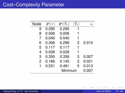
Cost–Complexity Parameter
Node Rs(τ) Rs(Tτ ) |Tτ | α
9 0.290 0.290 18 0.006 0.006 17 0.040 0.040 16 0.306 0.296 2 0.0105 0.117 0.117 14 0.028 0.028 13 0.350 0.336 3 0.0072 0.166 0.145 2 0.0211 0.531 0.481 5 0.013
Minimum 0.007
Heping Zhang (C2S2, Yale University) UHK and NENU 76 / 186
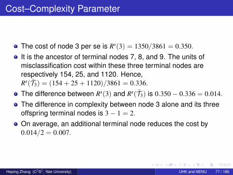
Cost–Complexity Parameter
The cost of node 3 per se is Rs(3) = 1350/3861 = 0.350.
It is the ancestor of terminal nodes 7, 8, and 9. The units ofmisclassification cost within these three terminal nodes arerespectively 154, 25, and 1120. Hence,Rs(T3) = (154 + 25 + 1120)/3861 = 0.336.
The difference between Rs(3) and Rs(T3) is 0.350− 0.336 = 0.014.
The difference in complexity between node 3 alone and its threeoffspring terminal nodes is 3− 1 = 2.
On average, an additional terminal node reduces the cost by0.014/2 = 0.007.
Heping Zhang (C2S2, Yale University) UHK and NENU 77 / 186

Consequence of Pruning
If we cut the offspring nodes of the root node, we have theroot-node tree whose cost-complexity is 0.531 + α.
For it to have the same cost-complexity as the initial nine-nodetree, we need 0.481 + 5α = 0.531 + α, giving α = 0.013.How about changing node 2 to a terminal node?
The initial nine-node tree is compared with a seven-node subtree,consisting of nodes 1 to 3, and 6 to 9.For the new subtree to have the same cost-complexity as the initialtree, we find α = 0.021.
In fact, for any internal node, τ 6∈ T , the value of α is precisely
Rs(τ)− Rs(Tτ )
|Tτ | − 1.
The first positive threshold parameter, α1, is the smallest α overthe |T | − 1 internal nodes.
Heping Zhang (C2S2, Yale University) UHK and NENU 78 / 186

A Pruned Tree
Using α1 we change an internal node τ to a terminal node when
Rs(τ) + α1 ≤ Rs(Tτ ) + α1|Tτ |
until this is not possible. This pruning process results in the optimalsubtree corresponding to α1.
����
1
����
2 ����
3Is she Black?
Yes No
����
4 ����
5
Is sheemployed?
Yes No
���+
QQQs
���+
QQQs
Heping Zhang (C2S2, Yale University) UHK and NENU 79 / 186

Nested Optimal Subtrees
After pruning the tree using the first threshold, we seek thesecond threshold complexity parameter, α2.
We knew from our previous discussion that α2 = 0.018 and itsoptimal subtree is the root-node tree. No more thresholds need tobe found from here, because the root-node tree is the smallestone.In general, suppose that we end up with m thresholds,0 < α1 < α2 < · · · < αm, and let α0 = 0.
Let the corresponding optimal subtrees beTα0 ⊃ Tα1 ⊃ Tα2 ⊃ · · · ⊃ Tαm , where Tα1 ⊃ Tα2 means that Tα2 is asubtree of Tα1 .
Heping Zhang (C2S2, Yale University) UHK and NENU 80 / 186

Nested Optimal Subtrees
TheoremIf α1 > α2, the optimal subtree corresponding to α1 is a subtree of theoptimal subtree corresponding to α2.
What’s next?We need a good estimate of R(Tαk) (k = 0, 1, . . . ,m), namely, themisclassification costs of the subtrees.We will select the one with the smallest misclassification cost.
Heping Zhang (C2S2, Yale University) UHK and NENU 81 / 186

Select the Optimal Subtree
When a test sample is available, estimating R(T ) for any subtreeT is straightforward, because we only need to apply the subtreesto the test sample.Difficulty arises when we do not have a test sample.The cross-validation process is generally used by creating artificialtest samples.Divide the entire study sample into a number of pieces, usually 5,10, or 25 corresponding to 5-, 10-, or 25-fold cross-validation,respectively.
Heping Zhang (C2S2, Yale University) UHK and NENU 82 / 186

Cross-validation
Heping Zhang (C2S2, Yale University) UHK and NENU 83 / 186

Cross-validation
Randomly divide the 3861 women into five groups: 1 to 5. Group1 has 773 women and each of the rest contains 772 women.Let L(−i) be the sample set including all but those subjects ingroup i, i = 1, . . . , 5.
Using the 3088 women in L(−1), produce another large tree, sayT(−1), in the same way as we did using all 3861 women.Take each αk from the sequence of complexity parameters as hasalready been derived above and obtain the optimal subtree,T(−1),k, of T(−1) corresponding to αk.
We have a sequence of the optimal subtrees of T(−1), i.e.,{T(−1),k}m
0 .
Using group 1 as a test sample relative to L(−1), we have anunbiased estimate, Rts(T(−1),k), of R(T(−1),k).
Heping Zhang (C2S2, Yale University) UHK and NENU 84 / 186

Cross-validation
Because T(−1),k is related to Tαk through the same αk, Rts(T(−1),k)can be regarded as a cross-validation estimate of R(Tαk).
Using L(−i) as the learning sample and the data in group i as thetest sample, we also have Rts(T(−i),k), (i = 2, . . . , 5) as thecross-validation estimate of R(Tαk).
The final cross-validation estimate, Rcv(Tαk), of R(Tαk) follows fromaveraging Rts(T(−i),k) over i = 1, . . . , 5.
Heping Zhang (C2S2, Yale University) UHK and NENU 85 / 186

Cross-validation
The subtree corresponding to the smallest Rcv is obviouslydesirable.The cross-validation estimates generally have substantialvariabilities.Breiman et al. (1984) proposed a revised strategy to select thefinal tree, which takes into account the standard errors of thecross-validation estimates.
Let SEk be the standard error for Rcv(Tαk ).Suppose that Rcv(Tαk∗ ) is the smallest among all Rcv(Tαk )’s.The revised selection rule selects the smallest subtree whosecross-validation estimate is within a prespecified range of Rcv(Tαk∗ ),which is usually defined by one unit of SEk∗ . This is the so-called1-SE rule.
Empirical evidence suggests that the tree selected with the 1-SErule is often superior to the one selected with the 0-SE rule.
Heping Zhang (C2S2, Yale University) UHK and NENU 86 / 186

Cross-validation
Every subject in the entire study sample was used once as atesting subject and was assigned a class membership m + 1 timesthrough the sequence of m + 1 subtrees built upon thecorresponding learning sample.Let Ci,k be the misclassification cost incurred for the ith subjectwhile it was a testing subject and the classification rule was basedon the kth subtree, i = 1, . . . , n, k = 0, 1, . . . ,m.
Rcv(Tαk) =∑
j=0,1 IP{Y = j}Ck|j, where Ck|j is the average of Ci,k
over the set Sj of the subjects whose response is j (i.e., Y = j).
Heping Zhang (C2S2, Yale University) UHK and NENU 87 / 186
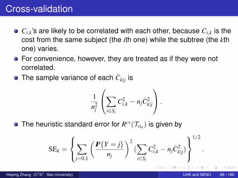
Cross-validation
Ci,k’s are likely to be correlated with each other, because Ci,k is thecost from the same subject (the ith one) while the subtree (the kthone) varies.For convenience, however, they are treated as if they were notcorrelated.The sample variance of each Ck|j is
1n2
j
∑i∈Sj
C2i,k − njC2
k|j
.
The heuristic standard error for Rcv(Tαk) is given by
SEk =
∑j=0,1
(IP{Y = j}
nj
)2
(∑i∈Sj
C2i,k − njC2
k|j)
1/2
.
Heping Zhang (C2S2, Yale University) UHK and NENU 88 / 186
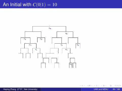
An Initial with C(0|1) = 10
Heping Zhang (C2S2, Yale University) UHK and NENU 89 / 186

Cross-validation estimates of MC
5- and 10-fold estimates are respectively indicated by • and +. Alsoplotted along the estimates are the intervals of length of two SEs..
•• • • • • •
• • •
•
The sequence of nested subtrees
Mis
clas
sific
atio
n co
st
1 3 5 7 9
0.45
0.50
0.55
0.60
0.65
++
++ +
+ +
++ +
+
Heping Zhang (C2S2, Yale University) UHK and NENU 90 / 186

Interpretation
The 1-SE rule selects the root-node subtree.The risk factors considered here may not have enough predictivepower to stand out and pass the cross-validation.This statement is obviously relative to the selected unit costC(0|1) = 10.
When we used C(0|1) = 18 and performed a 5-foldcross-validation, the final tree was different.
Heping Zhang (C2S2, Yale University) UHK and NENU 91 / 186

An Alternative Pruning Approach
The choice of the penalty for a false-negative error, C(0|1) = 10, isvital to the selection of the final tree structure.In many secondary analyses, however, the purpose is mainly toexplore the data structure and to generate hypotheses.It would be convenient to proceed with the analysis withoutassigning the unit of misclassification cost.Sometimes we cannot hold trees to a fixed algorithm.
Heping Zhang (C2S2, Yale University) UHK and NENU 92 / 186

An Alternative Pruning Approach
After the large tree T is grown, assign a statistic Sτ to eachinternal node τ from the bottom up.Align these statistics in increasing order as
Sτ1 ≤ Sτ2 ≤ · · · ≤ Sτ|T |−1.
Select a threshold level and change an internal node to a terminalone if its statistic is less than the threshold level.
Heping Zhang (C2S2, Yale University) UHK and NENU 93 / 186

An Alternative Pruning Approach
Locate the smallest Sτ over all internal nodes and prune theoffspring of the highest node(s) that reaches this minimum.What remains is the first subtree.Repeat the same process until the subtree contains the root nodeonly.As the process continues, a sequence of nested subtrees,T1, . . . , Tm, will be produced. To select a threshold value, we makea plot of minτ∈Ti−Ti
Sτ versus |Ti|, i.e., the minimal statistic of asubtree against its size.Look for a possible “kink” in this plot where the pattern changes.
Heping Zhang (C2S2, Yale University) UHK and NENU 94 / 186

A Roughly Pruned Tree
1
2
4
7
8
9 10
5 6
3
Heping Zhang (C2S2, Yale University) UHK and NENU 95 / 186

Maximum Statistic
Term PretermLeft Node 640 70 710
Right Node 3016 135 31513656 205 3861
Relative risk (RR) of preterm as (70/710)/(135/3151) = 2.3.
The standard error for the log RR is approximately√1/70− 1/710 + 1/135− 1/3151 = 0.141.
The Studentized log relative risk is 0.833/0.141 = 5.91.
Heping Zhang (C2S2, Yale University) UHK and NENU 96 / 186

Statistics for Internal Nodes
Node # 1 2 3 4 5Raw Statistic 5.91 2.29 3.72 1.52 3.64Max. Statistic 5.91 2.29 3.72 1.94 3.64
Node # 6 7 8 9 10Raw Statistic 1.69 1.47 1.35 1.94 1.60Max. Statistic 1.69 1.94 1.94 1.94 1.60
For each internal node we replace the raw statistic with themaximum of the raw statistics over its offspring internal nodes ifthe latter is greater.For instance, the raw value 1.52 is replaced with 1.94 for node 4;The maximum statistic has seven distinct values: 1.60, 1.69, 1.94,2.29, 3.64, 3.72, and 5.91, each of which results in a subtree.We have a sequence of eight nested subtrees.
Heping Zhang (C2S2, Yale University) UHK and NENU 97 / 186

The First Subtree
Tree 1
1
2
4
7
8
9
5 6
3
Heping Zhang (C2S2, Yale University) UHK and NENU 98 / 186

The Next Two Subtrees
Tree 2
1
2
4
7
8
9
3
5
Tree 3
1
2
5
3
Heping Zhang (C2S2, Yale University) UHK and NENU 99 / 186

The Next Four Subtrees
Tree 4
1
5
3
Tree 5
1
3
Tree 6
1 1
Tree 7
Heping Zhang (C2S2, Yale University) UHK and NENU 100 / 186

Tree Size vs Internal Node Statistics
2112
34
56
7
21
15.510 node statistics
treesize
Heping Zhang (C2S2, Yale University) UHK and NENU 101 / 186

Tree-Based vs Logistic Regression
The area under the curve is 0.622 for the tree-based model and 0.637for the logistic model
1-specificity
sens
itivi
ty
0.0 0.2 0.4 0.6 0.8 1.0
0.0
0.2
0.4
0.6
0.8
1.0
Heping Zhang (C2S2, Yale University) UHK and NENU 102 / 186

Use of Both Tree-Based and Logistic Regression:Approach I
Take the linear equation derived from the logistic regression as anew predictor.In the present application, the new predictor is defined asx16 = −2.344− 0.076x6 + 0.699z6 + 0.115x11 + 1.539z10.
Heping Zhang (C2S2, Yale University) UHK and NENU 103 / 186

The Final Tree
The equation from the logistic regression is used.
Heping Zhang (C2S2, Yale University) UHK and NENU 104 / 186

Conclusion
Education shows a protective effect, particularly for those withcollege or higher education.Age has merged as a risk factor. In the fertility literature, whethera women is at least 35 years old is a common standard forpregnancy screening.The risk of delivering preterm babies is not monotonic with respectto the combined score x16.
The risk is lower when −2.837 < x16 ≤ −2.299 than when−2.299 < x16 ≤ −2.062.
Heping Zhang (C2S2, Yale University) UHK and NENU 105 / 186

Use of Both Tree-Based and Logistic Regression:Approach II
Run the logistic regression after a tree is grown.Create five dummy variables, each of which corresponds to one ofthe five terminal nodes.
Variable label Specificationz13 Black, unemployedz14 Black, employedz15 non-Black, ≤ 4 pregnancies, DES not usedz16 non-Black, ≤ 4 pregnancies, DES usedz17 non-Black, > 4 pregnancies
Heping Zhang (C2S2, Yale University) UHK and NENU 106 / 186
Use of Both Tree-Based and Logistic Regression:Approach II
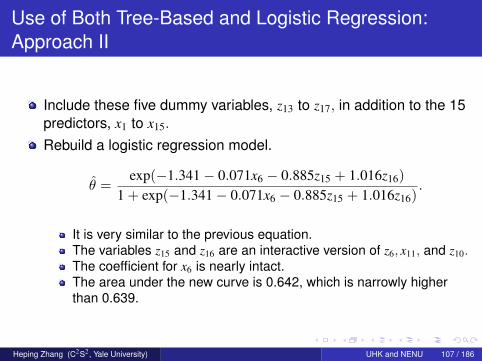
Include these five dummy variables, z13 to z17, in addition to the 15predictors, x1 to x15.
Rebuild a logistic regression model.
θ =exp(−1.341− 0.071x6 − 0.885z15 + 1.016z16)
1 + exp(−1.341− 0.071x6 − 0.885z15 + 1.016z16).
It is very similar to the previous equation.The variables z15 and z16 are an interactive version of z6, x11, and z10.The coefficient for x6 is nearly intact.The area under the new curve is 0.642, which is narrowly higherthan 0.639.
Heping Zhang (C2S2, Yale University) UHK and NENU 107 / 186
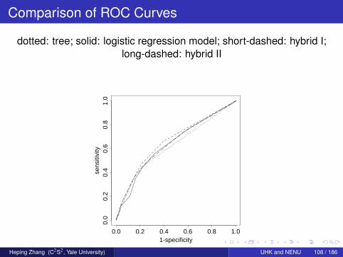
Comparison of ROC Curves
dotted: tree; solid: logistic regression model; short-dashed: hybrid I;long-dashed: hybrid II
1-specificity
sens
itivi
ty
0.0 0.2 0.4 0.6 0.8 1.0
0.0
0.2
0.4
0.6
0.8
1.0
Heping Zhang (C2S2, Yale University) UHK and NENU 108 / 186

Missing Data
Surrogate splits (Breiman et al. 1984, Section 5.3)Imputation (Little and Rubin 1987).Missings Together (Clark and Pregibon 1992)
Heping Zhang (C2S2, Yale University) UHK and NENU 109 / 186

Missing Data
For missings together and imputation, no need to change the treealgorithm.For imputation, missing data can be imputed and entered intotrees as observed.For missings together, we create a new “level” for missing values.
Simple to implement and understand.Easy to trace where the subjects with missing information.
Heping Zhang (C2S2, Yale University) UHK and NENU 110 / 186

Surrogate Splits
Surrogate splits attempt to utilize the information in otherpredictors to assist us in splitting when the splitting variable, say,race, is missing.The idea to look for a predictor that is most similar to race inclassifying the subjects.One measure of similarity between two splits suggested byBreiman et al. (1984) is the coincidence probability that the twosplits send a subject to the same node.
Heping Zhang (C2S2, Yale University) UHK and NENU 111 / 186

Coincidence Probability
The 2× 2 table below compares the split of “is age > 35?” with theselected race split.
Black OthersAge ≤ 35 702 8Age > 35 3017 134
702+134=836 of 3861 subjects are sent to the same node, andhence 836/3861 = 0.217 can be used as an estimate for thecoincidence probability of these two splits.
Heping Zhang (C2S2, Yale University) UHK and NENU 112 / 186

Coincidence Probability
In general, prior information should be incorporated in estimatingthe coincidence probability when the subjects are not randomlydrawn from a general population, such as in case–control studies.We estimate the coincidence probability with
IP{Y = 0}M0(τ)/N0(τ) + IP{Y = 1}M1(τ)/N1(τ),
where Nj(τ) is the total number of class j subjects in node τ andMj(τ) is the number of class j subjects in node τ that are sent tothe same daughters by the two splits; here j = 0 (normal) and1(abnormal). IP{Y = 0} and IP{Y = 1} are the priors to bespecified. Usually, IP{Y = 1} is the prevalence rate of a diseaseunder investigation and IP{Y = 0} = 1− IP{Y = 1}.
Heping Zhang (C2S2, Yale University) UHK and NENU 113 / 186

The Best Surrogate Split
For any split s∗, split s′ is the best surrogate split of s∗ when s′ yieldsthe greatest coincidence probability with s∗ over all allowable splitsbased on different predictors.
Heping Zhang (C2S2, Yale University) UHK and NENU 114 / 186

Surrogate Split
It is possible that the predictor that yields the best surrogate splitmay also be missing.We have to look for the second best, and so on.If our purpose is to build an automatic classification rule (e.g.,Goldman et al., 1982, 1996), it is not difficult for a computer tokeep track of the list of surrogate splits.However, the same task may not be easy for humans.Surrogate splits are rarely published in the literature.
Heping Zhang (C2S2, Yale University) UHK and NENU 115 / 186

Surrogate Split
There is no guarantee that surrogate splits improve the predictivepower of a particular split as compared to a random split. In suchcases, the surrogate splits should be discarded.If surrogate splits are used, the user should take full advantage ofthem. They may provide alternative tree structures that in principlecan have a lower misclassification cost than the final tree,because the final tree is selected in a stepwise manner and is notnecessarily a local optimizer in any sense.
Heping Zhang (C2S2, Yale University) UHK and NENU 116 / 186

Tree Stability
If we take a random sample of 3861 with replacement from theYale Pregnancy Outcome Study, what is the chance that we cometo the same tree as the original one?This chance is not so great, as all stepwise model selectionspotentially suffer from the same problem.While the trees structures are instable, the trees could providevery similar classifications and predictions.
Heping Zhang (C2S2, Yale University) UHK and NENU 117 / 186

Tree for Treatment Effectiveness
In a typical randomized clinical trial, different treatments (say twotreatments) are compared in a study population, and the effectivenessof the treatments is assessed by averaging the effects over thetreatment arms. However, it is possible that the on-average inferiortreatment is superior in some of the patients. The trees provide auseful framework to explore this possibility by identifying patient groupswithin which the treatment effectiveness varies the greatest among thetreatment arms.
Heping Zhang (C2S2, Yale University) UHK and NENU 118 / 186
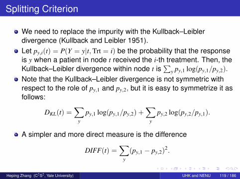
Splitting Criterion
We need to replace the impurity with the Kullback–Leiblerdivergence (Kullback and Leibler 1951).Let py,i(t) = P(Y = y|t,Trt = i) be the probability that the responseis y when a patient in node t received the i-th treatment. Then, theKullback–Leibler divergence within node t is
∑y py,1 log(py,1/py,2).
Note that the Kullback–Leibler divergence is not symmetric withrespect to the role of py,1 and py,2, but it is easy to symmetrize it asfollows:
DKL(t) =∑
y
py,1 log(py,1/py,2) +∑
y
py,2 log(py,2/py,1).
A simpler and more direct measure is the difference
DIFF(t) =∑
y
(py,1 − py,2)2.
Heping Zhang (C2S2, Yale University) UHK and NENU 119 / 186

Splitting Criterion
It is noteworthy that neither DKL nor DIFF is a distance metric andhence does not possess the property of triangle inequality.Consequently, the result does not necessarily improve as we split aparent node into offspring nodes.
Heping Zhang (C2S2, Yale University) UHK and NENU 120 / 186

Limitations of Trees
Tree-based data analyses are readily interpretable.Tree-based methods have their limitations.
Tree structure is prone to instability even with minor dataperturbations.To leverage the richness of a data set of massive size, we need tobroaden the classic statistical view of “one parsimonious model" fora given data set.Due to the adaptive nature of the tree construction, theoreticalinference based on a tree is usually not feasible. Generating moretrees may provide an empirical solution to statistical inference.
Heping Zhang (C2S2, Yale University) UHK and NENU 121 / 186

Random Forests
Forests have emerged as an ideal solution.A forest refers to a constellation of any number of tree models.Such an approach is also referred to as an ensemble.A forest consists of hundreds or thousands of trees, so it is morestable and less prone to prediction errors as a result of dataperturbations (Breiman 1996, 2001).While each individual tree is not a good model, combining theminto a committee improves their value.Trees in a forest should not be pruned; otherwise it would becounterproductive to pool “good" models into a committee.
Heping Zhang (C2S2, Yale University) UHK and NENU 122 / 186

Random Forests
Suppose we have n observations and p predictors.1 Draw a bootstrap sample.2 Apply recursive partitioning to the bootstrap sample. At each
node, randomly select q of the p predictors and restrict the splitsbased on the random subset of the q variables. Here, q should bemuch smaller than p.
3 Let the recursive partitioning run to the end and generate a tree.4 Repeat Steps 1 to 3 to form a forest. The forest-based
classification is made by majority vote from all trees.
Heping Zhang (C2S2, Yale University) UHK and NENU 123 / 186

Random Forests
If Step 2 is skipped, the above algorithm is called bagging(bootstraping and aggregating) (Breiman 1996).Bagging should not be confused with another procedure calledboosting (Freund and Schapire 1996).
One of the boosting algorithms is Adaboost, which makes use oftwo sets of intervening weights.One set, w, weighs the classification error for each observation.The other, β, weighs the voting of the class label.Boosting is an iterative procedure, and at each iteration, a model(e.g., a tree) is built.It begins with an equal w-weight for all observations.Then, the β-weights are computed based on the w-weighted sum oferror, and w-weights are updated with β-weights.With the updated weights, a new model is built and the processcontinues.
Heping Zhang (C2S2, Yale University) UHK and NENU 124 / 186

Forest Size
How many trees do we need in a forest?Because of so many trees in a forest, it is impractical to present aforest or interpret a forest.Zhang and Wang (2009): a tree is removed if its removal from theforest has the minimal impact on the overall prediction accuracy.
Calculate the prediction accuracy of forest F, denoted by pF.For every tree, denoted by T, in forest F, calculate the predictionaccuracy of forest F−T that excludes T, denoted by pF−T .Let ∆−T be the difference in prediction accuracy between F andF−T : ∆−T = pF − pF−T .The tree Tp with the smallest ∆T is the least important one andhence subject to removal: Tp = arg min
T∈F(∆−T).
Heping Zhang (C2S2, Yale University) UHK and NENU 125 / 186

Optimal Size Subforest
Let h(i), i = 1, . . . ,Nf − 1, denote the performance trajectory of asubforest of i trees, where Nf is the size of the original randomforest.If there is only one realization of h(i), they select the optimal sizeiopt of the subforest by maximizing h(i) over i = 1, . . . ,Nf − 1:iopt = arg max
i=1,...,Nf−1(h(i)).
If there are M realizations of h(i), they select the optimal sizesubforest by using the 1-se.
Heping Zhang (C2S2, Yale University) UHK and NENU 126 / 186
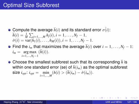
Optimal Size Subforest
Compute the average h(i) and its standard error ˆσ(i):h(i) = 1
M
∑j=1,...,M hj(i), i = 1, . . . ,Nf − 1,
σ(i) = var(h1(i), . . . , hM(i)), i = 1, . . . ,Nf − 1.
Find the im that maximizes the average h(i) over i = 1, . . . ,Nf − 1:im = arg max
i=1,...,Nf−1(h(i)).
Choose the smallest subforest such that its corresponding h iswithin one standard error (se) of h(im) as the optimal subforestsize iopt: iopt = min
i=1,...,M(h(i) > (h(im)− σ(im)).
Heping Zhang (C2S2, Yale University) UHK and NENU 127 / 186

Breast Cancer Prognosis
van de Vijver et al. (2002): the microarray data set of a cohort of295 young patients with breast cancer, containing expressionprofiles from 70 previously selected genes.The responses of all patients are defined by whether the patientsremained disease-free five years after their initial diagnoses or not.To begin the process, an initial forest is constructed using thewhole data set as the training data set.One bootstrap data set is used for execution and the out-of-bag(oob) samples for evaluation.Replicating the bootstrapping procedure 100 times, Zhang andWang (2009) found that the sizes of the optimal subforests fall in arelatively narrow range, of which the 1st quartile, the median, andthe 3rd quartile are 13, 26, and 61, respectively. This allows themto choose the smallest optimal subforest with the size of 7.
Heping Zhang (C2S2, Yale University) UHK and NENU 128 / 186

Comparison of Prediction Performance
Predicted Observed outcomeMethod Error rate outcome Good PoorInitial random forest 26.0% Good 141 17
Poor 53 58Optimal subforest 26.0% Good 146 22
Poor 48 53Published classifier 35.3% Good 103 4
Poor 91 71
Heping Zhang (C2S2, Yale University) UHK and NENU 129 / 186
Importance Score
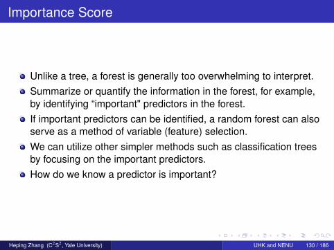
Unlike a tree, a forest is generally too overwhelming to interpret.Summarize or quantify the information in the forest, for example,by identifying “important" predictors in the forest.If important predictors can be identified, a random forest can alsoserve as a method of variable (feature) selection.We can utilize other simpler methods such as classification treesby focusing on the important predictors.How do we know a predictor is important?
Heping Zhang (C2S2, Yale University) UHK and NENU 130 / 186
Gini Importance
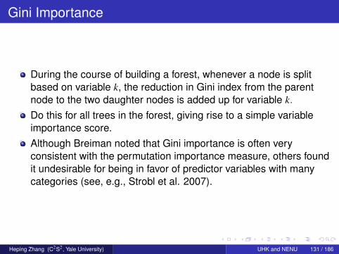
During the course of building a forest, whenever a node is splitbased on variable k, the reduction in Gini index from the parentnode to the two daughter nodes is added up for variable k.
Do this for all trees in the forest, giving rise to a simple variableimportance score.Although Breiman noted that Gini importance is often veryconsistent with the permutation importance measure, others foundit undesirable for being in favor of predictor variables with manycategories (see, e.g., Strobl et al. 2007).
Heping Zhang (C2S2, Yale University) UHK and NENU 131 / 186

Depth Importance
Chen et al. (2007) introduced an importance index that is similarto Gini importance score, but considers the location of the splittingvariable as well as its impact.Whenever node t is split based on variable k, let L(t) be the depthof the node and S(k, t) be the χ2 test statistic from the variable,then 2−L(t)S(k, t) is added up for variable k over all trees in theforest.The depth is 1 for the root node, 2 for the offspring of the rootnode, and so forth.This depth importance measure was found useful in identifyinggenetic variants for complex diseases, although it is not clearwhether it also suffers from the same end-cut preference problem.
Heping Zhang (C2S2, Yale University) UHK and NENU 132 / 186

Permutation Importance
Also referred to as the variable importance.For each tree in the forest, we count the number of votes cast forthe correct class.We randomly permute the values of variable k in the oob casesand recount the number of votes cast for the correct class in theoob cases with the permuted values of variable k.Average the differences between the number of votes for thecorrect class in the variable-k-permuted oob data from the numberof votes for the correct class in the original oob data, over all treesin the forest.
Heping Zhang (C2S2, Yale University) UHK and NENU 133 / 186

Permutation Importance
Arguably the most commonly used choice.Not necessarily positive, and does not have an upper limit.Both the magnitudes and relative rankings of the permutationimportance for predictors can be unstable when the number, p, ofpredictors is large relative to the sample size.The magnitudes and relative rankings of the permutationimportance for predictors vary according to the number of trees inthe forest and the number, q, of variables that are randomlyselected to split a node.
Heping Zhang (C2S2, Yale University) UHK and NENU 134 / 186

Permutation Importance
111
1 1 1 1 1 1 1 1 1
0 500 1000 1500 2000
02
46
810
12
222 2 2 2 2 2 2 2 2 2
33 3 3 3 3 3 3 3 3 3 344
4
4
44
44
4 4 4 4
Heping Zhang (C2S2, Yale University) UHK and NENU 135 / 186

Permutation Importance
there are conflicting numerical reports with regard to thepossibility that the permutation importance overestimates thevariable importance of highly correlated variables.Genuer et al. (2008): specifically addressed this issue withsimulation studies and concluded that the magnitude of theimportance for a predictor steadily decreases when more variableshighly correlated with the predictor are included in the data set.
Heping Zhang (C2S2, Yale University) UHK and NENU 136 / 186

Permutation Importance
Began with the four selected genes.Identified the genes whose correlations with any of the fourselected genes are at least 0.4.Those correlated genes are divided randomly in five sets of aboutsame size.We added one, two, . . . , and five sets of them sequentiallytogether with the four selected genes as the predictors.
Heping Zhang (C2S2, Yale University) UHK and NENU 137 / 186

Permutation Importance
The x-axis is the number of correlated sets of genes and they-axis the importance score.The forest size is set at 1000.q equals the square root of the forest size for the left panel and 8for the right panel.The rankings of the predictors are preserved.
11 1 1 1
1 2 3 4 5
02
46
810
12
22 2 2 2
33 3 3 3
4
4
4
4
41
11
1 1
1 2 3 4 5
05
1015
2 2 2 2 23
33 3 3
4
4
4
44
Heping Zhang (C2S2, Yale University) UHK and NENU 138 / 186

Permutation Importance
Included genes that are correlated with any of the correlated geneat least 0.6, 0.4, and 0.2.The ranking is more relevant than the magnitude
1 1 1
1
01
23
45
N 0.2 0.4 0.6
2 2 2
2
3 3 3
3
4 44
4
1 1 1
1
01
23
45
N 0.2 0.4 0.6
2 2 2
2
3 3 3
3
4 44
4
Heping Zhang (C2S2, Yale University) UHK and NENU 139 / 186

Maximum Conditional Importance
Wang et al. (2010): introduced a maximal conditional chi-square(MCC) importance by taking the maximum chi-square statisticresulting from all splits in the forest that use the same predictor.MCC can distinguish causal predictors from noise.MCC can assess interactions.
Consider the interaction between two predictors xi and xj.For xi, suppose its MCC is reached in node ti of a tree within aforest. Whenever xj splits an ancestor of node ti, we count one andotherwise zero.The final frequency, f , can give us a measure of interactionbetween xi and xj.Through the replication of the forest construction we can estimatethe frequency and its precision.
Heping Zhang (C2S2, Yale University) UHK and NENU 140 / 186

Maximum Conditional Importance
They generated 100 predictors independently, each of them is thesum of two i.i.d. binary variables (0 or 1).For the first 16 predictors, the underlying binary random variablehas the success probability of 0.282.For the remaining 84, they draw a random number between 0.01and 0.99 as the success probability of the underlying binaryrandom variable.The first 16 predictors serve as the risk variables and theremaining 84 the noise variables.
Heping Zhang (C2S2, Yale University) UHK and NENU 141 / 186

Maximum Conditional Importance
The outcome variable is generated as follows.The 16 risk variables are divided equally into four groups, andwithout loss of generality, say sequentially.Once these 16 risk variables are generated, we calculate thefollowing probability on the basis of which the response variable isgenerated: w = 1−Π(1−Πqk) where the first product is withrespect to the four groups, the second product is with respect tothe first predictors inside each group, and q0 = 1.2× 10⁻⁸,q1 = 0.79, and q2 = 1. The subscript k equals the randomlygenerated value of the respective predictor.
Heping Zhang (C2S2, Yale University) UHK and NENU 142 / 186

Maximum Conditional Importance
Generate the first 200 possible controls and the first 200 possiblecases.This completes the generation of one data set.Replicate the entire process 1000 times.
Heping Zhang (C2S2, Yale University) UHK and NENU 143 / 186

Interaction Heat Map
>16
16
15
14
13
12
11
10
9
8
7
6
5
4
3
2
1
1 2 3 4 5 6 7 8 9 10 11 12 13 14 15 160.00
0.05
0.10
0.15
0.20
0.25
0.30
0.35
0.40
The x-axis is the sequence number of the primary predictor and they-axis the sequence number of the potential interacting predictor. The
intensity expresses the frequency when the potential interactingpredictor precedes the primary predictor in a forest.
Heping Zhang (C2S2, Yale University) UHK and NENU 144 / 186

Impact on MCC by Correlated Predictors
1 1 11
1
1 2 3 4 5
020
4060
80
2 2 2 2 23
3 3 3 3
4 4 4 4 4
1 1 1 1 1
1 2 3 4 50
2040
6080
2 2 2 2 23 3 3 3 3
4 4 4 4 4
Heping Zhang (C2S2, Yale University) UHK and NENU 145 / 186
Predictors with Uncertainties
In general, we base our analysis on predictors that are observedwith certainty.However, this is not always the case.
To identify genetic variants for complex diseases, haplotypes aresometimes the predictors.A haplotype is a combination of single nucleotidepolymorphisms(SNPs) on a chromatid.Has to be statistically inferred from the SNPs in frequencies.
Heping Zhang (C2S2, Yale University) UHK and NENU 146 / 186

Predictors with Uncertainties
We assume x1 is the only categorical variable with uncertainties,and it has K possible levels.For the i-th subject, xi1 = k with a probability pik (
∑Kk=1 pik = 1).
To identify genetic variants for complex diseases, haplotypes aresometimes the predictors.A haplotype is a combination of single nucleotidepolymorphisms(SNPs) on a chromatid.Has to be statistically inferred from the SNPs in frequencies.
Heping Zhang (C2S2, Yale University) UHK and NENU 147 / 186

Predictors with Uncertainties
In a typical random forest, the “working" data set is a bootstrapsample of the original data set.Here, a “working" data set is generated according to thefrequencies of x1 while keeping the other variables intact.the data set would be {zi1, xi2, . . . , xip, yi}n
i=1, where zi1 is randomlychosen from 1, . . . ,K, according to the probabilities (pi1, . . . , piK).
Once the data set is generated, the rest can be carried out in thesame way as for a typical random forest.
Heping Zhang (C2S2, Yale University) UHK and NENU 148 / 186

Predictors with Uncertainties
unphaseddata
?frequenciesestimated
�������
�
@@R
phaseddata set 1
-
phaseddata set 2
-
...
phaseddata set B
-
-JJJ
BBBBBBBN
tree 1
-�
BBBBBBN
tree 2
...
-������
���������
tree B
importancefor x1
importancefor x2
...
importancefor xp
Heping Zhang (C2S2, Yale University) UHK and NENU 149 / 186

Notation
Let δ indicate whether a subject’s survival is observed (one if it is)or censored (zero if it is not).Let Y denote the observed time.In the absence of censoring, the observed time is the survivaltime, and hence Y = T.
Otherwise, the observed time is the censoring time, denoted by U.
Y = min(T,U) and δ = I(Y = T), where I(·) is an indicator function.
Heping Zhang (C2S2, Yale University) UHK and NENU 150 / 186

Data Example
Smoked Time (days) Smoked Time Smoked Timeyes 11906+ yes 9389+ yes 4539+yes 11343+ yes 9515+ yes 10048+yes 5161 yes 9169 no 8147+yes 11531+ yes 11403+ yes 11857+yes 11693+ no 10587 yes 9343+yes 11293+ yes 6351+ yes 502+yes 7792 no 11655+ yes 9491+yes 2482+ no 10773+ yes 11594+no 7559+ yes 11355+ yes 2397
yes 2569+ yes 2334+ yes 11497+yes 4882+ yes 9276 yes 703+yes 10054 no 11875+ no 9946+yes 11466+ no 10244+ yes 11529+yes 8757+ no 11467+ yes 4818yes 7790 yes 11727+ no 9552+yes 11626+ yes 7887+ yes 11595+yes 7677+ yes 11503 yes 10396+yes 6444+ yes 7671+ yes 10529+yes 11684+ yes 11355+ yes 11334+yes 10850+ yes 6092 yes 11236+
Heping Zhang (C2S2, Yale University) UHK and NENU 151 / 186
Survival and Hazard Function
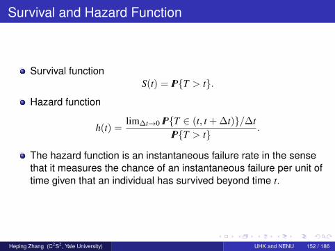
Survival functionS(t) = IP{T > t}.
Hazard function
h(t) =lim∆t→0 IP{T ∈ (t, t + ∆t)}/∆t
IP{T > t}.
The hazard function is an instantaneous failure rate in the sensethat it measures the chance of an instantaneous failure per unit oftime given that an individual has survived beyond time t.
Heping Zhang (C2S2, Yale University) UHK and NENU 152 / 186

Estimate Survival Function
Parametric Approach: distributions of survival can be assumed.Exponential: S(t) = exp(−λt) (λ > 0), where λ is an unknownconstant.Only need to estimate the constant hazard.The full likelihood function
L(λ) =
60∏i=1
[λ exp(−λTi)]δi [exp(−λUi)]
1−δi .
Heping Zhang (C2S2, Yale University) UHK and NENU 153 / 186

Estimate Survival Function
For the sample data, the log likelihood function
l(λ) =
60∑i=1
{δi[log(λ)− λYi]− λ(1− δi)Yi}
= log(λ)
60∑i=1
δi − λ60∑
i=1
Ti
= 11 log(λ)− λ(11906 + 11343 + · · ·+ 11236),
where 11 is the number of uncensored survival times and thesummation is over all observed times.The maximum likelihood estimate of the hazard, λ, isλ = 11
527240 = 2.05/105, which is the number of failures divided bythe total observed time.
Heping Zhang (C2S2, Yale University) UHK and NENU 154 / 186
Validate Survival Function
Compare a parametric fit with the nonparametric Kaplan–MeierCurve.Plot the empirical cumulative hazard function against the assumedtheoretical cumulative hazard function at times when failuresoccurred.
The cumulative hazard function is defined as H(t) =∫ t
0 h(u)du.
Heping Zhang (C2S2, Yale University) UHK and NENU 155 / 186

Exponential and Kaplan–Meier Curves
time
surv
ival
0 2000 4000 6000 8000 10000 12000
0.70
0.75
0.80
0.85
0.90
0.95
1.00
Heping Zhang (C2S2, Yale University) UHK and NENU 156 / 186

Cumulative Hazard Functions
Survival Risk set Failures Hazard rate Cumulative hazardtime K d d/K Empirical Assumed
2397 57 1 0.0175 0.0175 0.04914818 53 1 0.0189 0.0364 0.09885161 51 1 0.0196 0.0560 0.10586092 50 1 0.0200 0.0760 0.12497790 44 1 0.0227 0.0987 0.15977792 43 1 0.0233 0.1220 0.15979169 39 1 0.0256 0.1476 0.18809276 38 1 0.0263 0.1740 0.1902
10054 30 1 0.0333 0.2073 0.206110587 26 1 0.0385 0.2458 0.217011503 13 1 0.0769 0.3227 0.2358
Heping Zhang (C2S2, Yale University) UHK and NENU 157 / 186

Product Limit Estimate of Survival Function
Survival Risk set Failures Ratio Producttime K d (K − d)/K S(t)
2397 57 1 0.982 0.9824818 53 1 0.981 0.982 ∗ 0.981 = 0.9635161 51 1 0.980 0.963 ∗ 0.980 = 0.9446092 50 1 0.980 0.944 ∗ 0.980 = 0.9257790 44 1 0.977 0.925 ∗ 0.977 = 0.9047792 43 1 0.977 0.904 ∗ 0.977 = 0.8839169 39 1 0.974 0.883 ∗ 0.974 = 0.8609276 38 1 0.974 0.860 ∗ 0.974 = 0.838
10054 30 1 0.967 0.838 ∗ 0.967 = 0.81010587 26 1 0.962 0.810 ∗ 0.962 = 0.77911503 13 1 0.923 0.779 ∗ 0.923 = 0.719
Heping Zhang (C2S2, Yale University) UHK and NENU 158 / 186
Cumulative Hazard vs Kaplan–Meier Curve
The mechanism of producing the Kaplan–Meier curve is similar tothe generation of the empirical cumulative hazard function.The first three columns are the same.The fourth columns differ by one, namely, the proportion ofindividuals who survived beyond the given time point.
Heping Zhang (C2S2, Yale University) UHK and NENU 159 / 186

Log-Rank Test
In many clinical studies, a common goal is to compare the survivaldistributions of various groups.
Time
Sur
viva
l
0 2000 4000 6000 8000 10000 12000
0.70
0.75
0.80
0.85
0.90
0.95
1.00
Heping Zhang (C2S2, Yale University) UHK and NENU 160 / 186

Log-Rank Test
Peto and Peto (1972): at the distinct failure times, we have a sequence
of 2× 2 tables.
Dead AliveSmoking ai ni
Nonsmokingdi Ki
Time Risk set FailuresTi Ki di ai ni Ei Vi
2397 57 1 1 47 0.825 0.1454818 53 1 1 43 0.811 0.1535161 51 1 1 41 0.804 0.1586092 50 1 1 40 0.800 0.1607790 44 1 1 35 0.795 0.1637792 43 1 1 34 0.791 0.1659169 39 1 1 31 0.795 0.1639276 38 1 1 30 0.789 0.166
10054 30 1 1 24 0.800 0.16010587 26 1 0 21 0.808 0.15511503 13 1 1 11 0.846 0.130
The log-rank test statistic is LR =∑k
i=1(ai−Ei)√∑ki=1 Vi
, where k is the number of
distinct failure times, Ei = diniKi, and Vi =
(di(Ki−ni)niKi(Ki−1)
)(1− di
Ki
).
Heping Zhang (C2S2, Yale University) UHK and NENU 161 / 186

Log-Rank Test
Time Risk set FailuresTi Ki di ai ni Ei Vi
2397 57 1 1 47 0.825 0.1454818 53 1 1 43 0.811 0.1535161 51 1 1 41 0.804 0.1586092 50 1 1 40 0.800 0.1607790 44 1 1 35 0.795 0.1637792 43 1 1 34 0.791 0.1659169 39 1 1 31 0.795 0.1639276 38 1 1 30 0.789 0.166
10054 30 1 1 24 0.800 0.16010587 26 1 0 21 0.808 0.15511503 13 1 1 11 0.846 0.130
The log-rank test statistic has an asymptotic standard normaldistribution, we test the hypothesis that the two survival functionsare the same by comparing LR with the quantiles of the standardnormal distribution.For our data, LR = 0.87, corresponding to a two-sided p-value of0.38.
Heping Zhang (C2S2, Yale University) UHK and NENU 162 / 186
Cox Proportional Hazard Regression
Instead of making assumptions directly on the survival times, Cox(1972) proposed to specify the hazard function.Suppose that we have a set of predictors x = (x1, . . . , xp).
The Cox proportional hazard model is
λ(t; x) = exp(xβ)λ0(t),
where β is a p× 1 vector of unknown parameters and λ0(t) is anunknown function giving a baseline hazard for x = 0.
Heping Zhang (C2S2, Yale University) UHK and NENU 163 / 186

Cox Proportional Hazard Regression
If we take two individuals i and j with covariates xi and xj, the ratioof their hazard functions is exp((xi − xj)β), which is free of time.The hazard functions for any two individuals are parallel in time.λ0(t) is left to be arbitrary. Thus, the proportional hazard can beregarded as semiparametric.
Heping Zhang (C2S2, Yale University) UHK and NENU 164 / 186

Conditional Likelihood
Condition the likelihood on the set of uncensored times.At any time t, let R(t) be the risk set, i.e., the individuals who wereat risk right before time t. For each uncensored time Ti, the hazardrate is h(Ti) = IP{A death in (Ti,Ti + dt) | R(Ti)}/dt.
Under the proportional hazard model,
IP{A death in (Ti,Ti + dt) | R(Ti)} = exp(xβ)λ0(Ti)dt
and
IP{Individual i fails at Ti | one death in R(Ti) at time Ti}
=exp(xiβ)∑
j∈R(Ti)exp(xjβ)
.
Heping Zhang (C2S2, Yale University) UHK and NENU 165 / 186

Conditional Likelihood
The entire conditional likelihood is the product of those by failedindividual i
L(β) =∏
failure i
exp(xiβ)∑j∈R(Ti)
exp(xjβ).
Maximizing the conditional likelihood gives rise to the estimates ofβ.
β has an asymptotic normal distribution.
Heping Zhang (C2S2, Yale University) UHK and NENU 166 / 186

The Western Collaborative Group Study
A prospective and long-term study of coronary heart disease.In 1960–61, 3154 middle-aged white males from ten largeCalifornia corporations in the San Francisco Bay Area and LosAngeles entered the WCGS, and they were free of coronary heartdisease and cancer.After a 33-year follow-up, 417 of 1329 deaths were due to cancerand 43 were lost to follow-up.
Heping Zhang (C2S2, Yale University) UHK and NENU 167 / 186
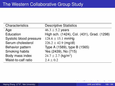
The Western Collaborative Group Study
Characteristics Descriptive StatisticsAge 46.3± 5.2 yearsEducation High sch. (1424), Col. (431), Grad. (1298)Systolic blood pressure 128.6± 15.1 mmHgSerum cholesterol 226.2± 42.9 (mg/dl)Behavior pattern Type A (1589), type B (1565)Smoking habits Yes (2439), No (715)Body mass index 24.7± 2.7 (kg/m2)Waist-to-calf ratio 2.4± 0.2
Heping Zhang (C2S2, Yale University) UHK and NENU 168 / 186
The Western Collaborative Group Study
We entered the eight predictors into an initial Cox’s model andused a backward stepwise procedure to delete the least significantvariable from the model at the threshold of 0.05.coxph(Surv(time, cancer) age + chol + smoke +wcr).
Heping Zhang (C2S2, Yale University) UHK and NENU 169 / 186

Parameter Estimation for Cox’s Model
Variable Coefficient S.E. p-valueAge (age) 0.0934 0.009 0.000Serum cholesterol (chol) 0.0026 0.001 0.033Smoking habits (smoke) 0.2263 0.103 0.029Waist-to-calf ratio (wcr) 0.7395 0.271 0.006
Heping Zhang (C2S2, Yale University) UHK and NENU 170 / 186
Assessing Proportionality
Dichotomize age, serum cholesterol, and waist-to-calf ratio at theirmedian levels.The 2882 (= 3154− 272) subjects are divided into 16 cohortsWithin each cohort i, we calculate the Kaplan–Meier survivalestimate Si(t).
Plot log(− log(Si(t))) versus time as shown in Figure ??.
Heping Zhang (C2S2, Yale University) UHK and NENU 171 / 186

Assessing Proportionality
time
log(
-log(
surv
ival
))
2000 4000 6000 8000 10000 12000
-5-4
-3-2
-1
time
log(
-log(
surv
ival
))
2000 4000 6000 8000 10000 12000
-5-4
-3-2
-1
time
log(
-log(
surv
ival
))
2000 4000 6000 8000 10000 12000
-5-4
-3-2
-1
time
log(
-log(
surv
ival
))
2000 4000 6000 8000 10000 12000
-5-4
-3-2
-1
Heping Zhang (C2S2, Yale University) UHK and NENU 172 / 186

Assessing Proportionality
h(t) = − d log(S(t))dt , which is equivalent to S(t) = exp
(−∫ t
0 h(z)dz).
The survival function is
S(t; x) = exp[−∫ t
0exp(xβ)λ0(z)
]= exp
[− exp(xβ)
∫ t
0λ0(z)
]. (1)
log(− log[S(t; x)]) = xβ + log[∫ t
0 λ0(z)].
The log-log survival curves in our 16 cohorts are supposed to beparallel if the proportional hazard assumption holds.
Heping Zhang (C2S2, Yale University) UHK and NENU 173 / 186

Gordon and Olshen’s Rule
Gordon and Olshen (1985): What would be an appropriatemeasure of node impurity in the context of censored data?We would regard a node as pure if all failures in the node occurredat the same time.
1 1 1
0 0 0time time time
(a) (b) (c)
Heping Zhang (C2S2, Yale University) UHK and NENU 174 / 186

Gordon and Olshen’s Rule
How far the within-node Kaplan–Meier curve deviates from any ofthe curves in P.Need first to define a distance between the two Kaplan–Meiercurves.
Lp Wasserstein metrics[∫ 1
0 |F−11 (u)− F−1
2 (u)|pdu]1/p
, where
F−1i (u) = min{t : Fi(t) ≥ u}, i = 1, 2.
Heping Zhang (C2S2, Yale University) UHK and NENU 175 / 186
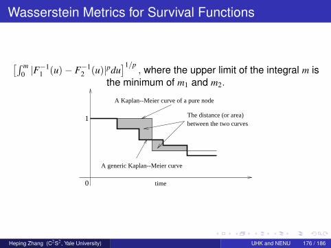
Wasserstein Metrics for Survival Functions
[∫ m0 |F
−11 (u)− F−1
2 (u)|pdu]1/p
, where the upper limit of the integral m isthe minimum of m1 and m2.
1
0 time
A Kaplan--Meier curve of a pure node
A generic Kaplan--Meier curve
The distance (or area)between the two curves
Heping Zhang (C2S2, Yale University) UHK and NENU 176 / 186

Node Impurity
i(τ) = minδS∈P dp(Sτ , δS), where Sτ is the Kaplan–Meier curvewithin node τ, and the minimization minδS∈P means that Sτ iscompared with its best match among the three curves.When p = 1, this can be viewed as the deviation of survival timestoward their median.When p = 2, it corresponds to the variance of the Kaplan–Meierdistribution estimate of survival.With this node impurity, we can grow a survival tree.
Heping Zhang (C2S2, Yale University) UHK and NENU 177 / 186

Maximizing the Difference
When two daughter nodes are relatively pure, they tend to differfrom each other.Finding two different daughters is a means to increase thebetween variation and consequently to reduce the within variation.Select a split that maximizes the “difference” between the twodaughter nodes, or, equivalently, minimizes their similarity.Ciampi et al. (1986) and Segal (1988): The log-rank test is acommonly used approach for testing the significance of thedifference between the survival times of two groups.
Heping Zhang (C2S2, Yale University) UHK and NENU 178 / 186

Likelihood Functions
Davis and Anderson (1989): assume that the survival functionwithin any given node is an exponential function with a constanthazard.LeBlanc and Crowley (1992) and Ciampi et al. (1995): the hazardfunctions in two daughter nodes are proportional (the full or partiallikelihood function can be used).All individuals in node τ have the hazard λτ (t) = θτλ0(t), whereλ0(t) is the baseline hazard independent of the node and θτ is anonnegative parameter corresponding to exp(xβ).Treat the value of the “covariate" as the same inside eachdaughter node, hence exp(xβ) becomes a single parameter θτ .
Heping Zhang (C2S2, Yale University) UHK and NENU 179 / 186

Likelihood Functions
The survival function of individuals in node τ isS(t; τ) = exp[−θτΛ0(t)], where Λ0(t) is the baseline cumulativehazard function integrated from λ0(t).
The full likelihood function within node τ asL(θτ , λ0) =
∏{i∈ node τ}[λ0(Ti)θτ ]δi exp[−Λ0(Ui)θτ ].
The full likelihood of the entire learning sample for a tree T can beexpressed as L(θ, λ0; T ) =
∏τ∈T L(θτ , λ0), which is the product of
the full likelihoods contributed by all terminal nodes of T .
Heping Zhang (C2S2, Yale University) UHK and NENU 180 / 186
Likelihood Functions
Every time we partition a node into two, we need to maximize thefull tree likelihood.Too ambitious for computation; e.g., the cumulative hazard Λ0 isunknown and must be estimated over and over again.As a remedy, LeBlanc and Crowley propose to use a one-step
Breslow’s (1972) estimate Λ0(t) =
∑i:Yi≤t δi
|R(t)| , where the denominator|R(t)| is the number of subjects at risk at time t.
The one-step estimate of θτ is then θτ =∑{i∈ node τ} δi∑
{i∈ node τ} Λ0(Yi), which
can be interpreted as the number of failures divided by theexpected number of failures in node τ under the assumption of nostructure in survival times.
Heping Zhang (C2S2, Yale University) UHK and NENU 181 / 186

A Straightforward Extension
Zhang (1995): we observe a binary death indicator, δ, and theobserved time.Treat them as two outcomes, we can compute the within-nodeimpurity, iδ, of the death indicator and the within-node quadraticloss function, iy, of the time.Combine wδiδ + wyiy.
Heping Zhang (C2S2, Yale University) UHK and NENU 182 / 186

Pruning a Survival Tree
Using any of the splitting criteria above, we can produce an initialtree.How do we prune the initial survival tree, T ?Cost-complexity Rα(T ) = R(T ) + α|T |, where R(T ) is the sum ofthe costs over all terminal nodes of T .
Heping Zhang (C2S2, Yale University) UHK and NENU 183 / 186

Random Survival Forests
Once we are able to construct a survival tree, we can use thesame method described above to construct a random survivalforest (Ishwaran et al. 2008).
Heping Zhang (C2S2, Yale University) UHK and NENU 184 / 186

Survival Trees for the Western Collaborative GroupStudy
11.68.6 20.8
25.5
129.4
11.9
4.1
4.77.26.57.910.7
3.2 8.6 9.3 13.1 22.9 7.7
10.7
9.3 7.7
4.7
10.7
25.5
129.4
11.9
4.7
11.6
7.722.913.18.63.2
7.2
9.3
13.322.9
22.9
An initial large tree obtained by the log-rank testing statistic. The topand bottom numbers under the node are respectively the original and
maximized values of the statistic.
Heping Zhang (C2S2, Yale University) UHK and NENU 185 / 186

Maximum Log-rank Statistic vs. Tree Size
•••••••••
••
•
tree size
logr
ank
stat
istic
10 20 30 40
020
4060
8010
012
0
Heping Zhang (C2S2, Yale University) UHK and NENU 186 / 186
Related Documents