Recursive Estimation of Dynamic Models Using Cook's Distance, With Application to Wind Energy Forecast

Working Paper 02-55 (15)

Statistics and Econometrics Series

November 2002

Departamento de Estadística y Econometría

Universidad Carlos III de Madrid

Calle Madrid, 126

28903 Getafe (Spain)

Fax (34) 91 624-98-49

RECURSIVE ESTIMATION OF DYNAMIC MODELS USING COOK'SDISTANCE, WITH APPLICATION TOWIND ENERGY FORECAST

Ismael Sánchez*

AbstractThis article proposes an adaptive forgetting factor for the recursive estimation of time

varying models. The proposed procedure is based on the Cook's distance of the new

observation. It is proven that the proposed procedure encompasses the adaptive features of

classic adaptive forgetting factors and, therefore, has a larger adaptability than its

competitors. The proposed forgetting factor is applied to wind energy forecast, showing

advantages with respect to alternative procedures.

Keywords: Adaptive forgetting factors; Dynamic models; Recursive least squares; Windenergy forecasting.

*Sánchez, Departmento de Estadística y Econometría; Universidad Carlos III de Madrid;Avd. de la Universidad 30, 28911, Leganés, Madrid (Spain). email: [email protected]. This research was supported in part by CICYT, grant BEC2000-0167 and RedEléctrica de España.

1 Introduction

1.1 General considerations

In many applications, the relationship between the variables involved in a forecasting model changes with the

time. Several factors can help to explain this behavior, such as omitted variables, functional misspecifications,

irregular external interventions, and so forth. In this setting, a forecasting system that assumes constant

parameters will lose efficiency, and an adaptive forecasting system will be more appropriate. One of the key

steps for building an adaptive forecasting system is the recursive estimation of the time-varying parameters.

The recursive estimation is also denoted as on-line estimation or adaptive estimation, and in the engineering

literature it is traditionally referred to as recursive identification.

When the parameters of the predictor follow some identified model, the Kalman filter constitutes a convenient

framework to efficiently update the parameter estimates. In this article, however, we are interested in procedures

that do not assume specific laws of parameter evolution. These procedures will be especially useful in highly non-

linear systems, in stand-alone applications, or as initial exploratory tool to identify a model for the parameter

variation to further apply, for instance, Kalman filter. A popular adaptive estimation method that belongs to

this kind of procedures is the recursive least squares (RLS) method. The tracking capability of RLS comes

from the exponentially decreasing weight of older observations into the objective function. As a result, when

computing the parameter estimates, the more recent data is more informative than the old data. As remarked

in Grillenzoni (1994), RLS is considered a more flexible and adaptive procedure than some alternative methods.

This relative superiority has made RLS a widespread procedure in many fields that range from the chemical

industry to economics.

The main element in RLS is the so-called forgetting factor, used to down-weight the past data points.

Typically, the choice of the forgetting factor is a compromise between the ability to track changes in the

parameters and the need to reduce the variance of the prediction error. Putting excessive weight in recent

observations will guarantee fast parameter tracking but, however, at the expense of unnecessarily high variability.

The choice of the forgetting factor has, therefore, a substantial effect on the estimated parameters and in the

efficiency of the predictions. In spite of this sensitivity, the literature about efficient selection of forgetting

factors is scarce, and mainly devoted to the selection of constant forgetting factors (Ljung and Söderström ,1983;

Grillenzoni, 1994). However, the need for an adaptive forgetting factor can be apparent in many applications.

2

For instance, the system can evolve slowly for some period, have quick changes in some other period, or even

remain stationary for a period of time. The uncertainty about the future behavior of a non-linear system can,

then, make advisable to use an adaptive forgetting factor.

There has been a number of approaches in the literature that address the problem of constructing an adaptive

forgetting factor (see, e.g. Fortescue et al., 1981; Goodwin and Sin, 1984, p. 227; Landau et al., 1998, p. 63;

Grillenzoni, 2000). A common feature of those approaches is their ad hoc nature, often based on arbitrary scaling

factors. This article proposes a procedure to obtain an adaptive forgetting factor based on statistical arguments.

The proposed procedure is based on the link between the influence of a new observation and the probability that

the parameters have changed in that period. Usually, the goal of measuring influence and detecting outlying

observations is to avoid such influence in the model. When building an adaptive model, we would also benefit

from measuring the influence of the new observation, but now the goal is it to ease the incorporation of the new

information into the adaptive model. In this article, the influence of the new observation is measured through

Cook’s distance (Cook, 1977).

The article is organized as follows: Section 2 discusses time varying parameter estimation using RLS. Section

3 proposes a class of forgetting factors based on Cook’s distance. Finally, Section 4 illustrates the advantage of

the proposed procedure with simulated and real data related with wind energy forecast.

1.2 Wind energy data

The motivation for the present research was the construction of an efficient forecasting system for wind energy

forecast. Wind energy has become a promising energy source. It has not only an economic interest but it is also

a key element in order to replace fossil energy with sustainable energy resources. Wind energy has, however, the

disadvantage of not being dispatchable. Therefore, accurate forecasting of the wind power up to two days ahead

is recognized as a major contribution for reliable large-scale wind power integration. In a liberalized electricity

market, such a forecasting ability will help to enhance the position of wind energy compared to other forms of

dispatchable energy.

From the statistical point of view, wind energy data has some interesting features that can be summarized

as follows: (i) the relationship between the velocity of the wind and the generated power is highly nonlinear

and, therefore, candidate predictors have the risk of only being reliable in certain range of data; and (ii) this

relationship is time varying because it depends on other variables as wind direction, local air density, local

3

0 5 10 15 20 250

0.5

1

1.5

2

2.5

3

3.5x 104 (a)

Velocity of wind

Out

put p

ower

Period 1Period 2

0 2 4 6 8 10 12 14 16 18 200

0.5

1

1.5

2

2.5

3

3.5x 104 (b)

Velocity of wind

Out

put p

ower

Period 1Period 2

Figure 1: Hourly average wind speed and generated power in a wind farm in Spain. In

each picture, Periods 1 and 2 are consecutive.

temperature variations, local effects of clouds and rain, and so forth. Since some of these variables are difficult

to foresee or even to measure, they can not appropriately be included into a model. Consequently, when building

a forecasting model that predicts output power using the velocity of the wind as input, a constant parameter

model is not satisfactory. Figure 1 shows some typical situations on wind energy data that help to understand

the usefulness of a time varying predictor. In this figure, both pictures (a) and (b) show 200 consecutive hourly

points of velocity of wind (hourly average) and generated power in certain wind farm in Spain. The first 100

points are marked with a circle (o), whereas the last 100 points are marked with the plus sign (+). It can be

seen in these pictures that a model fitted using the first 100 points (Period 1) will produce a poor performance

when applied to the next 100 points (Period 2).

In picture (a), it seems that very different models will be needed in Periods 1 and 2. In Period 1, the

relationship between wind and power seems to follow a quadratic or cubic polynomial with positive first and

second derivatives. However, in the next 100 points, the situation changes. A possible explanation of this

behavior is that, due to the strong wind, a limit in the output has been reached, and the automatic control

system of the windmills has provoked a negative relationship between the variables in order to avoid damages

in the mechanical and electrical parts. In picture (b), the model fitted in Period 1 will underestimate the

performance of the wind farm in period 2. It is very likely that these data points share the same parametric

model but with slightly different parameter values. This can be produced by changes in wind direction or other

meteorological changes. In both examples, an adaptive forecasting system will likely yield better performance

4

than a predictor based on constant parameters.

2 Analysis of RLS with time varying parameters

2.1 A recursive algorithm for a time varying transfer function

This section introduces RLS applied to a general dynamic model. This description will allow to settle the

notation and to illustrate the leading role of the forgetting factor into the recursion. A dynamic model can be

written in several forms. Since we are interested in building a predictor, a useful notation to define the time

series yt is the following dynamic regression:

φt(B)yt = x0tαt + θt(B)at, (1)

where at is a sequence of iid random variable with zero expectation and E(at) = σ2 < ∞. The vector x0t =

(x1t, ..., xkt) is a set of exogenous explanatory variables that can be either deterministic or stochastic. The

polynomials on the shift operator φt(B) = 1 − φ1tB − · · · − φptBp and θt(B) = 1 − θ1tB − · · · − θqtBq have

roots whose realizations entirely lie outside the unit circle, with the exception, at most, of finite sets of points

(Grillenzoni, 2000). For convenience, this model can be written as

yt = z0tβt + at, (2)

with β0t = (φ1t, ..., φpt, α1t, ..., αkt,−θ1, ...,−θq) and z0t = (yt−1, ..., yt−p, x1t, ..., xkt, at−1, ..., at−q). The vector ztcan be interpreted as the input variables, and yt as the output. The RLS estimator for the parameter vector

βt is (Ljung and Söderström, 1983)

βt = βt−1 + Γtξtat, (3)

with at = yt − z0tβt−1 being the one-step ahead prediction error, where z0t = (yt−1, ..., yt−p, x1t, ... , xkt,

at−1, ..., at−q) and where

ξt = −∂at(βt)

∂βt

¯βt=βt−1

. (4)

To obtain this gradient, we can write, using (1), that at = θ−1t (B)φt(B)yt−θ−1t (B)x0tαt. Then, it can be checked

that

∂at∂φit

= −θ−1t (B)yt−i; i = 1, ..., p;∂at∂αit

= −θ−1t (B)xit; i = 1, ..., k;∂at∂θit

= −θ−1t (B)at−i; i = 1, ..., q.

5

Therefore θt−1(B)ξt = zt, which implies the recursion ξt = zt −Pq

j=1 θjt−1ξt−j . The gain matrix Γt is a

measure of the dispersion of the estimate βt. This matrix can be obtained recursively using the well-known

result

Γt =1

λt

Γt−1 − Γt−1ξtξ0

tΓt−1

λt + ξ0

tΓt−1ξt

. (5)

The parameter λt is the so-called forgetting factor and holds 0 < λt ≤ 1. Appropriate values of λt help to

track the time varying parameters by adapting the size of the matrix Γt. The above RLS algorithm minimizes

the weighted criterion S2t (β) =Pt

j=1 γ(t, j)³yj − β

0zj

´2, where γ(t, j) =

Qti=j+1 λi; γ(t, t) = 1. Using this

notation, it holds that Γ−1t =Pt

j=1 γ(t, j)ξj ξ0

j, and, hence,

Γ−1t = λtΓ−1t−1 + ξtξ

0

t (6)

The objective function to be minimized can also be expressed as

S2t (β) =³yt − β

0zt

´2+ λtS

2t−1(β),

where it can be seen that the sequence of forgetting factors λt, t = 1, 2, ... is the key feature of this adaptive

procedure. The smaller the value of λt the lower the influence of past data in the estimation. It can also be

seen that once the past information has been removed due to a low value of λt, it can not be restored again.

If λt = 1, for all values of t = 1, 2, ..., we have the ordinary least squares (OLS) algorithm that converges in

probability to a vector of constants.

2.2 A critical review of forgetting factors and the need of a new proposal

In this section, we describe four proposals of forgetting factors that can be considered the most popular ones.

Namely, (i) a forgetting factor that converges to one as the sample increases, (ii) a constant forgetting factor,

(iii) an adaptive forgetting factor based on the information content of the input variables zt, and (iv) an adaptive

forgetting factor based on the error of predicting the output variable yt. The first forgetting factor is a factor

that converges to one as the sample size increases. This can be obtained in several ways. For instance, as

λ1t = αλ1t−1 + (1− α); 0 < α < 1, and typical values are α = 0.5 to 0.99, with λ10 = 0.95 to 0.99 (Landau et

al., 1998). As λ1t tends to one asymptotically, only initial data are really forgotten. This forgetting factor is

very convenient for stationary systems, where the initial recursive estimates are still far from the optimum. In

a time varying system, however, it is not recommended, since stationarity is never reached. In a time varying

6

system we could still use λ1t if it is applied in combination with a forgetting factor that is always lower to unity.

This can also be made in various ways. Then, λ1t can be seen as a starter to ease a high adaptation at the

beginning of the estimation.

The second proposal is the use of a constant forgetting factor λt = λc, t = 1, 2, ..., and common choices are

0.950 ≤ λc ≤ 0.999. It is also customary to assign a value that optimize some a posteriori or off-line criteria, like

the values that minimize the mean squared prediction error (MSPE) in a set of observed data, or maximizing

the log-likelihood over a period of data (Grillenzoni, 1994, 2000). The use of a constant forgetting factor has

the disadvantage that the same adaptation speed is used irrespective of the information content of new data.

The third proposal is the design of an adaptive forgetting factor related with the leverage. This factor is defined

as (Landau et al., 1998).

λle = 1− ξ0tΓt−1ξt

1 + ξ0tΓt−1ξt

. (7)

where, for simplicity of notation, the time index is ommited. This forgetting factor admits an interpretation

in terms of the potential leverage of the new input ξt; that is, before any forgetting is applied (i.e., λt = 1).

In order to better see this point let us denote as Γt|λ=1 to the weighted covariance matrix obtained from the

recursion (5) with λt = 1 we have that, applying (6),

ξ0tΓt|λ=1ξt =

ξ0tΓt−1ξt

1 + ξ0tΓt−1ξt

, (8)

(see, e.g. Pollock, 1999, p.231). Then (7) can be written as,

λle = 1− ξ0tΓt|λ=1ξt. (9)

The quantity ξ0tΓt|λ=1ξt can then be interpreted as the potential leverage of the input ξt, measured as the

distance of the new data to the weighted center of gravity of the remaining observations. In the classical

regression model with ξt = xt and constant parameters (λt = 1, t = 1, 2, ...), we have that (8) is the classical

definition of leverage that is used to measure the influence of a given observation in the estimation. In the

adaptive estimation environment, the leverage is not the same as in the constant parameter case, since the

center of gravity of the data is constantly evolving and getting closer to the more recent data. The intuition of

using the forgetting factor (7) is apparent. If the new input data is getting far from the actual (weighted) center

of gravity, there is a risk that parameters could be shifting. Therefore, we should put more credit into this new

data using a smaller forgetting factor. As a result, the new data will have a large influence in the estimation

and the center of gravity will quickly translate toward them.

7

This forgetting factor λle is useful when the estimated model is only a local approximation to the true one.

For instance, the true relationship could be non-linear but, instead, the specified model only assumes a linear

relationship. Then, in order to generate efficient predictions, the slope of the estimated model would need to be

quickly adapted as the input variables shift. Figure 1 (a) also shows an example of this kind of situations with

wind energy data: a model fitted with Period 1 data will only be a local approximation to the real relationship

and will be inappropriate in Period 2. However, since Period 2 data is getting far from the previous gravity

center, the forgetting factor λle can help to adapt the model to this second period. This forgetting factor is,

however, insensitive when the changes in the parameter values take place without significative changes in the

center of gravity of the input data as seen in Figure 1 (b). In this picture, the velocity of the wind moves in

the same range of values both in Period 1 and 2; however, the values of the parameters of the underlying model

seem to have changed. Therefore, in this setting, the forgetting factor λle will fail.

Finally, our fourth forgetting factor is related with the prediction error of the predictor and is due to

Fortescue et al. (1981). An adapted version of their forgetting factor to our ARMAX case would be

λpe = 1− δ³yt − z0tβt−1

´21 + ξ

0tΓt−1ξt

, (10)

where δ is a user-defined parameter which control the sensitivity of the system. There is not a fixed rule to select

δ. This represents a difficulty in the implementation of this forgetting factor, since δ is not only related with the

desired sensitivity of the adaptive estimator, but it should also be consistent with the properties of the data.

For instance, note that an inadequate value of δ could even make that λpe takes negative values. Also, the same

value of δ could supply a very conservative or a very liberal adaptive estimator depending on the variability of

the data. Therefore, for the implementation of this forgetting factor, it is critical to analyze alternative values

of δ with historic data. As a consequence, the performance of λpe relies on the assumption that future data will

have similar properties to that historic data. The intuition behind λpe is that if the prediction error yt− z0tβt−1is small, the predictor should maintain their estimated parameters using a forgetting factor close to unity. It can

be checked that the term in the denominator of (10) is proportional to the asymptotic estimate of the MSPE of

yt. In order to see this result, we can use a Taylor expansion of at ≡ at(βt) around at; that is around βt = βt−1.

Then,

at ≈ at +Ã∂at(βt)

∂βt

¯βt=β t−1

!0 ³βt − βt−1

´= at − ξ0t

³βt − βt−1

´.

Therefore E¡a2t¢ ≈ E

¡a2t¢+ E

·ξ0t

³βt − βt−1

´³βt − βt−1

´0ξt

¸. The (approximate) MSPE of yt, given the

8

information previous to t is MSPE(yt) ≈ σ2 + σ2ξ0tΓt−1ξt, that can be estimated with

V (yt) = σ2³1 + ξ

0tΓt−1ξt

´, (11)

where σ2 is a consistent estimator of the in-sample residual variance. In (11), the term ξ0tΓt−1ξt is a measure of

the distance of the new input to the weighted center of gravity of the remaining observations, which translates

into the MSPE the uncertainty due to the recursive parameter estimation. Therefore, the MSPE of predicting

the next output is proportional to the distance of the new input with respect to the previous one. It is important

to note that a small value of λpe is, then, obtained when we incur into a large relative prediction error at with

respect to the expected one V (yt). That is, when the new input zt is not far from the actual center of gravity

of the observations, but the corresponding output yt is far from the predicted value obtained with βt−1 (note

that this is just the kind of situations where λle fails). An example of this situation with wind energy data can

be seen in Figure 1 (b).

However, this forgetting factor can be insensitive to changes in the parameter values related with large

changes in zt, as seen in Figure 1 (a). If the new input zt is getting far from its gravity center, the MSPE in

(11) will tend to be large. This large MSPE will prevent λpe from being small. As a consequence, although

the prediction error at would be large, due to a parameter change, the forgetting factor λpe might not be small

enough. Therefore, it will not increase the adaptability of the estimation algorithm (note that this is just the

kind of parameter variation that λle detects).

We see then that λle and λpe have complementary features. It is therefore reasonable to propose a forgetting

factor that combines the capabilities of both forgetting factors. It has to be a factor that uses both the leverage

of the new input, as in λle , and the relative MSPE of the new output, as in λpe . This forgetting factor will then

be a convenient procedure for wind energy data. Next section shows that this is attained using Cook’s distance.

3 Cook’s distance in time varying models

Cook’s distance (Cook, 1977) was originally designed to measure the influence of a point in the parameter

estimation of a linear regression model. In this section, we will rewrite the Cook’s distance to adapt it to

time varying models. We are interested in assessing the potential influence of the new observation before any

forgetting factor is applied to it. That is, the influence of the new data at t = T will be evaluated using λT = 1.

Typically, it is said that a point is influential at level α if its removal moves the parameters estimate outside

9

the 1−α joint confidence region for the parameters estimated with the complete sample. The asymptotic joint

1− α confidence interval for the vector of parameters βt is given by³βt|λ=1 − βt

´0Γ−1t|λ=1

³βt|λ=1 − βt

´σ2t−1

≤ χ2m;1−α, (12)

where m is the length of βt; βt|λ=1 is the estimate of βt when no forgetting factor is applied yet to previous

observations (i.e. λt = 1), that is

βt|λ=1 = βt−1 + Γt|λ=1ξtat; (13)

and σ2t−1 is a consistent estimate of σ2 like, for instance,

σ2t−1 =

Pt−1i=1

³yi − x0iβi

´2t− 1 .

To determine the influence of the t-th data point in βt|λ=1, and following the same arguments as in Cook (1977),

we will substitute the parameter βt by the estimate with the t-th observation removed. Then, applying (13) in

(12) we obtain

Ct =

³βt|λ=1 − βt−1

´0Γ−1t|λ=1

³βt|λ=1 − βt−1

´σ2t−1

=ξ0tΓt|λ=1ξta

2t

σ2t−1, (14)

and by (8) we have the expression of Cook’s distance for time varying models:

Ct =ξ0tΓt−1ξt

³yt − z0tβt−1

´2σ2t−1

³1 + ξ

0tΓt−1ξt

´ . (15)

For large samples, the statistic Ct in (15) can be compared with the χ2 distribution withm degrees of freedom.

If, for instance, Ct ≈ χ2m;0.05 then, the new observation moves the parameter estimate to the edge of the 5%

confidence region of βt based on βt|λ=1. This small influence can be interpreted as that the parameters remain

constant or are changing very slowly. Then, a close to unity forgetting factor would be applied. Conversely, if

Ct > χ2m;0.50 the new observation is moving the parameter estimate outside the 50% confidence region, which

can be a signal that the model is changing. Then, a small forgetting factor should be used instead. It can be

seen in (15) that this Cook’s distance contains the information of the forgetting factors λle and λpe , shown in

(7) and (10) respectively. Therefore, a key advantage of Ct is that it will be sensitive to the situations shown

both in Figure 1 (a) and (b), whereas the classical forgetting factors were only useful for one of those situations.

10

4 Forgetting factors with Cook’s distance

In this section, we will introduce a new class of adaptive forgetting factors based on Cook’s distance. These

proposed forgetting factors will be denoted as λCook . They will be based on the use of the reference distribution

χ2m. This distribution will allow to translate the value of Ct into a [0,1] interval according to its statistical

significance. This also constitutes a key distinction with respect to the classical adaptive forgetting factors,

where data variations are linearly translated into variations in the forgetting factors irrespective of the real

consequences of such variations. For instance, we can easily see in (9) that linear changes in the leverage of the

new point are automatically translated into linear changes in λle . However, the implications of linear changes

of Cook’s distance depends on the actual level of Ct. In order to take advantage of this property, we will use

the survivor function St ≡ S(Ct) of the χ2m as statistical device to translate Cook’s distance into a forgetting

factor. Let Ct follows a χ2m, then St = P (χ2m > Ct). Therefore, if the parameters change, the statistics Ct will

grow and then St will go to zero. Based on this idea, I propose several forgetting factors. A first one would be

λCook1 = St, (16)

where, as before, time index is omitted for simplicity. The adaptive forgetting factor λCook1 is then the probability

of obtaining a larger Cook’s distance (15) than the observed if the parameter values would not change. Roughly

speaking, λCook1 is a measure of our degree of credence bestow on the last estimated model by the new data.

In this sense, it can also be seen as a p-value of a test where the null hypothesis is that the parameters does

not change against the alternative of change. Since 0 ≤ λCook1 ≤ 1, this forgetting factor will yield a predictor

with too much variability to be of interest to a practitioner. Typically, a forgetting factor smaller than, say,

0.6 would be considered too liberal, whereas a forgetting factor larger than, say, 0.995 can be considered too

conservative. One possibility to easily adapt λCook1 to the needs of the analyst could be to use lower and upper

limits as follows:

λCook2 = min [max (λmin, St) , λmax] , (17)

with λmin, λmax < 1, chosen according to the problem at hand. The larger the values of λmin and λmax the more

conservative the adaptive estimator will be. Another possibility to reduce the variability of λCook1t is to perform

a linear transformation to obtain values between λmin and λmax. Then we obtain

λCook3 = λmin + (λmax − λmin)St. (18)

11

Another possibility is using a set of different constant forgetting factors depending on some prefixed thresholds.

For instance:

λCook4 =nλ1 if c1 ≤ St ≤ 1λ2 if 0 ≤ St < c1 (19)

with 0 < λ2 < λ1 ≤ 1. The flexibility introduced by the use of λmax, λmin or the thresholds in (19) is much

easier to handle than the parameter δ in λpe.

5 Empirical performance

This section shows the effectiveness of the alternative adaptive forgetting factors using both real and simulated

data. First, we will show some simulations to see the relative performance in a controlled experiment. Then,

we will show the empirical performance applied to real wind energy data.

5.1 Computer simulations

In this experiment, the simulated process is

yt = α0 + α1x3t + et, (20)

whereas the estimated model will be yt = β0t+β1txt+ β2tx2t + ut. The adaptive estimation will then provide a

local second order approximation to the true relationship. This experiment is similar to what is made to model

wind energy data. Physics says that the power of the wind is proportional to its speed to the third power.

To use such a model with fixed parameters for forecasting the power of a real windmill could be very risky,

and adaptive quadratic models can be more appealing. This modeling strategy is also in agreement with the

data shown in Figure 1. In this experiment, we have used α0 = −135, α1 = 5. The input xt follows the model

xt = 0.14+ 0.98xt−1 + at. The gaussian innovations at and et are iid with σ2a = 1 and σ2e = 106. Sample size is

T = 300. Figure ?? shows a typical realization of this process.

The number of replications in this experiment is 5000. We have used the first 30 data of each replication

to obtain initial estimates of β0, β1 and β2 using OLS. Then, at each t, adaptive RLS estimation is performed

using alternative forgetting factors. The forgetting factors used in this experiments have been implemented as

follows. λle and λpe are as in (7) and (10), respectively, but, following the same fashion as in (17), they use

the bounds λmin = 0.5 and λmax = 0.999. λpe uses δ = 10−6. This value has been chosen after some previous

12

-5 0 5 10 15 20-0.5

0

0.5

1

1.5

2

2.5

3

3.5x 10

4

xt

y t

Figure 2: Plot of a typical realization of the process (20).

λc λle λpe λCook2 λCook3−5 λCook3−6 λCook3−7Average λt 0.997 0.545 0.706 0.983 0.991 0.993 0.995Relative MSPE 1.000 3.078 1.761 0.817 0.867 0.888 0.916

Table 1: Results of the experiment based on model (20): average forgetting factors and ratio of

MSPE with respect to the constant forgetting factor.

experiments. λCook2 is as in (17) with λmin = 0.6, λmax = 0.999. Three different versions of λCook3 will be used

which use different values of λmin: λCook3−5 uses λmin = 0.5, λCook3−6 uses λmin = 0.6, and λCook3−7 uses λmin = 0.7.

They all use λmax = 0.999. For the sake of comparison, we have also added the constant forgetting factor

λc = 0.997. Due to its large variability, I have not included λCook1 in the experiment. Several versions of the

forgetting factor λCook4 have also included in the experiment. Since their performance is very similar to λCook2 ,

the results are not reported here. For each replication, the empirical MSPE of predicting yt+1 using the predictor

yt+1 = β0t + β1txt+1 + β2tx2t+1 using each alternative forgetting factor is evaluated. Table 1 summarizes the

average results along the 5000 replications. This table reports the average forgetting factor value obtained with

each alternative procedure. That is, we average the forgetting factors obtained in each replication and then we

average the 5000 resulting averages. Table 1 also reports the ratio between the empirical MSPE due to each

forgetting factor and due to the constant forgetting factor λc, which is used as benchmark. From this table, it

can be concluded that the best forgetting factors are the proposed ones based on the Cook’s distance. Both

λle and λpe have worse performance than λc. However, although λCook uses the same information as them, its

performance is clearly superior, especially λCook2 .

13

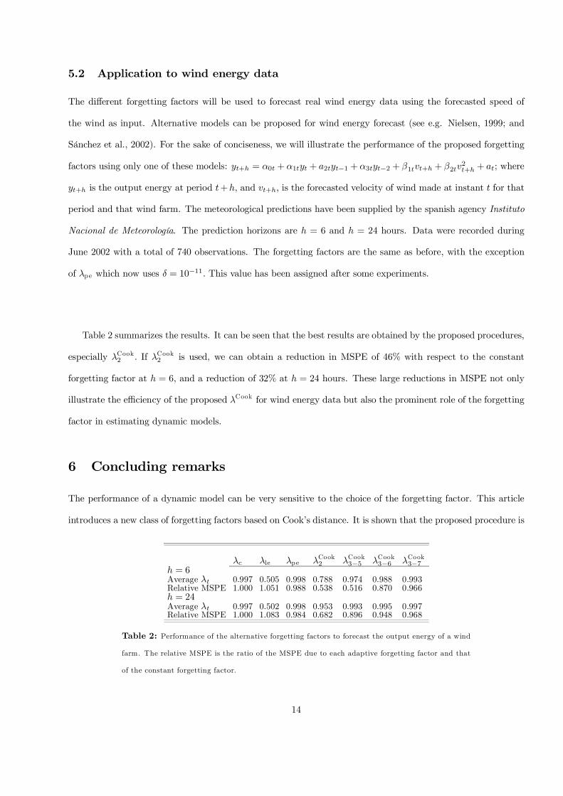
5.2 Application to wind energy data

The different forgetting factors will be used to forecast real wind energy data using the forecasted speed of

the wind as input. Alternative models can be proposed for wind energy forecast (see e.g. Nielsen, 1999; and

Sánchez et al., 2002). For the sake of conciseness, we will illustrate the performance of the proposed forgetting

factors using only one of these models: yt+h = α0t + α1tyt + a2tyt−1 + α3tyt−2 + β1tvt+h + β2tv2t+h + at; where

yt+h is the output energy at period t+h, and vt+h, is the forecasted velocity of wind made at instant t for that

period and that wind farm. The meteorological predictions have been supplied by the spanish agency Instituto

Nacional de Meteorología. The prediction horizons are h = 6 and h = 24 hours. Data were recorded during

June 2002 with a total of 740 observations. The forgetting factors are the same as before, with the exception

of λpe which now uses δ = 10−11. This value has been assigned after some experiments.

Table 2 summarizes the results. It can be seen that the best results are obtained by the proposed procedures,

especially λCook2 . If λCook2 is used, we can obtain a reduction in MSPE of 46% with respect to the constant

forgetting factor at h = 6, and a reduction of 32% at h = 24 hours. These large reductions in MSPE not only

illustrate the efficiency of the proposed λCook for wind energy data but also the prominent role of the forgetting

factor in estimating dynamic models.

6 Concluding remarks

The performance of a dynamic model can be very sensitive to the choice of the forgetting factor. This article

introduces a new class of forgetting factors based on Cook’s distance. It is shown that the proposed procedure is

λc λle λpe λCook2 λCook3−5 λCook3−6 λCook3−7h = 6Average λt 0.997 0.505 0.998 0.788 0.974 0.988 0.993Relative MSPE 1.000 1.051 0.988 0.538 0.516 0.870 0.966h = 24Average λt 0.997 0.502 0.998 0.953 0.993 0.995 0.997Relative MSPE 1.000 1.083 0.984 0.682 0.896 0.948 0.968

Table 2: Performance of the alternative forgetting factors to forecast the output energy of a wind

farm. The relative MSPE is the ratio of the MSPE due to each adaptive forgetting factor and that

of the constant forgetting factor.

14

able to adapt to situations where classical forgetting factors fail. Wind energy forecast is among those situations

where classical forgetting factors might fail. On the one hand, wind energy models can vary with the value

of the speed of the wind. In this setting, adaptive forgetting factors based on the leverage of the new input,

like λle , can be useful, whereas procedures based on the standardized prediction error, like λpe , might fail. On

the other hand, and due to meteorological variables, the parameters of a wind energy model can vary even

for a given value of wind speed. In this setting, adaptive forgetting factors based on the leverage of the new

input, like λle , are not adequate, but procedures based on the standardized prediction errors, like λpe , can be

satisfactory. It is seen in this article that Cook’s distance allows to build an adaptive forgetting factor that

embodies both approaches. Besides, the proposed forgetting factor is easy to use, and can be adapted to the

needs of a practitioner in a intuitive way.

15

References

[1] Cook, R.D. (1977), "Detection of Influential Observation in Linear Regression," Technometrics, 19, 15—18.

[2] Fortescue, T.R. Kershenbaum, L.S. and Ydstie, B.E. (1981), "Implementation of Self Tuning Regulators

with Variable Forgetting Factors," Automatica, 17, 831—835.

[3] Goodwin, G.C. and Sin, K.S. (1984), Adaptive Filtering Prediction and Control. Prentice Hall. New Jersey

[4] Grillenzoni, C. (1994), "Optimal Recursive Estimation of Dynamic Models," Journal of the American

Statistical Association, 89, 777—787.

[5] Grillenzoni, C. (2000), "Time-Varying Parameters Prediction," Annals of the Institute of Statistical Math-

ematics, 52, 108—122.

[6] Landau, I.D., Lozano, R., and M’Saad, M. (1998), Adaptive Control. Springer. Great Britain.

[7] Ljung. L. and Söderström, T. (1983), Theory and Practice of Recursive Identification. MIT Press, Cam-

bridge. Massachusetts.

[8] Nielsen, T.S. (1999), Using Meteorological Forecast in On-line Prediction of Wind Power. Institute of

Mathematical Modeling. Technical University of Denmark.

[9] Pollock, D.S.G. (1999), A Handbook of Time-Series Analysis, Signal Processing and Dynamics, Academic

Press. London.

[10] Sánchez, I., Usaola, J., Ravelo, O., Velasco, C., Dominguez, J., Lobo, M., González, G., Soto, F. (2002),

"Sipreólico: a Wind Power Prediction System Based on Flexible Combination of Dynamic Models. Appli-

cation to the Spanish Power System," Proceedings of the World Wind Energy Conference and Exhibition.

Berlin. Germany

16