ARXIV PREPRINT: THE ARTICLE IS PUBLISHED IN IEEE TRANS. INSTRUM. MEAS.VOL. 65, ISSUE: 3, MARCH 2016, DOI: 10.1109/TIM.2015.2508279 1 Recursive Discrete-time Models for Continuous Time Systems under Band-limited Assumptions Rishi Relan, Johan Schoukens, Fellow, IEEE , under contract 320378. Abstract—Discrete-time models are very convenient to simulate a nonlinear system on a computer. In order to build the discrete- time simulation models for the nonlinear feedback systems (which is a very important class of systems in many applications) described as y(t)= g1(u(t),y(t)), one has to solve at each time step a nonlinear algebraic loop for y(t). If a delay is present in the loop i.e y(t)= g2(u(t),y(t - 1)), fast recursive simulation models can be developed and the need to solve the nonlinear differential-algebraic (DAE) equations is removed. In this paper, we use the latter to model the nonlinear feedback system using recursive discrete-time models. Theoretical error bounds for such kind of approximated models are provided in the case of band-limited signals, furthermore a measurement methodology is proposed for quantifying and validating the output error bounds experimentally. Index Terms—Discrete-time models, nonlinear feedback sys- tems, Band-Limited signals and systems, One-Step ahead predic- tion, system identification. I. I NTRODUCTION:DISCRETE- TIME MODELING Modern measurement instruments make frequent use of advanced signal processing and control algorithms that are designed as well as implemented using discrete-time (non) linear models. Since most of the real-world systems evolve in continuous time, it should be carefully checked, if a discrete- time model can be used to describe such systems, and what errors might be created in the discretization step. Especially under the band-limited assumption (signals have no power above a given maximum frequency, for example measurements using anti-alias protection) this question becomes important. While for the linear systems, the error mechanism is well understood, it turns out that, it is not obvious how to quan- tify these errors for the nonlinear systems. This problem is addressed in this paper. This paper analyses first the nature of the error, and using these insights, it is shown how the measurement procedures can be designed in order to keep the error below an user specified level by making a proper choice for the sampling frequency. This is also an important and relevant problem for the instrumentation and measurement community since in many instruments nonlinear post- or pre-processing is done. Sensor linearization (e.g. for the relative humidity or temperature sen- sors) and nonlinear pre-compensation of actuators (Actuator nonlinearities can be static like friction, deadzone, saturation, The authors are with the ELEC Department, Vrije Universiteit Brus- sel (VUB),Brussels B-1050, Belgium (e-mail: [email protected], Jo- [email protected]). This work was supported in part by the Fund for Scientific Research (FWO-Vlaanderen), by the Flemish Government (Methusalem), the Belgian Government through the Inter university Poles of Attraction (IAP VII) Program, and by the ERC advanced grant Structured Nonlinear System Identification (SNLSID) and/or dynamic in nature like backlash and hysteresis due to the inaccuracy in the manufacturing of mechanical components and due to the nature of the physical laws [1]) [2], [3] are typ- ical examples. In modern instruments pre-compensation and linearization must be done on-board in real-time, hence use of a sophisticated numeric solver at each iteration is not feasible due to real-time constraints. Therefore discrete-time models for continuous-time systems with bounded output errors must be developed to deal with such constraints. Moreover, the goal of many measurement procedures is to build a discrete-time (nonlinear) simulation model for various real world systems such as gas sensing systems, gas turbine engines, large-signal amplifiers, RF thermistors etc. [4]–[9]. Discrete-time models for linear and non-linear dynamical systems can be developed under different assumptions of the measurement set-up, e.g. the zero-order hold (ZOH) and the band-limited measurement set-up. A. Linear Systems 1) Zero-order hold measurement set-up: In the case of a zero-order hold (ZOH) measurement set-up, as shown in Fig.1, the linear-time invariant system [10] can be described using the discrete-time representation: y(t)= ∞ X k=1 g(k)u(t - k) (1) Fig. 1: Zero-order hold (ZOH) measurement set-up 2) Band-limited measurement set-up: For the band-limited measurement setup, as shown in Fig.2, the discrete-time rep- resentation of the system can be written as y(t)= ∞ X k=0 g(k)u(t - k) = g(0)u(t)+ ∞ X k=1 g(k)u(t - k) (2) arXiv:1805.05040v1 [cs.SY] 14 May 2018

Welcome message from author
This document is posted to help you gain knowledge. Please leave a comment to let me know what you think about it! Share it to your friends and learn new things together.
Transcript
ARXIV PREPRINT: THE ARTICLE IS PUBLISHED IN IEEE TRANS. INSTRUM. MEAS.VOL. 65, ISSUE: 3, MARCH 2016, DOI: 10.1109/TIM.2015.2508279 1
Recursive Discrete-time Models for ContinuousTime Systems under Band-limited Assumptions
Rishi Relan, Johan Schoukens, Fellow, IEEE , under contract 320378.
Abstract—Discrete-time models are very convenient to simulatea nonlinear system on a computer. In order to build the discrete-time simulation models for the nonlinear feedback systems (whichis a very important class of systems in many applications)described as y(t) = g1(u(t), y(t)), one has to solve at each timestep a nonlinear algebraic loop for y(t). If a delay is present inthe loop i.e y(t) = g2(u(t), y(t − 1)), fast recursive simulationmodels can be developed and the need to solve the nonlineardifferential-algebraic (DAE) equations is removed. In this paper,we use the latter to model the nonlinear feedback system usingrecursive discrete-time models. Theoretical error bounds forsuch kind of approximated models are provided in the case ofband-limited signals, furthermore a measurement methodology isproposed for quantifying and validating the output error boundsexperimentally.
Index Terms—Discrete-time models, nonlinear feedback sys-tems, Band-Limited signals and systems, One-Step ahead predic-tion, system identification.
I. INTRODUCTION: DISCRETE-TIME MODELING
Modern measurement instruments make frequent use ofadvanced signal processing and control algorithms that aredesigned as well as implemented using discrete-time (non)linear models. Since most of the real-world systems evolve incontinuous time, it should be carefully checked, if a discrete-time model can be used to describe such systems, and whaterrors might be created in the discretization step. Especiallyunder the band-limited assumption (signals have no powerabove a given maximum frequency, for example measurementsusing anti-alias protection) this question becomes important.While for the linear systems, the error mechanism is wellunderstood, it turns out that, it is not obvious how to quan-tify these errors for the nonlinear systems. This problem isaddressed in this paper. This paper analyses first the natureof the error, and using these insights, it is shown how themeasurement procedures can be designed in order to keep theerror below an user specified level by making a proper choicefor the sampling frequency.
This is also an important and relevant problem for theinstrumentation and measurement community since in manyinstruments nonlinear post- or pre-processing is done. Sensorlinearization (e.g. for the relative humidity or temperature sen-sors) and nonlinear pre-compensation of actuators (Actuatornonlinearities can be static like friction, deadzone, saturation,
The authors are with the ELEC Department, Vrije Universiteit Brus-sel (VUB),Brussels B-1050, Belgium (e-mail: [email protected], [email protected]). This work was supported in part by the Fundfor Scientific Research (FWO-Vlaanderen), by the Flemish Government(Methusalem), the Belgian Government through the Inter university Polesof Attraction (IAP VII) Program, and by the ERC advanced grant StructuredNonlinear System Identification (SNLSID)
and/or dynamic in nature like backlash and hysteresis due tothe inaccuracy in the manufacturing of mechanical componentsand due to the nature of the physical laws [1]) [2], [3] are typ-ical examples. In modern instruments pre-compensation andlinearization must be done on-board in real-time, hence use ofa sophisticated numeric solver at each iteration is not feasibledue to real-time constraints. Therefore discrete-time modelsfor continuous-time systems with bounded output errors mustbe developed to deal with such constraints. Moreover, the goalof many measurement procedures is to build a discrete-time(nonlinear) simulation model for various real world systemssuch as gas sensing systems, gas turbine engines, large-signalamplifiers, RF thermistors etc. [4]–[9]. Discrete-time modelsfor linear and non-linear dynamical systems can be developedunder different assumptions of the measurement set-up, e.g.the zero-order hold (ZOH) and the band-limited measurementset-up.
A. Linear Systems
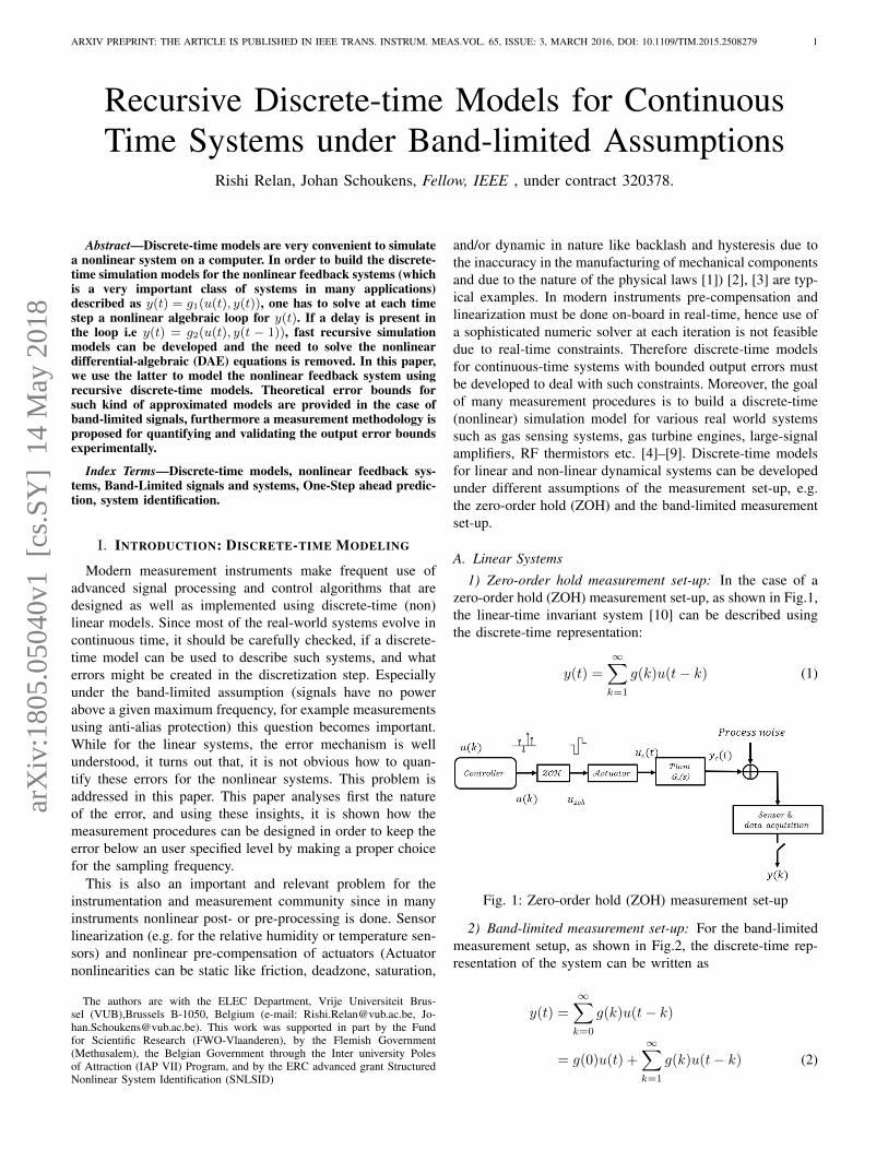
1) Zero-order hold measurement set-up: In the case of azero-order hold (ZOH) measurement set-up, as shown in Fig.1,the linear-time invariant system [10] can be described usingthe discrete-time representation:
y(t) =
∞∑k=1
g(k)u(t− k) (1)
Fig. 1: Zero-order hold (ZOH) measurement set-up
2) Band-limited measurement set-up: For the band-limitedmeasurement setup, as shown in Fig.2, the discrete-time rep-resentation of the system can be written as
y(t) =
∞∑k=0
g(k)u(t− k)
= g(0)u(t) +
∞∑k=1
g(k)u(t− k) (2)
arX
iv:1
805.
0504
0v1
[cs
.SY
] 1
4 M
ay 2
018

ARXIV PREPRINT: THE ARTICLE IS PUBLISHED IN IEEE TRANS. INSTRUM. MEAS.VOL. 65, ISSUE: 3, MARCH 2016, DOI: 10.1109/TIM.2015.2508279 2
Fig. 2: Band-limited measurement set-up
It can be seen in (1) that it does not contain any directterm i.e g(0) term. This kind of representation is very popularin discrete-time control systems whereas the discrete-timerepresentation (2) contains the direct-term. This kind of modelrepresentation is very popular in the digital signal processingcommunity and it is more appropriate for simulation as wellas measurement applications.
B. Nonlinear Systems
One would reasonably expect similar results to hold for thenonlinear systems. However, the situation for the nonlinearcase is more complex than for the linear systems. In the caseof a zero-order hold (ZOH) measurement set-up, we wouldlike to write the output of the system as
y(t) = g1(ut−1, yt−1) (3)
where ut = [u(t), u(t − 1), ......u(1)] and yt = [y(t), y(t −1), ......y(1)]. In general this does not hold true for e.g.nonlinear feedback systems. In the case of nonlinear feedbacksystems (3) becomes y(t) = g1(ut, yt) and one needs tosolve nonlinear algebraic loops due to the presence of adirect-term. Also for the band-limited measurement set-upsimilar constraints exist. The questions which we would liketo raise is whether we can approximate y(t) = g1(ut, yt)by y(t) = g1(ut−1, yt−1), and how the approximation errordepends on the experimental conditions.
Consider for example a nonlinear feedback system as shownin Fig.3, where Gc(s) is a Laplace transfer function betweenthe input signal xc(t) and the output signal yc(t). φ(∗) is anymemory-less, static non-linearity in the feedback loop. Manyelectrical, electronic and physical systems, e.g. oscillators [11],biomedical [12] and mechanical system [13]–[15], contain inan implicit manner, a nonlinear feedback loop and can bedescribed using the similar model structure.
Fig.4 shows a possible model structure for a discrete-timerepresentation of the continuous-time system in Fig.3. Fora band-limited input signal uc(t) (see later for a precisedefinition), the linear system G(s) can be approximated bya discrete-time model
y(t) =
∞∑k=0
g(k)x(t− k), (4)
Fig. 3: Nonlinear feedback system: continuous time
Fig. 4: Nonlinear feedback system: discrete-time
and q−1(one sample delay operator) provided that the sam-pling frequency fs is sufficiently high such that the aliasingerrors are acceptably small. For a given sampling periodTs = 1
fs, the discrete-time signals u and y can be represented
as
u(k) = uc(kTs) ; y(k) = yc(kTs). (5)
The output of the discrete-time model described by Fig.4can be written as
y(t) = g(q, θ)(u(t)− φ(y(t))). (6)
This is an example of a nonlinear algebraic loop [16], whichimplies that a set of nonlinear differential-algebraic equations(DAE) should be solved at each time step in order to calculatethe model output. In the control engineering community,many approaches dealing with discrete-time representationof continuous-time systems implicitly assume that the directterm is equal to zero, in order to deal with the problem. Inprinciple, this problem (of continuous time system modellingand simulation) can be tackled by utilising dedicated numeric(integration) solvers. The main disadvantage of using a numer-ical integration solver is, that it can have multiple solutions.In fact, it is even possible that no solution exists [17].Moreover, it is a very time consuming approach as well as therobustness of the obtained solution can not be guaranteed [18],[19] therefore these models are not well suited for real-timeapplications. Interested readers are referred to the Section IIfor a brief introduction to the literature dealing with the issuesof sampled data models within the control system community.The identification of block-oriented nonlinear feedback modelsreceived considerably less attention and still is in its infancy.To the best of authors knowledge, this issue of (how to avoid)
ARXIV PREPRINT: THE ARTICLE IS PUBLISHED IN IEEE TRANS. INSTRUM. MEAS.VOL. 65, ISSUE: 3, MARCH 2016, DOI: 10.1109/TIM.2015.2508279 3
nonlinear algebraic loop has not been tackled before in theinstrumentation and measurement community.
The authors in [20]–[22] used block-oriented nonlinearfeedback structure to model a microwave crystal detectorRF applications, but it turns out that the nonlinear algebraicloop created convergence problems for larger inputs. In orderto avoid the nonlinear algebraic loops while developing thediscrete-time nonlinear linear fractional representation (LFR)model (representation of nonlinear feedback systems), theauthors in [23]–[27] assumed that the one tab delay is presentimplicitly in the loop or in other words the direct feed-throughterm is 0. The authors did not check the validity (neithertheoretically nor experimentally) of their assumption. Thisassumption fails under the band-limited measurement condi-tions as explained above, whereas [28] proposed a solutionby means of geometrical transformation of the nonlinearitiesand algebraic transformation of the time-dependent equationsin order to deal with algebraic loops in nonlinear acousticsystems. This approach may not be optimal for fast recursivemodels intended for real-time scenarios.
Hence, the main idea in this paper is to show under whichexperimental conditions and constraints we can develop adiscrete-time recursive simulation model. To do this in asimple (similar) way, we can impose one sample delay forthe linear block or, equivalently g(0) in (4) will be set tozero. Taking into account the imposed delay, we will obtainthe following model equation
y(t) =
∞∑k=1
g(k)x(t− k)
x(t) = u(t)− y(t)
y(t) =
∞∑k=1
g(k)(u(t− k)− φ(y(t− k)) (7)
Under the band-limited assumption this discrete-time represen-tation is a recursive in nature. Hence, we can develop the re-cursive discrete-time simulation models by forcing the direct-term of the identified model equal to 0, i.e. by introducingexplicitly a delay in to the loop. In order to do this, someassociated questions need to be answered:• How to quantify the errors associated with the approxi-
mated models ?• What are the different factors/parameters which can in-
fluence the errors ?• How can we keep the error in the approximated model
small enough by choosing the appropriate experimentalconditions ?
In order to answer these questions, in this paper, we proposea measurement approach to analyse and bound the outputerror of the developed discrete-time model for band-limitedmeasurements. The rest of the paper is organized as fol-lows. Section II gives an overview about the identification ofthe sampled-data models. Section III formalizes the problemstatement and provides a comprehensive theoretical analysisof the errors associated with approximated linear discrete-time models with direct-term equal to 0. Section IV gives
an overview of an experimental investigation performed inorder to validate the obtained theoretical bounds on the errorqualitatively both for linear as well as nonlinear (nonlinearfeedback) dynamical systems and Conclusions are formulatedin Section V.
II. SAMPLED DATA MODELS: GENERAL REMARKS
Identification of continuous-time systems from sampleddata [29] is a problem of considerable importance in thecontrol system community. These discrete-time representationsof the continuous time system can be developed under a zero-order hold (ZOH) or band-limited (BL) assumption of theinter-sample behaviour [30]. Exact discrete-time models ofa continuous time systems at the sampling instances can beobtained for the linear systems by assuming a zero-order hold(ZOH) input [31]–[33]. This argument may, however, lead toa false sense of security when using sampled data as the pole-zeros patterns of the discrete-time systems may not be similardue to the presence of the extra zeros called, sampling zeros,in the associated discrete-time transfer function, which is theconsequence of the sampling process. These zeros have nocounterpart in the underlying deterministic continuous-timemodel [34]. Further in-depth information about the sampleddata models for linear (Non-linear) deterministic (Stochastic)system with different sample and hold characterizations canbe found in [35]–[42] and the references mentioned therein.For the purpose of this study, this is not so important, ashere we focus on the input-output behaviour of the underlyingsystem at the discrete-time samples. Most of the previous workassumes that the data is gathered under the zero-order holdassumption.
In these ZOH models, no direct term is present for thelinear system, see also (1). As explained earlier, most ofthese assumptions do not hold true for complex nonlineardynamical systems, including networked dynamical systems,as the signals in the loop are no longer ZOH. Hence, itis important to consider discrete-time models under band-limited measurement assumptions. Even under band-limitedassumptions, an arbitrary good discrete-time representationof the underlying continuous-time system can be retrieved.However, in that case, the direct term will be different fromzero. The main emphasis of this study is to analyze the impactof explicitly setting this term to zero. The resulting error willnot only depend on the signal properties (Band-limited inthis study), but also on the relative degree of the underlyingcontinuous-time system. Indeed as the sampling rate increases,a continuous-time system with relative degree d ≥ 2 behavesas an dth order integrator 1
sdbeyond Nyquist frequency.
Therefore, the impulse response will depart very slowly fromzero. The direct term in the discrete-time representation ofsuch continuous-time models will be small, and will diminishto zero as the sampling frequency is increased. In the nextsection, under the band-limited measurement assumptions, adetailed analysis of the error associated with the discrete-timemodels with direct term equal to 0 is provided.
ARXIV PREPRINT: THE ARTICLE IS PUBLISHED IN IEEE TRANS. INSTRUM. MEAS.VOL. 65, ISSUE: 3, MARCH 2016, DOI: 10.1109/TIM.2015.2508279 4
III. THEORETICAL ANALYSIS
A. Proposed Methodology
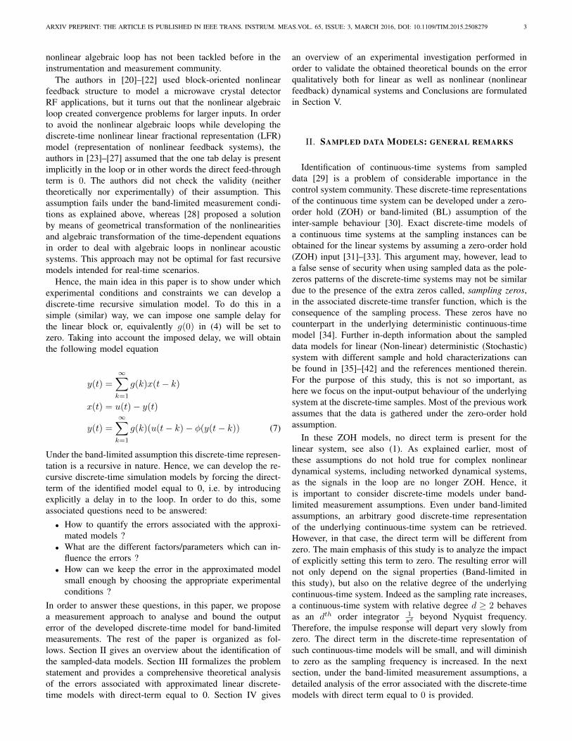
In this section, we provide a thorough theoretical analysisbased on the preliminary experimental investigations per-formed by [43] using the measurement methodology as shownin Fig.5. In this section under the band-limited measurementset-up assumptions, error bounds for the approximated lineardiscrete-time models with the direct-term set equal to 0 willbe provided.
Fig. 5: Proposed methodology for the error quantification
The aim in this study is to identify the discrete-time modelGd(k), with direct-term gd(0) forced equal to 0, from thesampled measurements u(kTs), y(kTs) of the continuous-time plant Gc(s), with input signal uc and output signalyc, under band-limited measurement conditions. Ts is thesampling period. uc can be an output from an actuator ora generator filter Fc(s) which in turns can be excited by anarbitrary signal, e.g. white noise, random-phase multisines orany zero-order hold (ZOH).
The main aspects which can influence the magnitude of theerror in the output signal of the identified discrete-time modelare:• Is it possible to make an accurate prediction about the
future input uc given its past sampled values i.e. u(t|t−1)?
• How much is the error e(t) that would be introducedin case we can not make a perfect or accurate enoughprediction of the input u(t) = u(t) + e(t) ?
• What is the influence of the error in the one-step aheadprediction u(t|t − 1) and of the direct g(0)u(t) term onthe final output signal of the discrete-time model i.e. y(t)in (2) ?
The reasoning mentioned above holds equally true in the caseof block-oriented nonlinear feedback models as discussed inI-B, because there are band-limited signals in the loop, henceit is enough for one system to have a delay to break thenonlinear algebraic loop. Hence, the first step in the analysisis to quantify the error in the one-step ahead prediction ofthe input signal u(t) for a band-limited input signal. Next weanalyse the effect on the system’s output.
B. Error Analysis
In this section, first a brief introduction to the band-limitedsignals and processes is given. Thereafter, to address the
problem, the following steps mentioned below will be taken.
1) quantification of the one-step ahead prediction error inthe case of a perfectly BL signal u(t);
2) quantification of the one-step ahead prediction error inthe case of an actual BL signal u(t), e.g., filtered ZOHsignal;
3) quantification of the error in the final output signal y(t).
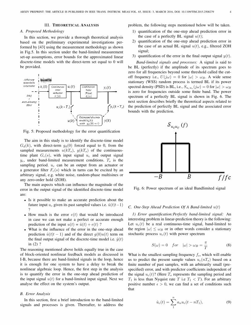
Band-limited signals and processes: A signal is said tobe BL (perfectly) if the amplitude of its spectrum goes tozero for all frequencies beyond some threshold called the cut-off frequency i.e., U(jω) = 0 for |ω| > ωB . A wide sensestationary (WSS) random process is termed BL if its powerspectral density (PSD) is BL, i.e., Sucuc(jω) = 0 for |ω| > ωBis zero for frequencies outside some finite band. The powerspectrum of a perfectly BL signal is shown in Fig. 6. Thenext section describes briefly the theoretical aspects related tothe prediction of perfectly BL signal and the associated errorbounds with the prediction.
Fig. 6: Power spectrum of an ideal Bandlimited signal
C. One-Step Ahead Prediction Of A Band-limited u(t)
1) Error quantification:Perfectly band-limited signal: Aninteresting problem in linear-prediction theory is the following:Let uc(t) be a real continuous-time signal, band-limited tothe region |ω| ≤ ωB or in other words consider a stationarystochastic process uc(t) with power spectrum
S(ω) = 0 for |ω| > ωB =π
T(8)
What is the smallest sampling frequency fs, which will enableus to predict the present sample values uc(nTs) based on afinite number of past samples, with an arbitrarily small (pre-specified) error, and with predictor coefficients independent ofthe signal uc(t)? (Here Ts represents the sampling period andT1 is less than Nyquist rate T i.e T1 < T ). For an arbitrarypositive number ε > 0, we can find a set of conditions suchthat
uc(t) =
n∑1
anuc(t− nT1), (9)

ARXIV PREPRINT: THE ARTICLE IS PUBLISHED IN IEEE TRANS. INSTRUM. MEAS.VOL. 65, ISSUE: 3, MARCH 2016, DOI: 10.1109/TIM.2015.2508279 5
E
∥∥∥∥∥(uc(t)−
n∑1
anuc(t− nT1)
)∥∥∥∥∥2 < ε1. (10)
For band-limited processes with absolutely continuous spectralmeasure i.e., processes with spectral density, Wainstein andZubakov [44] proved that if the sampling rate is increasedat least three times above the Nyquist rate a band-limitedprocess can be predicted with arbitrarily small error from itspast samples using an universal formula for the predictor. Abetter result in this direction is [45], where a similar predictoris constructed when the samples are taken at twice the Nyquistrate. This sequence of predictors converges with exponentialrate. However, it could be more difficult to find explicit coef-ficients for the predictor. These results were further improvedby Splettstosser [46] in 1982, who showed that this kind ofprediction is possible even with the sampling frequency equalto 1.5 times the Nyquist frequency.
Brown [45] and Splettstosser [46] have also observed thatit is theoretically possible to predict the samples of uc(t) inthe above manner, as long as the sampling frequency is largerthan the Nyquist rate by any arbitrarily small amount ε2 > 0.This observation has also been made by Papoulis [47] who hasgiven a different proof showing that the greatest lower boundof the prediction error is zero.
G.L.B.Ean
E
∥∥∥∥∥(uc(t)−
∞∑1
anuc(t− nT1)
)∥∥∥∥∥2 = 0.
(11)Further references, and proofs can be found in [48], [49], andthe references contained therein. The result presented in [49]and [47] are in fact particular cases of [50]. This discussionconcludes that a band-limited signal can be perfectly predictedfrom its past values (samples) provided that the samplingfrequency fs is larger that the Nyquist rate by any arbitrarilysmall amount ε > 0.
2) Error quantification:Low-pass filtered signal: But inpractice it is impossible to have a perfectly band-limited signal.In practice, a band-limited signal uc(t) can be considered tobe made of two parts: ubl(t) a part of the signal which canbe perfectly predicted, and uε(t) which can not be predictedor remains unexplained as shown in Fig.7
uc(t) = ubl(t) + uε(t)
Therefore the lower bound of the one-step ahead predictionerror would be:
E[e(t)2
]≤ E
[uε(t)
2]
(12)
Further in the discussion below a concise theoretical expla-nation is given to quantify as well as to identify the factorsassociated with the error in a one-step ahead prediction of anactual band-limited signal.
Fig. 7: Power spectrum of an actual bandlimited signal
3) One-step ahead prediction of an actual band-limitedu(t): Consider the case of a low pass filter Fc(s) shown inFig.8. for example, a Butterworth or a Chebyshev filter oforder n, with cut-off frequency fc, excited by white noiseinput signal.
Fig. 8: Analysis of one-step ahead prediction
From the literature it is a well known fact that gain of thelow-pass filter in the roll-off region varies as a factor of
(f
fc
)−n≈∣∣∣∣Fc( ffc
)∣∣∣∣ ,where f is the frequency of the signal, fc is the cut-offfrequency, and n the filter order [see Fig.9]. The filter roll-offbeyond the cut-off frequency is usually defined in dB/decade.
Fig. 9: Error in an actual signal
a) Filtered White Noise: The Power (Puεuε) containedin the unexplained part of a band-limited signal generated byfiltering white noise signal can be calculated by integratingthe signal over the frequency band [fs − fc,∞[ i.e.

ARXIV PREPRINT: THE ARTICLE IS PUBLISHED IN IEEE TRANS. INSTRUM. MEAS.VOL. 65, ISSUE: 3, MARCH 2016, DOI: 10.1109/TIM.2015.2508279 6
Puεuε ∼= 2
∫ ∞fs−fc
(fcf
)2n
df
∼=2fc
2n− 1
(fc
fs − fc
)2n−1
∼=2fc
2n− 1
(fcfs
)2n−1
(13)
because fs − fc ∼= fs as fs fc. From (13) it can beconcluded that the power in the unexplained part of the band-limited signal uc(t) varies as
Puεuε = O(fcfs
)2n−1
(14)
b) ZOH White Noise: In the case of the zero-order-hold (ZOH), the excitation signal is considered to be constantbetween consecutive samples. As seen from the envelope inthe Fig.10 [30] , the envelope of Sucuc for f
fs> 1 is ( ffs )−2,
hence the zero-order hold (ZOH) will create an additional roll-off and therefore it will not increase the order of magnitudeof the error given in (14) .
Fig. 10: ZOH Spectrum
c) Conclusion: Therefore from the analysis above it canbe concluded that
Puεuε =
[∣∣∣u(t)− ˆu(t)∣∣∣2] ≤ O(fc
fs
)2n−1
(15)
for an all pole generator filter/actuator, independent of theZOH or BL measurement of the signal.
4) Error quantification of the output of a linear system:The next step in the analysis of error is to observe the impactof the error in the one-step ahead prediction of u(t) on thefinal output y(t) of the discrete-time model. The next sectionprovides a concise theoretical explanation of the impact ofthe error in u(t) on the final output y(t). For the purpose ofquantifying the impact of the error in u(t) on the final outputy(t) the following assumptions are made:
Assumption 1: The data can be acquired at sufficiently highsampling rates and effect of sampling zeros, folding, etc. canbe neglected.
Remark: This can also be resolved using virtually upsam-pling the data.
Assumption 2: The discrete-time model representation ofthe continuous-time system with any arbitrary relative degreeequal to d will be close to the impulse invariant transform(I.I.T) [51]–[55] of the continuous-time impulse response asshown in Fig.11 and Fig.12 respectively.
Remark: The theoretical analysis is based on the discrete-time impulse response representation of the continuous timesystem, but it is equally valid for any other discrete-time modelrepresentation.
Fig. 11: Impulse response for system with rel. degree = 1
Fig. 12: Impulse response for system with rel. degree > 1
D. Impact Of The Error In u(t) On The Final Output y(t)
Using the initial-value theorem of the Laplace transform,the impulse response gc(t) of the continuous time system withrelative degree d > 1 [56]–[58] meets.
gcd−1(t)
∣∣∣t=0
= 0 (16)
The output of the identified discrete-time model can be ex-pressed as:
y(t) =
∞∑k=0
gd(k)ud(t− k)
∼=∞∑k=0
gc(kTs)ud(t− k) (17)
Where gd(k) = gc(kTs) due to impulse invariant transforma-tion. From (16) it follows that gd(0) will converge to zero ifd ≥ 2, for fs →∞. In the rest of this paper, we assume that|gd(0)| < M , where M is a bounded value of the responseand if d ≥ 2 then lim
fs→∞M = 0, .

ARXIV PREPRINT: THE ARTICLE IS PUBLISHED IN IEEE TRANS. INSTRUM. MEAS.VOL. 65, ISSUE: 3, MARCH 2016, DOI: 10.1109/TIM.2015.2508279 7
The output y(t) can further be expanded as described by(18), where u(t) is the one-step ahead prediction of the inputsignal u(t).
y(t) =1
fsgd(0)u(t) +
1
fs
∞∑k=1
gd(kTs)u(t− k) (18)
From (17) and (18), the error in the output signal can bewritten as
yε(t) = y(t)− y(t)
=1
fsg(0)uε (19)
Furthermore the power contained in the output error signal canbe expressed as
Pyε =
(1
fs
)2
g(0)2Puε
=
(1
fs
)2
g(0)2O(fcfs
)2n−1
(20)
This implies that the root mean squared error in yεRMS isupper-bounded by
yεRMS ≤1
fsO(fcfs
)n− 12
(21)
(20) and (21) above describe a relationship between the cut-off frequency of the generator filter, the sampling frequencyand the error in the output as well as the unmodelled part ofthe input signal respectively. In the next section a qualitativeexperimental investigation has been performed to validate thistheoretical analysis.
IV. EXPERIMENTAL VERIFICATION
In order to validate the theoretical results qualitatively,real-world experimental investigations were performed. In thesections below, first the measurement set-up is introduced,next the experiment design is explained, and finally the resultsare discussed. A preliminary findings of the results has beenalready presented in the [43]
A. Measurement Set-up
Fig. 13: Experimental set-up
1) Linear System: Fig.13 demonstrates the schematic ofthe experimental set-up and the measurement architecture forthis validation study. For the sake of simplicity a R−C filteris selected as the continuous-time plant to be identified inthe experiment involving the identification of a linear system.Since in this case the relative degree d = 1, it is a worst caseexample because g(0) will be the dominant term in the impulseresponse. In general, it can be any other real continuous-time system. xc(t) denotes the ideal reference signal fromthe function generator whereas uc(t) and yc(t) are the actualcontinuous time input and the output signal of the plantrespectively .
2) Nonlinear system: In the case of a nonlinear system,the plant shown in Fig.13 is replaced by the Silverbox whilekeeping the other experimental set-up/measurement methodol-ogy the same. The Silverbox is an electrical circuit, simulatinga mass-spring-damper system. It is an example of nonlineardynamic system with feedback as shown in Fig.14, wherethe linear contributions are dominant for the small excitationlevels of the input signal [59]. The system’s behaviour can beapproximately described by the following equation:
Fig. 14: Silverbox Dynamics
my(t) + dy(t) + k1y(t) + k3y3(t) = u(t) (22)
where u(t) represents the input force applied to the mass m,and the output y(t) is the mass displacement. Parameters k1and k3 describe the (nonlinear) behavior of the spring, and dis the damping of the system [30].
As shown in the measurement set-up in Fig.13, the signalsare generated by an arbitrary waveform generator (AWG) orfunction generator, the Agilent/HP E1445A, with an internalreconstruction filter that has a cut-off frequency at 250 kHz.The output of the generator filter is filtered by a 4th − orderWavetek Dual Hi/low pass (Model 432) filter with a cut-offfrequency of 100 Hz. The input and output signals of theplant (analog RC Filter with a cut-off frequency of 1kHz/ Silverbox) are measured by the alias protected acquisitionchannels (Agilent/HP E1430A). The AWG and acquisitioncards are clocked by the AWG clock, and hence the acquisitionis phase coherent to the AWG. Finally, buffers are addedbetween the acquisition cards and the input and output ofthe device under test (DUT) to impose impedance isolationof the signals. The buffers are added to match the 50 Ωinput impedance of the Agilent/HP E1430A VXI modulesacquisition channels to a high impedance input. The buffersare very linear ( ≈ 85 dBc at full scale and 1 MHz) up to 10V peak to peak, and have an input impedance of 1 MΩ and a50 Ω output impedance.
ARXIV PREPRINT: THE ARTICLE IS PUBLISHED IN IEEE TRANS. INSTRUM. MEAS.VOL. 65, ISSUE: 3, MARCH 2016, DOI: 10.1109/TIM.2015.2508279 8
B. Experiment Design
A normally distributed noise signal (white noise) is used asan input excitation signal for the identification of the linearmodel, and for the identification of the polynomial nonlinearstate-space (PNLSS) model. An odd-random phase multisinesignal [30] is used to excite the Silverbox in the frequencyband of [0-100 Hz]. In an odd-random phase multisine signal,only the odd frequency lines are excited with the user-definedamplitude levels. The even frequency lines as well as thenon-excited odd lines, then act as the detection lines for thedetection of system nonlinearities. The choice of the inputexcitation signal is not only restricted to these two classesof signals, rather one can also use any persistently excitingsignal such as e.g. a flat spectrum random phase multisineor a uniformly distributed noise signal as an input excitationsignal. We make this choice in order to verify the level ofthe nonlinear distortions during the experiment. The excitationsignal has a period of 78125 samples. The level of the inputexcitation is zero mean with a standard deviation 0.99 V for thefirst experiment involving the identification of the linear modeland the amplitude of the full odd random phase multisine iszero mean with a standard deviation of 127mV during theidentification of the polynomial nonlinear state-space (PNLSS)model. The three different experiments performed in thisinvestigation are:
1) The one-step ahead prediction of the genera-tor/actuator signal u(t): For the one-step ahead predic-tion the data is acquired for P = 1 period at differentbandwidths of the generator filter/actuator while keepingthe sampling frequency fs constant at 78.125 kHz. Forthe sake of brevity an Auto-regressive with an exogenousinput (ARX) model structure is chosen for the one-step ahead prediction. The one-step ahead prediction isperformed at different bandwidths of the generator filteras well as for different model orders.
2) Identification of a discrete-time model based on thesampled uc(t) and yc(t): P = 2 periods of data isacquired at a sampling frequency fs of 156.25 kHzfor the model identification experiment at a constantgenerator filter/actuator bandwidth. The data is down-sampled virtually for identifying discrete-time models atthe different sampling frequencies. For the identificationof the discrete-time model, the Output-error (OE) modelstructure (y(t) = B(q)
F (q)u(t − nk) + e(t)) is chosen forthe same reasons. During the identification of the modelwith B0 = 0, the complexity (order) of the model wasslightly increased (numerator nb = 2, denominator nf =4 from numerator nb = 2, denominator nf = 2 with B0
term intact) to accommodate the extra dynamics.3) Identification of a polynomial nonlinear state-space
(PNLSS) discrete-time model based on the sampleduc(t) and yc(t):. In order to identify the discrete-time nonlinear model for the silverbox, the polynomialnonlinear state-space model structure [60] is selectedbecause it implicitly embeds the delay in its modelstructure as described below:
x(t+ 1) = Ax(t) +Bu(t) + Eζ(t) (23)
y(t) = Cx(t) +Du(t) + Fη(t) (24)
The coefficients of the linear terms in x(t) and u(t) aregiven by the matrices A ∈ Rna×na and B ∈ Rna×nuin the state equation, C ∈ Rny×na and D ∈ Rnu×nain the output equation. The vectors ζ(t) ∈ Rnζ andη(t) ∈ Rnη contain nonlinear monomials in x(t) andu(t) of degree two up to a chosen degree P . Thecoefficients associated with these nonlinear terms aregiven by the matrices E ∈ Rna×nζ and D ∈ Rny×nη .Note that the monomials of degree one are included inthe linear part of the PNLSS model structure. P = 2periods of data for M = 10 different realisations of theodd random phase multisine input excitation is acquiredat a sampling frequency fs of 78.125 kHz for themodel identification experiment at a constant generatorfilter/actuator bandwidth. M = 9 realisations are usedfor the training purpose whereas M = 1 realisation iskept aside to test the model performance on an unseenvalidation data. For the analysis purpose, the sampleddata was virtually down-sampled at different samplingrates by explicitly omitting the samples.
C. Results
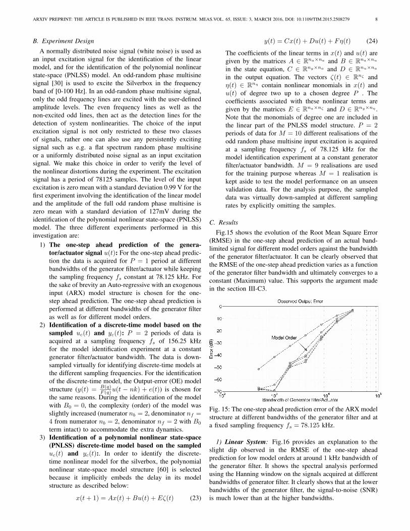
Fig.15 shows the evolution of the Root Mean Square Error(RMSE) in the one-step ahead prediction of an actual band-limited signal for different model orders against the bandwidthof the generator filter/actuator. It can be clearly observed thatthe RMSE of the one-step ahead prediction varies as a functionof the generator filter bandwidth and ultimately converges to aconstant (Maximum) value. This supports the argument madein the section III-C3.
Fig. 15: The one-step ahead prediction error of the ARX modelstructure at different bandwidths of the generator filter and ata fixed sampling frequency fs = 78.125 kHz.
1) Linear System: Fig.16 provides an explanation to theslight dip observed in the RMSE of the one-step aheadprediction for low model orders at around 1 kHz bandwidth ofthe generator filter. It shows the spectral analysis performedusing the Hanning window on the signals acquired at differentbandwidths of generator filter. It clearly shows that at the lowerbandwidths of the generator filter, the signal-to-noise (SNR)is much lower than at the higher bandwidths.

ARXIV PREPRINT: THE ARTICLE IS PUBLISHED IN IEEE TRANS. INSTRUM. MEAS.VOL. 65, ISSUE: 3, MARCH 2016, DOI: 10.1109/TIM.2015.2508279 9
Fig. 16: The power spectrum of the measured uc at thedifferent bandwidths of the generator filter for a fixed samplingfrequency fs = 78.125 kHz. It is evident from the figurethat the signal around the cut-off frequency (1kHz) of RCfilter is not persistently exciting (due to poor SNR) for theidentification of the linear model
The Fig.17, shows the frequency spectrum of the input andoutput signals of the linear system and the results obtainedfrom the identification of the discrete-time model for thecontinuous time first order linear dynamical system with andwithout forcing the direct term gd(0) = 0 are shown in Fig.18.It is clearly observed that the influence of explicitly forcingthe direct-term gd(0) = 0 diminishes very quickly, if thedata is acquired at sufficiently high sampling frequencies. It isclearly seen that the slope of the error curve with B0 = 0 isapproximately ≈ −75dB/decade. The theoretical predictionmade in Section III-D, corresponds to ≈ −90dB/decadebecause the 1st − order linear system was excited by thewhite Gaussian noise filtered with a 4th − order low-passfilter. The observed drop in error is slightly less than as perthe theoretical prediction. The reason behind this can easily beunderstood by carefully looking at the Fig.17, which clearlyshows that the input excitation rolls-off very slowly above10kHz. This is a voilation of the low-pass assumption that ismade in the developed theroy, hence along with the presenceof the measurement noise, it hinders the achievement of theerror bound predicted by the theory exactly.
Fig. 17: Spectrum of the input and output signals of the linearsystem
The RMSE of the discrete-time model with forced delayterm reduces very quickly afterwards with respect to thesampling frequency and ultimately converges to the same min-imum value (lower bound) which is observed while keepingthe direct term intact during the identification of discrete-timemodel of a particular pre-specified model order as well asmodel structure.
Fig. 18: Output error of the linear model
2) Non-linear System: The results obtained from the iden-tification of the polynomial nonlinear state-space (PNLSS)model is shown in Fig.20. As discussed earlier, this particulardiscrete-time model structure implicitly embeds the forceddelay term.
Fig. 19: The input and output spectrum of the nonlinearsilverbox system
Fig.19 shows the input and output spectrum of the silverboxdynamics excited by an odd random phase multisine inputsignal. From the output spectrum, it can be observed that thefirst resonance peak of the system lies at around ≈ 70Hz. Inorder to completely capture the information about this reso-nance peak inside the PNLSS discrete-time model structure,we must at least sample the input and output signals at atleast≈ 140Hz or at a greater sampling frequency.
Fig.20, shows two metrics namely yrms and yrelative for theoutput error of the PNLSS model, which are defined below.The mean value of all the signals is removed in order toeliminate the effect of the offset error, that might be presentin the measurement setup.
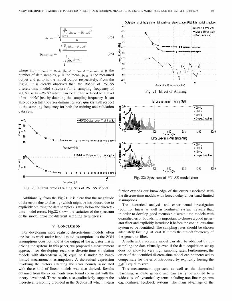
ARXIV PREPRINT: THE ARTICLE IS PUBLISHED IN IEEE TRANS. INSTRUM. MEAS.VOL. 65, ISSUE: 3, MARCH 2016, DOI: 10.1109/TIM.2015.2508279 10
yrms =
√√√√ n∑n=1
(yval − ymod)2
n(25)
yrelative =
√n∑n=1
(yval−ymod)2
n√n∑n=1
(yval)2
n
, (26)
where yval = yval − µval, ymod = ymod − µmod, n is thenumber of data samples, µ is the mean, yval is the measuredoutput and ymod is the model output respectively. From theFig.20, it is clearly observed that, the RMSE of PNLSSdiscrete-time model structure for a sampling frequency of200Hz is ≈ −25dB which can be further reduced to a levelof ≈ −44dB just by doubling the sampling frequency. It canalso be seen that the error diminishes very quickly with respectto the sampling frequency for both the training and validationdata sets.
Fig. 20: Output error (Training Set) of PNLSS Model
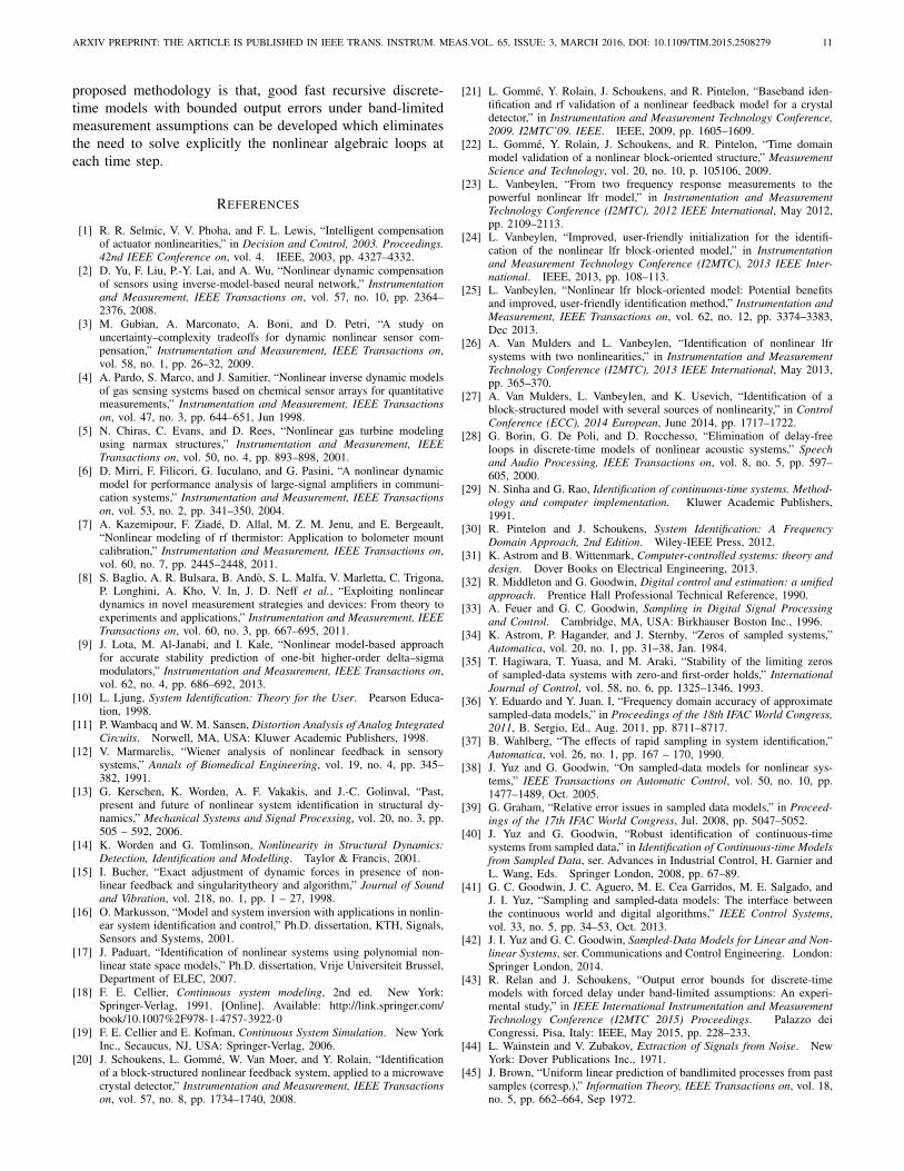
Additionally, from the Fig.21, it is clear that the magnitudeof the errors due to aliasing (which might be introduced due toexplicitly omitting the data samples) is way below the discrete-time model errors. Fig.22 shows the variation of the spectrumof the model error for different sampling frequencies.
V. CONCLUSION
For developing more realistic discrete-time models, oftenone has to work under band-limited assumptions as the ZOHassumptions does not hold at the output of the actuator that isdriving the system. In this paper, we proposed a measurementapproach for developing recursive discrete-time simulationmodels with direct-term gd(0) equal to 0 under the band-limited measurement assumptions. A theoretical expressioninvolving the factors affecting the error bounds associatedwith these kind of linear models was also derived. Resultsobtained from the experiments were found consistent with thetheory developed. These results also qualitatively support thetheoretical reasoning provided in the Section III which in-turn
Fig. 21: Effect of Aliasing
Fig. 22: Spectrum of PNLSS model error
further extends our knowledge of the errors associated withthe discrete-time models with forced delay under band-limitedassumptions.
The theoretical analysis and experimental investigation(both for linear as well as nonlinear system) reveals that,in order to develop good recursive discrete-time models withquantified error bounds, it is important to choose a good gener-ator filter and explicitly introduce it before the continuous-timesystem to be identified. The sampling rates should be chosenadequately fast, e.g. at least 10 times the cut-off frequency ofthe generator filter.
A sufficiently accurate model can also be obtained by up-sampling the data virtually, even if the data-acquisition set-updoes not allow for very high sampling rates. Furthermore, theorder of the identified discrete-time model can be increased tocompensate for the error introduced by explicitly forcing thegd(0) equal to zero.
This measurement approach, as well as the theoreticalreasoning, is quite generic and can easily be applied to awide class of dynamical systems including non-linear systemse.g. nonlinear feedback systems. The main advantage of the
ARXIV PREPRINT: THE ARTICLE IS PUBLISHED IN IEEE TRANS. INSTRUM. MEAS.VOL. 65, ISSUE: 3, MARCH 2016, DOI: 10.1109/TIM.2015.2508279 11
proposed methodology is that, good fast recursive discrete-time models with bounded output errors under band-limitedmeasurement assumptions can be developed which eliminatesthe need to solve explicitly the nonlinear algebraic loops ateach time step.
REFERENCES
[1] R. R. Selmic, V. V. Phoha, and F. L. Lewis, “Intelligent compensationof actuator nonlinearities,” in Decision and Control, 2003. Proceedings.42nd IEEE Conference on, vol. 4. IEEE, 2003, pp. 4327–4332.
[2] D. Yu, F. Liu, P.-Y. Lai, and A. Wu, “Nonlinear dynamic compensationof sensors using inverse-model-based neural network,” Instrumentationand Measurement, IEEE Transactions on, vol. 57, no. 10, pp. 2364–2376, 2008.
[3] M. Gubian, A. Marconato, A. Boni, and D. Petri, “A study onuncertainty–complexity tradeoffs for dynamic nonlinear sensor com-pensation,” Instrumentation and Measurement, IEEE Transactions on,vol. 58, no. 1, pp. 26–32, 2009.
[4] A. Pardo, S. Marco, and J. Samitier, “Nonlinear inverse dynamic modelsof gas sensing systems based on chemical sensor arrays for quantitativemeasurements,” Instrumentation and Measurement, IEEE Transactionson, vol. 47, no. 3, pp. 644–651, Jun 1998.
[5] N. Chiras, C. Evans, and D. Rees, “Nonlinear gas turbine modelingusing narmax structures,” Instrumentation and Measurement, IEEETransactions on, vol. 50, no. 4, pp. 893–898, 2001.
[6] D. Mirri, F. Filicori, G. Iuculano, and G. Pasini, “A nonlinear dynamicmodel for performance analysis of large-signal amplifiers in communi-cation systems,” Instrumentation and Measurement, IEEE Transactionson, vol. 53, no. 2, pp. 341–350, 2004.
[7] A. Kazemipour, F. Ziade, D. Allal, M. Z. M. Jenu, and E. Bergeault,“Nonlinear modeling of rf thermistor: Application to bolometer mountcalibration,” Instrumentation and Measurement, IEEE Transactions on,vol. 60, no. 7, pp. 2445–2448, 2011.
[8] S. Baglio, A. R. Bulsara, B. Ando, S. L. Malfa, V. Marletta, C. Trigona,P. Longhini, A. Kho, V. In, J. D. Neff et al., “Exploiting nonlineardynamics in novel measurement strategies and devices: From theory toexperiments and applications,” Instrumentation and Measurement, IEEETransactions on, vol. 60, no. 3, pp. 667–695, 2011.
[9] J. Lota, M. Al-Janabi, and I. Kale, “Nonlinear model-based approachfor accurate stability prediction of one-bit higher-order delta–sigmamodulators,” Instrumentation and Measurement, IEEE Transactions on,vol. 62, no. 4, pp. 686–692, 2013.
[10] L. Ljung, System Identification: Theory for the User. Pearson Educa-tion, 1998.
[11] P. Wambacq and W. M. Sansen, Distortion Analysis of Analog IntegratedCircuits. Norwell, MA, USA: Kluwer Academic Publishers, 1998.
[12] V. Marmarelis, “Wiener analysis of nonlinear feedback in sensorysystems,” Annals of Biomedical Engineering, vol. 19, no. 4, pp. 345–382, 1991.
[13] G. Kerschen, K. Worden, A. F. Vakakis, and J.-C. Golinval, “Past,present and future of nonlinear system identification in structural dy-namics,” Mechanical Systems and Signal Processing, vol. 20, no. 3, pp.505 – 592, 2006.
[14] K. Worden and G. Tomlinson, Nonlinearity in Structural Dynamics:Detection, Identification and Modelling. Taylor & Francis, 2001.
[15] I. Bucher, “Exact adjustment of dynamic forces in presence of non-linear feedback and singularitytheory and algorithm,” Journal of Soundand Vibration, vol. 218, no. 1, pp. 1 – 27, 1998.
[16] O. Markusson, “Model and system inversion with applications in nonlin-ear system identification and control,” Ph.D. dissertation, KTH, Signals,Sensors and Systems, 2001.
[17] J. Paduart, “Identification of nonlinear systems using polynomial non-linear state space models,” Ph.D. dissertation, Vrije Universiteit Brussel,Department of ELEC, 2007.
[18] F. E. Cellier, Continuous system modeling, 2nd ed. New York:Springer-Verlag, 1991. [Online]. Available: http://link.springer.com/book/10.1007%2F978-1-4757-3922-0
[19] F. E. Cellier and E. Kofman, Continuous System Simulation. New YorkInc., Secaucus, NJ, USA: Springer-Verlag, 2006.
[20] J. Schoukens, L. Gomme, W. Van Moer, and Y. Rolain, “Identificationof a block-structured nonlinear feedback system, applied to a microwavecrystal detector,” Instrumentation and Measurement, IEEE Transactionson, vol. 57, no. 8, pp. 1734–1740, 2008.
[21] L. Gomme, Y. Rolain, J. Schoukens, and R. Pintelon, “Baseband iden-tification and rf validation of a nonlinear feedback model for a crystaldetector,” in Instrumentation and Measurement Technology Conference,2009. I2MTC’09. IEEE. IEEE, 2009, pp. 1605–1609.
[22] L. Gomme, Y. Rolain, J. Schoukens, and R. Pintelon, “Time domainmodel validation of a nonlinear block-oriented structure,” MeasurementScience and Technology, vol. 20, no. 10, p. 105106, 2009.
[23] L. Vanbeylen, “From two frequency response measurements to thepowerful nonlinear lfr model,” in Instrumentation and MeasurementTechnology Conference (I2MTC), 2012 IEEE International, May 2012,pp. 2109–2113.
[24] L. Vanbeylen, “Improved, user-friendly initialization for the identifi-cation of the nonlinear lfr block-oriented model,” in Instrumentationand Measurement Technology Conference (I2MTC), 2013 IEEE Inter-national. IEEE, 2013, pp. 108–113.
[25] L. Vanbeylen, “Nonlinear lfr block-oriented model: Potential benefitsand improved, user-friendly identification method,” Instrumentation andMeasurement, IEEE Transactions on, vol. 62, no. 12, pp. 3374–3383,Dec 2013.
[26] A. Van Mulders and L. Vanbeylen, “Identification of nonlinear lfrsystems with two nonlinearities,” in Instrumentation and MeasurementTechnology Conference (I2MTC), 2013 IEEE International, May 2013,pp. 365–370.
[27] A. Van Mulders, L. Vanbeylen, and K. Usevich, “Identification of ablock-structured model with several sources of nonlinearity,” in ControlConference (ECC), 2014 European, June 2014, pp. 1717–1722.
[28] G. Borin, G. De Poli, and D. Rocchesso, “Elimination of delay-freeloops in discrete-time models of nonlinear acoustic systems,” Speechand Audio Processing, IEEE Transactions on, vol. 8, no. 5, pp. 597–605, 2000.
[29] N. Sinha and G. Rao, Identification of continuous-time systems. Method-ology and computer implementation. Kluwer Academic Publishers,1991.
[30] R. Pintelon and J. Schoukens, System Identification: A FrequencyDomain Approach, 2nd Edition. Wiley-IEEE Press, 2012.
[31] K. Astrom and B. Wittenmark, Computer-controlled systems: theory anddesign. Dover Books on Electrical Engineering, 2013.
[32] R. Middleton and G. Goodwin, Digital control and estimation: a unifiedapproach. Prentice Hall Professional Technical Reference, 1990.
[33] A. Feuer and G. C. Goodwin, Sampling in Digital Signal Processingand Control. Cambridge, MA, USA: Birkhauser Boston Inc., 1996.
[34] K. Astrom, P. Hagander, and J. Sternby, “Zeros of sampled systems,”Automatica, vol. 20, no. 1, pp. 31–38, Jan. 1984.
[35] T. Hagiwara, T. Yuasa, and M. Araki, “Stability of the limiting zerosof sampled-data systems with zero-and first-order holds,” InternationalJournal of Control, vol. 58, no. 6, pp. 1325–1346, 1993.
[36] Y. Eduardo and Y. Juan. I, “Frequency domain accuracy of approximatesampled-data models,” in Proceedings of the 18th IFAC World Congress,2011, B. Sergio, Ed., Aug. 2011, pp. 8711–8717.
[37] B. Wahlberg, “The effects of rapid sampling in system identification,”Automatica, vol. 26, no. 1, pp. 167 – 170, 1990.
[38] J. Yuz and G. Goodwin, “On sampled-data models for nonlinear sys-tems,” IEEE Transactions on Automatic Control, vol. 50, no. 10, pp.1477–1489, Oct. 2005.
[39] G. Graham, “Relative error issues in sampled data models,” in Proceed-ings of the 17th IFAC World Congress, Jul. 2008, pp. 5047–5052.
[40] J. Yuz and G. Goodwin, “Robust identification of continuous-timesystems from sampled data,” in Identification of Continuous-time Modelsfrom Sampled Data, ser. Advances in Industrial Control, H. Garnier andL. Wang, Eds. Springer London, 2008, pp. 67–89.
[41] G. C. Goodwin, J. C. Aguero, M. E. Cea Garridos, M. E. Salgado, andJ. I. Yuz, “Sampling and sampled-data models: The interface betweenthe continuous world and digital algorithms,” IEEE Control Systems,vol. 33, no. 5, pp. 34–53, Oct. 2013.
[42] J. I. Yuz and G. C. Goodwin, Sampled-Data Models for Linear and Non-linear Systems, ser. Communications and Control Engineering. London:Springer London, 2014.
[43] R. Relan and J. Schoukens, “Output error bounds for discrete-timemodels with forced delay under band-limited assumptions: An experi-mental study,” in IEEE International Instrumentation and MeasurementTechnology Conference (I2MTC 2015) Proceedings. Palazzo deiCongressi, Pisa, Italy: IEEE, May 2015, pp. 228–233.
[44] L. Wainstein and V. Zubakov, Extraction of Signals from Noise. NewYork: Dover Publications Inc., 1971.
[45] J. Brown, “Uniform linear prediction of bandlimited processes from pastsamples (corresp.),” Information Theory, IEEE Transactions on, vol. 18,no. 5, pp. 662–664, Sep 1972.

ARXIV PREPRINT: THE ARTICLE IS PUBLISHED IN IEEE TRANS. INSTRUM. MEAS.VOL. 65, ISSUE: 3, MARCH 2016, DOI: 10.1109/TIM.2015.2508279 12
[46] W. Splettstsser, “On the prediction of band-limited signals from pastsamples,” Information Sciences, vol. 28, no. 2, pp. 115 – 130, 1982.
[47] A. Papoulis, “A note on the predictability of band-limited processes,”Proceedings of the IEEE, vol. 73, no. 8, pp. 1332–1333, Aug 1985.
[48] F. Marvasti, “Comments on ”a note on the predictability of band-limitedprocesses”,” Proceedings of the IEEE, vol. 74, no. 11, pp. 1596–1596,Nov 1986.
[49] J. Brown, J.L., “On the prediction of a band-limited signal from pastsamples,” Proceedings of the IEEE, vol. 74, no. 11, pp. 1596–1598, Nov1986.
[50] F. J. Beutler, “Sampling theorems and bases in a hilbert space,” Infor-mation and Control, vol. 4, no. 23, pp. 97 – 117, 1961.
[51] F. Kuo and J. Kaiser, System analysis by digital computer. Wiley, 1966.[52] A. Oppenheim and R. Schafer, Discrete-Time Signal Processing: Pear-
son New International Edition. Pearson Education, Limited, 2013.[53] A. Papoulis, The Fourier Integral and Its Applications. Papoulis.
McGraw-Hill, 1962.[54] W. F. Mecklenbrauker, “Remarks on and correction to the impulse in-
variant method for the design of IIR digital filters,” Signal Processing,vol. 80, no. 8, pp. 1687 – 1690, 2000.
[55] L. Jackson, “A correction to impulse invariance,” Signal ProcessingLetters, IEEE, vol. 7, no. 10, pp. 273–275, Oct 2000.
[56] E. Eitelberg, “Convolution invariance and corrected impulse invariance,”Signal Processing, vol. 86, no. 5, pp. 1116 – 1120, 2006.
[57] S. R. Nelatury, “Additional correction to the impulse invariance methodfor the design of IIR digital filters,” Digital Signal Processing, vol. 17,no. 2, pp. 530 – 540, 2007.
[58] D. Swaroop and D. Neimann, “On the impulse response of lti systems,”in American Control Conference, 2001. Proceedings of the 2001, vol. 1,2001, pp. 523–528 vol.1.
[59] J. Schoukens, J. Nemeth, P. Crama, Y. Rolain, and R. Pintelon, “Fastapproximate identification of nonlinear systems,” Automatica, vol. 39,no. 7, pp. 1267 – 1274, 2003.
[60] J. Paduart, L. Lauwers, J. Swevers, K. Smolders, J. Schoukens, andR. Pintelon, “Identification of nonlinear systems using polynomialnonlinear state space models,” Automatica, vol. 46, no. 4, pp. 647 –656, 2010.
Related Documents