Recurrent neural networks for solving second-order cone programs

Neurocomputing 74 (2011) 3646–3653

Contents lists available at ScienceDirect

Neurocomputing

0925-23

doi:10.1

� Corr

Theoret

E-m

(J.-S. Ch1 Th

Taiwan

journal homepage: www.elsevier.com/locate/neucom

Recurrent neural networks for solving second-order cone programs

Chun-Hsu Ko a, Jein-Shan Chen b,1,�, Ching-Yu Yang b

a Department of Electrical Engineering, I-Shou University, Kaohsiung County 840, Taiwanb Department of Mathematics, National Taiwan Normal University, Taipei 11677, Taiwan

a r t i c l e i n f o

Article history:

Received 6 January 2011

Received in revised form

1 June 2011

Accepted 14 July 2011

Communicated by Y. Liuneural networks. We propose two kinds of neural networks with the different SOCCP functions. The

Available online 10 August 2011

Keywords:

SOCP

Neural network

Merit function

Fischer–Burmeister function

Cone projection function

Lyapunov stable

12/$ - see front matter & 2011 Elsevier B.V. A

016/j.neucom.2011.07.009

esponding author. Member of Mathematics

ical Sciences, Taipei Office.

ail addresses: [email protected] (C.-H. Ko), jsch

en), [email protected] (C.-Y. Yang).

e author’s work is partially supported by

.

a b s t r a c t

This paper proposes using the neural networks to efficiently solve the second-order cone programs

(SOCP). To establish the neural networks, the SOCP is first reformulated as a second-order cone

complementarity problem (SOCCP) with the Karush–Kuhn–Tucker conditions of the SOCP. The SOCCP

functions, which transform the SOCCP into a set of nonlinear equations, are then utilized to design the

first neural network uses the Fischer–Burmeister function to achieve an unconstrained minimization

with a merit function. We show that the merit function is a Lyapunov function and this neural network

is asymptotically stable. The second neural network utilizes the natural residual function with the cone

projection function to achieve low computation complexity. It is shown to be Lyapunov stable and

converges globally to an optimal solution under some condition. The SOCP simulation results

demonstrate the effectiveness of the proposed neural networks.

& 2011 Elsevier B.V. All rights reserved.

1. Introduction

Second-order cone program (SOCP) has been widely applied inengineering optimization [1]. It requires solving the optimizationproblem subject to the linear equality and second-order coneinequality constraints [2]. Numerical approaches such as theinterior-point method [1] or the merit function method [3] caneffectively solve the SOCP. However, many engineering dynamicsystems, such as force analysis in robot grasping [1,4] and controlapplications [5,6], require the real-time SOCP solutions. As aresult, efficient approaches for solving the real-time SOCP areneeded. Prior research [7–18] indicates that the neural networkscan be used to solve various optimization problems. Furthermore,the neural networks based on circuit implementation exhibit thereal-time processing ability. We consider that it is appropriate toutilize the neural networks for efficiently solving the SOCPproblems.

The recurrent neural network was introduced by Hopfield andTank [7] for solving linear programming problems. Kennedy andChua [8] proposed an extended neural network for solving non-linear convex programming problems thereafter, while their

ll rights reserved.

Division, National Center for

[email protected]

National Science Council of

approach involves the penalty parameter which affects the neuralnetwork accuracy. To find the exact solutions, more neuralnetworks for optimization have been further developed. Amongthem, the primal-dual neural network [9–11] with the globalstability is proposed for providing the exact solutions of the linearand quadratic programming problems. The projection neuralnetwork, developed by Xia and Wang [12,14,15], was proposedto efficiently solve many optimization problems and variationalinequalities. Since the SOCP is a nonlinear convex problem, bothprimal-dual neural network [16] and projection neural network[17] can be used to provide the SOCP solution. However, theyrequire many state variables, leading to high model complexity. Itthus motivates the development of more compact neuralnetworks for SOCP.

The SOCP can be solved by analyzing its Karush–Kuhn–Tucker(KKT) optimality conditions which leads to the second-order conecomplementarity problem (SOCCP) [3,19,20]. The approaches[3,20] based on the SOCCP functions, such as Fischer–Burmeister(FB) and natural residual functions, can be further utilized forsolving the SOCCP. In the merit function approach [3], anunconstrained smooth minimization with the FB function isachieved in finding the SOCCP solution. On the other hand, thesemi-smooth approach [20] uses the natural residual functionwith the cone projection (CP) function to reformulate the SOCCPas a set of nonlinear equations and then apply the non-smoothNewton method to obtain the solution. Previous studies havedemonstrated the feasibility of these SOCCP functions in solvingthe SOCP problems. We also use them in our neural network

C.-H. Ko et al. / Neurocomputing 74 (2011) 3646–3653 3647

design. In this paper, we propose two novel neural networks forefficiently solving the SOCP problems. One is based on thegradient of the smooth merit function derived from the FBfunction [18]. The other is an extended projection neural networkby replacing the scalar projection function [12,14,15] with the CPfunction. These neural networks are with less state variables thanthose previously proposed [16,17] for solving the SOCP. Further-more, they are shown to be stable and globally convergent to theSOCP solutions.

This paper is organized as follows. Section 2 introduces thesecond-order cone program and its SOCCP formulation. In Section3, the neural network based on the Fischer–Burmeister function isproposed and analyzed. In Section 4, the second neural networkbased on the cone projection function is proposed. Its globalstability is also verified. In Section 5, several SOCP examples arepresented to demonstrate the effectiveness of the proposedneural networks. Finally, the conclusions are given in Section 6.

2. Problem formulation

In this section, we introduce the second-order cone programand reformulate it as a second-order cone complementarityproblem. The second-order cone program is in the form of

minimize f ðxÞ

subject to Ax¼ b, xAK : ð1Þ

Here f : Rn-R is a nonlinear continuously differentiable func-tion, AARm�n is a full row rank matrix, bARm is a vector, and K isa Cartesian product of second-order cones (or Lorentz cones),expressed as

K ¼ Kn1 � Kn2 � � � � � KnN , ð2Þ

where N,n1, . . . ,nN Z1,n1þ � � � þnN ¼ n, and

Kni :¼ fðxi1,xi2, . . . ,xiniÞT ARni 9 Jðxi2, . . . ,xini

ÞJrxi1g

with J � J denoting the Euclidean norm and K1 the set of non-negative reals Rþ . A special case of Eq. (2) is K ¼Rn

þ , namely thenonnegative orthant in Rn, which corresponds to N¼n andn1 ¼ � � � ¼ nN ¼ 1. When f is linear, i.e., f ¼ cT x with cARn, SOCP(1) reduces to the following linear SOCP:

minimize cT x

subject to Ax¼ b, xAK : ð3Þ

The KKT optimality conditions for (1) are given by

rf ðxÞ�AT y�l¼ 0,

xTl¼ 0, xAK , lAK ,

Ax¼ b,

8><>: ð4Þ

where yARm and lARn. When f is convex, these conditions aresufficient for optimality. It also can be written as

xT ðrf ðxÞ�AT yÞ ¼ 0, xAK , rf ðxÞ�AT yAK ,

Ax¼ b:

(ð5Þ

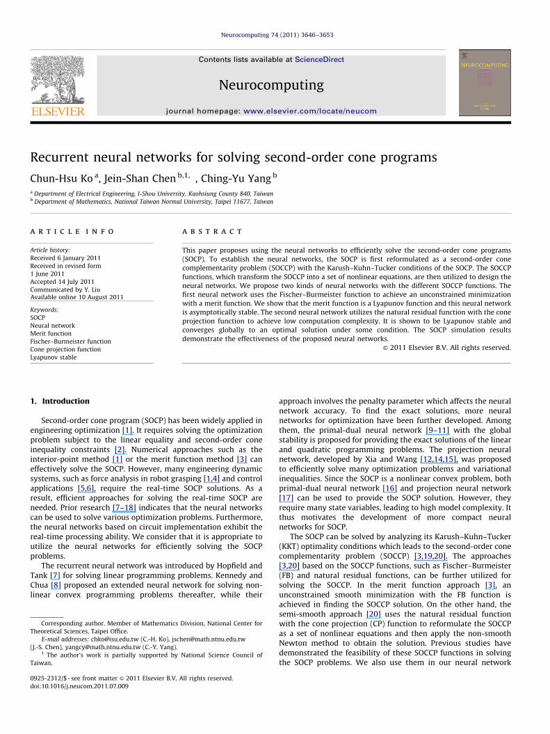
By solving the system (5), we may obtain a primal-dual optimalsolution of SOCP (1). Note that system (5) involves the SOCCP. Toefficiently solve it, we propose using the neural networkapproaches with the FB function and CP function, respectively,described below.

Fig. 1. Block diagram of the proposed neural network with FB function.

3. Neural network design with Fischer–Burmeister function

It is known that the merit function approach [3] can be usedfor solving system (5). Motivated by this approach, we propose a

neural network with the Fischer–Burmeister function to find theminimal of the merit function and study its global stability.

In [3], system (5) is shown to be equivalent to an uncon-strained smooth minimization problem via the merit functionapproach, described as

min Eðx,yÞ ¼CFBðx,rf ðxÞ�AT yÞþ12JAx�bJ2, ð6Þ

where Eðx,yÞ is a merit function, CFBðx,yÞ ¼ 12

PNi ¼ 1 JfFBðxi,yiÞJ

2,

x¼ ðx1, . . . ,xNÞT , y¼ ðy1, . . . ,yNÞ

T ARn1 � � � � �RnN , and fFB is theFischer–Burmeister function defined as

fFBðxi,yiÞ :¼ ðx2i þy2

i Þ1=2�xi�yi: ð7Þ

Based on the gradient of the objective Eðx,yÞ in minimizationproblem (6), we propose the first neural network for solving theSOCP, with the following dynamic equation:

d

dt

x

y

!¼ r

�rxEðx,yÞ

�ryEðx,yÞ

!, ð8Þ

where r is a positive scaling factor and

rxEðx,yÞ ¼rxCFBðx,rf ðxÞ�AT yÞ

þr2f ðxÞ � ryCFBðx,rf ðxÞ�AT yÞþAT ðAx�bÞ,

ryEðx,yÞ ¼�A � ryCFBðx,rf ðxÞ�AT yÞ:

8>><>>: ð9Þ

For linear SOCP (3), the above equations reduce to

rxEðx,yÞ ¼rxCFBðx,c�AT yÞþAT ðAx�bÞ,

ryEðx,yÞ ¼�A � ryCFBðx,c�AT yÞ:

(ð10Þ

Note that the Jordan product [3] is required for calculating rxCFB

and ryCFB which are introduced in Appendix. And, the dynamic

equation (8) can be realized by a recurrent neural network withFB function as shown in Fig. 1. The circuit for the neural network

realization requires nþm integrators, n processors for rf ðxÞ, n2

processors for r2f ðxÞ, n processors for rxCFB, m processors for

ryCFB, 4mn connection weights and some summers. Further-

more, the neural network (8) is asymptotically stable, as provenin the following theorem.

C.-H. Ko et al. / Neurocomputing 74 (2011) 3646–36533648

Theorem 3.1. If un ¼ ðxn,ynÞ is an isolated equilibrium point of

neural network (8), then un ¼ ðxn,ynÞ is asymptotically stable for (8).

Proof. We assume that un ¼ ðxn,ynÞ is an isolated equilibriumpoint of neural network (8) over a neighborhood OnDRn of un

such that rEðxn,ynÞ ¼ 0 and rEðx,yÞa0, 8ðx,yÞAOn\fðxn,ynÞg. Firstwe show that Eðx,yÞ is a Lyapunov function for un at On. Since

ryEðxn,ynÞ ¼�A � ryCFBðxn,rf ðxnÞ�AT ynÞ ¼ 0,

from Lemma 3 and Proposition 1 of [3], we have

rxCFBðxn,rf ðxnÞ�AT ynÞ ¼ryCFBðx

n,rf ðxnÞ�AT ynÞ ¼ 0:

Moreover, from Proposition 1 of [3], this says

CFBðxn,rf ðxnÞ�AT ynÞ ¼ 0:

Then from Eq. (9),

rxEðxn,ynÞ ¼rxCFBðxn,rf ðxnÞ�AT ynÞ

þr2f ðxnÞ � ryCFBðxn,rf ðxnÞ�AT ynÞ

þAT ðAxn�bÞ ¼ 0,

which implies that AT ðAxn�bÞ ¼ 0. Because AARm�n is a full row

rank matrix, we must have Axn�b¼ 0, which yields

Eðxn,ynÞ ¼CFBðxn,rf ðxnÞ�AT ynÞþ1

2JAxn�bJ2

¼ 0:

Next, we claim that Eðx,yÞ40, 8ðx,yÞAOn\fðxn,ynÞg. If not, there isan ðx,yÞAOn\fðxn,ynÞg such that Eðx,yÞ ¼ 0, this says thatCFBðx,rf ðxÞ�AT yÞ ¼ 0 and Ax¼b, then rxEðx,yÞ ¼ 0 andryEðx,yÞ ¼ 0. Hence, (x,y) is an equilibrium point of neural net-work (8), contradicting with that un ¼ ðxn,ynÞ is an isolate equili-brium point. Finally,

dEðxðtÞ,yðtÞÞ

dt¼ ½rðxðtÞ,yðtÞÞEðxðtÞ,yðtÞÞ�

T ð�rrðxðtÞ,yðtÞÞEðxðtÞ,yðtÞÞÞ

¼ �rJrðxðtÞ,yðtÞÞEðxðtÞ,yðtÞÞJ2r0:

Therefore, the function Eðx,yÞ is a Lyapunov function for neuralnetwork (8) over the set On. Since un ¼ ðxn,ynÞ is an isolatedequilibrium point of neural network (8), we have

dEðxðtÞ,yðtÞÞ

dto0, 8ðxðtÞ,yðtÞÞAOn\fðx

n,ynÞg:

Thus, un is asymptotically stable for neural network (8). &

4. Neural network design with cone projection function

In this section, we propose another neural network associatedwith the cone projection function to solve system (5) for obtain-ing the SOCP solution and study its stability. In fact, from [24,Proposition 3.3], we know that such cone projection onto K has aspecial formula given as

PK ðzÞ ¼ ½l1ðzÞ�þuð1Þz þ½l2ðzÞ�þuð2Þz ,

where ½��þ means the scalar projection, l1ðzÞ, l2ðzÞ and uð1Þz , uð2Þz arethe spectral values and the associated spectral vectors ofz¼ ðz1,z2ÞAR�Rn�1, respectively, given by

liðzÞ ¼ z1þð�1ÞiJz2J,

uðiÞz ¼1

21,ð�1Þi

z2

Jz2J

� �,

8><>:for i¼1,2. The CP function PK(z) has the following property, calledprojection theorem [21], which is useful in our subsequentanalysis.

Property 4.1. Let K be a nonempty closed convex subset of Rn. Then,for each zARn, PK(z) is the unique vector zAK satisfying

ðy�zÞT ðz�zÞr0, 8yAK.

Employing the natural residual function with the CP function[19,20], system (5) can be equivalently written as

x�PK ðx�rf ðxÞþAT yÞ ¼ 0,

Ax�b¼ 0,

(ð11Þ

where x¼ ðx1, . . . ,xNÞT ARn1 � � � � �RnN with xi ¼ ðxi1,xi2, . . . ,xini

ÞT ,

i¼ 1, . . . ,N, and PK ðxÞ ¼ ½PK ðx1Þ, . . . ,PK ðxNÞ�T .

Based on the equivalent formulation in (11) and employing theideas for networks used in [12,13], we consider the second neuralnetwork for solving the SOCP, with the following dynamicequations:

d

dt

x

y

!¼ r

�xþPK ðx�rf ðxÞþAT yÞ

�Axþb

!, ð12Þ

where r is a positive scaling factor. The dynamic can be realizedby a recurrent neural network with the cone projection functionas shown in Fig. 2. The circuit for the neural network realizationrequires nþm integrators, n processors for rf ðxÞ, N processors forcone projection mapping PK, 2mn connection weights and somesummers. Compared with the first neural network in (8), thesecond neural network (12) dose not require to calculate r2f ðxÞ,resulting in lower model complexity.

To analyze the stability of the neural network in Eq. (12), wefirst give three lemmas and one proposition.

Lemma 4.1. Let F(u) be defined as

FðuÞ :¼ Fðx,yÞ :¼�xþPK ðx�rf ðxÞþAT yÞ

�Axþb

!: ð13Þ

Then, F(u) is semi-smooth. Moreover, F(u) is strongly semi-smooth if

r2f ðxÞ is locally Lipschitz continuous.

Proof. This is an immediate consequence of [20, Theorem 1]. &

Proposition 4.1. For any initial point u0 ¼ ðx0,y0Þ where

x0 :¼ xðt0ÞAK , there exists a unique solution uðtÞ ¼ ðxðtÞ,yðtÞÞ for

neural network (12). Moreover, xðtÞAK.

Proof. For simplicity, we assume K ¼ Kn. The analysis can becarried over to the general case where K is the Cartesian productof second-order cones. From Lemma 4.1, FðuÞ :¼ Fðx,yÞ is semi-smooth and Lipschitz continuous. Thus, there exists a uniquesolution uðtÞ ¼ ðxðtÞ,yðtÞÞ for neural network (12). Therefore, itremains to show that xðtÞAKn. For convenience, we denotexðtÞ :¼ ðx1ðtÞ,x2ðtÞÞAR�Rn�1. To complete the proof, we need toverify two things: (i) x1ðtÞZ0 and (ii) Jx2ðtÞJrx1ðtÞ. First, from(12), we have

dx

dtþrxðtÞ ¼ rPK ðx�rf ðxÞþAT yÞ:

The solution of the first-order ordinary differential equationabove is

xðtÞ ¼ e�rðt�t0Þxðt0Þþre�rt

Z t

t0

ersPK ðx�rf ðxÞþAT yÞds:

If we let xðt0Þ :¼ ðx1ðt0Þ,x2ðt0ÞÞAR�Rn�1 and denote zðtÞ :¼ðz1ðt0Þ,z2ðt0ÞÞ as the term PK ðx�ðrf ðxÞ�AT yÞÞ, which leads to

x1ðtÞ ¼ e�rðt�t0Þx1ðt0Þþre�rt

Z t

t0

ersz1ðsÞds,

x2ðtÞ ¼ e�rðt�t0Þx2ðt0Þþre�rt

Z t

t0

ersz2ðsÞds:

Due to both x0ðtÞ and z(t) belong to Kn, there have x1ðt0ÞZ0,Jx2ðt0ÞJrx1ðt0Þ and z1ðtÞZ0, Jz2ðtÞJrz1ðtÞ. Therefore, x1ðtÞZ0since both terms in the right-hand side are nonnegative.

Fig. 2. Block diagram of the proposed neural network with CP function.

C.-H. Ko et al. / Neurocomputing 74 (2011) 3646–3653 3649

In addition,

Jx2ðtÞJre�rðt�t0ÞJx2ðt0ÞJþre�rt

Z t

t0

ersJz2ðsÞJds

re�rðt�t0Þx1ðt0Þþre�rt

Z t

t0

ersz1ðsÞds¼ x1ðtÞ,

which implies that xðtÞAKn. &

Lemma 4.2. Let H(u) be defined as

HðuÞ :¼ Hðx,yÞ :¼rf ðxÞ�AT y

Ax�b

!: ð14Þ

Then, H is a monotone function if f is a convex function. Moreover,rHðuÞ is positive semi-definite if and only if r2f ðxÞ is positive semi-definite.

Proof. Let u¼ ðx,yÞ and ~u ¼ ð ~x, ~yÞ. Then, the monotonicity of H

holds since

ðu� ~uÞT ðHðuÞ�Hð ~uÞÞ ¼ ðx� ~xÞT ðrf ðxÞ�rf ð ~xÞÞ�ðx� ~xÞT ðAT ðy� ~yÞÞ

þðy� ~yÞT ðAðx� ~xÞÞ ¼ ðx� ~xÞT ðrf ðxÞ�rf ð ~xÞÞZ0,

where the last inequality is due to the convexity of f(x), see [22,Theorem 3.4.5]. Furthermore, we observe that

rHðuÞ ¼r2f ðxÞ �AT

A 0

" #:

Thus, we have

uTrHðuÞu¼ ½xT yT �r

2f ðxÞ �AT

A 0

" #x

y

" #¼ xTr

2f ðxÞx,

which indicates that the positive semi-definiteness of rHðuÞ isequivalent to the positive semi-definiteness of r2f ðxÞ. &

Lemma 4.3. Let F(u) and H(u) be defined as in (13) and (14),respectively. Also, let un ¼ ðxn,ynÞ be an equilibrium point of neural

network (12) with xn being an optimal solution of SOCP. Then, the

following inequalities hold:

ðFðuÞþu�unÞTð�FðuÞ�HðuÞÞZ0: ð15Þ

Proof. First, we denote l :¼ rf ðxÞ�AT y. Then, we obtain

ðFðuÞþu�unÞTð�FðuÞ�HðuÞÞ

C.-H. Ko et al. / Neurocomputing 74 (2011) 3646–36533650

¼�xþPK ðx�lÞþðx�xnÞ

ð�AxþbÞþðy�ynÞ

" #Tx�PK ðx�lÞ�lðAx�bÞ�ðAx�bÞ

" #

¼�xnþPK ðx�lÞð�AxþbÞþðy�ynÞ

" #Tðx�lÞ�PK ðx�lÞ

0

� �

¼�ðxn�PK ðx�lÞÞT ððx�lÞ�PK ðx�lÞÞ:

Since xnAK , applying Property 4.1 gives

ðxn�PK ðx�lÞÞT ððx�lÞ�PK ðx�lÞÞr0:

Thus, inequality (15) is proved. &

We now investigate the stability and convergence issues ofneural network (12). First, we analyze the behavior of the solutiontrajectory of neural network (12) including existence and con-vergence. We then establish two kinds of stability for an isolatedequilibrium point.

We know that every solution un to SOCP is an equilibriumpoint of neural network (12). If further un is an isolated equili-brium point of neural network (12), we show that un is Lyapunovstable.

Theorem 4.1. If f is convex and twice differentiable, then the

solution of neural network (12), with initial point u0 ¼ ðx0,y0Þ where

x0AK , is Lyapunov stable. Moreover, the solution trajectory of neural

network (12) is extendable to the global existence.

Proof. Again, for simplicity, we assume K ¼ Kn. From Proposition4.1, there exists a unique solution uðtÞ ¼ ðxðtÞ,yðtÞÞ for neuralnetwork (12) and xðtÞAKn. Let un ¼ ðxn,ynÞ be an equilibrium pointof neural network (12) with xn being an optimal solution of SOCP.We define a Lyapunov function as below:

EðuÞ :¼ Eðx,yÞ :¼ �HðuÞT FðuÞ�12 JFðuÞJ2

þ12Ju�unJ2, ð16Þ

where F(u) and H(u) are given as in (13) and (14), respectively.From [23, Theorem 3.2], we know that E is continuously differ-entiable with

rEðuÞ ¼HðuÞ�½rHðuÞ�I�FðuÞþðu�unÞ:

It is also trivial that EðunÞ ¼ 0. Then, we have

dEðuðtÞÞ

dt¼rEðuðtÞÞT

du

dt¼ fHðuÞ�½rHðuÞ�I�FðuÞþðu�unÞgTrFðuÞ

¼ rf½HðuÞþðu�unÞ�T FðuÞþJFðuÞJ2�FðuÞTrHðuÞFðuÞg:

Hence, inequality (15) in Lemma 4.3 implies

ðHðuÞþu�unÞT FðuÞr�HðuÞT ðu�unÞ�JFðuÞJ2,

which yields

dEðuðtÞÞ

dtrrf�HðuÞT ðu�unÞ�FðuÞTrHðuÞFðuÞg

¼ rf�HðunÞTðu�unÞ�ðHðuÞ�HðunÞÞ

Tðu�unÞ

�FðuÞTrHðuÞFðuÞg: ð17Þ

On the other hand, we know that

ðFðunÞþun�uÞT ð�FðunÞ�HðunÞÞ ¼ �ðx�PK ðxn�ln

ÞÞTððxn�ln

Þ�PK ðxn�ln

ÞÞ:

Since xAKn, applying Property 4.1 gives

ðx�PK ðxn�ln

ÞÞTððxn�ln

Þ�PK ðxn�ln

ÞÞr0:

Thus, we have ðFðunÞþun�uÞT ð�FðunÞ�HðunÞÞZ0. Note thatFðunÞ ¼ 0, we therefore obtain �HðunÞ

Tðu�unÞ

T r0. Also the mono-tonicity of H implies �ðHðuÞ�HðunÞÞ

Tðu�unÞr0. In addition, f is

convex and twice differentiable if and only if r2f ðxÞ is positivesemidefinite and hence rH is positive semidefinite by Lemma 4.2,i.e., the second term �FðuÞTrHðuÞFðuÞr0. The above discussionslead to dEðuðtÞÞ=dtr0.

In order to obtain E(u) is a Lyapunov function and un is

Lyapunov stable, we will show the following inequality:

�HðuÞT FðuÞZJFðuÞJ2: ð18Þ

To see this, we first observe that

JFðuÞJ2þHðuÞT FðuÞ ¼ ðx�PK ðx�lÞÞT ððx�lÞ�PK ðx�lÞÞ:

Since xAK , applying Property 4.1 again, there holds

ðx�PK ðx�lÞÞT ððx�lÞ�PK ðx�lÞÞr0,

which yields the desired inequality (18). By combining Eq. (16)

and inequality (18), we have

EðuÞZ12 JFðuÞJ2

þ12Ju�unJ2,

which says EðuÞ40 if uaun. Hence E(u) is indeed a Lyapunov

function and un is Lyapunov stable. Moreover, it holds that

Eðu0ÞZEðuÞZ12Ju�unJ2 for tZt0, ð19Þ

which means the solution trajectory u(t) is bounded. Hence, it can

be extended to global existence. &

Theorem 4.2. Let un ¼ ðxn,ynÞ be an equilibrium point of (12) with

xn being an optimal solution of SOCP. If f is twice differentiable and

r2f ðxÞ is positive definite, the solution of neural network (12), with

initial point u0 ¼ ðx0,y0Þ where x0AK , is globally convergent to un

and has finite convergence time.

Proof. From (19), the level set

Lðu0Þ :¼ fu 9 EðuÞrEðu0Þg

is bounded. Then, the Invariant Set Theorem [25] implies thesolution trajectory u(t) converges to y as t-1 where y is thelargest invariant set in

P¼ uALðu0ÞdEðuðtÞÞ

dt¼ 0

������:

We will show that du=dt¼ 0 if and only if dEðuðtÞÞ=dt¼ 0 whichyields that u(t) converges globally to the equilibrium pointun ¼ ðxn,ynÞ. Suppose du=dt¼ 0, then it is clear that dEðuðtÞÞ=dt¼

rEðuÞT ðdu=dtÞ ¼ 0. Let u ¼ ðx,yÞAP which says dEðuðtÞÞ=dt¼ 0.From (17), we know that

dEðuðtÞÞ

dtrrf�ðHðuÞ�HðunÞÞ

Tðu�unÞ�FðuÞTrHðuÞFðuÞg:

Both terms inside the big parenthesis are nonpositive as shown inLemma 4.2, so ðHðuÞ�HðunÞÞ

Tðu�unÞ ¼ 0, FðuÞTrHðuÞFðuÞ ¼ 0, and

FðuÞTrHðuÞFðuÞ ¼ f�xþPK ðx�rf ðxÞþAT yÞgTr2f ðxÞf�x

þPK ðx�rf ðxÞþAT yÞg ¼ 0:

The condition of r2f ðxÞ being positive definite leads to

�xþPK ðx�rf ðxÞþAT yÞ ¼ 0,

which is equivalent to dx=dt¼ 0. On the other hand, similar to thearguments in Lemma 4.2, we have

ðu�unÞTðHðuÞ�HðunÞÞ ¼ ðx�xnÞ

Tðrf ðxÞ�rf ðxnÞÞ

¼ ðx�xnÞTr2f ðxsÞðx�xnÞ ¼ 0,

where xsA ½xn,x�. Again, the condition of r2f ðxsÞ being positivedefinite yields x ¼ xn. Hence dy=dt¼ 0 and therefore duðtÞ=dt¼ 0.From above, u(t) converges globally to the equilibrium pointun ¼ ðxn,ynÞ. Moreover, with Theorem 4.1 and following the samearguments as in [12, Theorem 2], the neural network (12) has finiteconvergence time. &

C.-H. Ko et al. / Neurocomputing 74 (2011) 3646–3653 3651

5. Simulations

To demonstrate the effectiveness of the proposed neural net-works, three illustrative SOCP problems are tested, described asbelow.

Example 5.1. Consider the nonlinear convex SOCP [20] given by

minimize exp ðx1�x3Þþ3ð2x1�x2Þ4þ

ffiffiffiffiffiffiffiffiffiffiffiffiffiffiffiffiffiffiffiffiffiffiffiffiffiffiffiffiffiffiffiffiffi1þð3x2þ5x3Þ

2q

subject to Ax¼ b, xAK3 � K2,

where

A¼4 6 3 �1 0

�1 7 �5 0 �1

� �and b¼

1

�2

� �:

This problem has an approximate solution xn ¼ ½0:2324,�0:07309,0:2206,0:153,0:153�T . We use the proposed neural net-works with the FB and CP functions, respectively, to solve theproblem with the trajectories obtained by them shown inFigs. 3 and 4. From the simulation results, we found that bothtrajectories are globally convergent to xn and the neural networkwith the CP function converged to xn quicker than that with the FB

0 0.05 0.1 0.15 0.2−0.2

0

0.2

0.4

0.6

0.8

1

Time (sec)

Traj

ecto

ries

of x

(t)

x1

x2

x3

x4, x5

Fig. 3. Transient behavior of the neural network with FB function in Example 5.1.

0 0.005 0.01 0.015 0.02 0.025 0.03−1

−0.5

0

0.5

1

1.5

2

2.5

3

Time (sec)

Traj

ecto

ries

of x

(t)

x1

x2

x3

x4, x5

Fig. 4. Transient behavior of the neural network with CP function in Example 5.1.

function. On the other hand, the neural network with the CP functionalso has lower model complexity than that with the FB function asmentioned in Section 4. Hence, the neural network with the CPfunction is preferable to the neural network with the FB functionwhen both can globally converge to the optimal solution.

Example 5.2. Consider the following linear SOCP given by

minimize x1þx2þx3þx4þx5þx6

subject to Ax¼ b, xAK3 � K3,

where

A¼

1 2 0 0 0 1

1 0 0 1 4 0

0 1 1 0 1 0

1 1 0 0 0 0

0 0 1 0 2 0

26666664

37777775

and b¼

9

20

6

4

8

26666664

37777775

This problem has an optimal solution xn ¼ ½3,1,2,5,3,4�T . Notethat, its objective function is convex and the Hessian matrixr2f ðxÞ is a zero matrix. Hence, the neural network with the FBfunction is asymptotically stable from Theorem 3.1 while theneural network with the CP function is Lyapunov stable fromTheorem 4.1. Figs. 5 and 6 display the trajectories obtained usingthe neural networks with the FB and CP functions, respectively.The simulation results show that both trajectories are convergentto xn. Coinciding with above results of Theorems 3.1 and 4.1, theneural network with the CP function yields the oscillatingtrajectory and has longer convergence time than the neuralnetwork with the FB function.

Example 5.3. Consider the grasping force optimization problemfor the multi-fingered robotic hand [1,4,17]. Its goal is to find theminimum grasping force for moving an object. For the robotic handwith m fingers, the optimization problem can be formulated as

minimize 12 f T f

subject toGf ¼�fext

Jðfi1,fi2ÞJrmfi3 ði¼ 1, . . . ,mÞ,

where f ¼ ½f11,f12, . . . ,fm3�T is the grasping force, G the grasping

transformation matrix, fext the time-varying external wrench, and mthe friction coefficient.

0 0.05 0.1 0.15 0.2 0.25 0.3 0.35 0.40

1

2

3

4

5

6

Time (sec)

Traj

ecto

ries

of x

(t)

x1, x5

x2

x3

x4

x6

Fig. 5. Transient behavior of the neural network with FB function in Example 5.2.

0 0.2 0.4 0.6 0.8 10

1

2

3

4

5

6

Time (sec)

Traj

ecto

ries

of x

(t)

x1, x5

x2

x3

x4

x6

Fig. 6. Transient behavior of the neural network with CP function in Example 5.2.

0 0.2 0.4 0.6 0.8 1−1

−0.5

0

0.5

1

1.5

2

Time (sec)

Gra

spin

g fo

rce

(N)

f11,f32

f12

f13

f21

f22

f23

f31

f33

Fig. 7. Grasping force obtained by using proposed neural networks in Example

5.3.

C.-H. Ko et al. / Neurocomputing 74 (2011) 3646–36533652

Letting ½xi1,xi2,xi3� ¼ ½mfi3,fi1,fi2�,i¼ 1, . . . ,m, and x¼ ½x11,x12, . . . ,

xm3�T , the problem can be reformulated as a nonlinear convex

SOCP. For the three-finger grasp example in [17], the robot hand

grasps a polyhedral with the grasp points ½0,1,0�T , ½1,0:5,0�T , and

½0,�1,0�T , and the robot hand moves along a vertical circulartrajectory of radius r with a constant velocity n. We reformulatethe example as

minimize 12 xT Qx

subject to Ax¼ b, xAK3 � K3 � K3, ð20Þ

where Q ¼ diagð1=m2,1,1,1=m2,1,1,1=m2,1,1Þ

A¼

0 0 1 �1=m 0 0 0 1 0

�1=m 0 0 0 0 �1 1=m 0 0

0 �1 0 0 �1 0 0 0 �1

0 �1 0 0 �0:5 0 0 0 1

0 0 0 0 1 0 0 0 0

0 0 �1 0:5=m 0 �1 0 1 0

26666666664

37777777775

and

b¼

0

�fc sin yðtÞMg�fc cos yðtÞ

0

0

0

2666666664

3777777775

,

where M is the mass of the polyhedral, g¼9.8 m/s2, fc ¼Mn2=r the

centripetal force, t the time, and y¼ nt=rA ½0,2p�. Note thatproblem (20) is a nonlinear convex SOCP and the matrix Q ispositive definite. We know from Theorems 3.1 and 4.2 that boththe proposed neural networks are globally convergent to theoptimal solution. Under the conditions M¼0.1 kg, r¼0.2 m,n¼ 0:4p m=s, and m¼ 0:6, the time-varying grasping forceobtained from the proposed neural networks is shown in Fig. 7.We found that the maximum grasping force occurs at the position

y¼ p (t¼0.5 s) which corresponds to the maximum downwardwrench. The simulation results demonstrate that the neuralnetworks are effective in the SOCP applications.

6. Conclusion

In this paper, we have proposed two neural networks forefficiently solving the SOCP. The first neural network is based ongradient of the merit function derived from the FB function andwas shown to be asymptotically stable. The second neural networkwith the CP function has low model complexity, and has beenshown to be Lyapunov stable and converge globally to the SOCPsolution under the positive definite condition of Hessian matrix ofthe objective function. The convergence of the neural networks hasbeen validated with the simulation results of the SOCP examples.When the second neural network with the CP functions yieldsoscillating trajectory, we can employ the neural network based onFB function instead, though it has higher model complexity. Theproposed neural networks are thus ready for the SOCP applications.

During the reviewing process of this paper, we published anotherpaper [26] which focuses on second-order cone constrained varia-tional inequality problem. Since the KKT conditions of second-ordercone programs can be recast as variational inequality problem, thepaper [26] indeed deals with a broader class of optimizationproblems. However, the two neural networks considered thereinare different from the two neural networks studied in this paper.More specifically, the FB method used in [26] is based on thesmoothed FB function while the one studied here is based on regularFB function; the CP method in [26] is based on a Lagrangian modelwhich is, even when it reduces to SOCP, not the same as the oneinvestigated here. Due to the essential difference, the assumptionsused to establish stability are also different. In view of this, it will bean interesting topic to do numerical comparison among these neuralnetworks for SOCP.

Acknowledgement

The work was supported by National Science Council ofTaiwan under the Grant NSC 97-2221-E-214-034.

Appendix

In this appendix, we introduce the Jordan product and itsproperties used in the neural network with the FB function, whichare needed when we write codes for simulations.

C.-H. Ko et al. / Neurocomputing 74 (2011) 3646–3653 3653

For any x¼ ðx1,x2ÞAR�Rn�1, their Jordan product is defined as

xJy¼ ðxT y,y1x2þx1y2Þ:

Their sum of square is calculated by

x2þy2 ¼ ðJxJ2þJyJ2,2x1x2þ2y1y2Þ:

The square root of x is

x1=2 ¼ s,x2

2s

�, s¼

ffiffiffiffiffiffiffiffiffiffiffiffiffiffiffiffiffiffiffiffiffiffiffiffiffiffiffiffiffiffiffiffiffiffiffiffiffiffiffiffi1

2ðx1þ

ffiffiffiffiffiffiffiffiffiffiffiffiffiffiffiffiffiffiffiffix2

1�Jx2J2

qÞ

rif x¼ 0, x1=2 ¼ 0

and the determinant of x is det ðxÞ ¼ x21�Jx2J

2. Furthermore, amatrix Lx is defined as

Lx ¼x1 xT

2

x2 x1I

" #,

and when detðxÞa0, Lx is invertible with

L�1x ¼

1

det ðxÞ

x1 �xT2

�x2detðxÞ

x1Iþ 1

x1x2xT

2

24

35:

Based on the properties of the Jordan product described above, theformulae of rxCFBðx,yÞ and ryCFBðx,yÞ in neural network (8) arecalculated (see [3]) as

rxCFBðx,yÞ ¼ ðLxL�1ðx2þy2Þ

1=2�IÞfFBðx,yÞ

and

ryCFBðx,yÞ ¼ ðLyL�1ðx2þy2Þ

1=2�IÞfFBðx,yÞ:

References

[1] M.S. Lobo, L. Vandenberghe, S. Boyd, H. Lebret, Applications of second-ordercone programming, Linear Algebra and its Applications 284 (1) (1998) 193–228.

[2] F. Alizadeh, D. Goldfarb, Second-order cone programming, MathematicalProgramming 95 (1) (2003) 3–51.

[3] J.-S. Chen, P. Tseng, An unconstrained smooth minimization reformulation ofthe second-order cone complementarity problem, Mathematical Program-ming 104 (2005) 293–327.

[4] S.P. Boyd, B. Wegbreit, A Fast computation of optimal contact forces, IEEETransactions on Robotics 23 (6) (2007) 1117–1132.

[5] S. Boyd, C. Crusius, A. Hansson, Control applications of nonlinear convexprogramming, Journal of Control Process 8 (5) (1998) 313–324.

[6] D. Bertsimas, D.B. Brown, Constrained stochastic LQC: a tractable approach,IEEE Transactions on Automatic Control 52 (10) (2007) 1826–1841.

[7] D.W. Tank, J.J. Hopfield, Simple neural optimization networks: an A/Dconverter, signal decision circuit, and a linear programming circuit, IEEETransactions on Circuits and Systems 33 (5) (1986) 533–541.

[8] M.P. Kennedy, L.O. Chua, A Neural network for nonlinear programming, IEEETransaction on Circuits and Systems 35 (5) (1988) 554–562.

[9] Y.S. Xia, A new neural network for solving linear and quadratic programmingproblems, IEEE Transactions on Neural Networks 7 (6) (1996) 1544–1547.

[10] Q. Tao, J.D. Cao, M.S. Xue, H. Qiao, A high performance neural network forsolving nonlinear programming problems with hybrid constraints, PhysicsLetters A 288 (2) (2001) 88–94.

[11] J. Wang, Q. Hu, D. Jiang, A Lagrangian neural network for kinematic control ofredundant robot manipulators, IEEE Transactions on Neural Networks 10 (5)(1999) 1123–1132.

[12] Y. Xia, J. Wang, A recurrent neural network for solving nonlinear convexprograms subject to linear constraints, IEEE Transactions on Neural Networks16 (3) (2005) 379–386.

[13] Y. Xia, H. Leung, J. Wang, A projection neural network and its application toconstrained optimization problems, IEEE Transactions on Circuits and Sys-tems – Part I 49 (2002) 447–458.

[14] Y. Xia, J. Wang, A recurrent neural network for nonlinear convex optimizationsubject to nonlinear inequality constraints, IEEE Transactions on Circuits andSystems I: Regular Papers 51 (7) (2004) 1385–1394.

[15] Y. Xia, H. Leung, J. Wang, A general projection neural network for solvingmonotone variational inequalities and related optimization problems, IEEETransactions on Neural Networks 15 (2) (2004) 318–328.

[16] X. Mu, S. Liu, Y. Zhang, A neural network algorithm for second-order conicprogramming, in: Proceedings of the Second International Symposium onNeural Networks, Chongqing, China, Part II, 2005, pp. 718–724.

[17] Y. Xia, J. Wang, L.M. Fok, Grasping-force optimization for multifingeredrobotic hands using a recurrent neural network, IEEE Transactions onRobotics and Automation 20 (3) (2004) 549–554.

[18] L.Z. Liao, H.D. Qi, A neural network for the linear complementarity problem,Mathematical and Computer Modeling 29 (3) (1999) 9–18.

[19] J.S. Chen, X. Chen, P. Tseng, Analysis of nonsmooth vector-valued functionassociated with second-order cone, Mathematical Programming 101 (1)(2004) 95–117.

[20] C. Kanzow, I. Ferenczi, M. Fukushima, On the local convergence of semi-smooth Newton methods for linear and nonlinear second-order cone pro-grams without strict complementarity, SIAM Journal on Optimization 20(2009) 297–320.

[21] D.P. Bertsekas, Nonlinear Programming, Athena Scientific, Belmont, MA, 1995.[22] J.M. Ortega, W.C. Rheinboldt, Iterative Solution of Nonlinear Equations in

Several Variables, SIAM, Philadelphia, 2000.[23] M. Fukushima, Equivalent differentiable optimization problems and descent

methods for asymmetric variational inequality problems, MathematicalProgramming 53 (1) (1992) 99–110.

[24] M. Fukushima, Z.-Q. Luo, P. Tseng, Smoothing functions for second- order-conecomplementarity problems, SIAM Journal on Optimization 12 (2002) 436–460.

[25] R. Golden, Mathematical Methods for Neural Network Analysis and Design,The MIT Press, Cambridge, MA, 1996.

[26] J. Sun, J.-S. Chen, C.-H. Ko, Neural networks for solving second-order coneconstrained variational inequality problem, Computational Optimization andApplications, in press, doi:10.1007/s10589-010-9359-x.

Chun-Hsu Ko received the Ph.D. degree in Electricaland Control Engineering from National Chiao TungUniversity, Taiwan, ROC, in 2003. He worked at ITRIin Taiwan in 1994–1998. He is currently an AssociateProfessor in the Department of Electrical Engineering,I-Shou University, Taiwan. His research interestsinclude neural networks, control, and robotics.

Jein-Shan Chen, an associate professor at NationalTaiwan Normal University, obtained his Ph.D. degreein mathematics under Prof. Paul Tseng from Universityof Washington in 2004. His research interest is mainlyon continuous optimization. He has published over 50papers including a few in top journals like Mathema-tical Programming, SIAM Journal on Optimization, etc.

Ching-Yu Yang obtained his Ph.D. degree in mathe-matics from National Taiwan Normal University, Tai-wan, ROC, in 2010. He is currently a Lecturer in theDepartment of Mathematics, National Taiwan NormalUniversity. His research interest is optimization.