F.Cadini, E. Zio, N. Pedroni ‐ RECURRENT NEURAL NETWORKS FOR DYNAMIC RELIABILITY ANALYSIS R&RATA # 2 (Vol.1) 2008, June - 30 - RECURRENT NEURAL NETWORKS FOR DYNAMIC RELIABILITY ANALYSIS Cadini Francesco, Zio Enrico, Pedroni Nicola Department of Nuclear Engineering, Polytechnic of Milan, Milan, Italy Keywords dynamic reliability analysis, infinite impulse response-locally recurrent neural network, long-term non-linear dynamics, system state memory, simplified nuclear reactor Abstract A dynamic approach to the reliability analysis of realistic systems is likely to increase the computational burden, due to the need of integrating the dynamics with the system stochastic evolution. Hence, fast-running models of process evolution are sought. In this respect, empirical modelling is becoming a popular approach to system dynamics simulation since it allows identifying the underlying dynamic model by fitting system operational data through a procedure often referred to as ‘learning’. In this paper, a Locally Recurrent Neural Network (LRNN) trained according to a Recursive Back-Propagation (RBP) algorithm is investigated as an efficient tool for fast dynamic simulation. An application is performed with respect to the simulation of the non-linear dynamics of a nuclear reactor, as described by a simplified model of literature. 1. Introduction Dynamic reliability aims at broadening the classical event tree/ fault tree methodology so as to account for the mutual interactions between the hardware components of a plant and the physical evolution of its process variables. The dynamical aspects concern the ordering and timing of events in the accident propagation, the dependence of transition rates and failure criteria on the process variable values, the human operator and control actions. Obviously, a dynamic approach to reliability analysis would not bear any significant added value to the analysis of systems undergoing slow accidental transients for which the control variables do not vary in such a way to affect the component transition rates and/or to demand the intervention of the control. Dynamic reliability methods are based on a powerful mathematical framework capable of integrating the interactions between the components and the environment in which they function. These methods perform a more realistic modelling of the system and hence improve the quality and accuracy of risk assessment studies. A formal approach to incorporating the dynamic behaviour of systems in risk analysis was formulated under the name Probabilistic Dynamics [10]. Several methods for tackling the solution to the dynamic reliability problem have been formulated over the past ten years [1], [9], [13], [15], [16], [20]. Among these, Monte Carlo methods have demonstrated to be particularly efficient in taking up the numerical burden of such analysis, while allowing for flexibility in the assumptions and for a thorough uncertainty and sensitivity analysis [14], [16]. For realistic systems, a dynamic approach to reliability analysis is likely to require a significant increase in the computational efforts, due to the need of integrating the dynamic evolution, with its characteristic times, with the system stochastic evolution characterized by very different time constants. The fast increase in computing power has rendered, and will continue to render, more and more feasible the incorporation of dynamics in the safety and reliability models of complex engineering systems. In particular, as mentioned above, the Monte Carlo simulation framework offers a natural environment for estimating the reliability of systems with dynamic features. However, the high reliability of systems and components favours the adoption of forced transition schemes and leads, correspondingly, to an increment of the integration of physical models in each trial. Thus, the time-description of the dynamic processes may render the Monte Carlo simulation quite burdensome and it becomes mandatory to resort to fast-running models of

Welcome message from author
This document is posted to help you gain knowledge. Please leave a comment to let me know what you think about it! Share it to your friends and learn new things together.
Transcript

FCadini E Zio N Pedroni ‐ RECURRENT NEURAL NETWORKS FOR DYNAMIC RELIABILITY ANALYSIS
RampRATA 2 (Vol1) 2008 June
- 30 -
RECURRENT NEURAL NETWORKS FOR DYNAMIC RELIABILITY ANALYSIS
Cadini Francesco Zio Enrico Pedroni Nicola
Department of Nuclear Engineering Polytechnic of Milan Milan Italy
Keywords dynamic reliability analysis infinite impulse response-locally recurrent neural network long-term non-linear dynamics system state memory simplified nuclear reactor Abstract A dynamic approach to the reliability analysis of realistic systems is likely to increase the computational burden due to the need of integrating the dynamics with the system stochastic evolution Hence fast-running models of process evolution are sought In this respect empirical modelling is becoming a popular approach to system dynamics simulation since it allows identifying the underlying dynamic model by fitting system operational data through a procedure often referred to as lsquolearningrsquo In this paper a Locally Recurrent Neural Network (LRNN) trained according to a Recursive Back-Propagation (RBP) algorithm is investigated as an efficient tool for fast dynamic simulation An application is performed with respect to the simulation of the non-linear dynamics of a nuclear reactor as described by a simplified model of literature 1 Introduction
Dynamic reliability aims at broadening the classical event tree fault tree methodology so as to account for the mutual interactions between the hardware components of a plant and the physical evolution of its process variables The dynamical aspects concern the ordering and timing of events in the accident propagation the dependence of transition rates and failure criteria on the process variable values the human operator and control actions Obviously a dynamic approach to reliability analysis would not bear any significant added value to the analysis of systems undergoing slow accidental transients for which the control variables do not vary in such a way to affect the component transition rates andor to demand the intervention of the control
Dynamic reliability methods are based on a powerful mathematical framework capable of integrating the interactions between the components and the environment in which they function These methods perform a more realistic modelling of the system and hence improve the quality and accuracy of risk assessment studies A formal approach to incorporating the dynamic behaviour of systems in risk analysis was formulated under the name Probabilistic Dynamics [10] Several methods for tackling the solution to the dynamic reliability problem have been formulated over the past ten years [1] [9] [13] [15] [16] [20] Among these Monte Carlo methods have demonstrated to be particularly efficient in taking up the numerical burden of such analysis while allowing for flexibility in the assumptions and for a thorough uncertainty and sensitivity analysis [14] [16]
For realistic systems a dynamic approach to reliability analysis is likely to require a significant increase in the computational efforts due to the need of integrating the dynamic evolution with its characteristic times with the system stochastic evolution characterized by very different time constants The fast increase in computing power has rendered and will continue to render more and more feasible the incorporation of dynamics in the safety and reliability models of complex engineering systems In particular as mentioned above the Monte Carlo simulation framework offers a natural environment for estimating the reliability of systems with dynamic features However the high reliability of systems and components favours the adoption of forced transition schemes and leads correspondingly to an increment of the integration of physical models in each trial Thus the time-description of the dynamic processes may render the Monte Carlo simulation quite burdensome and it becomes mandatory to resort to fast-running models of
FCadini E Zio N Pedroni ‐ RECURRENT NEURAL NETWORKS FOR DYNAMIC RELIABILITY ANALYSIS
RampRATA 2 (Vol1) 2008 June
- 31 -
process evolution In these cases one may resort to either simplified reduced analytical models such as those based on lumped effective parameters [2] [7] [8] or empirical models In both cases the model parameters have to be estimated so as to best fit to the available plant data
In the field of empirical modelling considerable interest is devoted to Artificial Neural Networks (ANNs) because of their capability of modelling non-linear dynamics and of automatically calibrating their parameters from representative inputoutput data [16] Whereas feedforward neural networks can model static inputoutput mappings but do not have the capability of reproducing the behaviour of dynamic systems dynamic Recurrent Neural Networks (RNNs) are recently attracting significant attention because of their potentials in temporal processing Indeed recurrent neural networks have been proven to constitute universal approximates of non-linear dynamic systems [19]
Two main methods exist for providing a neural network with dynamic behaviour the insertion of a buffer somewhere in the network to provide an explicit memory of the past inputs or the implementation of feedbacks
As for the first method it builds on the structure of feedforward networks where all input signals flow in one direction from input to output Then because a feedforward network does not have a dynamic memory tapped-delay-lines (temporal buffers) of the inputs are used The buffer can be applied at the network inputs only keeping the network internally static as in the buffered multilayer perceptron (MLP) [11] or at the input of each neuron as in the MLP with Finite Impulse Response (FIR) filter synapses (FIR-MLP) [4] The main disadvantage of the buffer approach is the limited past-history horizon which needs to be used in order to keep the size of the network computationally manageable thereby preventing modelling of arbitrary long time dependencies between inputs and outputs [12] It is also difficult to set the length of the buffer given a certain application
Regarding the second method the most general example of implementation of feedbacks in a neural network is the fully recurrent neural network constituted by a single layer of neurons fully interconnected with each other or by several such layers [18] Because of the required large structural complexity of this network in recent years growing efforts have been propounded in developing methods for implementing temporal dynamic feedback connections into the widely used multi-layered feedforward neural networks Recurrent connections can be added by using two main types of recurrence or feedback external or internal External recurrence is obtained for example by feeding back the outputs to the input of the network as in NARX networks [5] [17] internal recurrence is obtained by feeding back the outputs of neurons of a given layer in inputs to neurons of the same layer giving rise to the so called Locally Recurrent Neural Networks (LRNNs) [6]
The major advantages of LRNNs with respect to the buffered tapped-delayed feedforward networks and to the fully recurrent networks are [6] 1) the hierarchic multilayer topology which they are based on is well known and efficient 2) the use of dynamic neurons allows to limit the number of neurons required for modelling a given dynamic system contrary to the tapped-delayed networks 3) the training procedures for properly adjusting the network weights are significantly simpler and faster than those for the fully recurrent networks
In this paper an Infinite Impulse Response-Locally Recurrent Neural Network (IIR-LRNN) is adopted together with the Recursive Back-Propagation (RBP) algorithm for its batch training [6] In the IIR-LRNN the synapses are implemented as Infinite Impulse Response digital filters which provide the network with system state memory
The proposed neural approach is applied to a highly non-linear dynamic system of literature the continuous time Chernick model of a simplified nuclear reactor [8] the IIR-LRNN is devised to estimate the neutron flux temporal evolution only knowing the reactivity forcing function The IIR-LRNN ability of dealing with both the short-term dynamics governed by the instantaneous variations of the reactivity and the long-term dynamics governed by Xe oscillations is verified by extensive simulations on training validation and test transients
The paper is organized as follows in Section 2 the IIR-LRNN architecture is presented in detail together with the RBP training algorithm in Section 3 the adopted neural approach is applied to simulate the reactor neutron flux dynamics Finally some conclusions are proposed in the last Section
FCadini E Zio N Pedroni ‐ RECURRENT NEURAL NETWORKS FOR DYNAMIC RELIABILITY ANALYSIS
RampRATA 2 (Vol1) 2008 June
- 32 -
2 Locally Recurrent Neural Networks 21 The IIR-LRNN architecture and forward calculation
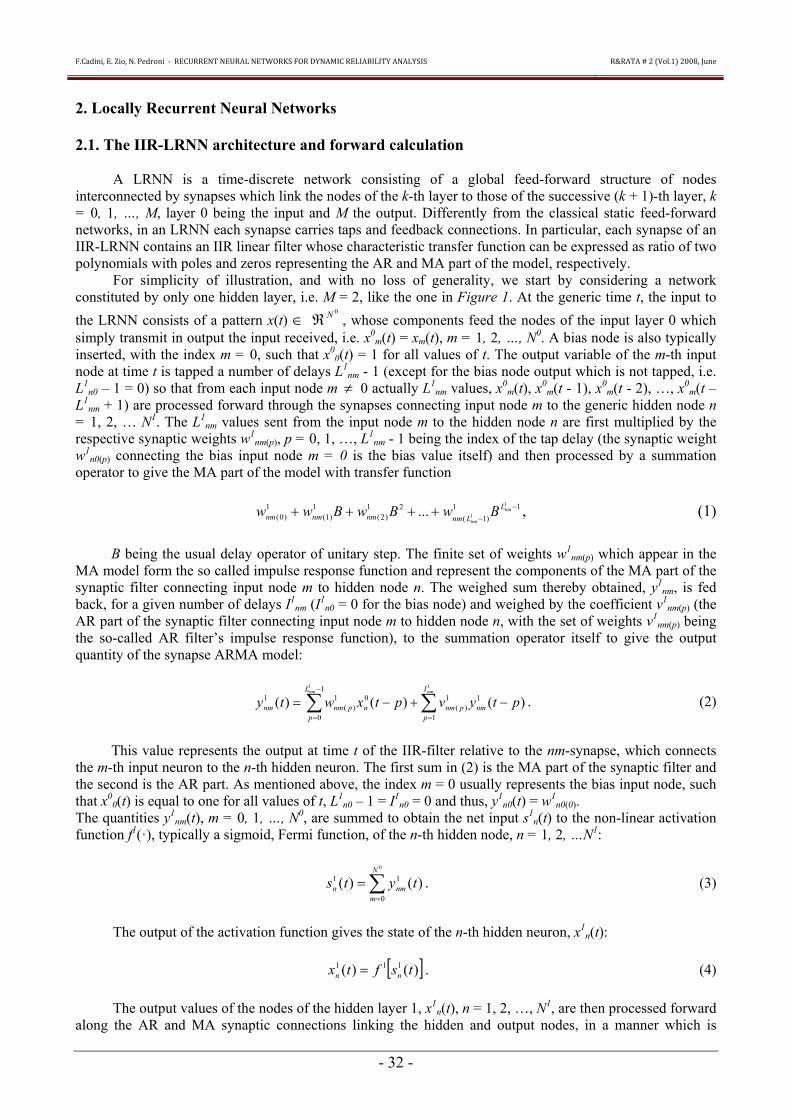
A LRNN is a time-discrete network consisting of a global feed-forward structure of nodes interconnected by synapses which link the nodes of the k-th layer to those of the successive (k + 1)-th layer k = 0 1 hellip M layer 0 being the input and M the output Differently from the classical static feed-forward networks in an LRNN each synapse carries taps and feedback connections In particular each synapse of an IIR-LRNN contains an IIR linear filter whose characteristic transfer function can be expressed as ratio of two polynomials with poles and zeros representing the AR and MA part of the model respectively
For simplicity of illustration and with no loss of generality we start by considering a network constituted by only one hidden layer ie M = 2 like the one in Figure 1 At the generic time t the input to the LRNN consists of a pattern x(t) isin
0Nreal whose components feed the nodes of the input layer 0 which simply transmit in output the input received ie x0
m(t) = xm(t) m = 1 2 hellip N0 A bias node is also typically inserted with the index m = 0 such that x0
0(t) = 1 for all values of t The output variable of the m-th input node at time t is tapped a number of delays L1
nm - 1 (except for the bias node output which is not tapped ie L1
n0 ndash 1 = 0) so that from each input node m ne 0 actually L1nm values x0
m(t) x0m(t - 1) x0
m(t - 2) hellip x0m(t ndash
L1nm + 1) are processed forward through the synapses connecting input node m to the generic hidden node n
= 1 2 hellip N1 The L1nm values sent from the input node m to the hidden node n are first multiplied by the
respective synaptic weights w1nm(p) p = 0 1 hellip L1
nm - 1 being the index of the tap delay (the synaptic weight w1
n0(p) connecting the bias input node m = 0 is the bias value itself) and then processed by a summation operator to give the MA part of the model with transfer function
11)1(
21)2(
1)1(
1)0(
1
1 minusminus
++++ nm
nm
LLnmnmnmnm BwBwBww (1)
B being the usual delay operator of unitary step The finite set of weights w1
nm(p) which appear in the MA model form the so called impulse response function and represent the components of the MA part of the synaptic filter connecting input node m to hidden node n The weighed sum thereby obtained y1
nm is fed back for a given number of delays I1
nm (I1n0 = 0 for the bias node) and weighed by the coefficient v1
nm(p) (the AR part of the synaptic filter connecting input node m to hidden node n with the set of weights v1
nm(p) being the so-called AR filterrsquos impulse response function) to the summation operator itself to give the output quantity of the synapse ARMA model
sumsum=
minus
=
minus+minus=11
1
11)(
1
0
01)(
1 )()()(nmnm I
pnmpnm
L
pnpnmnm ptyvptxwty (2)
This value represents the output at time t of the IIR-filter relative to the nm-synapse which connects
the m-th input neuron to the n-th hidden neuron The first sum in (2) is the MA part of the synaptic filter and the second is the AR part As mentioned above the index m = 0 usually represents the bias input node such that x0
0(t) is equal to one for all values of t L1n0 ndash 1 = I1
n0 = 0 and thus y1n0(t) = w1
n0(0) The quantities y1
nm(t) m = 0 1 hellip N0 are summed to obtain the net input s1n(t) to the non-linear activation
function f1(middot) typically a sigmoid Fermi function of the n-th hidden node n = 1 2 hellipN1
sum=
=0
0
11 )()(N
mnmn tyts (3)
The output of the activation function gives the state of the n-th hidden neuron x1
n(t)
[ ])()( 111 tsftx nn = (4)
The output values of the nodes of the hidden layer 1 x1n(t) n = 1 2 hellip N1 are then processed forward
along the AR and MA synaptic connections linking the hidden and output nodes in a manner which is
FCadini E Zio N Pedroni ‐ RECURRENT NEURAL NETWORKS FOR DYNAMIC RELIABILITY ANALYSIS
RampRATA 2 (Vol1) 2008 June
- 33 -
absolutely analogous to the processing between the input and hidden layers A bias node with index n = 0 is also typically inserted in the hidden layer such that x1
0(t) = 1 for all values of t The output variable of the n-th hidden node at time t is tapped a number of delays LM
rn ndash 1 ( = 0 for the bias node n = 0) so that from each hidden node n actually LM
rn values x1n(t) x1
n(t ndash 1) x1n(t ndash 2) hellip x1
n(t - LM
rn + 1) are processed forward through the MA-synapses connecting the hidden node n to the output node r = 1 2 hellip NM The LM
rn values sent from the hidden node n to the output node r are first multiplied by the respective synaptic weights wM
rn(p) p = 0 1 hellip LMrn ndash 1 being the index of the tap delay (the synaptic weight
wMr0 connecting the bias hidden node n = 0 is the bias value itself) and then processed by a summation
operator to give the MA part of the model with transfer function
1)1(
2)2()1()0( minus
minus++++
Mrn
Mrn
LMLrn
Mrn
Mrn
Mrn BwBwBww (5)
The sum of these values yM
rn is fed back for a given number of delays IMrn (IM
r0 = 0 for the bias node) and weighed by the coefficient vM
rn(p) (the AR part of the synaptic filter connecting hidden node n to output node r with the set of weights vM
rn(p) being the corresponding impulse response function) to the summation operator itself to give the output quantity of the synapse ARMA model
sumsum=
minus
=
minus+minus=Mrn
Mrn I
p
Mrn
Mprn
L
pn
Mprn
Mrn ptyvptxwty
1)(
1
0
1)( )()()( (6)
As mentioned before the index n = 0 represents the bias hidden node such that x1
0(t) is equal to one for all values of t LM
r0 ndash 1 = IMr0 = 0 and thus yM
r0(t) = wMr0(0)
The quantities yMrn(t) n = 0 1 hellip N1 are summed to obtain the net input sM
r(t) to the non-linear activation function fM(middot) also typically a sigmoid Fermi function of the r-th output node r = 1 2 hellip NM
sum=
=1
0
)()(N
n
Mrn
Mr tyts (7)
The output of the activation function gives the state of the r-th output neuron xM
r(t)
[ ])()( tsftx Mr
MMr = (8)
The extension of the above calculations to the case of multiple hidden layers (M gt 2) is
straightforward The time evolution of the generic neuron j belonging to the generic layer k = 1 2 hellip M is described by the following equations
[ ] )01()()( === jnodebiasthefortsftx kj
kkj (9)
summinus
=
=1
0
)()(kN
l
kjl
kj tyts (10)
sumsum=
minus
=
minus minus+minus=kjl
kjl I
p
kjl
kpjl
L
p
kl
kpjl
kjl ptyvptxwty
1)(
1
0
1)( )()()( (11)
Note that if all the synapses contain only the MA part (ie Ik
jl = 0 for all j k l) the architecture reduces to a FIR-MLP and if all the synaptic filters contain no memory (ie Lk
jl ndash 1 = 0 and Ikjl = 0 for all j
k l) the classical multilayered feed-forward static neural network is obtained 22 The Recursive Back-Propagation (RBP) algorithm for batch training
FCadini E Zio N Pedroni ‐ RECURRENT NEURAL NETWORKS FOR DYNAMIC RELIABILITY ANALYSIS
RampRATA 2 (Vol1) 2008 June
- 34 -
The Recursive Back-Propagation (RBP) training algorithm [6] is a gradient - based minimization
algorithm which makes use of a particular chain rule expansion rule expansion for the computation of the necessary derivatives A thorough description of the RBP training algorithm is given in the Appendix at the end of the paper
INPUT(k = 0)
HIDDEN (k = 1)
OUTPUT (k = 2 = M)
N0 = 1 N1 = 2 NM = 1 L1
11 ndash 1 = 1 LM11 - 1 = 2
L121 ndash 1 = 1 LM
12 ndash 1 = 1 I1
11 = 2 IM11 = 1
I121 = 1 IM
12 = 0
Figure 1 Scheme of an IIR-LRNN with one hidden layer 3 Simulating reactor neutron flux dynamics by LRNN
In general the training of an ANN to simulate the behaviour of a dynamic system can be quite a difficult task mainly due to the fact that the values of the system output vector y(t) at time t depend on both the forcing functions vector x() and the output y(middot) itself at previous steps
))1()1()(()( Θyxxy minusminus= tttFt (12)
where Θ is a set of adjustable parameters and F(middot) the non-linear mapping function describing the system dynamics
In this Section a locally recurrent neural network is trained to simulate the dynamic evolution of the neutron flux in a nuclear reactor 31 Problem formulation
The reference dynamics is described by a simple model based on a one group point kinetics equation with non-linear power reactivity feedback combined with Xenon and Iodine balance equations [8]
FCadini E Zio N Pedroni ‐ RECURRENT NEURAL NETWORKS FOR DYNAMIC RELIABILITY ANALYSIS
RampRATA 2 (Vol1) 2008 June
- 35 -
( )
IdtdI
XeXeIdt
dXe
Xecdt
d
IfI
XeXeIfXe
f
Xe
λγ
σλλγ
γσ
ρρ
minusΦΣ=
Φminusminus+ΦΣ=
Φ⎥⎥⎦
⎤
⎢⎢⎣
⎡Φminus
ΣminusΔ+=
ΦΛ 0
(13)
where Ф Xe and I are the values of flux Xenon and Iodine concentrations respectively
The reactor evolution is assumed to start from an equilibrium state at a nominal flux level Φ0= 466middot1012 ncm2s The initial reactivity needed to keep the steady state is ρ0 = 0071 and the Xenon and Iodine concentrations are Xe0 = 573middot1015 nucleicm3 and I0 = 581middot1015 nucleicm3 respectively In the following the values of flux Xenon and Iodine concentrations are normalized with respect to these steady state values
The objective is to design and train a LRNN to reproduce the neutron flux dynamics described by the system of differential equations (13) ie to estimate the evolution of the normalized neutron flux Φ(t) knowing the forcing function ρ(t)
Notice that the estimation is based only on the current values of reactivity These are fed in input to the locally recurrent model at each time step t thanks to the MA and AR parts of the synaptic filters an estimate of the neutron flux Φ(t) at time t is produced which recurrently accounts for past values of both the networkrsquos inputs and the estimated outputs viz
))1(ˆ)1()(()(ˆ ΘminusΦminus=Φ tttFt ρρ (14) where Ө is the set of adjustable parameters of the network model ie the synaptic weights
On the contrary the other non-measurable system state variables Xe(t) and I(t) are not fed in input to the LRNN the associated information remains distributed in the hidden layers and connections This renders the LRNN modelling task quite difficult 32 Design and training of the LRNN
The LRNN used in this work is characterized by three layers the input with two nodes (bias included) the hidden with six nodes (bias included) the output with one node A sigmoid activation function has been adopted for the hidden and output nodes
The training set has been constructed with Nt = 250 transients each one lasting T = 2000 minutes and sampled with a time step Δt of 40 minutes thus generating np = 50 patterns Notice that a temporal length of 2000 minutes allows the development of the long-term dynamics which are affected by the long-term Xe oscillations All data have been normalized in the range [02 08]
Each transient has been created varying the reactivity from its steady state value according to the following step function
⎩⎨⎧
Δ+=
ρρρ
ρ0
0)(t s
s
TtTt
gtle
(15)
where Ts is a random steady-state time interval and Δρ is random reactivity variation amplitude In order to build the 250 different transients for the training these two parameters have been randomly chosen within the ranges [0 2000] minutes and [-5middot10-4 +5middot10-4] respectively
The training procedure has been carried out on the available data for nepoch = 200 learning epochs (iterations) During each epoch every transient is repeatedly presented to the LRNN for nrep = 10 consecutive
FCadini E Zio N Pedroni ‐ RECURRENT NEURAL NETWORKS FOR DYNAMIC RELIABILITY ANALYSIS
RampRATA 2 (Vol1) 2008 June
- 36 -
times The weight updates are performed in batch at the end of each training sequence of length T No momentum term nor an adaptive learning rate [6] turned out necessary for increasing the efficiency of the training in this case
Ten training runs have been carried out to set the number of delays (orders of the MA and AR parts of the synaptic filters) so as to obtain a satisfactory performance of the LRNN measured in terms of a small root mean square error (RMSE) on the training set
As a result of these training runs the MA and AR orders of the IIR synaptic filters have been set to 12 and 10 respectively for both the hidden and the output neurons
33 Results
The trained LRNN is first verified with respect to its capability of reproducing the transients employed for the training itself This capability is a minimum requirement which however does not guarantee the proper general functioning of the LRNN when new transients different from those of training are fed into the network The evolution of the flux normalized with respect to the steady state value Φ0 corresponding to one sample training transients is shown in Figure 2 as expected the LRNN estimate of the output (crosses) is in satisfactory agreement with the actual transient (circles)
Notice the ability of the LRNN of dealing with both the short-term dynamics governed by the instantaneous variations of the forcing function (ie the reactivity step) and the long-term dynamics governed by Xe oscillations
0 400 800 1200 1600 200008
085
09
095
1
105
11
115
12
125
13
Time (min)
Nor
mal
ized
flux
Training transient step forcing function
truthLRNN
Figure 2 Comparison of the model-simulated normalized flux (circles) with the LRNN-estimated one (crosses) for two sample transients of the training set
331 Validation phase training like dynamics
The procedure for validating the generalization capability of the LRNN to transients different from those of training is based on Nt = 80 transients of T = 2000 minutes each initiated again by step variations in the forcing function ρ(t) as in eq (15) with timing and amplitude randomly sampled in the same ranges as in the training phase
The results reported in Figure 3 confirm the success of the training since the LRNN estimation errors are still small for these new transients Furthermore the computing time is about 5000 times lower than that required by the numerical solution of the model This makes the LRNN model very attractive for real time applications eg for control or diagnostic purposes and for applications for which repeated evaluations are required eg for uncertainty and sensitivity analyses
FCadini E Zio N Pedroni ‐ RECURRENT NEURAL NETWORKS FOR DYNAMIC RELIABILITY ANALYSIS
RampRATA 2 (Vol1) 2008 June
- 37 -
332 Test phase
The generalization capabilities of the trained and validated LRNN have been then tested on a new set of transients generated by forcing functions variations quite different from those used in both the training and the validation phases The test set consists of three
transients batches created by three functional shapes of the forcing function ρ(t) never seen by the LRNN
0 400 800 1200 1600 200006
07
08
09
1
11
12
13
Time (min)
Nor
mal
ized
flux
Validation transient step forcing function
truthLRNN
Figure 3 Comparison of the model-simulated normalized flux (circles) with the LRNN-estimated one (crosses) for one sample transient of the validation set
A ramp function
⎪⎩
⎪⎨
⎧
+gtΔ++leltΔminusΔ+
le=
=
vs
vsssvv
s
TTtTTtTTTtT
Ttt
)16()()(
)(
0
0
0
ρρρρρ
ρρ
where the steady-state time interval Ts (0 le Ts le 2000 min) the ramp variation time interval Tv (0 le Tv le 2000 min) and the reactivity variation amplitude Δρ (-5middot10-4 le Δρ le +510-4) are randomly extracted in their ranges of variation in order to generate the different transients
A sine function
)2sin()( ftt πρρ sdotΔ= (17)
where f is the oscillation frequency (1 le f le 2 min-1) and Δρ (-5middot10-4 le Δρ le +510-4) is the reactivity variation amplitude
Random reactivity variation amplitude with a uniform probability density function between -5middot10-4 and +5middot10-4
A total of Nt = 80 temporal sequences has been simulated for each batch producing a total of 240 test
transients The temporal length and the sampling time steps of each transient are the same as those of the training and validation sets (2000 and 40 minutes respectively)
Figures 4 5 and Figure 6 show a satisfactory agreement of the LRNN estimation with the model simulation even for cases quite different from the dynamic evolution considered during training
FCadini E Zio N Pedroni ‐ RECURRENT NEURAL NETWORKS FOR DYNAMIC RELIABILITY ANALYSIS
RampRATA 2 (Vol1) 2008 June
- 38 -
0 400 800 1200 1600 2000085
09
095
1
105
11
115
12
125
Time (min)
Nor
mal
ized
flux
Test transient ramp forcing function
truthLRNN
Figure 4 Comparison of the model-simulated normalized flux (circles) with the LRNN-estimated one (crosses) for one sample ramp transient of the test set
0 400 800 1200 1600 2000094
096
098
1
102
104
106
108
Time (min)
Nor
mal
ized
flux
Test transient sine forcing function
truthLRNN
Figure 5 Comparison of the model-simulated normalized flux (circles) with the LRNN-estimated one (crosses) for one sample sinusoidal transient of the test set
0 400 800 1200 1600 200007
08
09
1
11
12
13
14
Time (min)
Nor
mal
ized
flux
Test transient random forcing function
truthLRNN
Figure 6 Comparison of the model-simulated normalized flux (circles) with the LRNN-estimated one (crosses) for one sample random transient of the test set
These results are synthesized in Table 1 in terms of the following performance indices root mean
square error (RMSE) and mean absolute error (MAE)
FCadini E Zio N Pedroni ‐ RECURRENT NEURAL NETWORKS FOR DYNAMIC RELIABILITY ANALYSIS
RampRATA 2 (Vol1) 2008 June
- 39 -
Table 1 Values of the performance indices (RMSE and MAE) calculated over the training validation and test sets for the LRNN applied to the reactor neutron flux estimation
ERRORS
Set Forcing function
n of sequences RMSE MAE
Training Step 250 00037 00028 Validation Step 80 00098 00060
Test Ramp 80 00049 00039 Sine 80 00058 00051
Random 80 00063 00054
4 Conclusion
Dynamic reliability analyses entail the rapid simulation of the system dynamics under the different scenarios and configurations which occur during the system stochastic life evolution However the complexity and nonlinearities of the involved processes are such that analytical modelling becomes burdensome if at all feasible
In this paper the framework of Locally Recurrent Neural Networks (LRNNs) for non-linear dynamic simulation has been presented in detail The powerful dynamic modelling capabilities of this type of neural networks has been demonstrated on a case study concerning the evolution of the neutron flux in a nuclear reactor as described by a simple model of literature based on a one group point kinetics equation with non-linear power reactivity feedback coupled with the Xenon and Iodine balance equations
An Infinite Impulse Response-Locally Recurrent Neural Network (IIR-LRNN) has been successfully designed and trained with a Recursive Back-Propagation (RBP) algorithm to the difficult task of estimating the evolution of the neutron flux only knowing the reactivity evolution since the other non measurable system state variables ie Xenon and Iodine concentrations remain hidden
The findings of the research seem encouraging and confirmatory of the feasibility of using recurrent neural network models for the rapid and reliable system simulations needed in dynamic reliability analysis
References
[1] Aldemir T Siu N Mosleh A Cacciabue PC amp Goktepe BG (1994) Eds Reliability and Safety Assessment of Dynamic Process System NATO-ASI Series F Vol 120 Springer-Verlag Berlin
[2] Aldemir T Torri G Marseguerra M Zio E amp Borkowski J A (2003) Using point reactor models and genetic algorithms for on-line global xenon estimation in nuclear reactors Nuclear Technology 143 No 3 247-255
[3] Back A D amp Tsoi A C (1993) A simplified gradient algorithm for IIR synapse multi-layer perceptron Neural Comput 5 456-462
[4] Back A D et al (1994) A Unifying View of Some Training Algorithms for Multilayer Perceptrons with FIR Filter Synapses Proc IEEE Workshop Neural Netw Signal Process 146
[5] Boroushaki M et al (2003) Identification and control of a nuclear reactor core (VVER) using recurrent neural networks and fuzzy system IEEE Trans Nucl Sci 50(1) 159-174
[6] Campolucci P et al (1999) On-Line Learning Algorithms of Locally Recurrent Neural Networks IEEE Trans Neural Networks 10 253-271
[7] Carlos S Ginestar D Martorell S amp Serradell V (2003) Parameter estimation in thermalhydraulic models using the multidirectional search method Annals of Nuclear Energy 30 133-158
[8] Chernick J (1960) The dynamics of a xenon-controlled reactor Nuclear Science and Engineering 8 233-243
[9] Cojazzi G Izquierdo JM Melendez E amp Sanchez-Perea M (1992) The Reliability and Safety Assessment of Protection Systems by the Use of Dynamic Event Trees (DET) The DYLAM-TRETA package Proc XVIII annaul meeting Spanish Nuclear Society
[10] Devooght J amp Smidts C (1992) Probabilistic Reactor Dynamics I The Theory of Continuous Event Trees Nucl Sci and Eng 111 3 pp 229-240
FCadini E Zio N Pedroni ‐ RECURRENT NEURAL NETWORKS FOR DYNAMIC RELIABILITY ANALYSIS
RampRATA 2 (Vol1) 2008 June
- 40 -
[11] Haykin S (1994) Neural networks a comprehensive foundation New York IEEE Press [12] Hochreiter S amp Schmidhuber J (1997) Long short-term memory Neural Computation 9(8) 1735-
1780 [13] Izquierdo JM Hortal J Sanchez-Perea M amp Melendez E (1994) Automatic Generation of dynamic
Event Trees A Tool for Integrated Safety Assessment (ISA) Reliability and Safety Assessment of Dynamic Process System NATO-ASI Series F Vol 120 Springer-Verlag Berlin
[14] Labeau P E amp Zio E (1998) The Cell-to-Boundary Method in the Frame of Memorization-Based Monte Carlo Algorithms A New Computational Improvement in Dynamic Reliability Mathematics and Computers in Simulation Vol 47 No 2-5 329-347
[15] Labeau PE (1996) Probabilistic Dynamics Estimation of Generalized Unreliability Trhough Efficient Monte Carlo Simulation Annals of Nuclear Energy Vol 23 No 17 1355-1369
[16] Marseguerra M amp Zio E (1996) Monte Carlo approach to PSA for dynamic process systems Reliab Eng amp System Safety vol 52 227-241
[17] Narendra K S amp Parthasarathy K (1990) Identification and control of dynamical systems using neural networks IEEE Trans Neural Networks 1 4-27
[18] Pearlmutter B (1995) Gradient Calculations for Dynamic Recurrent Neural networks a Survey IEEE Trans Neural Networks 6 1212
[19] Siegelmann H amp Sontag E (1995) On the Computational Power of Neural Nets J Computers and Syst Sci 50 (1) 132
[20] Siu N (1994) Risk Assessment for Dynamic Systems An Overview Reliab Eng amp System Safety vol 43 43-74
FCadini E Zio N Pedroni ‐ RECURRENT NEURAL NETWORKS FOR DYNAMIC RELIABILITY ANALYSIS
RampRATA 2 (Vol1) 2008 June
- 41 -
Appendix the Recursive Back-Propagation (RBP) Algorithm for batch training
Consider one training temporal sequence of length T and denote by dr(t) r = 1 2 hellip NM the desired output value of the training sequence at time t
The instantaneous squared error at time t e2(t) is defined as the sum over all NM output nodes of the squared deviations of the network outputs xM
r(t) from the corresponding desired value in the training temporal sequence dr(t)
[ ]sum=
=MN
rr tete
1
22 )()( (1rsquo)
where )()()( txtdte M
rrr minus= (2rsquo)
The training algorithm aims at minimizing the global squared error E2 over the whole training sequence of length T
sum=
=T
t
teE1
22 )( (3rsquo)
This is achieved by modifying iteratively the network weights wk
jl(p) vkjl(p) along the gradient descent
viz
2
2
)(
2
)(
)(
2
)(
kpjl
kpjl
kpjl
kpjl
vEv
wEw
partpart
minus=Δ
partpart
minus=Δ
μ
μ
(4rsquo)
where μ is the learning rate Introducing the usual backpropagating error and delta quantities with respect to the output xk
j(t) and input sk
j(t) of the generic node j of layer k
)(2
1)(2
txEte kj
kj part
partminus= (5rsquo)
[ ])()(
)(
)(
)(21
)(21)(
22
tsfte
ts
tx
txE
tsEt
kjk
kj
kj
kj
kj
kj
kj
=
part
part
partpart
minus=partpart
minus=δ
(6rsquo)
the chain rule for the modification (4rsquo) of the MA and AR synaptic weights wk
jl(p) vkjl(p) can be written as
)(
)(
)()(
2
)(1
1)(
2
)(
kpjl
kj
T
t
kj
T
t
kpjl
kj
kj
kpjl
wts
t
wts
tsE
w
part
part=
part
part
partpart
minus=Δ
sum
sum
=
=
μδ
μ
FCadini E Zio N Pedroni ‐ RECURRENT NEURAL NETWORKS FOR DYNAMIC RELIABILITY ANALYSIS
RampRATA 2 (Vol1) 2008 June
- 42 -
)(
)(
)()(2
)(1
1 )(
2
)(
kpjl
kj
T
t
kj
T
tk
pjl
kj
kj
kpjl
vts
t
vts
tsEv
part
part=
part
part
partpart
minus=Δ
sum
sum
=
=
μδ
μ
(7rsquo)
Note that the weights updates (7rsquo) are performed in batch at the end of the training sequence of length
T From (10)
)()(
)()(
)()()()(k
pjl
kjl
kpjl
kj
kpjl
kjl
kpjl
kj
v
ty
v
ts
w
ty
w
ts
part
part=
part
part
part
part=
part
part (8rsquo)
so that from the differentiation of (11) one obtains
)(
)()(
)(1)(
1
)(k
pjl
kj
kjlI
kjl
klk
pjl
kj
w
tsvptx
w
ts
part
minuspartsum+minus=
part
part
=
minus ττ
τ (9rsquo)
)(
)()(
)(1)(
)(k
pjl
kj
kjlI
kjl
kjlk
pjl
kj
v
tsvpty
v
ts
part
minuspartsum+minus=
part
part
=
ττ
τ (10rsquo)
To compute δk
j(t) from (6rsquo) we must be able to compute ekj(t) Applying the chain rule to (5rsquo) one has
sum sumpart
part
partpart
minus=+
= =
+
+
1
1 1
1
1
2
)(
)(
)(21)(
kN
q
T
kj
kq
kq
kj tx
s
sEte
τ
τ
τ Mk lt (11rsquo)
Under the hypothesis of synaptic filter temporal causality (according to which the state of a node at
time t influences the network evolution only at successive times and not at previous ones) the summation along the time trajectory can start from τ = t Exploiting the definitions (6rsquo) and (8rsquo) changing the variables as τ ndash p t and considering that for the output layer ie k = M the derivative partE2partxM
j(t) can be computed directly from (2rsquo) the back-propagation of the error through the layers can be derived
⎪⎪
⎩
⎪⎪
⎨
⎧
sum sum ltpart
+part+
=
=minus
=
+
=
++tT
p
kN
q kj
kqik
q
j
kj
Mktx
ptypt
Mkeqte
te
0
1
1
11
)(
)()(
)2()(
)(δ
(12rsquo)
where from (11)
⎩⎨⎧ minuslele
+
sumpart
minus+part=
part
+part
++
+
=
++
+
010
)(
)(
)(
)(
11)(
)1min(
1
11
)(
1
otherwiseLpw
tx
ptyv
tx
pty
kqj
kpqj
pkqjI
kj
kqjk
qjkj
kqj
ττ
τ
(13rsquo)

FCadini E Zio N Pedroni ‐ RECURRENT NEURAL NETWORKS FOR DYNAMIC RELIABILITY ANALYSIS
RampRATA 2 (Vol1) 2008 June
- 31 -
process evolution In these cases one may resort to either simplified reduced analytical models such as those based on lumped effective parameters [2] [7] [8] or empirical models In both cases the model parameters have to be estimated so as to best fit to the available plant data
In the field of empirical modelling considerable interest is devoted to Artificial Neural Networks (ANNs) because of their capability of modelling non-linear dynamics and of automatically calibrating their parameters from representative inputoutput data [16] Whereas feedforward neural networks can model static inputoutput mappings but do not have the capability of reproducing the behaviour of dynamic systems dynamic Recurrent Neural Networks (RNNs) are recently attracting significant attention because of their potentials in temporal processing Indeed recurrent neural networks have been proven to constitute universal approximates of non-linear dynamic systems [19]
Two main methods exist for providing a neural network with dynamic behaviour the insertion of a buffer somewhere in the network to provide an explicit memory of the past inputs or the implementation of feedbacks
As for the first method it builds on the structure of feedforward networks where all input signals flow in one direction from input to output Then because a feedforward network does not have a dynamic memory tapped-delay-lines (temporal buffers) of the inputs are used The buffer can be applied at the network inputs only keeping the network internally static as in the buffered multilayer perceptron (MLP) [11] or at the input of each neuron as in the MLP with Finite Impulse Response (FIR) filter synapses (FIR-MLP) [4] The main disadvantage of the buffer approach is the limited past-history horizon which needs to be used in order to keep the size of the network computationally manageable thereby preventing modelling of arbitrary long time dependencies between inputs and outputs [12] It is also difficult to set the length of the buffer given a certain application
Regarding the second method the most general example of implementation of feedbacks in a neural network is the fully recurrent neural network constituted by a single layer of neurons fully interconnected with each other or by several such layers [18] Because of the required large structural complexity of this network in recent years growing efforts have been propounded in developing methods for implementing temporal dynamic feedback connections into the widely used multi-layered feedforward neural networks Recurrent connections can be added by using two main types of recurrence or feedback external or internal External recurrence is obtained for example by feeding back the outputs to the input of the network as in NARX networks [5] [17] internal recurrence is obtained by feeding back the outputs of neurons of a given layer in inputs to neurons of the same layer giving rise to the so called Locally Recurrent Neural Networks (LRNNs) [6]
The major advantages of LRNNs with respect to the buffered tapped-delayed feedforward networks and to the fully recurrent networks are [6] 1) the hierarchic multilayer topology which they are based on is well known and efficient 2) the use of dynamic neurons allows to limit the number of neurons required for modelling a given dynamic system contrary to the tapped-delayed networks 3) the training procedures for properly adjusting the network weights are significantly simpler and faster than those for the fully recurrent networks
In this paper an Infinite Impulse Response-Locally Recurrent Neural Network (IIR-LRNN) is adopted together with the Recursive Back-Propagation (RBP) algorithm for its batch training [6] In the IIR-LRNN the synapses are implemented as Infinite Impulse Response digital filters which provide the network with system state memory
The proposed neural approach is applied to a highly non-linear dynamic system of literature the continuous time Chernick model of a simplified nuclear reactor [8] the IIR-LRNN is devised to estimate the neutron flux temporal evolution only knowing the reactivity forcing function The IIR-LRNN ability of dealing with both the short-term dynamics governed by the instantaneous variations of the reactivity and the long-term dynamics governed by Xe oscillations is verified by extensive simulations on training validation and test transients
The paper is organized as follows in Section 2 the IIR-LRNN architecture is presented in detail together with the RBP training algorithm in Section 3 the adopted neural approach is applied to simulate the reactor neutron flux dynamics Finally some conclusions are proposed in the last Section
FCadini E Zio N Pedroni ‐ RECURRENT NEURAL NETWORKS FOR DYNAMIC RELIABILITY ANALYSIS
RampRATA 2 (Vol1) 2008 June
- 32 -
2 Locally Recurrent Neural Networks 21 The IIR-LRNN architecture and forward calculation
A LRNN is a time-discrete network consisting of a global feed-forward structure of nodes interconnected by synapses which link the nodes of the k-th layer to those of the successive (k + 1)-th layer k = 0 1 hellip M layer 0 being the input and M the output Differently from the classical static feed-forward networks in an LRNN each synapse carries taps and feedback connections In particular each synapse of an IIR-LRNN contains an IIR linear filter whose characteristic transfer function can be expressed as ratio of two polynomials with poles and zeros representing the AR and MA part of the model respectively
For simplicity of illustration and with no loss of generality we start by considering a network constituted by only one hidden layer ie M = 2 like the one in Figure 1 At the generic time t the input to the LRNN consists of a pattern x(t) isin
0Nreal whose components feed the nodes of the input layer 0 which simply transmit in output the input received ie x0
m(t) = xm(t) m = 1 2 hellip N0 A bias node is also typically inserted with the index m = 0 such that x0
0(t) = 1 for all values of t The output variable of the m-th input node at time t is tapped a number of delays L1
nm - 1 (except for the bias node output which is not tapped ie L1
n0 ndash 1 = 0) so that from each input node m ne 0 actually L1nm values x0
m(t) x0m(t - 1) x0
m(t - 2) hellip x0m(t ndash
L1nm + 1) are processed forward through the synapses connecting input node m to the generic hidden node n
= 1 2 hellip N1 The L1nm values sent from the input node m to the hidden node n are first multiplied by the
respective synaptic weights w1nm(p) p = 0 1 hellip L1
nm - 1 being the index of the tap delay (the synaptic weight w1
n0(p) connecting the bias input node m = 0 is the bias value itself) and then processed by a summation operator to give the MA part of the model with transfer function
11)1(
21)2(
1)1(
1)0(
1
1 minusminus
++++ nm
nm
LLnmnmnmnm BwBwBww (1)
B being the usual delay operator of unitary step The finite set of weights w1
nm(p) which appear in the MA model form the so called impulse response function and represent the components of the MA part of the synaptic filter connecting input node m to hidden node n The weighed sum thereby obtained y1
nm is fed back for a given number of delays I1
nm (I1n0 = 0 for the bias node) and weighed by the coefficient v1
nm(p) (the AR part of the synaptic filter connecting input node m to hidden node n with the set of weights v1
nm(p) being the so-called AR filterrsquos impulse response function) to the summation operator itself to give the output quantity of the synapse ARMA model
sumsum=
minus
=
minus+minus=11
1
11)(
1
0
01)(
1 )()()(nmnm I
pnmpnm
L
pnpnmnm ptyvptxwty (2)
This value represents the output at time t of the IIR-filter relative to the nm-synapse which connects
the m-th input neuron to the n-th hidden neuron The first sum in (2) is the MA part of the synaptic filter and the second is the AR part As mentioned above the index m = 0 usually represents the bias input node such that x0
0(t) is equal to one for all values of t L1n0 ndash 1 = I1
n0 = 0 and thus y1n0(t) = w1
n0(0) The quantities y1
nm(t) m = 0 1 hellip N0 are summed to obtain the net input s1n(t) to the non-linear activation
function f1(middot) typically a sigmoid Fermi function of the n-th hidden node n = 1 2 hellipN1
sum=
=0
0
11 )()(N
mnmn tyts (3)
The output of the activation function gives the state of the n-th hidden neuron x1
n(t)
[ ])()( 111 tsftx nn = (4)
The output values of the nodes of the hidden layer 1 x1n(t) n = 1 2 hellip N1 are then processed forward
along the AR and MA synaptic connections linking the hidden and output nodes in a manner which is
FCadini E Zio N Pedroni ‐ RECURRENT NEURAL NETWORKS FOR DYNAMIC RELIABILITY ANALYSIS
RampRATA 2 (Vol1) 2008 June
- 33 -
absolutely analogous to the processing between the input and hidden layers A bias node with index n = 0 is also typically inserted in the hidden layer such that x1
0(t) = 1 for all values of t The output variable of the n-th hidden node at time t is tapped a number of delays LM
rn ndash 1 ( = 0 for the bias node n = 0) so that from each hidden node n actually LM
rn values x1n(t) x1
n(t ndash 1) x1n(t ndash 2) hellip x1
n(t - LM
rn + 1) are processed forward through the MA-synapses connecting the hidden node n to the output node r = 1 2 hellip NM The LM
rn values sent from the hidden node n to the output node r are first multiplied by the respective synaptic weights wM
rn(p) p = 0 1 hellip LMrn ndash 1 being the index of the tap delay (the synaptic weight
wMr0 connecting the bias hidden node n = 0 is the bias value itself) and then processed by a summation
operator to give the MA part of the model with transfer function
1)1(
2)2()1()0( minus
minus++++
Mrn
Mrn
LMLrn
Mrn
Mrn
Mrn BwBwBww (5)
The sum of these values yM
rn is fed back for a given number of delays IMrn (IM
r0 = 0 for the bias node) and weighed by the coefficient vM
rn(p) (the AR part of the synaptic filter connecting hidden node n to output node r with the set of weights vM
rn(p) being the corresponding impulse response function) to the summation operator itself to give the output quantity of the synapse ARMA model
sumsum=
minus
=
minus+minus=Mrn
Mrn I
p
Mrn
Mprn
L
pn
Mprn
Mrn ptyvptxwty
1)(
1
0
1)( )()()( (6)
As mentioned before the index n = 0 represents the bias hidden node such that x1
0(t) is equal to one for all values of t LM
r0 ndash 1 = IMr0 = 0 and thus yM
r0(t) = wMr0(0)
The quantities yMrn(t) n = 0 1 hellip N1 are summed to obtain the net input sM
r(t) to the non-linear activation function fM(middot) also typically a sigmoid Fermi function of the r-th output node r = 1 2 hellip NM
sum=
=1
0
)()(N
n
Mrn
Mr tyts (7)
The output of the activation function gives the state of the r-th output neuron xM
r(t)
[ ])()( tsftx Mr
MMr = (8)
The extension of the above calculations to the case of multiple hidden layers (M gt 2) is
straightforward The time evolution of the generic neuron j belonging to the generic layer k = 1 2 hellip M is described by the following equations
[ ] )01()()( === jnodebiasthefortsftx kj
kkj (9)
summinus
=
=1
0
)()(kN
l
kjl
kj tyts (10)
sumsum=
minus
=
minus minus+minus=kjl
kjl I
p
kjl
kpjl
L
p
kl
kpjl
kjl ptyvptxwty
1)(
1
0
1)( )()()( (11)
Note that if all the synapses contain only the MA part (ie Ik
jl = 0 for all j k l) the architecture reduces to a FIR-MLP and if all the synaptic filters contain no memory (ie Lk
jl ndash 1 = 0 and Ikjl = 0 for all j
k l) the classical multilayered feed-forward static neural network is obtained 22 The Recursive Back-Propagation (RBP) algorithm for batch training
FCadini E Zio N Pedroni ‐ RECURRENT NEURAL NETWORKS FOR DYNAMIC RELIABILITY ANALYSIS
RampRATA 2 (Vol1) 2008 June
- 34 -
The Recursive Back-Propagation (RBP) training algorithm [6] is a gradient - based minimization
algorithm which makes use of a particular chain rule expansion rule expansion for the computation of the necessary derivatives A thorough description of the RBP training algorithm is given in the Appendix at the end of the paper
INPUT(k = 0)
HIDDEN (k = 1)
OUTPUT (k = 2 = M)
N0 = 1 N1 = 2 NM = 1 L1
11 ndash 1 = 1 LM11 - 1 = 2
L121 ndash 1 = 1 LM
12 ndash 1 = 1 I1
11 = 2 IM11 = 1
I121 = 1 IM
12 = 0
Figure 1 Scheme of an IIR-LRNN with one hidden layer 3 Simulating reactor neutron flux dynamics by LRNN
In general the training of an ANN to simulate the behaviour of a dynamic system can be quite a difficult task mainly due to the fact that the values of the system output vector y(t) at time t depend on both the forcing functions vector x() and the output y(middot) itself at previous steps
))1()1()(()( Θyxxy minusminus= tttFt (12)
where Θ is a set of adjustable parameters and F(middot) the non-linear mapping function describing the system dynamics
In this Section a locally recurrent neural network is trained to simulate the dynamic evolution of the neutron flux in a nuclear reactor 31 Problem formulation
The reference dynamics is described by a simple model based on a one group point kinetics equation with non-linear power reactivity feedback combined with Xenon and Iodine balance equations [8]
FCadini E Zio N Pedroni ‐ RECURRENT NEURAL NETWORKS FOR DYNAMIC RELIABILITY ANALYSIS
RampRATA 2 (Vol1) 2008 June
- 35 -
( )
IdtdI
XeXeIdt
dXe
Xecdt
d
IfI
XeXeIfXe
f
Xe
λγ
σλλγ
γσ
ρρ
minusΦΣ=
Φminusminus+ΦΣ=
Φ⎥⎥⎦
⎤
⎢⎢⎣
⎡Φminus
ΣminusΔ+=
ΦΛ 0
(13)
where Ф Xe and I are the values of flux Xenon and Iodine concentrations respectively
The reactor evolution is assumed to start from an equilibrium state at a nominal flux level Φ0= 466middot1012 ncm2s The initial reactivity needed to keep the steady state is ρ0 = 0071 and the Xenon and Iodine concentrations are Xe0 = 573middot1015 nucleicm3 and I0 = 581middot1015 nucleicm3 respectively In the following the values of flux Xenon and Iodine concentrations are normalized with respect to these steady state values
The objective is to design and train a LRNN to reproduce the neutron flux dynamics described by the system of differential equations (13) ie to estimate the evolution of the normalized neutron flux Φ(t) knowing the forcing function ρ(t)
Notice that the estimation is based only on the current values of reactivity These are fed in input to the locally recurrent model at each time step t thanks to the MA and AR parts of the synaptic filters an estimate of the neutron flux Φ(t) at time t is produced which recurrently accounts for past values of both the networkrsquos inputs and the estimated outputs viz
))1(ˆ)1()(()(ˆ ΘminusΦminus=Φ tttFt ρρ (14) where Ө is the set of adjustable parameters of the network model ie the synaptic weights
On the contrary the other non-measurable system state variables Xe(t) and I(t) are not fed in input to the LRNN the associated information remains distributed in the hidden layers and connections This renders the LRNN modelling task quite difficult 32 Design and training of the LRNN
The LRNN used in this work is characterized by three layers the input with two nodes (bias included) the hidden with six nodes (bias included) the output with one node A sigmoid activation function has been adopted for the hidden and output nodes
The training set has been constructed with Nt = 250 transients each one lasting T = 2000 minutes and sampled with a time step Δt of 40 minutes thus generating np = 50 patterns Notice that a temporal length of 2000 minutes allows the development of the long-term dynamics which are affected by the long-term Xe oscillations All data have been normalized in the range [02 08]
Each transient has been created varying the reactivity from its steady state value according to the following step function
⎩⎨⎧
Δ+=
ρρρ
ρ0
0)(t s
s
TtTt
gtle
(15)
where Ts is a random steady-state time interval and Δρ is random reactivity variation amplitude In order to build the 250 different transients for the training these two parameters have been randomly chosen within the ranges [0 2000] minutes and [-5middot10-4 +5middot10-4] respectively
The training procedure has been carried out on the available data for nepoch = 200 learning epochs (iterations) During each epoch every transient is repeatedly presented to the LRNN for nrep = 10 consecutive
FCadini E Zio N Pedroni ‐ RECURRENT NEURAL NETWORKS FOR DYNAMIC RELIABILITY ANALYSIS
RampRATA 2 (Vol1) 2008 June
- 36 -
times The weight updates are performed in batch at the end of each training sequence of length T No momentum term nor an adaptive learning rate [6] turned out necessary for increasing the efficiency of the training in this case
Ten training runs have been carried out to set the number of delays (orders of the MA and AR parts of the synaptic filters) so as to obtain a satisfactory performance of the LRNN measured in terms of a small root mean square error (RMSE) on the training set
As a result of these training runs the MA and AR orders of the IIR synaptic filters have been set to 12 and 10 respectively for both the hidden and the output neurons
33 Results
The trained LRNN is first verified with respect to its capability of reproducing the transients employed for the training itself This capability is a minimum requirement which however does not guarantee the proper general functioning of the LRNN when new transients different from those of training are fed into the network The evolution of the flux normalized with respect to the steady state value Φ0 corresponding to one sample training transients is shown in Figure 2 as expected the LRNN estimate of the output (crosses) is in satisfactory agreement with the actual transient (circles)
Notice the ability of the LRNN of dealing with both the short-term dynamics governed by the instantaneous variations of the forcing function (ie the reactivity step) and the long-term dynamics governed by Xe oscillations
0 400 800 1200 1600 200008
085
09
095
1
105
11
115
12
125
13
Time (min)
Nor
mal
ized
flux
Training transient step forcing function
truthLRNN
Figure 2 Comparison of the model-simulated normalized flux (circles) with the LRNN-estimated one (crosses) for two sample transients of the training set
331 Validation phase training like dynamics
The procedure for validating the generalization capability of the LRNN to transients different from those of training is based on Nt = 80 transients of T = 2000 minutes each initiated again by step variations in the forcing function ρ(t) as in eq (15) with timing and amplitude randomly sampled in the same ranges as in the training phase
The results reported in Figure 3 confirm the success of the training since the LRNN estimation errors are still small for these new transients Furthermore the computing time is about 5000 times lower than that required by the numerical solution of the model This makes the LRNN model very attractive for real time applications eg for control or diagnostic purposes and for applications for which repeated evaluations are required eg for uncertainty and sensitivity analyses
FCadini E Zio N Pedroni ‐ RECURRENT NEURAL NETWORKS FOR DYNAMIC RELIABILITY ANALYSIS
RampRATA 2 (Vol1) 2008 June
- 37 -
332 Test phase
The generalization capabilities of the trained and validated LRNN have been then tested on a new set of transients generated by forcing functions variations quite different from those used in both the training and the validation phases The test set consists of three
transients batches created by three functional shapes of the forcing function ρ(t) never seen by the LRNN
0 400 800 1200 1600 200006
07
08
09
1
11
12
13
Time (min)
Nor
mal
ized
flux
Validation transient step forcing function
truthLRNN
Figure 3 Comparison of the model-simulated normalized flux (circles) with the LRNN-estimated one (crosses) for one sample transient of the validation set
A ramp function
⎪⎩
⎪⎨
⎧
+gtΔ++leltΔminusΔ+
le=
=
vs
vsssvv
s
TTtTTtTTTtT
Ttt
)16()()(
)(
0
0
0
ρρρρρ
ρρ
where the steady-state time interval Ts (0 le Ts le 2000 min) the ramp variation time interval Tv (0 le Tv le 2000 min) and the reactivity variation amplitude Δρ (-5middot10-4 le Δρ le +510-4) are randomly extracted in their ranges of variation in order to generate the different transients
A sine function
)2sin()( ftt πρρ sdotΔ= (17)
where f is the oscillation frequency (1 le f le 2 min-1) and Δρ (-5middot10-4 le Δρ le +510-4) is the reactivity variation amplitude
Random reactivity variation amplitude with a uniform probability density function between -5middot10-4 and +5middot10-4
A total of Nt = 80 temporal sequences has been simulated for each batch producing a total of 240 test
transients The temporal length and the sampling time steps of each transient are the same as those of the training and validation sets (2000 and 40 minutes respectively)
Figures 4 5 and Figure 6 show a satisfactory agreement of the LRNN estimation with the model simulation even for cases quite different from the dynamic evolution considered during training
FCadini E Zio N Pedroni ‐ RECURRENT NEURAL NETWORKS FOR DYNAMIC RELIABILITY ANALYSIS
RampRATA 2 (Vol1) 2008 June
- 38 -
0 400 800 1200 1600 2000085
09
095
1
105
11
115
12
125
Time (min)
Nor
mal
ized
flux
Test transient ramp forcing function
truthLRNN
Figure 4 Comparison of the model-simulated normalized flux (circles) with the LRNN-estimated one (crosses) for one sample ramp transient of the test set
0 400 800 1200 1600 2000094
096
098
1
102
104
106
108
Time (min)
Nor
mal
ized
flux
Test transient sine forcing function
truthLRNN
Figure 5 Comparison of the model-simulated normalized flux (circles) with the LRNN-estimated one (crosses) for one sample sinusoidal transient of the test set
0 400 800 1200 1600 200007
08
09
1
11
12
13
14
Time (min)
Nor
mal
ized
flux
Test transient random forcing function
truthLRNN
Figure 6 Comparison of the model-simulated normalized flux (circles) with the LRNN-estimated one (crosses) for one sample random transient of the test set
These results are synthesized in Table 1 in terms of the following performance indices root mean
square error (RMSE) and mean absolute error (MAE)
FCadini E Zio N Pedroni ‐ RECURRENT NEURAL NETWORKS FOR DYNAMIC RELIABILITY ANALYSIS
RampRATA 2 (Vol1) 2008 June
- 39 -
Table 1 Values of the performance indices (RMSE and MAE) calculated over the training validation and test sets for the LRNN applied to the reactor neutron flux estimation
ERRORS
Set Forcing function
n of sequences RMSE MAE
Training Step 250 00037 00028 Validation Step 80 00098 00060
Test Ramp 80 00049 00039 Sine 80 00058 00051
Random 80 00063 00054
4 Conclusion
Dynamic reliability analyses entail the rapid simulation of the system dynamics under the different scenarios and configurations which occur during the system stochastic life evolution However the complexity and nonlinearities of the involved processes are such that analytical modelling becomes burdensome if at all feasible
In this paper the framework of Locally Recurrent Neural Networks (LRNNs) for non-linear dynamic simulation has been presented in detail The powerful dynamic modelling capabilities of this type of neural networks has been demonstrated on a case study concerning the evolution of the neutron flux in a nuclear reactor as described by a simple model of literature based on a one group point kinetics equation with non-linear power reactivity feedback coupled with the Xenon and Iodine balance equations
An Infinite Impulse Response-Locally Recurrent Neural Network (IIR-LRNN) has been successfully designed and trained with a Recursive Back-Propagation (RBP) algorithm to the difficult task of estimating the evolution of the neutron flux only knowing the reactivity evolution since the other non measurable system state variables ie Xenon and Iodine concentrations remain hidden
The findings of the research seem encouraging and confirmatory of the feasibility of using recurrent neural network models for the rapid and reliable system simulations needed in dynamic reliability analysis
References
[1] Aldemir T Siu N Mosleh A Cacciabue PC amp Goktepe BG (1994) Eds Reliability and Safety Assessment of Dynamic Process System NATO-ASI Series F Vol 120 Springer-Verlag Berlin
[2] Aldemir T Torri G Marseguerra M Zio E amp Borkowski J A (2003) Using point reactor models and genetic algorithms for on-line global xenon estimation in nuclear reactors Nuclear Technology 143 No 3 247-255
[3] Back A D amp Tsoi A C (1993) A simplified gradient algorithm for IIR synapse multi-layer perceptron Neural Comput 5 456-462
[4] Back A D et al (1994) A Unifying View of Some Training Algorithms for Multilayer Perceptrons with FIR Filter Synapses Proc IEEE Workshop Neural Netw Signal Process 146
[5] Boroushaki M et al (2003) Identification and control of a nuclear reactor core (VVER) using recurrent neural networks and fuzzy system IEEE Trans Nucl Sci 50(1) 159-174
[6] Campolucci P et al (1999) On-Line Learning Algorithms of Locally Recurrent Neural Networks IEEE Trans Neural Networks 10 253-271
[7] Carlos S Ginestar D Martorell S amp Serradell V (2003) Parameter estimation in thermalhydraulic models using the multidirectional search method Annals of Nuclear Energy 30 133-158
[8] Chernick J (1960) The dynamics of a xenon-controlled reactor Nuclear Science and Engineering 8 233-243
[9] Cojazzi G Izquierdo JM Melendez E amp Sanchez-Perea M (1992) The Reliability and Safety Assessment of Protection Systems by the Use of Dynamic Event Trees (DET) The DYLAM-TRETA package Proc XVIII annaul meeting Spanish Nuclear Society
[10] Devooght J amp Smidts C (1992) Probabilistic Reactor Dynamics I The Theory of Continuous Event Trees Nucl Sci and Eng 111 3 pp 229-240
FCadini E Zio N Pedroni ‐ RECURRENT NEURAL NETWORKS FOR DYNAMIC RELIABILITY ANALYSIS
RampRATA 2 (Vol1) 2008 June
- 40 -
[11] Haykin S (1994) Neural networks a comprehensive foundation New York IEEE Press [12] Hochreiter S amp Schmidhuber J (1997) Long short-term memory Neural Computation 9(8) 1735-
1780 [13] Izquierdo JM Hortal J Sanchez-Perea M amp Melendez E (1994) Automatic Generation of dynamic
Event Trees A Tool for Integrated Safety Assessment (ISA) Reliability and Safety Assessment of Dynamic Process System NATO-ASI Series F Vol 120 Springer-Verlag Berlin
[14] Labeau P E amp Zio E (1998) The Cell-to-Boundary Method in the Frame of Memorization-Based Monte Carlo Algorithms A New Computational Improvement in Dynamic Reliability Mathematics and Computers in Simulation Vol 47 No 2-5 329-347
[15] Labeau PE (1996) Probabilistic Dynamics Estimation of Generalized Unreliability Trhough Efficient Monte Carlo Simulation Annals of Nuclear Energy Vol 23 No 17 1355-1369
[16] Marseguerra M amp Zio E (1996) Monte Carlo approach to PSA for dynamic process systems Reliab Eng amp System Safety vol 52 227-241
[17] Narendra K S amp Parthasarathy K (1990) Identification and control of dynamical systems using neural networks IEEE Trans Neural Networks 1 4-27
[18] Pearlmutter B (1995) Gradient Calculations for Dynamic Recurrent Neural networks a Survey IEEE Trans Neural Networks 6 1212
[19] Siegelmann H amp Sontag E (1995) On the Computational Power of Neural Nets J Computers and Syst Sci 50 (1) 132
[20] Siu N (1994) Risk Assessment for Dynamic Systems An Overview Reliab Eng amp System Safety vol 43 43-74
FCadini E Zio N Pedroni ‐ RECURRENT NEURAL NETWORKS FOR DYNAMIC RELIABILITY ANALYSIS
RampRATA 2 (Vol1) 2008 June
- 41 -
Appendix the Recursive Back-Propagation (RBP) Algorithm for batch training
Consider one training temporal sequence of length T and denote by dr(t) r = 1 2 hellip NM the desired output value of the training sequence at time t
The instantaneous squared error at time t e2(t) is defined as the sum over all NM output nodes of the squared deviations of the network outputs xM
r(t) from the corresponding desired value in the training temporal sequence dr(t)
[ ]sum=
=MN
rr tete
1
22 )()( (1rsquo)
where )()()( txtdte M
rrr minus= (2rsquo)
The training algorithm aims at minimizing the global squared error E2 over the whole training sequence of length T
sum=
=T
t
teE1
22 )( (3rsquo)
This is achieved by modifying iteratively the network weights wk
jl(p) vkjl(p) along the gradient descent
viz
2
2
)(
2
)(
)(
2
)(
kpjl
kpjl
kpjl
kpjl
vEv
wEw
partpart
minus=Δ
partpart
minus=Δ
μ
μ
(4rsquo)
where μ is the learning rate Introducing the usual backpropagating error and delta quantities with respect to the output xk
j(t) and input sk
j(t) of the generic node j of layer k
)(2
1)(2
txEte kj
kj part
partminus= (5rsquo)
[ ])()(
)(
)(
)(21
)(21)(
22
tsfte
ts
tx
txE
tsEt
kjk
kj
kj
kj
kj
kj
kj
=
part
part
partpart
minus=partpart
minus=δ
(6rsquo)
the chain rule for the modification (4rsquo) of the MA and AR synaptic weights wk
jl(p) vkjl(p) can be written as
)(
)(
)()(
2
)(1
1)(
2
)(
kpjl
kj
T
t
kj
T
t
kpjl
kj
kj
kpjl
wts
t
wts
tsE
w
part
part=
part
part
partpart
minus=Δ
sum
sum
=
=
μδ
μ
FCadini E Zio N Pedroni ‐ RECURRENT NEURAL NETWORKS FOR DYNAMIC RELIABILITY ANALYSIS
RampRATA 2 (Vol1) 2008 June
- 42 -
)(
)(
)()(2
)(1
1 )(
2
)(
kpjl
kj
T
t
kj
T
tk
pjl
kj
kj
kpjl
vts
t
vts
tsEv
part
part=
part
part
partpart
minus=Δ
sum
sum
=
=
μδ
μ
(7rsquo)
Note that the weights updates (7rsquo) are performed in batch at the end of the training sequence of length
T From (10)
)()(
)()(
)()()()(k
pjl
kjl
kpjl
kj
kpjl
kjl
kpjl
kj
v
ty
v
ts
w
ty
w
ts
part
part=
part
part
part
part=
part
part (8rsquo)
so that from the differentiation of (11) one obtains
)(
)()(
)(1)(
1
)(k
pjl
kj
kjlI
kjl
klk
pjl
kj
w
tsvptx
w
ts
part
minuspartsum+minus=
part
part
=
minus ττ
τ (9rsquo)
)(
)()(
)(1)(
)(k
pjl
kj
kjlI
kjl
kjlk
pjl
kj
v
tsvpty
v
ts
part
minuspartsum+minus=
part
part
=
ττ
τ (10rsquo)
To compute δk
j(t) from (6rsquo) we must be able to compute ekj(t) Applying the chain rule to (5rsquo) one has
sum sumpart
part
partpart
minus=+
= =
+
+
1
1 1
1
1
2
)(
)(
)(21)(
kN
q
T
kj
kq
kq
kj tx
s
sEte
τ
τ
τ Mk lt (11rsquo)
Under the hypothesis of synaptic filter temporal causality (according to which the state of a node at
time t influences the network evolution only at successive times and not at previous ones) the summation along the time trajectory can start from τ = t Exploiting the definitions (6rsquo) and (8rsquo) changing the variables as τ ndash p t and considering that for the output layer ie k = M the derivative partE2partxM
j(t) can be computed directly from (2rsquo) the back-propagation of the error through the layers can be derived
⎪⎪
⎩
⎪⎪
⎨
⎧
sum sum ltpart
+part+
=
=minus
=
+
=
++tT
p
kN
q kj
kqik
q
j
kj
Mktx
ptypt
Mkeqte
te
0
1
1
11
)(
)()(
)2()(
)(δ
(12rsquo)
where from (11)
⎩⎨⎧ minuslele
+
sumpart
minus+part=
part
+part
++
+
=
++
+
010
)(
)(
)(
)(
11)(
)1min(
1
11
)(
1
otherwiseLpw
tx
ptyv
tx
pty
kqj
kpqj
pkqjI
kj
kqjk
qjkj
kqj
ττ
τ
(13rsquo)
FCadini E Zio N Pedroni ‐ RECURRENT NEURAL NETWORKS FOR DYNAMIC RELIABILITY ANALYSIS
RampRATA 2 (Vol1) 2008 June
- 32 -
2 Locally Recurrent Neural Networks 21 The IIR-LRNN architecture and forward calculation
A LRNN is a time-discrete network consisting of a global feed-forward structure of nodes interconnected by synapses which link the nodes of the k-th layer to those of the successive (k + 1)-th layer k = 0 1 hellip M layer 0 being the input and M the output Differently from the classical static feed-forward networks in an LRNN each synapse carries taps and feedback connections In particular each synapse of an IIR-LRNN contains an IIR linear filter whose characteristic transfer function can be expressed as ratio of two polynomials with poles and zeros representing the AR and MA part of the model respectively
For simplicity of illustration and with no loss of generality we start by considering a network constituted by only one hidden layer ie M = 2 like the one in Figure 1 At the generic time t the input to the LRNN consists of a pattern x(t) isin
0Nreal whose components feed the nodes of the input layer 0 which simply transmit in output the input received ie x0
m(t) = xm(t) m = 1 2 hellip N0 A bias node is also typically inserted with the index m = 0 such that x0
0(t) = 1 for all values of t The output variable of the m-th input node at time t is tapped a number of delays L1
nm - 1 (except for the bias node output which is not tapped ie L1
n0 ndash 1 = 0) so that from each input node m ne 0 actually L1nm values x0
m(t) x0m(t - 1) x0
m(t - 2) hellip x0m(t ndash
L1nm + 1) are processed forward through the synapses connecting input node m to the generic hidden node n
= 1 2 hellip N1 The L1nm values sent from the input node m to the hidden node n are first multiplied by the
respective synaptic weights w1nm(p) p = 0 1 hellip L1
nm - 1 being the index of the tap delay (the synaptic weight w1
n0(p) connecting the bias input node m = 0 is the bias value itself) and then processed by a summation operator to give the MA part of the model with transfer function
11)1(
21)2(
1)1(
1)0(
1
1 minusminus
++++ nm
nm
LLnmnmnmnm BwBwBww (1)
B being the usual delay operator of unitary step The finite set of weights w1
nm(p) which appear in the MA model form the so called impulse response function and represent the components of the MA part of the synaptic filter connecting input node m to hidden node n The weighed sum thereby obtained y1
nm is fed back for a given number of delays I1
nm (I1n0 = 0 for the bias node) and weighed by the coefficient v1
nm(p) (the AR part of the synaptic filter connecting input node m to hidden node n with the set of weights v1
nm(p) being the so-called AR filterrsquos impulse response function) to the summation operator itself to give the output quantity of the synapse ARMA model
sumsum=
minus
=
minus+minus=11
1
11)(
1
0
01)(
1 )()()(nmnm I
pnmpnm
L
pnpnmnm ptyvptxwty (2)
This value represents the output at time t of the IIR-filter relative to the nm-synapse which connects
the m-th input neuron to the n-th hidden neuron The first sum in (2) is the MA part of the synaptic filter and the second is the AR part As mentioned above the index m = 0 usually represents the bias input node such that x0
0(t) is equal to one for all values of t L1n0 ndash 1 = I1
n0 = 0 and thus y1n0(t) = w1
n0(0) The quantities y1
nm(t) m = 0 1 hellip N0 are summed to obtain the net input s1n(t) to the non-linear activation
function f1(middot) typically a sigmoid Fermi function of the n-th hidden node n = 1 2 hellipN1
sum=
=0
0
11 )()(N
mnmn tyts (3)
The output of the activation function gives the state of the n-th hidden neuron x1
n(t)
[ ])()( 111 tsftx nn = (4)
The output values of the nodes of the hidden layer 1 x1n(t) n = 1 2 hellip N1 are then processed forward
along the AR and MA synaptic connections linking the hidden and output nodes in a manner which is
FCadini E Zio N Pedroni ‐ RECURRENT NEURAL NETWORKS FOR DYNAMIC RELIABILITY ANALYSIS
RampRATA 2 (Vol1) 2008 June
- 33 -
absolutely analogous to the processing between the input and hidden layers A bias node with index n = 0 is also typically inserted in the hidden layer such that x1
0(t) = 1 for all values of t The output variable of the n-th hidden node at time t is tapped a number of delays LM
rn ndash 1 ( = 0 for the bias node n = 0) so that from each hidden node n actually LM
rn values x1n(t) x1
n(t ndash 1) x1n(t ndash 2) hellip x1
n(t - LM
rn + 1) are processed forward through the MA-synapses connecting the hidden node n to the output node r = 1 2 hellip NM The LM
rn values sent from the hidden node n to the output node r are first multiplied by the respective synaptic weights wM
rn(p) p = 0 1 hellip LMrn ndash 1 being the index of the tap delay (the synaptic weight
wMr0 connecting the bias hidden node n = 0 is the bias value itself) and then processed by a summation
operator to give the MA part of the model with transfer function
1)1(
2)2()1()0( minus
minus++++
Mrn
Mrn
LMLrn
Mrn
Mrn
Mrn BwBwBww (5)
The sum of these values yM
rn is fed back for a given number of delays IMrn (IM
r0 = 0 for the bias node) and weighed by the coefficient vM
rn(p) (the AR part of the synaptic filter connecting hidden node n to output node r with the set of weights vM
rn(p) being the corresponding impulse response function) to the summation operator itself to give the output quantity of the synapse ARMA model
sumsum=
minus
=
minus+minus=Mrn
Mrn I
p
Mrn
Mprn
L
pn
Mprn
Mrn ptyvptxwty
1)(
1
0
1)( )()()( (6)
As mentioned before the index n = 0 represents the bias hidden node such that x1
0(t) is equal to one for all values of t LM
r0 ndash 1 = IMr0 = 0 and thus yM
r0(t) = wMr0(0)
The quantities yMrn(t) n = 0 1 hellip N1 are summed to obtain the net input sM
r(t) to the non-linear activation function fM(middot) also typically a sigmoid Fermi function of the r-th output node r = 1 2 hellip NM
sum=
=1
0
)()(N
n
Mrn
Mr tyts (7)
The output of the activation function gives the state of the r-th output neuron xM
r(t)
[ ])()( tsftx Mr
MMr = (8)
The extension of the above calculations to the case of multiple hidden layers (M gt 2) is
straightforward The time evolution of the generic neuron j belonging to the generic layer k = 1 2 hellip M is described by the following equations
[ ] )01()()( === jnodebiasthefortsftx kj
kkj (9)
summinus
=
=1
0
)()(kN
l
kjl
kj tyts (10)
sumsum=
minus
=
minus minus+minus=kjl
kjl I
p
kjl
kpjl
L
p
kl
kpjl
kjl ptyvptxwty
1)(
1
0
1)( )()()( (11)
Note that if all the synapses contain only the MA part (ie Ik
jl = 0 for all j k l) the architecture reduces to a FIR-MLP and if all the synaptic filters contain no memory (ie Lk
jl ndash 1 = 0 and Ikjl = 0 for all j
k l) the classical multilayered feed-forward static neural network is obtained 22 The Recursive Back-Propagation (RBP) algorithm for batch training
FCadini E Zio N Pedroni ‐ RECURRENT NEURAL NETWORKS FOR DYNAMIC RELIABILITY ANALYSIS
RampRATA 2 (Vol1) 2008 June
- 34 -
The Recursive Back-Propagation (RBP) training algorithm [6] is a gradient - based minimization
algorithm which makes use of a particular chain rule expansion rule expansion for the computation of the necessary derivatives A thorough description of the RBP training algorithm is given in the Appendix at the end of the paper
INPUT(k = 0)
HIDDEN (k = 1)
OUTPUT (k = 2 = M)
N0 = 1 N1 = 2 NM = 1 L1
11 ndash 1 = 1 LM11 - 1 = 2
L121 ndash 1 = 1 LM
12 ndash 1 = 1 I1
11 = 2 IM11 = 1
I121 = 1 IM
12 = 0
Figure 1 Scheme of an IIR-LRNN with one hidden layer 3 Simulating reactor neutron flux dynamics by LRNN
In general the training of an ANN to simulate the behaviour of a dynamic system can be quite a difficult task mainly due to the fact that the values of the system output vector y(t) at time t depend on both the forcing functions vector x() and the output y(middot) itself at previous steps
))1()1()(()( Θyxxy minusminus= tttFt (12)
where Θ is a set of adjustable parameters and F(middot) the non-linear mapping function describing the system dynamics
In this Section a locally recurrent neural network is trained to simulate the dynamic evolution of the neutron flux in a nuclear reactor 31 Problem formulation
The reference dynamics is described by a simple model based on a one group point kinetics equation with non-linear power reactivity feedback combined with Xenon and Iodine balance equations [8]
FCadini E Zio N Pedroni ‐ RECURRENT NEURAL NETWORKS FOR DYNAMIC RELIABILITY ANALYSIS
RampRATA 2 (Vol1) 2008 June
- 35 -
( )
IdtdI
XeXeIdt
dXe
Xecdt
d
IfI
XeXeIfXe
f
Xe
λγ
σλλγ
γσ
ρρ
minusΦΣ=
Φminusminus+ΦΣ=
Φ⎥⎥⎦
⎤
⎢⎢⎣
⎡Φminus
ΣminusΔ+=
ΦΛ 0
(13)
where Ф Xe and I are the values of flux Xenon and Iodine concentrations respectively
The reactor evolution is assumed to start from an equilibrium state at a nominal flux level Φ0= 466middot1012 ncm2s The initial reactivity needed to keep the steady state is ρ0 = 0071 and the Xenon and Iodine concentrations are Xe0 = 573middot1015 nucleicm3 and I0 = 581middot1015 nucleicm3 respectively In the following the values of flux Xenon and Iodine concentrations are normalized with respect to these steady state values
The objective is to design and train a LRNN to reproduce the neutron flux dynamics described by the system of differential equations (13) ie to estimate the evolution of the normalized neutron flux Φ(t) knowing the forcing function ρ(t)
Notice that the estimation is based only on the current values of reactivity These are fed in input to the locally recurrent model at each time step t thanks to the MA and AR parts of the synaptic filters an estimate of the neutron flux Φ(t) at time t is produced which recurrently accounts for past values of both the networkrsquos inputs and the estimated outputs viz
))1(ˆ)1()(()(ˆ ΘminusΦminus=Φ tttFt ρρ (14) where Ө is the set of adjustable parameters of the network model ie the synaptic weights
On the contrary the other non-measurable system state variables Xe(t) and I(t) are not fed in input to the LRNN the associated information remains distributed in the hidden layers and connections This renders the LRNN modelling task quite difficult 32 Design and training of the LRNN
The LRNN used in this work is characterized by three layers the input with two nodes (bias included) the hidden with six nodes (bias included) the output with one node A sigmoid activation function has been adopted for the hidden and output nodes
The training set has been constructed with Nt = 250 transients each one lasting T = 2000 minutes and sampled with a time step Δt of 40 minutes thus generating np = 50 patterns Notice that a temporal length of 2000 minutes allows the development of the long-term dynamics which are affected by the long-term Xe oscillations All data have been normalized in the range [02 08]
Each transient has been created varying the reactivity from its steady state value according to the following step function
⎩⎨⎧
Δ+=
ρρρ
ρ0
0)(t s
s
TtTt
gtle
(15)
where Ts is a random steady-state time interval and Δρ is random reactivity variation amplitude In order to build the 250 different transients for the training these two parameters have been randomly chosen within the ranges [0 2000] minutes and [-5middot10-4 +5middot10-4] respectively
The training procedure has been carried out on the available data for nepoch = 200 learning epochs (iterations) During each epoch every transient is repeatedly presented to the LRNN for nrep = 10 consecutive
FCadini E Zio N Pedroni ‐ RECURRENT NEURAL NETWORKS FOR DYNAMIC RELIABILITY ANALYSIS
RampRATA 2 (Vol1) 2008 June
- 36 -
times The weight updates are performed in batch at the end of each training sequence of length T No momentum term nor an adaptive learning rate [6] turned out necessary for increasing the efficiency of the training in this case
Ten training runs have been carried out to set the number of delays (orders of the MA and AR parts of the synaptic filters) so as to obtain a satisfactory performance of the LRNN measured in terms of a small root mean square error (RMSE) on the training set
As a result of these training runs the MA and AR orders of the IIR synaptic filters have been set to 12 and 10 respectively for both the hidden and the output neurons
33 Results
The trained LRNN is first verified with respect to its capability of reproducing the transients employed for the training itself This capability is a minimum requirement which however does not guarantee the proper general functioning of the LRNN when new transients different from those of training are fed into the network The evolution of the flux normalized with respect to the steady state value Φ0 corresponding to one sample training transients is shown in Figure 2 as expected the LRNN estimate of the output (crosses) is in satisfactory agreement with the actual transient (circles)
Notice the ability of the LRNN of dealing with both the short-term dynamics governed by the instantaneous variations of the forcing function (ie the reactivity step) and the long-term dynamics governed by Xe oscillations
0 400 800 1200 1600 200008
085
09
095
1
105
11
115
12
125
13
Time (min)
Nor
mal
ized
flux
Training transient step forcing function
truthLRNN
Figure 2 Comparison of the model-simulated normalized flux (circles) with the LRNN-estimated one (crosses) for two sample transients of the training set
331 Validation phase training like dynamics
The procedure for validating the generalization capability of the LRNN to transients different from those of training is based on Nt = 80 transients of T = 2000 minutes each initiated again by step variations in the forcing function ρ(t) as in eq (15) with timing and amplitude randomly sampled in the same ranges as in the training phase
The results reported in Figure 3 confirm the success of the training since the LRNN estimation errors are still small for these new transients Furthermore the computing time is about 5000 times lower than that required by the numerical solution of the model This makes the LRNN model very attractive for real time applications eg for control or diagnostic purposes and for applications for which repeated evaluations are required eg for uncertainty and sensitivity analyses
FCadini E Zio N Pedroni ‐ RECURRENT NEURAL NETWORKS FOR DYNAMIC RELIABILITY ANALYSIS
RampRATA 2 (Vol1) 2008 June
- 37 -
332 Test phase
The generalization capabilities of the trained and validated LRNN have been then tested on a new set of transients generated by forcing functions variations quite different from those used in both the training and the validation phases The test set consists of three
transients batches created by three functional shapes of the forcing function ρ(t) never seen by the LRNN
0 400 800 1200 1600 200006
07
08
09
1
11
12
13
Time (min)
Nor
mal
ized
flux
Validation transient step forcing function
truthLRNN
Figure 3 Comparison of the model-simulated normalized flux (circles) with the LRNN-estimated one (crosses) for one sample transient of the validation set
A ramp function
⎪⎩
⎪⎨
⎧
+gtΔ++leltΔminusΔ+
le=
=
vs
vsssvv
s
TTtTTtTTTtT
Ttt
)16()()(
)(
0
0
0
ρρρρρ
ρρ
where the steady-state time interval Ts (0 le Ts le 2000 min) the ramp variation time interval Tv (0 le Tv le 2000 min) and the reactivity variation amplitude Δρ (-5middot10-4 le Δρ le +510-4) are randomly extracted in their ranges of variation in order to generate the different transients
A sine function
)2sin()( ftt πρρ sdotΔ= (17)
where f is the oscillation frequency (1 le f le 2 min-1) and Δρ (-5middot10-4 le Δρ le +510-4) is the reactivity variation amplitude
Random reactivity variation amplitude with a uniform probability density function between -5middot10-4 and +5middot10-4
A total of Nt = 80 temporal sequences has been simulated for each batch producing a total of 240 test
transients The temporal length and the sampling time steps of each transient are the same as those of the training and validation sets (2000 and 40 minutes respectively)
Figures 4 5 and Figure 6 show a satisfactory agreement of the LRNN estimation with the model simulation even for cases quite different from the dynamic evolution considered during training
FCadini E Zio N Pedroni ‐ RECURRENT NEURAL NETWORKS FOR DYNAMIC RELIABILITY ANALYSIS
RampRATA 2 (Vol1) 2008 June
- 38 -
0 400 800 1200 1600 2000085
09
095
1
105
11
115
12
125
Time (min)
Nor
mal
ized
flux
Test transient ramp forcing function
truthLRNN
Figure 4 Comparison of the model-simulated normalized flux (circles) with the LRNN-estimated one (crosses) for one sample ramp transient of the test set
0 400 800 1200 1600 2000094
096
098
1
102
104
106
108
Time (min)
Nor
mal
ized
flux
Test transient sine forcing function
truthLRNN
Figure 5 Comparison of the model-simulated normalized flux (circles) with the LRNN-estimated one (crosses) for one sample sinusoidal transient of the test set
0 400 800 1200 1600 200007
08
09
1
11
12
13
14
Time (min)
Nor
mal
ized
flux
Test transient random forcing function
truthLRNN
Figure 6 Comparison of the model-simulated normalized flux (circles) with the LRNN-estimated one (crosses) for one sample random transient of the test set
These results are synthesized in Table 1 in terms of the following performance indices root mean
square error (RMSE) and mean absolute error (MAE)
FCadini E Zio N Pedroni ‐ RECURRENT NEURAL NETWORKS FOR DYNAMIC RELIABILITY ANALYSIS
RampRATA 2 (Vol1) 2008 June
- 39 -
Table 1 Values of the performance indices (RMSE and MAE) calculated over the training validation and test sets for the LRNN applied to the reactor neutron flux estimation
ERRORS
Set Forcing function
n of sequences RMSE MAE
Training Step 250 00037 00028 Validation Step 80 00098 00060
Test Ramp 80 00049 00039 Sine 80 00058 00051
Random 80 00063 00054
4 Conclusion
Dynamic reliability analyses entail the rapid simulation of the system dynamics under the different scenarios and configurations which occur during the system stochastic life evolution However the complexity and nonlinearities of the involved processes are such that analytical modelling becomes burdensome if at all feasible
In this paper the framework of Locally Recurrent Neural Networks (LRNNs) for non-linear dynamic simulation has been presented in detail The powerful dynamic modelling capabilities of this type of neural networks has been demonstrated on a case study concerning the evolution of the neutron flux in a nuclear reactor as described by a simple model of literature based on a one group point kinetics equation with non-linear power reactivity feedback coupled with the Xenon and Iodine balance equations
An Infinite Impulse Response-Locally Recurrent Neural Network (IIR-LRNN) has been successfully designed and trained with a Recursive Back-Propagation (RBP) algorithm to the difficult task of estimating the evolution of the neutron flux only knowing the reactivity evolution since the other non measurable system state variables ie Xenon and Iodine concentrations remain hidden
The findings of the research seem encouraging and confirmatory of the feasibility of using recurrent neural network models for the rapid and reliable system simulations needed in dynamic reliability analysis
References
[1] Aldemir T Siu N Mosleh A Cacciabue PC amp Goktepe BG (1994) Eds Reliability and Safety Assessment of Dynamic Process System NATO-ASI Series F Vol 120 Springer-Verlag Berlin
[2] Aldemir T Torri G Marseguerra M Zio E amp Borkowski J A (2003) Using point reactor models and genetic algorithms for on-line global xenon estimation in nuclear reactors Nuclear Technology 143 No 3 247-255
[3] Back A D amp Tsoi A C (1993) A simplified gradient algorithm for IIR synapse multi-layer perceptron Neural Comput 5 456-462
[4] Back A D et al (1994) A Unifying View of Some Training Algorithms for Multilayer Perceptrons with FIR Filter Synapses Proc IEEE Workshop Neural Netw Signal Process 146
[5] Boroushaki M et al (2003) Identification and control of a nuclear reactor core (VVER) using recurrent neural networks and fuzzy system IEEE Trans Nucl Sci 50(1) 159-174
[6] Campolucci P et al (1999) On-Line Learning Algorithms of Locally Recurrent Neural Networks IEEE Trans Neural Networks 10 253-271
[7] Carlos S Ginestar D Martorell S amp Serradell V (2003) Parameter estimation in thermalhydraulic models using the multidirectional search method Annals of Nuclear Energy 30 133-158
[8] Chernick J (1960) The dynamics of a xenon-controlled reactor Nuclear Science and Engineering 8 233-243
[9] Cojazzi G Izquierdo JM Melendez E amp Sanchez-Perea M (1992) The Reliability and Safety Assessment of Protection Systems by the Use of Dynamic Event Trees (DET) The DYLAM-TRETA package Proc XVIII annaul meeting Spanish Nuclear Society
[10] Devooght J amp Smidts C (1992) Probabilistic Reactor Dynamics I The Theory of Continuous Event Trees Nucl Sci and Eng 111 3 pp 229-240
FCadini E Zio N Pedroni ‐ RECURRENT NEURAL NETWORKS FOR DYNAMIC RELIABILITY ANALYSIS
RampRATA 2 (Vol1) 2008 June
- 40 -
[11] Haykin S (1994) Neural networks a comprehensive foundation New York IEEE Press [12] Hochreiter S amp Schmidhuber J (1997) Long short-term memory Neural Computation 9(8) 1735-
1780 [13] Izquierdo JM Hortal J Sanchez-Perea M amp Melendez E (1994) Automatic Generation of dynamic
Event Trees A Tool for Integrated Safety Assessment (ISA) Reliability and Safety Assessment of Dynamic Process System NATO-ASI Series F Vol 120 Springer-Verlag Berlin
[14] Labeau P E amp Zio E (1998) The Cell-to-Boundary Method in the Frame of Memorization-Based Monte Carlo Algorithms A New Computational Improvement in Dynamic Reliability Mathematics and Computers in Simulation Vol 47 No 2-5 329-347
[15] Labeau PE (1996) Probabilistic Dynamics Estimation of Generalized Unreliability Trhough Efficient Monte Carlo Simulation Annals of Nuclear Energy Vol 23 No 17 1355-1369
[16] Marseguerra M amp Zio E (1996) Monte Carlo approach to PSA for dynamic process systems Reliab Eng amp System Safety vol 52 227-241
[17] Narendra K S amp Parthasarathy K (1990) Identification and control of dynamical systems using neural networks IEEE Trans Neural Networks 1 4-27
[18] Pearlmutter B (1995) Gradient Calculations for Dynamic Recurrent Neural networks a Survey IEEE Trans Neural Networks 6 1212
[19] Siegelmann H amp Sontag E (1995) On the Computational Power of Neural Nets J Computers and Syst Sci 50 (1) 132
[20] Siu N (1994) Risk Assessment for Dynamic Systems An Overview Reliab Eng amp System Safety vol 43 43-74
FCadini E Zio N Pedroni ‐ RECURRENT NEURAL NETWORKS FOR DYNAMIC RELIABILITY ANALYSIS
RampRATA 2 (Vol1) 2008 June
- 41 -
Appendix the Recursive Back-Propagation (RBP) Algorithm for batch training
Consider one training temporal sequence of length T and denote by dr(t) r = 1 2 hellip NM the desired output value of the training sequence at time t
The instantaneous squared error at time t e2(t) is defined as the sum over all NM output nodes of the squared deviations of the network outputs xM
r(t) from the corresponding desired value in the training temporal sequence dr(t)
[ ]sum=
=MN
rr tete
1
22 )()( (1rsquo)
where )()()( txtdte M
rrr minus= (2rsquo)
The training algorithm aims at minimizing the global squared error E2 over the whole training sequence of length T
sum=
=T
t
teE1
22 )( (3rsquo)
This is achieved by modifying iteratively the network weights wk
jl(p) vkjl(p) along the gradient descent
viz
2
2
)(
2
)(
)(
2
)(
kpjl
kpjl
kpjl
kpjl
vEv
wEw
partpart
minus=Δ
partpart
minus=Δ
μ
μ
(4rsquo)
where μ is the learning rate Introducing the usual backpropagating error and delta quantities with respect to the output xk
j(t) and input sk
j(t) of the generic node j of layer k
)(2
1)(2
txEte kj
kj part
partminus= (5rsquo)
[ ])()(
)(
)(
)(21
)(21)(
22
tsfte
ts
tx
txE
tsEt
kjk
kj
kj
kj
kj
kj
kj
=
part
part
partpart
minus=partpart
minus=δ
(6rsquo)
the chain rule for the modification (4rsquo) of the MA and AR synaptic weights wk
jl(p) vkjl(p) can be written as
)(
)(
)()(
2
)(1
1)(
2
)(
kpjl
kj
T
t
kj
T
t
kpjl
kj
kj
kpjl
wts
t
wts
tsE
w
part
part=
part
part
partpart
minus=Δ
sum
sum
=
=
μδ
μ
FCadini E Zio N Pedroni ‐ RECURRENT NEURAL NETWORKS FOR DYNAMIC RELIABILITY ANALYSIS
RampRATA 2 (Vol1) 2008 June
- 42 -
)(
)(
)()(2
)(1
1 )(
2
)(
kpjl
kj
T
t
kj
T
tk
pjl
kj
kj
kpjl
vts
t
vts
tsEv
part
part=
part
part
partpart
minus=Δ
sum
sum
=
=
μδ
μ
(7rsquo)
Note that the weights updates (7rsquo) are performed in batch at the end of the training sequence of length
T From (10)
)()(
)()(
)()()()(k
pjl
kjl
kpjl
kj
kpjl
kjl
kpjl
kj
v
ty
v
ts
w
ty
w
ts
part
part=
part
part
part
part=
part
part (8rsquo)
so that from the differentiation of (11) one obtains
)(
)()(
)(1)(
1
)(k
pjl
kj
kjlI
kjl
klk
pjl
kj
w
tsvptx
w
ts
part
minuspartsum+minus=
part
part
=
minus ττ
τ (9rsquo)
)(
)()(
)(1)(
)(k
pjl
kj
kjlI
kjl
kjlk
pjl
kj
v
tsvpty
v
ts
part
minuspartsum+minus=
part
part
=
ττ
τ (10rsquo)
To compute δk
j(t) from (6rsquo) we must be able to compute ekj(t) Applying the chain rule to (5rsquo) one has
sum sumpart
part
partpart
minus=+
= =
+
+
1
1 1
1
1
2
)(
)(
)(21)(
kN
q
T
kj
kq
kq
kj tx
s
sEte
τ
τ
τ Mk lt (11rsquo)
Under the hypothesis of synaptic filter temporal causality (according to which the state of a node at
time t influences the network evolution only at successive times and not at previous ones) the summation along the time trajectory can start from τ = t Exploiting the definitions (6rsquo) and (8rsquo) changing the variables as τ ndash p t and considering that for the output layer ie k = M the derivative partE2partxM
j(t) can be computed directly from (2rsquo) the back-propagation of the error through the layers can be derived
⎪⎪
⎩
⎪⎪
⎨
⎧
sum sum ltpart
+part+
=
=minus
=
+
=
++tT
p
kN
q kj
kqik
q
j
kj
Mktx
ptypt
Mkeqte
te
0
1
1
11
)(
)()(
)2()(
)(δ
(12rsquo)
where from (11)
⎩⎨⎧ minuslele
+
sumpart
minus+part=
part
+part
++
+
=
++
+
010
)(
)(
)(
)(
11)(
)1min(
1
11
)(
1
otherwiseLpw
tx
ptyv
tx
pty
kqj
kpqj
pkqjI
kj
kqjk
qjkj
kqj
ττ
τ
(13rsquo)

FCadini E Zio N Pedroni ‐ RECURRENT NEURAL NETWORKS FOR DYNAMIC RELIABILITY ANALYSIS
RampRATA 2 (Vol1) 2008 June
- 36 -
times The weight updates are performed in batch at the end of each training sequence of length T No momentum term nor an adaptive learning rate [6] turned out necessary for increasing the efficiency of the training in this case
Ten training runs have been carried out to set the number of delays (orders of the MA and AR parts of the synaptic filters) so as to obtain a satisfactory performance of the LRNN measured in terms of a small root mean square error (RMSE) on the training set
As a result of these training runs the MA and AR orders of the IIR synaptic filters have been set to 12 and 10 respectively for both the hidden and the output neurons
33 Results
The trained LRNN is first verified with respect to its capability of reproducing the transients employed for the training itself This capability is a minimum requirement which however does not guarantee the proper general functioning of the LRNN when new transients different from those of training are fed into the network The evolution of the flux normalized with respect to the steady state value Φ0 corresponding to one sample training transients is shown in Figure 2 as expected the LRNN estimate of the output (crosses) is in satisfactory agreement with the actual transient (circles)
Notice the ability of the LRNN of dealing with both the short-term dynamics governed by the instantaneous variations of the forcing function (ie the reactivity step) and the long-term dynamics governed by Xe oscillations
0 400 800 1200 1600 200008
085
09
095
1
105
11
115
12
125
13
Time (min)
Nor
mal
ized
flux
Training transient step forcing function
truthLRNN
Figure 2 Comparison of the model-simulated normalized flux (circles) with the LRNN-estimated one (crosses) for two sample transients of the training set
331 Validation phase training like dynamics
The procedure for validating the generalization capability of the LRNN to transients different from those of training is based on Nt = 80 transients of T = 2000 minutes each initiated again by step variations in the forcing function ρ(t) as in eq (15) with timing and amplitude randomly sampled in the same ranges as in the training phase
The results reported in Figure 3 confirm the success of the training since the LRNN estimation errors are still small for these new transients Furthermore the computing time is about 5000 times lower than that required by the numerical solution of the model This makes the LRNN model very attractive for real time applications eg for control or diagnostic purposes and for applications for which repeated evaluations are required eg for uncertainty and sensitivity analyses
FCadini E Zio N Pedroni ‐ RECURRENT NEURAL NETWORKS FOR DYNAMIC RELIABILITY ANALYSIS
RampRATA 2 (Vol1) 2008 June
- 37 -
332 Test phase
The generalization capabilities of the trained and validated LRNN have been then tested on a new set of transients generated by forcing functions variations quite different from those used in both the training and the validation phases The test set consists of three
transients batches created by three functional shapes of the forcing function ρ(t) never seen by the LRNN
0 400 800 1200 1600 200006
07
08
09
1
11
12
13
Time (min)
Nor
mal
ized
flux
Validation transient step forcing function
truthLRNN
Figure 3 Comparison of the model-simulated normalized flux (circles) with the LRNN-estimated one (crosses) for one sample transient of the validation set
A ramp function
⎪⎩
⎪⎨
⎧
+gtΔ++leltΔminusΔ+
le=
=
vs
vsssvv
s
TTtTTtTTTtT
Ttt
)16()()(
)(
0
0
0
ρρρρρ
ρρ
where the steady-state time interval Ts (0 le Ts le 2000 min) the ramp variation time interval Tv (0 le Tv le 2000 min) and the reactivity variation amplitude Δρ (-5middot10-4 le Δρ le +510-4) are randomly extracted in their ranges of variation in order to generate the different transients
A sine function
)2sin()( ftt πρρ sdotΔ= (17)
where f is the oscillation frequency (1 le f le 2 min-1) and Δρ (-5middot10-4 le Δρ le +510-4) is the reactivity variation amplitude
Random reactivity variation amplitude with a uniform probability density function between -5middot10-4 and +5middot10-4
A total of Nt = 80 temporal sequences has been simulated for each batch producing a total of 240 test
transients The temporal length and the sampling time steps of each transient are the same as those of the training and validation sets (2000 and 40 minutes respectively)
Figures 4 5 and Figure 6 show a satisfactory agreement of the LRNN estimation with the model simulation even for cases quite different from the dynamic evolution considered during training
FCadini E Zio N Pedroni ‐ RECURRENT NEURAL NETWORKS FOR DYNAMIC RELIABILITY ANALYSIS
RampRATA 2 (Vol1) 2008 June
- 38 -
0 400 800 1200 1600 2000085
09
095
1
105
11
115
12
125
Time (min)
Nor
mal
ized
flux
Test transient ramp forcing function
truthLRNN
Figure 4 Comparison of the model-simulated normalized flux (circles) with the LRNN-estimated one (crosses) for one sample ramp transient of the test set
0 400 800 1200 1600 2000094
096
098
1
102
104
106
108
Time (min)
Nor
mal
ized
flux
Test transient sine forcing function
truthLRNN
Figure 5 Comparison of the model-simulated normalized flux (circles) with the LRNN-estimated one (crosses) for one sample sinusoidal transient of the test set
0 400 800 1200 1600 200007
08
09
1
11
12
13
14
Time (min)
Nor
mal
ized
flux
Test transient random forcing function
truthLRNN
Figure 6 Comparison of the model-simulated normalized flux (circles) with the LRNN-estimated one (crosses) for one sample random transient of the test set
These results are synthesized in Table 1 in terms of the following performance indices root mean
square error (RMSE) and mean absolute error (MAE)
FCadini E Zio N Pedroni ‐ RECURRENT NEURAL NETWORKS FOR DYNAMIC RELIABILITY ANALYSIS
RampRATA 2 (Vol1) 2008 June
- 39 -
Table 1 Values of the performance indices (RMSE and MAE) calculated over the training validation and test sets for the LRNN applied to the reactor neutron flux estimation
ERRORS
Set Forcing function
n of sequences RMSE MAE
Training Step 250 00037 00028 Validation Step 80 00098 00060
Test Ramp 80 00049 00039 Sine 80 00058 00051
Random 80 00063 00054
4 Conclusion
Dynamic reliability analyses entail the rapid simulation of the system dynamics under the different scenarios and configurations which occur during the system stochastic life evolution However the complexity and nonlinearities of the involved processes are such that analytical modelling becomes burdensome if at all feasible
In this paper the framework of Locally Recurrent Neural Networks (LRNNs) for non-linear dynamic simulation has been presented in detail The powerful dynamic modelling capabilities of this type of neural networks has been demonstrated on a case study concerning the evolution of the neutron flux in a nuclear reactor as described by a simple model of literature based on a one group point kinetics equation with non-linear power reactivity feedback coupled with the Xenon and Iodine balance equations
An Infinite Impulse Response-Locally Recurrent Neural Network (IIR-LRNN) has been successfully designed and trained with a Recursive Back-Propagation (RBP) algorithm to the difficult task of estimating the evolution of the neutron flux only knowing the reactivity evolution since the other non measurable system state variables ie Xenon and Iodine concentrations remain hidden
The findings of the research seem encouraging and confirmatory of the feasibility of using recurrent neural network models for the rapid and reliable system simulations needed in dynamic reliability analysis
References
[1] Aldemir T Siu N Mosleh A Cacciabue PC amp Goktepe BG (1994) Eds Reliability and Safety Assessment of Dynamic Process System NATO-ASI Series F Vol 120 Springer-Verlag Berlin
[2] Aldemir T Torri G Marseguerra M Zio E amp Borkowski J A (2003) Using point reactor models and genetic algorithms for on-line global xenon estimation in nuclear reactors Nuclear Technology 143 No 3 247-255
[3] Back A D amp Tsoi A C (1993) A simplified gradient algorithm for IIR synapse multi-layer perceptron Neural Comput 5 456-462
[4] Back A D et al (1994) A Unifying View of Some Training Algorithms for Multilayer Perceptrons with FIR Filter Synapses Proc IEEE Workshop Neural Netw Signal Process 146
[5] Boroushaki M et al (2003) Identification and control of a nuclear reactor core (VVER) using recurrent neural networks and fuzzy system IEEE Trans Nucl Sci 50(1) 159-174
[6] Campolucci P et al (1999) On-Line Learning Algorithms of Locally Recurrent Neural Networks IEEE Trans Neural Networks 10 253-271
[7] Carlos S Ginestar D Martorell S amp Serradell V (2003) Parameter estimation in thermalhydraulic models using the multidirectional search method Annals of Nuclear Energy 30 133-158
[8] Chernick J (1960) The dynamics of a xenon-controlled reactor Nuclear Science and Engineering 8 233-243
[9] Cojazzi G Izquierdo JM Melendez E amp Sanchez-Perea M (1992) The Reliability and Safety Assessment of Protection Systems by the Use of Dynamic Event Trees (DET) The DYLAM-TRETA package Proc XVIII annaul meeting Spanish Nuclear Society
[10] Devooght J amp Smidts C (1992) Probabilistic Reactor Dynamics I The Theory of Continuous Event Trees Nucl Sci and Eng 111 3 pp 229-240
FCadini E Zio N Pedroni ‐ RECURRENT NEURAL NETWORKS FOR DYNAMIC RELIABILITY ANALYSIS
RampRATA 2 (Vol1) 2008 June
- 40 -
[11] Haykin S (1994) Neural networks a comprehensive foundation New York IEEE Press [12] Hochreiter S amp Schmidhuber J (1997) Long short-term memory Neural Computation 9(8) 1735-
1780 [13] Izquierdo JM Hortal J Sanchez-Perea M amp Melendez E (1994) Automatic Generation of dynamic
Event Trees A Tool for Integrated Safety Assessment (ISA) Reliability and Safety Assessment of Dynamic Process System NATO-ASI Series F Vol 120 Springer-Verlag Berlin
[14] Labeau P E amp Zio E (1998) The Cell-to-Boundary Method in the Frame of Memorization-Based Monte Carlo Algorithms A New Computational Improvement in Dynamic Reliability Mathematics and Computers in Simulation Vol 47 No 2-5 329-347
[15] Labeau PE (1996) Probabilistic Dynamics Estimation of Generalized Unreliability Trhough Efficient Monte Carlo Simulation Annals of Nuclear Energy Vol 23 No 17 1355-1369
[16] Marseguerra M amp Zio E (1996) Monte Carlo approach to PSA for dynamic process systems Reliab Eng amp System Safety vol 52 227-241
[17] Narendra K S amp Parthasarathy K (1990) Identification and control of dynamical systems using neural networks IEEE Trans Neural Networks 1 4-27
[18] Pearlmutter B (1995) Gradient Calculations for Dynamic Recurrent Neural networks a Survey IEEE Trans Neural Networks 6 1212
[19] Siegelmann H amp Sontag E (1995) On the Computational Power of Neural Nets J Computers and Syst Sci 50 (1) 132
[20] Siu N (1994) Risk Assessment for Dynamic Systems An Overview Reliab Eng amp System Safety vol 43 43-74
FCadini E Zio N Pedroni ‐ RECURRENT NEURAL NETWORKS FOR DYNAMIC RELIABILITY ANALYSIS
RampRATA 2 (Vol1) 2008 June
- 41 -
Appendix the Recursive Back-Propagation (RBP) Algorithm for batch training
Consider one training temporal sequence of length T and denote by dr(t) r = 1 2 hellip NM the desired output value of the training sequence at time t
The instantaneous squared error at time t e2(t) is defined as the sum over all NM output nodes of the squared deviations of the network outputs xM
r(t) from the corresponding desired value in the training temporal sequence dr(t)
[ ]sum=
=MN
rr tete
1
22 )()( (1rsquo)
where )()()( txtdte M
rrr minus= (2rsquo)
The training algorithm aims at minimizing the global squared error E2 over the whole training sequence of length T
sum=
=T
t
teE1
22 )( (3rsquo)
This is achieved by modifying iteratively the network weights wk
jl(p) vkjl(p) along the gradient descent
viz
2
2
)(
2
)(
)(
2
)(
kpjl
kpjl
kpjl
kpjl
vEv
wEw
partpart
minus=Δ
partpart
minus=Δ
μ
μ
(4rsquo)
where μ is the learning rate Introducing the usual backpropagating error and delta quantities with respect to the output xk
j(t) and input sk
j(t) of the generic node j of layer k
)(2
1)(2
txEte kj
kj part
partminus= (5rsquo)
[ ])()(
)(
)(
)(21
)(21)(
22
tsfte
ts
tx
txE
tsEt
kjk
kj
kj
kj
kj
kj
kj
=
part
part
partpart
minus=partpart
minus=δ
(6rsquo)
the chain rule for the modification (4rsquo) of the MA and AR synaptic weights wk
jl(p) vkjl(p) can be written as
)(
)(
)()(
2
)(1
1)(
2
)(
kpjl
kj
T
t
kj
T
t
kpjl
kj
kj
kpjl
wts
t
wts
tsE
w
part
part=
part
part
partpart
minus=Δ
sum
sum
=
=
μδ
μ
FCadini E Zio N Pedroni ‐ RECURRENT NEURAL NETWORKS FOR DYNAMIC RELIABILITY ANALYSIS
RampRATA 2 (Vol1) 2008 June
- 42 -
)(
)(
)()(2
)(1
1 )(
2
)(
kpjl
kj
T
t
kj
T
tk
pjl
kj
kj
kpjl
vts
t
vts
tsEv
part
part=
part
part
partpart
minus=Δ
sum
sum
=
=
μδ
μ
(7rsquo)
Note that the weights updates (7rsquo) are performed in batch at the end of the training sequence of length
T From (10)
)()(
)()(
)()()()(k
pjl
kjl
kpjl
kj
kpjl
kjl
kpjl
kj
v
ty
v
ts
w
ty
w
ts
part
part=
part
part
part
part=
part
part (8rsquo)
so that from the differentiation of (11) one obtains
)(
)()(
)(1)(
1
)(k
pjl
kj
kjlI
kjl
klk
pjl
kj
w
tsvptx
w
ts
part
minuspartsum+minus=
part
part
=
minus ττ
τ (9rsquo)
)(
)()(
)(1)(
)(k
pjl
kj
kjlI
kjl
kjlk
pjl
kj
v
tsvpty
v
ts
part
minuspartsum+minus=
part
part
=
ττ
τ (10rsquo)
To compute δk
j(t) from (6rsquo) we must be able to compute ekj(t) Applying the chain rule to (5rsquo) one has
sum sumpart
part
partpart
minus=+
= =
+
+
1
1 1
1
1
2
)(
)(
)(21)(
kN
q
T
kj
kq
kq
kj tx
s
sEte
τ
τ
τ Mk lt (11rsquo)
Under the hypothesis of synaptic filter temporal causality (according to which the state of a node at
time t influences the network evolution only at successive times and not at previous ones) the summation along the time trajectory can start from τ = t Exploiting the definitions (6rsquo) and (8rsquo) changing the variables as τ ndash p t and considering that for the output layer ie k = M the derivative partE2partxM
j(t) can be computed directly from (2rsquo) the back-propagation of the error through the layers can be derived
⎪⎪
⎩
⎪⎪
⎨
⎧
sum sum ltpart
+part+
=
=minus
=
+
=
++tT
p
kN
q kj
kqik
q
j
kj
Mktx
ptypt
Mkeqte
te
0
1
1
11
)(
)()(
)2()(
)(δ
(12rsquo)
where from (11)
⎩⎨⎧ minuslele
+
sumpart
minus+part=
part
+part
++
+
=
++
+
010
)(
)(
)(
)(
11)(
)1min(
1
11
)(
1
otherwiseLpw
tx
ptyv
tx
pty
kqj
kpqj
pkqjI
kj
kqjk
qjkj
kqj
ττ
τ
(13rsquo)
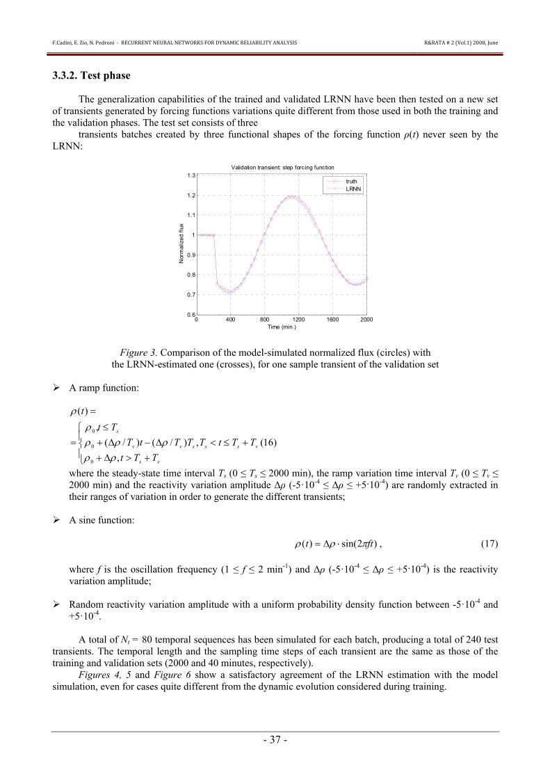
FCadini E Zio N Pedroni ‐ RECURRENT NEURAL NETWORKS FOR DYNAMIC RELIABILITY ANALYSIS
RampRATA 2 (Vol1) 2008 June
- 40 -
[11] Haykin S (1994) Neural networks a comprehensive foundation New York IEEE Press [12] Hochreiter S amp Schmidhuber J (1997) Long short-term memory Neural Computation 9(8) 1735-
1780 [13] Izquierdo JM Hortal J Sanchez-Perea M amp Melendez E (1994) Automatic Generation of dynamic
Event Trees A Tool for Integrated Safety Assessment (ISA) Reliability and Safety Assessment of Dynamic Process System NATO-ASI Series F Vol 120 Springer-Verlag Berlin
[14] Labeau P E amp Zio E (1998) The Cell-to-Boundary Method in the Frame of Memorization-Based Monte Carlo Algorithms A New Computational Improvement in Dynamic Reliability Mathematics and Computers in Simulation Vol 47 No 2-5 329-347
[15] Labeau PE (1996) Probabilistic Dynamics Estimation of Generalized Unreliability Trhough Efficient Monte Carlo Simulation Annals of Nuclear Energy Vol 23 No 17 1355-1369
[16] Marseguerra M amp Zio E (1996) Monte Carlo approach to PSA for dynamic process systems Reliab Eng amp System Safety vol 52 227-241
[17] Narendra K S amp Parthasarathy K (1990) Identification and control of dynamical systems using neural networks IEEE Trans Neural Networks 1 4-27
[18] Pearlmutter B (1995) Gradient Calculations for Dynamic Recurrent Neural networks a Survey IEEE Trans Neural Networks 6 1212
[19] Siegelmann H amp Sontag E (1995) On the Computational Power of Neural Nets J Computers and Syst Sci 50 (1) 132
[20] Siu N (1994) Risk Assessment for Dynamic Systems An Overview Reliab Eng amp System Safety vol 43 43-74
FCadini E Zio N Pedroni ‐ RECURRENT NEURAL NETWORKS FOR DYNAMIC RELIABILITY ANALYSIS
RampRATA 2 (Vol1) 2008 June
- 41 -
Appendix the Recursive Back-Propagation (RBP) Algorithm for batch training
Consider one training temporal sequence of length T and denote by dr(t) r = 1 2 hellip NM the desired output value of the training sequence at time t
The instantaneous squared error at time t e2(t) is defined as the sum over all NM output nodes of the squared deviations of the network outputs xM
r(t) from the corresponding desired value in the training temporal sequence dr(t)
[ ]sum=
=MN
rr tete
1
22 )()( (1rsquo)
where )()()( txtdte M
rrr minus= (2rsquo)
The training algorithm aims at minimizing the global squared error E2 over the whole training sequence of length T
sum=
=T
t
teE1
22 )( (3rsquo)
This is achieved by modifying iteratively the network weights wk
jl(p) vkjl(p) along the gradient descent
viz
2
2
)(
2
)(
)(
2
)(
kpjl
kpjl
kpjl
kpjl
vEv
wEw
partpart
minus=Δ
partpart
minus=Δ
μ
μ
(4rsquo)
where μ is the learning rate Introducing the usual backpropagating error and delta quantities with respect to the output xk
j(t) and input sk
j(t) of the generic node j of layer k
)(2
1)(2
txEte kj
kj part
partminus= (5rsquo)
[ ])()(
)(
)(
)(21
)(21)(
22
tsfte
ts
tx
txE
tsEt
kjk
kj
kj
kj
kj
kj
kj
=
part
part
partpart
minus=partpart
minus=δ
(6rsquo)
the chain rule for the modification (4rsquo) of the MA and AR synaptic weights wk
jl(p) vkjl(p) can be written as
)(
)(
)()(
2
)(1
1)(
2
)(
kpjl
kj
T
t
kj
T
t
kpjl
kj
kj
kpjl
wts
t
wts
tsE
w
part
part=
part
part
partpart
minus=Δ
sum
sum
=
=
μδ
μ
FCadini E Zio N Pedroni ‐ RECURRENT NEURAL NETWORKS FOR DYNAMIC RELIABILITY ANALYSIS
RampRATA 2 (Vol1) 2008 June
- 42 -
)(
)(
)()(2
)(1
1 )(
2
)(
kpjl
kj
T
t
kj
T
tk
pjl
kj
kj
kpjl
vts
t
vts
tsEv
part
part=
part
part
partpart
minus=Δ
sum
sum
=
=
μδ
μ
(7rsquo)
Note that the weights updates (7rsquo) are performed in batch at the end of the training sequence of length
T From (10)
)()(
)()(
)()()()(k
pjl
kjl
kpjl
kj
kpjl
kjl
kpjl
kj
v
ty
v
ts
w
ty
w
ts
part
part=
part
part
part
part=
part
part (8rsquo)
so that from the differentiation of (11) one obtains
)(
)()(
)(1)(
1
)(k
pjl
kj
kjlI
kjl
klk
pjl
kj
w
tsvptx
w
ts
part
minuspartsum+minus=
part
part
=
minus ττ
τ (9rsquo)
)(
)()(
)(1)(
)(k
pjl
kj
kjlI
kjl
kjlk
pjl
kj
v
tsvpty
v
ts
part
minuspartsum+minus=
part
part
=
ττ
τ (10rsquo)
To compute δk
j(t) from (6rsquo) we must be able to compute ekj(t) Applying the chain rule to (5rsquo) one has
sum sumpart
part
partpart
minus=+
= =
+
+
1
1 1
1
1
2
)(
)(
)(21)(
kN
q
T
kj
kq
kq
kj tx
s
sEte
τ
τ
τ Mk lt (11rsquo)
Under the hypothesis of synaptic filter temporal causality (according to which the state of a node at
time t influences the network evolution only at successive times and not at previous ones) the summation along the time trajectory can start from τ = t Exploiting the definitions (6rsquo) and (8rsquo) changing the variables as τ ndash p t and considering that for the output layer ie k = M the derivative partE2partxM
j(t) can be computed directly from (2rsquo) the back-propagation of the error through the layers can be derived
⎪⎪
⎩
⎪⎪
⎨
⎧
sum sum ltpart
+part+
=
=minus
=
+
=
++tT
p
kN
q kj
kqik
q
j
kj
Mktx
ptypt
Mkeqte
te
0
1
1
11
)(
)()(
)2()(
)(δ
(12rsquo)
where from (11)
⎩⎨⎧ minuslele
+
sumpart
minus+part=
part
+part
++
+
=
++
+
010
)(
)(
)(
)(
11)(
)1min(
1
11
)(
1
otherwiseLpw
tx
ptyv
tx
pty
kqj
kpqj
pkqjI
kj
kqjk
qjkj
kqj
ττ
τ
(13rsquo)
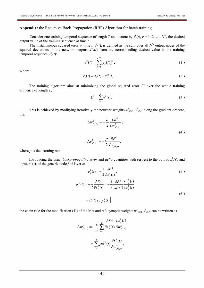
FCadini E Zio N Pedroni ‐ RECURRENT NEURAL NETWORKS FOR DYNAMIC RELIABILITY ANALYSIS
RampRATA 2 (Vol1) 2008 June
- 42 -
)(
)(
)()(2
)(1
1 )(
2
)(
kpjl
kj
T
t
kj
T
tk
pjl
kj
kj
kpjl
vts
t
vts
tsEv
part
part=
part
part
partpart
minus=Δ
sum
sum
=
=
μδ
μ
(7rsquo)
Note that the weights updates (7rsquo) are performed in batch at the end of the training sequence of length
T From (10)
)()(
)()(
)()()()(k
pjl
kjl
kpjl
kj
kpjl
kjl
kpjl
kj
v
ty
v
ts
w
ty
w
ts
part
part=
part
part
part
part=
part
part (8rsquo)
so that from the differentiation of (11) one obtains
)(
)()(
)(1)(
1
)(k
pjl
kj
kjlI
kjl
klk
pjl
kj
w
tsvptx
w
ts
part
minuspartsum+minus=
part
part
=
minus ττ
τ (9rsquo)
)(
)()(
)(1)(
)(k
pjl
kj
kjlI
kjl
kjlk
pjl
kj
v
tsvpty
v
ts
part
minuspartsum+minus=
part
part
=
ττ
τ (10rsquo)
To compute δk
j(t) from (6rsquo) we must be able to compute ekj(t) Applying the chain rule to (5rsquo) one has
sum sumpart
part
partpart
minus=+
= =
+
+
1
1 1
1
1
2
)(
)(
)(21)(
kN
q
T
kj
kq
kq
kj tx
s
sEte
τ
τ
τ Mk lt (11rsquo)
Under the hypothesis of synaptic filter temporal causality (according to which the state of a node at
time t influences the network evolution only at successive times and not at previous ones) the summation along the time trajectory can start from τ = t Exploiting the definitions (6rsquo) and (8rsquo) changing the variables as τ ndash p t and considering that for the output layer ie k = M the derivative partE2partxM
j(t) can be computed directly from (2rsquo) the back-propagation of the error through the layers can be derived
⎪⎪
⎩
⎪⎪
⎨
⎧
sum sum ltpart
+part+
=
=minus
=
+
=
++tT
p
kN
q kj
kqik
q
j
kj
Mktx
ptypt
Mkeqte
te
0
1
1
11
)(
)()(
)2()(
)(δ
(12rsquo)
where from (11)
⎩⎨⎧ minuslele
+
sumpart
minus+part=
part
+part
++
+
=
++
+
010
)(
)(
)(
)(
11)(
)1min(
1
11
)(
1
otherwiseLpw
tx
ptyv
tx
pty
kqj
kpqj
pkqjI
kj
kqjk
qjkj
kqj
ττ
τ
(13rsquo)
Related Documents