Reconstruction of secular variation in seawater sulfate concentrations (2014, Biogeosciences Discussions)

BGD11, 13187–13250, 2014

Reconstruction ofseawater sulfate

T. J. Algeo et al.

Title Page

Abstract Introduction

Conclusions References

Tables Figures

J I

J I

Back Close

Full Screen / Esc

Printer-friendly Version

Interactive Discussion

Discussion

Paper

|D

iscussionP

aper|

Discussion

Paper

|D

iscussionP

aper|

Biogeosciences Discuss., 11, 13187–13250, 2014www.biogeosciences-discuss.net/11/13187/2014/doi:10.5194/bgd-11-13187-2014© Author(s) 2014. CC Attribution 3.0 License.

This discussion paper is/has been under review for the journal Biogeosciences (BG).Please refer to the corresponding final paper in BG if available.

Reconstruction of secular variation inseawater sulfate concentrationsT. J. Algeo1,2,3, G. M. Luo2,3, H. Y. Song3, T. W. Lyons4, and D. E. Canfield5

1Department of Geology, University of Cincinnati, Cincinnati, Ohio 45221-0013, USA2State Key Laboratory of Geological Processes and Mineral Resources, China University ofGeosciences, Wuhan, 430074, China3State Key Laboratory of Biogeology and Environmental Geology, China University ofGeosciences, Wuhan, 430074, China4Department of Earth Sciences, University of California, Riverside, California 92521-0423,USA5Nordic Center for Earth Evolution (NordCEE) and Institute of Biology, University of SouthernDenmark, Campusvej 55, 5230 Odense M, Denmark

Received: 26 July 2014 – Accepted: 23 August 2014 – Published: 10 September 2014

Correspondence to: T. J. Algeo ([email protected])

Published by Copernicus Publications on behalf of the European Geosciences Union.

13187

http://www.biogeosciences-discuss.net

http://www.biogeosciences-discuss.net/11/13187/2014/bgd-11-13187-2014-print.pdf

http://www.biogeosciences-discuss.net/11/13187/2014/bgd-11-13187-2014-discussion.html

http://creativecommons.org/licenses/by/3.0/

BGD11, 13187–13250, 2014


T. J. Algeo et al.

Title Page



Tables Figures

J I

J I

Back Close

Full Screen / Esc



Discussion

Paper

|D

iscussionP

aper|

Discussion

Paper

|D

iscussionP

aper|

Abstract

Long-term secular variation in seawater sulfate concentrations ([SO2−4 ]SW) is of inter-

est owing to its relationship to the oxygenation history of Earth’s surface environment,but quantitative approaches to analysis of this variation remain underdeveloped. In thisstudy, we develop two complementary approaches for assessment of the [SO2−

4 ] of an-5

cient seawater and test their application to reconstructions of [SO2−4 ]SW variation since

the late Neoproterozoic Eon (<650 Ma). The first approach is based on two measurableparameters of paleomarine systems: (1) the S-isotope fractionation associated with mi-crobial sulfate reduction (MSR), as proxied by ∆34SCAS-PY, and (2) the maximum rateof change in seawater sulfate, as proxied by ∂δ34SCAS/∂t (max). This “rate method”10

yields an estimate of the maximum possible [SO2−4 ]SW for the time interval of inter-

est, although the calculated value differs depending on whether an oxic or an anoxicocean model is inferred. The second approach is also based on ∆34SCAS-PY but eval-uates this parameter against an empirical MSR trend rather than a formation-specific∂δ34SCAS/∂t (max) value. The MSR trend represents the relationship between frac-15

tionation of cogenetic sulfate and sulfide (i.e., ∆34Ssulfate-sulfide) and ambient dissolvedsulfate concentrations in 81 modern aqueous systems. This “MSR-trend method” isthought to yield a robust estimate of mean seawater [SO2−

4 ] for the time interval ofinterest. An analysis of seawater sulfate concentrations since 650 Ma suggests that[SO2−

4 ]SW was low during the late Neoproterozoic (< 5 mM), rose sharply across the20

Ediacaran/Cambrian boundary (to ∼ 5–10 mM), and rose again during the Permian tolevels (∼10–30 mM) that have varied only slightly since 250 Ma. However, Phanerozoicseawater sulfate concentrations may have been drawn down to much lower levels (∼1–4 mM) during short (.2 Myr) intervals of the Cambrian, Early Triassic, Early Jurassic,and possibly other intervals as a consequence of widespread ocean anoxia, intense25

MSR, and pyrite burial. The procedures developed in this study offer potential for futurehigh-resolution quantitative analyses of paleoseawater sulfate concentrations.

13188





BGD11, 13187–13250, 2014


T. J. Algeo et al.

Title Page



Tables Figures

J I

J I

Back Close

Full Screen / Esc



Discussion

Paper

|D

iscussionP

aper|

Discussion

Paper

|D

iscussionP

aper|

1 Introduction

Oceanic sulfate plays a key role in the biogeochemical cycles of S, C, O and Fe (Can-field, 1998; Lyons and Gill, 2010; Halevy et al., 2012; Planavsky et al., 2012). Forexample, > 50 % of organic matter and methane in marine sediments is oxidized viaprocesses linked to microbial sulfate reduction (MSR) (Jørgensen, 1982; Valentine,5

2002). At a concentration of ∼ 29 mM in the modern ocean, sulfate is the second mostabundant anion in seawater (Millero, 2005). Its concentration is an important proxy forseawater chemistry and the oxidation state of the Earth’s atmosphere and oceans (Kahet al., 2004; Johnston, 2011).

Although there is broad agreement that seawater sulfate concentrations have in-10

creased through time, the history of its accumulation remains poorly known in de-tail. Archean and Early Proterozoic oceans are thought to have had very limited sul-fate inventories (< 200 µM), as implied by small degrees of sulfate-sulfide and mass-independent S-isotope fractionation (Shen et al., 2001; Strauss, 2003; Farquhar et al.,2007; Adams et al., 2010; Johnston, 2011; Owens et al., 2013; Luo et al., 2014).15

The accumulation of atmospheric O2 during Great Oxidation Event (GOE) I (∼ 2.3–2.0 Ga; Holland, 2002; Bekker et al., 2004; Guo et al., 2009) is thought to have resultedin a long-term increase in seawater sulfate concentrations (Canfield and Raiswell,1999; Canfield et al., 2007; Kah et al., 2004; Fike et al., 2006; Schröder et al., 2008;Planavsky et al., 2012; Reuschel et al., 2012). However, this increase was probably20

not monotonic and declines in pO2 may have resulted in one or more seawater sulfateminima between ∼ 1.9 and 0.6 Ga (Planavsky et al., 2012; Luo et al., 2014). Estimatesof Phanerozoic seawater sulfate concentrations are uniformly higher, although there isno consensus regarding exact values. Fluid inclusion data yielded estimates of ∼ 10to 30 mM for most of the Phanerozoic (Horita et al., 2002; Lowenstein et al., 2003).25

However, recent S-isotope studies have modeled concentrations as low as ∼ 1–5 mMduring portions of the Cambrian, Triassic, Jurassic, and Cretaceous (Wortmann andChernyavsky, 2007; Adams et al., 2010; Luo et al., 2010; Gill et al., 2011a, b; Newton

13189





BGD11, 13187–13250, 2014


T. J. Algeo et al.

Title Page



Tables Figures

J I

J I

Back Close

Full Screen / Esc



Discussion

Paper

|D

iscussionP

aper|

Discussion

Paper

|D

iscussionP

aper|

et al., 2011; Owens et al., 2013; Song et al., 2014), and a recent marine S-cycle modelyielded low concentrations (< 10 mM) for the entire Cretaceous and Early Cenozoicbefore a rise to near-modern levels at ∼ 40 Ma (Wortmann and Paytan, 2012).

Here, we develop two approaches for quantitative analysis of seawater sulfate con-centrations ([SO2−

4 ]SW) in paleomarine systems. The first method calculates a maxi-5

mum possible [SO2−4 ]SW based on a combination of two parameters that are readily

measurable in most paleomarine systems: (1) the S-isotope fractionation between co-genetic sedimentary sulfate and sulfide (∆34SCAS-PY), and (2) the maximum observedrate of variation in seawater sulfate δ34S (∂δ34SCAS/∂t). This “rate method” is an ex-tension of earlier modeling work by Kump and Arthur (1999), Kurtz et al. (2003), Kah10

et al. (2004), Bottrell and Newton (2006), and Gill et al. (2011a, b). The second ap-proach yields an estimate of mean seawater [SO2−

4 ] based on an empirical relationship

between ∆34SCAS-PY and ambient dissolved sulfate concentrations in 81 modern aque-ous systems (the MSR trend). This “MSR-trend method” is thus based on an updatedversion of the fractionation relationship that was quantified by Habicht et al. (2002;15

their Fig. 1). Whereas earlier analyses commonly made qualitative assessments ofpaleo-seawater [SO2−

4 ] (e.g., Chu et al., 2007), the significance of our methodology is

that the [SO2−4 ] of ancient seawater can be quantitatively constrained as a function of

measurable sediment parameters and empirical fractionation relationships.We fully recognize that the marine sulfur cycle is controlled by myriad factors, many20

of which are only now coming to light thanks to detailed field and laboratory studies,and that not all such influences can be thoroughly considered and accommodated inthe present study. While acknowledging the complexity of the sulfur cycle, this paperattempts to identify broad first-order trends that potentially transcend these diverseinfluences and that are robust over significant intervals of geologic time. Our ultimate25

goal is to generate useful approximations of the long-term history of sulfate in theocean. Our results suggest that large-scale empirical relationships may exist that arenot highly sensitive to local controls such as rates of MSR, syngenetic vs. diageneticpyrite formation, and strain-specific isotopic behavior, among others. We envision such

13190





BGD11, 13187–13250, 2014


T. J. Algeo et al.

Title Page



Tables Figures

J I

J I

Back Close

Full Screen / Esc



Discussion

Paper

|D

iscussionP

aper|

Discussion

Paper

|D

iscussionP

aper|

local influences, as they become more completely understood, being mapped onto,and thus integrated with, the broad first-order relationships documented herein.

2 Methods of modeling paleo-seawater sulfate concentrations

2.1 The rate method

The marine S cycle has a limited number of fluxes with well-defined S-isotope ranges5

(Holser et al., 1989; Canfield, 2004; Bottrell and Newton, 2006) and, thus, is amenableto analysis through modeling (e.g., Halevy et al., 2012). Subaerial weathering yieldsa riverine sulfate source flux (FQ) of ∼ 10×1013 g yr−1 with an average δ34S of ∼ +6 ‰,which is significantly lighter than the modern seawater sulfate δ34S of +20 ‰. Sulfateis removed to the sediment either in an oxidized state, as carbonate-associated sul-10

fate (CAS) or evaporite deposits, or in a reduced state, mainly as FeS or FeS2. Theoxidized sink has a flux (FEVAP) of ∼ 6×1013 g yr−1 with a S-isotopic composition thatclosely mimics that of coeval seawater (∆34SSW-EVAP of −4 to 0 ‰). The reduced sinkhas a flux (FPY) of ∼ 4×1013 g yr−1 with a composition that characteristically showsa large negative fractionation relative to coeval seawater (∆34SSW-PY of ∼ 30 to 60 ‰;15

Habicht and Canfield, 1997). Secular variation in seawater sulfate δ34S is mainly dueto changes in the relative size of the sink fluxes, with increasing (decreasing) burial ofpyrite relative to sulfate leading to more (less) 34S-enriched seawater sulfate (Holseret al., 1989; Bottrell and Newton, 2006; Halevy et al., 2012).

We adapted the models of Kurtz et al. (2003) and Kah et al. (2004) in order to20

calculate ancient seawater sulfate concentrations ([SO2−4 ]SW) based on two param-

eters: (1) S-isotope fractionation between cogenetic sedimentary sulfate and sul-fide (∆34Ssulfate-sulfide, as proxied by ∆34SCAS-PY), and (2) the maximum observedrate of variation in seawater sulfate S isotopes (∂δ34SSO4

/∂t(max), as proxied by

∂δ34SCAS/∂t(max)) (Fig. 1). Rates of isotopic change for seawater sulfate are given25

13191





BGD11, 13187–13250, 2014


T. J. Algeo et al.

Title Page



Tables Figures

J I

J I

Back Close

Full Screen / Esc



Discussion

Paper

|D

iscussionP

aper|

Discussion

Paper

|D

iscussionP

aper|

by:

∂δ34SCAS/∂t =((

FQ ×∆34SQ-SW

)−(FPY ×∆34SCAS-PY

))/MSW (1)

where FQ×∆34SQ-SW is the flux-weighted difference in the isotopic compositions of thesource flux and seawater (SW), FPY ×∆34SCAS-PY is the flux-weighted difference in the5

isotopic compositions of the reduced-S sink flux and seawater, and MSW is the massof seawater sulfate. The full expression represents the time-integrated influence of thesource and sink fluxes on seawater sulfate δ34S. The maximum possible rate of changein the sulfur isotopic composition of seawater sulfate is attained when one of the fluxes(e.g., the source flux, as in Eq. 2) goes to zero:10

∂δ34SCAS/∂t(max) = FPY ×∆34SCAS-PY/MSW (2)

Reorganization of this equation allows calculation of a maximum seawater sulfate con-centration from measured values of ∆34SCAS-PY and ∂δ34SCAS/∂t(max):

MSW = k1 × FPY ×∆34SCAS-PY/(∂δ34SCAS/∂t(max)

)(3)15 [

SO2−4

]SW

(max) = k2 ×MSW (4)

where k1 is a unit-conversion constant equal to 106, and k2 is a constant relating themass of seawater sulfate to its molar concentration that is equal to 2.15×10−20 mM g−1.Kah et al. (2004) used FPY = 10×1013 g yr−1, which is the total sink flux for modern20

seawater sulfate, in order to model ∂δ34SCAS/∂t(max). While this may be appropriatefor intervals of widespread euxinia in the global ocean, FPY = 4×1013 g yr−1 (i.e., themodern value) may better represent intervals with well-oxygenated oceans in whichthe sinks of sulfate S and pyrite S are subequal (Fig. 1). For values of ∆34SCAS-PY and∂δ34SCAS/∂t(max) that are potentially representative of the modern ocean (e.g., 35 ‰25

13192





BGD11, 13187–13250, 2014


T. J. Algeo et al.

Title Page



Tables Figures

J I

J I

Back Close

Full Screen / Esc



Discussion

Paper

|D

iscussionP

aper|

Discussion

Paper

|D

iscussionP

aper|

and 1.1 ‰ Myr−1; see discussion below), Eq. (3) yields the modern seawater sulfatemass of MSW = 1.3×1021 g (assuming FPY = 4×1013 g yr−1), and Eq. (4) yields themodern seawater sulfate concentration of ∼ 29 mM (Millero, 2005).

Relationships among the model parameters are illustrated in Fig. 1 for ∆34SCAS-PY

from 1 to 100 ‰ (ordinal scale) and for discrete values of ∂δ34SCAS/∂t(max) ranging5

from 1 to 100 ‰ Myr−1 (diagonal lines). [SO2−4 ]SW increases linearly with increasing

∆34SCAS-PY (at constant ∂δ34SCAS/∂t(max)) and decreases linearly with increasing∂δ34SCAS/∂t(max) (at constant ∆34SCAS-PY). The observed maximum ∂δ34SCAS/∂tis generally smaller than the theoretical maximum ∂δ34SSO4

/∂t because the lattercan be achieved only when the source flux of seawater sulfate is reduced (at least10

transiently) to zero (Kah et al., 2004), which does not routinely occur in nature. Asa consequence, estimates of [SO2−

4 ]SW for a given paleomarine system generally arelarger than actual seawater sulfate concentrations, so Eq. (4) yields the maximumlikely [SO2−

4 ]SW for an interval of interest. This outcome is illustrated by a calculation

for the modern ocean, using ∆34SCAS-PY of ∼ 30–60 ‰ (e.g., Canfield and Thamdrup,15

1994) and ∂δ34SCAS/∂t(max) of ∼ 0.5 ‰ Myr−1 (based on the Cenozoic seawater sul-fate δ34S record; Paytan et al., 1998). These inputs yield [SO2−

4 ]SW (max) values be-

tween ∼ 40 and 120 mM, which is modestly larger than the actual modern [SO2−4 ]SW

of ∼ 29 mM (Fig. 1). Overestimation of modern [SO2−4 ]SW is due to the fact that ob-

served ∂δ34SCAS/∂t values for the Cenozoic are just < 0.5 ‰ Myr−1 and, thus, have20

not approached the theoretical maximum for modern seawater (∼ 1–2 ‰ Myr−1; Fig. 1).This situation is probably typical of the marine sulfur cycle through time – maximum ob-served rates of ∂δ34SCAS/∂t are generally going to be lower than maximum theoreticalrates because the source flux of sulfur to the oceans has probably never gone to zero(as modeled in Eq. 2).25

13193





BGD11, 13187–13250, 2014


T. J. Algeo et al.

Title Page



Tables Figures

J I

J I

Back Close

Full Screen / Esc



Discussion

Paper

|D

iscussionP

aper|

Discussion

Paper

|D

iscussionP

aper|

2.2 The MSR-trend method

An alternative approach to constraining ancient seawater sulfate concentrations isbased on empirical relationships with the S-isotope fractionation associated withmicrobial sulfate reduction (FMSR). We evaluated this relationship by compiling∆34Ssulfate-sulfide and [SO2−

4 ]aq data for 81 examples from modern aqueous systems,5

including freshwater, brackish, marine, and hypersaline environments (Table A1; cf.Habicht et al., 2002). Each system was classified (1) by salinity, as freshwater(< 10 psu), brackish (10–30 psu), marine (30–40 psu), or hypersaline (> 40 psu; n.b.,psu=practical salinity units), and (2) by redox conditions, as oxic or euxinic dependingon whether the chemocline was within the sediment or the watermass, respectively.10

In the interests of applying uniform criteria to the generation of this dataset, wefollowed a specific protocol. First, we used only in-situ water-column measurementsof δ34S for aqueous sulfate. Second, we used in-situ water-column or uppermostsediment-porewater measurements of δ34S for aqueous sulfide or, if lacking, mea-surements of δ34S of sedimentary sulfide as a proxy for aqueous sulfide. Because15

solid-phase sulfides generally exhibit a pronounced shift toward more 34S-enrichedcompositions under sulfate-limited (e.g., burial) conditions, we used δ34S values onlyfrom samples taken at or within a few centimeters of the sediment-water interface.Some variation in δ34S among cogenetic sedimentary sulfides is common. Pyrite S isgenerally more 34S-depleted than acid-volatile S (AVS) and organic S because it repre-20

sents a time-integrated signal that incorporates early-generated, strongly 34S-depletedH2S (Kaplan et al., 1963; Canfield et al., 1992). On the other hand, AVS tends to havea heavier sulfur isotopic composition, closer to that of the instantaneously generatedH2S at a given sediment depth, because it converts quickly to pyrite with burial (Lyons,1997), and organic S tends to be isotopically heavier possibly owing to fractionations25

associated with the sulfurization of organic matter (Werne et al., 2000, 2003, 2008).For these reasons, we utilized pyrite rather than AVS or other solid-phase sulfides asa proxy in estimating aqueous sulfide δ34S. Third, we adopted a modern seawater

13194





BGD11, 13187–13250, 2014


T. J. Algeo et al.

Title Page



Tables Figures

J I

J I

Back Close

Full Screen / Esc



Discussion

Paper

|D

iscussionP

aper|

Discussion

Paper

|D

iscussionP

aper|

sulfate concentration of 2775 mg L−1 or 28.9 mM (given a seawater density of 1025 kgm−3) (Millero, 2005). For non-marine settings, we used measured aqueous sulfate con-centrations wherever available. Where unavailable for brackish or hypersaline marinesystems, we calculated dissolved sulfate concentration from salinity data:[SO2−

4

]=[SO2−

4

]SW

×S/SSW (5)5

where [SO2−4 ] and S are the sulfate concentration and salinity of the watermass of in-

terest, respectively, and SSW is the salinity of average seawater (35 psu). Some secularvariation in the salinity and, hence, aqueous sulfate concentration of non-marine andrestricted-marine watermasses is likely, but its potential effect on the FMSR-[SO2−

4 ]aq10

relationship may be limited.The protocol above produced an internally consistent dataset (Table A1) that exhibits

a pronounced relationship between ∆34Ssulfate-sulfide and [SO2−4 ]aq (Fig. 2a). Regression

of ∆34Ssulfate-sulfide on [SO2−4 ]aq yields a linear relationship with a strong positive corre-

lation (r2 = 0.80). The trend represents an increase in ∆34Ssulfate-sulfide from ∼ 4–6 ‰15

at 0.1 mM to ∼ 30–60 ‰ at 29 mM (i.e., modern seawater [SO2−4 ]). ∆34Ssulfate-sulfide

appears to peak at [SO2−4 ]aq of 15–20 mM, with a mean value ∼ 5–10 ‰ greater

than for [SO2−4 ]SW, but this effect is small relative to the overall relationship between

∆34Ssulfate-sulfide and [SO2−4 ]aq, and we did not factor it separately into the regression

analysis. For hypersaline environments in which [SO2−4 ]aq > 29 mM, ∆34Ssulfate-sulfide20

does not continue to rise but, rather, shows roughly the same range as for modernseawater (Fig. 2a). Finally, we analyzed the data by redox environment and foundonly minor and statistically insignificant differences between oxic and euxinic settings(n.b., hypersaline environments were not included in this analysis). The distributionsof the oxic and euxinic datasets show broad overlap (Fig. 2a), so benthic redox condi-25

tions appear to exhibit no discernible influence on the relationship of ∆34Ssulfate-sulfide to[SO2−

4 ]aq.13195





BGD11, 13187–13250, 2014


T. J. Algeo et al.

Title Page



Tables Figures

J I

J I

Back Close

Full Screen / Esc



Discussion

Paper

|D

iscussionP

aper|

Discussion

Paper

|D

iscussionP

aper|

Our analysis demonstrates that a strong relationship exists between FMSR and[SO2−

4 ]aq in natural aqueous systems (r2 = 0.80; Fig. 2a). Our results are similar to,although more linear and more statistically robust than, those reported by Habichtet al. (2002) on the basis of culture experiments. We recognize that there are multi-ple environmental and physiological controls on fractionation by sulfate reducers (see5

discussion below), and that under certain natural and experimental conditions the re-lationship of FMSR to [SO2−

4 ]aq can deviate markedly from that in our dataset. However,

the pattern of covariation between FMSR and [SO2−4 ]aq documented here represents

a robust relationship that appears to hold for a wide range of natural environments, re-flecting a widespread and possibly ubiquitous influence of [SO2−

4 ]aq on FMSR. Nonethe-10

less, the strength of the FMSR-[SO2−4 ]aq relationship shown in Fig. 2a suggests that it

can serve as a basis for evaluating the [SO2−4 ]aq of ancient seawater. Seawater [SO2−

4 ]

can be estimated graphically by projecting measured values of ∆34SCAS-PY from theordinal scale to the MSR trend and then to the abscissa (Fig. 2b), or by using thefollowing empirical equation:15 [SO2−

4

]= 0.42×∆34SCAS-PY −0.15 (6)

The upper and lower uncertainty limits for estimates of seawater [SO2−4 ] based on this

relationship are:[SO2−

4

]= 0.40×∆34SCAS-PY −0.02 (upper limit) (7)20 [

SO2−4

]= 0.44×∆34SCAS-PY −0.28 (lower limit) (8)

In order to account for uncertainties in ∆34SCAS-PY as well as the FMSR regression,estimates of minimum [SO2−

4 ]SW should make use of minimum ∆34SCAS-PY values incombination with the upper uncertainty limit equation (Eq. 7), and estimates of maxi-25

mum [SO2−4 ]SW should make use of maximum ∆34SCAS-PY values in combination with

the lower uncertainty limit equation (Eq. 8; Fig. 2b).13196





BGD11, 13187–13250, 2014


T. J. Algeo et al.

Title Page



Tables Figures

J I

J I

Back Close

Full Screen / Esc



Discussion

Paper

|D

iscussionP

aper|

Discussion

Paper

|D

iscussionP

aper|

3 Controls on fractionation by microbial sulfate reducers

The biogeochemical nature of the microbial sulfate reduction (MSR) process and itsassociated S-isotope fractionations have been extensively investigated in earlier stud-ies. Sulfate reducers preferentially utilize sulfate containing 32S during dissimilatoryreduction to hydrogen sulfide in conjunction with the anaerobic decay of organic matter5

(Kaplan, 1983; Canfield, 2001; Bradley et al., 2011). The exact controls on this iso-topic discrimination continue to be a topic of intense debate. The paradigmatic view isthat this fractionation is mainly a kinetic effect associated with the rate-limiting step forintracellular sulfate processing, although it is known that fractionation also may accom-pany sulfate transport across the cell membrane (Rees, 1973; Detmers et al., 2001;10

Brüchert, 2004; Bradley et al., 2011). The kinetic effect is thought to be dependenton aqueous sulfate concentrations, with substantially larger fractionations associatedwith [SO2−

4 ]aq & 200 µM (Habicht et al., 2002; Gomes and Hurtgen, 2013; but see Can-field, 2001, for a counter example). Rees (1973) proposed a maximum discrimina-tion of 46 ‰ but the theoretical basis for this value was re-assessed by Brunner and15

Bernasconi (2005). Recent studies have documented FMSR as large as 66 ‰ in cultureexperiments (Sim et al., 2011a) and 72 ‰ in natural systems (Wortmann et al., 2001;Canfield et al., 2010). Even larger fractionations have been reported but are generallyconsidered to be the result of multistage disproportionation of intermediate-oxidation-state sulfur compounds (Canfield and Thamdrup, 1994).20

Investigations of natural and experimental systems have documented a number ofadditional controls on FMSR. One of the most important controls is fSO4

, i.e., the fractionof remaining dissolved sulfate (Gomes and Hurtgen, 2013). In “open systems” contain-ing a high concentration of dissolved sulfate (e.g., the modern ocean), fSO4

does notvary measurably from 1.0 because the quantity of sulfate converted to sulfide via MSR25

is a small fraction of the total aqueous sulfate inventory. In this case, the produced sul-fide will show the maximum degree of fractionation, which is typically ∼ 30 to 60 ‰ inmodern marine systems (Habicht and Canfield, 1997; Fig. 2a). In contrast, in “closed

13197





BGD11, 13187–13250, 2014


T. J. Algeo et al.

Title Page



Tables Figures

J I

J I

Back Close

Full Screen / Esc



Discussion

Paper

|D

iscussionP

aper|

Discussion

Paper

|D

iscussionP

aper|

systems” in which the aqueous sulfate inventory is limited (e.g., sediment porewaters orlow-sulfate freshwater systems), dissolved sulfate concentrations can be substantiallyreduced or completely depleted through MSR, causing fSO4

to evolve toward zero. As

[SO2−4 ]aq becomes smaller, sulfate reducers utilize a progressively larger fraction of the

total dissolved sulfate pool, reducing the effective fractionation to small values (Habicht5

et al., 2002; Gomes and Hurtgen, 2013). In these settings, the aggregate δ34S compo-sition of the produced sulfide approaches that of the original aqueous sulfate inventory,and ∆34Ssulfate-sulfide approaches zero (Kaplan, 1983; Habicht et al., 2002). In a macrosense, fSO4

can be proxied by [SO2−4 ]aq, accounting for the strong first-order relation-

ship between the latter parameter and ∆34Ssulfate-sulfide (r2 = 0.80; Fig. 2a). However,10

not all researchers agree on the importance of fSO4as a control on FMSR (e.g., Leavitt

et al., 2013).Other factors may influence FMSR under certain conditions. First, different dissimi-

latory reduction pathways yield different isotopic discriminations. Oxidation of organicsubstrates to CO2 yields larger fractionations (∼ 30–60 ‰) than oxidation to acetate15

(< 18 ‰) (Detmers et al., 2001; Brüchert et al., 2001; Brüchert, 2004). Incomplete ox-idation of organic substrates is a feature characteristic of sulfate reducers in hyper-saline environments (Habicht and Canfield, 1997; Oren, 1999; Detmers et al., 2001;Stam et al., 2010) and may account for the somewhat smaller fractionations typicallyencountered in such environments (Fig. 2a). Second, the type of organic substrate20

also matters, as ethanol, lactate, glucose, and other compounds yielded a range offractionations under otherwise similar conditions (Canfield, 2001; Detmers et al., 2001;Kleikemper et al., 2004; Sim et al., 2011b). Third, sulfate reduction rates may alsoinfluence FMSR, with higher rates associated with smaller isotopic discriminations (Ka-plan and Rittenberg, 1964; Kemp and Thode, 1968; Chambers et al., 1975; Habicht25

and Canfield, 1996; Brüchert et al., 2001; Canfield, 2001). Recent experiments byLeavitt et al. (2013) showed that FMSR declines rapidly with increasing sulfate reduc-tion rates before leveling off at ∼ 15–20 ‰ at rates > 50 mmol H2S per unit substrateper day. Habicht and Canfield (2001) hypothesized that FMSR is only incidentally re-

13198





BGD11, 13187–13250, 2014


T. J. Algeo et al.

Title Page



Tables Figures

J I

J I

Back Close

Full Screen / Esc



Discussion

Paper

|D

iscussionP

aper|

Discussion

Paper

|D

iscussionP

aper|

lated to sulfate reduction rates because both are correlated with the disproportionationof intermediate-oxidation-state S compounds by sulfur-oxidizing bacteria, which haveprobably been present since the Archean (Johnston et al., 2005; Wacey et al., 2010).Finally, temperature has been shown to affect FMSR in some studies (e.g., Canfieldet al., 2006) but not others (e.g., Detmers et al., 2001). The influence of temperature on5

FMSR may operate through the species-specific temperature dependence of enzymes.Research to date clearly shows that controls on microbial sulfate reduction are com-

plex and incompletely understood. This situation reflects the diverse composition ofthe microbial communities that process sulfur in the marine environment and the rangeof isotopic fractionations associated with those processes (Brüchert, 2004). Yet even10

though multiple environmental and physiological factors influence FMSR, the strength ofits relationship to [SO2−

4 ]aq, as documented in this study (Fig. 2a), implies that aque-ous sulfate concentrations are the dominant first-order control on FMSR, and that otherfactors such as organic substrate, rates of MSR, and temperature are second-ordercontrols whose effects may be randomized at a larger scale and do not obscure the15

dominant influence of [SO2−4 ]aq in most environments. Whether the quantitative form of

our FMSR-[SO2−4 ]aq relationship is unique to the present or valid for the geologic past is

unclear. Microbial S-cycling processes are thought to have been conservative throughtime (e.g., Wacey et al., 2010), although lower atmospheric pO2 prior to ∼ 0.63 Gamay have limited disproportionation of intermediate-oxidation-state sulfur compounds20

and, thus, the potential for large fractionations (Habicht and Canfield, 2001; Sørensenand Canfield, 2004; Johnston et al., 2005). In the following analysis, we adopt theFMSR-[SO2−

4 ]aq relationship of Fig. 2a as a basis for evaluating the [SO2−4 ]aq of ancient

seawater from ∼ 0.63 Ga to the present.

13199





BGD11, 13187–13250, 2014


T. J. Algeo et al.

Title Page



Tables Figures

J I

J I

Back Close

Full Screen / Esc



Discussion

Paper

|D

iscussionP

aper|

Discussion

Paper

|D

iscussionP

aper|

4 Estimation of seawater sulfate concentrations since 630 Ma

4.1 General considerations and modeling protocol

The rate and MSR-trend methods of estimating [SO2−4 ]SW provide a basis for analysis

of long-term variation in seawater sulfate concentrations. Although both methods utilizemeasured values of ∆34Ssulfate-sulfide as a proxy for FMSR, they are quasi-independent in5

having different transform functions. The transform function of the rate method (Eqs. 3and 4) makes use of observed rates of seawater sulfate S-isotopic variation (i.e.,∂δ34SCAS/∂t(max)), whereas that of the MSR-trend method (Eqs. 6–8) makes useof an empirical relationship between FMSR and [SO2−

4 ]aq. The two methods appear to

be applicable over approximately the same range of [SO2−4 ]SW concentrations. How-10

ever, their transform functions have different sensitivities to [SO2−4 ]SW, with that of the

MSR-trend method being greater owing to its lower slope (m = 0.42; Fig. 2) comparedwith that of the rate method (m = 1.0; Fig. 1). Thus, a combination of both methodsmay be the most useful approach to constraining ancient seawater [SO2−

4 ]. Because

the rate method yields estimates of maximum likely [SO2−4 ]SW, it should generally yield15

a higher estimated sulfate concentration than the MSR-trend method, which estimatesthe mean [SO2−

4 ]SW of the time interval of interest. The pairing of these procedures isthus useful in providing both mean and maximum estimates of paleo-seawater sulfateconcentrations. Combining these two methods is also useful in providing a check onthe robustness of the results. For example, if the maximum estimate yielded by the rate20

method is less than the mean estimate yielded by the MSR-trend method, then theresults should be considered unreliable.

Both the rate and MSR-trend methods require defined input variables for calcula-tion of paleo-seawater [SO2−

4 ]. For the rate method, a record of secular variation in

seawater sulfate δ34S is needed from which to calculate ∂δ34SCAS/∂t. We generated25

a seawater sulfate δ34S record for the Phanerozoic by combining published δ34SCASdatasets for the Cenozoic (Paytan et al., 1998), Cretaceous (Paytan et al., 2004), and

13200





BGD11, 13187–13250, 2014


T. J. Algeo et al.

Title Page



Tables Figures

J I

J I

Back Close

Full Screen / Esc



Discussion

Paper

|D

iscussionP

aper|

Discussion

Paper

|D

iscussionP

aper|

pre-Cretaceous (Kampschulte and Strauss, 2004) (Table A2; Fig. 3a). We calculatedLOWESS curves for this composite record per the methodology of Song et al. (2014).LOWESS curves were generated at both a low frequency (i.e., 5 Myr steps) and a highfrequency (i.e., 1 Myr steps), the latter resulting in less smoothing of the long-termδ34SCAS trend (Fig. 3a). The LOWESS curves were then used to calculate rates of5

change in seawater sulfate concentrations (∂δ34SSO4/∂t) through the Phanerozoic

(Fig. 3b). For both the rate and MSR-trend methods, ∆34Ssulfate-sulfide is a defined inputvariable. As a proxy, we utilized the Phanerozoic ∆34SCAS-PY record of Wu et al. (2010).According to this record, ∆34SCAS-PY averaged 30±3 ‰ from 540 to 300 Ma increasedgradually from 30 ‰ to 45 ‰ between 300 and 270 Ma, and then fluctuated around10

42±5 ‰ from 270 to 0 Ma (Fig. 3c).

4.2 Long-term variation in seawater sulfate concentrations

Our composite record shows that seawater sulfate δ34S was heavy (∼ 30–40 ‰) dur-ing the Ediacaran to Middle Cambrian, then declined steeply during the Late Cam-brian to Early Ordovician, and stabilized at intermediate values (∼ 20–30 ‰) during the15

Middle Ordovician to Early Devonian (Table A3; Fig. 3a). Sulfate δ34S declined fur-ther during the Middle Devonian to Early Mississippian, reaching a minimum of ∼ 12–16 ‰ during the mid-Mississippian to end-Permian. Sulfate δ34S then rose sharplyto ∼ 20 ‰ during the Early Triassic, before declining slightly to a local minimum of∼ 15 ‰ around the Jurassic–Cretaceous boundary. Sulfate δ34S rose slowly during the20

Cretaceous and early Cenozoic, finishing with a rapid increase from 17 ‰ to 22 ‰ at40–50 Ma, before stabilizing at 21–23 ‰ during the mid- to late Cenozoic (Fig. 3a).The low-frequency LOWESS curve exhibits low rates of δ34S variation, with a mean of0.25 (±0.17) ‰ Myr−1 and a maximum of ∼ 0.8 ‰ Myr−1 (Fig. 3b). The high-frequencyLOWESS curve exhibits somewhat higher rates of δ34S variation, with a mean of 0.4025

(±0.45) ‰ Myr−1 and a maximum of ∼ 2.5 ‰ Myr−1 (Fig. 3b). Both curves show lowrates of seawater sulfate δ34S variation during the Late Cretaceous and Cenozoic (the

13201





BGD11, 13187–13250, 2014


T. J. Algeo et al.

Title Page



Tables Figures

J I

J I

Back Close

Full Screen / Esc



Discussion

Paper

|D

iscussionP

aper|

Discussion

Paper

|D

iscussionP

aper|

“Cenozoic minimum”) and the mid-Mississippian to mid-Permian (the “Late Paleozoicminimum”) and substantially higher rates during other intervals.

Our reconstructions of mean and maximum seawater sulfate concentrations throughthe Phanerozoic, based respectively on the MSR-trend and rate methods, are shownin Fig. 4. The mean curve suggests that [SO2−

4 ]SW was low in the late Ediacaran5

(∼ 1–4 mM) but rose sharply in the Early Cambrian (to ∼ 3–15 mM) and remained inthat range until the Permian. A long, slow rise in [SO2−

4 ]SW began in the Early Permian

and culminated at ∼ 12–38 mM in the Middle Triassic. Subsequently, [SO2−4 ]SW declined

slightly until the mid-Cretaceous (to ∼ 7–25 mM) and then rose slightly during the LateCretaceous to early Cenozoic (to 11–35 mM). The standard deviation range for the10

mean curve (blue band) suggests an uncertainty of plus or minus a factor of ∼ 2× inthe mean estimate, with the magnitude of the uncertainty shrinking modestly from theCambrian to the present. The modern seawater sulfate concentration of 29 mM fallswithin the standard deviation range of the mean trend (Fig. 4).

A maximum [SO2−4 ]SW curve can be calculated for both the low- and high-frequency15

Phanerozoic δ34S records of Fig. 3a. The low- and high-frequency maximum [SO2−4 ]SW

curves (shown as black and red lines, respectively, in Fig. 4) mirror the upward trendthrough the Phanerozoic seen in the mean curve and, thus, are consistent with a factorof ∼ 4× increase in seawater sulfate concentrations since the Early Cambrian. Althoughthe maximum [SO2−

4 ]SW curves exhibit values that are mostly unrealistically large, it is20

worth noting that (1) these curves represent the maximum possible, not the most likely,concentrations of seawater sulfate; and (2) the smallest values on the maximum curvesare more robust constraints on [SO2−

4 ]SW than the largest values. The second observa-tion is based on the fact that the smallest values derive from the largest measured ratesof δ34SCAS variation (Fig. 3b), i.e., those rates than most closely approach the theo-25

retical maximum, whereas the largest values are associated with intervals of little orno δ34SCAS variation. Thus, the lower envelope of maximum [SO2−

4 ]SW values (dashedline, Fig. 4) provides a more useful constraint on seawater sulfate concentrations thanthe full curve. We also suggest that, although the upper limits on [SO2−

4 ]SW imposed

13202





BGD11, 13187–13250, 2014


T. J. Algeo et al.

Title Page



Tables Figures

J I

J I

Back Close

Full Screen / Esc



Discussion

Paper

|D

iscussionP

aper|

Discussion

Paper

|D

iscussionP

aper|

by the rate method may have limited utility for assessment of Phanerozoic seawatersulfate, this method may be of greater value in analyzing Archean and Proterozoicseawater sulfate concentrations, which are thought to have been quite low (< 1 mM;Kah et al., 2004; Canfield et al., 2007; Planavsky et al., 2012).

The results of the rate method are dependent on several factors that influ-5

ence the estimation of rates of seawater sulfate δ34S variation. On the one hand,∂δ34SSO4

/∂t(max) can be overestimated if there is an increase in δ34SCAS variancedue to diagenesis of samples or procedural artifacts during CAS extraction. On theother hand, data smoothing is inherent in LOWESS curve calculation, reducing thevariance in high-frequency datasets (cf. Song et al., 2014) and thus resulting in an un-10

derestimation of ∂δ34SSO4/∂t(max). The conclusion that such smoothing has occurred

in generating the LOWESS curve of Fig. 3a is inescapable given the documented exis-tence of a number of short (< 2 Myr) intervals of strongly elevated ∂δ34SSO4

/∂t rateswithin the Phanerozoic (Wortmann and Chernyavsky, 2007; Adams et al., 2010; Gillet al., 2011a, b; Newton et al., 2011; Wotte et al., 2012; Owens et al., 2013; Song et al.,15

2014; see below for further analysis). During these intervals, ∂δ34SSO4/∂t ranged from

10 to > 50 ‰ Myr−1 (Table A4), rates that are considerably higher than peak rates forthe long-term δ34SCAS curve (ca. 2–4 ‰ Myr−1; Fig. 3b). Because lower values for∂δ34SSO4

/∂t(max) yield higher maximum estimates of [SO2−4 ] for ancient seawater

(Eqs. 3 and 4), smoothing may account for some of the divergence between the mean20

and maximum trends in Fig. 4. The Phanerozoic appears to be characterized by suchshort-term episodes of seawater sulfate drawdown, mainly as a consequence of mas-sive evaporite deposition (Wortmann and Paytan, 2012). However, other factors mayhave contributed to transient changes in the seawater sulfate inventory, e.g., reducedventilation of marine sediments and a consequent increase in MSR in the aftermath of25

mass extinction events (Canfield and Farquhar, 2009).Comparison of our Phanerozoic seawater sulfate concentration curve with previously

published estimates reveals similarities and differences (Fig. 5). Most of these recordsexhibit a local minimum during the Jurassic or Cretaceous, although the absolute es-

13203





BGD11, 13187–13250, 2014


T. J. Algeo et al.

Title Page



Tables Figures

J I

J I

Back Close

Full Screen / Esc



Discussion

Paper

|D

iscussionP

aper|

Discussion

Paper

|D

iscussionP

aper|

timates of [SO2−4 ] for this minimum vary widely (∼ 2 to 25 mM; our value of 13 mM is

close to the median estimate of ∼ 10 mM). The various records are also in agreementthat seawater sulfate was elevated during the Permian–Triassic, with concentrationsof ∼ 15–30 mM. The records diverge prior to the Permian, however, with one model(Holser et al., 1989) suggesting high values (30–50 mM) and another model (Berner,5

2004) low values (< 2 mM) through the mid-Paleozoic. Our model indicates interme-diate sulfate concentrations (5–10 mM) at that time (Fig. 5). The various records alsoshow dissimilar patterns across the Ediacaran–Cambrian boundary, with uniformly highvalues in the Holser et al. (1989) model and steeply falling values in the Berner (2004)model. The results of the present study favor a steep rise in seawater sulfate at this10

boundary (see next section for further analysis). Our Phanerozoic seawater sulfateconcentration record, along with that of Halevy et al. (2012), is in good agreement withthe available fluid-inclusion data (Fig. 5) and, thus, appears generally robust, althoughit probably does not capture short-term episodes of seawater sulfate drawdown (cf.Wortmann and Paytan, 2012).15

Our reconstruction of long-term secular variation in seawater sulfate con-centrations shows a strong relationship to first-order Phanerozoic climate cy-cles (cf. Algeo et al., 2014). In particular, the interval of the Late Pa-leozoic Ice Age, which lasted from the mid-Mississippian through the mid-Permian, was characterized by a major change in the ocean sulfate reser-20

voir. At that time, minimum values developed for both seawater sulfate δ34S (∼12–16 ‰; Fig. 3a) and rates of δ34SSO4

variation (< 1 ‰ Myr−1; Fig. 3b), ac-companied by a concurrent increase in mean sulfate-sulfide fractionation (from< 30 ‰ to > 40 ‰; Fig. 3c). Whether these are general features of seawater sulfateduring icehouse climate modes is not entirely certain. A second interval of major con-25

tinental glaciation during the Late Cretaceous and Cenozoic also shows low rates ofδ34SSO4

variation and an increase in sulfate-sulfide fractionation but, in contrast to the

Late Paleozoic, 34S-enriched and relatively stable seawater sulfate δ34S values (Fig. 3).The greater stability of seawater sulfate δ34S during the Cenozoic relative to the Late

13204





BGD11, 13187–13250, 2014


T. J. Algeo et al.

Title Page



Tables Figures

J I

J I

Back Close

Full Screen / Esc



Discussion

Paper

|D

iscussionP

aper|

Discussion

Paper

|D

iscussionP

aper|

Paleozoic may be due to a long-term increase in total seawater sulfate mass (Figs. 4and 5). We hypothesize that the Late Paleozoic was characterized by low rates of pyriteburial (hence, lower δ34SSO4

) and a consequent increase in the mass of seawater sul-

fate (hence, lower ∂δ34SSO4/∂t) (cf. Halevy et al., 2012). Low rates of pyrite burial at

that time may have been due to a combination of lower sea-level elevations (reducing5

the total shelf area available for sulfate reduction; cf. Halevy et al., 2012; Algeo et al.,2014), enhanced oceanic ventilation (increasing aerobic decay of organic matter), andincreased burial of organic matter in low-sulfate freshwater settings, which was linkedto the spread of terrestrial floras (DiMichele and Hook, 1992).

4.3 High-frequency variation in seawater sulfate during the Neoproterozoic and10

Phanerozoic

We applied the rate and MSR-trend methods to an analysis of short-term variation in[SO2−

4 ]SW during selected intervals of the Neoproterozoic and Phanerozoic for which

high-resolution δ34SCAS studies are available. For the Neoproterozoic, recent studieshave provided S-isotope records from a number of sites globally as well as improved15

radiometric geochronologic constraints that are needed for the rate method. Basedon these studies, we have estimated ∂δ34SSO4

/∂t(max) for 10 Neoproterozoic units(Table A4; Fig. 6). Radiometric studies of the Doushantuo Formation in South China(Halverson et al., 2005; Zhang et al., 2005, 2008) provided key ages from which we cal-culated ∂δ34SCAS/∂t(max) of 5 ‰ Myr−1 at ∼ 636–633 Ma and 1.3 ‰ Myr−1 at ∼568–20

551 Ma (McFadden et al., 2008; Li et al., 2010). The Neoproterozoic succession ofSonora, Mexico yielded ∂δ34SCAS/∂t(max) estimates of 6 ‰ Myr−1 and 4 ‰ Myr−1

(Loyd et al., 2012, 2013). The latest Neoproterozic Zarls Formation (Nama Group) inNamibia and upper Huqf Supergroup in Oman yielded ∂δ34SCAS/∂t(max) estimates of20 ‰ Myr−1 and 40 ‰ Myr−1, respectively, at 549–547 Ma (Fike and Grotzinger, 2008;25

Ries et al., 2009). The rate method yielded [SO2−4 ]SW estimates ranging from < 0.1 to

> 100 mM, although the majority fell between ∼ 1 and 10 mM (Table A4). The MSR-

13205





BGD11, 13187–13250, 2014


T. J. Algeo et al.

Title Page



Tables Figures

J I

J I

Back Close

Full Screen / Esc



Discussion

Paper

|D

iscussionP

aper|

Discussion

Paper

|D

iscussionP

aper|

trend method yielded [SO2−4 ]SW estimates ranging from < 0.1 to 70 mM, with a majority

between ∼ 1 and 16 mM. Most units exhibit combinations of ∂δ34SCAS/∂t(max) and∆34SCAS-PY values that plot close to or slightly below the MSR trend (Fig. 6), yielding[SO2−

4 ]SW estimates for the MSR-trend method that are equal to or somewhat smallerthan the rate-based estimates. This pattern conforms to our expectation that the rate5

method yields maximum estimates of [SO2−4 ]SW. The only anomalous result is for the

upper Huqf Supergroup, which yielded a “mean” estimate based on the MSR-trendmethod (12–45 mM) that is larger than the “maximum” estimate based on the ratemethod (1.5–8 mM; Table A4).

We also analyzed [SO2−4 ]SW for a set of 8 units of Cambrian age. These units yielded10

∂δ34SCAS/∂t(max) of 7 to 23 ‰ Myr−1 for the Early Cambrian, 9 to 20 ‰ Myr−1 forthe Early–Middle Cambrian boundary (EMCB), and 8 to 20 ‰ Myr−1 for the Late Cam-brian SPICE (Table A4; Fig. 7). These ranges are sufficiently similar that they suggesta limited range of seawater [SO2−

4 ] variation during the Cambrian. The rate method

yielded [SO2−4 ]SW estimates ranging from < 0.1 to 18 mM, although the majority fell15

between ∼ 1 and 6 mM. The MSR-trend method yielded [SO2−4 ]SW estimates ranging

from < 0.1 to 40 mM, with a majority between ∼ 1 and 8 mM. The two methods thusyielded similar estimates of seawater sulfate concentrations, implying that the resultsare reasonably robust and that the rate method is not yielding unrealistically large val-ues. All units showed sulfate-sulfide fractionations smaller than the Paleozoic mean of20

30±5 (Wu et al., 2010), resulting in lower [SO2−4 ]SW estimates than for the long-term

record (Fig. 4). Once again, most units exhibit combinations of ∂δ34SCAS/∂t(max) and∆34SCAS-PY values that plot close to or slightly below the MSR trend (Fig. 7). However,two units (the SPICE events in Australia and Nevada) yielded “mean” estimates basedon the MSR-trend method that are larger than their “maximum” estimates based on the25

rate method. The reasons for these anomalous results will be considered below.Finally, we analyzed a set of 8 Mesozoic units, ranging in age from the Early

Triassic to the late Middle Cretaceous (Table A4; Fig. 8). These units yielded

13206





BGD11, 13187–13250, 2014


T. J. Algeo et al.

Title Page



Tables Figures

J I

J I

Back Close

Full Screen / Esc



Discussion

Paper

|D

iscussionP

aper|

Discussion

Paper

|D

iscussionP

aper|

∂δ34SCAS/∂t(max) of 6 to 60 ‰ Myr−1, with the highest rates during the Early Triassicand Early Jurassic. The rate method yielded [SO2−

4 ]SW estimates ranging from 1.1 to120 mM, although the majority fell between ∼ 3 and 20 mM. The MSR-trend methodyielded [SO2−

4 ]SW estimates ranging from 1 to 110 mM, with a majority between ∼ 30and 100 mM (Table A4). In contrast to the Neoproterozoic and Cambrian (see above),5

most Mesozoic units exhibit a narrow spread of ∆34SCAS-PY values that conform with themean sulfate-sulfide fractionation for the Mesozoic–Cenozoic (Wu et al., 2010; Fig. 8)and that are within the range of values shown by modern marine systems (∼ 30–60;Habicht and Canfield, 1997). As a consequence, the majority of Mesozoic units exhibitthe anomalous pattern of having “mean” estimates based on the MSR-trend method10

that are larger than their “maximum” estimates based on the rate method (Fig. 8).Ideally, the rate and MSR-trend methods will yield similar [SO2−

4 ]SW estimates, pro-viding support for the correctness of the results, but differing estimates may alsoprovide information. Although this is true of the majority of the units above, a sub-set of units show deviations that fall into two categories: (1) units with unusually low15

∂δ34SCAS/∂t(max), yielding rate-based estimates of [SO2−4 ]SW much larger than MSR-

trend-based estimates (lower right field, Fig. 9), and (2) units with unusually high∂δ34SCAS/∂t(max), yielding rate-based estimates of [SO2−

4 ]SW much smaller thanMSR-trend-based estimates (upper left field, Fig. 9). The most likely explanation forthe first type of deviation is that the observed ∂δ34SCAS/∂t(max) for a given unit is20

much less than its theoretical maximum. This situation can develop whenever the ma-rine sulfur cycle is in equilibrium (i.e., source and sink fluxes in balance), reflectingpersistently stable environmental conditions. In this case, the rate-based estimate of[SO2−

4 ]SW would have little relationship to actual [SO2−4 ]SW, although the MSR-trend-

based estimate may still be a good proxy for [SO2−4 ]SW. Surprisingly, very few of the25

analyzed units (Table A4) show a significant deviation of this type, perhaps becausethe most heavily scrutinized ancient geologic epochs are those with unstable environ-ments.

13207





BGD11, 13187–13250, 2014


T. J. Algeo et al.

Title Page



Tables Figures

J I

J I

Back Close

Full Screen / Esc



Discussion

Paper

|D

iscussionP

aper|

Discussion

Paper

|D

iscussionP

aper|

The second type of deviation, in which ∂δ34SCAS/∂t(max) is anomalously high, ismore common, being present in three units of Neoproterozoic and Cambrian age (Figs.6 and 7) and no fewer than 7 of 8 units of Mesozoic age (Fig. 8). This pattern does nothave a single obvious explanation (as for the first deviation type), and several potentialcauses warrant consideration. First, ∂δ34SCAS/∂t(max) may have been overestimated5

because of problems related to dating inaccuracies, diagenetic artifacts, or analyticaluncertainties in measuring δ34SCAS. However, the observation that deviations of thistype are more common among Mesozoic units (Fig. 8), which are generally better datedand less diagenetically altered than older units (Figs. 6 and 7) suggests that such prob-lems are relatively uncommon and unlikely to be responsible for most of the observed10

anomalies. Second, the measured ∆34SCAS-PY for a given unit may be unrepresenta-tive, perhaps because of unusually large fractionations during MSR (cf. Habicht et al.,2002; Canfield et al., 2010). This explanation may be applicable to the PleistoceneMediterranean sapropel of Scheiderich et al. (2010), which exhibits an unusually large∆34SCAS-PY (60±5 ‰; Fig. 8). However, none of the anomalous units of Neoprotero-15

zoic, Cambrian, or Mesozoic age exhibits a ∆34SCAS-PY larger than the modern range of∼ 30–60, so elevated sulfate-sulfide fractionation is unlikely as a general explanation.We are therefore inclined to regard these deviations as products of local depositionalconditions and to seek an environmentally based mechanism to account for them.

One method of generating the second type of deviation is for sulfate reduction to oc-20

cur in a restricted-marine basin. In this case, ∆34SCAS-PY will be controlled by seawater[SO2−

4 ], which may be identical (or nearly so) to that in the global ocean. However, thetotal mass of sulfate in a restricted-marine basin will be much less than that in the globalocean, allowing a more rapid evolution of seawater sulfate δ34S in response to oceano-graphic perturbations. We hypothesize that most or all of the type-two deviations in our25

study units are the product of MSR within semi-restricted marine basins. The Neo-proterozoic Ara Group (Huqf Supergroup) of Oman was deposited in a fault-boundedbasin in which massive evaporite deposits accumulated (Fike and Grotzinger, 2008).Most of the Mesozoic units showing type-two deviations are also known to have been

13208





BGD11, 13187–13250, 2014


T. J. Algeo et al.

Title Page



Tables Figures

J I

J I

Back Close

Full Screen / Esc



Discussion

Paper

|D

iscussionP

aper|

Discussion

Paper

|D

iscussionP

aper|

deposited in basins exhibiting some degree of watermass restriction. The Triassic–Jurassic European epicontinental sea was broad, shallow, and laced with local tectonicgrabens with restricted deepwater circulation (Röhl et al., 2001; Berra et al., 2010).The South Atlantic was only weakly connected to the global ocean during deposition ofAptian (Early Cretaceous) sediments (Wortmann and Chernyavsky, 2007), and restric-5

tion of the Atlantic Ocean continued at least through deposition of organic-rich faciesat the Cenomanian–Turonian boundary (Owens et al., 2013). The Cretaceous WesternInterior Seaway was almost certainly semi-restricted throughout its existence (Adamset al., 2010). The only Mesozoic unit not to show a type-two deviation, the Middle Tri-assic Bravaisberget Formation of Spitsbergen (Karcz, 2010; Fig. 8), was deposited in10

the largely unrestricted Boreal Ocean. These examples serve to illustrate the need tounderstand the hydrography of paleomarine basins in applying the rate method.

Comparison of the [SO2−4 ]SW estimates for individual Neoproterozoic and Phanero-

zoic units shown in Figs. 6–8 with the long-term [SO2−4 ]SW curve in Fig. 4 provides

additional insights regarding the history of seawater sulfate mass. With the exception15

of the Middle Triassic Bravaisberget Formation, all Mesozoic units exhibit MSR-trend-based estimates that overlap the long-term trend but rate-based estimates that fallbelow it (Fig. 10). As discussed above, we infer that this pattern reflects anomalouslyhigh measured ∂δ34SCAS/∂t(max) values as a consequence of rapid evolution of sea-water sulfate δ34S within restricted-marine basins of the proto-Atlantic and western20

Tethys oceans. Cambrian units exhibit a wide range of [SO2−4 ]SW estimates, although

a cluster of results falls just below the long-term trend, with many estimates between1 and 5 mM (Fig. 10). We infer that either our long-term record (Fig. 4) overestimates[SO2−

4 ]SW for the Cambrian, or the studied units are biased toward low [SO2−4 ]SW. Neo-

proterozoic units exhibit an even wider range of [SO2−4 ]SW estimates than Cambrian25

units and lack any apparent clustering (Fig. 10). We infer that either seawater sulfateconcentrations were highly variable during the Neoproterozoic, or problems with rateestimation and sample diagenesis have generated considerable noise in our dataset.We are inclined toward the interpretation of high seawater sulfate variability during the

13209





BGD11, 13187–13250, 2014


T. J. Algeo et al.

Title Page



Tables Figures

J I

J I

Back Close

Full Screen / Esc



Discussion

Paper

|D

iscussionP

aper|

Discussion

Paper

|D

iscussionP

aper|

Neoproterozoic because all but one of the units in Fig. 6 yielded similar [SO2−4 ]SW esti-

mates for the MSR-trend and rate methods, suggesting that the calculated values arerobust. Previous studies of Neoproterozoic seawater sulfate have generally inferredlow (Hurtgen et al., 2002, 2005, 2006; Ries et al., 2009) or monotonically rising con-centrations (Halverson and Hurtgen, 2007), but our findings imply a highly unstable5

marine S cycle with possible rapid fluctuations between high and low seawater sulfateconcentrations from ∼ 635 to 542 Ma.

5 Conclusions

The two methods developed in this study for quantifying sulfate concentrations in paleo-seawater are complementary and largely independent, providing estimates of maxi-10

mum and mean [SO2−4 ]SW for the time interval of interest. Both techniques make use of

∆34SCAS-PY, i.e., the isotopic fractionation associated with microbial sulfate reduction(MSR). The “rate method” evaluates [SO2−

4 ]SW as a function of ∂δ34SCAS/∂t(max), i.e.,the maximum observed rate of change in seawater sulfate, whereas the “MSR-trendmethod” makes use of an empirical relationship between the fractionation associated15

with MSR and ambient aqueous sulfate concentrations. The significance of our quan-titative approach is that estimates of paleo-seawater [SO2−

4 ] can be derived from two

readily measurable sedimentary parameters, ∆34SCAS-PY and δ34SCAS/∂t(max). Ananalysis of long-term variation in seawater sulfate concentrations since 630 Ma basedon these methods suggests that [SO2−

4 ]SW was low during the late Neoproterozoic20

(< 5 mM), rose sharply across the Ediacaran/Cambrian boundary (to ∼ 5–10 mM), androse again during the Permian to near-modern levels (∼ 10–30 mM). However, high-resolution δ34SCAS studies provide evidence of repeated short-term (. 2 Myr) draw-down of seawater sulfate concentrations during the Phanerozoic, in response to mas-sive evaporite deposition and/or reduced sediment ventilation and increased pyrite25

burial in the aftermath of mass extinctions. The techniques developed in this study

13210





BGD11, 13187–13250, 2014


T. J. Algeo et al.

Title Page



Tables Figures

J I

J I

Back Close

Full Screen / Esc



Discussion

Paper

|D

iscussionP

aper|

Discussion

Paper

|D

iscussionP

aper|

for quantitative analysis of paleo-seawater [SO2−4 ] should be applicable to sediments

of any age provided that (1) fractionation during MSR has been a conservative pro-cess through time (i.e., the dominant pathways of sulfur metabolism have not changedgreatly), and (2) reasonable time control exists for estimation of rates of δ34SCAS varia-tion. Given a sufficient number of S-isotopic studies of cogenetic sulfate and sulfide, it5

should ultimately be possible to reconstruct variation in seawater sulfate concentrationsthroughout Earth history.

Appendix A: Data tables

The primary sulfur isotopic data and model output for this study are given in Tables A1to A4.10

The Supplement related to this article is available online atdoi:10.5194/bgd-11-13187-2014-supplement.

Author contribution. T. J. Algeo developed the project concept and modeling methodology,G. M. Luo, H. Y. Song, T. W. Lyons, and D. E. Canfield provided isotopic data, and all authorsassisted in drafting the manuscript.15

Acknowledgements. Research by T. J. Algeo and T. W. Lyons is supported by the Sedimen-tary Geology and Paleobiology program of the US National Science Foundation and the NASAExobiology program. T. J. Algeo also gratefully acknowledges support from the State Key Lab-oratory of Geological Processes and Mineral Resources, China University of Geosciences,Wuhan (program GPMR201301).20

13211





http://dx.doi.org/10.5194/bgd-11-13187-2014-supplement

BGD11, 13187–13250, 2014


T. J. Algeo et al.

Title Page



Tables Figures

J I

J I

Back Close

Full Screen / Esc



Discussion

Paper

|D

iscussionP

aper|

Discussion

Paper

|D

iscussionP

aper|

References

Adams, D. D., Hurtgen, M. T., and Sageman, B. B.: Volcanic triggering of a biogeochemicalcascade during Oceanic Anoxic Event 2, Nat. Geosci., 3, 201–204, 2010.

Algeo, T. J., Meyers, P. A., Robinson, R. S., Rowe, H., and Jiang, G. Q.: Icehouse–greenhousevariations in marine denitrification, Biogeosciences, 11, 1273–1295, doi:10.5194/bg-11-5

1273-2014, 2014.Asmussen, G. and Strauch, G.: Sulfate reduction in a lake and the groundwater of a former

lignite mining area studied by stable sulfur and carbon isotopes, Water Air Soil Poll., 108,271–284, 1998.

Bates, A. L., Spiker, E. C., Orem, W. H., and Burnett, W. C.: Speciation and isotopic composition10

of sulfur in sediments from Jellyfish Lake, Palau, Chem. Geol., 106, 63–76, 1993.Bates, A. L., Spiker, E. C., Hatcher, P. G., Stout, S. A., and Weintraub, V. C.: Sulfur geochemistry

of organic-rich sediments from Mud Lake, Florida, USA, Chem. Geol., 121, 245–262, 1995.Bates, A. L., Spiker, E. C., and Holmes, C. W.: Speciation and isotopic composition of sedimen-

tary sulfur in the Everglades, Florida, USA, Chem. Geol., 146, 155–170, 1998.15

Bekker, A., Holland, H. D., Wang, P. L., Rumble III, D., Stein, H. J., Hannah, J. L., Coetzee, L. L.,and Beukes, N. J.: Dating the rise of atmospheric oxygen, Nature, 427, 117–120, 2004.

Berner, R. A.: A model for calcium, magnesium and sulfate in seawater over Phanerozoic time,Am. J. Sci., 304, 438–453, 2004.

Berner, Z. A., Puchelt, H., Nöltner, T., and Kramar, U.: Pyrite geochemistry in the Toarcian20

Posidonia Shale of southwest Germany: evidence for contrasting trace-element patterns ofdiagenetic and syngenetic pyrites, Sedimentology, 60, 548–573, 2013.

Berra, F., Jadoul, F., and Anelli, A.: Environmental control on the end of the Dolomia Princi-pale/Hauptdolomit depositional system in the central Alps: coupling sea-level and climatechanges, Palaeogeogr. Palaeoclimatol. Palaeoecol., 290, 138–150, 2010.25

Böttcher, M. E., Voss, M., Schulz-Bull, D., Schneider, R., Leipe, T., and Knöller, K.: Environ-mental changes in the Pearl River Estuary (China) as reflected by light stable isotopes andorganic contaminants, J. Marine Syst., 82, S43–S53, 2010.

Bottrell, S. H. and Newton, R. J.: Reconstruction of changes in global sulfur cycling from marinesulfate isotopes, Earth-Sci. Rev., 75, 59–83, 2006.30

Bradley, A. S., Leavitt, W. D., and Johnston, D. T.: Revisiting the dissimilatory sulfate reductionpathway, Geobiology, 9, 446–457, 2011.

13212





http://dx.doi.org/10.5194/bg-11-1273-2014

http://dx.doi.org/10.5194/bg-11-1273-2014

http://dx.doi.org/10.5194/bg-11-1273-2014

BGD11, 13187–13250, 2014


T. J. Algeo et al.

Title Page



Tables Figures

J I

J I

Back Close

Full Screen / Esc



Discussion

Paper

|D

iscussionP

aper|

Discussion

Paper

|D

iscussionP

aper|

Brennan, S. T., Lowenstein, T. K., and Horita, J.: Seawater chemistry and the advent of biocal-cification, Geology, 32, 473–476, 2004.

Brüchert, V.: Physiological and ecological aspects of sulfur isotope fractionation during bacterialsulfate reduction, in: Sulfur Biogeochemistry – Past and Present, edited by: Amend, J. P.,Edwards, K. J., and Lyons, T. W., Geol. Soc. Am. Spec. Pap., 379, 1–16, 2004.5

Brüchert, V. and Pratt, L. M.: Contemporaneous early diagenetic formation of organic and in-organic sulfur in estuarine sediments from St. Andrew Bay, Florida, USA, Geochim. Cos-mochim. Ac., 60, 2325–2332, 1996.

Brüchert, V. and Pratt, L. M.: Stable sulfur isotopic evidence fro historical changes of sulfurcycling in estuarine sediments from northern Florida, Aquat. Geochem., 5, 249–268, 1999.10

Brüchert, V., Knoblauch, C., and Jørgensen, B. B.: Microbial controls on the stable sulfur isotopefractionation during bacterial sulfate reduction in Arctic sediments, Geochim. Cosmochim.Ac., 65, 753–766, 2001.

Brunner, B. and Bernasconi, S. M.: A revised isotope fractionation model for dissimilatorysulfate reduction in sulfate-reducing bacteria, Geochim. Cosmochim. Ac., 69, 4759–4771,15

2005.Canfield, D. E.: A new model for Proterozoic ocean chemistry, Nature, 396, 450–453, 1998.Canfield, D. E.: Isotope fractionation by natural populations of sulfate-reducing bacteria,

Geochim. Cosmochim. Ac., 65, 1117–1124, 2001.Canfield, D. E.: The evolution of the Earth surface sulfur reservoir, Am. J. Sci., 304, 839–861,20

2004.Canfield, D. E. and Farquhar, J.: Animal evolution, bioturbation, and the sulfate concentration

of the oceans, Proc. Nat. Acad. Sci. (USA), 106, 8123–8127, 2009.Canfield, D. E. and Raiswell, R.: The evolution of the sulfur cycle, Am. J. Sci., 299, 697–723,

1999.25

Canfield, D. E. and Thamdrup, B. T.: The production of 34S-depleted sulfide during dispropor-tionation of elemental sulfur, Science, 266, 1973–1975, 1994.

Canfield, D. E., Raiswell, R., and Bottrell, S.: The reactivity of sedimentary iron minerals towardsulfide, Am. J. Sci., 292, 659–683, 1992.

Canfield, D. E., Olesen, C. A., and Cox, R. P.: Temperature and its control of isotope fractiona-30

tion by a sulfate-reducing bacterium, Geochim. Cosmochim. Ac., 70, 548–561, 2006.Canfield, D. E., Poulton, S. W., and Narbonne, G. M.: Late–Neoproterozoic deep-ocean oxy-

genation and the rise of animal life, Science, 315, 92–95, 2007.

13213





BGD11, 13187–13250, 2014


T. J. Algeo et al.

Title Page



Tables Figures

J I

J I

Back Close

Full Screen / Esc



Discussion

Paper

|D

iscussionP

aper|

Discussion

Paper

|D

iscussionP

aper|

Canfield, D. E., Farquhar, J., and Zerkle, A. L.: High isotope fractionations during sulfate reduc-tion in a low-sulfate euxinic ocean analog, Geology, 38, 415–418, 2010.

Chambers, L. A., Trudinger, P. A., Smith, J. W., and Burns, M. S.: Fractionation of sulfur isotopesby continuous cultures of Desulfovibrio desulfuricans, Can. J. Microbiol., 21, 1602–1607,1975.5

Chanton, J. P. and Lewis, F. G.: Plankton and dissolved inorganic carbon isotopic compositionin a river-dominated estuary: apalachicola Bay, Florida, Estuaries, 22, 575–583, 1999.

Chu, X. L., Zhang, T. G., Zhang, Q. R., and Lyons, T. W.: Sulfur and carbon isotope recordsfrom 1700 to 800 Ma carbonates of the Jixian section, northern China: Implications for sec-ular isotope variations in Proterozoic seawater and relationships to global supercontinental10

events, Geochim. Cosmochim. Ac., 71, 4668–4692, 2007.Detmers, J., Brüchert, V., Habicht, K. S., and Kuever, J.: Diversity of sulfur isotope fractionations

by sulfate-reducing prokaryotes, Appl. Environ. Microbiol., 67, 888–894, 2001.DiMichele, W. A. and Hook, R. W.: Paleozoic terrestrial ecosystems, in: Terrestrial Ecosystems

Through Time, edited by: Behrensmeyer, A. K., Damuth, J. D., DiMichele, W. A., Potts, R.,15

Sues, H.-D., and Wing, S. L., The University of Chicago Press, 205–325, 1992.Doi, H., Kikuchi, E., Mizota, C., Satoh, N., Shikano, S., Yurlova, N., Yadrenkina, E., and

Zuykova, E.: Carbon, nitrogen, and sulfur isotope changes and hydro-geological processesin a saline lake chain, Hydrobiologia, 529, 225–235, 2004.

Farquhar, J., Peters, M., Johnston, D. T., Strauss, H., Masterson, A., Wiechert, U., and Kauf-20

man, A. J.: Isotopic evidence for Mesoarchaean anoxia and changing atmospheric sulphurchemistry, Nature, 449, 706–710, 2007.

Fike, D. A. and Grotzinger, J. P.: A paired sulfate-pyrite δ34S approach to understanding theevolution of the Ediacaran–Cambrian sulfur cycle, Geochim. Cosmochim. Ac., 72, 2636–2648, 2008.25

Fike, D. A., Grotzinger, J. P., Pratt, L. M., and Summons, R. E.: Oxidation of the EdiacaranOcean, Nature, 444, 744–747, 2006.

Fry, B.: Sources of carbon and sulfur nutrition for consumers in three meromictic lakes of NewYork State, Limnol. Oceanogr., 31, 79–88, 1986a.

Fry, B.: Stable sulfur isotopic distributions and sulfate reduction in lake sediments of the Adiron-30

dacks Mountains, New York. Biogeochemistry, 2, 329–343, 1986b.

13214





BGD11, 13187–13250, 2014


T. J. Algeo et al.

Title Page



Tables Figures

J I

J I

Back Close

Full Screen / Esc



Discussion

Paper

|D

iscussionP

aper|

Discussion

Paper

|D

iscussionP

aper|

Fry, B., Jannasch, H. W., Molyneaux, S. J., Wirsen, C. O., Muramoto, J. A., and King, S.: Stableisotope studies of the carbon, nitrogen and sulfur cycles in the Black Sea and the CariacoTrench, Deep-Sea Res., A38(Suppl. 2), S1003–S1019, 1991.

Fry, B., Giblin, A., and Dornblaser, M.: Stable sulfur isotopic compositions of chromium-reducible sulfur in lake sediments, in: Geochemical Transformation of Sedimentary Sulfur,5

edited by: Vairavamurthy, A. and Schoonens, M. A. A., American Chemical Society, ACSSymposium Series, 612, 397–410, 1995.

Gellatly, A. M. and Lyons, T. W.: Trace sulfate in mid-Proterozoic carbonates and the sulfurisotope record of biospheric evolution, Geochim. Cosmochim. Ac., 69, 3813–3829, 2005.

Gill, B. C., Lyons, T. W., and Saltzman, M. R.: Parallel, high-resolution carbon and sulfur iso-10

tope records of the evolving Paleozoic marine sulfur reservoir, Palaeogeogr. Palaeoclimatol.Palaeoecol., 256, 156–173, 2007.

Gill, B. C., Lyons, T. W., Young, S. A., Kump, L. R., Knoll, A. H., and Saltzman, M. R.: Geo-chemical evidence for widespread euxinia in the Later Cambrian ocean, Nature, 469, 80–83,2011a.15

Gill, B. C., Lyons, T. W., and Jenkyns, H. C.: A global perturbation to the sulfur cycle during theToarcian Oceanic Anoxic Event, Earth Planet. Sci. Lett., 312, 484–496, 2011b.

Gomes, M. L. and Hurtgen, M. T.: Sulfur isotope systematics of a euxinic, low-sulfate lake:evaluating the importance of the reservoir effect in modern and ancient oceans, Geology, 41,663–666, 2013.20

Gorlenko, V. M. and Chebotarev, E. N.: Microbiologic processes in meromictic Lake Sakovo,Microbiology, 50, 134–139, 1981.

Gorlenko, V. M., Vainstein, B., and Kachalkin, V. I.: Microbiological characteristic of LakeMogilnoe, Arch. Hydrobiol., 81, 475–492, 1978.

Gradstein, F. M., Ogg, J. G., Schmitz, M. D., and Ogg, G. M.: The Geologic Time Scale 2012,25

vol. 2, Elsevier, Amsterdam, 2012.Guo, Q. J., Strauss, H., Kaufman, A. J., Schröder, S., Gutzmer, J., Wing, B., Baker, M. A.,

Bekker, A., Jin, Q. S., Kim, S.-T., and Farquhar, J.: Reconstructing Earth’s surface oxidationacross the Archean-Proterozoic transition, Geology, 37, 399–402, 2009.

Habicht, K. S. and Canfield, D. E.: Sulphur isotope fractionation in modern microbial mats and30

the evolution of the sulphur cycle, Nature, 382, 342–343, 1996.Habicht, K. S. and Canfield, D. E.: Sulfur isotope fractionation during bacterial sulfate reduction

in organic-rich sediments, Geochim. Cosmochim. Ac., 61, 5351–5361, 1997.

13215





BGD11, 13187–13250, 2014


T. J. Algeo et al.

Title Page



Tables Figures

J I

J I

Back Close

Full Screen / Esc



Discussion

Paper

|D

iscussionP

aper|

Discussion

Paper

|D

iscussionP

aper|

Habicht, K. S. and Canfield, D. E.: Isotope fractionation by sulfate-reducing natural populationsand the isotopic composition of sulfide in marine sediments, Geology, 29, 555–558, 2001.

Habicht, K. S., Gade, M., Thamdrup, B., Berg, P., and Canfield, D. E.: Calibration of sulfatelevels in the Archean ocean, Science, 298, 2372–2374, 2002.

Halevy, I., Peters, S. E., and Fischer, W. W.: Sulfate burial constraints on the Phanerozoic sulfur5

cycle, Science, 337, 331–334, 2012.Halverson, G. P. and Hurtgen, M. T.: Ediacaran growth of the marine sulfate reservoir, Earth

Planet. Sc. Lett., 263, 32–44, 2007.Halverson, G. P., Hoffman, P. F., Schrag, D. P., Maloof, A. C., and Rice, A. H. N.: Toward a Neo-

proterozoic composite carbon-isotope record, Geol. Soc. Am. Bull., 117, 1181–1207, 2005.10

Hartmann, M. and Nielsen, H.: δ34S-Werte in rezenten Meeressedimenten und ihre Deutungam Beispiel einiger Sedimentprofile aus der westlichen Ostsee, Geol. Rundsch., 58, 621–655, 1968.

Holland, H. D.: Volcanic gases, black smokers, and the Great Oxidation Event, Geochim. Cos-mochim. Ac., 66, 3811–3826, 2002.15

Holser, W., Maynard, J. B., and Cruikshank, K.: Modelling the natural cycle of sulphur throughPhanerozoic time, in: Evolution of the Global Biogeochemical Sulfur Cycle, edited by: Brim-blecombe, P. and Lein, A. Y., Wiley, New York, 21–56, 1989.

Horita, J., Zimmermann, H., and Holland, H. D.: Chemical evolution of seawater during thePhanerozoic: implications from the record of marine evaporites, Geochim. Cosmochim. Ac.,20

66, 3733–3756, 2002.Hurtgen, M. T., Arthur, M. A., Suits, N. S., and Kaufman, A. J.: The sulfur isotopic composition of

Neoproterozoic seawater sulfate: implications for a snowball Earth?, Earth Planet. Sc. Lett.,203, 413–429, 2002.

Hurtgen, M. T., Arthur, M. A., and Halverson, G. P.: Neoproterozoic sulfur isotopes, the evolution25

of microbial sulfur species, and the burial efficiency of sulfide as sedimentary pyrite, Geology,33, 41–44, 2005.

Hurtgen, M. T., Halverson, G. P., Arthur, M. A., and Hoffman, P. F.: Sulfur cycling in the aftermathof a 635-Ma snowball glaciation: evidence for a syn-glacial sulfidic deep ocean, Earth Planet.Sc. Lett., 245, 551–570, 2006.30

Ivanov, M. V., Rusanov, I. I., Pimenov, N. V., Bairamov, I. T., Yusupov, S. K., Savvichev, A. S.,Lein, A. Y., and Sapozhnikov, V. V.: Microbial processes of the carbon and sulfur cycles inLake Mogil’noe, Microbiology, 70, 583–593, 2001.

13216





BGD11, 13187–13250, 2014


T. J. Algeo et al.

Title Page



Tables Figures

J I

J I

Back Close

Full Screen / Esc



Discussion

Paper

|D

iscussionP

aper|

Discussion

Paper

|D

iscussionP

aper|

Johnston, D. T.: Multiple sulfur isotopes and the evolution of Earth’s surface sulfur cycle, Earth-Sci. Rev., 106, 161–183, 2011.

Johnston, D. T., Wing, B. A., Farquhar, J., Kaufman, A. J., Strauss, H., Lyons, T. W., Kah, L. C.,and Canfield, D. E.: Active microbial sulfur disproportionation in the Mesoproterozoic, Sci-ence, 310, 1477–1479, 2005.5

Johnston, D. T., Farquhar, J., Habicht, K. S., and Canfield, D. E.: Sulphur isotopes and thesearch for life: strategies for identifying sulphur metabolisms in the rock record and beyond,Geobiology, 6, 425–435, 2008.

Jones, B. A., Facchetti, A., Wasielewski, M. R., and Marks, T. J.: Theory of oxidation-reductionreactions involving electron transfer. 5. Comparison and properties of electrochemical and10

chemical rate constants, J. Am. Chem. Soc., 129, 15259–15278, 2007.Jørgensen, B. B.: Mineralization of organic matter in the sea bed – the role of sulphate reduc-

tion, Nature, 296, 643–645, 1982.Jørgensen, B. B. and Cohen, Y.: Solar Lake (Sinai), 5. The sulfur cycle of the benthic cyanobac-

terial mats, Limnol. Oceanogr., 22, 657–666, 1977.15

Kah, L. C., Lyons, T. W., and Frank, T. D.: Low marine sulphate and protracted oxygenation ofthe Proterozoic biosphere, Nature, 431, 834–838, 2004.

Kampschulte, A. and Strauss, H.: The sulfur isotopic evolution of Phanerozoic seawater basedon the analysis of structurally substituted sulfate in carbonates, Chem. Geol., 204, 255–286,2004.20

Kamyshny, Jr., A., Zerkle, A. L., Mansaray, Z. F., Cigleneèki, I., Bura-Nakiæ, E., Farquhar, J.,and Ferdelman, T. G.: Biogeochemical sulfur cycling in the water column of a shallow strat-ified sea-water lake: speciation and quadruple sulfur isotope composition, Mar. Geol., 127,144–154, 2011.

Kaplan, I. R.: Stable isotopes of sulfur, nitrogen and deuterium in Recent marine environments,25

in: Stable Isotopes in Sedimentary Geology, edited by: Arthur, M. A., Anderson, T. F., Kaplan,I. R., Veizer, J., and Land, L. S., Society for Sedimentary Geology, Tulsa, Oklahoma, 21–108,1983.

Kapan, I. R. and Rittenberg, S. C.: Microbiological fractionation of sulphur isotopes, J. Gen.Microbiol., 34, 195–212, 1964.30

Kaplan, I. R., Emery, K. O., and Rittenberg, S. C.: The distribution and isotopic abundance ofsulphur in recent marine sediments off southern California, Geochim. Cosmochim. Ac., 27,297–331, 1963.

13217





BGD11, 13187–13250, 2014


T. J. Algeo et al.

Title Page



Tables Figures

J I

J I

Back Close

Full Screen / Esc



Discussion

Paper

|D

iscussionP

aper|

Discussion

Paper

|D

iscussionP

aper|

Karcz, P.: Relationships between development of organic-rich shallow shelf facies and variationin isotopic composition of pyrite (Middle Triassic, Spitsbergen), Polish Polar Res., 31, 239–254, 2010.

Karube, Z., Okada, N., and Tayasu, I.: Sulfur stable isotope signature identifies the source ofreduced sulfur in benthic communities in macrophyte zones of Lake Biwa, Japan, Limnology,5

13, 269–280, 2012.Kemp, A. L. W. and Thode, H. G.: The mechanism of the bacterial reduction of sulphate and

sulphite from isotope fractionation studies, Geochim. Cosmochim. Ac., 32, 71–91, 1968.Kleikemper, J., Schroth, M. H., Bernasconi, S. M., Brunner, B., and Zeyer, J.: Sulfur isotope

fractionation during growth of sulfate-reducing bacteria on various carbon sources, Geochim.10

Cosmochim. Ac., 68, 4891–4904, 2004.Ku, T. C. W., Walter, L. M., Coleman, M. L., Blake, R. E., and Martini, A. M.: Coupling be-

tween sulfur recycling and syndepositional carbonate dissolution: evidence from oxygen andsulfur isotope composition of pore water sulfate, South Florida Platform, USA, Geochim.Cosmochim. Ac., 63, 2529–2546, 1999.15

Kump, L. R. and Arthur, M. A.: Interpreting carbon-isotope excursions: carbonates and organicmatter, Chem. Geol., 161, 181–198, 1999.

Kurtz, A. C., Kump, L. R., Arthur, M. A., Zachos, J. C., and Paytan, A.: Early Cenozoicdecoupling of the global carbon and sulfur cycles, Paleoceanography, 18, PA000908,doi:10.1029/2003PA000908, 2003.20

Leavitt, W. D., Halevy, I., Bradley, A. S., and Johnston, D. T.: Influence of sulfate reduction rateson the Phanerozoic sulfur isotope record, Proc. Nat. Acad. Sci. (USA), 110, 11244–11249,2013.

Lee, Y. J. and Lwiza, K.: Interannual variability of temperature and salinity in shallow water:Long Island Sound, New York, J. Geophys. Res., 110, C09022, doi:10.1029/2004JC002507,25

2005.Lein, A. Y.: Biogeochemistry of the anaerobic diagenesis of Recent Baltic Sea sediments, En-

viron. Biogeochem., 35, 441–461, 1983.Li, C., Love, G. D., Lyons, T. W., Fike, D. A., Sessions, A. L., and Chu, X.: A stratified redox

model for the Ediacaran ocean, Science, 328, 80–83, 2010.30

Li, X., Gilhooly III, W. P., Zerkle, A. L., Lyons, T. W., Farquhar, J., Werne, J. P., Varela, R., andScranton, M. I.: Stable sulfur isotopes in the water column of the Cariaco Basin, Geochim.Cosmochim. Ac., 74, 6764–6778, 2010.

13218





http://dx.doi.org/10.1029/2003PA000908

http://dx.doi.org/10.1029/2004JC002507

BGD11, 13187–13250, 2014


T. J. Algeo et al.

Title Page



Tables Figures

J I

J I

Back Close

Full Screen / Esc



Discussion

Paper

|D

iscussionP

aper|

Discussion

Paper

|D

iscussionP

aper|

Llobet-Brossa, E., Rabus, R., Böttcher, M. E., Könneke, M., Finke, N., Schramm, A.,Meyer, R. L., Grötzschel, S., Rosselló-Mora, R., and Amann, R.: Community structure andactivity of sulfate-reducing bacteria in an intertidal surface sediment: a multi-method ap-proach, Aquat. Microbial Ecol., 29, 211–226, 2002.

Lojen, S., Ogrinc, N., Dolenec, T., Vokal, B., Szaran, J., Mihelèiæ, G., and Branica, M.: Nutrient5

fluxes and sulfur cycling in the organic-rich sediment of Makirina Bay (Central Dalmatia,Croatia), Sci. Total Environ., 327, 265–284, 2004.

Lowenstein, T. K., Hardie, L. A., Timofeeff, M. N., and Demicco, R. V.: Secular variation inseawater chemistry and the origin of calcium chloride basinal brines, Geology, 31, 857–860,2003.10

Lowenstein, T. K., Timofeeff, M. N., Kovalevych, V. M., and Horita, J.: The major-ion compositionof Permian seawater, Geochim. Cosmochim. Ac., 69, 1701–1719, 2005.

Loyd, S. J., Marenco, P. J., Hagadorn, J. W., Lyons, T. W., Kaufman, A. J., Sour-Tovar, F., andCorsetti, F. A.: Sustained low marine sulfate concentrations from the Neoproterozoic to theCambrian: insights from carbonates of northwestern Mexico and eastern California, Earth15

Planet. Sci. Lett., 339–340, 79–94, 2012.Loyd, S. J., Marenco, P. J., Hagadorn, J. W., Lyons, T. W., Kaufman, A. J., Sour-Tovar, F., and

Corsetti, F. A.: Local δ34S variability in ∼ 580 Ma carbonates of northwestern Mexico and theNeoproterozoic marine sulfate reservoir, Precambr. Res., 224, 551–569, 2013.

Luo, G. M., Kump, L. R., Wang, Y., Tong, J., Arthur, M. A., Yang, H., Huang, J., Yin, H., and20

Xie, S.: Isotopic evidence for an anomalously low oceanic sulphate concentration followingend-Permian mass extinction, Earth Planet. Sci. Lett., 300, 101–111, 2010.

Luo, G. M., Ono, S., Huang, J., Li, C., Algeo, T. J., Zhou, L., and Xie, S.: Return of Archean lowoceanic sulfate levels during the earliest Mesoproterozoic, Precambrian Research, in review,2014.25

Lyons, T. W.: Sulfur isotopic trends and pathways of iron sulfide formation in upper Holocenesediments of the anoxic Black Sea, Geochim. Cosmochim. Ac., 61, 3367–3382, 1997.

Lyons, T. W. and Gill, B. C.: Ancient sulfur cycling and oxygenation of the early biosphere,Elements 6, 93–99, 2010.

Mandernack, K. W., Lynch, L., Krouse, H. R., and Morgan, M. D.: Sulfur cycling in wetland peat30

of the New Jersey Pinelands and its effect on stream water chemistry, Geochim. Cosmochim.Ac., 64, 3949–3964, 2000.

13219





BGD11, 13187–13250, 2014


T. J. Algeo et al.

Title Page



Tables Figures

J I

J I

Back Close

Full Screen / Esc



Discussion

Paper

|D

iscussionP

aper|

Discussion

Paper

|D

iscussionP

aper|

Mandernack, K. W., Krouse, H. R., and Skei, J. M.: A stable sulfur and oxygen isotopic inves-tigation of sulfur cycling in an anoxic marine basin, Framvaren Fjord, Norway, Chem. Geol.,195, 181–200, 2003.

Matrosov, A. G., Chebotarev, N. Ye., Kudryavtseva, A. J., Zyakun, A. M., and Ivanov, M. V.:Sulfur isotopic composition in freshwater lakes containing H2S, Geokhimiya, 6, 943–7, 1975,5

and Geochem. Internat., 12, 217–21, 1975.Mayer, B. and Schwark, L.: A 15 000 year stable isotope record from sediments of Lake

Steisslingen, southwest Germany, Chem. Geol., 161, 315–337, 1999.McArthur, J. M., Donovan, D. T., Thirlwall, M. F., Fouke, B. W., and Mattey, D.: Strontium iso-

tope profile of the early Toarcian (Jurassic) oceanic anoxic event, the duration of ammonite10

biozones, and belmenite palaeotemperatures, Earth Planet. Sc. Lett., 179, 269–285, 2000.McFadden, K. A., Huang, J., Chu, X., Jiang, G., Kaufman, A. J., Zhou, C., Yuan, X., and Xiao, S.:

Pulsed oxidation and biological evolution in the Ediacaran Doushantuo Formation, Proc. Nat.Acad. Sci. (USA), 105, 3197–3202, 2008.

Millero, F. J.: Chemical Oceanography, 3rd edn., CRC Press, Boca Raton, Florida, 2005.15

Montañez, I. P., Norris, R. D., Algeo, T. J., Chandler, M. A., Johnson, K. R., Kennedy, M. J.,Kent, D. V., Kiehl, J. T., Kump, L. R., Ravelo, A. C., and Turekian, K. K.: UnderstandingEarth’s Deep Past: Lessons for Our Climate Future, National Academy of Sciences Press,Washington, DC, 2011.

Nakagawa, M., Ueno, Y., Hattori, S., Umemura, M., Yagi, A., Takai, K., Koba, K., Sasaki, Y.,20

Makabe, A., and Yoshida, N.: Seasonal change in microbial sulfur cycling in monomicticLake Fukami-ike, Japan, Limnol. Oceanogr., 57, 974–988, 2012.

Nakai, N. and Jensen, M. L.: The kinetic isotope effect in the bacterial reduction and oxidationof sulfur, Geochim. Cosmochim. Ac., 28, 1893–1912, 1964.

Nakai, N., Wada, H., Kiyosu, Y., and Takimoto, M.: Stable isotope studies on the origin and25

geological history of water and salts in the Lake Vanda area, Antarctica, Geochem. Jour., 9,7–24, 1975.

Nakano, T., Tayasu, I., Yamada, Y., Hosono, T., Igeta, A., Hyodo, F., Ando, A., Saitoh, Y.,Tanaka, T., Wada, E., and Yachi, S.: Effect of agriculture on water quality of Lake Biwa tribu-taries, Japan. Sci. Total Environ., 389, 132–148, 2008.30

Newton, R. J., Reeves, E. P., Kafousia, N., Wignall, P. B., Bottrell, S. H., and Sha, J.-G.: Lowmarine sulfate concentrations and the isolation of the European epicontinental sea duringthe Early Jurassic, Geology, 39, 7–10, 2011.

13220





BGD11, 13187–13250, 2014


T. J. Algeo et al.

Title Page



Tables Figures

J I

J I

Back Close

Full Screen / Esc



Discussion

Paper

|D

iscussionP

aper|

Discussion

Paper

|D

iscussionP

aper|

Nriagu, J. O. and Coker, R. D.: Emission of sulfur from Lake Ontario sediments, Limnol.Oceanogr., 21, 485–489, 1976.

Nriagu, J. O. and Harvey, H. H.: Isotopic variation as an index of sulfur poiiution in lakes aroundSudbury, Ontario, Nature, 273, 223–224, 1978.

Nriagu, J. O. and Soon, Y. K.: Distribution and isotopic composition of sulfur in lake sediments5

of northern Ontario, Geochim. Cosmochim. Ac., 49, 823–834, 1985.Oren, A.: Bioenergetic aspects of halophilism, Microbiol. Mol. Biol. Rev., 63, 334–348, 1999.Overmann, J., Beatty, J. T., Krouse, H. R., and Hall, K. J.: The sulfur cycle in the chemocline of

a meromictic salt lake, Limnol. Oceanogr., 41, 147–156, 1996.Owens, J. D., Gill, B. C., Jenkyns, H. C., Bates, S. M., Severmann, S., Kuypers, M. M. M.,10

Woodfine, R. G., and Lyons, T. W.: Sulfur isotopes track the global extent and dynamicsof euxinia during Cretaceous Oceanic Anoxic Event 2, Proc. Nat. Acad. Sci. (USA), 110,18407–18412, 2013.

Paytan, A., Kastner, M., Campbell, D., and Thiemens, M. H.: Sulfur isotopic composition ofCenozoic seawater sulfate, Science, 282, 1459–1462, 1998.15

Paytan, A., Kastner, M., Campbell, D., and Thiemens, M. H.: Seawater sulfur isotope fluctua-tions in the Cretaceous, Science, 304, 1663–1665, 2004.

Peterson, B. J. and Howarth, R. W.: Sulfur, carbon, and nitrogen isotopes used to trace organicmatter flow in the salt-march estuaries of Sapelo Island, Georgia. Limnol. Oceanogr., 32,1195–1213, 1987.20

Planavsky, N. J., Bekker, A., Hofmann, A., Owens, J. D., and Lyons, T. W.: Sulfur record of risingand falling marine oxygen and sulfate levels during the Lomagundi event, Proc. Nat. Acad.Sci. (USA), 109, 18300–18305, 2012.

Price, F. T. and Casagrande, D. J.: Sulfur distribution and isotopic composition in peats from theOkefenokee Swamp, Georgia and the Everglades, Florida, Internat. J. Coal Geol., 17, 1–20,25

1991.Purdy, K., Hawes, I., Bryant, C. L., Fallick, A. E., and Nedwell, D. B.: Estimates of sulphate

reduction rates in Lake Vanda, Antarctica support the proposed recent history of the lake,Antarct. Sci., 13, 393–399, 2001.

Rees, C. E.: A steady-state model for sulphur isotope fractionation in bacterial reduction pro-30

cesses, Geochim. Cosmochim. Ac., 27, 1141–1162, 1973.

13221





BGD11, 13187–13250, 2014


T. J. Algeo et al.

Title Page



Tables Figures

J I

J I

Back Close

Full Screen / Esc



Discussion

Paper

|D

iscussionP

aper|

Discussion

Paper

|D

iscussionP

aper|

Reuschel, M., Melezhik, V. A., Whitehouse, M. J., Lepland, A., Fallick, A. E., and Strauss, H.:Isotopic evidence for a sizeable seawater sulfate reservoir at 2.1 Ga, Precambrian Res., 192,78–88, 2012.

Ries, J. B., Fike, D. A., Pratt, L. M., Lyons, T. W., and Grotzinger, J. P.: Superheavy pyrite(δ34Spyr > δ34SCAS) in the terminal Proterozoic Nama Group, southern Namibia: a conse-5

quence of low seawater sulfate at the dawn of life, Geology, 37, 743–746, 2009.Röhl, H.-J., Schmid-Röhl, A., Oschmann, W., Frimmel, A., and Schwark, L.: The Posidonia

Shale (Lower Toarcian) of SW-Germany: an oxygen-depleted ecosystem controlled by sealevel and palaeoclimate, Palaeogeogr. Palaeoclimatol. Palaeoecol. 165, 27–52, 2001.

Scheiderich, K., Zerkle, A. L., Helz, G. R., Farquhar, J., and Walker, R. J.: Molybdenum isotope,10

multiple sulfur isotope, and redox-sensitive element behavior in early Pleistocene Mediter-ranean sapropels, Chem. Geol., 279, 134–144, 2010.

Schröder, S., Bekker, A., Beukes, N. J., Strauss, H., and Van Niekerk, H. S.: Rise in sea-water sulphate concentration associated with the Paleoproterozoic positive carbon isotopeexcursion: evidence from sulphate evaporites in the ∼2.2–2.1 Gyr shallow-marine Lucknow15

Formation, South Africa, Terra Nova, 20, 108–117, 2008.Shen, Y. A., Buick, R., and Canfield, D. E.: Isotopic evidence for microbial sulphate reduction in

the early Archaean era, Nature, 410, 77–81, 2001.Sim, M. S., Bosak, T., and Ono, S. H.: Large sulfur isotope fractionation does not require dis-

proportionation, Science, 333, 74–78, 2011a.20

Sim, M. S., Ono, S. H., Donovan, K., Templer, S. P., and Bosak, T.: Effect of electron donors onthe fractionation of sulfur isotopes by a marine Desulfovibrio sp, Geochim. Cosmochim. Ac.,75, 4244–4259, 2011b.

Song, H. Y., Tong, J., Algeo, T. J., Song, H. J., Qiu, H., Zhu, Y., Tian, L., Bates, S., Lyons, T. W.,Luo, G. M., and Kump, L. R.: Early Triassic seawater sulfate drawdown, Geochim. Cos-25

mochim. Ac., 128, 95–113, 2014.Sørensen, K. B. and Canfield, D. E.: Annual fluctuations in sulfur isotope fractionation in the

water column of a euxinic marine basin, Geochim. Cosmochim. Ac., 68, 503–515, 2004.Stam, M. C., Mason, P. R. D., Pallud, C., and Van Cappellen, P.: Sulfate reducing activity and

sulfur isotope fractionation by natural microbial communities in sediments of a hypersaline30

soda lake (Mono Lake, California), Chem. Geol., 278, 23–30, 2010.Sternbeck, J. and Sohlenius, G.: Authigenic sulfide and carbonate mineral formation in

Holocene sediments of the Baltic Sea, Chem. Geol., 135, 55–73, 1997.

13222





BGD11, 13187–13250, 2014


T. J. Algeo et al.

Title Page



Tables Figures

J I

J I

Back Close

Full Screen / Esc



Discussion

Paper

|D

iscussionP

aper|

Discussion

Paper

|D

iscussionP

aper|

Strauss, H.: The isotopic composition of sedimentary sulfur through time, Palaeogeogr. Palaeo-climatol. Palaeoecol. 132, 97–118, 1997.

Strauss, H.: Geological evolution from isotope proxy signals – sulfur, Chem. Geol., 161, 89–101, 1999.

Strauss, H.: Sulfur isotopes and the early Archaean sulphur cycle, Precambr. Res., 126, 349–5

361, 2003.Stribling, J. M., Cornwell, J. C., and Currin, C.: Variability of stable sulfur isotopic ratios in

Spartina alterniflora, Mar. Ecol. Progr. Ser., 166, 73–81, 1998.Suits, N. S. and Wilkin, R. T.: Pyrite formation in the water column and sediments of a meromic-

tic lake, Geology, 26, 1099–1102, 1998.10

Sweeney, R. E. and Kaplan, I. R.: Stable isotope composition of dissolved sulfate and hydrogensulfide in the Black Sea, Mar. Chem., 9, 145–152, 1980.

Valentine, D. L.: Biogeochemistry and microbial ecology of methane oxidation in anoxic envi-ronments: a review, van Leeuwenhoek, A., 81, 271–282, 2002.

Wacey, D., McLoughlin, N., Whitehouse, M. J., and Kilburn, M. R.: Two coexisting sulfur15

metabolisms in a ca. 3400 Ma sandstone, Geology, 38, 1115–1118, 2010.Werne, J. P., Hollander, D. J., Behrens, A., Schaeffer, P., Albrecht, P., and Damsté, J. S. S.:

Timing of early diagenetic sulfurization of organic matter: a precursor-product relationshipin Holocene sediments of the anoxic Cariaco Basin, Venezuela, Geochim. Cosmochim. Ac.,64, 1741–1751, 2000.20

Werne, J. P., Lyons, T. W., Hollander, D. J., Formolo, M. J., and Damsté, J. S. S.: Reducedsulfur in euxinic sediments of the Cariaco Basin: sulfur isotope constraints on organic sulfurformation, Chem. Geol., 195, 159–179, 2003.

Werne, J. P., Lyons, T. W., Hollander, D. J., Schouten, S., Hopmans, E. C., and Damsté, J. S. S.:Investigating pathways of diagenetic organic matter sulfurization using compound-specific25

sulfur isotope analysis, Geochim. Cosmochim. Ac., 72, 3489–3502, 2008.Wijsman, J. W. M., Middelburg, J. J., Herman, P. M. J., Böttcher, M. E., and Heip, C. H. R.:

Sulfur and iron speciation in surface sediments along the northwestern margin of the BlackSea, Mar. Chem., 74, 261–278, 2001.

Wortmann, U. G. and Chernyavsky, B. M.: Effect of evaporite deposition on Early Cretaceous30

carbon and sulphur cycling, Nature, 446, 654–656, 2007.Wortmann, U. G. and Paytan, A.: Rapid variability of seawater chemistry over the past 130

million years, Science, 337, 334–336, 2012.

13223





BGD11, 13187–13250, 2014


T. J. Algeo et al.

Title Page



Tables Figures

J I

J I

Back Close

Full Screen / Esc



Discussion

Paper

|D

iscussionP

aper|

Discussion

Paper

|D

iscussionP

aper|

Wortmann, U. G., Bernasconi, S. M., and Böttcher, M. E.: Hypersulfidic deep biosphere in-dicates extreme sulfur isotope fractionation during single-step microbial sulfate reduction,Geology, 29, 647–650, 2001.

Wotte, T., Strauss, H., Fugmann, A., and Garbe-Schönberg, D.: Paired δ34S data fromcarbonate-associated sulfate and chromium-reducible sulfur across the traditional Lower-5

Middle Cambrian boundary of W-Gondwana, Geochim. Cosmochim. Ac., 85, 228–253,2012.

Wu, N., Farquhar, J., Strauss, H., Kim, S.-T., and Canfield, D. E.: Evaluating the S-isotope frac-tionation associated with Phanerozoic pyrite burial, Geochim. Cosmochim. Ac., 74, 2053–2071, 2010.10

Zerkle, A. L., Kamyshny, Jr., A., Kump, L. R., Farquhar, J., Oduro, H., and Arthur, M. A.: Sulfurcycling in a stratified euxinic lake with moderately high sulfate: constraints from quadrupoleS isotopes, Geochim. Cosmochim. Ac., 74, 4953–4970, 2010.

Zhang, S., Jiang, G., Zhang, J., Song, B., Kennedy, M. J., and Christie-Blick, N.: U-Pb sen-sitive high-resolution ion microprobe ages from the Doushantuo Formation in south China:15

constraints on late Neoproterozoic glaciations, Geology, 33, 473–476, 2005.Zhang, S., Jiang, G., and Han, Y.: The age of the Nantuo Formation and Nantuo glaciation in

South China, Terra Nova, 20, 289–294, 2008.

13224





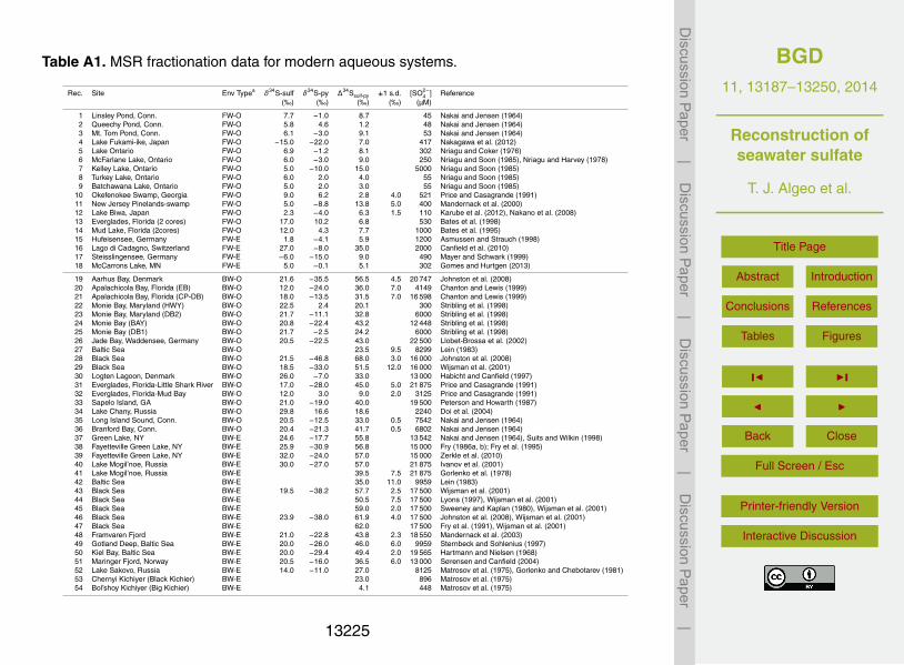
BGD11, 13187–13250, 2014


T. J. Algeo et al.

Title Page



Tables Figures

J I

J I

Back Close

Full Screen / Esc



Discussion

Paper

|D

iscussionP

aper|

Discussion

Paper

|D

iscussionP

aper|

Table A1. MSR fractionation data for modern aqueous systems.

Rec. Site Env Typea δ34S-sulf δ34S-py ∆34Ssulf-py ±1 s.d. [SO2−4 ] Reference

(‰) (‰) (‰) (‰) (µM)

1 Linsley Pond, Conn. FW-O 7.7 −1.0 8.7 45 Nakai and Jensen (1964)2 Queechy Pond, Conn. FW-O 5.8 4.6 1.2 48 Nakai and Jensen (1964)3 Mt. Tom Pond, Conn. FW-O 6.1 −3.0 9.1 53 Nakai and Jensen (1964)4 Lake Fukami-ike, Japan FW-O −15.0 −22.0 7.0 417 Nakagawa et al. (2012)5 Lake Ontario FW-O 6.9 −1.2 8.1 302 Nriagu and Coker (1976)6 McFarlane Lake, Ontario FW-O 6.0 −3.0 9.0 250 Nriagu and Soon (1985), Nriagu and Harvey (1978)7 Kelley Lake, Ontario FW-O 5.0 −10.0 15.0 5000 Nriagu and Soon (1985)8 Turkey Lake, Ontario FW-O 6.0 2.0 4.0 55 Nriagu and Soon (1985)9 Batchawana Lake, Ontario FW-O 5.0 2.0 3.0 55 Nriagu and Soon (1985)

10 Okefenokee Swamp, Georgia FW-O 9.0 6.2 2.8 4.0 521 Price and Casagrande (1991)11 New Jersey Pinelands-swamp FW-O 5.0 −8.8 13.8 5.0 400 Mandernack et al. (2000)12 Lake Biwa, Japan FW-O 2.3 −4.0 6.3 1.5 110 Karube et al. (2012), Nakano et al. (2008)13 Everglades, Florida (2 cores) FW-O 17.0 10.2 6.8 530 Bates et al. (1998)14 Mud Lake, Florida (2cores) FW-O 12.0 4.3 7.7 1000 Bates et al. (1995)15 Hufeisensee, Germany FW-E 1.8 −4.1 5.9 1200 Asmussen and Strauch (1998)16 Lago di Cadagno, Switzerland FW-E 27.0 −8.0 35.0 2000 Canfield et al. (2010)17 Steisslingensee, Germany FW-E −6.0 −15.0 9.0 490 Mayer and Schwark (1999)18 McCarrons Lake, MN FW-E 5.0 −0.1 5.1 302 Gomes and Hurtgen (2013)

19 Aarhus Bay, Denmark BW-O 21.6 −35.5 56.5 4.5 20 747 Johnston et al. (2008)20 Apalachicola Bay, Florida (EB) BW-O 12.0 −24.0 36.0 7.0 4149 Chanton and Lewis (1999)21 Apalachicola Bay, Florida (CP-DB) BW-O 18.0 −13.5 31.5 7.0 16 598 Chanton and Lewis (1999)22 Monie Bay, Maryland (HWY) BW-O 22.5 2.4 20.1 300 Stribling et al. (1998)23 Monie Bay, Maryland (DB2) BW-O 21.7 −11.1 32.8 6000 Stribling et al. (1998)24 Monie Bay (BAY) BW-O 20.8 −22.4 43.2 12 448 Stribling et al. (1998)25 Monie Bay (DB1) BW-O 21.7 −2.5 24.2 6000 Stribling et al. (1998)26 Jade Bay, Waddensee, Germany BW-O 20.5 −22.5 43.0 22 500 Llobet-Brossa et al. (2002)27 Baltic Sea BW-O 23.5 9.5 8299 Lein (1983)28 Black Sea BW-O 21.5 −46.8 68.0 3.0 16 000 Johnston et al. (2008)29 Black Sea BW-O 18.5 −33.0 51.5 12.0 16 000 Wijsman et al. (2001)30 Logten Lagoon, Denmark BW-O 26.0 −7.0 33.0 13 000 Habicht and Canfield (1997)31 Everglades, Florida-Little Shark River BW-O 17.0 −28.0 45.0 5.0 21 875 Price and Casagrande (1991)32 Everglades, Florida-Mud Bay BW-O 12.0 3.0 9.0 2.0 3125 Price and Casagrande (1991)33 Sapelo Island, GA BW-O 21.0 −19.0 40.0 19 500 Peterson and Howarth (1987)34 Lake Chany, Russia BW-O 29.8 16.6 18.6 2240 Doi et al. (2004)35 Long Island Sound, Conn. BW-O 20.5 −12.5 33.0 0.5 7542 Nakai and Jensen (1964)36 Branford Bay, Conn. BW-O 20.4 −21.3 41.7 0.5 6802 Nakai and Jensen (1964)37 Green Lake, NY BW-E 24.6 −17.7 55.8 13 542 Nakai and Jensen (1964), Suits and Wilkin (1998)38 Fayetteville Green Lake, NY BW-E 25.9 −30.9 56.8 15 000 Fry (1986a, b); Fry et al. (1995)39 Fayetteville Green Lake, NY BW-E 32.0 −24.0 57.0 15 000 Zerkle et al. (2010)40 Lake Mogil’noe, Russia BW-E 30.0 −27.0 57.0 21 875 Ivanov et al. (2001)41 Lake Mogil’noe, Russia BW-E 39.5 7.5 21 875 Gorlenko et al. (1978)42 Baltic Sea BW-E 35.0 11.0 9959 Lein (1983)43 Black Sea BW-E 19.5 −38.2 57.7 2.5 17 500 Wijsman et al. (2001)44 Black Sea BW-E 50.5 7.5 17 500 Lyons (1997), Wijsman et al. (2001)45 Black Sea BW-E 59.0 2.0 17 500 Sweeney and Kaplan (1980), Wijsman et al. (2001)46 Black Sea BW-E 23.9 −38.0 61.9 4.0 17 500 Johnston et al. (2008), Wijsman et al. (2001)47 Black Sea BW-E 62.0 17 500 Fry et al. (1991), Wijsman et al. (2001)48 Framvaren Fjord BW-E 21.0 −22.8 43.8 2.3 18 550 Mandernack et al. (2003)49 Gotland Deep, Baltic Sea BW-E 20.0 −26.0 46.0 6.0 9959 Sternbeck and Sohlenius (1997)50 Kiel Bay, Baltic Sea BW-E 20.0 −29.4 49.4 2.0 19 565 Hartmann and Nielsen (1968)51 Maringer Fjord, Norway BW-E 20.5 −16.0 36.5 6.0 13 000 Sørensen and Canfield (2004)52 Lake Sakovo, Russia BW-E 14.0 −11.0 27.0 8125 Matrosov et al. (1975), Gorlenko and Chebotarev (1981)53 Chernyi Kichiyer (Black Kichier) BW-E 23.0 896 Matrosov et al. (1975)54 Bol’shoy Kichiyer (Big Kichier) BW-E 4.1 448 Matrosov et al. (1975)

13225





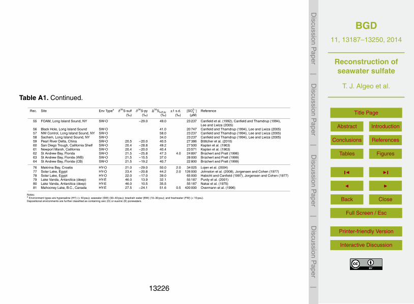
BGD11, 13187–13250, 2014


T. J. Algeo et al.

Title Page



Tables Figures

J I

J I

Back Close

Full Screen / Esc



Discussion

Paper

|D

iscussionP

aper|

Discussion

Paper

|D

iscussionP

aper|

Table A1. Continued.

Rec. Site Env Typea δ34S-sulf δ34S-py ∆34Ssulf-py ±1 s.d. [SO2−4 ] Reference

(‰) (‰) (‰) (‰) (µM)

55 FOAM, Long Island Sound, NY SW-O −29.0 49.0 23 237 Canfield et al. (1992), Canfield and Thamdrup (1994),Lee and Lwiza (2005)

56 Black Hole, Long Island Sound SW-O 41.0 20 747 Canfield and Thamdrup (1994), Lee and Lwiza (2005)57 NW Control, Long Island Sound, NY SW-O 58.0 23 237 Canfield and Thamdrup (1994), Lee and Lwiza (2005)58 Sachem, Long Island Sound, NY SW-O 34.0 23 237 Canfield and Thamdrup (1994), Lee and Lwiza (2005)59 Pearl River Delta, China SW-O 20.5 −20.0 40.5 27 386 Böttcher et al. (2010)60 San Diego Trough, California Shelf SW-O 20.4 −28.8 49.2 27 500 Kaplan et al. (1963)61 Newport Marsh, California SW-O 20.4 −20.0 40.4 23 571 Kaplan et al. (1963)62 St Andrew Bay, Florida SW-O 21.5 −25.8 47.3 4.0 24 897 Brüchert and Pratt (1996)63 St Andrew Bay, Florida (WB) SW-O 21.5 −15.5 37.0 28 000 Brüchert and Pratt (1999)64 St Andrew Bay, Florida (CB) SW-O 21.5 −19.2 40.7 22 800 Brüchert and Pratt (1999)

76 Makirina Bay, Croatia HY-O 21.0 −29.0 50.0 2.0 34 025 Lojen et al. (2004)77 Solar Lake, Egypt HY-O 23.4 −20.8 44.2 2.0 126 000 Johnston et al. (2008), Jorgensen and Cohen (1977)78 Solar Lake, Egypt HY-O 22.0 −17.0 39.0 65 000 Habicht and Canfield (1997), Jorgensen and Cohen (1977)79 Lake Vanda, Antarctica (deep) HY-E 46.0 13.9 32.1 55 187 Purdy et al. (2001)80 Lake Vanda, Antarctica (deep) HY-E 46.0 10.5 35.5 55 187 Nakai et al. (1975)81 Mahooney Lake, B.C., Canada HY-E 27.5 −24.1 51.6 0.5 420 000 Overmann et al. (1996)

Notes:a Environment types are hypersaline (HY) (> 40 psu); seawater (SW) (30–40 psu); brackish water (BW) (10–30 psu); and freshwater (FW) (< 10 psu).Depositional environments are further classified as containing oxic (O) or euxinic (E) porewaters.

13226





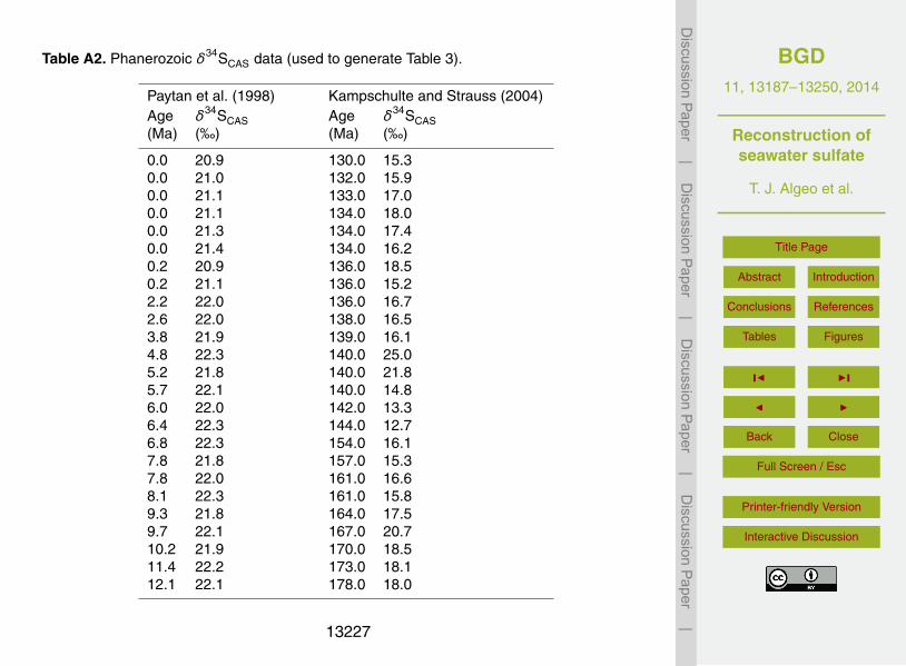
BGD11, 13187–13250, 2014


T. J. Algeo et al.

Title Page



Tables Figures

J I

J I

Back Close

Full Screen / Esc



Discussion

Paper

|D

iscussionP

aper|

Discussion

Paper

|D

iscussionP

aper|

Table A2. Phanerozoic δ34SCAS data (used to generate Table 3).

Paytan et al. (1998) Kampschulte and Strauss (2004)Age δ34SCAS Age δ34SCAS(Ma) (‰) (Ma) (‰)

0.0 20.9 130.0 15.30.0 21.0 132.0 15.90.0 21.1 133.0 17.00.0 21.1 134.0 18.00.0 21.3 134.0 17.40.0 21.4 134.0 16.20.2 20.9 136.0 18.50.2 21.1 136.0 15.22.2 22.0 136.0 16.72.6 22.0 138.0 16.53.8 21.9 139.0 16.14.8 22.3 140.0 25.05.2 21.8 140.0 21.85.7 22.1 140.0 14.86.0 22.0 142.0 13.36.4 22.3 144.0 12.76.8 22.3 154.0 16.17.8 21.8 157.0 15.37.8 22.0 161.0 16.68.1 22.3 161.0 15.89.3 21.8 164.0 17.59.7 22.1 167.0 20.710.2 21.9 170.0 18.511.4 22.2 173.0 18.112.1 22.1 178.0 18.0

13227





BGD11, 13187–13250, 2014


T. J. Algeo et al.

Title Page



Tables Figures

J I

J I

Back Close

Full Screen / Esc



Discussion

Paper

|D

iscussionP

aper|

Discussion

Paper

|D

iscussionP

aper|



12.6 21.9 184.0 23.612.6 22.0 187.0 17.412.7 22.0 197.0 14.312.7 22.7 208.0 24.412.8 22.2 210.0 18.512.9 22.7 211.0 18.013.4 22.1 214.0 19.013.7 22.0 216.0 17.414.2 21.7 221.0 19.215.1 22.0 225.0 18.515.1 22.1 237.0 17.515.7 22.4 240.0 20.116.3 21.8 242.0 26.416.3 22.0 245.0 16.717.2 22.1 245.0 15.718.1 21.9 246.0 24.519.0 21.8 253.0 10.920.0 21.6 264.0 12.521.0 22.0 289.0 12.522.2 22.0 295.0 11.823.5 21.9 297.0 12.324.1 21.9 298.0 11.025.6 21.7 304.0 12.926.4 21.4 305.0 13.326.4 21.8 306.0 13.8

13228





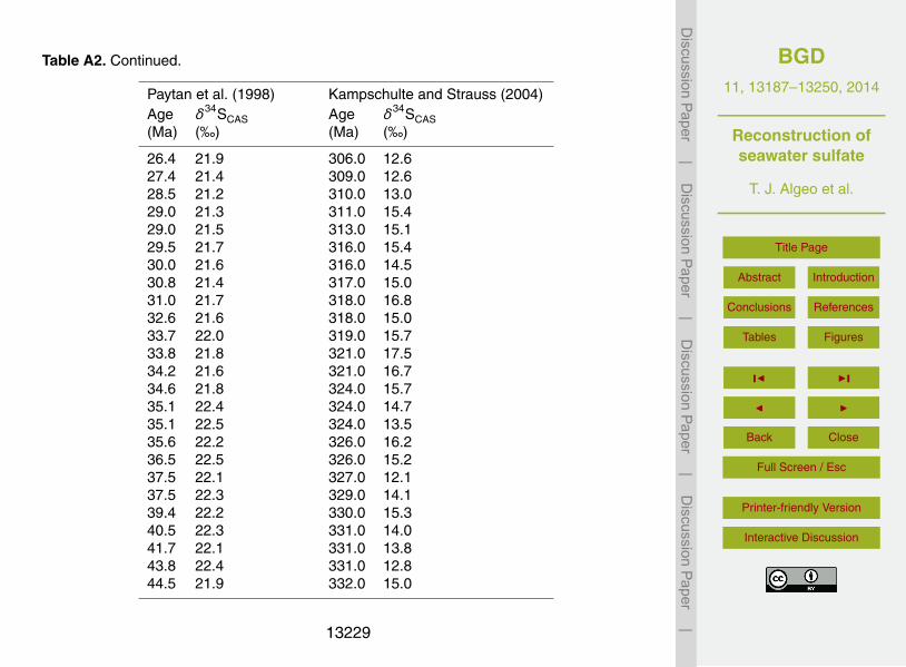
BGD11, 13187–13250, 2014


T. J. Algeo et al.

Title Page



Tables Figures

J I

J I

Back Close

Full Screen / Esc



Discussion

Paper

|D

iscussionP

aper|

Discussion

Paper

|D

iscussionP

aper|



26.4 21.9 306.0 12.627.4 21.4 309.0 12.628.5 21.2 310.0 13.029.0 21.3 311.0 15.429.0 21.5 313.0 15.129.5 21.7 316.0 15.430.0 21.6 316.0 14.530.8 21.4 317.0 15.031.0 21.7 318.0 16.832.6 21.6 318.0 15.033.7 22.0 319.0 15.733.8 21.8 321.0 17.534.2 21.6 321.0 16.734.6 21.8 324.0 15.735.1 22.4 324.0 14.735.1 22.5 324.0 13.535.6 22.2 326.0 16.236.5 22.5 326.0 15.237.5 22.1 327.0 12.137.5 22.3 329.0 14.139.4 22.2 330.0 15.340.5 22.3 331.0 14.041.7 22.1 331.0 13.843.8 22.4 331.0 12.844.5 21.9 332.0 15.0

13229





BGD11, 13187–13250, 2014


T. J. Algeo et al.

Title Page



Tables Figures

J I

J I

Back Close

Full Screen / Esc



Discussion

Paper

|D

iscussionP

aper|

Discussion

Paper

|D

iscussionP

aper|



44.5 22.0 334.0 14.546.0 21.6 334.0 13.746.0 21.5 335.0 12.948.2 20.3 336.0 15.649.7 19.1 337.0 14.549.9 19.3 338.0 12.850.2 19.1 339.0 13.451.2 18.7 343.0 14.651.6 18.0 343.0 13.751.9 18.1 345.0 15.953.6 17.8 346.0 21.255.5 17.4 349.0 17.756.4 17.7 351.0 18.557.0 17.5 353.0 17.657.6 18.2 355.0 23.357.6 18.3 355.0 21.357.9 17.9 360.0 20.657.9 18.0 360.0 19.759.2 18.1 380.0 22.760.7 18.6 380.0 22.060.9 19.0 383.0 16.461.8 19.1 386.0 17.363.9 18.8 391.0 23.365.2 19.0 403.0 24.565.2 18.9 406.0 28.5

13230





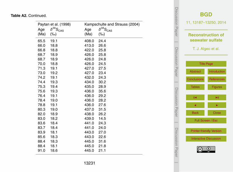
BGD11, 13187–13250, 2014


T. J. Algeo et al.

Title Page



Tables Figures

J I

J I

Back Close

Full Screen / Esc



Discussion

Paper

|D

iscussionP

aper|

Discussion

Paper

|D

iscussionP

aper|



65.5 19.1 408.0 24.466.0 18.8 413.0 26.666.8 18.8 422.0 25.868.7 18.9 426.0 25.868.7 18.9 426.0 24.870.0 18.8 426.0 24.571.3 19.1 427.0 27.573.0 19.2 427.0 23.474.2 19.1 432.0 24.374.4 19.3 434.0 30.275.3 19.4 435.0 28.975.6 19.3 436.0 35.676.4 19.1 436.0 29.278.4 19.0 436.0 28.278.8 19.1 436.0 27.680.3 19.0 437.0 31.582.0 18.9 438.0 26.283.0 18.2 439.0 14.583.6 18.4 441.0 24.383.7 18.4 441.0 24.083.9 18.1 443.0 27.085.6 18.3 443.0 22.688.4 18.3 445.0 31.688.4 18.1 445.0 21.891.0 18.6 445.0 21.1

13231





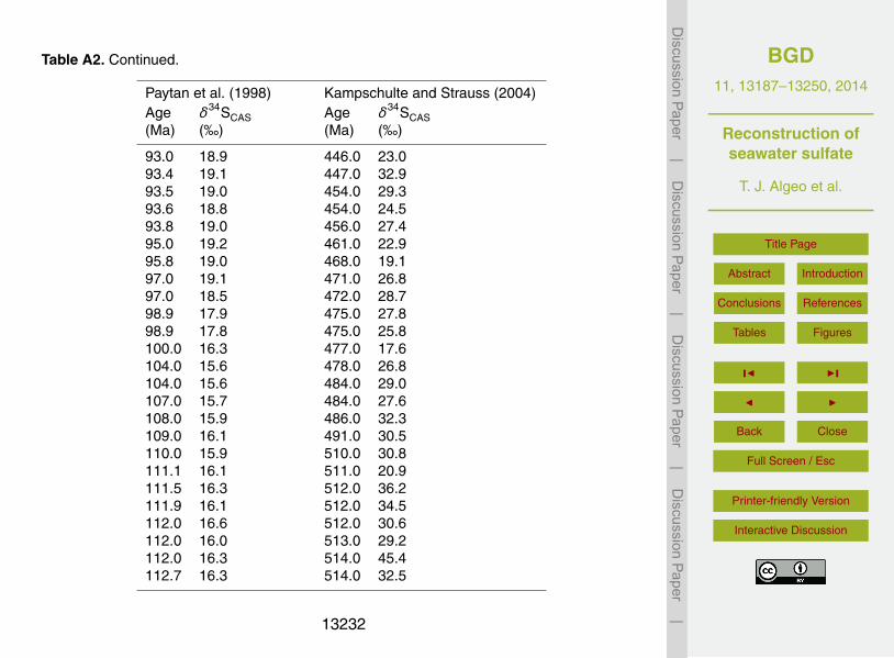
BGD11, 13187–13250, 2014


T. J. Algeo et al.

Title Page



Tables Figures

J I

J I

Back Close

Full Screen / Esc



Discussion

Paper

|D

iscussionP

aper|

Discussion

Paper

|D

iscussionP

aper|



93.0 18.9 446.0 23.093.4 19.1 447.0 32.993.5 19.0 454.0 29.393.6 18.8 454.0 24.593.8 19.0 456.0 27.495.0 19.2 461.0 22.995.8 19.0 468.0 19.197.0 19.1 471.0 26.897.0 18.5 472.0 28.798.9 17.9 475.0 27.898.9 17.8 475.0 25.8100.0 16.3 477.0 17.6104.0 15.6 478.0 26.8104.0 15.6 484.0 29.0107.0 15.7 484.0 27.6108.0 15.9 486.0 32.3109.0 16.1 491.0 30.5110.0 15.9 510.0 30.8111.1 16.1 511.0 20.9111.5 16.3 512.0 36.2111.9 16.1 512.0 34.5112.0 16.6 512.0 30.6112.0 16.0 513.0 29.2112.0 16.3 514.0 45.4112.7 16.3 514.0 32.5

13232





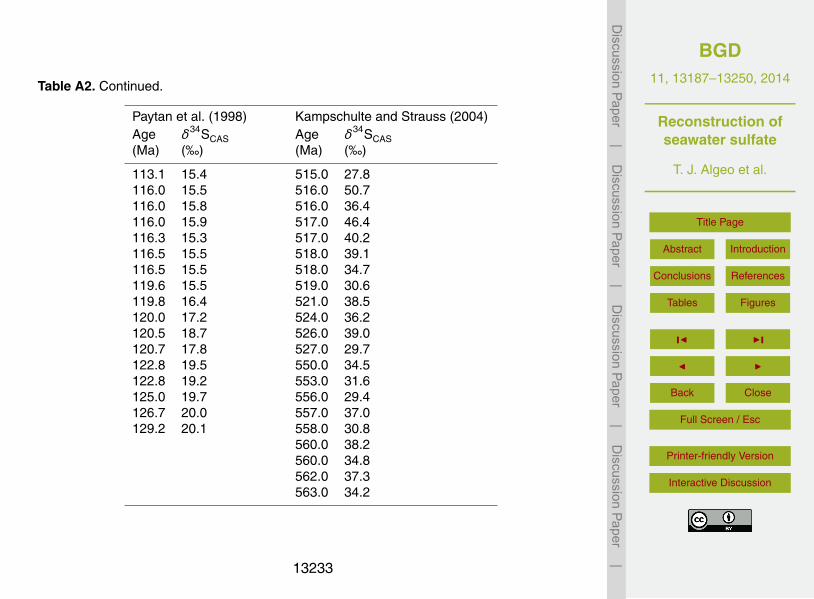
BGD11, 13187–13250, 2014


T. J. Algeo et al.

Title Page



Tables Figures

J I

J I

Back Close

Full Screen / Esc



Discussion

Paper

|D

iscussionP

aper|

Discussion

Paper

|D

iscussionP

aper|



113.1 15.4 515.0 27.8116.0 15.5 516.0 50.7116.0 15.8 516.0 36.4116.0 15.9 517.0 46.4116.3 15.3 517.0 40.2116.5 15.5 518.0 39.1116.5 15.5 518.0 34.7119.6 15.5 519.0 30.6119.8 16.4 521.0 38.5120.0 17.2 524.0 36.2120.5 18.7 526.0 39.0120.7 17.8 527.0 29.7122.8 19.5 550.0 34.5122.8 19.2 553.0 31.6125.0 19.7 556.0 29.4126.7 20.0 557.0 37.0129.2 20.1 558.0 30.8

560.0 38.2560.0 34.8562.0 37.3563.0 34.2

13233





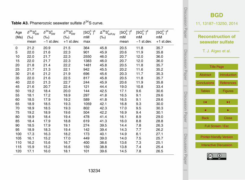
BGD11, 13187–13250, 2014


T. J. Algeo et al.

Title Page



Tables Figures

J I

J I

Back Close

Full Screen / Esc



Discussion

Paper

|D

iscussionP

aper|

Discussion

Paper

|D

iscussionP

aper|

Table A3. Phanerozoic seawater sulfate δ34S curve.

Age δ34SaSW δ34Sa

SW δ34SaSW [SO2−

4 ]b ∆34Scsulf-py [SO2−

4 ]d [SO2−4 ]d [SO2−

4 ]d

(Ma) (‰) (‰) (‰) mM (‰) mM mM mMmean −1 st.dev. +1 st.dev. max mean −1 st.dev. +1 st.dev.

0 21.2 20.9 21.5 364 45.8 20.5 11.8 35.75 22.0 21.6 22.3 901 45.9 20.6 11.9 35.810 22.0 21.7 22.3 2550 46.0 20.7 12.0 36.015 22.0 21.7 22.3 1383 46.0 20.7 12.0 36.020 21.8 21.4 22.2 1481 45.8 20.5 11.8 35.725 21.7 21.3 22.1 942 45.5 20.2 11.6 35.230 21.6 21.2 21.9 696 45.6 20.3 11.7 35.335 22.0 21.6 22.5 817 45.8 20.5 11.8 35.740 22.0 21.3 22.7 244 45.9 20.6 11.9 35.845 21.6 20.7 22.4 121 44.4 19.0 10.8 33.450 19.2 18.4 20.0 144 42.5 17.1 9.6 30.655 18.1 17.2 18.9 297 41.8 16.5 9.1 29.660 18.5 17.9 19.2 589 41.8 16.5 9.1 29.665 18.9 18.5 19.3 1059 42.1 16.8 9.3 30.070 18.9 18.5 19.3 802 42.3 17.0 9.5 30.375 19.2 18.9 19.6 504 42.2 16.9 9.4 30.180 18.9 18.4 19.4 478 41.4 16.1 8.9 29.085 18.4 17.9 18.8 619 41.3 16.0 8.8 28.890 18.5 17.9 19.1 274 39.5 14.4 7.8 26.395 18.9 18.3 19.4 142 39.4 14.3 7.7 26.2100 17.3 16.3 18.2 173 40.1 14.9 8.1 27.1105 16.1 15.2 17.0 449 39.0 14.0 7.5 25.7110 16.2 15.6 16.7 400 38.6 13.6 7.3 25.1115 15.9 15.2 16.6 150 38.8 13.8 7.4 25.4120 17.1 16.0 18.1 101 39.6 14.5 7.8 26.5

13234





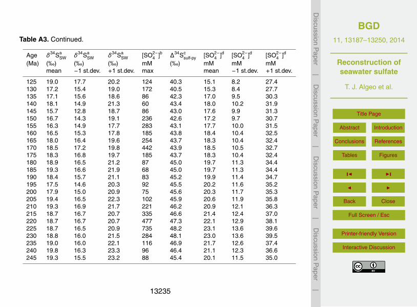
BGD11, 13187–13250, 2014


T. J. Algeo et al.

Title Page



Tables Figures

J I

J I

Back Close

Full Screen / Esc



Discussion

Paper

|D

iscussionP

aper|

Discussion

Paper

|D

iscussionP

aper|


Age δ34SaSW δ34Sa

SW δ34SaSW [SO2−


4 ]d [SO2−4 ]d [SO2−

4 ]d


125 19.0 17.7 20.2 124 40.3 15.1 8.2 27.4130 17.2 15.4 19.0 172 40.5 15.3 8.4 27.7135 17.1 15.6 18.6 86 42.3 17.0 9.5 30.3140 18.1 14.9 21.3 60 43.4 18.0 10.2 31.9145 15.7 12.8 18.7 86 43.0 17.6 9.9 31.3150 16.7 14.3 19.1 236 42.6 17.2 9.7 30.7155 16.3 14.9 17.7 283 43.1 17.7 10.0 31.5160 16.5 15.3 17.8 185 43.8 18.4 10.4 32.5165 18.0 16.4 19.6 254 43.7 18.3 10.4 32.4170 18.5 17.2 19.8 442 43.9 18.5 10.5 32.7175 18.3 16.8 19.7 185 43.7 18.3 10.4 32.4180 18.9 16.5 21.2 87 45.0 19.7 11.3 34.4185 19.3 16.6 21.9 68 45.0 19.7 11.3 34.4190 18.4 15.7 21.1 83 45.2 19.9 11.4 34.7195 17.5 14.6 20.3 92 45.5 20.2 11.6 35.2200 17.9 15.0 20.9 75 45.6 20.3 11.7 35.3205 19.4 16.5 22.3 102 45.9 20.6 11.9 35.8210 19.3 16.9 21.7 221 46.2 20.9 12.1 36.3215 18.7 16.7 20.7 335 46.6 21.4 12.4 37.0220 18.7 16.7 20.7 477 47.3 22.1 12.9 38.1225 18.7 16.5 20.9 735 48.2 23.1 13.6 39.6230 18.8 16.0 21.5 284 48.1 23.0 13.6 39.5235 19.0 16.0 22.1 116 46.9 21.7 12.6 37.4240 19.8 16.3 23.3 96 46.4 21.1 12.3 36.6245 19.3 15.5 23.2 88 45.4 20.1 11.5 35.0

13235





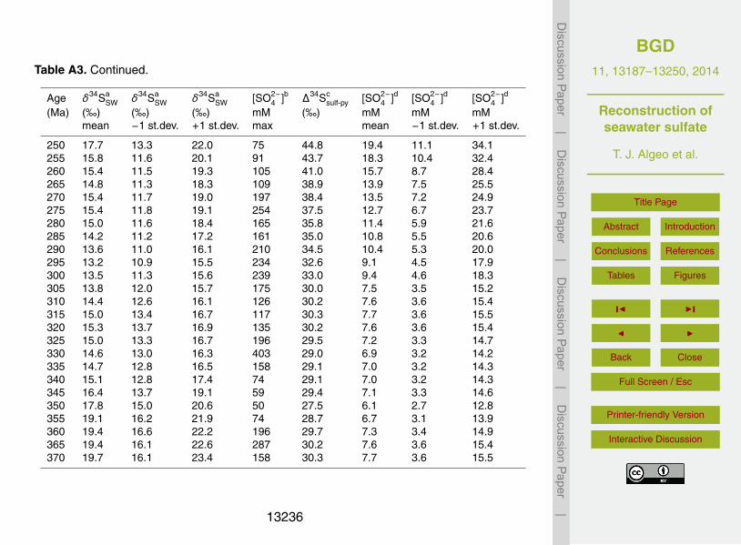
BGD11, 13187–13250, 2014


T. J. Algeo et al.

Title Page



Tables Figures

J I

J I

Back Close

Full Screen / Esc



Discussion

Paper

|D

iscussionP

aper|

Discussion

Paper

|D

iscussionP

aper|


Age δ34SaSW δ34Sa

SW δ34SaSW [SO2−


4 ]d [SO2−4 ]d [SO2−

4 ]d


250 17.7 13.3 22.0 75 44.8 19.4 11.1 34.1255 15.8 11.6 20.1 91 43.7 18.3 10.4 32.4260 15.4 11.5 19.3 105 41.0 15.7 8.7 28.4265 14.8 11.3 18.3 109 38.9 13.9 7.5 25.5270 15.4 11.7 19.0 197 38.4 13.5 7.2 24.9275 15.4 11.8 19.1 254 37.5 12.7 6.7 23.7280 15.0 11.6 18.4 165 35.8 11.4 5.9 21.6285 14.2 11.2 17.2 161 35.0 10.8 5.5 20.6290 13.6 11.0 16.1 210 34.5 10.4 5.3 20.0295 13.2 10.9 15.5 234 32.6 9.1 4.5 17.9300 13.5 11.3 15.6 239 33.0 9.4 4.6 18.3305 13.8 12.0 15.7 175 30.0 7.5 3.5 15.2310 14.4 12.6 16.1 126 30.2 7.6 3.6 15.4315 15.0 13.4 16.7 117 30.3 7.7 3.6 15.5320 15.3 13.7 16.9 135 30.2 7.6 3.6 15.4325 15.0 13.3 16.7 196 29.5 7.2 3.3 14.7330 14.6 13.0 16.3 403 29.0 6.9 3.2 14.2335 14.7 12.8 16.5 158 29.1 7.0 3.2 14.3340 15.1 12.8 17.4 74 29.1 7.0 3.2 14.3345 16.4 13.7 19.1 59 29.4 7.1 3.3 14.6350 17.8 15.0 20.6 50 27.5 6.1 2.7 12.8355 19.1 16.2 21.9 74 28.7 6.7 3.1 13.9360 19.4 16.6 22.2 196 29.7 7.3 3.4 14.9365 19.4 16.1 22.6 287 30.2 7.6 3.6 15.4370 19.7 16.1 23.4 158 30.3 7.7 3.6 15.5

13236





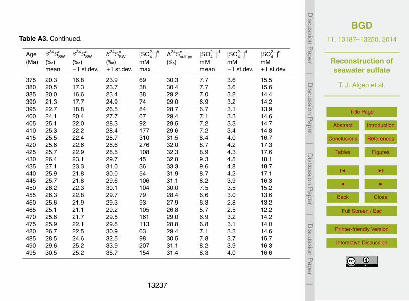
BGD11, 13187–13250, 2014


T. J. Algeo et al.

Title Page



Tables Figures

J I

J I

Back Close

Full Screen / Esc



Discussion

Paper

|D

iscussionP

aper|

Discussion

Paper

|D

iscussionP

aper|


Age δ34SaSW δ34Sa

SW δ34SaSW [SO2−


4 ]d [SO2−4 ]d [SO2−

4 ]d


375 20.3 16.8 23.9 69 30.3 7.7 3.6 15.5380 20.5 17.3 23.7 38 30.4 7.7 3.6 15.6385 20.0 16.6 23.4 38 29.2 7.0 3.2 14.4390 21.3 17.7 24.9 74 29.0 6.9 3.2 14.2395 22.7 18.8 26.5 84 28.7 6.7 3.1 13.9400 24.1 20.4 27.7 67 29.4 7.1 3.3 14.6405 25.1 22.0 28.3 92 29.5 7.2 3.3 14.7410 25.3 22.2 28.4 177 29.6 7.2 3.4 14.8415 25.5 22.4 28.7 310 31.5 8.4 4.0 16.7420 25.6 22.6 28.6 276 32.0 8.7 4.2 17.3425 25.7 22.9 28.5 108 32.3 8.9 4.3 17.6430 26.4 23.1 29.7 45 32.8 9.3 4.5 18.1435 27.1 23.3 31.0 36 33.3 9.6 4.8 18.7440 25.9 21.8 30.0 54 31.9 8.7 4.2 17.1445 25.7 21.8 29.6 106 31.1 8.2 3.9 16.3450 26.2 22.3 30.1 104 30.0 7.5 3.5 15.2455 26.3 22.8 29.7 79 28.4 6.6 3.0 13.6460 25.6 21.9 29.3 93 27.9 6.3 2.8 13.2465 25.1 21.1 29.2 105 26.8 5.7 2.5 12.2470 25.6 21.7 29.5 161 29.0 6.9 3.2 14.2475 25.9 22.1 29.8 113 28.8 6.8 3.1 14.0480 26.7 22.5 30.9 63 29.4 7.1 3.3 14.6485 28.5 24.6 32.5 98 30.5 7.8 3.7 15.7490 29.6 25.2 33.9 207 31.1 8.2 3.9 16.3495 30.5 25.2 35.7 154 31.4 8.3 4.0 16.6

13237





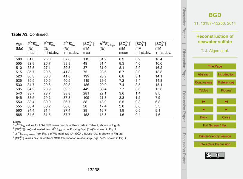
BGD11, 13187–13250, 2014


T. J. Algeo et al.

Title Page



Tables Figures

J I

J I

Back Close

Full Screen / Esc



Discussion

Paper

|D

iscussionP

aper|

Discussion

Paper

|D

iscussionP

aper|


Age δ34SaSW δ34Sa

SW δ34SaSW [SO2−


4 ]d [SO2−4 ]d [SO2−

4 ]d


500 31.8 25.8 37.8 113 31.2 8.2 3.9 16.4505 32.8 26.7 38.8 49 31.4 8.3 4.0 16.6510 33.5 27.4 39.5 37 31.0 8.1 3.9 16.2515 35.7 29.6 41.8 75 28.6 6.7 3.0 13.8520 36.3 30.8 41.8 199 28.9 6.8 3.1 14.1525 35.5 30.5 40.5 115 29.6 7.2 3.4 14.8530 34.7 29.6 39.8 186 29.9 7.4 3.5 15.1535 34.2 28.9 39.5 449 30.4 7.7 3.6 15.6540 33.7 28.7 38.8 281 22.1 3.6 1.4 8.5545 33.5 29.2 37.8 109 21.3 3.3 1.2 7.9550 33.4 30.0 36.7 38 18.9 2.5 0.8 6.3555 33.4 30.2 36.6 28 17.4 2.0 0.6 5.5560 34.4 31.4 37.4 39 16.7 1.9 0.5 5.1565 34.6 31.5 37.7 153 15.8 1.6 0.4 4.6

Notes:a δ34SSW values for LOWESS curve calculated from data in Table 2; shown in Fig. 3a.b [SO2−

4 ](max) calculated from δ34SSW in col B using Eqs. (1)–(3); shown in Fig. 4.c ∆34Ssulf-py values from Fig. 3 of Wu et al. (2010), GCA 74:2053–2071; shown in Fig. 3c.d [SO2−

4 ] values calculated from MSR fractionation relationship (Eqs. 5–7); shown in Fig. 4.

13238





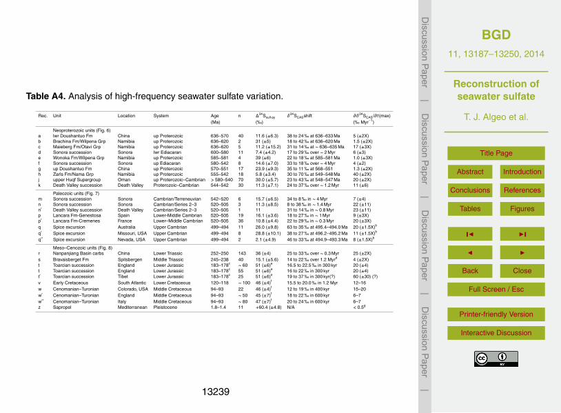
BGD11, 13187–13250, 2014


T. J. Algeo et al.

Title Page



Tables Figures

J I

J I

Back Close

Full Screen / Esc



Discussion

Paper

|D

iscussionP

aper|

Discussion

Paper

|D

iscussionP

aper|

Table A4. Analysis of high-frequency seawater sulfate variation.

Rec. Unit Location System Age n ∆34Ssulf-py δ34SCASshift ∂δ34SCAS/∂t(max)(Ma) (‰) (‰ Myr−1)

Neoproterozoic units (Fig. 6)a lwr Doushantuo Fm China up Proterozoic 636–570 40 11.6 (±6.3) 38 to 24 ‰ at 636–633 Ma 5 (±2X)b Brachina Fm/Wilpena Grp Namibia up Proterozoic 636–620 2 31 (±5) 18 to 42 ‰ at 636–620 Ma 1.5 (±2X)c Maieberg Fm/Otavi Grp Namibia up Proterozoic 636–620 5 11.2 (±15.2) 31 to 14 ‰ at ∼ 636–635 Ma 17 (±3X)d Sonora succession Sonora lwr Ediacaran 600–580 11 7.4 (±4.2) 17 to 29 ‰ over ∼ 2 Myr 6 (±3)e Wonoka Fm/Wilpena Grp Namibia up Proterozoic 585–581 4 39 (±6) 22 to 18 ‰ at 585–581 Ma 1.0 (±3X)f Sonora succession Sonora up Ediacaran 580–542 8 14.6 (±7.0) 33 to 18 ‰ over ∼ 4 Myr 4 (±2)g up Doushantuo Fm China up Proterozoic 570–551 17 23.9 (±9.3) 35 to 11 ‰ at 568–551 1.3 (±2X)h Zarls Fm/Nama Grp Namibia up Proterozoic 555–542 18 5.8 (±3.4) 30 to 70 ‰ at 549–548 Ma 40 (±2X)j upper Huqf Supergroup Oman up Proterozoic–Cambrian > 580–540 70 30.0 (±5.7) 23 to 43 ‰ at 548–547 Ma 20 (±2X)k Death Valley succession Death Valley Proterozoic–Cambrian 544–542 30 11.3 (±7.1) 24 to 37 ‰ over ∼ 1.2 Myr 11 (±6)

Paleozoic units (Fig. 7)m Sonora succession Sonora Cambrian/Terreneuvian 542–520 6 15.7 (±6.5) 34 to 8 ‰ in ∼ 4 Myr 7 (±4)n Sonora succession Sonora Cambrian/Series 2–3 520–505 3 11.3 (±8.5) 8 to 38 ‰ in ∼ 1.4 Myr 22 (±11)n′ Death Valley succession Death Valley Cambrian/Series 2–3 520–505 1 11 31 to 14 ‰ in ∼ 0.8 Myr 23 (±11)p Lancara Fm-Genestosa Spain Lower-Middle Cambrian 520–505 19 16.1 (±3.6) 18 to 27 ‰ in ∼ 1 Myr 9 (±3X)p′ Lancara Fm-Cremenes France Lower–Middle Cambrian 520–505 36 10.8 (±4.4) 22 to 29 ‰ in ∼ 0.3 Myr 20 (±3X)q Spice excursion Australia Upper Cambrian 499–494 11 26.0 (±9.8) 63 to 35 ‰ at 495.4–494.0 Ma 20 (±1.5X)b

q′ Spice excursion Missouri, USA Upper Cambrian 499–494 8 28.8 (±10.1) 38 to 27 ‰ at 496.2–495.2 Ma 11 (±1.5X)b

q′′ Spice excursion Nevada, USA Upper Cambrian 499–494 2 2.1 (±4.9) 46 to 33 ‰ at 494.9–493.3 Ma 8 (±1.5X)b

Meso–Cenozoic units (Fig. 8)r Nanpanjiang Basin carbs China Lower Triassic 252–250 143 36 (±4) 25 to 33 ‰ over ∼ 0.3 Myr 25 (±2X)s Bravaisberget Fm Spitsbergen Middle Triassic 245–238 40 15.1 (±5.6) 14 to 22 ‰ over 1.2 Myrd 4 (±2X)t Toarcian succession England Lower Jurassic 183–178c ∼ 60 51 (±6)e 16.5 to 22.5 ‰ in 300 kyr 20 (±4)t Toarcian succession England Lower Jurassic 183–178c 55 51 (±6)e 16 to 22 ‰ in 300 kyr 20 (±4)t′ Toarcian succession Tibet Lower Jurassic 183–178c 25 51 (±6)e 19 to 37 ‰ in 300 kyr(?) 60 (±30) (?)v Early Cretaceous South Atlantic Lower Cretaceous 120–118 ∼ 100 46 (±4)f 15.5 to 20.0 ‰ in 1.2 Myr 12–16w Cenomanian–Turonian Colorado, USA Middle Cretaceous 94–93 22 46 (±4)f 12 to 19 ‰ in 400 kyr 15–20w′ Cenomanian–Turonian England Middle Cretaceous 94–93 ∼ 50 45 (±7)f 18 to 22 ‰ in 600 kyr 6–7w′′ Cenomanian–Turonian Italy Middle Cretaceous 94–93 ∼ 80 47 (±7)f 20 to 24 ‰ in 600 kyr 6–7z Sapropel Mediterranean Pleistocene 1.8–1.4 11 +60.4 (±4.8) N/A < 0.5g

13239





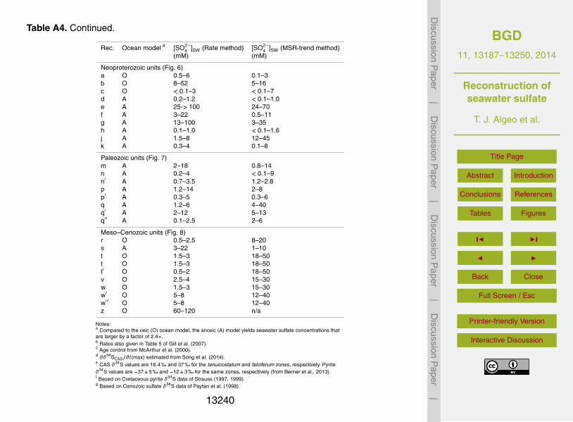
BGD11, 13187–13250, 2014


T. J. Algeo et al.

Title Page



Tables Figures

J I

J I

Back Close

Full Screen / Esc



Discussion

Paper

|D

iscussionP

aper|

Discussion

Paper

|D

iscussionP

aper|


Rec. Ocean model a [SO2−4 ]SW (Rate method) [SO2−

4 ]SW (MSR-trend method)(mM) (mM)

Neoproterozoic units (Fig. 6)a O 0.5–6 0.1–3b O 8–52 5–16c O < 0.1–3 < 0.1–7d A 0.2–1.2 < 0.1–1.0e A 25-> 100 24–70f A 3–22 0.5–11g A 13–100 3–35h A 0.1–1.0 < 0.1–1.6j A 1.5–8 12–45k A 0.3–4 0.1–8

Paleozoic units (Fig. 7)m A 2–18 0.8–14n A 0.2–4 < 0.1–9n′ A 0.7–3.5 1.2–2.8p A 1.2–14 2–8p′ A 0.3–5 0.3–6q A 1.2–6 4–40q′ A 2–12 5–13q′′ A 0.1–2.5 2–6

Meso–Cenozoic units (Fig. 8)r O 0.5–2.5 8–20s A 3–22 1–10t O 1.5–3 18–50t O 1.5–3 18–50t′ O 0.5–2 18–50v O 2.5–4 15–30w O 1.5–3 15–30w′ O 5–8 12–40w′′ O 5–8 12–40z O 60–120 n/a

Notes:a Compared to the oxic (O) ocean model, the anoxic (A) model yields seawater sulfate concentrations thatare larger by a factor of 2.4×.b Rates also given in Table 5 of Gill et al. (2007).c Age control from McArthur et al. (2000).d ∂δ34SCAS/∂t(max) estimated from Song et al. (2014).e CAS δ34S values are 16.4 ‰ and 37 ‰ for the tenuicostatum and falciferum zones, respectively. Pyriteδ34S values are −37±5 ‰ and −12±3 ‰ for the same zones, respectively (from Berner et al., 2013).f Based on Cretaceous pyrite δ34S data of Strauss (1997, 1999).g Based on Cenozoic sulfate δ34S data of Paytan et al. (1998).

13240





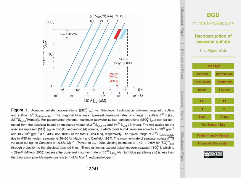
BGD11, 13187–13250, 2014


T. J. Algeo et al.

Title Page



Tables Figures

J I

J I

Back Close

Full Screen / Esc



Discussion

Paper

|D

iscussionP

aper|

Discussion

Paper

|D

iscussionP

aper|

Figure 1. Aqueous sulfate concentrations ([SO2−4 ]aq) vs. S-isotopic fractionation between cogenetic sulfate

and sulfide (∆34Ssulfate-sulfide). The diagonal blue lines represent maximum rates of change in sulfate δ34S (i.e.,∂δ34SSO4

/∂t(max)). For paleomarine systems, maximum seawater sulfate concentrations ([SO2−4 ]SW) can be esti-

mated from the abscissa based on measured values of ∆34SCAS-PY and ∂δ34SCAS/∂t(max). The two scales on theabscissa represent [SO2−

4 ]SW in oxic (O) and anoxic (A) oceans, in which pyrite burial fluxes are equal to 4×1013 g yr−1

and 10×1013 g yr−1 (i.e., 40 % and 100 % of the total S sink flux), respectively. The typical range of ∆34Ssulfate-sulfide

due to MSR in modern seawater is 30–60 ‰ (Habicht and Canfield, 1997). The maximum rate of seawater sulfate δ34Svariation during the Cenozoic is ∼0.5 ‰ Myr−1 (Paytan et al., 1998), yielding estimates of ∼ 40–110 mM for [SO2−

4 ]SW

through projection to the abscissa (dashed lines). These estimates exceed actual modern seawater [SO2−4 ], which is

∼ 29 mM (Millero, 2005) because the observed maximum rate of ∂δ34SSO4/∂t (light blue parallelogram) is less than

the theoretical possible maximum rate (∼ 1–2 ‰ Myr−1; red parallelogram).

13241





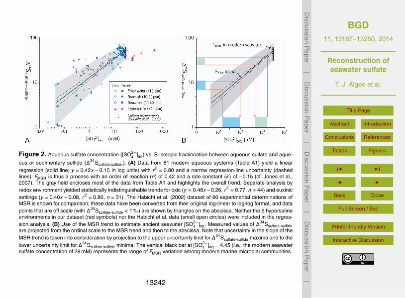
BGD11, 13187–13250, 2014


T. J. Algeo et al.

Title Page



Tables Figures

J I

J I

Back Close

Full Screen / Esc



Discussion

Paper

|D

iscussionP

aper|

Discussion

Paper

|D

iscussionP

aper|

Figure 2. Aqueous sulfate concentration ([SO2−4 ]aq) vs. S-isotopic fractionation between aqueous sulfate and aque-

ous or sedimentary sulfide (∆34Ssulfate-sulfide). (A) Data from 81 modern aqueous systems (Table A1) yield a linearregression (solid line; y = 0.42x−0.15 in log units) with r2 = 0.80 and a narrow regression-line uncertainty (dashedlines). FMSR is thus a process with an order of reaction (n) of 0.42 and a rate constant (k) of −0.15 (cf. Jones et al.,2007). The gray field encloses most of the data from Table A1 and highlights the overall trend. Separate analysis byredox environment yielded statistically indistinguishable trends for oxic (y = 0.48x−0.26, r2 = 0.77, n = 44) and euxinicsettings (y = 0.40x−0.08, r2 = 0.80, n = 31). The Habicht et al. (2002) dataset of 60 experimental determinations ofMSR is shown for comparison; these data have been converted from their original log-linear to log-log format, and datapoints that are off scale (with ∆34Ssulfate-sulfide < 1 ‰) are shown by triangles on the abscissa. Neither the 6 hypersalineenvironments in our dataset (red symbols) nor the Habicht et al. data (small open circles) were included in the regres-sion analysis. (B) Use of the MSR trend to estimate ancient seawater [SO2−

4 ]aq. Measured values of ∆34Ssulfate-sulfideare projected from the ordinal scale to the MSR trend and then to the abscissa. Note that uncertainty in the slope of theMSR trend is taken into consideration by projection to the upper uncertainty limit for ∆34Ssulfate-sulfide maxima and to thelower uncertainty limit for ∆34Ssulfate-sulfide minima. The vertical black bar at [SO2−

4 ]aq = 4.45 (i.e., the modern seawatersulfate concentration of 29 mM) represents the range of FMSR variation among modern marine microbial communities.

13242





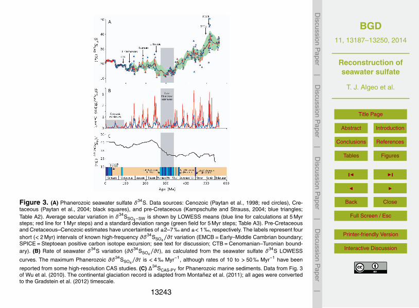
BGD11, 13187–13250, 2014


T. J. Algeo et al.

Title Page



Tables Figures

J I

J I

Back Close

Full Screen / Esc



Discussion

Paper

|D

iscussionP

aper|

Discussion

Paper

|D

iscussionP

aper|

Figure 3. (A) Phanerozoic seawater sulfate δ34S. Data sources: Cenozoic (Paytan et al., 1998; red circles), Cre-taceous (Paytan et al., 2004; black squares), and pre-Cretaceous (Kampschulte and Strauss, 2004; blue triangles;Table A2). Average secular variation in δ34SSO4−SW is shown by LOWESS means (blue line for calculations at 5 Myrsteps; red line for 1 Myr steps) and a standard deviation range (green field for 5 Myr steps; Table A3). Pre-Cretaceousand Cretaceous–Cenozoic estimates have uncertainties of ±2–7 ‰ and ±< 1 ‰, respectively. The labels represent fourshort (< 2 Myr) intervals of known high-frequency ∂δ34SSO4

/∂t variation (EMCB=Early–Middle Cambrian boundary;SPICE=Steptoean positive carbon isotope excursion; see text for discussion; CTB=Cenomanian–Turonian bound-ary). (B) Rate of seawater δ34S variation (∂δ34SSO4

/∂t), as calculated from the seawater sulfate δ34S LOWESS

curves. The maximum Phanerozoic ∂δ34SSO4/∂t is < 4 ‰ Myr−1, although rates of 10 to > 50 ‰ Myr−1 have been

reported from some high-resolution CAS studies. (C) ∆34SCAS-PY for Phanerozoic marine sediments. Data from Fig. 3of Wu et al. (2010). The continental glaciation record is adapted from Montañez et al. (2011); all ages were convertedto the Gradstein et al. (2012) timescale.

13243





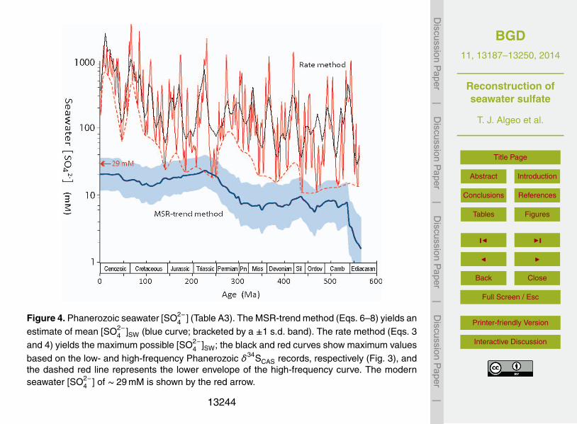
BGD11, 13187–13250, 2014


T. J. Algeo et al.

Title Page



Tables Figures

J I

J I

Back Close

Full Screen / Esc



Discussion

Paper

|D

iscussionP

aper|

Discussion

Paper

|D

iscussionP

aper|

Figure 4. Phanerozoic seawater [SO2−4 ] (Table A3). The MSR-trend method (Eqs. 6–8) yields an

estimate of mean [SO2−4 ]SW (blue curve; bracketed by a ±1 s.d. band). The rate method (Eqs. 3

and 4) yields the maximum possible [SO2−4 ]SW; the black and red curves show maximum values

based on the low- and high-frequency Phanerozoic δ34SCAS records, respectively (Fig. 3), andthe dashed red line represents the lower envelope of the high-frequency curve. The modernseawater [SO2−

4 ] of ∼ 29 mM is shown by the red arrow.

13244





BGD11, 13187–13250, 2014


T. J. Algeo et al.

Title Page



Tables Figures

J I

J I

Back Close

Full Screen / Esc



Discussion

Paper

|D

iscussionP

aper|

Discussion

Paper

|D

iscussionP

aper|

Figure 5. Comparison of Phanerozoic seawater sulfate [SO2−4 ] records. The mean trend of the

present study is shown by a heavy blue line, with the ±1σ uncertainty range shown as a blueband. Estimates are based either on fluid-inclusion studies (Horita et al., 2002; Brennan et al.,2004; Lowenstein et al., 2005) or C-S-cycle modeling (Holser et al., 1989; Berner, 2004; Gillet al., 2007; Wortmann and Chernyavsky, 2007; Wortmann and Paytan, 2012; Halevy et al.,2012). Arrows indicate unconstrained minimum or maximum values.

13245





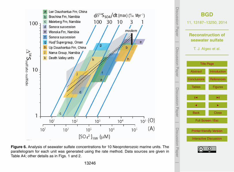
BGD11, 13187–13250, 2014


T. J. Algeo et al.

Title Page



Tables Figures

J I

J I

Back Close

Full Screen / Esc



Discussion

Paper

|D

iscussionP

aper|

Discussion

Paper

|D

iscussionP

aper|

Figure 6. Analysis of seawater sulfate concentrations for 10 Neoproterozoic marine units. Theparallelogram for each unit was generated using the rate method. Data sources are given inTable A4; other details as in Figs. 1 and 2.

13246





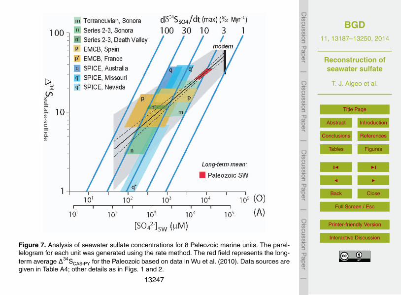
BGD11, 13187–13250, 2014


T. J. Algeo et al.

Title Page



Tables Figures

J I

J I

Back Close

Full Screen / Esc



Discussion

Paper

|D

iscussionP

aper|

Discussion

Paper

|D

iscussionP

aper|

Figure 7. Analysis of seawater sulfate concentrations for 8 Paleozoic marine units. The paral-lelogram for each unit was generated using the rate method. The red field represents the long-term average ∆34SCAS-PY for the Paleozoic based on data in Wu et al. (2010). Data sources aregiven in Table A4; other details as in Figs. 1 and 2.

13247





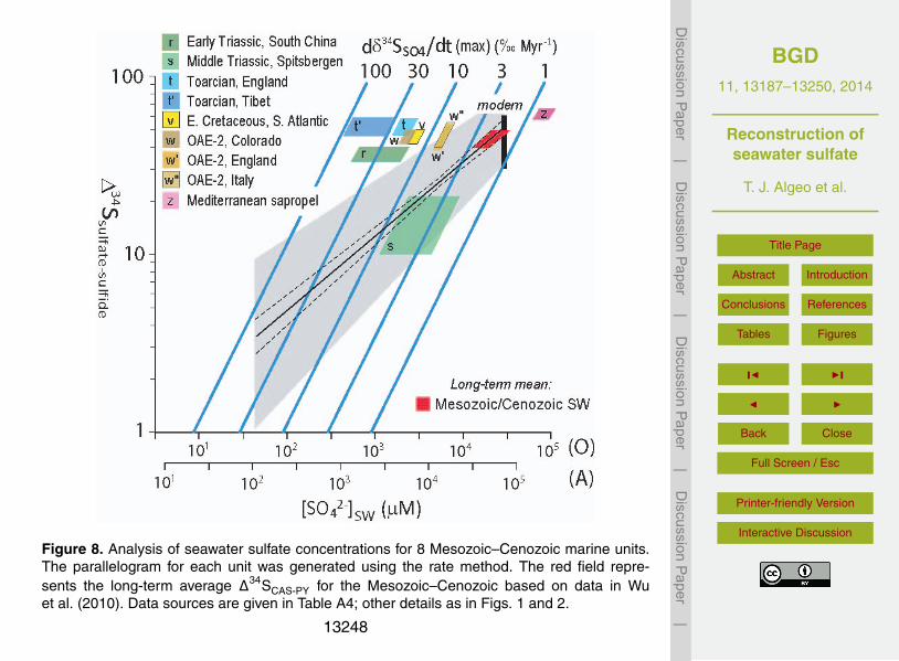
BGD11, 13187–13250, 2014


T. J. Algeo et al.

Title Page



Tables Figures

J I

J I

Back Close

Full Screen / Esc



Discussion

Paper

|D

iscussionP

aper|

Discussion

Paper

|D

iscussionP

aper|

Figure 8. Analysis of seawater sulfate concentrations for 8 Mesozoic–Cenozoic marine units.The parallelogram for each unit was generated using the rate method. The red field repre-sents the long-term average ∆34SCAS-PY for the Mesozoic–Cenozoic based on data in Wuet al. (2010). Data sources are given in Table A4; other details as in Figs. 1 and 2.

13248





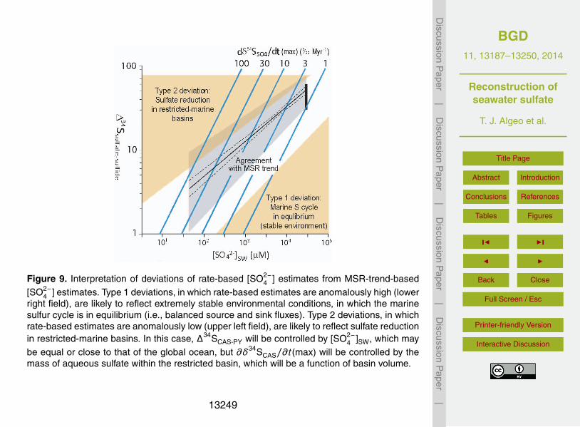
BGD11, 13187–13250, 2014


T. J. Algeo et al.

Title Page



Tables Figures

J I

J I

Back Close

Full Screen / Esc



Discussion

Paper

|D

iscussionP

aper|

Discussion

Paper

|D

iscussionP

aper|

Figure 9. Interpretation of deviations of rate-based [SO2−4 ] estimates from MSR-trend-based

[SO2−4 ] estimates. Type 1 deviations, in which rate-based estimates are anomalously high (lower

right field), are likely to reflect extremely stable environmental conditions, in which the marinesulfur cycle is in equilibrium (i.e., balanced source and sink fluxes). Type 2 deviations, in whichrate-based estimates are anomalously low (upper left field), are likely to reflect sulfate reductionin restricted-marine basins. In this case, ∆34SCAS-PY will be controlled by [SO2−

4 ]SW, which maybe equal or close to that of the global ocean, but ∂δ34SCAS/∂t(max) will be controlled by themass of aqueous sulfate within the restricted basin, which will be a function of basin volume.

13249





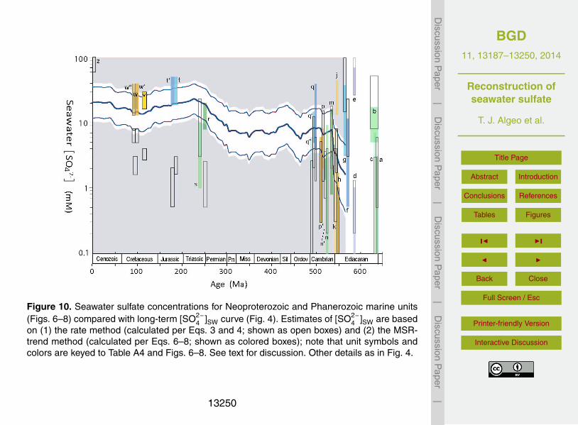
BGD11, 13187–13250, 2014


T. J. Algeo et al.

Title Page



Tables Figures

J I

J I

Back Close

Full Screen / Esc



Discussion

Paper

|D

iscussionP

aper|

Discussion

Paper

|D

iscussionP

aper|

Figure 10. Seawater sulfate concentrations for Neoproterozoic and Phanerozoic marine units(Figs. 6–8) compared with long-term [SO2−

4 ]SW curve (Fig. 4). Estimates of [SO2−4 ]SW are based

on (1) the rate method (calculated per Eqs. 3 and 4; shown as open boxes) and (2) the MSR-trend method (calculated per Eqs. 6–8; shown as colored boxes); note that unit symbols andcolors are keyed to Table A4 and Figs. 6–8. See text for discussion. Other details as in Fig. 4.

13250





Reconstruction of secular variation in seawater sulfate concentrations (2014, Biogeosciences Discussions)

Documents