Reconstructing Cortical Networks: Case of Directed Graphs with High Level of Reciprocity

Reconstructing Cortical Networks:Case of Directed Graphs with HighLevel of Reciprocity

Tamas Nepusz, Laszlo Negyessy, Gabor Tusnady, and Fulop Bazso

Abstract The problem of prediction of yet uncharted connections in thelarge scale network of the cerebral cortex is addressed. Our approach was de-termined by the fact that the cortical network is highly reciprocal althoughdirected, i.e. the input and output connection patterns of vertices are slightlydifferent. In order to solve the problem of predicting missing connections inthe cerebral cortex, we propose a probabilistic method, where vertices aregrouped into two clusters based on their outgoing and incoming edges, andthe probability of a connection is determined by the cluster affiliations of thevertices involved. Our approach allows accounting for differences in the in-coming and outgoing connections, and is free from assumptions about graphproperties. The method is general and applicable to any network for which theconnectional structure is mapped to a sufficient extent. Our method allowsthe reconstruction of the original visual cortical network with high accuracy,which was confirmed after comparisons with previous results. For the firsttime, the effect of extension of the visual cortex was also examined on graphreconstruction after complementing it with the subnetwork of the sensori-

Tamas Nepusz

KFKI Research Institute for Particle and Nuclear Physics of the Hungarian Academy ofSciences, H-1525 Budapest, P.O. Box 49., Hungary and Budapest University of Technology

and Economics, Department of Measurement and Information Systems, H-1521 Budapest,

P.O. Box 91., Hungary, e-mail: [email protected]

Laszlo NegyessyNeurobionics Research Group, Hungarian Academy of Sciences – Peter Pazmany Catholic

University – Semmelweis University, H-1094 Budapest, Tuzolto u. 58., Hungary

Gabor TusnadyAlfred Renyi Institute of Mathematics, Hungarian Academy of Sciences, Realtanoda u.

13-15., 1053 Budapest, Hungary

Bazso Fulop

KFKI Research Institute for Particle and Nuclear Physics of the Hungarian Academy ofSciences, H-1525 Budapest, P.O. Box 49., Hungary and Polytechnical Engineering College

Subotica, Marka Oreskovica 16, 24000 Subotica, Serbia, e-mail: [email protected]

1

2 Tamas Nepusz, Laszlo Negyessy, Gabor Tusnady, and Fulop Bazso

motor cortex. This additional connectional information further improved thegraph reconstruction. One of our major findings is that knowledge of defi-nitely nonexistent connections may significantly improve the quality of pre-dictions regarding previously uncharted edges as well as the understandingof the large scale cortical organization.

1 Introduction

The cerebral cortex is probably the most prominent example of a naturalinformation processing network. It is therefore of major importance to learnhow this network is organized. At the lowest level, the cortical network iscomposed of physically (i.e. via chemical and electrical synapses) connectednerve cells. (The chemical synapse is the dominant type and it is rectifying incontrast to the electrical synapse, which allows bi-directional interactions be-tween the neurons). The cortex, in general (ignoring species and areal densitydifferences [16]) consists of approximately 1010 nerve cells, each receiving nu-merous connections of order 103 (up to about 104) [7]. However, these data donot necessarily imply a homogenous degree distribution as the diverse typesof neurons could form specific sub-networks. Based on functional constraintsand axonal wiring economy, Buzsaki et al. [10] proposed a scale-free-like,small world architecture for the network of inhibitory local circuit neuronsconsisting approximately 20% of the whole neuron population. In fact, thesignificance of such a diversity of neurons is presently unknown, especiallyin the case of the pyramidal cells, which is the principal cell type of thecerebral cortex (making up the remaining 80%) [16]. Pyramidal cells, con-sidered excitatory in nature, form long distance connections both within thecortex and with subcortical structures. However, most of the synaptic con-tacts are formed locally within a short distance, and it is unclear how thecortical network is organized at the neuron level [18]. Considering anatomi-cal and physiological data, Tononi et al. [66] outlined a network architecture,which suitably performs segregation and integration, the fundamental func-tions of the central nervous system. Integration is achieved by connectionsbetween clusters of neurons, representing functionally specialized units, whichare formed by dense local connectivity [66]. Using mutual information as ameasure of integration, it was shown that the proposed network exhibitedhigh complexity, significantly differing from random and regular lattice net-works characterized by low measure of complexity [66]. Differences betweencortical and random networks were also pointed out by Negyessy et al. [46],although on the level of cortical areas instead of single neurons. On the otherhand, based on estimates of the spreading function, Bienenstock [6] showedthat the graph of cortical neurons has a high dimensionality close to that ofan Erdos-Renyi random graph of similar size. This assumption is consonantwith Szentagothai’s notion of quasi-randomness in neuronal connectivity [64].

Reconstructing Cortical Networks 3

The neuron doctrine (stating that nerve cells are the developmental, struc-tural and functional units of the central nervous system) has been challengedby arguing that populations of neurons function as units [5,8,19,23,44,63,66].This perspective is in close agreement with the so-called columnar or modu-lar organization of cortical structure and function as proposed by Mountcas-tle [44] and Szentagothai [63]. Accordingly, the cortex is usually viewed asa two dimensional sheet composed of functional modules with a diameter of250–500 µm, arranged perpendicularly to the surface and spanning the layersto the depth of the cortex. Although it is hard to estimate due to the dif-ferent types (and size) of columns [11, 44], a network of such modules wouldform a graph with millions of vertices in case of humans. Unfortunately, sucha network would be hard to draw because apart from some cortical regionsand specific columns (e.g., [4, 9, 35, 56, 57, 61]) the interconnections amongthese modules or cell clusters are obscure. In addition, functional modulesmay not be fixed structures; they could dynamically change their extensionvia neuronal plasticity (e.g., [11,31]). It is noteworthy that the minicolumnarorganization apparently can not resolve the problem of defining structuraland functional cortical units, as momentarily the minicolumn seems to be asimilarly vague concept as the column [18,55].

At a higher organizational level, the cortex is composed of a set (about ahundred, roughly four orders of magnitude less than the number of columnarmodules in the human) of structurally and functionally specialized regions orareas with highly variable shapes and sizes [67]. This level of organization isof great interest because the available anatomical and imaging (fMRI, PET,EEG, MEG) techniques made it possible to investigate the network of corticalareas (hence neuro-cognitive functions) [1, 8, 29, 41, 50]. Most of our knowl-edge about this large-scale cortical network comes from studies charting theneuronal connections between cortical areas. Since the use of sensitive andpowerful tract tracing techniques is not feasible in humans, the neural con-nections among the areas (“anatomical connectivity”, [59]) have been studiedintensely in non-human primates, especially in the macaque, which serves asa model of the human cortex [67]. Large collections of such data are availableat the CoCoMac database [37] and for updates, one may search PubMed [52].Although the areas are connected to each other via varying density of bun-dles of axonal processes [27] in a complicated laminar and topographicalpattern [20, 54], the network of areas is usually represented in binary formconsidering only the knowledge of the existence of a connection between theareas [58]. Even such a simplification allowed the description of the funda-mental properties of the network of cortical areas, e.g., its small-world likecharacteristics and hierarchical organization [28,32,59]. However, Kotter andStephan [38] have pointed out that the lack of information about connectivitycan hinder the understanding of important features of the cortical network.

The cortical network is directed, as long-range connections between the ar-eas end up in chemical synapses, but strongly reciprocal (reciprocity reaches80%) [20]. From the graph theoretic point of view, the high level of reci-


procity presents an obstacle by obscuring directedness in the network. Theglobal edge density is roughly 0.2–0.4 [58]. A granular organization repre-senting functional segregation and integration is prevalent also at this largescale [26,30,45,47,68], resulting in the density of connections going up to 0.6or more within the clusters [21]. The other major characteristic that makesthe cortex a small-world network is that its clustered organization is accom-panied by a short average path length, roughly between 2 and 3 [32, 59].Because it is reasonable to assume that a considerable part of the large-scalecortical network is still unknown, the identification of the key topologicalfeatures that characterize this network, i.e. understanding its organizationalprinciples, remained an open issue [21,30,33,34,38,51,60]. A practical way ofapproaching this problem is to check how exactly the network can be recon-structed by using a given index or network measure [21, 30]. This approachalso has the interesting consequence of predicting missing data, which can beverified experimentally. The two studies published up to now present data onsuch predictions of yet unknown connections in the cortex [21, 30]. The re-sults of these studies (especially those by Costa et al. [21], who investigateda broad set of measures) suggest that connectional similarity of the areasis a good predictor in reconstructing the original cortical network. However,they also report a relatively large number of violations, where known existentconnections were predicted as nonexistent in the reconstructed graphs andvice versa [21, 30]. This suggests that using other approaches could result inbetter reconstruction of the cortical network. The aim of the present studywas therefore to find a reconstruction algorithm that predicts the large-scalecortical network more accurately, i.e. with fewer violations. By consideringthe similarity of the connections of the individual areas, our approach is remi-niscent to that used by the previous analyses [21,30]. However, there are sub-stantial differences as well, especially the fact that we use a stochastic methodwhich is able to take into account the amount of uncertainty present in thedata being analyzed. Furthermore, contrary to the previous studies [21, 30],where the in- and outputs are either taken into account separately [30] or thenetwork was symmetrized prior to analysis [21], our approach is principallydependent on the combination of the areas’ in- and output pattern. Notably,considering the similarity of the in- and output pattern as the result of thehigh number of reciprocated links, a stochastic approach seems advantageous.Finally, in contrast to Jouve et al. [30], who assumed that a large number ofindirect connections of path length 2 is suggestive of the existence of a directlink between the areas, our method is free of such assumptions.

2 Methods

In this section, we introduce a simple stochastic graph model based on vertextypes and connection probabilities depending on them. From now on, we call


this the preference model. We will discuss a greedy and a Markov chain MonteCarlo (MCMC) method for fitting the parameters of the preference model to anetwork being studied. The MCMC method shows the rapid mixing property.In Section 3, we will employ these methods to reconstruct the cortical networkand to predict previously unknown connections.

2.1 General remarks on the method

The problem we would like to solve and the proposed method are not cor-tex specific, though the data on which we operate is. As data collectionand mapping are necessarily partial due to unavoidable observational errors,our method offers the possibility to map interactions, connections, influencesbased on the previous knowledge. Given the rough, but in principle correctsummary of such information in the form of appropriate graph model, onemay refine the knowledge of underlying graph represenation to some extent.Applications and extensions of the solution we propose are straightforwardto apply to any other network, with appropriate caution. The main assump-tions underlying our approach are as follows: the number of nodes is known inadvance, we only wish to predict previously uncharted edges, the majority ofthe edges are known, yet a large number of undetected edges are possible, atleast in principle. As with most problems involving prediction, it is relativelysimple to create a model performing slightly better than random tossing, butincreasing prediction accuracy is a difficult problem. Our approach to edgeprediction is inspired by one of the most influential results of graph theory byEndre Szemeredi [36, 62, 65], which became known as Szemeredi’s regularitylemma. Loosely speaking, the regularity lemma states that the structures ofvery large graphs can be described by assigning vertices to a small numberof almost equally sized groups and specifying the connection probabilitiesbetween the groups. The regularity lemma is formulated as an asymptoticaland existential statement. The graph we work with is definitely small, notcomparable in size to those graphs to which one would in principle applythe regularity lemma. Thus our model can be viewed as a form of fitting,with allowance for error. We do not try to pretend that the assumptions ofthe regularity lemma apply to the case of large-scale cortical networks, butthe idea underlying the regularity lemma, i.e. the probabilistic description ofconnections between and inside vertex groups, is exercised in order to find agood reconstruction. The proposed solution of the graph partitioning problemand its usage in edge prediction is achieved by using probabilistic methods,which allow finding solutions close to the optimum and satisfy the precisiondictated by the practical applications.


(a) (b)

Fig. 1 Two graphs generated by the preference model. Black and white colours denote

the groups the nodes belong to. Panel (a) shows a clustered graph where the connectionprobability between nodes within the same group is 0.2, while the connection probability

between nodes in different groups is only 0.02. Panel (b) shows a bipartite graph where

only nodes in different groups are allowed to connect with a probability of 0.2.

2.2 The preference model

This graph model starts from an empty graph with N vertices and it assignsevery vertex to one of K distinct groups. The groups are denoted by integernumbers from 1 up to K. The generation process considers all pairs of verticesonce, and it adds an edge between node v1 and v2 with probability pij if v1belongs to group i and v2 belongs to group j. That is, the expected densityof edges between group i and group j is exactly pij , and the existence ofan edge between two vertices depends solely on the group affiliation of thevertices involved. Fig. 1 shows two possible graphs generated by this model.The one shown on Fig. 1(a) is a graph with clustered organization: verticesin similar groups tend to link together while rarely linking to vertices of theother group. The graph on Fig. 1(b) is a bipartite graph. The model allowsthe simultaneous appearance of these two basic patterns in a graph: pii ≈ 1results in the one seen on Fig. 1(a) and pij ≈ 1, i 6= j induces the one onFig. 1(b). A method using similar ideas but designed for different applicationswas also described in a recent paper of Newman and Leicht [49].

The generalization of the model to directed graphs is straightforward: ver-tices of a directed graph will be assigned to an incoming and an outgoinggroup (in-group and out-group in short), and the probability of the existenceof an edge between a vertex from out-group i and another vertex from in-group j is given by pij . The number of parameters in this model isK2+2N+1,since there are 2N parameters for the group affiliations of the vertices, K2

parameters represent the elements of the preference matrix and the last pa-


rameter is K itself. The probabilities are usually arranged in a probabilitymatrix P for the sake of convenience. To emphasize the role of direction-ality, elements of the preference matrix in the directed case are sometimesdenoted by pi→j instead of pij . We also introduce the membership vectorsu = [u1, u2, . . . , uN ] and v = [v1, v2, . . . , vN ], where ui is the out-group andvi is the in-group of vertex i. From now on, parameterizations of the modelwill be denoted by M = (K,u,v,P).

This model naturally gives rise to densely connected subnetworks withsparse connections between them by appropriately specifying the connectionprobabilities within and between groups. This is a characteristic property ofcortical networks, and it is assumed that a good reconstruction of the net-work can be achieved by specifying vertex groups and connection probabili-ties appropriately. More precisely, given a graph G(V,E) without multiple orloop edges, the reconstruction task is equivalent to specifying the number ofgroups, finding an appropriate assignment of vertices to groups and determin-ing the elements of the probability matrix P. The reconstructed graph thencan be generated by the preference model, and new (previously unknown)connections can also be predicted by checking the probabilities of the uncer-tain edges in the fitted model. E.g., a crude reconstruction of the visuo-tactilenetwork of the macaque monkey (see Section 3 for details about this dataset)would be a model with two groups (group 1 corresonding to the visual andgroup 2 to the tactile vertices in the network) and connection probabilitiesp1→1 = 0.385, p1→2 = 0.059, p2→1 = 0.035 and p2→2 = 0.377, based on thedensity of connections between the groups in the original network. The intro-duction of more vertex types results in a better reconstruction, and obviouslythe reconstruction is perfect when N = K and P is A, the adjacency matrixof the graph. However, such a reconstruction is not able to predict unknownconnections. We will discuss the problem of overfitting in Section 2.5.

2.3 Measuring the accuracy of reconstruction

Since the preference model is a probabilistic model, every possible graph withN vertices can theoretically be generated by almost any parameterization ofthe model, but of course some graphs are more likely to be generated by aspecific parameterization than by others. Therefore, we measure the fitnessof a particular parameterization M = (K,u,v,P) with respect to a givengraph G(V,E) by its likelihood, i.e. the probability of the event that theprobabilistic model with parameters M generates G(V,E):

L(M|G) =∏

(i,j)∈E

pui→vj

∏(i,j)/∈E

i 6=j

(1− pui→vj) (1)


The restriction i 6= j in the second product term corresponds to the nonex-istence of loop edges (even if they exist, they are ignored). To avoid numericalerrors when working with small probabilities, one can use the log-likelihoodinstead, for the log-likelihood attains its maximum at the sameM where thelikelihood does:

logL(M|G) =∑

(i,j)∈E

log pui→vj+

∑(i,j)/∈E

i 6=j

log(1− pui→vj) (2)

2.4 Fitting the preference model

Fitting a model to a given graph G(V,E) is equivalent to the maximumlikelihood estimation (MLE) of the parameters of the model with respectto the graph, i.e. choosing M in a way that maximizes logL(M|G). Sincethe number of possible group assignments is KN (where K is the numberof groups and N = |V | is the number of vertices), which is exponentialin N , direct maximization of logL(M|G) by an exhaustive search is notfeasible. An alternative, greedy approach is therefore suggested to maximizethe likelihood.

2.4.1 Greedy optimization

Starting from an initial configurationM(0) =(K,u(0),v(0),P(0)

), the greedy

optimization will produce a finite sequence of model parameterizationsM(0),M(1), M(2), . . . satisfying L(M(k)|G) ≥ L(M(k−1)|G) for k ≥ 1. First wenote that the log-likelihood of an arbitrary configuration M is composed ofN local likelihood functions corresponding to the vertices:

logL(M|G) =N∑

i=1

N∑j=1j 6=i

log(Aijpui→vj + (1−Aij)

(1− pui→vj

))

=N∑

i=1

logLi(G|M) (3)

where Aij is 1 if there exists an edge from i to j and 0 otherwise. Let usassume first that K is given in advance. Starting from random initial mem-bership vectors u(0) and v(0) of M(0), we can estimate an arbitrary elementpi→j of the real underlying probability matrix P by counting the numberof edges that originate from out-group i and terminate in in-group j anddivide it by the number of possible edges between out-group i and in-groupj. The estimated probabilities are stored in P(0). After that, we examine


the local likelihoods Li(G|M(0)) for all vertices and choose the in- and out-groups of the vertices in a way that greedily maximizes their local likelihood,assuming that the group affiliations of all other vertices and the estimatedprobabilities remain unchanged. Formally, let u(0)

i=k denote the vector ob-tained from u(0) by replacing the ith element with k and similarly let v(0)

i=l

denote the vector obtained from v(0) by replacing the ith element with l.LetM(0)

i,k,l =(K,u(0)

i=k,v(0)i=l,P

(0))

, and for every vertex i, every out-group k

and every in-group l, calculate logLi(G|M(0)i,k,l). After that, put vertex i in

out-group k and in-group l if that maximizes logLi(G|M(0)i,k,l). Now calcu-

late the next estimation of the probability matrix, P(1), maximize the locallog-likelihoods based on the new probability matrix and repeat these twoalternating steps until u(k) = u(k−1) and v(k) = v(k−1).

2.4.2 Markov chain Monte Carlo sampling

The group assignments obtained by the greedy algorithm suffer from a minorflaw: they correspond only to a local maximum of the parameter space andnot the global one. The local maximum means that no further improvementcould be made by putting any single vertex in a different group while keepingthe group affiliations of all other vertices intact. However, there is the pos-sibility of improving the partition further by moving more than one vertexsimultaneously. Another shortcoming of the algorithm is the danger of over-fitting: partitions with high likelihood might perform poorly when one triesto predict connections, because they are too much fine-tuned to the graphbeing analyzed. Therefore we also consider employing Markov chain MonteCarlo (MCMC) sampling methods [3] on the parameter space. (An alterna-tive MCMC-based data mining method on networks is presented in [13], butwhile that method infers hierarchical structures in networks, our algorithmis concerned with the discovery of densely connected subgraphs and bipartitestructures; see Fig. 1(a) and Fig. 1(b), respectively).

Generally, MCMC methods are a class of algorithms for sampling froma probability distribution that is hard to be sampled from directly. Thesemethods generate a Markov chain whose equilibrium distribution is equivalentto the distribution we are trying to sample from. In our case, the samplesare parameterizations of the preference model, and the distribution we aresampling from is the following:

P(M =M0) =L(M0|G)∫

SK

L(M′|G) dM′(4)


where SK is the space of all possible parameterizations of the probabilitymodel for a given K. Informally, the probability of drawing M as a sampleshould be proportional to its likelihood of generating G(V,E), for instance,if M1 generates our network with a probability of 0.5 and M2 generates itwith a probability of 0.25, M1 should be drawn twice as frequently as M2.

The generic framework of the MCMC method we use is laid down inthe Metropolis-Hastings algorithm [25]. The only requirement of the al-gorithm is that a function proportional to the density function (that is,P(M =M0) in (4)) can be calculated. Note that P(M =M0) ∝ L(M0|G),since the denominator in (4) is constant. Starting from an arbitrary ran-dom parameterization M(0), MCMC methods propose a new parameteri-zation M′ based on the previous parameterization M(t) using a proposaldensity function Q(M′|M(t)). If the proposal density function is symmet-ric (Q(M′|M(t)) = Q(Mt|M′)), the probability of accepting the proposedparameterization is min

(1, L(M′|G)/L(M(t))

∣∣G). When the proposal is ac-cepted, it becomes the next state in the Markov chain (M(t+1) = M′),otherwise the current state is retained (M(t+1) =M(t)).

MCMC sampling can only approximate the target distribution, since thereis a residual effect depending on the starting position of the Markov chain.Therefore, the sampling consists of two phases. In the first phase (calledburn-in), the algorithm is run for many iterations until the residual effectdiminishes. The second phase is the actual sampling. The burn-in phase mustbe run long enough so that the residual effects of the starting position becomenegligible.

A desirable property of a Markov chain in a MCMC method is rapid mix-ing. A Markov chain is said to mix rapidly if its mixing time grows at mostpolynomially fast in the logarithm of the number of possible states in thechain. Mixing time refers to a given formalization of the following idea: howmany steps do we have to take in the Markov chain to be sure that the distri-bution of states after these steps is close enough to the stationary distributionof the chain? Given a guaranteed short mixing time, one can safely decideto stop the burn-in phase and start the actual sampling after the number ofsteps taken exceeded the mixing time of the chain.

Several definitions exist for the mixing time of a Markov chain (for anoverview, see [43]). To illustrate the concept, we refer to a particular variantcalled total variation distance mixing time, which is defined as follows:

Definition 1 (Total variation distance mixing time). Let S denote theset of states of a Markov chain C, let A ⊆ S be an arbitrary nonempty subsetof the state set, let π(A) be the probability of A in the stationary distributionof C, and πt(A) be the probability of A in the distribution observed after stept. The total variation distance mixing time of C is the smallest t such that|πt(A)− π(A)| ≤ 1/4 for all A ⊆ S and all initial states.

However, many practical problems have resisted rigorous theoretical anal-ysis. This applies also to the method presented here, mostly due to the fact


that the state transition matrix of the Markov chain (and therefore its sta-tionary distribution) is a complicated function of the adjacency matrix of thenetwork and the number of vertex groups, and no closed form descriptionexists for either. In these cases, a common approach to decide on the lengthof the burn-in phase is based on the acceptance rate, which is the fraction ofstate proposals accepted during the last m steps. Sampling is started whenthe acceptance rate drops below a given threshold (a typical choice is 20% or0.2). Local maxima are avoided by accepting parameterization proposals witha certain probability even when they have a lower likelihood than the last one,but being biased at the same time towards partitions with high likelihoods.In the case of multiple local maxima with approximately the same likelihood,MCMC sampling tends to oscillate between those local maxima. By takinga large sample from the equilibrium distribution, one can approximate theprobability of vertex i being in out-group k and in-group l and extract thecommon features of all local maxima (vertices that tend to stay in the samegroups despite randomly walking around in the parameter space).

The only thing left to clarify before employing MCMC sampling on fittingthe preference model is the definition of an appropriate symmetric proposaldensity function. We note that the number of groups K is constant and theprobability matrix P can be approximated by the edge densities for a givenout- and in-group assignment, leaving us with only 2N parameters that haveto be determined. We take advantage of the fact that the conditional distri-bution of each parameter (assuming the others are known) can be calculatedexactly as follows:

P(ui = k) =Li(G|Mi,k,∗)∑Kl=1 Li(G|Mi,l,∗)

(5a)

P(vi = k) =Li(G|Mi,∗,k)∑Kl=1 Li(G|Mi,∗,k)

(5b)

where Mi,k,∗ = (K,ui=k,v,P) and Mi,∗,k = (K,u,vi=k,P). Since the con-ditional distribution of each parameter is known, Gibbs sampling [24] can beused. The Gibbs sampling alters a single variable of the parameter vector ineach step according to its conditional distribution, given all other parameters.It can be shown that the proposal distribution defined this way is symmet-ric if the variable being modified is picked randomly according to a uniformdistribution. In practice, it is sufficient to cycle through the variables in apredefined order as long as the Markov chain can access all states under thisordering. To speed up the burn-in process, one can apply the greedy optimiza-tion method described in Section 2.4.1 and revert to the MCMC samplingwhen the algorithm reached the first local maximum.


2.5 Choosing the number of groups

As mentioned earlier in Section 2.2, the key parameter that controls thebalance between accurate reconstruction and meaningful prediction is thenumber of vertex groups used in the preference model. A very small numberof groups yields an inaccurate reconstruction and most likely meaninglesspredictions. Increasing the number of groups gradually improves the accuracyof reconstruction, attaining perfection when the number of groups is equalto the number of vertices, but in this case no new edges are predicted. Thisis the classical problem of overfitting: by increasing the number of groups,the ability of the model to generalize beyond the original data diminishes.Therefore, the goal is to select the number of groups in a way that achievesgood reconstruction while still allowing the model to predict connections byassigning a high probability to vertex pairs where an uncertain connection issuspected.

We tried multiple approaches to infer the appropriate number of groups inthe networks we studied. The exact results will be discussed in Section 2.6.2and Section 3; here we only outline the basic ideas. We will make use of theeigenvalues of the Laplacian matrix of the graph, the singular value decompo-sition (SVD) of the adjacency matrix and the Akaike information criterion [2].

Given an undirected graph G(V,E) without loops and multiple edges, itsLaplacian matrix is defined as L = D−A, where A is the adjacency matrixand D is a diagonal matrix composed of the degrees of the vertices. A basicproperty of the Laplacian matrix is that its smallest eigenvalue is zero, andits multiplicity is equal to the number of connected components of the graph.The number of eigenvalues close to zero is frequently used for determiningthe number of dense subgraphs (communities, clusters) in the graph and,based on similar reasoning, this could be a good estimate of the number ofgroups that have to be used in the preference model; however, we cannot useD−A directly, since this form of the Laplacian is defined only for undirectedgraphs.

An extension of the Laplacian to directed graphs was introduced in [12].This involves calculating the Perron vector φ of the transition probabilitymatrix P of the graph. The transition probability matrix P is derived fromthe adjacency matrix by normalizing the row sums to be 1. The Perron vectorφ is a unique (up to scaling) left eigenvector of P satisfying φP = φ. Theexistence of this vector is guaranteed by the Perron-Frobenius theorem. Thereis no closed-form solution for φ, but it is easy to calculate in polynomial timenumerically. The directed Laplacian is then defined as:

L = I− Φ1/2PΦ−1/2 + Φ−1/2P∗Φ1/2

2(6)


where P∗ is the conjugate transpose of P and Φ is a diagonal matrix composedof the elements of φ, assuming that

∑ni=1 φi = 1. The properties emphasized

above for the undirected Laplacian hold for the directed Laplacian as well.The singular value decomposition of an m×n matrix M is a factorization

process that produces an m × m and an n × n unitary matrix (U and V,respectively) and an m × n matrix Σ with non-negative numbers on thediagonal and zeros off the diagonal in a way that M = UΣV∗. The diagonalof Σ contains the singular values, while the columns of U and V are theleft and right singular vectors, respectively. Plotting the singular values ona scree plot (sorted from large to small) is a good visual cue to determiningthe number of groups in the model: the number of groups can simply beassigned according to the number of large singular values. It is noteworthythat one can approximate the original matrix M by setting all singular valuesother than the l largest to zero and disregarding the appropriate rows of Uand V that correspond to the zeroed singular values. The remaining partsof U and V can serve as an input for a k-means clustering algorithm in anl-dimensional space, and the results of the clustering yield a good candidateof an initial position of the greedy optimization process of the preferencematrix. In practice, however, performing a complete SVD is less efficientthan optimization from a random initial position.

The Akaike information criterion (AIC) [2] is a measure of the goodness offit of a statistical model (the preference model in our case). It is an unbiasedestimator of the Kullback-Leibler divergence [39], and it is an operational wayof determining the appropriate trade-off between the complexity of a modeland its predictive power. AIC is calculated as 2k − 2 logL, where k is thenumber of parameters in the model and L is the likelihood. In the preferencemodel, k = K2 +2N+1. The suggested number of groups can be determinedby fitting the model with various numbers of groups and choosing the onethat minimizes the Akaike information criterion.

The AIC can also be used to detect situations when the network beingstudied is in fact completely random, and therefore its appropriate descriptionis simply an Erdos–Renyi random graph model instead of the preferencemodel. This is done by estimating the probability parameter p of the Erdos–Renyi model from the edge density of the network and then calculating thelog-likelihood of the network according to the Erdos–Renyi model. Givena directed network with n vertices and m edges, the maximum likelihoodestimator of p is m

n(n−1) , resulting in a log-likelihood of m log p + (n2 − n −m) log(1 − p) (assuming that there are no loop edges). The baseline AICcorresponding to the Erdos–Renyi model is then 2 − 2(m log p + (n2 − n −m) log(1 − p)), since the model has only a single parameter. If the networkbeing studied is completely random, the AIC corresponding to the case of twogroups will be larger than the baseline AIC of the Erdos–Renyi model, forwe introduced more parameters without actually improving the likelihood.On the other hand, networks possessing a structure that can be described by


the preference model will show significant improvement in the log-likelihoodcompared to the pure random case, resulting in a lower AIC.

2.6 Performance measurements

To demonstrate the validity of the fitting algorithms presented above, weconducted several benchmarks on computer-generated test graphs. First, wegenerated graphs according to the preference model, ran the fitting algorithmon the graphs by supplying the appropriate number of groups beforehandand then compared the known and the estimated parameters of the model.These benchmarks were performed in order to test the validity of the fittingalgorithm and to assess the quality of the results obtained. Next, we ran thefitting algorithms without specifying the number of groups to show that theAkaike information criterion is suitable for determining the right value of k.

2.6.1 Fitting the model with given number of groups

This benchmark proceeded as follows: graphs with 128 vertices were gener-ated according to the preference model using 4 in- and out-types. The typedistribution was uniform, so there were 32 vertices of each type on average.The preference matrix was chosen as follows: each element pij was set toone of two predefined values p1 and p2 with probability 0.5. p1 and p2 wasvaried between 0 and 1 with a step size 0.05. For each (p1, p2) combination,we generated 50 graph instances using the preference model. Values of thequality functions (described below) were averaged over these instances andthe results were plotted as a function of p1 and p2. We used only two prob-abilities because the results can then be visualized on a heat map or a 2.5Dplot.

To assess the fitness of the fitted model, we had to define some qualityfunctions that compare the fitted parameters to the original (expected) ones.First we note that the number of groups and the probability matrix do nothave to be compared, since the former is fixed and the latter one is calculatedfrom the group assignments, so errors in the elements of the probability ma-trices are simply due to errors in the group assigments. Therefore, only thegroup assignments matter. The following quality functions were defined:

Normalized mutual information of the confusion matrix. This mea-sure was suggested by Fred and Jain [22] and later applied to communitydetection in graphs by Danon et al. [15]. The measure is based on the con-fusion matrix C = [cij ] of the expected and observed group assignments.cij is the number of vertices that are in group i in the original and groupj in the fitted model. The confusion matrix can be calculated separatelyfor in- and out-groups, but they can safely be added together to obtain


a single confusion matrix and then a single quality measure, which is thenormalized mutual information of the confusion matrix:

I(C) = −2

∑ki=1

∑kj=1 cij log cijc∗∗

ci∗c∗j∑ki=1

(ci∗ log ci∗

c∗∗+ c∗i log c∗i

c∗∗

) (7)

where ci∗ is the sum of the i-th row, c∗j is the sum of the j-th column ofthe confusion matrix. c∗∗ is the sum of cij for all i, j. It is assumed that0 log 0 = 0. When the fitted group assignment is completely identical to theexpected one (apart from rearrangement of group indices), I(C) attainsits maximum at 1. I(C) = 0 if the two group assignments are indepen-dent. Danon et al. [15] argue that this measure is in general stricter thanmost other quality measures proposed so far. For instance, a completelyrandom assignment of groups still has an expected success ratio of 0.25for 4 groups (since each pair is consistent with probability 1/4). In thiscase, the normalized mutual information is close to zero, which is a moreintuitive description of what happened than a success ratio of 0.25. Seethe paper of Danon et al. [15] for a list of other measures they considered.

Likelihood ratio. This measure is simply the ratio of the likelihoods ofthe original and the fitted parameterizations, given the generated graph.

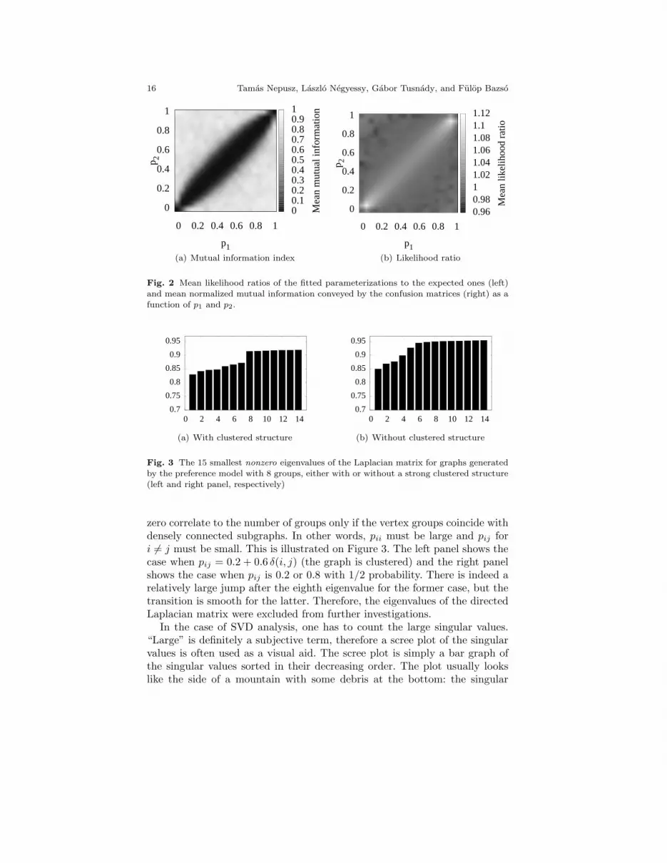
The likelihood ratios and the mutual information indices are plotted onFigure 2. As expected, the mutual information index is low when p1 ≈ p2.This is no surprise, since p1 ≈ p2 implies that the actual difference betweendifferent vertex types diminish: they all behave similarly, and the randomfluctuations at this network size render them practically indistinguishable.The overall performance of the algorithm is satisfactory in the case of p1 � p2

and p1 � p2, with success ratios and mutual information indices larger than0.9 in all cases. In cases when p1 ≈ p2, the likelihood ratio is greater than1, which indicates that the fitted model parameterization is more likely thanthe original one. This phenomenon is an exemplar of overfitting: apparentstructure is detected by the algorithm where no structure exists at all if weuse too many groups.

2.6.2 Fitting the model without a predefined number of groups

In Section 2.5, we described three different methods for estimating the num-ber of groups one should use for a given network when fitting the preferencemodel. Two of these methods requires some human intervention, since onehad to choose a threshold manually for the eigenvalues of the Laplacian ma-trix or for the singular values of the adjacency matrix.

We investigated the eigenvalues of the directed Laplacian matrix first. Af-ter some experiments on graphs generated according to the preference model,it became obvious that the number of eigenvalues of the Laplacian close to


0 0.1 0.2 0.3 0.4 0.5 0.6 0.7 0.8 0.9 1

Mea

n m

utua

l inf

orm

atio

n

0 0.2 0.4 0.6 0.8 1

p1

0

0.2

0.4

0.6

0.8

1

p 2

(a) Mutual information index

0.96 0.98 1 1.02 1.04 1.06 1.08 1.1 1.12

Mea

n lik

elih

ood

ratio

0 0.2 0.4 0.6 0.8 1

p1

0

0.2

0.4

0.6

0.8

1

p 2

(b) Likelihood ratio

Fig. 2 Mean likelihood ratios of the fitted parameterizations to the expected ones (left)and mean normalized mutual information conveyed by the confusion matrices (right) as a

function of p1 and p2.

0.7 0.75 0.8

0.85 0.9

0.95

0 2 4 6 8 10 12 14

(a) With clustered structure

0.7 0.75

0.8 0.85

0.9 0.95

0 2 4 6 8 10 12 14

(b) Without clustered structure

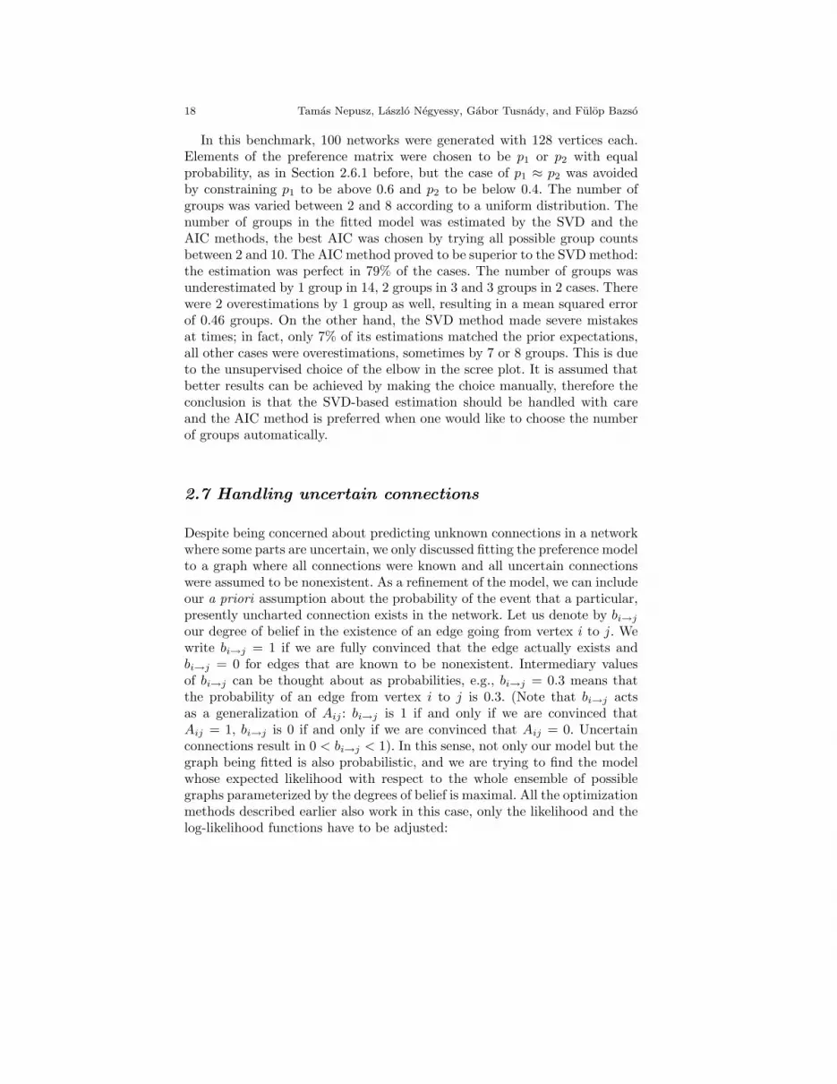
Fig. 3 The 15 smallest nonzero eigenvalues of the Laplacian matrix for graphs generated

by the preference model with 8 groups, either with or without a strong clustered structure

(left and right panel, respectively)

zero correlate to the number of groups only if the vertex groups coincide withdensely connected subgraphs. In other words, pii must be large and pij fori 6= j must be small. This is illustrated on Figure 3. The left panel shows thecase when pij = 0.2 + 0.6 δ(i, j) (the graph is clustered) and the right panelshows the case when pij is 0.2 or 0.8 with 1/2 probability. There is indeed arelatively large jump after the eighth eigenvalue for the former case, but thetransition is smooth for the latter. Therefore, the eigenvalues of the directedLaplacian matrix were excluded from further investigations.

In the case of SVD analysis, one has to count the large singular values.“Large” is definitely a subjective term, therefore a scree plot of the singularvalues is often used as a visual aid. The scree plot is simply a bar graph ofthe singular values sorted in their decreasing order. The plot usually lookslike the side of a mountain with some debris at the bottom: the singular


0 20 40 60 80

100 120

5 10 15 20

Fig. 4 The largest 20 singular values of the adjacency matrix of a graph generated by the

preference model with 8 groups

values decrease rapidly at first, but there is an elbow where the steepnessof the slope decreases abruptly, and the plot is almost linear from there on(see Figure 4 for an illustration). The number of singular values to the leftof the elbow is the number of groups we will choose. To allow for automatedtesting, we implemented a simple method to decide on the place of the elbow.The approach we used is practically equivalent to the method of Zhu andGhodsi [69]. It is based on the assumption that the values to the left andright of the elbow behave as independent samples drawn from a distributionfamily with different parameters. The algorithm first chooses a distributionfamily (this will be the Gaussian distribution in our case), then considers allpossible elbow positions and calculates the maximum likelihood estimationof the distribution parameters based on the samples to the left and right sideof the elbow. Finally, the algorithm chooses the position where the likelihoodwas maximal. Assuming Gaussian distributions on both sides, the estimatesof the mean and variance are as follows:

µ1 =∑q

i=1 xi

qµ2 =

∑ni=q+1 xi

n− q

σ2 =

∑qi=1 (xi − µ1)2 +

∑ni=q+1 (xi − µ2)2

n− 2

(8)

where xi is the i-th element in the scree plot (sorted in decreasing order),n is the number of elements (which coincides with the number of vertices)and q is the number of elements standing to the left of the elbow. Notethat the means of the Gaussian distributions are estimated separately, butthe variance is common. Zhu and Ghodsi [69] argue that allowing differentvariances makes the model too flexible. The common variance is calculatedby taking into account that the first q elements are compared to µ1 and theremaining ones are compared to µ2. See the paper of Zhu and Ghodsi [69] fora more detailed description of the method.


In this benchmark, 100 networks were generated with 128 vertices each.Elements of the preference matrix were chosen to be p1 or p2 with equalprobability, as in Section 2.6.1 before, but the case of p1 ≈ p2 was avoidedby constraining p1 to be above 0.6 and p2 to be below 0.4. The number ofgroups was varied between 2 and 8 according to a uniform distribution. Thenumber of groups in the fitted model was estimated by the SVD and theAIC methods, the best AIC was chosen by trying all possible group countsbetween 2 and 10. The AIC method proved to be superior to the SVD method:the estimation was perfect in 79% of the cases. The number of groups wasunderestimated by 1 group in 14, 2 groups in 3 and 3 groups in 2 cases. Therewere 2 overestimations by 1 group as well, resulting in a mean squared errorof 0.46 groups. On the other hand, the SVD method made severe mistakesat times; in fact, only 7% of its estimations matched the prior expectations,all other cases were overestimations, sometimes by 7 or 8 groups. This is dueto the unsupervised choice of the elbow in the scree plot. It is assumed thatbetter results can be achieved by making the choice manually, therefore theconclusion is that the SVD-based estimation should be handled with careand the AIC method is preferred when one would like to choose the numberof groups automatically.

2.7 Handling uncertain connections

Despite being concerned about predicting unknown connections in a networkwhere some parts are uncertain, we only discussed fitting the preference modelto a graph where all connections were known and all uncertain connectionswere assumed to be nonexistent. As a refinement of the model, we can includeour a priori assumption about the probability of the event that a particular,presently uncharted connection exists in the network. Let us denote by bi→j

our degree of belief in the existence of an edge going from vertex i to j. Wewrite bi→j = 1 if we are fully convinced that the edge actually exists andbi→j = 0 for edges that are known to be nonexistent. Intermediary valuesof bi→j can be thought about as probabilities, e.g., bi→j = 0.3 means thatthe probability of an edge from vertex i to j is 0.3. (Note that bi→j actsas a generalization of Aij : bi→j is 1 if and only if we are convinced thatAij = 1, bi→j is 0 if and only if we are convinced that Aij = 0. Uncertainconnections result in 0 < bi→j < 1). In this sense, not only our model but thegraph being fitted is also probabilistic, and we are trying to find the modelwhose expected likelihood with respect to the whole ensemble of possiblegraphs parameterized by the degrees of belief is maximal. All the optimizationmethods described earlier also work in this case, only the likelihood and thelog-likelihood functions have to be adjusted:


L(M|G) =N∏

i=1

N∏j=1,j 6=i

(bi→jpui→vj

+ (1− bi→j)(1− pui→vj

))(9a)

logL(M|G) =N∑

i=1

N∑j=1,j 6=i

log(bi→jpui→vj + (1− bi→j)

(1− pui→vj

))(9b)

The elements of the optimal probability matrix P can then be thoughtabout as the posterior probabilities of the edges in the network. An edgewhose prior probability is significantly lower than its posterior probability isthen likely to exist, while connection candidates with significatly higher priorthan posterior probabilities are likely to be nonexistent.

3 Results and discussion

In this section, we will present our results on application of the preferencemodel to the prediction of unknown connections in the visual and sensorimo-tor cortex of the primate (macaque monkey) brain.

The dataset we are concerned with in this section is a graph model ofthe visuo-tactile cortex of the macaque monkey brain. Connectivity data wasretrieved from the CoCoMac database [37] and it is identical to the datasetpreviously published in [45]. The whole network contains 45 vertices and463 directed links among them. The existence of connections included in thenetwork were confirmed experimentally, while connections missing from thenetwork were either explicitly checked for and found to be nonexistent, ornever checked experimentally. To illustrate the uncertainty in the datasetbeing analyzed, we note that 1157 out of the 1980 possible connections wereuncertain (never checked experimentally) and only 360 were known to beabsent.

The network consists of two dense subnetworks corresponding to the vi-sual and the sensorimotor cortex (30 and 15 vertices, respectively). The visualcortex can also be subdivided to the so-called dorsal and ventral parts usinga community detection algorithm based on random walks [40]. Most of theuncertain connection candidates are heteromodal (originating in the visualand terminating in the sensorimotor cluster, or the opposite), and it is as-sumed that the vast majority of possible heteromodal connections are indeednonexistent. The basic properties of these networks are shown in Table 1,while the adjacency matrix of the visuo-tactile network is depicted on Fig. 5.Note that since the visual and sensorimotor cortices are subnetworks of thevisuo-tactile networks, their adjacency matrices are the upper-left 30×30 andlower-right 15 × 15 submatrices of the adjacency matrix of the visuo-tactilecortex. In order to compare our results with previous reconstruction attemptsthat were only concerned with the visual cortex [21, 30], we will present re-sults based on the visual subnetwork as well as the whole visuo-tactile cortex.


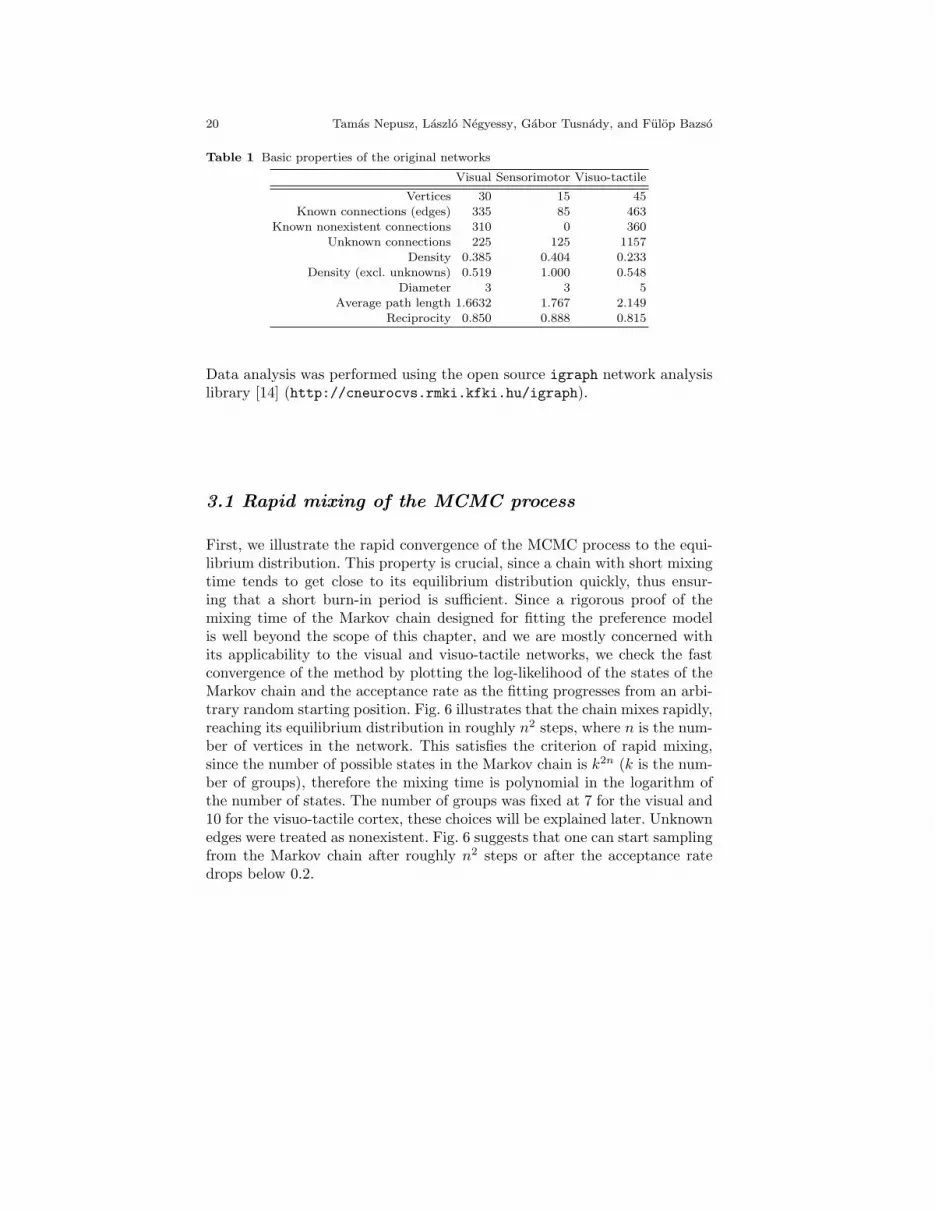
Table 1 Basic properties of the original networks

Visual Sensorimotor Visuo-tactile

Vertices 30 15 45

Known connections (edges) 335 85 463Known nonexistent connections 310 0 360

Unknown connections 225 125 1157

Density 0.385 0.404 0.233Density (excl. unknowns) 0.519 1.000 0.548

Diameter 3 3 5

Average path length 1.6632 1.767 2.149Reciprocity 0.850 0.888 0.815

Data analysis was performed using the open source igraph network analysislibrary [14] (http://cneurocvs.rmki.kfki.hu/igraph).

3.1 Rapid mixing of the MCMC process

First, we illustrate the rapid convergence of the MCMC process to the equi-librium distribution. This property is crucial, since a chain with short mixingtime tends to get close to its equilibrium distribution quickly, thus ensur-ing that a short burn-in period is sufficient. Since a rigorous proof of themixing time of the Markov chain designed for fitting the preference modelis well beyond the scope of this chapter, and we are mostly concerned withits applicability to the visual and visuo-tactile networks, we check the fastconvergence of the method by plotting the log-likelihood of the states of theMarkov chain and the acceptance rate as the fitting progresses from an arbi-trary random starting position. Fig. 6 illustrates that the chain mixes rapidly,reaching its equilibrium distribution in roughly n2 steps, where n is the num-ber of vertices in the network. This satisfies the criterion of rapid mixing,since the number of possible states in the Markov chain is k2n (k is the num-ber of groups), therefore the mixing time is polynomial in the logarithm ofthe number of states. The number of groups was fixed at 7 for the visual and10 for the visuo-tactile cortex, these choices will be explained later. Unknownedges were treated as nonexistent. Fig. 6 suggests that one can start samplingfrom the Markov chain after roughly n2 steps or after the acceptance ratedrops below 0.2.


V1V2V3

V3AV4V4tVOTVPMT

MSTd/pMSTlPOLIPPIPVIPDP7a

FSTPITdPITvCITdCITvAITdAITvSTPpSTPa

TFTHFEF463a3b125RiSII7b46

SMAIgId3536

V1

V2

V3

V3A

V4

V4t

VOT

VP

MT

MSTd/p

MSTl

PO LIP

PIP

VIP

DP

7a FST

PITd

PITv

CITd

CITv

AITd

AITv

STPp

STPa

TF TH FEF

46 3a 3b 1 2 5 Ri

SII

7b 4 6 SMA

Ig Id 35 36

XXXXXXXXXXXXXXXXXXXXXXXXXXXXXXXXXXXXXXXXXXXXX

Fig. 5 Adjacency matrix of the visuo-tactile cortex dataset. Black cells denote knownexisting connections, white cells denote known nonexistent connections. Gray cells are

connections not confirmed or confuted experimentally. The upper left 30 × 30 submatrix

is the adjacency matrix of the visual cortex, the lower right 15 × 15 submatrix describesthe sensorimotor cortex.

3.2 Methodological comparison with other predictionapproaches

Our method allows prediction of nonreciprocal connections, and the networkdata is not symmetrised for the sake of computational and methodologicaltractability, in contrast to [21]. Furthermore, we only use the connectionaldata for prediction,, no other anatomical facts were taken into account. Anapproach where additional neuroanatomical facts were used as predictionalinput is described in [21]. Jouve et al. [30] use a specific property of the visualcortex: the existence of indirect connections of length 2 between areas are


-1200

-1000

-800

-600

-400

10-4 10-3 10-2 10-1 100 101 102

log-

likel

ihoo

d

time / n2

Visual, n=30Visuotactile, n=45

0

0.2

0.4

0.6

0.8

1

10-4 10-3 10-2 10-1 100 101 102

acce

ptan

ce r

ate

time / n2

Visual, n=30Visuotactile, n=45

Fig. 6 Log-likelihood of the states of the Markov chain (left) and acceptance rates in a

window of 100 samples (right) for the visual and visuo-tactile cortices, normalised by n2,on a logarithmic time scale

presumed to support the existence of a direct connection. This property neednot hold for other large cortical structures, especially when investigating theinterplay of different cortices (e.g., the visual and the sensorimotor cortices).In fact, this assumption is difficult to prove or disprove due to the poorknowledge of connection structure in other parts of the cortex. The problemis even more pronounced in the case of heteromodal connections, thus otherguiding principles had to be sought.

3.3 Visual cortex

Since the visual cortex is a part of the visuo-tactile cortex, the adjacencygraph of the visual cortex can be found in Fig. 5 as the upper left 30 × 30submatrix. It is noteworthy that most of the unknown connections are adja-cent to the areas VOT and V4t, and the subgraph consisting of the verticesPITd, PITv, CITd, CITv, AITd, AITv, STPp and STPa (all belonging tothe ventral class) is also mostly unknown. Based on the connection densityof the visual cortex (assuming unknown connections to be nonexistent), theprobability of the existence of a connection classified as unknown was set to0.385. These degrees of belief were taken into account in the likelihood func-tion as described in Sect. 2.7. The search for the optimal configuration startedfrom a random initial position, first improved by a greedy initial phase, thenfollowed by MCMC sampling after reaching the first local maximum. Thesampling process was terminated when at least 106 samples were taken fromthe chain. The sample with the best likelihood became the final result.

The optimal number of groups in the preference model was determined bystudying the eigenvalues of the Laplacian and the singular values of the ad-


0

0.2

0.4

0.6

0.8

1

1.2

1.4

1.6

0 5 10 15 20 25 30

Eigenvalues

(a) Eigenvalues

0

2

4

6

8

10

12

14

0 5 10 15 20 25 30

Singular values

(b) Singular values

Fig. 7 Eigenvalues of the Laplacian and singular values of the adjacency matrix of thevisual cortical graph

jacency matrix (unknown connections were treated as nonexistent) as well asthe Akaike information criterion of the obtained partitions at various groupnumbers from 2 to 15. Partitions having more than 15 groups do not seemfeasible, since in these cases, at least one of the groups will contain only onevertex. The eigenvalues and the singular values are shown on Fig. 7. A vi-sual inspection suggests using only two groups (which is congruent with theanatomical fact that the visual cortex is composed of two major pathways,namely the dorsal and the ventral stream), but the minimal AIC value wasachieved using 7 groups (see Table 2). Since two groups are intuitively in-sufficient for an accurate reconstruction, we decided to use 7 groups in therest of the analysis. This is further supported by the mediocre success rate ofthe model with only two groups. Success rates were calculated as follows: forevery possible threshold τ between 0 and 1 (with a granularity of 0.01), thepercentage of known edges that had a predicted probability greater than τwas calculated. The final threshold used for calculating the success rate waschosen to be the one that produced the highest ratio of correctly predictedknown edges. τ fluctuated around 0.5 in all cases. As it was expected basedon our reasoning outlined in Sect. 2.5, the success rate increased steadily aswe increased the number of groups, but the divergence of τ from 0.5 afterhaving more than 7 groups is likely to be a precursor of overfitting.

The fitted model with 7 groups provided probabilities for the 225 unknownconnections, 137 of them were above the optimal threshold τ = 0.5. The ratioof predicted edges approximately matches the density of the visual cortexwhen we exclude the unknown connections from the density calculation (seeTable 1). However, if we wanted the ratio of predicted connections to matchthe density of known connections in the visual cortex, we would have toincrease τ to 0.654, predicting only 81 connections. This ratio matches the onereported in [21], although the connection matrix in [21] included an additionalarea in the analysis. The predicted adjacency matrix with τ=0.654 is shownon Fig. 8 and its basic descriptive graph measures are to be found in Table3.


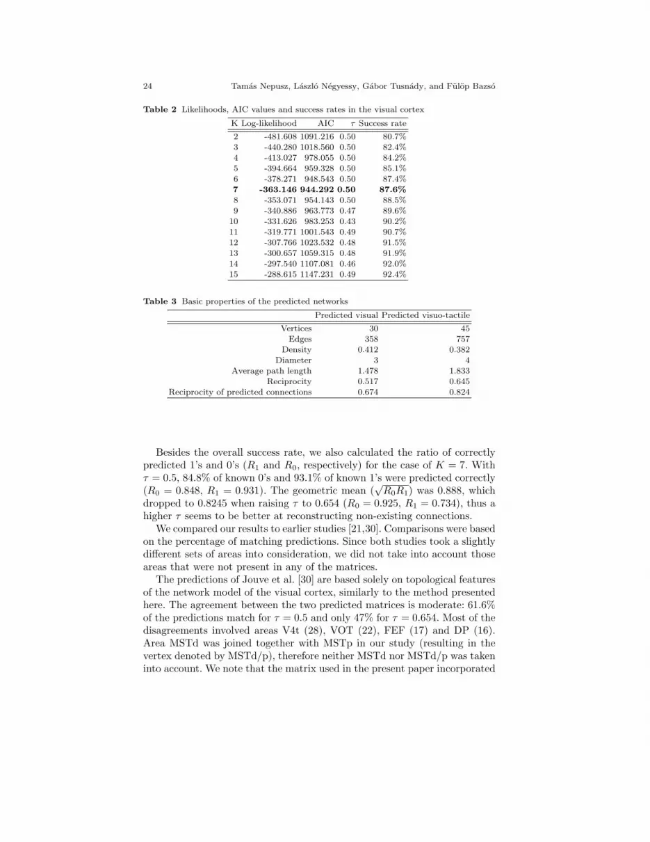
Table 2 Likelihoods, AIC values and success rates in the visual cortex

K Log-likelihood AIC τ Success rate

2 -481.608 1091.216 0.50 80.7%

3 -440.280 1018.560 0.50 82.4%4 -413.027 978.055 0.50 84.2%

5 -394.664 959.328 0.50 85.1%

6 -378.271 948.543 0.50 87.4%7 -363.146 944.292 0.50 87.6%

8 -353.071 954.143 0.50 88.5%

9 -340.886 963.773 0.47 89.6%10 -331.626 983.253 0.43 90.2%

11 -319.771 1001.543 0.49 90.7%12 -307.766 1023.532 0.48 91.5%

13 -300.657 1059.315 0.48 91.9%

14 -297.540 1107.081 0.46 92.0%15 -288.615 1147.231 0.49 92.4%

Table 3 Basic properties of the predicted networks

Predicted visual Predicted visuo-tactile

Vertices 30 45

Edges 358 757Density 0.412 0.382

Diameter 3 4

Average path length 1.478 1.833Reciprocity 0.517 0.645

Reciprocity of predicted connections 0.674 0.824

Besides the overall success rate, we also calculated the ratio of correctlypredicted 1’s and 0’s (R1 and R0, respectively) for the case of K = 7. Withτ = 0.5, 84.8% of known 0’s and 93.1% of known 1’s were predicted correctly(R0 = 0.848, R1 = 0.931). The geometric mean (

√R0R1) was 0.888, which

dropped to 0.8245 when raising τ to 0.654 (R0 = 0.925, R1 = 0.734), thus ahigher τ seems to be better at reconstructing non-existing connections.

We compared our results to earlier studies [21,30]. Comparisons were basedon the percentage of matching predictions. Since both studies took a slightlydifferent sets of areas into consideration, we did not take into account thoseareas that were not present in any of the matrices.

The predictions of Jouve et al. [30] are based solely on topological featuresof the network model of the visual cortex, similarly to the method presentedhere. The agreement between the two predicted matrices is moderate: 61.6%of the predictions match for τ = 0.5 and only 47% for τ = 0.654. Most of thedisagreements involved areas V4t (28), VOT (22), FEF (17) and DP (16).Area MSTd was joined together with MSTp in our study (resulting in thevertex denoted by MSTd/p), therefore neither MSTd nor MSTd/p was takeninto account. We note that the matrix used in the present paper incorporated


V1

V2

V3

V3A

V4

V4t

VOT

VP

MT

MSTd/p

MSTl

PO

LIP

PIP

VIP

DP

7a

FST

PITd

PITv

CITd

CITv

AITd

AITv

STPp

STPa

TF

TH

FEF

46

V1

V2

V3

V3A

V4

V4t

VOT

VP

MT

MSTd/p

MSTl

PO LIP

PIP

VIP

DP

7a FST

PITd

PITv

CITd

CITv

AITd

AITv

STPp

STPa

TF TH FEF

46

0 1 1 1 0 1 0 0 1 0 0 1 0 0 1 0 0 0 0 0 0 0 0 0 0 0 0 0 0 0

1 0 1 1 1 1 0 1 1 1 1 1 1 1 1 1 0 1 0 0 0 0 0 0 0 0 0 0 1 0

1 1 0 1 1 1 0 1 1 1 1 1 1 1 1 1 0 1 0 0 0 0 0 0 0 0 0 0 1 0

1 1 1 0 1 1 0 1 1 1 1 1 1 1 1 1 0 1 0 0 0 0 0 0 0 0 0 0 1 0

1 1 1 1 0 1 1 0 1 0 0 1 0 1 1 0 0 1 1 1 1 1 1 1 1 1 1 1 1 1

1 1 1 1 1 0 0 1 1 1 1 1 1 1 1 1 0 1 0 0 0 0 0 0 0 0 0 0 1 0

0 0 0 0 0 0 0 0 0 0 0 0 0 0 0 0 1 0 0 0 0 0 0 0 1 0 1 0 0 1

1 1 1 1 1 1 0 0 1 1 1 1 1 1 1 1 0 1 0 0 0 0 0 0 0 0 0 0 1 0

1 1 1 1 1 1 0 1 0 1 1 1 1 1 1 1 0 1 0 0 0 0 0 0 0 0 0 0 1 0

0 1 1 1 1 1 1 1 1 0 1 1 1 0 1 1 1 1 0 0 0 0 0 0 1 0 1 0 1 1

0 1 1 1 0 1 0 0 1 0 0 1 0 0 1 0 0 0 0 0 0 0 0 0 0 0 0 0 0 0

1 0 0 0 0 0 0 1 0 1 1 0 1 1 0 1 1 0 0 0 0 0 0 0 0 0 0 0 0 0

0 1 1 1 1 1 1 1 1 1 1 1 0 0 1 1 1 1 0 0 0 0 0 0 1 0 1 0 1 1

1 0 0 0 0 0 0 1 0 1 1 0 1 0 0 1 1 0 0 0 0 0 0 0 0 0 0 0 0 0

0 1 1 1 1 1 1 1 1 1 1 1 1 0 0 1 1 1 0 0 0 0 0 0 1 0 1 0 1 1

1 0 0 0 0 0 0 1 0 1 1 0 1 1 0 0 1 0 0 0 0 0 0 0 0 0 0 0 0 0

0 0 0 0 0 0 1 0 0 0 0 0 0 0 0 0 0 0 0 0 0 0 0 0 1 0 1 0 0 1

0 1 1 1 1 1 1 1 1 1 1 1 1 0 1 1 1 0 0 0 0 0 0 0 1 0 1 0 1 1

0 0 0 0 0 0 1 0 0 0 0 0 0 0 0 0 0 0 0 1 1 1 1 1 1 1 1 1 0 1

0 0 0 0 0 0 1 0 0 0 0 0 0 0 0 0 0 0 1 0 1 1 1 1 1 1 1 1 0 1

0 0 0 0 0 0 1 0 0 0 0 0 0 0 0 0 0 0 1 1 0 1 1 1 1 1 1 1 0 1

0 0 0 0 0 0 1 0 0 0 0 0 0 0 0 0 0 0 1 1 1 0 1 1 1 1 1 1 0 1

0 0 0 0 0 0 1 0 0 0 0 0 0 0 0 0 0 0 1 1 1 1 0 1 1 1 1 1 0 1

0 0 0 0 0 0 1 0 0 0 0 0 0 0 0 0 0 0 1 1 1 1 1 0 1 1 1 1 0 1

0 0 0 0 0 0 1 0 0 0 0 0 0 0 0 0 1 0 0 0 0 0 0 0 0 0 1 0 0 1

0 0 0 0 0 0 1 0 0 0 0 0 0 0 0 0 0 0 1 1 1 1 1 1 1 0 1 1 0 1

0 0 0 0 0 0 1 0 0 0 0 0 0 0 0 0 1 0 0 0 0 0 0 0 1 0 0 0 0 1

0 0 0 0 0 0 1 0 0 0 0 0 0 0 0 0 0 0 1 1 1 1 1 1 1 1 1 0 0 1

0 1 1 1 1 1 1 1 1 1 1 1 1 0 1 1 1 1 0 0 0 0 0 0 1 0 1 0 0 1

0 0 0 0 0 0 1 0 0 0 0 0 0 0 0 0 1 0 0 0 0 0 0 0 1 0 1 0 0 0

Fig. 8 The predicted adjacency matrix of the visual cortex with 7 vertex groups. White

cells denote confirmed existing and absent connections. Dark gray cells denote mismatchesbetween the known and the predicted connectivity. Light gray cells denote predictions for

unknown connections.

the results of anatomical experiments that could not have been included inthe matrix in [30], therefore the moderate match between the two matricescan be explained by the differences in the initial dataset, see Table 4 forthe number of mismatches involving each area. Since the prediction methodof Jouve et al. was not concerned with reconstructing the entire network(predictions were made only on unknown connections), no comparison couldbe made based on the success rates of the two methods.

The predictions published by Costa et al. [21] are based on several topo-logical (e.g., node degree, clustering coefficient) and spatial features (e.g.,area sizes, local density of the areas in the 3D space, based on their knownpositions in the cortex). In this sense, the reconstruction method based onthe preference model is simpler, for it depends solely on the connection ma-


Table 4 Number of mismatches in the predicted matrix, grouped by areas

Known connections Jouve et al. [30] Costa et al. [21]

V1 5 0 0

V2 5 1 0V3 6 0 0

V3A 1 4 1

V4 21 0 0V4t 2 28 15

VOT 7 22 18

VP 10 0 –MT 3 2 0

MSTd/p 5 – –MSTl 7 7 0

PO 10 3 1

LIP 8 3 3PIP 5 13 4

VIP 4 6 3

DP 12 16 87a 9 10 7

FST 11 8 1

PITd 6 6 2PITv 4 7 6

CITd 2 9 3

CITv 3 8 5AITd 7 2 1

AITv 4 8 3STPp 11 9 8

STPa 6 12 3

TF 13 8 11TH 6 8 2

FEF 8 17 3

46 15 7 9

In the second column, the known connections of the original matrix are compared toour predictions. In the last two columns, only the unknown (predicted) connections are

compared to the unknown connections of our dataset. The 4 largest number of mismatches

in each column are underlined.

trix. We also note that Costa et al. inferred the topological features from asymmetrized connectivity matrix, thus their predicted matrix is also com-pletely symmetric, while our method produced a matrix where only 67.4%of the connections (67.4% of the predicted, previously unknown connections)were reciprocal. The ratios of correctly predicted 1’s and 0’s in the visualcortex reported by Costa et al. were slightly worse (R0 = 244/350 = 0.697,R1 = 207/295 = 0.701,

√R0R1 = 0.699, loop connections excluded). Note

that the comparison can not be fully accurate because of the slightly differentset of areas used in the analysis (MIP and MDP were present only in [21],whereas MSTd/p and VP were present only in the matrix used in this study).69.8% of the predictions presented here matched the predictions of [21], and


all predicted edges with a probability larger than 0.8 were predicted in [21]as well.

One may note that in spite of the improvement of the reconstruction ascompared to the previous studies [21,30], there is still a relatively high num-ber of mismatches on Fig. 8. The distribution of mismatches in the adjacencymatrix can be suggestive of the methodological shortcomings and the stateof knowledge in the investigated network. It appears that most of the mis-matches are to be found within the two major visual clusters, the dorsal andventral visual subsystems, where connectional densities are higher than inthe lower left and upper right quadrants of the matrix representing the inter-cluster connections. Interestingly, most of the mismatches affected either theinput or output patterns of areas V4 and 46, and to a lesser degree of TF andFEF in the intercluster regions. These areas are central nodes in the visualcortical network, establishing connections between different clusters. In fact,the inclusion of the sensorimotor cortex improved the reconstruction (seeSection 3.4). It is also noteworthy that relatively few mismatches/violationsoccurred in case of the lower order areas (listed in the upper left corner of thematrix). This is an important point as low-level areas establish connectionsmostly within their cluster and the connections of these areas are relativelywell explored. These observations indicate the dependence of reconstructionquality on the actual knowledge of the network.

To summarize without going into the details, we conclude that our re-construction is biologically realistic and reflects our understanding of theorganization of the visual cortical connectivity.

3.4 Visuo-tactile cortex

The network model of the visuo-tactile cortex is an extension of the visualcortex, obtained by adding the 15 areas of the sensorimotor cortex and theirrespective connections. Connections going between a visual and a sensorimo-tor area are called heteromodal connections. The density of the sensorimotorcortex is slightly higher than that of the visual cortex. Based on the con-nection densities, the probability of the existence of an unknown connectionwas assumed to be 0.385 inside the visual cortex and 0.404 inside the sen-sorimotor cortex. Unknown heteromodal connections were assumed to existwith probability 0.1. Note that the vast majority of heteromodal connectionsis unknown. There was no confirmed nonexisting sensorimotor connectionindicated in the data set. The adjacency matrix is shown on Fig. 5. The opti-mal configuration was found by combining the greedy optimization with theMCMC method, similarly as above.

The number of groups in the preference model was determined again bythe Akaike information criterion. The eigenvalues of the Laplacian and thesingular values of the adjacency matrix suggested 5 groups, which is again in


Table 5 Likelihoods, AIC values and success rates in the visuo-tactile cortex

K Log-likelihood AIC τ Success rate

5 -814.956 1859.913 0.42 83.6%

6 -783.935 1819.871 0.23 84.4%7 -756.352 1790.705 0.46 84.8%

8 -736.163 1780.327 0.37 86.1%

9 -718.422 1778.844 0.43 86.4%10 -697.078 1774.156 0.49 87.3%

11 -683.335 1788.671 0.46 89.3%

12 -684.105 1836.210 0.46 89.3%13 -665.337 1848.674 0.47 89.4%

14 -653.755 1879.510 0.48 89.4%15 -652.173 1934.347 0.40 90.1%

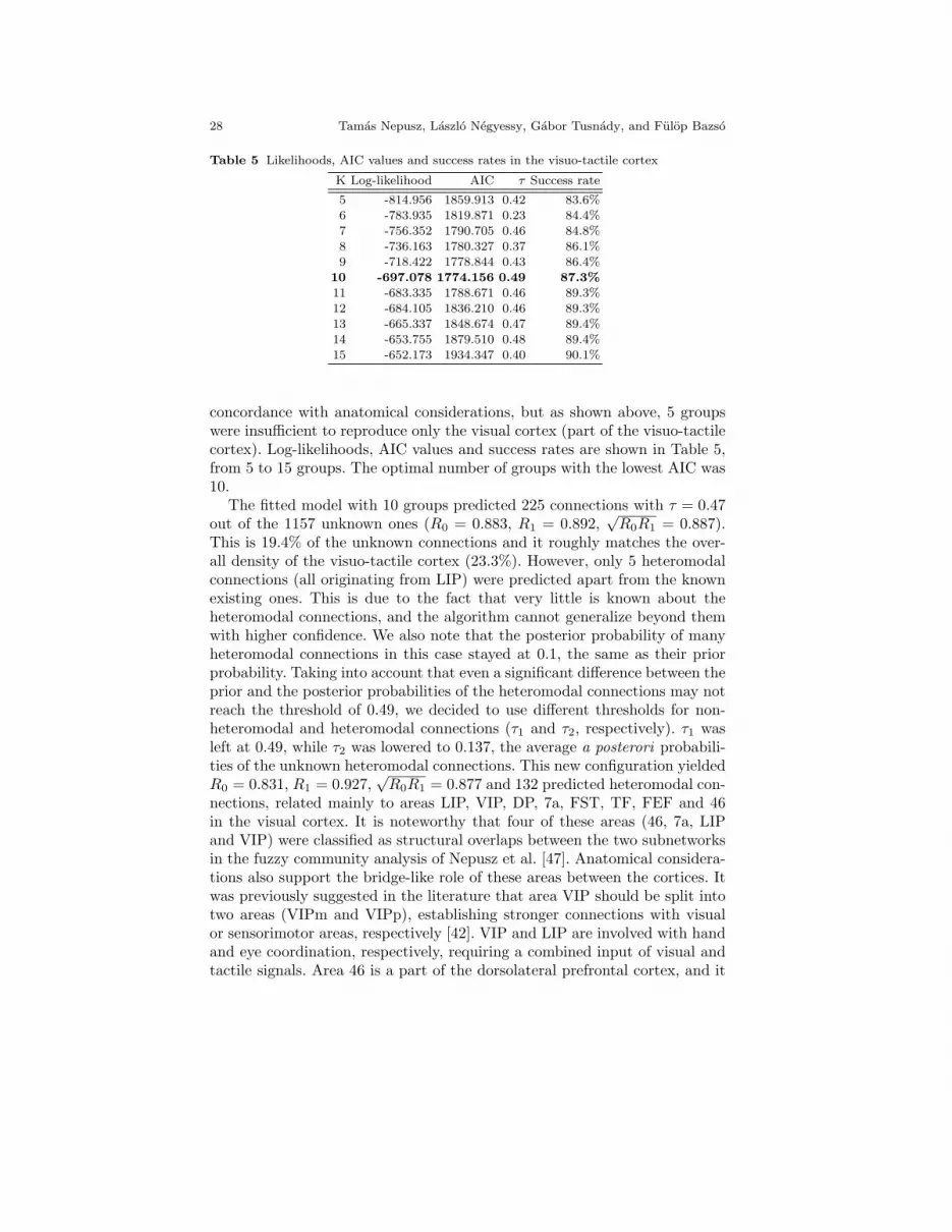
concordance with anatomical considerations, but as shown above, 5 groupswere insufficient to reproduce only the visual cortex (part of the visuo-tactilecortex). Log-likelihoods, AIC values and success rates are shown in Table 5,from 5 to 15 groups. The optimal number of groups with the lowest AIC was10.

The fitted model with 10 groups predicted 225 connections with τ = 0.47out of the 1157 unknown ones (R0 = 0.883, R1 = 0.892,

√R0R1 = 0.887).

This is 19.4% of the unknown connections and it roughly matches the over-all density of the visuo-tactile cortex (23.3%). However, only 5 heteromodalconnections (all originating from LIP) were predicted apart from the knownexisting ones. This is due to the fact that very little is known about theheteromodal connections, and the algorithm cannot generalize beyond themwith higher confidence. We also note that the posterior probability of manyheteromodal connections in this case stayed at 0.1, the same as their priorprobability. Taking into account that even a significant difference between theprior and the posterior probabilities of the heteromodal connections may notreach the threshold of 0.49, we decided to use different thresholds for non-heteromodal and heteromodal connections (τ1 and τ2, respectively). τ1 wasleft at 0.49, while τ2 was lowered to 0.137, the average a posterori probabili-ties of the unknown heteromodal connections. This new configuration yieldedR0 = 0.831, R1 = 0.927,

√R0R1 = 0.877 and 132 predicted heteromodal con-

nections, related mainly to areas LIP, VIP, DP, 7a, FST, TF, FEF and 46in the visual cortex. It is noteworthy that four of these areas (46, 7a, LIPand VIP) were classified as structural overlaps between the two subnetworksin the fuzzy community analysis of Nepusz et al. [47]. Anatomical considera-tions also support the bridge-like role of these areas between the cortices. Itwas previously suggested in the literature that area VIP should be split intotwo areas (VIPm and VIPp), establishing stronger connections with visualor sensorimotor areas, respectively [42]. VIP and LIP are involved with handand eye coordination, respectively, requiring a combined input of visual andtactile signals. Area 46 is a part of the dorsolateral prefrontal cortex, and it


Table 6 Group affiliations of the areas in the visuo-tactile cortex

Out-group 1 V1, VOT, MSTlOut-group 2 V2, V3, V3A, V4t, VP, MT, PO, PIP

Out-group 3 V4

Out-group 4 MSTd/p, FST, FEFOut-group 5 LIP, VIP

Out-group 6 DP, 7a

Out-group 7 PITd, PITv, CITd, CITv, AITd, AITv, STPp, STPa, THOut-group 8 TF, 46

Out-group 9 3a, 1, 2, 5, SII, 7b, 4, 6, SMA

Out-group 10 3b, Ri, Ig, Id, 35, 36

In-group 1 V1, PIPIn-group 2 V2, V3, V3A, V4t, VP, MT, PO

In-group 3 35, 36

In-group 4 V4, FST, FEFIn-group 5 VIP

In-group 6 MSTd/p, MSTl, LIP, DP, 7a

In-group 7 PITd, PITv, CITd, CITv, AITd, AITv, STPp, STPa, THIn-group 8 VOT, TF, 46

In-group 9 3a, 1, 2, 5, SII, 7b, 4, 6, SMA

In-group 10 3b, Ri, Ig, Id

does not have functions related to low-level sensory information processing.Being a higher level (supramodal) area, it integrates visual, tactile and otherinformation. Area 7a integrates visual, tactile and proprioceptive signals. Fi-nally, areas TF and FEF are also high level structures integrating widespreadcortical information (e.g., [20]).

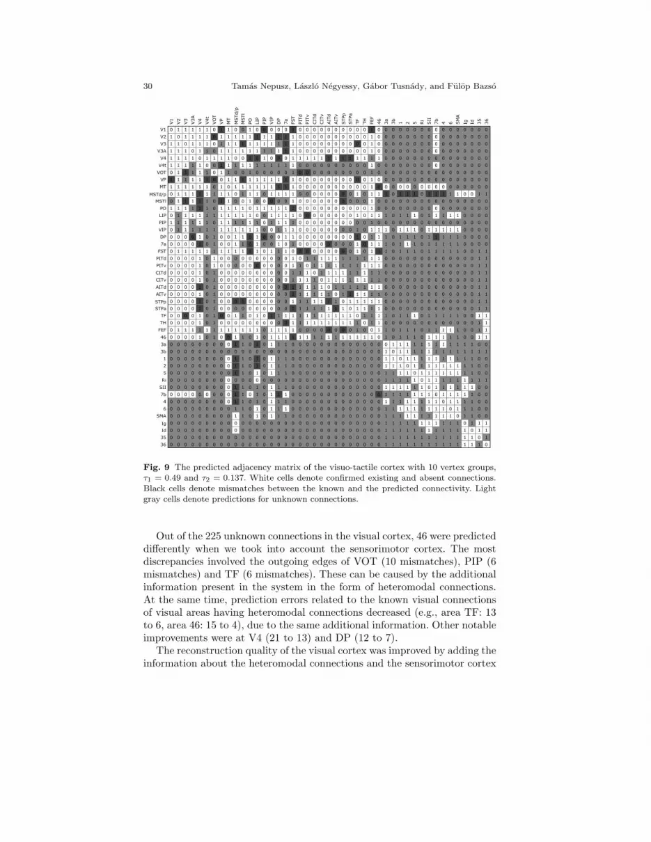
The predicted connectivity matrix is shown on Fig. 9, the basic graphmeasures are depicted in Table 3. To show the subtle differences betweenpredicted connections, the exact probabilities are shown on Fig. 10, encodedin the background colour of the matrix cells (white indicating zero probabilityand black indicating 1). The latter figure shows the prediction in its fulldetail, especially in the sensorimotor cortex where the predicted clique-likesubgraph reveals its internal structure more precisely. The group affiliationsof the individual vertices are shown in Table 6.

We also examined the ratios of correctly predicted known 0’s and 1’swith respect to pure visual and pure sensorimotor connections. As expected,the algorithm performed better in the visual cortex, which is more thor-ougly charted than the sensorimotor cortex. The calculated ratios wereR0 = 0.865, R1 = 0.902,

√R0R1 = 0.882 for the visual cortex. Since the

sensorimotor cortex contained no known non-existing connections, R1 couldnot be calculated for it. All known connections in the sensorimotor cortexwere predicted correctly (R0 = 1), however, this is due to the lack of infor-mation on nonexisting connections in the sensorimotor cortex. The ratios ofthe visual cortex were similar to the ones obtained when analyzing the visualcortex alone.


V1

V2

V3V3AV4

V4t

VOTVPMT

MSTd/pMSTlPOLIPPIPVIPDP

7a

FST

PITdPITv

CITdCITv

AITdAITv

STPpSTPa

TFTHFEF

463a

3b1

25Ri

SII

7b4

6SMA

IgId3536

V1

V2

V3

V3A

V4

V4t

VOT

VP

MT

MSTd/p

MSTl

PO LIP

PIP

VIP

DP

7a FST

PITd

PITv

CITd

CITv

AITd

AITv

STPp

STPa

TF TH FEF

46 3a 3b 1 2 5 Ri

SII

7b 4 6 SMA

Ig Id 35 36

0 1 1 1 1 1 0 1 1 0 0 1 0 0 0 0 0 1 0 0 0 0 0 0 0 0 0 0 1 0 0 0 0 0 0 0 0 0 0 0 0 0 0 0 01 0 1 1 1 1 0 1 1 1 1 1 1 1 1 1 1 1 0 0 0 0 0 0 0 0 0 0 1 0 0 0 0 0 0 0 0 0 0 0 0 0 0 0 01 1 0 1 1 1 0 1 1 1 1 1 1 1 1 1 1 1 0 0 0 0 0 0 0 0 0 0 1 0 0 0 0 0 0 0 0 0 0 0 0 0 0 0 01 1 1 0 1 1 0 1 1 1 1 1 1 1 1 1 1 1 0 0 0 0 0 0 0 0 0 0 1 0 0 0 0 0 0 0 0 0 0 0 0 0 0 0 01 1 1 1 0 1 1 1 1 0 0 1 0 1 0 0 0 1 1 1 1 1 1 1 1 1 1 1 1 1 0 0 0 0 0 0 0 0 0 0 0 0 0 0 01 1 1 1 1 0 0 1 1 1 1 1 1 1 1 1 1 1 0 0 0 0 0 0 0 0 0 0 1 0 0 0 0 0 0 0 0 0 0 0 0 0 0 0 00 1 1 1 1 1 0 1 1 0 0 1 0 0 0 0 0 1 0 0 0 0 0 0 0 0 0 0 1 0 0 0 0 0 0 0 0 0 0 0 0 0 0 0 01 1 1 1 1 1 0 0 1 1 1 1 1 1 1 1 1 1 0 0 0 0 0 0 0 0 0 0 1 0 0 0 0 0 0 0 0 0 0 0 0 0 0 0 01 1 1 1 1 1 0 1 0 1 1 1 1 1 1 1 1 1 0 0 0 0 0 0 0 0 0 0 1 0 0 0 0 0 0 0 0 0 0 0 0 0 0 0 00 1 1 1 1 1 1 1 1 0 1 1 1 0 1 1 1 1 0 0 0 0 0 0 0 0 1 0 1 1 1 0 1 1 1 0 1 1 1 1 1 0 0 1 1

0 1 1 1 1 1 0 1 1 0 0 1 0 0 0 0 0 1 0 0 0 0 0 0 0 0 0 0 1 0 0 0 0 0 0 0 0 0 0 0 0 0 0 0 01 1 1 1 1 1 0 1 1 1 1 0 1 1 1 1 1 1 0 0 0 0 0 0 0 0 0 0 1 0 0 0 0 0 0 0 0 0 0 0 0 0 0 0 00 1 1 1 1 1 1 1 1 1 1 1 0 0 1 1 1 1 0 0 0 0 0 0 0 0 1 0 1 1 1 0 1 1 1 0 1 1 1 1 1 0 0 0 01 1 1 1 1 1 0 1 1 1 1 1 1 0 1 1 1 1 0 0 0 0 0 0 0 0 0 0 1 0 0 0 0 0 0 0 0 0 0 0 0 0 0 0 00 1 1 1 1 1 1 1 1 1 1 1 1 0 0 1 1 1 0 0 0 0 0 0 0 0 1 0 1 1 1 0 1 1 1 0 1 1 1 1 1 0 0 0 00 0 0 0 1 0 1 0 0 1 1 0 1 0 0 0 1 1 0 0 0 0 0 0 0 0 1 0 1 1 1 0 1 1 1 0 1 1 1 1 1 0 0 0 00 0 0 0 1 0 1 0 0 1 1 0 1 0 0 1 0 1 0 0 0 0 0 0 0 0 1 0 1 1 1 0 1 1 1 0 1 1 1 1 1 0 0 0 00 1 1 1 1 1 1 1 1 1 1 1 1 0 1 1 1 0 0 0 0 0 0 0 0 0 1 0 1 1 1 0 1 1 1 0 1 1 1 1 1 0 0 1 1

0 0 0 0 1 0 1 0 0 0 0 0 0 0 0 0 0 1 0 1 1 1 1 1 1 1 1 1 1 1 0 0 0 0 0 0 0 0 0 0 0 0 0 1 1

0 0 0 0 1 0 1 0 0 0 0 0 0 0 0 0 0 1 1 0 1 1 1 1 1 1 1 1 1 1 0 0 0 0 0 0 0 0 0 0 0 0 0 1 1

0 0 0 0 1 0 1 0 0 0 0 0 0 0 0 0 0 1 1 1 0 1 1 1 1 1 1 1 1 1 0 0 0 0 0 0 0 0 0 0 0 0 0 1 1

0 0 0 0 1 0 1 0 0 0 0 0 0 0 0 0 0 1 1 1 1 0 1 1 1 1 1 1 1 1 0 0 0 0 0 0 0 0 0 0 0 0 0 1 1

0 0 0 0 1 0 1 0 0 0 0 0 0 0 0 0 0 1 1 1 1 1 0 1 1 1 1 1 1 1 0 0 0 0 0 0 0 0 0 0 0 0 0 1 1

0 0 0 0 1 0 1 0 0 0 0 0 0 0 0 0 0 1 1 1 1 1 1 0 1 1 1 1 1 1 0 0 0 0 0 0 0 0 0 0 0 0 0 1 1

0 0 0 0 1 0 1 0 0 0 0 0 0 0 0 0 0 1 1 1 1 1 1 1 0 1 1 1 1 1 0 0 0 0 0 0 0 0 0 0 0 0 0 1 1

0 0 0 0 1 0 1 0 0 0 0 0 0 0 0 0 0 1 1 1 1 1 1 1 1 0 1 1 1 1 0 0 0 0 0 0 0 0 0 0 0 0 0 1 1

0 0 0 0 1 0 1 0 0 1 1 0 1 0 1 1 1 1 1 1 1 1 1 1 1 1 0 1 1 1 1 0 1 1 1 0 1 1 1 1 1 0 0 1 1

0 0 0 0 1 0 1 0 0 0 0 0 0 0 0 0 0 1 1 1 1 1 1 1 1 1 1 0 1 1 0 0 0 0 0 0 0 0 0 0 0 0 0 1 1

0 1 1 1 1 1 1 1 1 1 1 1 1 0 1 1 1 1 0 0 0 0 0 0 0 0 1 0 0 1 1 0 1 1 1 0 1 1 1 1 1 0 0 1 1

0 0 0 0 1 0 1 0 0 1 1 0 1 0 1 1 1 1 1 1 1 1 1 1 1 1 1 1 1 0 1 0 1 1 1 0 1 1 1 1 1 0 0 1 1

0 0 0 0 0 0 0 0 0 1 1 0 1 0 1 1 1 0 0 0 0 0 0 0 0 0 0 0 0 0 0 1 1 1 1 1 1 1 1 1 1 1 1 0 00 0 0 0 0 0 0 0 0 0 0 0 0 0 0 0 0 0 0 0 0 0 0 0 0 0 0 0 0 0 1 0 1 1 1 1 1 1 1 1 1 1 1 1 1

0 0 0 0 0 0 0 0 0 1 1 0 1 0 1 1 1 0 0 0 0 0 0 0 0 0 0 0 0 0 1 1 0 1 1 1 1 1 1 1 1 1 1 0 00 0 0 0 0 0 0 0 0 1 1 0 1 0 1 1 1 0 0 0 0 0 0 0 0 0 0 0 0 0 1 1 1 0 1 1 1 1 1 1 1 1 1 0 00 0 0 0 0 0 0 0 0 1 1 0 1 0 1 1 1 0 0 0 0 0 0 0 0 0 0 0 0 0 1 1 1 1 0 1 1 1 1 1 1 1 1 0 00 0 0 0 0 0 0 0 0 0 0 0 0 0 0 0 0 0 0 0 0 0 0 0 0 0 0 0 0 0 1 1 1 1 1 0 1 1 1 1 1 1 1 1 1

0 0 0 0 0 0 0 0 0 1 1 0 1 0 1 1 1 0 0 0 0 0 0 0 0 0 0 0 0 0 1 1 1 1 1 1 0 1 1 1 1 1 1 0 00 0 0 0 0 0 0 0 0 1 1 0 1 0 1 1 1 0 0 0 0 0 0 0 0 0 0 0 0 0 1 1 1 1 1 1 1 0 1 1 1 1 1 0 00 0 0 0 0 0 0 0 0 1 1 0 1 0 1 1 1 0 0 0 0 0 0 0 0 0 0 0 0 0 1 1 1 1 1 1 1 1 0 1 1 1 1 0 00 0 0 0 0 0 0 0 0 1 1 0 1 0 1 1 1 0 0 0 0 0 0 0 0 0 0 0 0 0 1 1 1 1 1 1 1 1 1 0 1 1 1 0 00 0 0 0 0 0 0 0 0 1 1 0 1 0 1 1 1 0 0 0 0 0 0 0 0 0 0 0 0 0 1 1 1 1 1 1 1 1 1 1 0 1 1 0 00 0 0 0 0 0 0 0 0 0 0 0 0 0 0 0 0 0 0 0 0 0 0 0 0 0 0 0 0 0 1 1 1 1 1 1 1 1 1 1 1 0 1 1 1

0 0 0 0 0 0 0 0 0 0 0 0 0 0 0 0 0 0 0 0 0 0 0 0 0 0 0 0 0 0 1 1 1 1 1 1 1 1 1 1 1 1 0 1 1

0 0 0 0 0 0 0 0 0 0 0 0 0 0 0 0 0 0 0 0 0 0 0 0 0 0 0 0 0 0 1 1 1 1 1 1 1 1 1 1 1 1 1 0 1

0 0 0 0 0 0 0 0 0 0 0 0 0 0 0 0 0 0 0 0 0 0 0 0 0 0 0 0 0 0 1 1 1 1 1 1 1 1 1 1 1 1 1 1 0

Fig. 9 The predicted adjacency matrix of the visuo-tactile cortex with 10 vertex groups,τ1 = 0.49 and τ2 = 0.137. White cells denote confirmed existing and absent connections.

Black cells denote mismatches between the known and the predicted connectivity. Light

gray cells denote predictions for unknown connections.

Out of the 225 unknown connections in the visual cortex, 46 were predicteddifferently when we took into account the sensorimotor cortex. The mostdiscrepancies involved the outgoing edges of VOT (10 mismatches), PIP (6mismatches) and TF (6 mismatches). These can be caused by the additionalinformation present in the system in the form of heteromodal connections.At the same time, prediction errors related to the known visual connectionsof visual areas having heteromodal connections decreased (e.g., area TF: 13to 6, area 46: 15 to 4), due to the same additional information. Other notableimprovements were at V4 (21 to 13) and DP (12 to 7).

The reconstruction quality of the visual cortex was improved by adding theinformation about the heteromodal connections and the sensorimotor cortex


Fig. 10 Probability of the connections in the visuo-tactile cortex with 10 vertex groups,τ1 = 0.49 and τ2 = 0.137. Probabilities are denoted by colours, with white corresponding

to 0 and black corresponding to 1. The predicted adjacency matrix is shown in the matrix

cells.

(see Fig. 8 and the upper left part of Fig. 9). This was not a simple conse-quence of increasing the number of clusters from 7 to 10, but the corollary ofthe additional information about the connections that visual areas form withthe sensorimotor cortex. This contextual information may also give guidelinesfor understanding the mechanisms of heteromodal interactions.

3.5 Major structural changes after reconstruction

An interesting feature of the reconstructed network is the complete cliqueinduced by the following vertices: PITd, PITv, CITd, CITv, AITd, AITv,STPp, STPa, TF and TH. We note that this region was mostly uncharted


in the original matrix, and there were only three confirmed nonexisting con-nections (STPp → AITd and STPa ↔ AITv). This clique also appeared inthe earlier analysis of Jouve et al. [30] and a similar but smaller clique alsoemerged in our predictions of the visual cortex. Notably, a similar tendencycould also be observed in the analysis of Costa et al. [21], as only a few con-nections were missing among the areas mentioned above to form a clique.Our assumption is that our prediction based on solely the visual cortex is amore accurate approximation of the true connectional pattern of these areas.

Finally, we compared the community structure of the original and the pre-dicted connectivity matrix in order to obtain further support for the validityof our predictions. We argue that a valid predicted connectivity matrix shouldnot only obtain a high ratio of correctly predicted 1’s and 0’s, but also keepthe community structure of the network mostly intact. In order to take thedirectionality of the edges into account, we employed the community detec-tion method of Latapy & Pons [40]. This method is based on the idea thatgiven a significant community structure in the network, short random walkstend to stay within the same community. We tried random walks with lengthranging from 3 to 7. The quality of the obtained partitions was assessedby the modularity function Q [48]. Best results were achieved with randomwalks of length 7 for the original and 4 for the predicted cortex (Q = 0.339and Q = 0.301, respectively). Table 7 shows the detected communities of theoriginal and the predicted visuo-tactile cortex.

Table 7 Community structure of the original and the predicted visuo-tactile cortex

Original visuo-tactile cortex (Q = 0.339)

Community 1 V1, V2, V3, V3A, V4t, VP, MT, MSTd/p, MSTl, PO, LIP, PIP,VIP, DP, 7a, FST, FEF, 46

Community 2 V4, VOT, PITd, PITv, CITd, CITv, AITd, AITv, STPp, STPa,

TF, THCommunity 3 3a, 3b, 1, 2, 5, Ri, SII, 7b, 4, 6, SMA

Community 4 Ig, Id, 35, 36

Predicted visuo-tactile cortex (Q = 0.379)

Community 1 V1, V2, V3, V3A, V4t, VP, MT, MSTd/p, MSTl, PO, LIP, PIP,

VIP, DP, 7a, FST, FEF, 46Community 2 V4, VOT, PITd, PITv, CITd, CITv, AITd, AITv, STPp, STPa,

TF, THCommunity 3 3a, 3b, 1, 2, 5, Ri, SII, 7b, 4, 6, SMA, Ig, Id, 35, 36

Community 1 corresponds approximately to the dorsal stream of the visualcortex while community 2 contains the areas of the ventral stream in bothcases. Community 3 and community 4 form the sensorimotor cortex. Thesegroups were joined together to form a single community of the sensorimotorcortex in the case of the predicted matrix. Since there is no known anatomicalmeaning of community 4, the predicted community structure represents ourunderstanding of the sensorimotor cortex more accurately than the originalone. Apart from this mismatch, we can conclude that the major structure of


the original matrix was preserved during the reconstruction process, but thereconstructed network seems less modular than the original, as indicated bythe decrease in the modularity of the partitions.

Other notable differences were the smaller diameter and shorter averagepath length (Table 1, 3). Considering segregation and integration as majorcortical functions [66], these findings together predict a more efficient corticalinformation processing as it can be deduced on the basis of our present stateof knowledge about this network.

4 Conclusion

From a biological point of view, the stochastic representation of the corti-cal network described in the present study demonstrates the high level ofuncertainty of our knowledge about the connectivity of the ventral visualcluster (community 2) as well as the sensorimotor cortex (communities 3 and4). Similarly to our findings, both previous studies [21, 30] predicted numer-ous connections within the ventral visual cluster, making it almost a large,fully connected clique. A similar observation was made here in the sensori-motor cortex. We should note that in contrast to the dorsal visual cluster(including the majority of areas in community 1) there is a massive lackof information regarding the non-existence of the connections in the ventraland sensorimotor clusters (see also [20]). Considering the deterministicallyimperfect knowledge of the cortical, and probably most of the real-life com-plex networks, these findings point out the significance of information aboutknown nonexistent connections. Interestingly, similar conclusion was drawnby Kotter and Stephan [38], who investigated the role of components in cor-tical information processing by defining their network participation indices.This is an important point when considering that neurobiologists focus onthe existence of connections between the cortical areas and often ignore theabsence of them while mapping cortical connections in their experiments.In fact, this point is in agreement with our expectations considering thatthe cortical network architecture is shaped by evolutionary and functionalconstraints.

Considering individual cortical areas, our predictions resulted in a rela-tively large number of mismatches of the connections of some mid- (e.g., V4and DP) and high level areas (e.g., TF and 46) when compared to the orig-inal data. The connections of high level areas, which form the connectionsbetween the different cortical clusters, are hard to predict in individual sub-networks where the connections between these areas and the neglected partof the network is necessarily missing from the data. The largest number ofmismatches occurred in the case of V4. This area is a functionally hetero-geneous, complex structure, which maybe divided to sub-regions, and formsa bridge between the dorsal and ventral clusters of the visual cortex [47].


This could at least partly explain the large number of mismatches occurredin the reconstruction process. The assumption outlined here is further sup-ported by the fact that the number of mismatches involving areas V4, DP,TF and 46 decreased after taking into account the sensorimotor cluster andthe heteromodal connections. On the other hand, V4t and VOT are exam-ples of structures with largely unexplored connectivity. The existing datasuggest that these areas exhibit roughly similar pattern of connectivity totheir topographical neighbor area V4, which has much better explored con-nectivity. The large differences observed in the predicted connectivity of V4tand VOT in the three studies (including ours as well as Costa et al. [21] andJouve et al. [30]) is most probably due to the large uncertainty in the con-nectional data of these two areas. Interestingly, a more careful examinationof Fig. 8 suggest that the prediction of the connections of these three areas,especially that of V4 and VOT tended to be somewhat complementary inthe visual cortex. This was less evident in the larger visuo-tactile network(Fig. 9). Based on these observations it is suggested that the mismatches ofV4-connections occurred during the reconstruction as a consequence of theoptimization process.

From the methodological point of view it is important to note that our ap-proach is not a community structure detection. There are many sophisticatedmethods which reliably detect communities within networks [17, 40, 48, 53],yet the information about the community structure is not sufficient for anaccurate network reconstruction. One of the main advantages of our methodis a higher accuracy in reconstruction of charted connections (known existentor nonexistent), compared to earlier methods [21,30]. It is important to em-phasize that our method allows the prediction of nonreciprocal connections.The presented approach is general and applicable to other networks not nec-essarily related to cortical structure. Its generality is reflected in the fact thatwe do not use information about the underlying spatial structure, as thesedata may be unavailable or unintelligible for some networks, nor we assumethat there is a given property of paths related to the clustering coefficient inthe network. Our method is based on an exact goal function that we optimize.The existence of a goal function allows for a comparison of different solutionswhich may be difficult to carry out in the absence of a quantitative measure.The drawbacks of our approach are related to the necessity of knowledgeregarding existing and confirmed nonexisting connections. This necessity isreflected in the prediction of heteromodal connections, as the number of con-firmed or refuted heteromodal connections is surprisingly small, see Fig. 5.One has to note that the method is computationally expensive, which maybe a severe limiting factor in case of large networks. Finally, inspired by theSzemeredi regularity lemma, the present study exemplifies the usefulness ofa theoretical approach in analyzing real world data.


Acknowledgments

Laszlo Negyessy acknowledges the support of the Janos Bolyai ResearchScholarship of the Hungarian Academy of Sciences.

References

1. Achard, S., Bullmore, E.: Efficiency and cost of economical brain functional networks.

PLoS Comp Biol 3(2), e17 (2007)2. Akaike, H.: A new look at the statistical model identification. IEEE Trans Automat

Contr 19(6), 716–723 (1974)

3. Andrieu, C., de Freitas, N., Doucet, A., Jordan, M.I.: An introduction to MCMC formachine learning. Mach Learn 50, 5–43 (2003)

4. Angelucci, A., Bullier, J.: Reaching beyond the classical receptive field of V1 neurons:

horizontal or feedback axons? J Physiol 97(2-3), 141–54 (2003)5. Arbib, M.A., Erdi, P.: Precis of Neural organization: structure, function and dynamics.

Behav Brain Sci 23(4), 513–33 (2000). Discussion: pp. 533-716. Bienenstock, E.: On the dimensionality of cortical graphs. J Physiol 90(3-4), 251–6

(1996)

7. Braitenberg, V., Schuz, A.: Cortex: Statistics and Geometry of Neuronal Connectivity.Springer (1998)

8. Bressler, S.L., Tognoli, E.: Operational principles of neurocognitive networks. Int J

Psychophysiol 60(2), 139–48 (2006)9. Buzas, P., Kovacs, K., Ferecsko, A.S., Budd, J.M., Eysel, U.T., Kisvarday, Z.F.: Model-

based analysis of excitatory lateral connections in the visual cortex. J Comp Neurol

499(6), 861–81 (2006)10. Buzsaki, G., Geisler, C., Henze, D.A., Wang, X.J.: Interneuron diversity series: Circuit

complexity and axon wiring economy of cortical interneurons. Trends Neurosci 27(4),

186–93 (2004)11. Calvin, W.H.: Cortical columns, modules, and Hebbian cell assemblies. In: M.A. Ar-

bib (ed.) Handbook of Brain Theory and Neural Networks, pp. 269–272. BradfordBooks/MIT Press (1995)

12. Chung, F.R.K.: Laplacians and the Cheeger inequality for directed graphs. Ann Com-

binator 9, 1–19 (2005)13. Clauset, A., Moore, C., Newman, M.E.J.: Structural inference of hierarchies in net-

works. In: Proceedings of the 23rd International Conference on Machine Learning

(ICML) (2006)14. Csardi, G., Nepusz, T.: The igraph software package for complex network research.

InterJournal Complex Systems p. 1695 (2006)

15. Danon, L., Duch, J., Diaz-Guilera, A., Arenas, A.: Comparing community structureidentification. J Stat Mech p. P09008 (2005)

16. DeFelipe, J., Alonso-Nanclares, L., Arellano, J.I.: Microstructure of the neocortex:

comparative aspects. J Neurocytol 31(3-5), 299–316 (2002)17. van Dongen, S.: A stochastic uncoupling process for graphs. Tech. Rep. INS-R0011,

National Research Institute for Mathematics and Computer Science in the Netherlands(2000)

18. Douglas, R.J., Martin, K.A.: Mapping the matrix: the ways of neocortex. Neuron

56(2), 226–38 (2007)19. Edelman, G.M.: Neural Darwinism: selection and reentrant signaling in higher brain

function. Neuron 10(2), 115–25 (1993)


20. Felleman, D.J., Van Essen, D.C.: Distributed hierarchical processing in the primate

cerebral cortex. Cerebr Cortex 1(1), 1–47 (1991)21. da Fontoura Costa, L., Kaiser, M., Hilgetag, C.C.: Predicting the connectivity of pri-

mate cortical networks from topological and spatial node properties. BMC Syst Biol

1(16) (2007)22. Fred, A.L.N., Jain, A.K.: Robust data clustering. In: Proceedings of the IEEE Com-

puter Society Conference on Computer Vision and Pattern Recognition, vol. 2, pp.

128–133. IEEE (2003). DOI 10.1109/CVPR.2003.121146223. Freeman, W.J.: Mesoscopic neurodynamics: from neuron to brain. J Physiol 94(5-6),

303–22 (2000)24. Geman, S., Geman, D.: Stochastic relaxation, Gibbs distributions and the Bayesian

restoration of images. IEEE Trans Pattern Anal Mach Intell 6, 721–741 (1984)

25. Hastings, W.K.: Monte Carlo sampling methods using Markov chains and their appli-cations. Biometrika 57(1), 97–109 (1970). DOI 10.2307/2334940

26. Hilgetag, C.C., Burns, G.A., O’Neill, M.A., Scannell, J.W., Young, M.P.: Anatomi-

cal connectivity defines the organization of clusters of cortical areas in the macaquemonkey and the cat. Philos Trans R Soc Lond B Biol Sci 355(1393), 91–110 (2000)

27. Hilgetag, C.C., Grant, S.: Uniformity, specificity and variability of corticocortical con-

nectivity. Philos Trans R Soc Lond B Biol Sci 355(1393), 7–20 (2000)28. Hilgetag, C.C., O’Neill, M.A., Young, M.P.: Hierarchical organization of macaque and

cat cortical sensory systems explored with a novel network processor. Philos Trans R

Soc Lond B Biol Sci 355(1393), 71–89 (2000)29. Ioannides, A.A.: Dynamic functional connectivity. Curr Opin Neurobiol 17, 161–70

(2007)30. Jouve, B., Rosenstiehl, P., Imbert, M.: A mathematical approach to the connectivity

between the cortical visual areas of the macaque monkey. Cerebr Cortex 8(1), 28–39

(1998)31. Kaas, J.H.: Organizing principles of sensory representations. Novartis Foundation

symposium 228, 188–198 (2000)

32. Kaiser, M.: Brain architecture: a design for natural computation. Philos Transact AMath Phys Eng Sci 365(1861), 3033–45 (2007)

33. Kaiser, M., Hilgetag, C.C.: Modelling the development of cortical systems networks.

Neurocomputing 58-60, 297–302 (2004)34. Kaiser, M., Hilgetag, C.C.: Nonoptimal component placement, but short processing

paths, due to long-distance projections in neural systems. PLoS Comp Biol 2(7), e95

(2006)35. Kisvarday, Z.F., Ferecsko, A.S., Kovacs, K., Buzas, P., M., B.J., Eysel, U.T.: One

axon-multiple functions: specificity of lateral inhibitory connections by large basketcells. J Neurocytol 31(3-5), 255–64 (2002)

36. Komlos, J., Simonovits, M.: Szemeredi’s regularity lemma and its applications in graph

theory. In: D. Miklos, V.T. Sos, T. Szonyi (eds.) Combinatorics, Paul Erdos is Eighty,Vol. 2, pp. 295–352. Janos Bolyai Mathematical Society, Budapest (1996)

37. Kotter, R.: Online retrieval, processing, and visualization of primate connectivity data

from the cocomac database. Neuroinformatics 2, 127–144 (2004)38. Kotter, R., Stephan, K.E.: Network participation indices: characterizing component

roles for information processing in neural networks. Neural Network 16(9), 1261–75(2003)

39. Kullback, S., Leibler, R.A.: On information and sufficiency. Ann Math Stat 22, 79–86

(1951)

40. Latapy, M., Pons, P.: Computing communities in large networks using random walks.J Graph Algorithm Appl 10(2), 191–218 (2006)

41. Lee, L., Friston, K., Horwitz, B.: Large-scale neural models and dynamic causal mod-elling. NeuroImage 30, 1243–54 (2006)


42. Lewis, J.W., Van Essen, D.C.: Corticocortical connections of visual, sensorimotor and

multimodal processing areas in the parietal lobe of the macaque monkey. J CompNeurol 428, 112–137 (2000)

43. Montenegro, R., Tetali, P.: Mathematical aspects of mixing times in Markov chains.

Foundations and Trends in Theoretical Computer Science 1(3), 237–354 (2006). DOI10.1561/0400000003

44. Mountcastle, V.B.: The columnar organization of the neocortex. Brain 120(4), 701–22(1997)

45. Negyessy, L., Nepusz, T., Kocsis, L., Bazso, F.: Prediction of the main cortical areas

and connections involved in the tactile fuction of the visual cortex by network analysis.Eur J Neurosci 23(2), 1919–1930 (2006)

46. Negyessy, L., Nepusz, T., Zalanyi, L., Bazso, F.: Convergence and divergence are

mostly reciprocated properties of the connections in the network of cortical areas.Proc Roy Soc B 275(1649), 2403–2410 (2008). DOI 10.1098/rspb.2008.0629

47. Nepusz, T., Petroczi, A., Negyessy, L., Bazso, F.: Fuzzy communities and the concept

of bridgeness in complex networks. Phys Rev E 77, 016,107 (2008)48. Newman, M.E.J.: Modularity and community structure in networks. Proc Natl Acad

Sci Unit States Am 103(23), 8577–8582 (2006)49. Newman, M.E.J., Leicht, E.A.: Mixture models and exploratory analysis in networks.

Proc Natl Acad Sci Unit States Am 104(23), 9564–9569 (2007). DOI 10.1073/pnas.

061053710450. Passingham, R.E., Stephan, K.E., Kotter, R.: The anatomical basis of functional lo-

calization in the cortex. Nat Rev Neurosci 3(8), 606–16 (2002)51. Petroni, F., Panzeri, S., Hilgetag, C.C., Kotter, R., Young, M.P.: Simultaneity of re-

sponses in a hierarchical visual network. NeuroReport 12(12), 2753–9 (2001)52. http://www.ncbi.nlm.nih.gov/PubMed/

53. Reichardt, J., Bornholdt, S.: Detecting fuzzy community structures in complex net-works with a Potts model. Phys Rev Lett 93, 218,701 (2004)

54. Rockland, K.S.: Non-uniformity of extrinsic connections and columnar organization.

J Neurocytol 31(3-5), 247–53 (2002)55. Rockland, K.S., N., I.: Some thoughts on cortical minicolumns. Exp Brain Res 158(3),

256–77 (2004)56. Roe, A.W.: Modular complexity of area V2 in the macaque monkey. In: C. Collins,

J. Kaas (eds.) The Primate Visual System, pp. 109–138. CRC Press (2003)57. Roe, A.W., Ts’o, D.Y.: Specificity of color connectivity between primate V1 and V2.

J Neurophysiol 82(5), 2719–30 (1999)58. Sporns, O.: Graph theory methods for the analysis of neural connectivity patterns. In:

R. Kotter (ed.) Neuroscience Databases. A Practical Guide. Kluwer (2002)59. Sporns, O., Chialvo, D.R., Kaiser, M., Hilgetag, C.C.: Organization, development and

function of complex brain networks. Trends Cognit Sci 8(9), 418–25 (2004)60. Sporns, O., Honey, C.J., Kotter, R.: Identification and classification of hubs in brain

networks. PLoS ONE 2(10), e1049 (2007)61. Stettler, D.D., Das, A., Bennett, J., Gilbert, C.D.: Lateral connectivity and contextual

interactions in macaque primary visual cortex. Neuron 36(4), 739–50 (2002)62. Szemeredi, E.: Regular partitions of graphs. In: E. du Centre National de la Recherche

Scientifique (CNRS) (ed.) Problemes combinatoires et theorie des graphes (Colloq.Internat. CNRS, Univ. Orsay, Orsay, 1976, pp. 399–401. Paris (1978)

63. Szentagothai, J.: The “module-concept” in cerebral cortex architecture. Brain Res95(2-3), 475–96 (1975)

64. Szentagothai, J.: Specificity versus (quasi-) randomness revisited. Acta Morphologica

Hungarica 38, 159–167 (1990)65. Tao, T.: Szemeredi’s regularity lemma revisited. Contributions to Discrete Mathemat-

ics 1, 8–28 (2006)66. Tononi, G., Edelman, G.M., Sporns, O.: Complexity and coherency: integrating infor-

mation in the brain. Trends Cognit Sci 2, 474–84 (1998)


67. Van Essen, D.C., Dierker, D.L.: Surface-based and probabilistic atlases of primate

cerebral cortex. Neuron 56, 209–25 (2007)68. Young, M.P.: Objective analysis of the topological organization of the primate cortical

visual system. Nature 358(6382), 152–5 (1992)

69. Zhu, M., Ghodsi, A.: Automatic dimensionality selection from the scree plot via theuse of profile likelihood. Computational Statistics and Data Analysis 51(2), 918–930

(2006). DOI 10.1016/j.csda.2005.09.010

Index

Akaike information criterion, 12

bridge vertex, 33

cerebral cortex, 2CoCoMac, 3, 19

cognitive functions, 3

connectional similarity, 3cortical areas, 3

dorsal visual, 33

sensorimotor, 33ventral visual, 33

cortical column, 2

directedness, 3

experimental data, 3

Gibbs sampling, 11

graph modelpreference, 4

stochastic, 4graph partitioning, 5

greedy optimization, 8

integration

neural, 2

Kullback-Leibler divergence, 13

likelihood, 7log-likelihood, see likelihood

macaque monkey, 3

Markov chain Monte Carlo method, 9

matrixadjacency, 12

directed Laplacian, 12

Laplacian, 12

maximum likelihood estimation, 8membership vector, 7

Metropolis-Hastings algorithm, 10

networksstochastic reconstruction, 3

stochastic representation, 33

neural connectionsheteromodal, 33

indirect, 21

long distance, 2nonexistent, 34

nonreciprocal, 34neuron doctrine, 2

neuronal diversity, 2

optimization

goal function, 34stochastic, 34

overfitting, 9, 12

Perron vector, 12Perron-Frobenius theorem, 12

quasi-randomness, 2

reciprocity, 3

segregationneural, 2

singular value decomposition, 12synapse, 2

SzemerediEndre Szemeredi, 5regularity lemma, 5

uncertainty, 3

39

Reconstructing Cortical Networks: Case of Directed Graphs with High Level of Reciprocity

Documents