Journal of Marine Research, 70, 569–602, 2012 Reconciling float-based and tracer-based estimates of lateral diffusivities by Andreas Klocker 1,2 , Raffaele Ferrari 1 , Joseph H. LaCasce 3 and Sophia T. Merrifield 1 ABSTRACT Lateral diffusivities are computed from synthetic particles and tracers advected by a velocity field derived from sea-surface height measurements from the South Pacific, in a region west of Drake Passage. Three different estimates are compared: (1) the tracer-based “effective diffusivity” of Nakamura (1996), (2) the growth of the second moment of a cloud of tracer and (3) the single- and two-particle Lagrangian diffusivities. The effective diffusivity measures the cross-stream component of eddy mixing, so this article focuses on the meridional diffusivities for the others, as the mean flow (the ACC) is zonally oriented in the region. After an initial transient of a few weeks, the effective diffusivity agrees well with the meridional diffusivity estimated both from the tracer cloud and from the particles. This proves that particle- and tracer-based estimates of eddy diffusivities are equivalent, despite recent claims to the contrary. Convergence among the three estimates requires that the Lagrangian diffusivities be estimated using their asymptotic values, not their maximum values. The former are generally much lower than the latter in the presence of a mean flow. Sampling the long-time asymptotic behavior of Lagrangian diffusivities requires very large numbers of floats in field campaigns. For example, it is shown that hundreds of floats would be necessary to estimate the vertical and horizontal variations in eddy diffusivity in a sector of the Pacific Southern Ocean. 1. Introduction Quantifying tracer transport by geostrophic eddies is one of the outstanding problems in large-scale ocean dynamics. Geostrophic eddies set the rate at which tracers like heat and carbon are mixed laterally and vertically in the ocean and play a central role in determining large-scale circulation patterns, such as the meridional overturning circulation (see, e.g., the reviews by Olbers et al., 2004; Marshall and Speer, 2012). The mixing induced by geostrophic eddies is often quantified in terms of an eddy diffu- sivity. The component of the diffusivity across the mean currents is most relevant, because 1. Department of Earth, Atmospheric, and Planetary Sciences, Massachusetts Institute of Technology, Cambridge, Massachusetts, 02139, U.S.A. 2. Corresponding author. email: [email protected] 3. Department of Geosciences, University of Oslo, Norway. 569

Welcome message from author
This document is posted to help you gain knowledge. Please leave a comment to let me know what you think about it! Share it to your friends and learn new things together.
Transcript
Journal of Marine Research, 70, 569–602, 2012
Reconciling float-based and tracer-based estimates oflateral diffusivities
by Andreas Klocker1,2, Raffaele Ferrari1, Joseph H. LaCasce3 andSophia T. Merrifield1
ABSTRACTLateral diffusivities are computed from synthetic particles and tracers advected by a velocity
field derived from sea-surface height measurements from the South Pacific, in a region west ofDrake Passage. Three different estimates are compared: (1) the tracer-based “effective diffusivity” ofNakamura (1996), (2) the growth of the second moment of a cloud of tracer and (3) the single- andtwo-particle Lagrangian diffusivities. The effective diffusivity measures the cross-stream componentof eddy mixing, so this article focuses on the meridional diffusivities for the others, as the mean flow(the ACC) is zonally oriented in the region.
After an initial transient of a few weeks, the effective diffusivity agrees well with the meridionaldiffusivity estimated both from the tracer cloud and from the particles. This proves that particle-and tracer-based estimates of eddy diffusivities are equivalent, despite recent claims to the contrary.Convergence among the three estimates requires that the Lagrangian diffusivities be estimated usingtheir asymptotic values, not their maximum values. The former are generally much lower than thelatter in the presence of a mean flow.
Sampling the long-time asymptotic behavior of Lagrangian diffusivities requires very large numbersof floats in field campaigns. For example, it is shown that hundreds of floats would be necessary toestimate the vertical and horizontal variations in eddy diffusivity in a sector of the Pacific SouthernOcean.
1. Introduction
Quantifying tracer transport by geostrophic eddies is one of the outstanding problems inlarge-scale ocean dynamics. Geostrophic eddies set the rate at which tracers like heat andcarbon are mixed laterally and vertically in the ocean and play a central role in determininglarge-scale circulation patterns, such as the meridional overturning circulation (see, e.g.,the reviews by Olbers et al., 2004; Marshall and Speer, 2012).
The mixing induced by geostrophic eddies is often quantified in terms of an eddy diffu-sivity. The component of the diffusivity across the mean currents is most relevant, because
1. Department of Earth, Atmospheric, and Planetary Sciences, Massachusetts Institute of Technology,Cambridge, Massachusetts, 02139, U.S.A.
2. Corresponding author. email: [email protected]. Department of Geosciences, University of Oslo, Norway.
569
570 Journal of Marine Research [70, 4
tracer transport along currents is generally dominated by the current itself. The cross-currenteddy diffusivity K is defined as
v′C ′ = −KCy, (1)
where v′C ′ is the cross-current tracer flux and Cy is the cross-current tracer gradient.4
Overbars denote large-scale averages and primes are departures from those averages. Asnoted hereafter, there are discrepancies in the literature about both the magnitude and spatialpatterns of K , and it is a goal of this paper to help resolve these discrepancies.
Estimates of K can be obtained from Eulerian data, from tracer distributions and fromLagrangian (particle) data. Early attempts to estimateK with Eulerian data relied on mooringtime series of velocity v and tracer C (e.g., temperature) to construct v′C ′ and its relationshipto Cy (e.g., Bryden and Heath, 1985). However, the time series are often too short for sig-nificant results (Wunsch, 1999). In addition, the estimates are hampered by the presence oflarge, nondivergent eddy fluxes that do not contribute to mixing (Marshall and Shutts, 1981).
Another example of Eulerian estimates is the use of satellite measurements of sea-surfaceheight (SSH) in conjunction with mixing length theory (Prandtl, 1925) to estimate diffusivi-ties, as proposed by Holloway (1986) and Ferrari and Nikurashin (2010). This approach hasthe advantage that time series at fixed locations lend themselves well to the determination ofmean and residual quantities. The weakness is that the eddy diffusivity can be determinedup to undetermined constants that appear in the mixing length theory.
Tracer-based estimates can be made from hydrographic data. Armi and Stommel (1983)studied the oxygen distribution in the Eastern North Atlantic in the context of an advective-diffusive equation and inferred an eddy diffusivity of approximately 500 m2s−1 at 800 mdepth. Similarly, Ferrari (2005) and Zika et al. (2010) used temperature and salinity obser-vations in the same region to estimate diffusivities of O(1000 m2s−1) at the surface andO(100 m2s−1) below 1,500 m. Jenkins (1998) studied tritium and 3He distributions in thesame ocean patch and estimated K ∼ 1,200 m2s−1 at a depth of 300 m.
Such estimates assume a steady state of advection and diffusion. The evolution of theeddy diffusivity can only be deduced with observations of a time-evolving tracer distribution,as in the North Atlantic Tracer Release Experiment (NATRE; Ledwell et al., 1998). Thediffusivity can then be estimated from the dispersion of the patch. The NATRE release (ofsulphur hexafluoride) yielded an estimate of K ∼ 1,000 m2s−1 at 300 m depth, consistentwith the steady-state estimates of Jenkins (1998).
Lagrangian estimates on the other hand derive from the trajectories of freely driftinginstruments, like surface drifters and subsurface floats (e.g., Davis, 1991; LaCasce, 2008).The diffusivity is proportional to the derivative of the mean square separation of the particles
4. In general one expects the tracer flux to have both a down gradient and a skew component, v′C′ = −KCy +KskewCx . Here we assume that the averaging is taken over a long sector of the current so that Cx ≈ 0 and theskew component can be ignored. In the simulations described below Cx is identically zero, because we imposeperiodic boundary conditions to the tracer advected in the numerical channel.
2012] Klocker et al.: Reconciling estimates of lateral diffusivities 571
from their starting positions, as first proposed by Taylor (1921). Early diffusivity estimatesfrom drifting buoys in the North Atlantic were made by Freeland et al. (1975), Colin deVerdiere (1983) and Krauss and Böning (1987). Colin de Verdiere (1983) obtained a merid-ional diffusivity of K ∼ 1,700 m2s−1 at the surface and Freeland et al. (1975) obtainedK ∼ 700 m2s−1 at 1,500 m depth.
However, some subsequent estimates were much larger. Zhurbas and Oh (2004) obtainedvalues in excess of 4,000 m2s−1 at the surface in the Western Atlantic, reaching values of20,000 m2s−1 in the vicinity of the Gulf Stream. Lumpkin et al. (2002) and McClean et al.(2002) found comparable values.
Diffusivities have also been measured in the Southern Ocean, which is the focus of thispaper, and here too the results vary. Eulerian-based estimates, from SSH, yield values of2,000–4,000 m2s−1 in the Antarctic Circumpolar Current (ACC), with smaller values in thesubtropical gyres to the north (Keffer and Holloway, 1988; Stammer, 1998). However thetracer-based estimates differ. Using a technique proposed by Nakamura (1996) (Section 2),Marshall et al. (2006) obtained values of O(1,000 m2s−1) near the core of the ACC andlarger values of O(2,000 m2s−1) to the north. This method yields only the cross-streamcomponent of the diffusivity and thus in principle does not suffer from “contamination” bythe mean flow or by skew fluxes. Lower diffusivities in the ACC are consistent with themean flow suppressing cross-stream mixing (e.g., Ferrari and Nikurashin, 2010). The ACCweakens with depth, suggesting the diffusivity should have a subsurface maximum (as theeddy field is intensified near the current). Abernathey et al. (2010) found this to be the case,using the tracer-based diagnostic.
Lagrangian estimates, in contrast, tend to be larger. Lumpkin and Pazos (2007) and Salléeet al. (2008) obtained values in the vicinity of the ACC of approximately 4,000 m2s−1, usingsurface drifters, with smaller values north and south of the jet. The exception was near thewestern boundary currents, where the diffusivities were large. Consistent with some earlierstudies in the North Atlantic (e.g., Lumpkin et al., 2002, and references therein), Salléeet al. (2008) found that K is correlated with the eddy kinetic energy; the largest values werenear the ACC, where eddy variability is most pronounced. However, not all the Lagrangianestimates agree. Using synthetic float data from a numerical model, Griesel et al. (2010)found much smaller cross-stream diffusivities, O(750 m2s−1), in the polar frontal zone,consistent with the tracer-derived estimates. However, they did not observe a suppressionof eddy mixing in the ACC itself, nor did their diffusivities exhibit a subsurface maximum.
Thus there are discrepancies among the estimates particularly in the Southern Ocean.This is a significant challenge for ocean and climate simulations, because coarse-resolutionmodels are sensitive to the magnitude and the lateral and vertical structures of eddy diffusiv-ities in the Southern Ocean (Griffies et al., 2005; Danabasoglu and Marshall, 2007). Indeed,ocean models can reproduce reasonable stratification and transports with meridional eddydiffusivities in the range of a few hundred to one thousand m2s−1 (e.g., Griffies et al., 2005).As such, it is important to understand why the tracer, Eulerian and Lagrangian diffusivityestimates differ.
572 Journal of Marine Research [70, 4
Several studies have addressed this question previously. Sundermeyer and Price (1998)used an idealized ocean model to reproduce eddy statistics from the NATRE field campaigndescribed above and simulated the motion of synthetic floats and tracers. Their Lagrangianestimates of K were two to six times larger than the tracer-based estimates. Riha andEden (2011) used an idealized zonally periodic channel with eddy-driven zonal jets tocompare Lagrangian and Eulerian diffusivity estimates. Interestingly, their estimates werecomparable, with the Lagrangian ones being slightly smaller. Incidentally, both methodsindicated an increase of the eddy diffusivities with depth.
In the present work, we examine further the relationship between different diffusivity esti-mates. To this end, we use a three-dimensional velocity field representative of the SouthernOcean, derived from satellite measurements of SSH, to estimate eddy diffusivities from trac-ers and floats. We focus on a region in the Southern Ocean upstream from Drake passage,which is the site of a large field experiment, the Diapycnal and Isopycnal Mixing Experi-ment in the Southern Ocean (DIMES). A major goal of DIMES is to infer eddy diffusivitiesfrom tracer and float releases. Here we focus on diffusivity estimates; in a companion paper(Klocker et al., 2012), we examine mixing suppression by the mean flow.
The results suggest that cross-stream estimates of eddy diffusivities from both Lagrangianstatistics and tracer releases converge if measured properly and if the statistics are adequate.The comparison is hindered by the mean flow, which causes the Lagrangian diffusivity toovershoot its asymptotic value. Correct estimates thus require integrating past this overshoot.
The paper is organized as follows: Section 2 examines the different methods for calcu-lating the diffusivity and how they are related; Section 3 describes how we construct thevelocity field used to advect tracers and floats; and Section 4 presents and compares thediffusivity estimates for a sector of the Southern Ocean upstream of Drake Passage. Section5 then uses these results to discuss the implications for observational estimates of eddydiffusivities. The results are discussed in Section 6.
2. Theory
Here we compare theoretical estimates of tracer-based and particle-based diffusivities.The former is described by Nakamura (1996), Shuckburgh and Haynes (2003) and Marshallet al. (2006). The term derives from the advection-diffusion equation for a passive tracer,C(x, y, t):
∂
∂tC + ∇ · (uC) = ∇ · (κ∇C), (2)
where u is taken to be a two-dimensional (horizontal) velocity, assumed nondivergent, andκ is a small-scale diffusivity. The latter might be the molecular diffusivity or a numericaldiffusivity imposed to make solutions stable. The equation can be written as a simplediffusion equation when expressed in coordinates defined by the tracer isolines
∂
∂tC = ∂
∂A
(Knak
∂C
∂A
), (3)
2012] Klocker et al.: Reconciling estimates of lateral diffusivities 573
where A is the area bounded by an isoline of the tracer C, assumed to be a monotonicfunction of C. Further,
Knak = κ
(∂C/∂A)2
∂
∂A
∫∫|∇C|2 dA (4)
is Nakamura’s effective diffusivity. This is proportional to the small-scale diffusivity, κ,but it also depends on the gradient of C, integrated over the area bounded by the isoline.Thus if stirring acts to increase the gradients, the effective diffusivity can be much largerthan the small-scale value. Note that Knak has units of (length)2/time, in contrast to a usualdiffusivity.
Nakamura’s effective diffusivity is often written in terms of a ratio of squared lengthscales:
Ke ≥ Kel ≡ kL2
L20
(5)
and we introduced the lower bound of the effective diffusivity Kel. Leq is an equivalentlength greater than or equal to L, the length of the tracer contour (Shuckburgh and Haynes2003); L0 is the initial length of the contour; and Ke = Knak/L
20. This form shows that the
effective diffusivity exceeds the small-scale value if the tracer contour is elongated by theadvecting flow:
Ke ≥= κL2
L20
, (6)
During the initial straining, before small-scale mixing sets in, the area between tracer con-tours is approximately conserved (as the flow is non-divergent), and one can estimate L
equivalently from tracers and particles (which do not experience mixing).We can use the relationship in (6) to make the connection with the Lagrangian diffusivities.
We think of the tracer contour as being made up of N discrete particles. Then the squaredlength of the contour is given by
L2 =N−1∑n=1
(rn+1 − rn)2 =
N−1∑n=1
(xn+1 − xn)2 + (yn+1 − yn)
2, (7)
where rn = (xn, yn) is the position of the n-th particle. Clearly:
L2 = N < �r2 >, (8)
where < �r2 > is the mean square spacing between the particles. This is the relativedispersion of particle pairs (e.g., Bennett, 2006). Thus if the area between tracer isolines isconserved, we have
Kel = κ< �r2 >
< �r20 >
. (9)
So the lower bound effective diffusivity is proportional to the relative dispersion.
574 Journal of Marine Research [70, 4
But how is the effective diffusivity related to the particle diffusivity? Following Taylor(1921), the Lagrangian diffusivity is given by:
K1 = 1
2
d
dt< (r − r0)
2 >, (10)
where r is the position of a particle, r0 is its initial position and the brackets indicate anaverage over all particles. This applies to single particles, and accordingly we refer to (10)as the single-particle diffusivity. However, one can also define a relative diffusivity (ortwo-particle diffusivity):
K2 = 1
4
d
dt< �r2 > (11)
(e.g., Batchelor and Townsend, 1956; Davis, 1985; Babiano et al., 1990). The factor of 1/4is arbitrary but useful, as described below. An important point is that the relative diffusivity,unlike the single-particle diffusivity, is Galilean invariant.
Now if the stirring is nonlocal (dominated by larger-scale eddies), the relative dispersionincreases exponentially with time (Lin, 1972; Bennett, 1984; Babiano et al., 1990; LaCasce,2008):
< �r2 > = < �r20 > et/τ, (12)
where τ is a time scale, usually determined by the root mean squared shear. From (9),the effective diffusivity will also grow exponentially with time, with the same e-foldingtime scale, τ. With exponential growth, the relative diffusivity is proportional to the relativedispersion (11). So the lower bound of the effective and relative diffusivities are proportionalto one another
Kel = κ4τK2
〈�r20 〉 . (13)
But this equivalence follows from two assumptions: first, that the area is conservedbetween tracer contours and second, that the stirring is nonlocal. The relation will pre-sumably break down if either assumption is violated. So, for example, the diffusivitiesshould differ under local stirring, as occurs in a two-dimensional inverse-energy cascade orthree-dimensional forward-energy cascade (e.g., LaCasce, 2008).
In numerical studies, the effective diffusivity asymptotes to a constant value when thesmall-scale diffusion is actively mixing away the tracer gradients (Nakamura, 2008). Areais no longer conserved between isolines, implying the lower bound in (6) is no longer useful.The relative dispersion, on the other hand, continues to grow. When particle separations arelarge enough, the pair velocities are uncorrelated and the relative diffusivity, defined withthe prefactor of one-fourth, asymptotes to the single-particle diffusivity, K2 → K1 (e.g.,Babiano et al., 1990; LaCasce, 2008). At this point, relative dispersion grows linearly intime, as for a diffusive process. But as the effective diffusivity is constant, the two cannot bethe same at later times (see (9) for the relation between the effective diffusivity and relativedispersion).
The Lagrangian diffusivities (the time derivative of dispersion) should also asymptote toconstant values at later times, provided there are no long-term correlations in the velocities
2012] Klocker et al.: Reconciling estimates of lateral diffusivities 575
(Taylor, 1921). Yet there is no guarantee that the particle diffusivities will agree with thetracer-derived estimate. Indeed, the former derive purely from advective considerationswhile the latter are based on an areal integration, which effectively removes the advectiveterm from the tracer equation. While the effective diffusivity is proportional to the small-scale diffusivity, the relative diffusivity is determined essentially by the scale and kineticenergy of the energy-containing eddies. The two diffusivities are expected to converge, ifthe rate at which tracers are homogenized is set by the large-scale eddies and not by small-scale diffusion. This probably happens in strongly turbulent fields where the large-scaleeddies set the rate at which tracer filaments are generated. Once generated, the filamentsare stretched and folded until they are homogenized by small-scale diffusion. A reductionof small-scale diffusion does not alter the rate of tracer homogenization, rather it results inthinner filaments that can be irreversibly mixed faster to keep up with the rate of filamentgeneration.
Previous results suggest that the two diffusivities are the same, at least for some ide-alized flows. A collection of particles constitutes a tracer, and thus an initial distributionshould evolve according to the same diffusion equation (3). Shuckburgh and Haynes (2003)examined this, computing numerical solutions to this equation, using the effective diffu-sivity diagnosed from a simple analytical flow field, and comparing the solutions to time-evolving distributions of particles advected by the same flow. The close agreement suggeststhat particles effectively obey the same diffusion equation. So the diffusivity measured bythe particles and the tracer ought to agree.
We test this hereafter using numerical calculations of evolving tracer fields and particledistributions using a velocity field representative of the Southern Ocean.
3. The velocity field
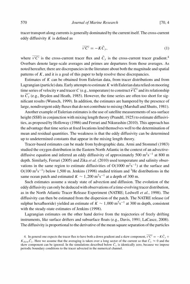
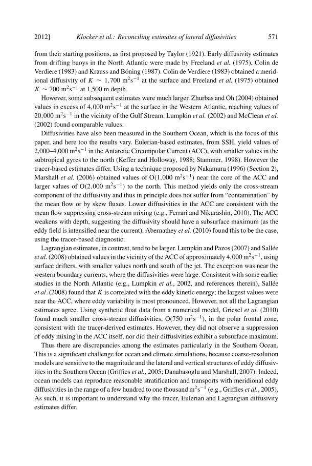
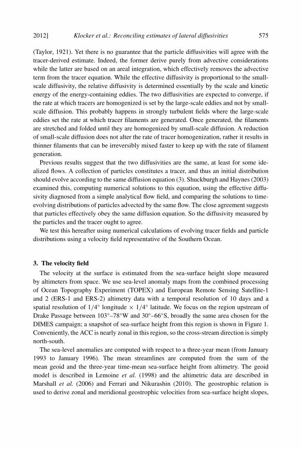
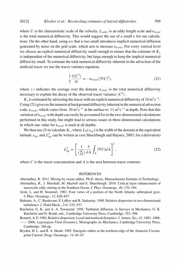
The velocity at the surface is estimated from the sea-surface height slope measuredby altimeters from space. We use sea-level anomaly maps from the combined processingof Ocean Topography Experiment (TOPEX) and European Remote Sensing Satellite-1and 2 (ERS-1 and ERS-2) altimetry data with a temporal resolution of 10 days and aspatial resolution of 1/4◦ longitude × 1/4◦ latitude. We focus on the region upstream ofDrake Passage between 103◦–78◦W and 30◦–66◦S, broadly the same area chosen for theDIMES campaign; a snapshot of sea-surface height from this region is shown in Figure 1.Conveniently, the ACC is nearly zonal in this region, so the cross-stream direction is simplynorth-south.
The sea-level anomalies are computed with respect to a three-year mean (from January1993 to January 1996). The mean streamlines are computed from the sum of themean geoid and the three-year time-mean sea-surface height from altimetry. The geoidmodel is described in Lemoine et al. (1998) and the altimetric data are described inMarshall et al. (2006) and Ferrari and Nikurashin (2010). The geostrophic relation isused to derive zonal and meridional geostrophic velocities from sea-surface height slopes,
576 Journal of Marine Research [70, 4
Figure 1. Snapshot of sea-surface height (m) as estimated from the combined processing of theTOPEX, ERS-1 and ERS-2 altimetries for an ACC sector upstream of Drake Passage between103◦–78◦W and 30◦–66◦S.
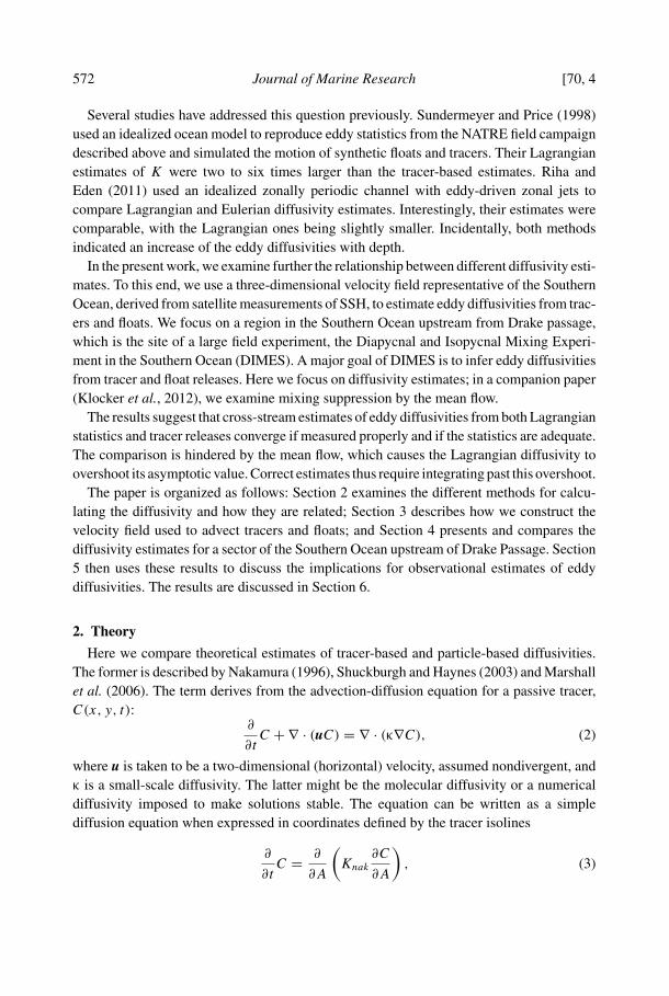
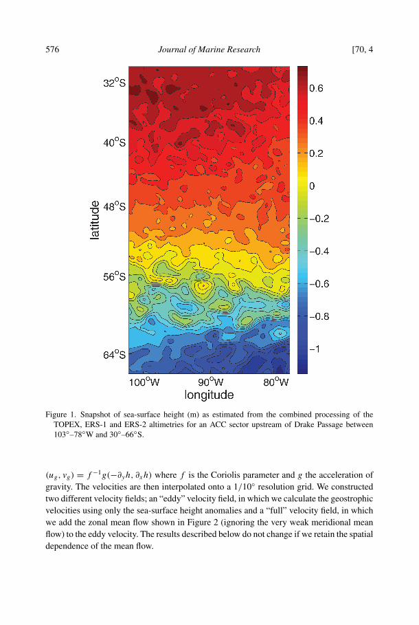
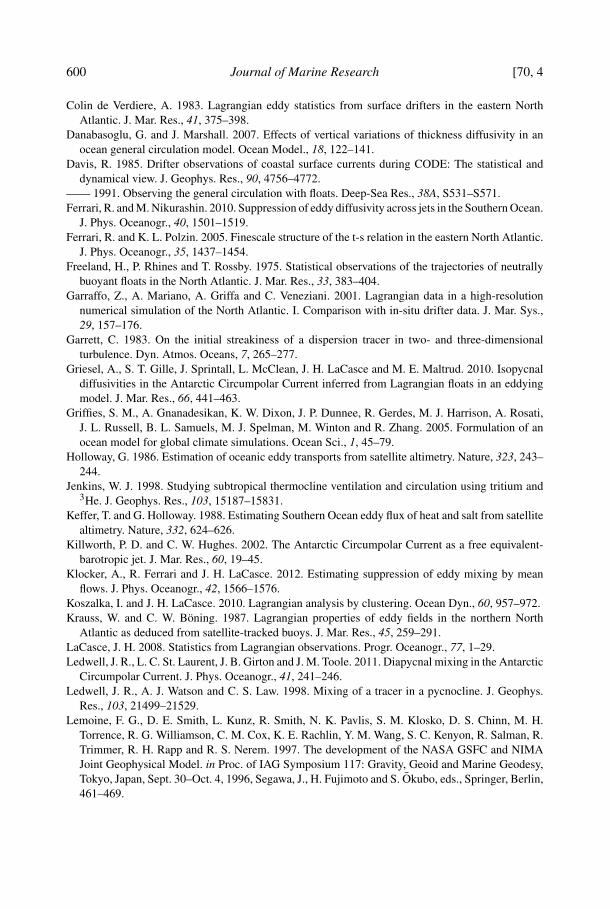
(ug, vg) = f −1g(−∂yh, ∂xh) where f is the Coriolis parameter and g the acceleration ofgravity. The velocities are then interpolated onto a 1/10◦ resolution grid. We constructedtwo different velocity fields; an “eddy” velocity field, in which we calculate the geostrophicvelocities using only the sea-surface height anomalies and a “full” velocity field, in whichwe add the zonal mean flow shown in Figure 2 (ignoring the very weak meridional meanflow) to the eddy velocity. The results described below do not change if we retain the spatialdependence of the mean flow.
2012] Klocker et al.: Reconciling estimates of lateral diffusivities 577
Figure 2. Zonal mean and three-year time mean (from January 1993 to January 1996) surface velocityfor the domain shown in Figure 1.
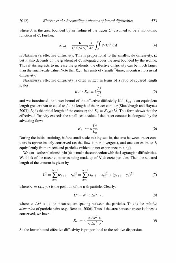
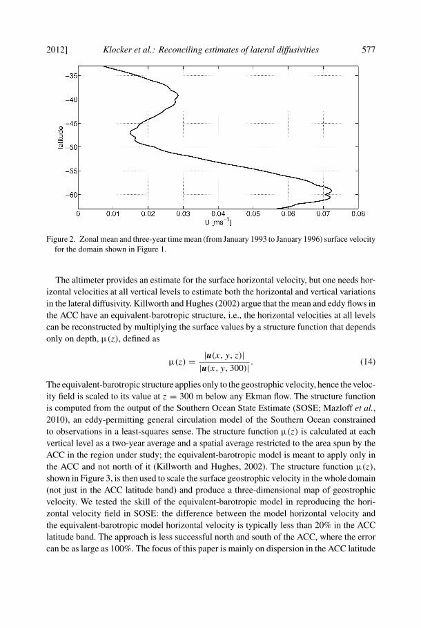
The altimeter provides an estimate for the surface horizontal velocity, but one needs hor-izontal velocities at all vertical levels to estimate both the horizontal and vertical variationsin the lateral diffusivity. Killworth and Hughes (2002) argue that the mean and eddy flows inthe ACC have an equivalent-barotropic structure, i.e., the horizontal velocities at all levelscan be reconstructed by multiplying the surface values by a structure function that dependsonly on depth, μ(z), defined as
μ(z) = |u(x, y, z)||u(x, y, 300)| . (14)
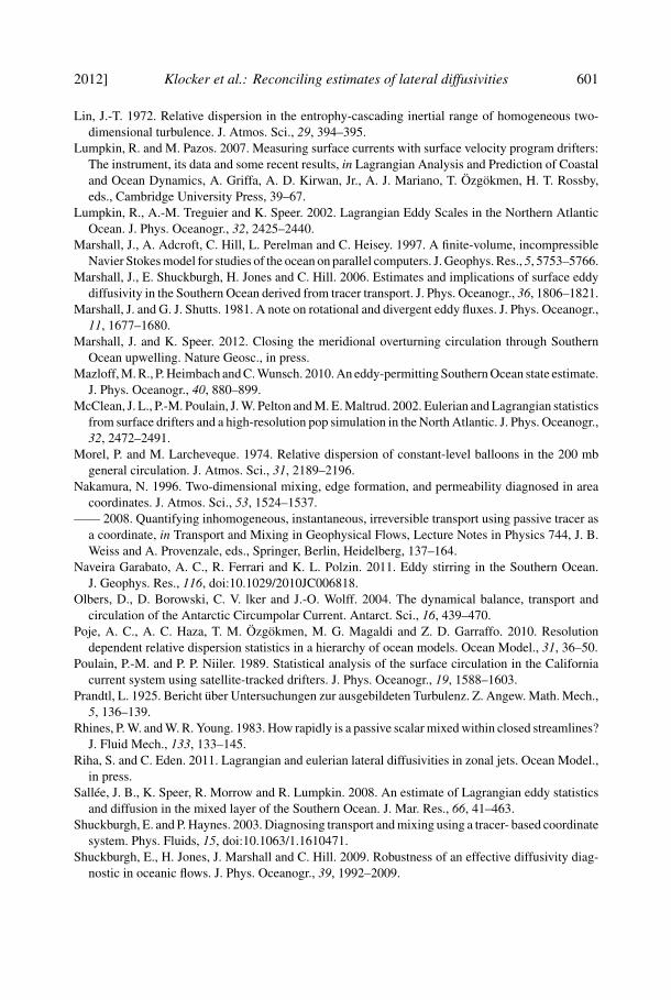
The equivalent-barotropic structure applies only to the geostrophic velocity, hence the veloc-ity field is scaled to its value at z = 300 m below any Ekman flow. The structure functionis computed from the output of the Southern Ocean State Estimate (SOSE; Mazloff et al.,2010), an eddy-permitting general circulation model of the Southern Ocean constrainedto observations in a least-squares sense. The structure function μ(z) is calculated at eachvertical level as a two-year average and a spatial average restricted to the area spun by theACC in the region under study; the equivalent-barotropic model is meant to apply only inthe ACC and not north of it (Killworth and Hughes, 2002). The structure function μ(z),shown in Figure 3, is then used to scale the surface geostrophic velocity in the whole domain(not just in the ACC latitude band) and produce a three-dimensional map of geostrophicvelocity. We tested the skill of the equivalent-barotropic model in reproducing the hori-zontal velocity field in SOSE: the difference between the model horizontal velocity andthe equivalent-barotropic model horizontal velocity is typically less than 20% in the ACClatitude band. The approach is less successful north and south of the ACC, where the errorcan be as large as 100%. The focus of this paper is mainly on dispersion in the ACC latitude
578 Journal of Marine Research [70, 4
Figure 3. The equivalent-barotopic structure function μ(z) = 〈|u(x, y, z)|/|u(x, y, 300)|〉 as a func-tion of depth calculated from SOSE and averaged over the ACC latitude band. Note that thevelocities are scaled relative to 300 m to avoid Ekman fluxes in the mixed layer.
band, so the lack of skill in reconstructing the velocity in other regions is less important.Moreover, our goal is to compare different diffusivity estimates using the same velocityfield, and it is not too important if some aspects of the field are not realistic.
This equivalent-barotropic map of geostrophic velocities has advantages over using thefull three-dimensional velocity field from numerical models such as SOSE: first, it providesa simple kinematic framework to test our theory—for example, we can easily modify themean flow without affecting the phase speed of the eddies; and second, we can easilyincrease the resolution of the numerical code used to advect floats and tracers, so as tominimize spurious numerical diffusion. Even though this velocity field is highly idealized,it captures the key kinematic properties of the full velocity field and generates diffusivitiesvery similar to those estimated by Abernathey et al. (2010), who computed diffusivitiesadvecting tracers with the SOSE three-dimensional velocity field.
All diffusivity estimates converge in less than a year, as shown below. We focus on disper-sion in the meridional direction, as noted; fluid parcels experience meridional displacementsof 100–200 km during the first year.
The advection of tracers and floats is purely horizontal, i.e., vertical velocities areignored. The vertical displacements experienced in a year are less than 10–100 m. Thusthe lateral dispersion is hardly affected by the additional vertical displacement. The
2012] Klocker et al.: Reconciling estimates of lateral diffusivities 579
vertical velocities are nevertheless important because they permit horizontal divergence(∂xu + ∂yv = −∂zw = 0 because of the latitudinal variation of the Coriolis parameter, thepresence of boundaries, and so on). Over long times, fluid particles would artificially clusterin regions of convergence and drift away from regions of divergence. We therefore make thevelocity field nondivergent by adding a divergent correction, Δχ, to the altimetric veloc-ity; i.e., we create a velocity field u = ug + Δχ, where ug is the geostrophic velocity. Thedivergent correction further imposes no-normal flow conditions at the continental and north-south boundaries of the computational domain. Periodic conditions are instead enforced atthe east-west boundaries. The implementation of the nondivergent correction is describedin detail in Marshall et al. (2006). In practice the adjustment leads to very small changes inthe geostrophic velocity field primarily at the boundaries. The estimates of dispersion arehardly sensitive to these corrections, except close to the meridional boundaries.
4. Methods
We now compare the effective diffusivity of Nakamura (1996) with the single-particleand two-particle diffusivities. We also estimate the diffusivity from the dispersion of tracerpatches. As the effective diffusivity measures mixing across the mean flow, which is pri-marily zonal in the region considered here, we focus solely on the meridional componentsof the diffusivities.
We compute the effective diffusivity Ke by advecting a tracer with the equivalent-barotropic velocity field shown in Figure 1 and using a constant numerical diffusivity κ. Theapproach is identical to that described in Marshall et al. (2006) and Ferrari and Nikurashin(2010) and the reader is referred to those papers for technical details. This requires carefulconsideration of the implicit mixing due to the numerical scheme that increases the value ofκ to be used in (4)—we show in the Appendix that the implicit mixing changes with depthand these variations must be taken into account.
The meridional component of the single-particle diffusivity is defined as
K1y(y0, t) = 1
2
d
dt〈(y(t) − y0)
2〉, (15)
where y(t) is the meridional position of a particle released at y0 at t = 0 and 〈·〉 is theaverage over all particles. We anticipate that the diffusivity will vary with latitude, so weexpress it as a function of the initial position, y0.
The eddy diffusivity is equal to the integral of the Lagrangian autocorrelation function:
K1y(y0, t) =∫ t
0Rvv(y0, τ) dτ where Rvv(y0, τ) = 〈vL(y0, τ)vL(y0, 0)〉, (16)
and vL(y0, t) is the Lagrangian velocity of a particle. Assuming that the correlation goes tozero after a given period of time and that its integral is finite, the diffusivity K1y(y0, t) willasymptote to a constant value (Taylor, 1921).
580 Journal of Marine Research [70, 4
The relative (two-particle) diffusivity is defined analogously:
K2y(y0, �r0, t) = 1
4
d
dt〈(yi(t) − yj (t))
2〉, (17)
where yi(t) and yj (t) are the meridional positions of particles i and j released within adistance �r0 of each other (y0 is the initial condition of either the i or j particle); theensemble average is taken over many such pairs. As noted, we use the pre-factor of one-fourth to ensure that the two-particle diffusivity asymptotes to the single-particle value atlong times (e.g., Davis, 1985).
Trajectories are generated by advecting numerical particles with the velocity fielddescribed above. The floats are initialized on a regular grid with an initial spacing of 0.2◦ andadvected for one year using a fourth-order Runge-Kutta scheme. Float positions are savedevery 0.6 days. We impose a periodic boundary condition in the zonal direction, so thatfloats leaving the eastern or western boundary reenter from the opposite side. This ensuresthat floats do not leave the computational domain, increasing the length of the particle timeseries. A no-normal flow condition is imposed at the northern and southern boundaries(Section 3), so the floats are unable to leave there.
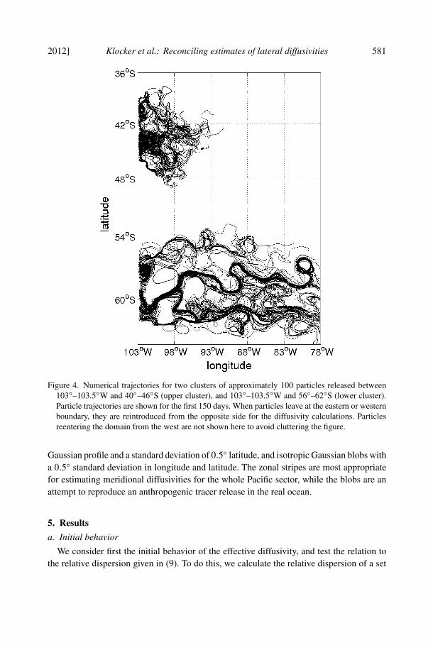
A few sample trajectories illustrate the different kinematic regimes in the subtropicalgyre and in the ACC (Fig. 4). In the subtropical gyre, the floats have a random motion.In the ACC, on the other hand, the particles exhibit coherent, meandering motion. Thismeandering plays an important role in the subsequent particle statistics. Note that after150 days many floats in the ACC would have left the domain from the east, were they notreintroduced from the west (reentering floats are not shown in the figure).
Lastly, there is the diffusivity derived from the dispersion of a cloud of tracer. The centeredsecond moment of the cloud is equivalent to the relative dispersion of all pairs of particlesin the cloud. When the pair motions become uncorrelated, the centered second moment ofthe cloud increases linearly in time, as for a diffusive process; at this point the diffusivitycan be obtained from the time derivative of the centered second moment (Garrett, 1983).The meridional component is defined
Kty = 1
2
∂σ2y
∂t= 1
2
∂
∂t
∫∫(y − yc)
2C(x, y)dxdy∫∫C(x, y)dxdy
, (18)
where σ2y is the second moment of the tracer concentration in latitude and yc is the meridional
position of the baricenter of the tracer patch,
yc =∫∫
yC(x, y)dxdy∫∫C(x, y)dxdy
. (19)
We advected tracer patches with the same velocity field and numerical scheme describedbefore. We used two different initial conditions: zonally uniform stripes with a meridional
2012] Klocker et al.: Reconciling estimates of lateral diffusivities 581
Figure 4. Numerical trajectories for two clusters of approximately 100 particles released between103◦–103.5◦W and 40◦–46◦S (upper cluster), and 103◦–103.5◦W and 56◦–62◦S (lower cluster).Particle trajectories are shown for the first 150 days. When particles leave at the eastern or westernboundary, they are reintroduced from the opposite side for the diffusivity calculations. Particlesreentering the domain from the west are not shown here to avoid cluttering the figure.
Gaussian profile and a standard deviation of 0.5◦ latitude, and isotropic Gaussian blobs witha 0.5◦ standard deviation in longitude and latitude. The zonal stripes are most appropriatefor estimating meridional diffusivities for the whole Pacific sector, while the blobs are anattempt to reproduce an anthropogenic tracer release in the real ocean.
5. Results
a. Initial behavior
We consider first the initial behavior of the effective diffusivity, and test the relation tothe relative dispersion given in (9). To do this, we calculate the relative dispersion of a set
582 Journal of Marine Research [70, 4
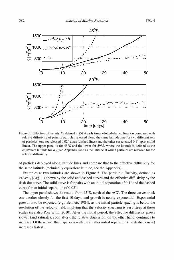
Figure 5. Effective diffusivity Ke defined in (5) at early times (dotted-dashed lines) as compared withrelative diffusivity of pairs of particles released along the same latitude line for two different setsof particles, one set released 0.02◦ apart (dashed lines) and the other set released 0.1◦ apart (solidlines). The upper panel is for 45◦S and the lower for 59◦S, where the latitude is defined as theequivalent latitude for Ke (see Appendix) and as the latitude at which particles are released for therelative diffusivity.
of particles deployed along latitude lines and compare that to the effective diffusivity forthe same latitude (technically equivalent latitude, see the Appendix).
Examples at two latitudes are shown in Figure 5. The particle diffusivity, defined asκ〈�r2〉/〈�r2
0 〉, is shown by the solid and dashed curves and the effective diffusivity by thedash-dot curve. The solid curve is for pairs with an initial separation of 0.1◦ and the dashedcurve for an initial separation of 0.02◦.
The upper panel shows the results from 45◦S, north of the ACC. The three curves trackone another closely for the first 10 days, and growth is nearly exponential. Exponentialgrowth is to be expected (e.g., Bennett, 1984), as the initial particle spacing is below theresolution of the velocity field, implying that the velocity spectrum is very steep at thesescales (see also Poje et al., 2010). After the initial period, the effective diffusivity growsslower (and saturates, soon after); the relative dispersion, on the other hand, continues toincrease. Of these two, the dispersion with the smaller initial separation (the dashed curve)increases fastest.
2012] Klocker et al.: Reconciling estimates of lateral diffusivities 583
The latter effect can be understood as follows. All the curves have the same initial value,equal to κ. Imagine that the exponential growth proceeds to a scale, L; this could be thedeformation radius, for example. At that scale, the particle estimate of the dispersion from(6) is κL2/ � r2
0 . So the smaller the initial spacing, the larger the diffusivity at scale L.In addition, the exponential growth is clearest with the �r0 = 0.02◦ spacing, as the pairsexperience the interpolated velocity differences for a longer period.
The comparison at 59◦S, in the ACC latitude band, is not as good. The particle dispersionincreases exponentially and the two curves with different initial separations agree with oneanother at early times, as before. But both grow more rapidly than the effective diffusivity.The latter asymptotes to a value near 500 m2s−1 by day 25, while the particle-based estimatesare much larger.
This suggests that the mean flow causes the effective diffusivity to diverge faster fromthe area-conserving estimate given in (6). This is due in part to the zonal dispersion ofthe particles by the mean flow. Rhines and Young (1983) show that tracers are rapidlyhomogenized along mean streamlines, so after a very short transient the tracer contoursreflect only the cross-flow diffusivity. But the two-particle dispersion used to evaluate L2
also includes the zonal dispersion, and this is increasing faster due to the mean shear.In summary, the effective diffusivity behaves like the relative dispersion of particle pairs
initially. But at later times, when the effective diffusivity asymptotes, the similarity nolonger holds. This is due in part to the nonconservation of area between tracer contours andbecause the effective diffusivity measures only the cross-flow diffusivity. Thus having amean zonal flow worsens the agreement and it is more sensible to focus on the cross-streamparticle diffusivity at later times.
b. Asymptotic behavior; effective diffusivity
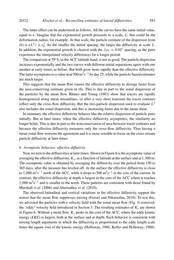
Now we turn to the diffusivities at later times. Shown in Figure 6 is the asymptotic value ofaveraging the effective diffusivity, Ke, as a function of latitude at the surface and at 1,500 m.The asymptotic value is obtained by averaging the diffusivity over the period from 150 to365 days, after the measure has leveled off. At the surface the effective diffusivity is closeto 1,000 m2s−1 north of the ACC, while it drops to 500 m2s−1 in the core of the current. Incontrast, the effective diffusivity at depth is largest in the core of the ACC where it reaches1,000 m2s−1 and is smaller to the north. These patterns are consistent with those found byMarshall et al. (2006) and Abernathey et al. (2010).
The observed latitudinal and vertical variations in the effective diffusivity support thenotion that the mean flow suppresses mixing (Ferrari and Nikurashin, 2010). To test this,we advected the particles with a velocity field with the zonal mean flow (Fig. 3) removed:the “eddy” velocity field introduced in Section 3. The resulting estimates of Ke are shownin Figure 6. Without a mean flow, Ke peaks in the core of the ACC, where the eddy kineticenergy (EKE) is largest, both at the surface and at depth. Such behavior is consistent withmixing length arguments in which the diffusivity is proportional to the eddy length scaletimes the square root of the kinetic energy (Holloway, 1986; Keffer and Holloway, 1988).
584 Journal of Marine Research [70, 4
Figure 6. Effective diffusivity Ke (solid blue lines), defined in (5), and tracer-based diffusivity Kty ,defined in (18), from the spreading of tracer stripes (solid black lines) and tracer patches (solidred lines). Also shown is the effective diffusivity for a tracer advected with the eddy velocityonly (dashed blue lines). (a) Diffusivities computed with the surface geostrophic velocity field. (b)Diffusivities calculated with the equivalent-barotropic velocity field rescaled for ∼1,500 m.
The eddy length scale varies little with depth and latitude, so that Ke ∝ √EKE. However,
the addition of a mean flow breaks the scaling at the surface (at depth the mean flow is veryweak). The suppression is more pronounced in the ACC where the mean flow is largest.The suppression of mixing by the mean flow is the focus of a companion paper (Klockeret al., 2012).
2012] Klocker et al.: Reconciling estimates of lateral diffusivities 585
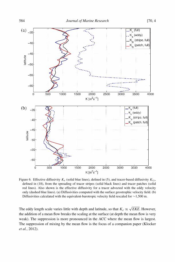
Figure 7. Latitude-depth maps of (a) effective diffusivity Ke (5) and (b) the single-particle diffusivityK1y (15) [m2s−1]. Diffusivities were calculated at 10 depth levels, using the equivalent-barotropicvelocity field described in Section 3.
Figure 7a shows the full latitude-depth map of Ke for the Pacific sector under study. Inthe ACC latitude band, between 55◦ and 65◦S, the effective diffusivity is suppressed by themean flow at the surface and has a subsurface maximum around 1,500 m where the meanflow becomes weak. To the north, where the mean flows are weaker, the effective diffusivityis largest at the surface where the EKE is largest.
c. Moment method: dispersion of a tracer stripes and patches
Next we consider the diffusivities as estimated from the growth of a patch of tracer.Figure 6 shows the diffusivity for a series of zonal “stripes” of tracer, released at different
586 Journal of Marine Research [70, 4
latitudes at the surface and at 1,500 m. The growth rate of σ2y becomes linear in time after
150 days. We estimate the diffusivity Kty as a least square fit of the change in σ2y versus
time between 150 and 365 days. The Kty values estimated from (18) agree well with theeffective diffusivities Ke at all latitudes, despite some discrepancies at the northern andsouthern boundaries, where edge effects suppress the dispersion.
Results from the Gaussian patch releases are also shown in Figure 6. Tracer patches werereleased at 100◦W at a set of different latitudes spaced by one degree, at the surface andat 1,500 m. The initial transient is much more variable in these simulations, but after 150days the dispersion is increasing linearly and diffusivities are computed in the same wayas done for the tracer stripes. Agreement with the previous estimates is very good. Againdiscrepancies are visible at the north and south edges of the domain, and also between 53◦and 54◦S. The latter is the result of the rapid zonal variations in eddy diffusivity at thenorthern edge of the ACC.
Note that while the effective diffusivity and the zonal stripes yield a zonal average of thediffusivity, the Gaussian patches at early times can be used to detect longitudinal variations.Averaging the results from patches released across the domain in the zonal direction yieldsthe same diffusivity as with the stripe (not shown here). Note that agreement betweendifferent methods is achieved because we can sample all of the tracer (periodic boundaryconditions ensure that the tracer never leaves the domain). Such sampling cannot be donein field experiments.
d. Particle dispersion
Lastly, we consider diffusivities derived from particle trajectories. We begin with single-particle diffusivity, as this is the measure used most frequently in observational studies. Wecalculated K1y(y0, t) using (15)—estimating the diffusivity by integrating the velocity auto-correlation yielded identical results. We averaged the diffusivities for all particles deployedin regions 25◦ in longitude (the width of the domain) by 2◦ in latitude. This averaging stripeis substantially larger than the typical eddy scale in the Southern Ocean of O(100) km. Asthe mean velocity is purely zonal, we do not need to separate mean and eddy velocities inthe meridional direction.
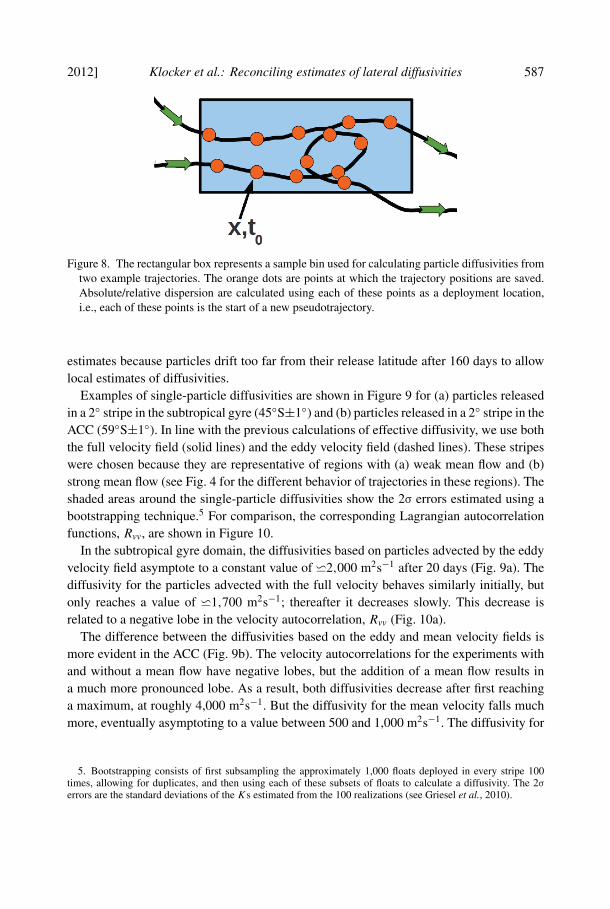
Following Davis (1991), we treat every point at which a float position is saved as a startingposition for a new trajectory, substantially increasing the number of pseudotrajectories. Themethod is illustrated graphically in Figure 8: every orange dot shows a point at which afloat position is saved, and it is treated as the starting position for a new trajectory. Thetechnique is described by Griesel et al. (2010) and represents a slight modification of thetechnique used in Colin de Verdiere (1983), Poulain and Niiler (1989) and Zhurbas and Oh(2003), among others. The single-particle diffusivities converge to a constant within half ayear in the subtropical gyres and sooner elsewhere. Hence we consider all trajectories with aminimum length of 160 days and estimate the diffusivity as an average over the last 20 daysof all available pseudotrajectories. The averaging window is different from tracer-based
2012] Klocker et al.: Reconciling estimates of lateral diffusivities 587
Figure 8. The rectangular box represents a sample bin used for calculating particle diffusivities fromtwo example trajectories. The orange dots are points at which the trajectory positions are saved.Absolute/relative dispersion are calculated using each of these points as a deployment location,i.e., each of these points is the start of a new pseudotrajectory.
estimates because particles drift too far from their release latitude after 160 days to allowlocal estimates of diffusivities.
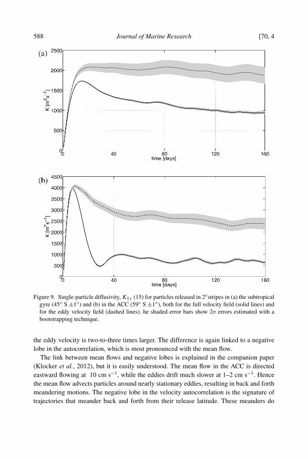
Examples of single-particle diffusivities are shown in Figure 9 for (a) particles releasedin a 2◦ stripe in the subtropical gyre (45◦S±1◦) and (b) particles released in a 2◦ stripe in theACC (59◦S±1◦). In line with the previous calculations of effective diffusivity, we use boththe full velocity field (solid lines) and the eddy velocity field (dashed lines). These stripeswere chosen because they are representative of regions with (a) weak mean flow and (b)strong mean flow (see Fig. 4 for the different behavior of trajectories in these regions). Theshaded areas around the single-particle diffusivities show the 2σ errors estimated using abootstrapping technique.5 For comparison, the corresponding Lagrangian autocorrelationfunctions, Rvv, are shown in Figure 10.
In the subtropical gyre domain, the diffusivities based on particles advected by the eddyvelocity field asymptote to a constant value of �2,000 m2s−1 after 20 days (Fig. 9a). Thediffusivity for the particles advected with the full velocity behaves similarly initially, butonly reaches a value of �1,700 m2s−1; thereafter it decreases slowly. This decrease isrelated to a negative lobe in the velocity autocorrelation, Rvv (Fig. 10a).
The difference between the diffusivities based on the eddy and mean velocity fields ismore evident in the ACC (Fig. 9b). The velocity autocorrelations for the experiments withand without a mean flow have negative lobes, but the addition of a mean flow results ina much more pronounced lobe. As a result, both diffusivities decrease after first reachinga maximum, at roughly 4,000 m2s−1. But the diffusivity for the mean velocity falls muchmore, eventually asymptoting to a value between 500 and 1,000 m2s−1. The diffusivity for
5. Bootstrapping consists of first subsampling the approximately 1,000 floats deployed in every stripe 100times, allowing for duplicates, and then using each of these subsets of floats to calculate a diffusivity. The 2σ
errors are the standard deviations of the Ks estimated from the 100 realizations (see Griesel et al., 2010).
588 Journal of Marine Research [70, 4
Figure 9. Single-particle diffusivity, K1y (15) for particles released in 2◦stripes in (a) the subtropicalgyre (45◦ S ±1◦) and (b) in the ACC (59◦ S ±1◦), both for the full velocity field (solid lines) andfor the eddy velocity field (dashed lines). he shaded error bars show 2σ errors estimated with abootstrapping technique.
the eddy velocity is two-to-three times larger. The difference is again linked to a negativelobe in the autocorrelation, which is most pronounced with the mean flow.
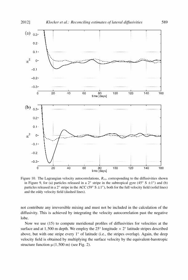
The link between mean flows and negative lobes is explained in the companion paper(Klocker et al., 2012), but it is easily understood. The mean flow in the ACC is directedeastward flowing at 10 cm s−1, while the eddies drift much slower at 1–2 cm s−1. Hencethe mean flow advects particles around nearly stationary eddies, resulting in back and forthmeandering motions. The negative lobe in the velocity autocorrelation is the signature oftrajectories that meander back and forth from their release latitude. These meanders do
2012] Klocker et al.: Reconciling estimates of lateral diffusivities 589
Figure 10. The Lagrangian velocity autocorrelations, Rvv, corresponding to the diffusivities shownin Figure 9, for (a) particles released in a 2◦ stripe in the subtropical gyre (45◦ S ±1◦) and (b)particles released in a 2◦ stripe in the ACC (59◦ S ±1◦), both for the full velocity field (solid lines)and the eddy velocity field (dashed lines).
not contribute any irreversible mixing and must not be included in the calculation of thediffusivity. This is achieved by integrating the velocity autocorrelation past the negativelobe.
Now we use (15) to compute meridional profiles of diffusivities for velocities at thesurface and at 1,500 m depth. We employ the 25◦ longitude × 2◦ latitude stripes describedabove, but with one stripe every 1◦ of latitude (i.e., the stripes overlap). Again, the deepvelocity field is obtained by multiplying the surface velocity by the equivalent-barotropicstructure function μ(1,500 m) (see Fig. 2).
590 Journal of Marine Research [70, 4
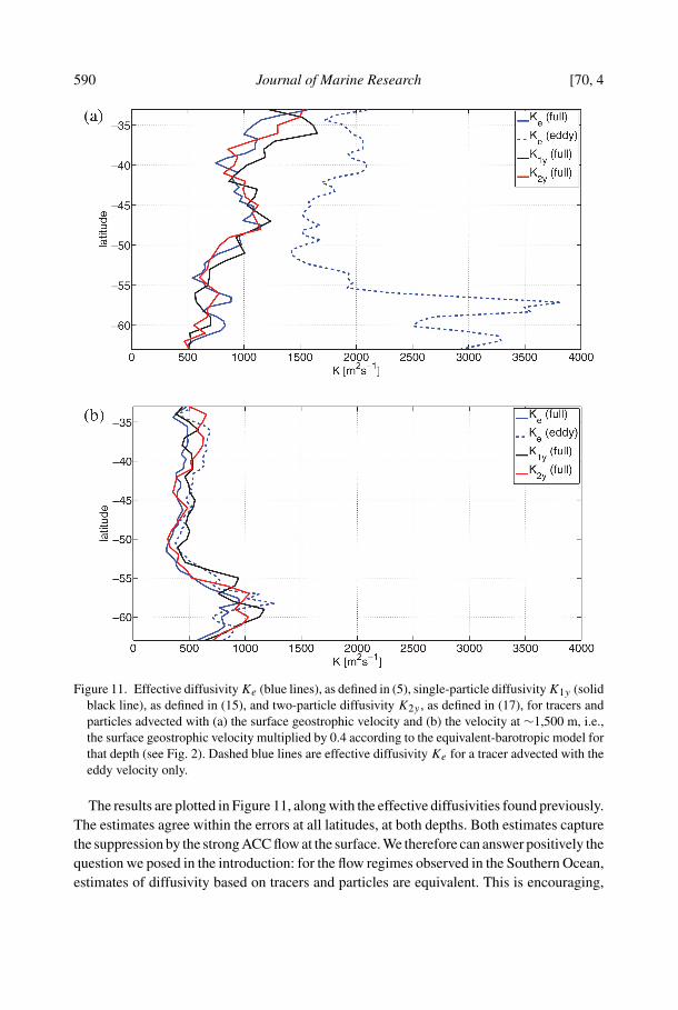
Figure 11. Effective diffusivity Ke (blue lines), as defined in (5), single-particle diffusivity K1y (solidblack line), as defined in (15), and two-particle diffusivity K2y , as defined in (17), for tracers andparticles advected with (a) the surface geostrophic velocity and (b) the velocity at ∼1,500 m, i.e.,the surface geostrophic velocity multiplied by 0.4 according to the equivalent-barotropic model forthat depth (see Fig. 2). Dashed blue lines are effective diffusivity Ke for a tracer advected with theeddy velocity only.
The results are plotted in Figure 11, along with the effective diffusivities found previously.The estimates agree within the errors at all latitudes, at both depths. Both estimates capturethe suppression by the strong ACC flow at the surface. We therefore can answer positively thequestion we posed in the introduction: for the flow regimes observed in the Southern Ocean,estimates of diffusivity based on tracers and particles are equivalent. This is encouraging,
2012] Klocker et al.: Reconciling estimates of lateral diffusivities 591
because numerical models need the diffusivity that describes the rate at which tracers arehomogenized, while direct estimates of diffusivity in the ocean rely on float dispersion(especially below the surface). Agreement between the two estimates means that we cancompare models and observations.
In a number of previous studies, the single-particle diffusivity was estimated either fromthe maximum value achieved by K1y at short times (e.g., Zhurbas and Oh, 2003) or, equiva-lently, by integrating to the first zero crossing of the velocity autocorrelation (e.g., Freelandet al., 1975; Poulain and Niiler, 1989). The reasoning is that the error in the diffusivitygrows in time, so that the estimates at longer lags are less certain. However, ignoring thecontribution of the negative lobe results in a substantial overestimate of K1y . An option israther to fit the autocorrelation to the product of an exponential and a cosine (Garraffo et al.,2001; Sallée et al., 2008). This is in line with the present findings.
Integrating our velocity autocorrelations to the first zero crossing or equivalently using themaximum yields much larger diffusivities (not shown). Moreover, there was little differencebetween the diffusivities found using the full velocity and the eddy velocity. Thus usingthe first zero crossing method effectively misses the suppression of eddy diffusivity by themean flow.
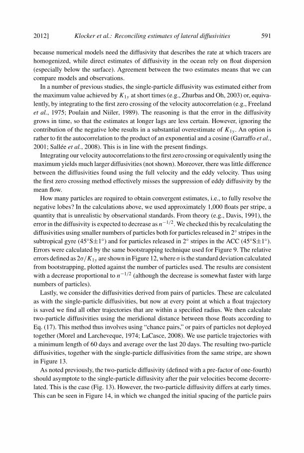
How many particles are required to obtain convergent estimates, i.e., to fully resolve thenegative lobes? In the calculations above, we used approximately 1,000 floats per stripe, aquantity that is unrealistic by observational standards. From theory (e.g., Davis, 1991), theerror in the diffusivity is expected to decrease as n−1/2. We checked this by recalculating thediffusivities using smaller numbers of particles both for particles released in 2◦ stripes in thesubtropical gyre (45◦S±1◦) and for particles released in 2◦ stripes in the ACC (45◦S±1◦).Errors were calculated by the same bootstrapping technique used for Figure 9. The relativeerrors defined as 2σ/K1y are shown in Figure 12, where σ is the standard deviation calculatedfrom bootstrapping, plotted against the number of particles used. The results are consistentwith a decrease proportional to n−1/2 (although the decrease is somewhat faster with largenumbers of particles).
Lastly, we consider the diffusivities derived from pairs of particles. These are calculatedas with the single-particle diffusivities, but now at every point at which a float trajectoryis saved we find all other trajectories that are within a specified radius. We then calculatetwo-particle diffusivities using the meridional distance between those floats according toEq. (17). This method thus involves using “chance pairs,” or pairs of particles not deployedtogether (Morel and Larcheveque, 1974; LaCasce, 2008). We use particle trajectories witha minimum length of 60 days and average over the last 20 days. The resulting two-particlediffusivities, together with the single-particle diffusivities from the same stripe, are shownin Figure 13.
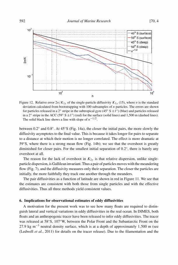
As noted previously, the two-particle diffusivity (defined with a pre-factor of one-fourth)should asymptote to the single-particle diffusivity after the pair velocities become decorre-lated. This is the case (Fig. 13). However, the two-particle diffusivity differs at early times.This can be seen in Figure 14, in which we changed the initial spacing of the particle pairs
592 Journal of Marine Research [70, 4
Figure 12. Relative error 2σ/K1y of the single-particle diffusivity K1y (15), where σ is the standarddeviation calculated from bootstrapping with 100 subsamples of n particles. The errors are shownfor particles released in a 2◦ stripe in the subtropical gyre (45◦ S ±1◦) (blue) and particles releasedin a 2◦ stripe in the ACC (59◦ S ±1◦) (red) for the surface (solid lines) and 1,500 m (dashed lines).The solid black line shows a line with slope of n−1/2.
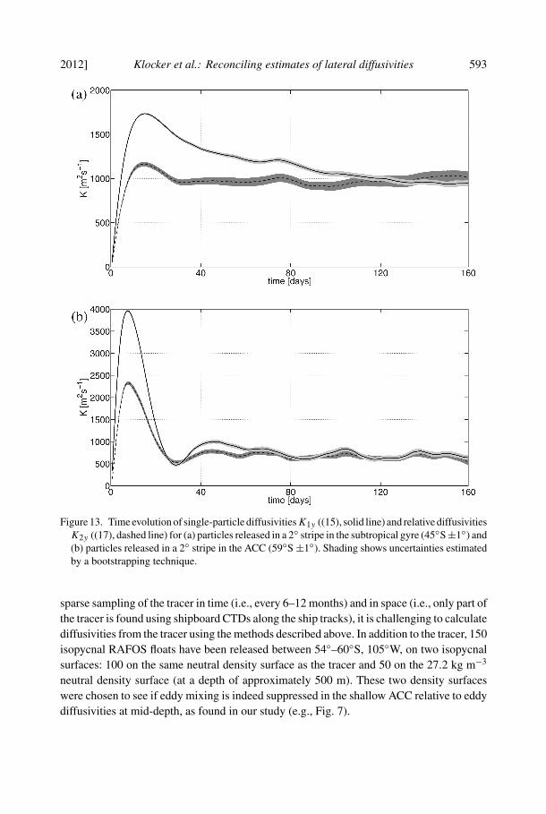
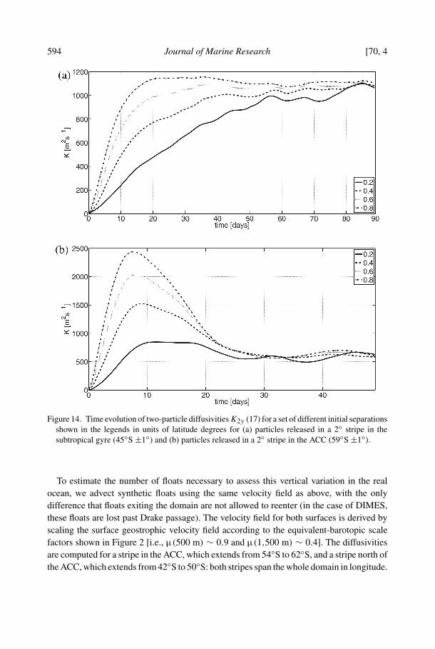
between 0.2◦ and 0.8◦. At 45◦S (Fig. 14a), the closer the initial pairs, the more slowly thediffusivity asymptotes to the final value. This is because it takes longer for pairs to separateto a distance at which their motion is no longer correlated. The effect is more dramatic at59◦S, where there is a strong mean flow (Fig. 14b); we see that the overshoot is greatlydiminished for closer pairs. For the smallest initial separation of 0.2◦, there is barely anyovershoot at all.
The reason for the lack of overshoot in K2y is that relative dispersion, unlike single-particle dispersion, is Gallilean invariant. Thus a pair of particles moves with the meanderingflow (Fig. 7), and the diffusivity measures only their separation. The closer the particles areinitially, the more faithfully they track one another through the meanders.
The pair diffusivities as a function of latitude are shown in red in Figure 11. We see thatthe estimates are consistent with both those from single particles and with the effectivediffusivities. Thus all three methods yield consistent values.
6. Implications for observational estimates of eddy diffusivities
A motivation for the present work was to see how many floats are required to distin-guish lateral and vertical variations in eddy diffusivities in the real ocean. In DIMES, bothfloats and an anthropogenic tracer have been released to infer eddy diffusivities. The tracerwas released at 58◦S, 107◦W, between the Polar Front and the Subantarctic Front on the27.9 kg m−3 neutral density surface, which is at a depth of approximately 1,500 m (see(Ledwell et al., 2011) for details on the tracer release). Due to the filamentation and the
2012] Klocker et al.: Reconciling estimates of lateral diffusivities 593
Figure 13. Time evolution of single-particle diffusivitiesK1y ((15), solid line) and relative diffusivitiesK2y ((17), dashed line) for (a) particles released in a 2◦ stripe in the subtropical gyre (45◦S ±1◦) and(b) particles released in a 2◦ stripe in the ACC (59◦S ±1◦). Shading shows uncertainties estimatedby a bootstrapping technique.
sparse sampling of the tracer in time (i.e., every 6–12 months) and in space (i.e., only part ofthe tracer is found using shipboard CTDs along the ship tracks), it is challenging to calculatediffusivities from the tracer using the methods described above. In addition to the tracer, 150isopycnal RAFOS floats have been released between 54◦–60◦S, 105◦W, on two isopycnalsurfaces: 100 on the same neutral density surface as the tracer and 50 on the 27.2 kg m−3
neutral density surface (at a depth of approximately 500 m). These two density surfaceswere chosen to see if eddy mixing is indeed suppressed in the shallow ACC relative to eddydiffusivities at mid-depth, as found in our study (e.g., Fig. 7).
594 Journal of Marine Research [70, 4
Figure 14. Time evolution of two-particle diffusivities K2y (17) for a set of different initial separationsshown in the legends in units of latitude degrees for (a) particles released in a 2◦ stripe in thesubtropical gyre (45◦S ±1◦) and (b) particles released in a 2◦ stripe in the ACC (59◦S ±1◦).
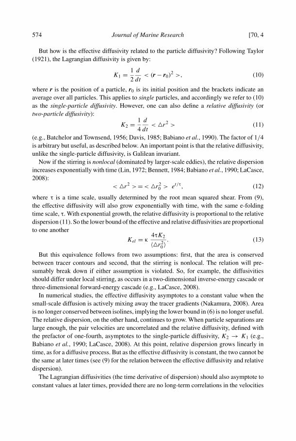
To estimate the number of floats necessary to assess this vertical variation in the realocean, we advect synthetic floats using the same velocity field as above, with the onlydifference that floats exiting the domain are not allowed to reenter (in the case of DIMES,these floats are lost past Drake passage). The velocity field for both surfaces is derived byscaling the surface geostrophic velocity field according to the equivalent-barotopic scalefactors shown in Figure 2 [i.e., μ(500 m) ∼ 0.9 and μ(1,500 m) ∼ 0.4]. The diffusivitiesare computed for a stripe in the ACC, which extends from 54◦S to 62◦S, and a stripe north ofthe ACC, which extends from 42◦S to 50◦S: both stripes span the whole domain in longitude.
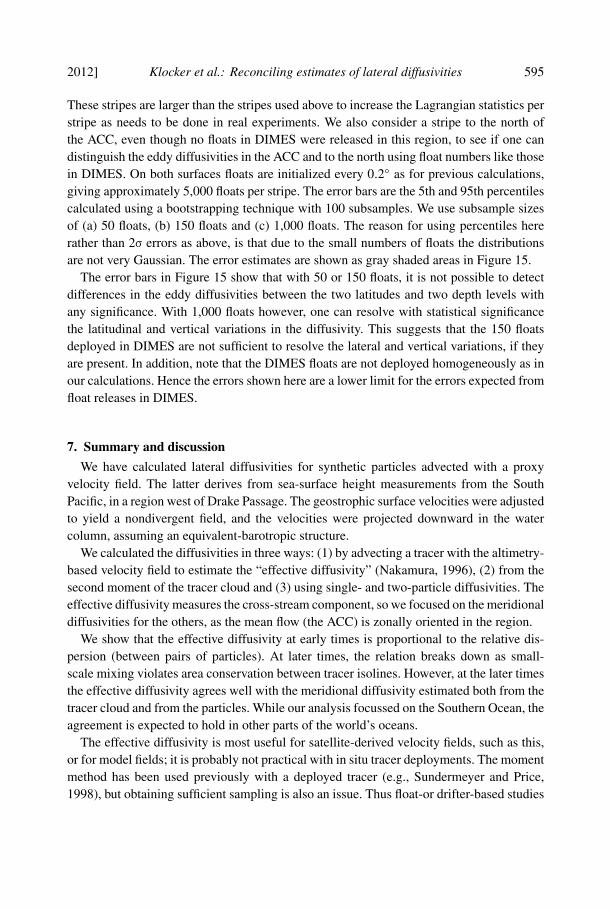
2012] Klocker et al.: Reconciling estimates of lateral diffusivities 595
These stripes are larger than the stripes used above to increase the Lagrangian statistics perstripe as needs to be done in real experiments. We also consider a stripe to the north ofthe ACC, even though no floats in DIMES were released in this region, to see if one candistinguish the eddy diffusivities in the ACC and to the north using float numbers like thosein DIMES. On both surfaces floats are initialized every 0.2◦ as for previous calculations,giving approximately 5,000 floats per stripe. The error bars are the 5th and 95th percentilescalculated using a bootstrapping technique with 100 subsamples. We use subsample sizesof (a) 50 floats, (b) 150 floats and (c) 1,000 floats. The reason for using percentiles hererather than 2σ errors as above, is that due to the small numbers of floats the distributionsare not very Gaussian. The error estimates are shown as gray shaded areas in Figure 15.
The error bars in Figure 15 show that with 50 or 150 floats, it is not possible to detectdifferences in the eddy diffusivities between the two latitudes and two depth levels withany significance. With 1,000 floats however, one can resolve with statistical significancethe latitudinal and vertical variations in the diffusivity. This suggests that the 150 floatsdeployed in DIMES are not sufficient to resolve the lateral and vertical variations, if theyare present. In addition, note that the DIMES floats are not deployed homogeneously as inour calculations. Hence the errors shown here are a lower limit for the errors expected fromfloat releases in DIMES.
7. Summary and discussion
We have calculated lateral diffusivities for synthetic particles advected with a proxyvelocity field. The latter derives from sea-surface height measurements from the SouthPacific, in a region west of Drake Passage. The geostrophic surface velocities were adjustedto yield a nondivergent field, and the velocities were projected downward in the watercolumn, assuming an equivalent-barotropic structure.
We calculated the diffusivities in three ways: (1) by advecting a tracer with the altimetry-based velocity field to estimate the “effective diffusivity” (Nakamura, 1996), (2) from thesecond moment of the tracer cloud and (3) using single- and two-particle diffusivities. Theeffective diffusivity measures the cross-stream component, so we focused on the meridionaldiffusivities for the others, as the mean flow (the ACC) is zonally oriented in the region.
We show that the effective diffusivity at early times is proportional to the relative dis-persion (between pairs of particles). At later times, the relation breaks down as small-scale mixing violates area conservation between tracer isolines. However, at the later timesthe effective diffusivity agrees well with the meridional diffusivity estimated both from thetracer cloud and from the particles. While our analysis focussed on the Southern Ocean, theagreement is expected to hold in other parts of the world’s oceans.
The effective diffusivity is most useful for satellite-derived velocity fields, such as this,or for model fields; it is probably not practical with in situ tracer deployments. The momentmethod has been used previously with a deployed tracer (e.g., Sundermeyer and Price,1998), but obtaining sufficient sampling is also an issue. Thus float-or drifter-based studies
Figu
re15
.Si
ngle
-par
ticle
diff
usiv
ityK
1y(1
5)fo
rpa
rtic
les
rele
ased
ina
stri
peno
rth
ofth
eA
CC
(a)
at50
0m
and
(b)
at15
00m
(the
stri
peex
tend
sfr
om44
◦ to
48◦ S
),an
dfo
rpa
rtic
les
rele
ased
ina
stri
pein
the
AC
C(c
)at
500
man
d(d
)at
1500
m(t
hest
ripe
exte
nds
from
56◦ t
o60
◦ S).
Gra
ysh
adin
gsh
ows
the
5th
and
95th
perc
entil
esde
term
ined
with
abo
otst
rapp
ing
tech
niqu
ew
ith10
0su
bsam
ples
,usi
ng50
float
s(d
ark
gray
),15
0flo
ats
(med
ium
gray
)an
d1,
000
float
s(l
ight
gray
).
2012] Klocker et al.: Reconciling estimates of lateral diffusivities 597
are still the most desirable. The present results demonstrate that the float-derived estimatesare consistent with the others, as long as they are calculated correctly.
Abernathey (2012) further shows that the effective diffusivity is equivalent to the eddydiffusivity based on a flux-gradient relationship across the mean current as per (1). His resultsare also obtained by numerically advecting tracers with satellite-derived velocity fields inregions where the mean ocean flows are primarily zonal. This result nicely complementsours, and we can conclude that all estimates of diffusivities based on floats and tracersconverge for the Southern Ocean flow regime considered in this paper.
A critical issue, seen clearly here, is that a mean flow suppresses the cross-stream dif-fusivities (e.g., Ferrari and Nikurashin, 2010; Naveira Garabato et al., 2011). One findsthat the particle-based diffusivity reaches a maximum value before decreasing to a lowerasymptotic limit. This reduction, often seen in observations, reflects a negative lobe in thevelocity autocorrelation. Physically, this corresponds to “meandering” motion—particlesbeing advected first across the mean flow and then returning some distance back towardtheir starting location. Thus the initial maximum is a transient advective feature and does notreflect the true mixing. Indeed, a similar overshoot is not seen with the effective diffusivity.Given this, using the maximum diffusivity, or equivalently integrating the autocorrelationto the first zero crossing, yields artificially large diffusivities.
There are two ways around this. One is to average the diffusivity after the initial transientphase, i.e., after it has reached the lower asymptotic limit. This means choosing an “inter-mediate” averaging period, after the initial transient but before the measurement errors havegrown too large (e.g., Koszalka and LaCasce, 2010). The second is to use the two-particlediffusivity, which relates to the separation between pairs of particles. As both particles inthe pair experience the initial meander, the relative diffusivity is devoid of the initial maxi-mum provided the initial pair separation is small enough. However, this requires having asufficient number of pairs to obtain reliable statistics.
Our results for the Pacific sector suggest that the number of particles or particle pairsnecessary to resolve the vertical and horizontal variations in eddy diffusivities are in thehundreds. The CARTHE experiment (Consortium for Advanced Research on Transport andHydrocarbon in the Environment), (www.carthe.org) underway in the Gulf of Mexico, useshundreds of drifters, and the numbers are likely to increase as the cost of drifters decreasesfurther. However, these numbers are prohibitively large for most field experiments that relyon subsurface floats like DIMES. Thus float-derived estimates should be used in conjunctionwith other information to quantify the absolute values and the vertical and lateral structureof eddy diffusivities. This could come from the release of a tracer patch, such as in DIMES;satellite-derived geostrophic velocity fields; and high-resolution numerical models. Thechallenge is to learn how to combine such diverse data sets to obtain statistically robustestimates of diffusivities.
Alternatively there are intriguing new ideas on how to use the geometrical shape ofwhole trajectories to infer mixing rates (e.g., Thiffeault, 2010). Noboru Nakamura (pers.comm.) has also suggested that one may be able to estimate the effective diffusivity using a
598 Journal of Marine Research [70, 4
combination of floats and tracer measurements. Whether such approaches will alleviate theprohibitive demands on float numbers remains an open question and a worthwhile avenuefor future studies.
We note too that the present study was greatly simplified by having a purely zonal meanflow in the region of interest. Thus we were able to focus on the meridional component ofthe diffusivity, and because values were averaged along the whole channel, we did not haveto worry about skew fluxes/stokes drifts. Having a nonzonal mean flow further demandsisolating the cross-flow component. This can be achieved, for example, via a principalaxis decomposition on the symmetric portion of the diffusivity tensor, with the cross-flowdiffusive component represented by the minor principal component (Zhurbas and Oh, 2003,2004). But the present comments still apply in relation to that component—one must takeaccount of the negative lobe.
Acknowledgments. This work was done as part of the Diapycnal and Isopycnal Mixing Experimentin the Southern Ocean (DIMES). We wish to acknowledge the generous support of NSF throughawards OCE-0825376 (RF and AK) and OCE-0849233 (SM). We thank one anonymous reviewerand Noboru Nakamura for their constructive comments on the first draft. We also wish to thank allthe DIMES principal investigators for many useful discussions and suggestions.
APPENDIX
To advect a numerical tracer, we use the offline capabilities of the Massachusetts Instituteof Technology general circulation model (MITgcm; Marshall et al., 1997) with the nondi-vergent velocity field described above and solve the tracer advection-diffusion equation
∂
∂tC + u · ∇C = κ∇2C, (20)
where C is the tracer concentration and κ is the explicit numerical diffusivity. For the traceradvection we use an Adams-Bashforth time-stepping scheme and a centered second-orderadvection scheme to advect the tracer for one year. The domain is zonally periodic withno-flux boundary conditions imposed at the northern and southern boundaries. The initialtracer concentration increases linearly with latitude, with values of zero at the southernboundary and values of one at the northern boundaries. As shown by Shuckburgh et al.(2009), the calculations of effective diffusivities are not very sensitive to the tracer initialcondition.
The most problematic part in calculating effective diffusivities is the total numerical diffu-sivity. For an artificial tracer advected by a numerical model, this is the sum of the explicitand implicit numerical diffusivities. Without knowing the total numerical diffusivity butassuming that it is constant, one can determine the spatial structure of Ke, but to computemagnitudes of effective diffusivities one needs an estimate of the total numerical diffusivity(Shuckburgh et al., 2009). Marshall et al. (2006) show that the estimate of Ke becomes inde-pendent of numerical diffusivity only for large Péclet number, with Pe = ULeddy/κtotal ,
2012] Klocker et al.: Reconciling estimates of lateral diffusivities 599
where U is the characteristic scale of the velocity, Leddy is an eddy length scale and κtotal
is the total numerical diffusivity. This would suggest the use of a small κ for our calcula-tions. On the other hand, using a κ that is too small introduces implicit numerical diffusiongenerated by noise on the grid scale, which acts to increase κtotal . For every vertical levelwe choose an explicit numerical diffusivity small enough to ensure that the estimate of Ke
is independent of the numerical diffusivity, but large enough to keep the implicit numericaldiffusivity small. To estimate the total numerical diffusivity inherent in the advection of theartificial tracer we use the tracer variance equation,
1
2
∂〈C2〉∂t
= −κtotal〈|∇C|2〉, (21)
where 〈·〉 indicates the average over the domain. κtotal is the total numerical diffusivitynecessary to explain the decay of the observed tracer variance 〈C2〉.
Ke is estimated by advecting the tracer with an explicit numerical diffusivity of 10 m2s−1.Using (21) gives us the numerical background diffusivity inherent in the numerical advectioncode, κtotal , which varies from 30 m2s−1 at the surface to 11 m2s−1 at depth. Note that thisvariation of κtotal with depth can easily be accounted for in the two-dimensional calculationsperformed in this study, but might lead to serious issues in three-dimensional calculationsin which one value for κtotal is used at all depths.
We then use (5) to calculate Ke, where L0(yeq) is the width of the domain at the equivalentlatitude yeq , and L2
eq can be written as (see Shuckburgh and Haynes, 2003, for a derivation)
L2eq =
[1
( ∂C∂A
)
∂
∂A
∫A
|∇C|dA
]2
, (22)
where C is the tracer concentration and A is the area between tracer contours.
REFERENCES
Abernathey, R. 2012. Mixing by ocean eddies. Ph.D. thesis, Massachusetts Institute of Technology.Abernathey, R., J. Marshall, M. Mazloff and E. Shuckburgh. 2010. Critical layer enhancement of
mesoscale eddy stirring in the Southern Ocean. J. Phys. Oceanogr., 40, 170–184.Armi, L. and H. Stommel. 1983. Four views of a portion of the North Atlantic subtropical gyre.
J. Phys. Oceanogr., 13, 828–857.Babiano, A., C. Basdevant, P. LeRoy and R. Sadourny. 1990. Relative dispersion in two-dimensional
turbulence. J. Fluid Mech., 214, 535–557.Batchelor, G. K. and A. A. Townsend. 1956. Turbulent diffusion, in Surveys in Mechanics, G. K.
Batchelor and H. Bondi, eds., Cambridge University Press, Cambridge, 352–398.Bennett, A. F. 1984. Relative dispersion: Local and nonlocal dynamics. J. Atmos. Sci., 41, 1881–1886.—— 2006. Lagrangian Fluid Dynamics, Monographs on Mechanics, Cambridge University Press,
Cambridge. 286 pp.Bryden, H. L. and R. A. Heath. 1985. Energetic eddies at the northern edge of the Antarctic Circum-
polar Current. Progr. Oceanogr., 14, 65–87.
600 Journal of Marine Research [70, 4
Colin de Verdiere, A. 1983. Lagrangian eddy statistics from surface drifters in the eastern NorthAtlantic. J. Mar. Res., 41, 375–398.
Danabasoglu, G. and J. Marshall. 2007. Effects of vertical variations of thickness diffusivity in anocean general circulation model. Ocean Model., 18, 122–141.
Davis, R. 1985. Drifter observations of coastal surface currents during CODE: The statistical anddynamical view. J. Geophys. Res., 90, 4756–4772.
—— 1991. Observing the general circulation with floats. Deep-Sea Res., 38A, S531–S571.Ferrari, R. and M. Nikurashin. 2010. Suppression of eddy diffusivity across jets in the Southern Ocean.
J. Phys. Oceanogr., 40, 1501–1519.Ferrari, R. and K. L. Polzin. 2005. Finescale structure of the t-s relation in the eastern North Atlantic.
J. Phys. Oceanogr., 35, 1437–1454.Freeland, H., P. Rhines and T. Rossby. 1975. Statistical observations of the trajectories of neutrally
buoyant floats in the North Atlantic. J. Mar. Res., 33, 383–404.Garraffo, Z., A. Mariano, A. Griffa and C. Veneziani. 2001. Lagrangian data in a high-resolution
numerical simulation of the North Atlantic. I. Comparison with in-situ drifter data. J. Mar. Sys.,29, 157–176.
Garrett, C. 1983. On the initial streakiness of a dispersion tracer in two- and three-dimensionalturbulence. Dyn. Atmos. Oceans, 7, 265–277.
Griesel, A., S. T. Gille, J. Sprintall, L. McClean, J. H. LaCasce and M. E. Maltrud. 2010. Isopycnaldiffusivities in the Antarctic Circumpolar Current inferred from Lagrangian floats in an eddyingmodel. J. Mar. Res., 66, 441–463.
Griffies, S. M., A. Gnanadesikan, K. W. Dixon, J. P. Dunnee, R. Gerdes, M. J. Harrison, A. Rosati,J. L. Russell, B. L. Samuels, M. J. Spelman, M. Winton and R. Zhang. 2005. Formulation of anocean model for global climate simulations. Ocean Sci., 1, 45–79.
Holloway, G. 1986. Estimation of oceanic eddy transports from satellite altimetry. Nature, 323, 243–244.
Jenkins, W. J. 1998. Studying subtropical thermocline ventilation and circulation using tritium and3He. J. Geophys. Res., 103, 15187–15831.
Keffer, T. and G. Holloway. 1988. Estimating Southern Ocean eddy flux of heat and salt from satellitealtimetry. Nature, 332, 624–626.
Killworth, P. D. and C. W. Hughes. 2002. The Antarctic Circumpolar Current as a free equivalent-barotropic jet. J. Mar. Res., 60, 19–45.
Klocker, A., R. Ferrari and J. H. LaCasce. 2012. Estimating suppression of eddy mixing by meanflows. J. Phys. Oceanogr., 42, 1566–1576.
Koszalka, I. and J. H. LaCasce. 2010. Lagrangian analysis by clustering. Ocean Dyn., 60, 957–972.Krauss, W. and C. W. Böning. 1987. Lagrangian properties of eddy fields in the northern North
Atlantic as deduced from satellite-tracked buoys. J. Mar. Res., 45, 259–291.LaCasce, J. H. 2008. Statistics from Lagrangian observations. Progr. Oceanogr., 77, 1–29.Ledwell, J. R., L. C. St. Laurent, J. B. Girton and J. M. Toole. 2011. Diapycnal mixing in the Antarctic
Circumpolar Current. J. Phys. Oceanogr., 41, 241–246.Ledwell, J. R., A. J. Watson and C. S. Law. 1998. Mixing of a tracer in a pycnocline. J. Geophys.
Res., 103, 21499–21529.Lemoine, F. G., D. E. Smith, L. Kunz, R. Smith, N. K. Pavlis, S. M. Klosko, D. S. Chinn, M. H.
Torrence, R. G. Williamson, C. M. Cox, K. E. Rachlin, Y. M. Wang, S. C. Kenyon, R. Salman, R.Trimmer, R. H. Rapp and R. S. Nerem. 1997. The development of the NASA GSFC and NIMAJoint Geophysical Model. in Proc. of IAG Symposium 117: Gravity, Geoid and Marine Geodesy,Tokyo, Japan, Sept. 30–Oct. 4, 1996, Segawa, J., H. Fujimoto and S. Okubo, eds., Springer, Berlin,461–469.
2012] Klocker et al.: Reconciling estimates of lateral diffusivities 601
Lin, J.-T. 1972. Relative dispersion in the entrophy-cascading inertial range of homogeneous two-dimensional turbulence. J. Atmos. Sci., 29, 394–395.
Lumpkin, R. and M. Pazos. 2007. Measuring surface currents with surface velocity program drifters:The instrument, its data and some recent results, in Lagrangian Analysis and Prediction of Coastaland Ocean Dynamics, A. Griffa, A. D. Kirwan, Jr., A. J. Mariano, T. Özgökmen, H. T. Rossby,eds., Cambridge University Press, 39–67.
Lumpkin, R., A.-M. Treguier and K. Speer. 2002. Lagrangian Eddy Scales in the Northern AtlanticOcean. J. Phys. Oceanogr., 32, 2425–2440.
Marshall, J., A. Adcroft, C. Hill, L. Perelman and C. Heisey. 1997. A finite-volume, incompressibleNavier Stokes model for studies of the ocean on parallel computers. J. Geophys. Res., 5, 5753–5766.
Marshall, J., E. Shuckburgh, H. Jones and C. Hill. 2006. Estimates and implications of surface eddydiffusivity in the Southern Ocean derived from tracer transport. J. Phys. Oceanogr., 36, 1806–1821.
Marshall, J. and G. J. Shutts. 1981. A note on rotational and divergent eddy fluxes. J. Phys. Oceanogr.,11, 1677–1680.
Marshall, J. and K. Speer. 2012. Closing the meridional overturning circulation through SouthernOcean upwelling. Nature Geosc., in press.
Mazloff, M. R., P. Heimbach and C. Wunsch. 2010. An eddy-permitting Southern Ocean state estimate.J. Phys. Oceanogr., 40, 880–899.
McClean, J. L., P.-M. Poulain, J. W. Pelton and M. E. Maltrud. 2002. Eulerian and Lagrangian statisticsfrom surface drifters and a high-resolution pop simulation in the North Atlantic. J. Phys. Oceanogr.,32, 2472–2491.
Morel, P. and M. Larcheveque. 1974. Relative dispersion of constant-level balloons in the 200 mbgeneral circulation. J. Atmos. Sci., 31, 2189–2196.
Nakamura, N. 1996. Two-dimensional mixing, edge formation, and permeability diagnosed in areacoordinates. J. Atmos. Sci., 53, 1524–1537.
—— 2008. Quantifying inhomogeneous, instantaneous, irreversible transport using passive tracer asa coordinate, in Transport and Mixing in Geophysical Flows, Lecture Notes in Physics 744, J. B.Weiss and A. Provenzale, eds., Springer, Berlin, Heidelberg, 137–164.
Naveira Garabato, A. C., R. Ferrari and K. L. Polzin. 2011. Eddy stirring in the Southern Ocean.J. Geophys. Res., 116, doi:10.1029/2010JC006818.
Olbers, D., D. Borowski, C. V. lker and J.-O. Wolff. 2004. The dynamical balance, transport andcirculation of the Antarctic Circumpolar Current. Antarct. Sci., 16, 439–470.
Poje, A. C., A. C. Haza, T. M. Özgökmen, M. G. Magaldi and Z. D. Garraffo. 2010. Resolutiondependent relative dispersion statistics in a hierarchy of ocean models. Ocean Model., 31, 36–50.
Poulain, P.-M. and P. P. Niiler. 1989. Statistical analysis of the surface circulation in the Californiacurrent system using satellite-tracked drifters. J. Phys. Oceanogr., 19, 1588–1603.
Prandtl, L. 1925. Bericht über Untersuchungen zur ausgebildeten Turbulenz. Z. Angew. Math. Mech.,5, 136–139.
Rhines, P. W. and W. R. Young. 1983. How rapidly is a passive scalar mixed within closed streamlines?J. Fluid Mech., 133, 133–145.
Riha, S. and C. Eden. 2011. Lagrangian and eulerian lateral diffusivities in zonal jets. Ocean Model.,in press.
Sallée, J. B., K. Speer, R. Morrow and R. Lumpkin. 2008. An estimate of Lagrangian eddy statisticsand diffusion in the mixed layer of the Southern Ocean. J. Mar. Res., 66, 41–463.
Shuckburgh, E. and P. Haynes. 2003. Diagnosing transport and mixing using a tracer- based coordinatesystem. Phys. Fluids, 15, doi:10.1063/1.1610471.
Shuckburgh, E., H. Jones, J. Marshall and C. Hill. 2009. Robustness of an effective diffusivity diag-nostic in oceanic flows. J. Phys. Oceanogr., 39, 1992–2009.
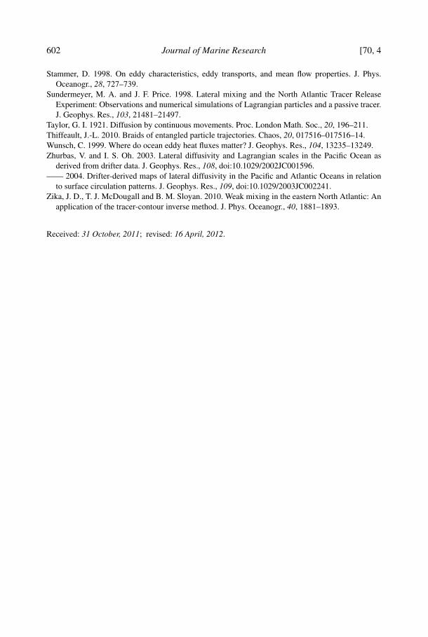
602 Journal of Marine Research [70, 4
Stammer, D. 1998. On eddy characteristics, eddy transports, and mean flow properties. J. Phys.Oceanogr., 28, 727–739.
Sundermeyer, M. A. and J. F. Price. 1998. Lateral mixing and the North Atlantic Tracer ReleaseExperiment: Observations and numerical simulations of Lagrangian particles and a passive tracer.J. Geophys. Res., 103, 21481–21497.
Taylor, G. I. 1921. Diffusion by continuous movements. Proc. London Math. Soc., 20, 196–211.Thiffeault, J.-L. 2010. Braids of entangled particle trajectories. Chaos, 20, 017516–017516–14.Wunsch, C. 1999. Where do ocean eddy heat fluxes matter? J. Geophys. Res., 104, 13235–13249.Zhurbas, V. and I. S. Oh. 2003. Lateral diffusivity and Lagrangian scales in the Pacific Ocean as
derived from drifter data. J. Geophys. Res., 108, doi:10.1029/2002JC001596.—— 2004. Drifter-derived maps of lateral diffusivity in the Pacific and Atlantic Oceans in relation
to surface circulation patterns. J. Geophys. Res., 109, doi:10.1029/2003JC002241.Zika, J. D., T. J. McDougall and B. M. Sloyan. 2010. Weak mixing in the eastern North Atlantic: An
application of the tracer-contour inverse method. J. Phys. Oceanogr., 40, 1881–1893.
Received: 31 October, 2011; revised: 16 April, 2012.
Related Documents