Published by the Institute of Electrical and Electronics Engineers, Inc. 551 ™ IEEE Recommended Practice for Calculating Short-Circuit Currents in Industrial and Commercial Power Systems IEEE Std 551 ™ -2006 Authorized licensed use limited to: UNIVERSIDADE DE SAO PAULO. Downloaded on September 14,2020 at 17:33:56 UTC from IEEE Xplore. Restrictions apply.

Welcome message from author
This document is posted to help you gain knowledge. Please leave a comment to let me know what you think about it! Share it to your friends and learn new things together.
Transcript

Published by theInstitute of Electrical and Electronics Engineers, Inc.
5 5 1™
IEEE Recommended Practice for
Calculating S h o rt - C i rc u i tC u r rents inIndustrial andC o m m e rcial P o w e r S y s t e m s
IEEE Std 551™-2006
Authorized licensed use limited to: UNIVERSIDADE DE SAO PAULO. Downloaded on September 14,2020 at 17:33:56 UTC from IEEE Xplore. Restrictions apply.

Authorized licensed use limited to: UNIVERSIDADE DE SAO PAULO. Downloaded on September 14,2020 at 17:33:56 UTC from IEEE Xplore. Restrictions apply.

Recognized as anAmerican National Standard (ANSI)
IEEE Std 551™-2006
IEEE Recommended Practice for Calculating Short-Circuit Currents in Industrial and Commercial Power Systems
Sponsor
Power Systems Engineering Committee
of the
IEEE Industry Applications Society
Approved 9 May 2006
IEEE-SA Standards Board
Approved 2 October 2006
American National Standards Institute
Authorized licensed use limited to: UNIVERSIDADE DE SAO PAULO. Downloaded on September 14,2020 at 17:33:56 UTC from IEEE Xplore. Restrictions apply.

The Institute of Electrical and Electronics Engineers, Inc.3 Park Avenue, New York, NY 10016-5997, USA
Copyright © 2006 by the Institute of Electrical and Electronics Engineers, Inc.All rights reserved. Published 17 November 2006. Printed in the United States of America.
IEEE is a registered trademark in the U.S. Patent & Trademark Office, owned by the Institute of Elec-trical and Electronics Engineers, Incorporated.
National Electrical Code and NEC are registered trademarks in the U.S. Patent & Trademark Office,owned by the National Fire Protection Association.
Print: ISBN 0-7381-4932-2 SH95520PDF: ISBN 0-7381-4933-0 SS95520
No part of this publication may be reproduced in any form, in an electronic retrieval system or other-wise, without the prior written permission of the publisher.
Abstract: This recommended practice provides short-circuit current information
including calculated short-circuit current duties for the application in industrial
plants and commercial buildings, at all power system voltages, of power system
equipment that senses, carries, or interrupts short-circuit currents. Equipment
coverage includes, but should not be limited to, protective device sensors such as
series trips and relays, passive equipment that may carry short-circuit current such
as bus, cable, reactors and transformers as well as interrupters such as circuit
breakers and fuses.
Keywords: available fault current, circuit breaker, circuit breaker applications,
fuse, power system voltage, reactors, short-circuit applications guides, short-
circuit duties
Authorized licensed use limited to: UNIVERSIDADE DE SAO PAULO. Downloaded on September 14,2020 at 17:33:56 UTC from IEEE Xplore. Restrictions apply.

IEEE Standards documents are developed within the IEEE Societies and the Standards Coordinating Committees
of the IEEE Standards Association (IEEE-SA) Standards Board. The IEEE develops its standards through a
consensus development process, approved by the American National Standards Institute, which brings together
volunteers representing varied viewpoints and interests to achieve the final product. Volunteers are not necessarily
members of the Institute and serve without compensation. While the IEEE administers the process and establishes
rules to promote fairness in the consensus development process, the IEEE does not independently evaluate, test, or
verify the accuracy of any of the information contained in its standards.
Use of an IEEE Standard is wholly voluntary. The IEEE disclaims liability for any personal injury, property or
other damage, of any nature whatsoever, whether special, indirect, consequential, or compensatory, directly or
indirectly resulting from the publication, use of, or reliance upon this, or any other IEEE Standard document.
The IEEE does not warrant or represent the accuracy or content of the material contained herein, and expressly
disclaims any express or implied warranty, including any implied warranty of merchantability or fitness for a spe-
cific purpose, or that the use of the material contained herein is free from patent infringement. IEEE Standards
documents are supplied “AS IS.”
The existence of an IEEE Standard does not imply that there are no other ways to produce, test, measure, purchase,
market, or provide other goods and services related to the scope of the IEEE Standard. Furthermore, the viewpoint
expressed at the time a standard is approved and issued is subject to change brought about through developments
in the state of the art and comments received from users of the standard. Every IEEE Standard is subjected to
review at least every five years for revision or reaffirmation. When a document is more than five years old and has
not been reaffirmed, it is reasonable to conclude that its contents, although still of some value, do not wholly
reflect the present state of the art. Users are cautioned to check to determine that they have the latest edition of any
IEEE Standard.
In publishing and making this document available, the IEEE is not suggesting or rendering professional or other
services for, or on behalf of, any person or entity. Nor is the IEEE undertaking to perform any duty owed by any
other person or entity to another. Any person utilizing this, and any other IEEE Standards document, should rely
upon the advice of a competent professional in determining the exercise of reasonable care in any given
circumstances.
Interpretations: Occasionally questions may arise regarding the meaning of portions of standards as they relate to
specific applications. When the need for interpretations is brought to the attention of IEEE, the Institute will initiate
action to prepare appropriate responses. Since IEEE Standards represent a consensus of concerned interests, it is
important to ensure that any interpretation has also received the concurrence of a balance of interests. For this
reason, IEEE and the members of its societies and Standards Coordinating Committees are not able to provide an
instant response to interpretation requests except in those cases where the matter has previously received formal
consideration. At lectures, symposia, seminars, or educational courses, an individual presenting information on
IEEE standards shall make it clear that his or her views should be considered the personal views of that individual
rather than the formal position, explanation, or interpretation of the IEEE.
Comments for revision of IEEE Standards are welcome from any interested party, regardless of membership
affiliation with IEEE. Suggestions for changes in documents should be in the form of a proposed change of text,
together with appropriate supporting comments. Comments on standards and requests for interpretations should be
addressed to:
Secretary, IEEE-SA Standards Board
445 Hoes Lane
Piscataway, NJ 08854
USA
Authorization to photocopy portions of any individual standard for internal or personal use is granted by the
Institute of Electrical and Electronics Engineers, Inc., provided that the appropriate fee is paid to Copyright
Clearance Center. To arrange for payment of licensing fee, please contact Copyright Clearance Center, Customer
Service, 222 Rosewood Drive, Danvers, MA 01923 USA; +1 978 750 8400. Permission to photocopy portions of
any individual standard for educational classroom use can also be obtained through the Copyright
Clearance Center.
Authorized licensed use limited to: UNIVERSIDADE DE SAO PAULO. Downloaded on September 14,2020 at 17:33:56 UTC from IEEE Xplore. Restrictions apply.

iv Copyright © 2006 IEEE. All rights reserved.
Introduction
This recommended practice is intended as a practical, general treatise for engineers on the
subject of ac short-circuit currents in electrical power systems. The focus of this standard
is the understanding and application of analytical techniques of short-circuit analysis in
industrial and commercial power systems. However, the same engineering principles
apply to all electrical power systems, including utilities and systems other than 60 Hz.
More than any other book in the IEEE Color Book® series, the “Violet Book” covers the
basics of short-circuit currents. To help the reader, the same one-line diagram that is used
in several of the other color books is used in sample calculations. Items covered in the
Violet Book that are not covered in the other color book chapters on short-circuit currents
are the contributions of regenerative SCR drives and capacitors to faults. The reference
data chapter in this recommended practice is quite extensive and should be very useful for
any type of power system analysis.
Notice to users
Errata
Errata, if any, for this and all other standards can be accessed at the following URL: http:/
/standards.ieee.org/reading/ieee/updates/errata/index.html. Users are encouraged to check
this URL for errata periodically.
Interpretations
Current interpretations can be accessed at the following URL: http://standards.ieee.org/
reading/ieee/interp/index.html.
Patents
Attention is called to the possibility that implementation of this standard may require use
of subject matter covered by patent rights. By publication of this standard, no position is
taken with respect to the existence or validity of any patent rights in connection therewith.
The IEEE shall not be responsible for identifying patents or patent applications for which
a license may be required to implement an IEEE standard or for conducting inquiries into
the legal validity or scope of those patents that are brought to its attention.
This introduction is not part of IEEE Std 551-2006, IEEE Recommended Practice for CalculatingShort-Circuit Currents in Industrial and Commercial Power Systems.
Authorized licensed use limited to: UNIVERSIDADE DE SAO PAULO. Downloaded on September 14,2020 at 17:33:56 UTC from IEEE Xplore. Restrictions apply.

Copyright © 2006 IEEE. All rights reserved. v
Participants
To many members of the working group who wrote and developed the chapters in this rec-
ommended practice, the Violet Book has been a labor of love and a long time coming.
Over the years, some members have come and gone, but their efforts are sincerely appre-
ciated. To all the members past and present, many thanks for your excellent contributions.
The following working group members of the Power System Analysis Subcommittee of
the Power Systems Engineering Committee of the IEEE Industry Applications Society
and some non-members contributed to the existence of the Violet Book:
Jason MacDowell, Chair (2003-2006)
S. Mark Halpin, Chair (2000-2003)
L. Guy Jackson, Chair (1998-2000)
Conrad R. St. Pierre, Chair (1989-1998)
Walter C. Huening, Chair (1965-1989)
Chapter authors:
Chapter reviewers/contributors
Chet E. Davis
Richard L. Doughty
M. Shan Griffith
William R. Haack
Timothy T. Ho
Walter C. Huening
Douglas M. Kaarcher
Bal K. Mathur
Elliot Rappaport
Alfred A. Regotti
Anthony J. Rodolakis
Michael A. Slonim
David H. Smith
Conrad R. St. Pierre
Neville A. Williams
Michael Aimone
Jack Alacchi
William E. Anderson
R. Gene Baggs
Roy D. Boyer
Reuben Burch
Bernard W. Cable
W. Fred Carden, Jr.
Hari P. S. Cheema
Norman R. Conte
Chet E. Davis
Robert J. Deaton
Phillip C. Doolittle
Richard L. Doughty
James W. Feltes
Ken Fleischer
Pradit Fuangfoo
M. Shan Griffith
William R. Haack
William Hall
S. Mark Halpin
Robert C. Hay, Sr.
Timothy T. Ho
Robert G. Hoerauf
Walter C. Huening
Guy Jackson
Douglas M. Kaercher
Alton (Gene) Knight
John A. Kroiss
Wei-Jen Lee
Jason MacDowell
Bal K. Mathur
Richard H. McFadden
Steve Miller
William J. Moylan
Russell O. Olson
Laurie Oppel
Norman Peach
David J. Podobinski
Louie J. Powell
Ralph C. Prichard
Elliot Rappaport
Alfred A. Regotti
Michael L. Reichard
Anthony J. Rodolakis
Willaim C. Roettger
Vincent Saporita
George Schliapnikoff
David D. Shipp
Farrokh Shokooh
Charles A. Shrive
Michael A. Slonim
David H. Smith
J. R. Smith
Gary T. Smullin
Conrad R. St. Pierre
Peter Sutherland
George A. Terry
Lynn M. Tooman
S. I. Venugopalan
Donald A. Voltz
Claus Wiig
Neville A. Williams
Authorized licensed use limited to: UNIVERSIDADE DE SAO PAULO. Downloaded on September 14,2020 at 17:33:56 UTC from IEEE Xplore. Restrictions apply.

vi Copyright © 2006 IEEE. All rights reserved.
Acknowledgment
Appreciation is expressed to the following companies and organizations for contributing
the time and in some cases expenses of the working group members and their support help
to make possible the development of this text.
AVCA Corporation
Brown & Root, Inc.
CYME International, Inc.
Electrical System Analysis
General Electric Company
ICF Kaiser Engineers
Jackson & Associates
Power Technologies, Inc.
The following members of the individual balloting committee voted on this recommended
practice. Balloters may have voted for approval, disapproval, or abstention.
David Aho
Paul Anderson
Dick Becker
Behdad Biglar
Stuart Bouchey
Reuben Burch
Donald Colaberardino
Stephen Conrad
Stephen Dare
Robert Deaton
Guru Dutt Dhingra
Matthew Dozier
Donald Dunn
Thomas Ernst
Dan Evans
Jay Fischer
Marcel Fortin
Carl Fredericks
Edgar Galyon
George Gregory
Randall Groves
Paul Hamer
Robert Hoerauf
Ronald Hotchkiss
Darin Hucul
Walter C. Huening
Robert Ingham
David Jackson
L. Guy Jackson
Brian Johnson
Don Koval
Blane Leuschner
Jason Lin
Gregory Luri
William Majeski
L. Bruce McClung
Jeff McElray
Mark McGranaghan
James Michalec
Gary Michel
T. David Mills
William Moylan
Daniel Neeser
Kenneth Nicholson
Lorraine Padden
Gene Poletto
Louie Powell
Madan Rana
James Ruggieri
Donald Ruthman
Vincent Saporita
Robert Schuerger
Michael Shirven
H. Jin Sim
Harinderpal Singh
David Singleton
Robert Smith
Gary Smullin
Jane Ann Verner
S. Frank Waterer
Zhenxue Xu
Authorized licensed use limited to: UNIVERSIDADE DE SAO PAULO. Downloaded on September 14,2020 at 17:33:56 UTC from IEEE Xplore. Restrictions apply.

Copyright © 2006 IEEE. All rights reserved. vii
The final conditions for approval of this standard were met on 9 May 2006. This standard
was conditionally approved by the IEEE-SA Standards Board on 30 March 2006, with the
following membership:
Steve M. Mills, ChairRichard H. Hulett, Vice Chair
Don Wright, Past ChairJudith Gorman, Secretary
*Member Emeritus
Also included are the following nonvoting IEEE-SA Standards Board liaisons:
Satish K. Aggarwal, NRC RepresentativeRichard DeBlasio, DOE RepresentativeAlan H. Cookson, NIST Representative
Michael FisherIEEE Standards Program Manager, Document Development
Mark D. BowmanDennis B. BrophyWilliam R. GoldbachArnold M. GreenspanRobert M. GrowJoanna N. GueninJulian Forster*Mark S. Halpin
Kenneth S. HanusWilliam B. HopfJoseph L. Koepfinger*David J. LawDaleep C. MohlaT. W. OlsenGlenn ParsonsRonald C. PetersenTom A. Prevost
Greg RattaRobby RobsonAnne-Marie SahazizianVirginia C. SulzbergerMalcolm V. ThadenRichard L. TownsendWalter WeigelHoward L. Wolfman
Authorized licensed use limited to: UNIVERSIDADE DE SAO PAULO. Downloaded on September 14,2020 at 17:33:56 UTC from IEEE Xplore. Restrictions apply.

viii Copyright © 2006 IEEE. All rights reserved.
Contents
Chapter 1Introduction ........................................................................................................................ 1
1.1 Scope............................................................................................................... 1
1.2 Definitions ...................................................................................................... 2
1.3 Acronyms and abbreviations .......................................................................... 8
1.4 Bibliography ................................................................................................. 10
1.5 Manufacturers’ data sources ......................................................................... 11
Chapter 2
Description of a short-circuit current ............................................................................... 13
2.1 Introduction................................................................................................... 13
2.2 Available short-circuit .................................................................................. 13
2.3 Symmetrical and asymmetrical currents....................................................... 14
2.4 Short-circuit calculations .............................................................................. 17
2.5 Total short-circuit current ............................................................................. 20
2.6 Why short-circuit currents are asymmetrical................................................ 22
2.7 DC component of short-circuit currents ....................................................... 22
2.8 Significance of current asymmetry ............................................................... 22
2.9 The application of current asymmetry information ...................................... 23
2.10 Maximum peak current ................................................................................. 24
2.11 Types of faults .............................................................................................. 31
2.12 Arc resistance................................................................................................ 32
2.13 Bibliography ................................................................................................. 34
Chapter 3
Calculating techniques ..................................................................................................... 37
3.1 Introduction.................................................................................................. 37
3.2 Fundamental principles................................................................................ 37
3.3 Short-circuit calculation procedure.............................................................. 42
3.4 One-line diagram ......................................................................................... 43
3.5 Per-unit and ohmic manipulations ............................................................... 50
3.6 Network theorems and calculation techniques ............................................ 52
3.7 Extending a three-phase short-circuit calculation procedures program
to calculate short-circuit currents for single-phase branches....................... 67
3.8 Representing transformers with non-base voltages ..................................... 69
3.9 Specific time period and variations on fault calculations ............................ 78
3.10 Determination of X/R ratios for ANSI fault calculations............................. 81
3.11 Three winding transformers......................................................................... 81
3.12 Duplex reactor ............................................................................................. 82
3.13 Significant cable lengths.............................................................................. 83
3.14 Equivalent circuits ....................................................................................... 84
3.15 Zero sequence line representation ............................................................... 85
3.16 Equipment data required for short-circuit calculations ............................... 86
3.17 Bibliography ................................................................................................ 94
Authorized licensed use limited to: UNIVERSIDADE DE SAO PAULO. Downloaded on September 14,2020 at 17:33:56 UTC from IEEE Xplore. Restrictions apply.

Copyright © 2006 IEEE. All rights reserved. ix
Chapter 4
Calculating short-circuit currents for systems without ac delay....................................... 95
4.1 Introduction................................................................................................... 95
4.2 Purpose.......................................................................................................... 95
4.3 ANSI guidelines............................................................................................ 96
4.4 Fault calculations .......................................................................................... 97
4.5 Sample calculations ...................................................................................... 98
4.6 Sample computer printout........................................................................... 103
4.7 Conclusions................................................................................................. 113
4.8 Bibliography ............................................................................................... 114
Chapter 5
Calculating ac short-circuit currents for systems with contributions from
synchronous machines ................................................................................................... 115
5.1 Introduction................................................................................................. 115
5.2 Purpose........................................................................................................ 115
5.3 ANSI guidelines.......................................................................................... 115
5.4 Fault calculations ........................................................................................ 116
5.5 Nature of synchronous machine contributions ........................................... 116
5.6 Synchronous machine reactances ............................................................... 119
5.7 One-line diagram data................................................................................. 121
5.8 Sample calculations .................................................................................... 121
5.9 Sample computer printout........................................................................... 123
5.10 Sample computer printout for larger system calculations .......................... 124
5.11 Conclusions................................................................................................. 126
5.12 Bibliography ............................................................................................... 126
Chapter 6
Calculating ac short-circuit currents for systems with contributions from
induction motors ............................................................................................................ 127
6.1 Introduction................................................................................................. 127
6.2 Purpose........................................................................................................ 127
6.3 ANSI guidelines.......................................................................................... 127
6.4 Fault calculations ........................................................................................ 129
6.5 Nature of induction motor contributions .................................................... 129
6.6 Large induction motors with prolonged contributions ............................... 132
6.7 Data accuracy.............................................................................................. 133
6.8 Details of induction motor contribution calculations according to
ANSI standard application guides............................................................... 133
6.9 Recommended practice based on ANSI-approved standards for representing
induction motors in multivoltage system studies ........................................ 135
6.10 One-line diagram data................................................................................. 137
6.11 Sample calculations .................................................................................... 138
6.12 Sample computer printout........................................................................... 142
6.13 Bibliography ............................................................................................... 145
Authorized licensed use limited to: UNIVERSIDADE DE SAO PAULO. Downloaded on September 14,2020 at 17:33:56 UTC from IEEE Xplore. Restrictions apply.
x Copyright © 2006 IEEE. All rights reserved.
Chapter 7
Capacitor contributions to short-circuit currents ........................................................... 147
7.1 Introduction................................................................................................. 147
7.2 Capacitor discharge current ........................................................................ 147
7.3 Transient simulations .................................................................................. 149
7.4 Summary..................................................................................................... 165
7.5 Bibliography ............................................................................................... 165
Chapter 8
Static converter contributions to short-circuit currents.................................................. 167
8.1 Introduction................................................................................................. 167
8.2 Definitions of converter types..................................................................... 167
8.3 Converter circuits and their equivalent parameters .................................... 168
8.4 Short-circuit current contribution from the dc system to an
ac short circuit............................................................................................. 170
8.5 Analysis of converter dc faults ................................................................... 176
8.6 Short circuit between the converter dc terminals........................................ 177
8.7 Arc-back short circuits................................................................................ 187
8.8 Examples..................................................................................................... 191
8.9 Conclusions................................................................................................. 197
8.10 Bibliography ............................................................................................... 197
Chapter 9
Calculating ac short-circuit currents in accordance with ANSI-approved standards .... 199
9.1 Introduction................................................................................................. 199
9.2 Basic assumptions and system modeling.................................................... 199
9.3 ANSI recommended practice for ac decrement modeling.......................... 200
9.4 ANSI practice for dc decrement modeling ................................................. 204
9.5 ANSI-conformable fault calculations ......................................................... 212
9.6 ANSI-approved standards and interrupting duties...................................... 214
9.7 One-line diagram layout and data ............................................................... 216
9.8 First cycle duty sample calculations ........................................................... 219
9.9 Interrupting duty sample calculations......................................................... 223
9.10 Applying ANSI calculations to non-60 Hz systems ................................... 228
9.11 Normative references .................................................................................. 229
9.12 Bibliography ............................................................................................... 230
Chapter 10
Application of short-circuit interrupting equipment ...................................................... 231
10.1 Introduction................................................................................................. 231
10.2 Purpose........................................................................................................ 231
10.3 Application considerations ......................................................................... 231
10.4 Equipment data ........................................................................................... 233
10.5 Fully rated systems ..................................................................................... 234
10.6 Low voltage series rated equipment ........................................................... 234
10.7 Low voltage circuit breaker short-circuit capabilities less than rating ....... 235
10.8 Equipment checklist for short-circuit currents evaluation .......................... 236
Authorized licensed use limited to: UNIVERSIDADE DE SAO PAULO. Downloaded on September 14,2020 at 17:33:56 UTC from IEEE Xplore. Restrictions apply.

Copyright © 2006 IEEE. All rights reserved. xi
10.9 Equipment phase duty calculations ........................................................... 237
10.10 Equipment ground fault duty calculations................................................. 245
10.11 Capacitor Switching .................................................................................. 245
10.12 Normative references ................................................................................ 246
Chapter 11
Unbalanced short-circuit currents .................................................................................. 249
11.1 Introduction ............................................................................................... 249
11.2 Purpose ...................................................................................................... 249
11.3 ANSI guidelines ........................................................................................ 250
11.4 Procedure ................................................................................................... 251
11.5 Connection of sequence networks ............................................................. 257
11.6 Sample calculations ................................................................................... 258
11.7 Conclusions ............................................................................................... 271
11.8 Bibliography .............................................................................................. 271
Chapter 12
Short-circuit calculations unser international standards ................................................ 273
12.1 Introduction ............................................................................................... 273
12.2 System modeling and methodologies........................................................ 273
12.3 Voltage factors .......................................................................................... 275
12.4 Short circuit currents per IEC 60909......................................................... 275
12.5 Short circuits “far from generator”............................................................ 276
12.6 Short circuits “near generator” .................................................................. 281
12.7 Influence of the motors.............................................................................. 290
12.8 Fault calculations in complex systems ...................................................... 292
12.9 Comparing the ANSI-approved standards with IEC 909.......................... 292
12.10 Sample calculations................................................................................... 293
12.11 Normative references ................................................................................ 299
12.12 Bibliography.............................................................................................. 300
Authorized licensed use limited to: UNIVERSIDADE DE SAO PAULO. Downloaded on September 14,2020 at 17:33:56 UTC from IEEE Xplore. Restrictions apply.

Authorized licensed use limited to: UNIVERSIDADE DE SAO PAULO. Downloaded on September 14,2020 at 17:33:56 UTC from IEEE Xplore. Restrictions apply.

Copyright © 2006 IEEE. All rights reserved. 1
IEEE Recommended Practice for Calculating Short-CircuitCurrents in Industrial and Commercial Power Systems
Chapter 1Introduction
1.1 Scope
Electric power systems in industrial plants and commercial and institutional buildings are
designed to serve loads in a safe and reliable manner. One of the major considerations in
the design of a power system is adequate control of short circuits or faults as they are
commonly called. Uncontrolled short-circuits can cause service outage with
accompanying production downtime and associated inconvenience, interruption of
essential facilities or vital services, extensive equipment damage, personnel injury or
fatality, and possible fire damage.
Short-circuits are caused by faults in the insulation of a circuit, and in many cases an arc
ensues at the point of the fault. Such an arc may be destructive and may constitute a fire
hazard. Prolonged duration of arcs, in addition to the heat released, may result in transient
overvoltages that may endanger the insulation of equipment in other parts of the system.
Clearly, the fault must be quickly removed from the power system, and this is the job of
the circuit protective devices—the circuit breakers and fusible switches.
A short-circuit current generates heat that is proportional to the square of the current
magnitude, I2R. The large amount of heat generated by a short-circuit current may damage
the insulation of rotating machinery and apparatus that is connected into the faulted
system, including cables, transformers, switches, and circuit breakers. The most
immediate danger involved in the heat generated by short-circuit currents is permanent
destruction of insulation. This may be followed by actual fusion of the conducting circuit,
with resultant additional arcing faults.
Authorized licensed use limited to: UNIVERSIDADE DE SAO PAULO. Downloaded on September 14,2020 at 17:33:56 UTC from IEEE Xplore. Restrictions apply.

IEEEStd 551-2006 CHAPTER 1
2 Copyright © 2006 IEEE. All rights reserved.
The heat that is generated by high short-circuit currents tends not only to impair insulating
materials to the point of permanent destruction, but also exerts harmful effects upon the
contact members in interrupting devices.
The small area common between two contact members that are in engagement depends
mainly upon the hardness of the contact material and upon the amount of pressure by
which they are kept in engagement. Owing to the concentration of the flow of current at
the points of contact engagement, the temperatures of these points reached at the times of
peak current are very high. As a result of these high spot temperatures, the material of
which the contact members are made may soften. If, however, the contact material is
caused to melt by excessive I2R losses, there is an imminent danger of welding the
contacts together rendering it impossible to separate the contact members when the switch
or circuit breaker is called upon to open the circuit. Since it requires very little time to
establish thermal equilibrium at the small points of contact engagement, the temperature at
these points depends more upon the peak current than upon the rms current. If the peak
current is sufficient to cause the contact material to melt, resolidification may occur
immediately upon decrease of the current from its peak value.
Other important effects of short-circuit currents are the strong electromagnetic forces of
attraction and repulsion to which the conductors are subjected when short-circuit currents
are present. These forces are proportional to the square of the current and may subject any
rotating machinery, transmission, and switching equipment to severe mechanical stresses
and strains. The strong electromagnetic forces that high short-circuit currents exert upon
equipment can cause deformation in rotational machines, transformer windings, and
equipment bus bars, which may fail at a future time. Deformation in breakers and switches
will cause alignment and interruption difficulties.
Modern interconnected systems involve the operation in parallel of large numbers of
synchronous machines, and the stability of such an interconnected system may be greatly
impaired if a short-circuit in any part of the system is allowed to prevail. The stability of a
system requires short fault clearing times and can be more limiting than the longer time
considerations imposed by thermal or mechanical effects on the equipment.
1.2 Definitions
For the purpose of this document, the following terms and definitions apply. The Authori-tative Dictionary of IEEE Standards Terms [B3]1 should be referenced for terms not
defined in this clause.
1.2.1 30 cycle time: The time interval between the time when the actuating quantity of the
release circuit reaches the operating value, and the approximate time when the primary
arcing contacts have parted. The time period considers the ac decaying component of a
fault current to be negligible.
1The numbers in brackets correspond to those of the bibliography in 1.4.
Authorized licensed use limited to: UNIVERSIDADE DE SAO PAULO. Downloaded on September 14,2020 at 17:33:56 UTC from IEEE Xplore. Restrictions apply.

IEEEINTRODUCTION Std 551-2006
Copyright © 2006 IEEE. All rights reserved. 3
1.2.2 arcing time: The interval of time between the instant of the first initiation of the arc
and the instant of final arc extinction in all poles.
1.2.3 armature: The main current carrying winding of a machine, usually the stator.
1.2.4 armature resistance: Ra—The direct current armature resistance. This is
determined from a dc resistance measurement. The approximate effective ac resistance is
1.2Ra.
1.2.5 asymmetrical current: The combination of the symmetrical component and the
direct current component of the current.
1.2.6 available current: The current that would flow if each pole of the breaking device
under consideration were replaced by a link of negligible impedance without any change
of the circuit or the supply.
1.2.7 breaking current: The current in a pole of a switching device at the instant of the
arc initiation. Better known as interrupting current.
1.2.8 circuit breaker: A switching device capable of making, carrying, and breaking
currents under normal circuit conditions and also making, carrying for a specified time,
and breaking currents under specified abnormal conditions such as those of short circuit.
1.2.9 clearing time: The total time between the beginning of specified overcurrent and the
final interruption of the circuit at rated voltage. In regard to fuses, it is the sum of the
minimum melting time of a fuse plus tolerance and the arcing time. In regard to breakers
under 1000 V, it is the sum of the sensor time, plus opening time and the arcing time. For
breakers rated above 1000 V, it is the sum of the minimum relay time (usually 1/2 cycle),
plus contact parting time and the arcing time. Sometimes referred to as total clearing timeor interrupting time.
1.2.10 close and latch: The capability of a switching device to close (allow current flow)
and immediately thereafter latch (remain closed) and conduct a specified current through
the device under specified conditions.
1.2.10.1 close and latch duty: The maximum rms value of calculated short-circuit current
for medium- and high-voltage circuit breakers during the first cycle with any applicable
multipliers for fault current X/R ratio. Often the close and latching duty calculation is sim-
plified by applying a 1.6 factor to the calculated breaker first cycle symmetrical ac rms
short-circuit current. Also called first cycle duty (formerly, momentary duty).
1.2.10.2 close and latch rating: The maximum current capability of a medium or
high-voltage circuit breaker to close and immediately thereafter latching closed for
normal-frequency making current. The close and latching rating is 1.6 times the breaker
rated maximum symmetrical interrupting current in ac rms amperes or a peak current that
is 2.7 times ac rms rated maximum symmetrical interrupting current. Also called first
cycle rating (formerly, momentary rating).
Authorized licensed use limited to: UNIVERSIDADE DE SAO PAULO. Downloaded on September 14,2020 at 17:33:56 UTC from IEEE Xplore. Restrictions apply.
IEEEStd 551-2006 CHAPTER 1
4 Copyright © 2006 IEEE. All rights reserved.
1.2.11 contact parting time: The interval between the time when the actuating quantity in
the release circuit reaches the value causing actuation of the release and the instant when
the primary arcing contacts have parted in all poles. Contact parting time is the numerical
sum of release delay and opening time.
1.2.12 crest current: The highest instantaneous current during a period. Syn: peak
current.
1.2.13 direct axis: The machine axis that represents a plane of symmetry in line with the
no-load field winding.
1.2.14 direct axis subtransient reactance: X"dv (saturated, rated voltage) is the apparent
reactance of the stator winding at the instant short-circuit occurs with the machine at rated
voltage, no load. This reactance determines the current flow during the first few cycles
after short-circuit.
1.2.15 direct axis subtransient reactance: X"di (unsaturated, rated current) is the
reactance that is determined from the ratio of an initial reduced voltage open circuit
condition and the currents from a three-phase fault at the machine terminals at rated
frequency. The initial open-circuit voltage is adjusted so that rated current is obtained. The
impedance is determined from the currents during the first few cycles.
1.2.16 direct axis transient reactance: X'dv (saturated, rated voltage) is the apparent
reactance of the stator winding several cycles after initiation of the fault with the machine
at rated voltage, no load. The time period for which the reactance may be considered X'dv
can be up to a half (1/2) second or longer, depending upon the design of the machine and
is determined by the machine direct-axis transient time constant.
1.2.17 direct axis transient reactance: X'di (unsaturated, rated current) is the reactance
that is determined from the ratio of an initial reduced voltage open circuit condition and
the currents from a three-phase fault at the machine terminals at rated frequency. The
initial open-circuit voltage is adjusted so that rated current is obtained. The initial high
decrement currents during the first few cycles are neglected.
1.2.18 fault: A current that flows from one conductor to ground or to another conductor
owing to an abnormal connection (including an arc) between the two. Syn: short circuit.
1.2.19 fault point angle: The calculated fault point angle (Tan–1(X/R ratio) using complex
(R + jX) reactance and resistance networks for the X/R ratio.
1.2.20 fault point X/R: The calculated fault point X/R ratio using separate reactance and
resistance networks.
1.2.21 field: The exciting or magnetizing winding of a machine.
1.2.22 first cycle duty: The maximum value of calculated short-circuit current for the first
cycle with any applicable multipliers for fault current X/R ratio.
Authorized licensed use limited to: UNIVERSIDADE DE SAO PAULO. Downloaded on September 14,2020 at 17:33:56 UTC from IEEE Xplore. Restrictions apply.
IEEEINTRODUCTION Std 551-2006
Copyright © 2006 IEEE. All rights reserved. 5
1.2.23 first cycle rating: The maximum current capability of a piece of equipment during
the first cycle of a fault.
1.2.24 frequency: The rated frequency of a circuit.
1.2.25 fuse: A device that protects a circuit by melting open its current-carrying element
when an overcurrent or short-circuit current passes through it.
1.2.26 high voltage: Circuit voltages over nominal 34.5 kV.
NOTE—ANSI standards are not unanimous in establishing the threshold of “high-voltage.”2
1.2.27 impedance: The vector sum of resistance and reactance in an ac circuit.
1.2.28 interrupting current: The current in a pole of a switching device at the instant of
the arc initiation. Sometime referred to as breaking current.
1.2.29 interrupting time: The interval between the time when the actuating device “sees”
or responds to a operating value, the opening time and arcing time. Sometimes referred to
as total break time or clearing time.
1.2.30 low voltage: Circuit voltage under 1000 V.
1.2.31 maximum rated voltage: The upper operating voltage limit for a device.
1.2.32 medium voltage: Circuit voltage greater than 1000 V up to and including 34.5 kV.
NOTE—ANSI standards are not unanimous in establishing the threshold of “high-voltage.”
1.2.33 minimum rated voltage: The lower operating voltage limit for a device where the
rated interrupting current is a maximum. Operating breakers at voltages lower than
minimum rated voltage restricts the interrupting current to maximum rated interrupting
current.
1.2.34 momentary current rating: The maximum rms current measured at the major
peak of the first cycle, which the device or assembly is required to carry. Momentary
rating was used on medium- and high-voltage breakers manufactured before 1965. See
presently used terminology of close and latch rating.
1.2.35 momentary current duty: See presently used terminology of close and latch
duty. Used for medium- and high-voltage breaker duty calculations for breakers
manufactured before 1965.
1.2.36 negative sequence: A set of symmetrical components that have the angular phase
lag from the first member of the set to the second and every other member of the set equal
to the characteristic angular phase difference and rotating in the reverse direction of the
2Notes in text, tables, and figures are given for information only and do not contain requirements needed toimplement the standard.
Authorized licensed use limited to: UNIVERSIDADE DE SAO PAULO. Downloaded on September 14,2020 at 17:33:56 UTC from IEEE Xplore. Restrictions apply.
IEEEStd 551-2006 CHAPTER 1
6 Copyright © 2006 IEEE. All rights reserved.
original vectors. For a three-phase system, the angular different is 120 degrees. See also:symmetrical components.
1.2.37 negative sequence reactance: X2v (saturated, rated voltage). The rated current
value of negative-sequence reactance is the value obtained from a test with a fundamental
negative-sequence current equal to rated armature current (of the machine). The rated
voltage value of negative-sequence reactance is the value obtained from a line-to-line
short-circuit test at two terminals of the machine at rated speed, applied from no load at
rated voltage, the resulting value being corrected when necessary for the effect of
harmonic components in the current.
1.2.38 offset current: A current waveform whose baseline is offset from the ac
symmetrical current zero axis.
1.2.39 opening time: The time interval between the time when the actuating quantity of
the release circuit reaches the operating value, and the instant when the primary arcing
contacts have parted. The opening time includes the operating time of an auxiliary relay in
the release circuit when such a relay is required and supplied as part of the switching
device.
1.2.40 peak current: The highest instantaneous current during a period.
1.2.41 positive sequence: A set of symmetrical components that have the angular phase
lag from the first member of the set to the second and every other member of the set equal
to the characteristic angular phase difference and rotating in the same phase sequence of
the original vectors. For a three-phase system, the angular different is 120 degrees. Seealso: symmetrical components.
1.2.42 positive sequence machine resistance: R1 is that value of rated frequency
armature resistance that, when multiplied by the square of the rated positive-sequence
armature current and by the number of phases, is equal to the sum of the copper loss in the
armature and the load loss resulting from the flow of that current. This is NOT the
resistance to be used for the machine in short-circuit calculations.
1.2.43 quadrature axis: The machine axis that represents a plane of symmetry in the field
that produces no magnetization. This axis is 90 degrees ahead of the direct axis.
1.2.44 quadrature axis subtransient reactance: X"qv (saturated, rated voltage) same as
X"dv except in quadrature axis.
1.2.45 quadrature axis subtransient reactance: X"qi (unsaturated, rated current) same as
X"di except in quadrature axis.
1.2.46 quadrature axis transient reactance: Xq (unsaturated, rated current) is the ratio of
reactive armature voltage to quadrature-axis armature current at rated frequency and
voltage.
Authorized licensed use limited to: UNIVERSIDADE DE SAO PAULO. Downloaded on September 14,2020 at 17:33:56 UTC from IEEE Xplore. Restrictions apply.

IEEEINTRODUCTION Std 551-2006
Copyright © 2006 IEEE. All rights reserved. 7
1.2.47 quadrature axis transient reactance: X'qv (saturated, rated voltage) same as X'dv
except in q quadrature axis.
1.2.48 quadrature axis transient reactance: X'qi (unsaturated, rated voltage) same as X'di
except in quadrature axis.
1.2.49 rating: The designated limit(s) of the operating characteristic(s) of a device. This
data is usually on the device nameplate.
1.2.50 rms: The square root of the average value of the square of the voltage or current
taken throughout one period. In this text, rms will be considered total rms unless otherwise
noted.
1.2.51 rms ac: The square root of the average value of the square of the ac voltage or
current taken throughout one period.
1.2.52 rms, single cycle: See: single-cycle rms.
1.2.53 rms, total: See: total rms.
1.2.54 rotor: The rotating member of a machine.
1.2.55 short circuit: An abnormal connection (including arc) of relative low impedance,
whether made accidentally or intentionally, between two points of different potentials.
Syn: fault.
1.2.56 short-circuit duty: The maximum value of calculated short-circuit current for
either first cycle current or interrupting current with any applicable multipliers for fault
current X/R ratio or decrement.
1.2.57 single-cycle rms: The square root of the average value of the square of the ac
voltage or current taken throughout one ac cycle.
1.2.58 stator: The stationary member of a machine.
1.2.59 symmetrical: That portion of the total current that, when viewed as a waveform,
has equal positive and negative values over time such as is exhibited by a pure single-
frequency sinusoidal waveform
1.2.60 symmetrical components: A symmetrical set of three vectors used to
mathematically represent an unsymmetrical set of three-phase voltages or currents. In a
three-phase system, one set of three equal magnitude vectors displaced from each other by
120 degrees in the same sequence as the original set of unsymmetrical vectors. This set of
vectors is called the positive sequence component. A second set of three equal magnitude
vectors displaced from each other by 120 degrees in the reverse sequence as the original
set of unsymmetrical vectors. This set of vectors is called the negative sequence
component. A third set of three equal magnitude vectors displaced from each other by
0 degrees. This set of vectors is called the zero sequence component.
Authorized licensed use limited to: UNIVERSIDADE DE SAO PAULO. Downloaded on September 14,2020 at 17:33:56 UTC from IEEE Xplore. Restrictions apply.

IEEEStd 551-2006 CHAPTER 1
8 Copyright © 2006 IEEE. All rights reserved.
1.2.61 synchronous reactance: Direct axis Xd (unsaturated, rated current) is the self
reactance of the armature winding to the steady-state balanced three-phase positive-
sequence current at rated frequency and voltage in the direct axis. It is determined from an
initial open-circuit voltage and a sustained short circuit on the a synchronous machine
terminals.
1.2.62 three-phase open circuit time constant: Ta3 is the time constant representing the
decay of the machine currents to a suddenly applied three-phase short-circuit to the
terminals of a machine.
1.2.63 total break time: The interval between the time when the actuating quantity of the
release circuit reaches the operating value, the switching device being in a closed position,
and the instant of arc extinction on the primary arcing contacts. Total break time is equal
to the sum of the opening time and arcing time. Better known as interrupting time.
1.2.64 total clearing time: See: clearing time or interrupting time.
1.2.65 total rms: The square root of the average value of the square of the ac and dc
voltage or current taken throughout one period.
1.2.66 voltage, high: See: high voltage.
1.2.67 voltage, low: See: low voltage.
1.2.68 voltage, medium: See: medium voltage.
1.2.69 voltage range factor: The voltage range factor, K, is the range of voltage to which
the breaker can be applied where EI equals a constant. K equals the maximum rated
operating voltage divided by the minimum rated operating voltage.
1.2.70 X/R ratio: The ratio of rated frequency reactance and effective resistance to be
used for short-circuit calculations. Approximately equal to X2v/1.2Ra or 2fTa3.
1.2.71 zero sequence: A set of symmetrical components that have the angular phase lag
from the first member of the set to the second and every other member of the set equal to
zero (0) degrees and rotating in the same direction as the original vectors. See also:symmetrical components.
1.3 Acronyms and abbreviations
The following are the symbols and their definitions that are used in this book.
a symmetrical component operator = 120 degrees
e instantaneous voltage
eo initial voltage
Authorized licensed use limited to: UNIVERSIDADE DE SAO PAULO. Downloaded on September 14,2020 at 17:33:56 UTC from IEEE Xplore. Restrictions apply.

IEEEINTRODUCTION Std 551-2006
Copyright © 2006 IEEE. All rights reserved. 9
E rms voltage
Emax peak or crest voltage
ELN rms line-to-neutral voltage
ELL rms line-to-line voltage
f frequency in Hertz
i instantaneous current
idc instantaneous dc current
iac instantaneous ac current
I rms current
Imax peak or crest current
Imax,s symmetrical peak current
Imax,ds decaying symmetrical peak current
I' rms transient current
I" rms subtransient current
I'dd interrupting duty current
I"dd first cycle duty current
ISS rms steady state current
j 90 degree rotative operator, imaginary unit
L inductance
Q electric charge
R resistance
Ra armature resistance
t time
Ta3 three-phase open-circuit time constant
Authorized licensed use limited to: UNIVERSIDADE DE SAO PAULO. Downloaded on September 14,2020 at 17:33:56 UTC from IEEE Xplore. Restrictions apply.

IEEEStd 551-2006 CHAPTER 1
10 Copyright © 2006 IEEE. All rights reserved.
X reactance
Xd' transient direct-axis reactance
Xd" subtransient direct-axis reactance
Xq' transient quadrature-axis reactance
Xq" subtransient quadrature-axis reactance
X2v negative sequence rated voltage
Z impedance: Z = R + jX
α tan–1(ωL/R = tan–1(X/R)
φ phase angle
ω angular frequency ω = 2πf
τ intermediate time
θ phase angle difference
1.4 Bibliography
The IEEE publishes several hundred standards documents covering various fields of
electrical engineering. Appropriate IEEE standards are routinely submitted to the
American National Standards Institute (ANSI) for consideration as ANSI-approved
standards. Standards that have also been submitted and approved by the Canadian
Standards Association carry CSA letters. Basic standards of general interest include the
following:
[B1] ANSI/IEEE Std 91™-1984, IEEE Standard Graphic Symbols for Logic Diagrams.3
[B2] ANSI 268-1992, American National Standard Metric Practice.
[B3] IEEE 100, The Authoritative Dictionary of IEEE Standards Terms, Seventh
Edition.4, 5
3ANSI publications are available from the Sales Department, American National Standards Institute, 25 West43rd Street, 4th Floor, New York, NY 10036, USA (http://www.ansi.org/).4IEEE publications are available from the Institute of Electrical and Electronics Engineers, 445 Hoes Lane, P.O.Box 1331, Piscataway, NJ 08855-1331, USA (http://standards.ieee.org/).5The IEEE standards or products referred to in this clause are trademarks of the Institute of Electrical and Elec-tronics Engineers, Inc.
Authorized licensed use limited to: UNIVERSIDADE DE SAO PAULO. Downloaded on September 14,2020 at 17:33:56 UTC from IEEE Xplore. Restrictions apply.

IEEEINTRODUCTION Std 551-2006
Copyright © 2006 IEEE. All rights reserved. 11
[B4] IEEE Std 260.1™-2004, IEEE Standard Letter Symbols for Units of Measurement (SI
Units, Customary Inch-Pound Units, and Certain Other Units).
[B5] IEEE Std 280™-1985 (Reaff 2003), IEEE Standard Letter Symbols for Quantities
Used in Electrical Science and Electrical Engineering.
[B6] IEEE Std 315™-1975 (Reaff 1993)/ANSI Y32.2-1975 (Reaff 1989) (CSA Z99-
1975), IEEE Standard for Graphic Symbols for Electrical and Electronics Diagrams.
The IEEE publishes several standards documents of special interest to electrical engineers
involved with industrial plant electric systems, which are sponsored by the Power Systems
Engineering Committee of the IEEE Industry Applications Society:
[B7] IEEE Std 141™-1993, IEEE Recommended Practice for Electric Power Distribution
of Industrial Plants (IEEE Red Book).
[B8] IEEE Std 142™-1991, IEEE Recommended Practice for Grounding of Industrial and
Commercial Power Systems (IEEE Green Book).
[B9] IEEE Std 241™-1990, IEEE Recommended Practice for Electric Power Systems in
Commercial Buildings (IEEE Gray Book).
[B10] IEEE Std 242™-2001, IEEE Recommended Practice for Protection and
Coordination of Industrial and Commercial Power Systems (IEEE Buff Book).
[B11] IEEE Std 399™-1997, IEEE Recommended Practice for Power Systems Analysis
(IEEE Brown Book).
[B12] IEEE Std 446™-1995, IEEE Recommended Practice for Emergency and Standby
Power Systems for Industrial and Commercial Applications (IEEE Orange Book).
[B13] IEEE Std 493™-1997, IEEE Recommended Practice for the Design of Reliable
Industrial and Commercial Power Systems (IEEE Gold Book).
[B14] IEEE Std 602™-1996, IEEE Recommended Practice for Electric Systems in Health
Care Facilities (IEEE White Book).
[B15] IEEE Std 739™-1995, IEEE Recommended Practice for Energy Management in
Industrial and Commercial Facilities (IEEE Bronze Book).
[B16] IEEE Std 1100™-2005, IEEE Recommended Practice for Powering and Grounding
Sensitive Electronic Equipment (IEEE Emerald Book).
1.5 Manufacturers’ data sources
The last chapter in this reference book contains a collection of data from various
manufacturers. While reasonable care was used compile this data, equipment with the
Authorized licensed use limited to: UNIVERSIDADE DE SAO PAULO. Downloaded on September 14,2020 at 17:33:56 UTC from IEEE Xplore. Restrictions apply.

IEEEStd 551-2006 CHAPTER 1
12 Copyright © 2006 IEEE. All rights reserved.
same identification and manufactured during different periods may have different ratings.
The equipment nameplate is the best source of data and may require obtaining the serial
number and contacting the manufacturer.
The electrical industry, through its associations and individual manufacturers of electrical
equipment, issues many technical bulletins and data books. While some of this
information is difficult for the individual to obtain, copies should be available to each
major design unit. The advertising sections of electrical magazines contain excellent
material, usually well-illustrated and presented in a clear and readable form, concerning
the construction and application of equipment. Such literature may be promotional; it may
present the advertiser’s equipment or methods in a best light and should be carefully
evaluated. Manufacturers’ catalogs are a valuable source of equipment information. Some
of the larger manufacturers’ complete catalogs are very extensive, covering dozens of
volumes; however, these companies may issue abbreviated or condensed catalogs that are
adequate for most applications. Data sheets referring to specific items are almost always
available from the sales offices. Some technical files may be kept on microfilm at larger
design offices for use either by projection or by printing. Manufacturers’ representatives,
both sales and technical, can do much to provide complete information on a product.
Authorized licensed use limited to: UNIVERSIDADE DE SAO PAULO. Downloaded on September 14,2020 at 17:33:56 UTC from IEEE Xplore. Restrictions apply.

Copyright © 2006 IEEE. All rights reserved. 13
Chapter 2Description of a short-circuit current
2.1 Introduction
Electric power systems are designed to be as fault-free as possible through careful system
and equipment design, proper equipment installation and periodic equipment mainte-
nance. However, even when these practices are used, faults do occur. Some of the causes
of faults are as follows:
a) Presence of animals in equipment
b) Loose connections causing equipment overheating
c) Voltage surges
d) Deterioration of insulation due to age
e) Voltage or mechanical stresses applied to the equipment
f) Accumulation of moisture and contaminants
g) The intrusion of metallic or conducting objects into the equipment such as ground-
ing clamps, fish tape, tools, jackhammers or pay-loaders
h) A large assortment of “undetermined causes”
When a short-circuit occurs in a electric power distribution system, several things can hap-
pen, such as the following:
1) The short-circuit currents may be very high, introducing a significant amount of
energy into the fault.
2) At the fault location, arcing and burning can occur damaging adjacent equipment
and also possibly resulting in an arc-flash burn hazard to personnel working on the
equipment.
3) Short-circuit current may flow from the various rotating machines in the electrical
distribution system to the fault location.
4) All components carrying the short-circuit currents will be subjected to thermal and
mechanical stresses due to current flow. This stress varies as a function of the
magnitude of the current squared and the duration of the current flow (I2t) and
may damage these components.
5) System voltage levels drop in proportion to the magnitude of the short-circuit
currents flowing through the system elements. Maximum voltage drop occurs at
the fault location (down to zero for a bolted fault), but all parts of the power sys-
tem will be subject to a voltage drop to some degree.
2.2 Available short-circuit current
The “available” short-circuit current is defined as the maximum possible value of short-
circuit current that may occur at a particular location in the distribution system assuming
that no fault related influences, such as fault arc impedances, are acting to reduce the fault
current. The available short-circuit current is directly related to the size and capacity of the
Authorized licensed use limited to: UNIVERSIDADE DE SAO PAULO. Downloaded on September 14,2020 at 17:33:56 UTC from IEEE Xplore. Restrictions apply.
IEEEStd 551-2006 CHAPTER 2
14 Copyright © 2006 IEEE. All rights reserved.
power sources (utility, generators, and motors) supplying the system and is typically inde-
pendent of the load current of the circuit. The larger the capacity of the power sources
supplying the system, the greater the available short-circuit current (generally). The main
factors determining the magnitude and duration of the short-circuit currents are the type of
fault, fault current sources present, and the impedances between the sources and the point
of the short circuit. The characteristics, locations, and sizes of the fault current sources
connected to the distribution system at the time the short circuit occurs have an influence
on both the initial magnitude and the wave shape of the fault current.
Alternating current synchronous and induction motors, generators, and utility ties are the
predominant sources of short-circuit currents. At the time of the short-circuit, synchronous
and induction motors will act as generators and will supply current to the short-circuit
based upon the amount of stored electrical energy in them. In an industrial plant, motors
often contribute a significant share of the total available short-circuit current.
2.3 Symmetrical and asymmetrical currents
The terms “symmetrical” current and “asymmetrical” current describe the shape of the ac
current waveforms about the zero axis. If the envelopes of the positive and negative peaks
of the current waveform are symmetrical around the zero axis, they are called “symmetri-
cal current” envelopes (Figure 2-1). The envelope is a line drawn through the peaks or
crests of the waves.
If the envelopes of positive and negative peaks are not symmetrical around the zero axis,
they are called “asymmetrical current” envelopes. Figure 2-2 shows a fully offset (non-
decaying) fault current waveform. The amount of offset that will occur in a fault current
waveform depends on the time at which the fault occurs on the ac voltage waveform and
the network resistances and reactances. The current in a purely reactive network could
have any offset from none to fully offset, depending on the time of its inception, and the
offset would be sustained (not decaying). A fault occurring in a purely resistive system
would have no offset in the current waveform. A network containing both resistances and
reactances will generally begin with some offset in the current (up to full) and gradually
the current will become symmetrical (because of the decay of the offset) around the zero
axis.
As stated previously, induction and synchronous machines connected on the system sup-
ply current to the fault and, because of the limited amount of stored electrical energy in
them, their currents decay with time. Figure 2-3 shows the symmetrical portion of a
decaying fault current waveform typical for such equipment.
Authorized licensed use limited to: UNIVERSIDADE DE SAO PAULO. Downloaded on September 14,2020 at 17:33:56 UTC from IEEE Xplore. Restrictions apply.

IEEEDESCRIPTION OF A SHORT-CIRCUIT CURRENT Std 551-2006
Copyright © 2006 IEEE. All rights reserved. 15
-2
-1
0
1
2
0 1 2 3 4 5 6
Time in Cycles at 60 Hertz
Am
plitu
de (p
.u.)
Figure 2-1—Symmetrical ac wave
0
1
2
3
0 1 2 3 4 5 6
Time in Cycles at 60 Hertz
Am
plitu
de (
p.u.
)
Figure 2-2—Totally offset ac wave
Authorized licensed use limited to: UNIVERSIDADE DE SAO PAULO. Downloaded on September 14,2020 at 17:33:56 UTC from IEEE Xplore. Restrictions apply.

IEEEStd 551-2006 CHAPTER 2
16 Copyright © 2006 IEEE. All rights reserved.
Short-circuit currents are nearly always asymmetrical during the first few cycles after the
short circuit occurs and contain both dc and ac components. The dc component is shown
in Figure 2-4. The asymmetrical current component (dc) is always at a maximum during
the first cycle after the short circuit occurs. This dc component gradually decays to zero. A
typical asymmetrical short-circuit current waveform is shown in Figure 2-5.
-1
0
1
0 1 2 3 4 5 6
Time in Cycles at 60 Hertz
Am
plitu
de (
p.u.
)
Figure 2-3—Decaying symmetrical ac wave
0
1
2
0 1 2 3 4 5 6
Time in Cycles at 60 Hertz
Am
plitu
de (
p.u.
)
Figure 2-4—Decaying dc wave
Authorized licensed use limited to: UNIVERSIDADE DE SAO PAULO. Downloaded on September 14,2020 at 17:33:56 UTC from IEEE Xplore. Restrictions apply.

IEEEDESCRIPTION OF A SHORT-CIRCUIT CURRENT Std 551-2006
Copyright © 2006 IEEE. All rights reserved. 17
2.4 Short-circuit calculations
The calculation of the precise magnitude of a short-circuit current at a given time after the
inception of a fault is a rather complex computation. Consequently, simplified methods
have been developed that yield conservative calculated short-circuit currents that may be
compared with the assigned (tested) fault current ratings of various system overcurrent
protective devices. Figure 2-6 provides a means of understanding the shape of the fault
current waveform, and consequently the fault current magnitude at any point in time. The
circuit consists of an ideal sinusoidal voltage source and a series combination of a resis-
tance, an inductance, and a switch. The fault is initiated by the closing of the switch. The
value of the rms symmetrical short-circuit current I, is determined through the use of the
proper impedance in Equation (2.1):
(2.1)
where
E is the rms driving voltage
Z (or X) is the Thevenin equivalent system impedance (or reactance) from the fault
point back to and including the source or sources of short-circuit currents for
the distribution system
-2
-1
0
1
2
0 1 2 3 4 5 6
Time in Cycles at 60 Hertz
Am
plitu
de (p
.u.)
Figure 2-5—Asymmetrical fault current ac wave
I EZ---=
Authorized licensed use limited to: UNIVERSIDADE DE SAO PAULO. Downloaded on September 14,2020 at 17:33:56 UTC from IEEE Xplore. Restrictions apply.

IEEEStd 551-2006 CHAPTER 2
18 Copyright © 2006 IEEE. All rights reserved.
One simplification that is made is that all machine internal voltages are the same. In real-
ity, the equivalent driving voltages used are the internal voltages of the electrical machines
where each machine has a different voltage based on loading and impedance. During a
fault, the machine’s magnetic energy or its internal voltage is reduced faster than it can be
replaced by energy supplied by the machine’s field. This results in a decay (gradual reduc-
tion) of driving voltage over time. The rate of decay differs for each source. The resistance
and reactance of machines is a fixed value based on the physical design of the equipment.
Solving a multi-element system with many varying voltage sources becomes cumber-
some. The same current can be determined by holding the voltage fixed and varying the
machine impedance with time. This interchange helps to simplify the mathematics. The
value of the impedance that must be used in these calculations is determined with regard
to the basis of rating for the protective device or equipment under consideration. Different
types of protective devices or equipment require different machine impedances to deter-
mine the fault current duty. Equipment evaluated on a first cycle criteria would use a
lower machine impedance and hence a higher current than equipment evaluated on an
interrupting time basis (1.5–8 cycles), which uses a higher impedance.
The determination of how the fault current behaves as a function of time involves expan-
sion of Equation (2.1) and the solution of the following differential equation
[Equation (2.2)] for current i:
(2.2)
where
E is the rms magnitude of the sinusoidal voltage source
i is the instantaneous current in the circuit at any time after the switch is closed
R is the circuit resistance in ohms
L is the circuit inductance in Henries (= circuit reactance divided by ω)
t is time in seconds
φ is the angle of the applied voltage in radians when the fault occurs
ω is the 2πf where f is the system frequency in hertz (Hz)
The details of the solution of Equation (2.2) are well covered in the references listed at the
end of this chapter and in electric power textbooks, so only the solution of the equation
R L
i(t)
)(sin2 φω +tE~
Switch Closes
at t=0
Figure 2-6—Circuit model for asymmetry
Ri Ldidt----- 2 E ωt φ+( )sin=+
Authorized licensed use limited to: UNIVERSIDADE DE SAO PAULO. Downloaded on September 14,2020 at 17:33:56 UTC from IEEE Xplore. Restrictions apply.

IEEEDESCRIPTION OF A SHORT-CIRCUIT CURRENT Std 551-2006
Copyright © 2006 IEEE. All rights reserved. 19
will be stated here. Assuming the pre-fault current through the circuit to be zero (i.e., load
current = 0), then the instantaneous current solution to Equation (2.2) is
(2.3)
(2.4)
where
if time t is expressed in cycles, Equation (2.4) becomes
(2.5)
The first term in Equation (2.3) represents the transient dc component of the solution. The
initial magnitude E/Z × sin (α – φ) decays in accordance with the exponential
expression. This dc component eventually disappears. The second term represents the
steady-state ac component of the solution. The second term is a sinusoidal function of time
whose crest value is simply the maximum peak value of the supply voltage divided by the
magnitude of the Thevenin equivalent system impedance ( E/Z) as viewed from the
fault. The difference between the initial fault current magnitude and the final steady-state
fault current magnitude depends only on the X/R ratio of the circuit impedance and the
phase angle α of the supply voltage when the fault occurs. Note that at time zero the dc
component of fault current is exactly equal in magnitude to the value of the ac fault
current component but opposite in sign. This condition must exist due to the fact that the
initial current in the circuit is zero and the fact that current cannot change instantaneously
in the inductive circuit of Figure 2-6.
The significance of the transient and steady-state components of the fault current is best
illustrated by considering an actual example. Figure 2-5 shows the response of a specific
circuit with an X/R ratio of 7.5. The circuit is supplied by a 60 Hz source (ω = 377), with
the fault occurring (switch closes) when the voltage is at α = 58 degrees. The plot of the
current is obtained from the general solution of Equation (2.3).
i 2EZ
-----------– α φ–( )esin
ωtRX
----------–2EZ
----------- ωt α φ–+( )sin+=
i idc α φ–( )e
ωRtX
----------–
2 Iac rms , ωt α φ–+( )sin+sin–=
φ 1–tanωLR
-------� �� � 1–tan
XR---� �� �= =
X ωL=
Z R2 X2+=
i idc α φ–( )e
2πRtX
-------------–
2 Iac rms , 2πt α φ–+( )sin+sin–=
2
2
Authorized licensed use limited to: UNIVERSIDADE DE SAO PAULO. Downloaded on September 14,2020 at 17:33:56 UTC from IEEE Xplore. Restrictions apply.

IEEEStd 551-2006 CHAPTER 2
20 Copyright © 2006 IEEE. All rights reserved.
2.5 Total short-circuit current
The total short-circuit current available in a distribution system is usually supplied from a
number of sources, which can be grouped into three main categories. The first is the utility
transmission system supplying the facility, which acts like a large, remote generator. The
second includes “local” generators either in the plant or nearby in the utility. The third
source category is synchronous and induction motors, which are located in many plants
and facilities. All these are rotating machines; those of the second and third categories
have machine currents that decay significantly with time due to reduction of flux in the
machine during a short circuit. For a short circuit at its terminals, the induction motor
symmetrical current disappears entirely after one to ten cycles while the current of a syn-
chronous motor is maintained at a lower initial value by its energized field. Networks
having a greater proportion of induction motors to synchronous motors will have quicker
decays of ac short-circuit current components. The fault current magnitude during the first
few cycles is further increased by the dc fault current component (Figure 2-4). This com-
ponent also decays with time, increasing the difference in short-circuit current magnitude
between the first cycle after the short circuit occurs and a few cycles later.
The total short-circuit current that has steady-state ac, decaying ac, and decaying dc cur-
rent components can be expressed as shown in Equation (2.6). Figure 2-7 shows the
circuit diagram and Figure 2-8 shows the response curve corresponding to Equation (2.6).
Note that ac decaying sources cannot be specifically included in the equivalent circuit, but
are assumed to be present.
(2.6)
With
where
Is is the symmetrical steady-state rms current magnitude
Ids is the decaying symmetrical rms current magnitude
k is a variable depending upon the mix and size of rotational loads
t is in seconds
The magnitude and duration of the asymmetrical current depends upon the following two
parameters:
a) The X/R ratio of the faulted circuit
b) The phase angle of the voltage waveform at the time the short circuit occurs
i idc decay iac steady state iac decay+ +=
idc decay Iac steady state( ) α φ–( )e
RωtX
----------–
sin=
iac steady state 2 Is ωt α φ–+( )sin=
iac decay 2 Is ωt α φ–+( )ekt–
sin=
Authorized licensed use limited to: UNIVERSIDADE DE SAO PAULO. Downloaded on September 14,2020 at 17:33:56 UTC from IEEE Xplore. Restrictions apply.

IEEEDESCRIPTION OF A SHORT-CIRCUIT CURRENT Std 551-2006
Copyright © 2006 IEEE. All rights reserved. 21
The greater the fault point X/R ratio, the longer will be the asymmetrical fault current
decay time. For a specific X/R ratio, the angle of the applied voltage at the time of short-
circuit initiation determines the degree of fault current asymmetry that will exist for that
X/R ratio.
In a purely inductive circuit, the maximum dc current component is produced when the
short circuit is initiated at the instant the applied voltage is zero (α = 0° or 180° when
using sine functions). The current will then be fully offset in either the positive or negative
direction. Maximum asymmetry for any circuit X/R ratio often occurs when the short-
circuit is initiated near voltage zero. The initial dc fault current component is independent
of whether the ac component remains constant or decays from its initial value.
For any circuit X/R ratio, the voltage and current waveforms will be out of phase from
each other by an angle corresponding to the amount of reactance in the circuit compared to
the amount of resistance in the circuit. This angle is equal to tan–1(2πf × L/R). For a purely
inductive circuit, the current waveform will be displaced from the voltage waveform by
90° (lagging). As resistance is added to the circuit this angular displacement will decrease
to zero. In a purely resistive circuit, the voltage and current will be completely in-phase
and without an offset.
Figure 2-7—Circuit model with steady-state and decaying
ac current sources
R L
i(t)
~
Switch Closes
at t = 0
e(t) has both a
constant amplitude
sinusoidal
function and
sinusoidal
functions that decay at
one or more different
rates. AC decay is
present in this case.
Authorized licensed use limited to: UNIVERSIDADE DE SAO PAULO. Downloaded on September 14,2020 at 17:33:56 UTC from IEEE Xplore. Restrictions apply.

IEEEStd 551-2006 CHAPTER 2
22 Copyright © 2006 IEEE. All rights reserved.
2.6 Why short-circuit currents are asymmetrical
If a short-circuit occurs at the peak of the voltage waveform in a circuit containing only
reactance, the short-circuit current will start at zero and trace a sine wave that will be sym-
metrical about the zero axis (Figure 2-1). If a short-circuit occurs at a voltage zero, the
current will start at zero but cannot follow a sine wave symmetrically about the zero axis
because in an inductive circuit the current must lag the applied voltage by 90°. This can
happen only if the current is displaced from the zero axis as shown in Figure 2-2. The two
cases shown in Figure 2-1 and Figure 2-2 represent the extremes. One represents a totally
symmetrical fault current; the other represents a completely asymmetrical current. If the
fault occurs at any point between a voltage zero and a voltage crest, the current will be
asymmetrical to some degree depending upon the point at which the short-circuit occurs
on the applied voltage waveform. In a circuit containing both resistance and reactance, the
degree of asymmetry can vary between zero and the same fully offset limits as a circuit
containing only reactance. However, the point on the applied voltage waveform at which
the short-circuit must occur to produce maximum fault current asymmetry depends upon
the ratio of circuit reactance to circuit resistance.
2.7 DC component of short-circuit currents
Short-circuit currents are analyzed in terms of two components—a symmetrical current
component and the total current that includes a dc component as shown in Figure 2-1 and
Figure 2-4, respectively. As previously discussed, the asymmetrical fault current compo-
nent is at a maximum during the first cycle of the short circuit and decays to a steady-state
value due to the corresponding changes of the magnetic flux fields in the machine. In all
practical circuits containing resistance and reactance, the dc component will also decay to
Figure 2-8—Asymmetrical ac short-circuit current made up of dc,
decaying ac, and symmetrical ac current
-1
0
1
2
0 1 2 3 4 5 6
Time in Cycles at 60 Hertz
Maximum first half-cycle peak
DC current Instantaneous current
Authorized licensed use limited to: UNIVERSIDADE DE SAO PAULO. Downloaded on September 14,2020 at 17:33:56 UTC from IEEE Xplore. Restrictions apply.
IEEEDESCRIPTION OF A SHORT-CIRCUIT CURRENT Std 551-2006
Copyright © 2006 IEEE. All rights reserved. 23
zero as the energy represented by the dc component is dissipated as I2R heating losses in
the circuit. The rate of decay of the dc component is a function of the resistance and reac-
tance of the circuit. In practical circuits, the dc component decays to zero in one to 30
cycles.
2.8 Significance of current asymmetry
Current asymmetry is significant for two important reasons. First is the electromagnetic
force exerted on equipment parts carrying the current and second is the thermal energy
content of the fault current. The peak characteristics of both the magnetic forces and the
thermal heating are a function of the square of the current, i2. In Figure 2-8, the first peak
of the asymmetrical fault current waveform has a magnitude that is approximately 1.5
times the crest value of the steady-state waveform. At the first current peak, the magnetic
forces exerted on current carrying equipment by the asymmetrical fault current are about
2.25 times the peak forces that would be caused by symmetrical fault current during the
first cycle. In addition, these large values do not immediately vanish. Consequently, the i2t(thermal or heating effect) content of the current is also much greater. Magnetic forces and
heating affect the design and application of the protective equipment used on a power
system.
This is where the significance of current asymmetry lies. In designing and applying
devices that will be exposed to fault currents, the transient (asymmetrical) as well as the
steady-state fault currents magnitudes must be considered, because both the mechanical
forces and the thermal effects placed on protective equipment can be greatly magnified in
the initial fault current period.
2.9 The application of current asymmetry information
In the previous discussion, a single phase current was examined to give an understanding
of asymmetry. In a three-phase system with a bolted three-phase fault, the sum of the cur-
rent at any point in time in the three phases must add to zero. Therefore, if one phase has a
maximum offset, then the other two phases must have a negative offset to balance current.
The decay time constant of all phases is the same.
The maximum magnetic force produced on a circuit element, such as a breaker, occurs at
the instant the fault current through the circuit element is at a maximum. From an equip-
ment design and application viewpoint, the phase with the largest of the fault current
peaks is of particular interest. This current value subjects the equipment to the most severe
magnetic forces. The largest fault current peak typically occurs in the first current cycle
when the initiation of the short-circuit current is near or coincident with the applied volt-
age passing through zero. This condition is called the condition of maximum asymmetry.
In the application of equipment that can carry fault current such as circuit breakers,
switches, transformers, and fuses, the total available short-circuit current must be deter-
mined. For correct equipment application, knowledge of the minimum test X/R ratio or
maximum power factor of the applied fault current used in the acceptance test by ANSI,
NEMA, or UL is also required. Peak fault current magnitudes are significant for some
Authorized licensed use limited to: UNIVERSIDADE DE SAO PAULO. Downloaded on September 14,2020 at 17:33:56 UTC from IEEE Xplore. Restrictions apply.

IEEEStd 551-2006 CHAPTER 2
24 Copyright © 2006 IEEE. All rights reserved.
devices, such as low-voltage breakers, while asymmetrical rms current magnitudes are
equally significant for high-voltage circuit breakers. This leads to the need to develop an
X/R ratio dependent short-circuit calculation for proper comparison to the equipment
being applied. The fault current calculation needs to take into account the ac component
and the transient dc component of the calculated fault current to determine the total maxi-
mum peak or rms current magnitude that can occur in a circuit. When the calculated fault
X/R ratio is greater than the equipment test X/R ratio, the higher total fault current associ-
ated with the higher X/R ratio must be taken into account when evaluating the application
of the equipment. The application of equipment is detailed in Chapter 10.
The bibliography at the end of this chapter provides a thorough treatment of the mathe-
matics involved in analyzing the maximum current under the conditions of asymmetry.
While this chapter provides a summary, the details of this analysis are worthwhile for a
clear understanding of the implications of asymmetry. In this summary, it has been shown
that the effects of asymmetry are dependent only upon the fault point X/R ratio of the cir-
cuit and the instant of fault initiation.
The references show that the effects of the peak fault current magnitude and the energy
content of the first current cycle are much greater than the effect of the rms value. For the
condition of maximum asymmetry, the rms value of the first cycle fault current theoreti-
cally can be as great as 1.732 times the steady-state rms symmetrical fault current
component. However, the peak first cycle current for the same condition can be up to two
times the peak of the steady-state current component, and the magnetic forces can be four
times that of the rms symmetrical ac component. From the equipment design viewpoint,
these peak currents and energy comparisons are the maximum that the equipment must
withstand. For ANSI rated equipment, the maximum asymmetrical rms current provides
this measure of maximum capability.
It is important to know the terms defining the characteristic short-circuit current wave-
forms. The test short-circuit currents used for circuit breaker and fuse interrupting ratings
have different test procedures and power factor (X/R ratios) requirements. For example,
high-voltage power circuit breakers use rms current interrupting tests at a power factor of
6.7% (X/R = 15), while low-voltage circuit breakers use peak currents at a power factor of
15% (X/R = 6.59). Molded case and insulated case circuit breakers have different (from
6.7% and 15%) test power factors that must be considered. If the calculated fault point
X/R ratio is greater than the test X/R ratio of the interrupting device, then the calculation of
equipment duty current is affected. The duty current correction is covered in Chapter 10.
2.10 Maximum peak current
After a bolted three-phase fault is initiated, the maximum peak current occurs in one phase
during the first half-cycle, and is often assumed, usually erroneously, to occur when the
symmetrical ac current component is at its peak. The familiar first half-cycle current
assumption suggests that the highest first cycle peak current also occurs at one half-cycle
in the phase that has the maximum initial dc component. This is also erroneous, except for
faults that occur on purely inductive circuits, where the resistance is zero. For circuits with
resistance, the absolute maximum fault current peak occurs before the symmetrical current
Authorized licensed use limited to: UNIVERSIDADE DE SAO PAULO. Downloaded on September 14,2020 at 17:33:56 UTC from IEEE Xplore. Restrictions apply.

IEEEDESCRIPTION OF A SHORT-CIRCUIT CURRENT Std 551-2006
Copyright © 2006 IEEE. All rights reserved. 25
peak and before one-half cycle as shown on Figure 2-9. Figure 2-9 is drawn for fault in a
circuit with a relatively low X/R ratio of 2 to emphasize these important characteristics.
This analysis assumes fundamental 60 Hz voltage, linear impedances, no ac decaying
sources, and no pre-fault load currents. The largest of these fault current peaks can be
found mathematically by differentiating the current expression in Equation (2.2) with
respect to its two independent variables t and α, The other variables E, R, X, and ω are
fixed for any given circuit. Differentiating the expression shows the largest fault current
peak occurs for zero voltage angle α. In this situation, the largest peak occurs in the first
current cycle, so the current waveform resembles that shown in Figure 2-9.
Important characteristics shown on Figure 2-9 are as follows:
1) The short circuit starts at zero voltage.
2) The initial asymmetrical current is zero, due to the assumption of no pre-fault load
current and item 3) below.
3) At the instant of fault initiation, the dc fault current value is equal in magnitude of
the ac fault current value but opposite in sign.
4) The maximum fault current peak occurs before the first positive symmetrical fault
current peak.
The maximum peak current is obtained by manipulation of partial derivatives of
Equation (2.2) using an iterative approach and results in maximum peak and maximum
rms currents multipliers as shown in Table 2-1 and Table 2-2. The values listed under the
column headed “exact” have been calculated from these partial derivatives and are theo-
retically exact.
For circuit X/R ratios between 0.5 and 1000, the second column in Table 2-1 and
Table 2-2 shows the time in cycles at which the maximum peak and maximum rms cur-
rents occur. Note that the rms value of a function is based on an average, over one period,
of the function squared. Strictly speaking, a non-periodic function does not have an rms
value, because no period exists over which to determine an average. When the function
consists of a sinusoidal component and an exponentially-decaying dc term as is commonly
found in power systems, it is common practice use the dc value at the half-cycle point in
calculations of the total rms current. It should be noted that this half-cycle value does not
necessarily correspond to the peak value of the total asymmetrical current. The use of the
dc value evaluated at half-cycle is, however, very widely accepted and is the basis for
numerous standards relating to short circuits and protective equipment.
Authorized licensed use limited to: UNIVERSIDADE DE SAO PAULO. Downloaded on September 14,2020 at 17:33:56 UTC from IEEE Xplore. Restrictions apply.

IEEEStd 551-2006 CHAPTER 2
26 Copyright © 2006 IEEE. All rights reserved.
Because the current is lagging the applied voltage by the angle of tan–1 (X/R), the peak
current occurs before one half cycle. Only in a pure reactance circuit (X/R equals infinity)
does the peak occur at the one half-cycle. Figure 2-9 illustrates a typical circuit where the
peak occurs before the first half-cycle. The figure represents a circuit having a fault point
X/R equal to 2.0 with the peak current occurring at approximately 0.40 cycles and a mag-
nitude equal to 1.242 times the ac symmetrical peak current.
Calculating the peak current at a time of one half-cycle on a 60 Hz base by Equation (2.7)
yields a non-conservative (lower than EXACT) value for the peak current. The peak cur-
rent multipliers for the one half-cycle calculations are given in Table 2-1 and Table 2-2
under the columns labeled “half-cycle” and are shown to be less than the multipliers given
under the column labeled “exact.” The “half-cycle” equation is shown in Equation (2.7):
(2.7)
where t = 0.5 cycles
The IEC calculating procedure for short-circuit currents includes the following empirical
formula [Equation (2.8)] for estimating the absolute maximum peak current value, know-
ing the circuit fault point X/R ratio. This expression provides a rather close approximation
to the EXACT peak current values and is conservative for circuit fault point X/R ratios
greater than three. Determining peak currents for circuit X/R ratio less than three is rarely
necessary. Because most types of protective equipment short-circuit ratings are based on
fault point X/R ratios greater than three (power factor lower than 31.6%), a current correc-
tion or multiplying factor is not needed. The peak current multipliers at one half cycle are
given in Table 2-1 and Table 2-2 under the columns labeled “IEC.” The form of
-1.5
-1
-0.5
0
0.5
1
1.5
0 0.5 1 1.5
Time in Cycles
Am
plitu
de (p
.u.)
Asymmetrical Current
Symmetrical Current
Voltage
DC Current
Figure 2-9—Maximum peak asymmetrical short-circuit current
Ipeak Iac peak Idc 2Iac rms, 1 e
2πtX R⁄( )
----------------–
+� �� �� �
+=+=
Authorized licensed use limited to: UNIVERSIDADE DE SAO PAULO. Downloaded on September 14,2020 at 17:33:56 UTC from IEEE Xplore. Restrictions apply.

IEEEDESCRIPTION OF A SHORT-CIRCUIT CURRENT Std 551-2006
Copyright © 2006 IEEE. All rights reserved. 27
Equation (2.7) should not be used for the peak current when applying equipment because
it is non-conservative. The equation is given here for reference only. The “IEC” equation
is shown in Equation (2.8):
(2.8)
From the IEC Equation (2.8), the dc component would be as shown in Equation (2.9):
(2.9)
An alternate equation is available that provides a closer approximation to the EXACT
peak currents than either the “half cycle” or “IEC” methods. The expression has two parts.
First, a fictitious time τ is calculated from Equation (2.10) and then substituted into Equa-
tion (2.7) for t. For convenience, Equation (2.7) is listed below Equation (2.10).
(2.10)
The peak current calculations provided by the combination of these two equations yields a
very close approximation to the EXACT peak current and is conservative for most values
of circuit X/R ratios greater than 0.81. The non-conservative errors for circuit X/R ratios
around 10 are negligible. If a conservative multiplier is required for these circuit X/Rratios, then 0.0001 can be added to the peak current multiplier. The peak current
multipliers for this alternate approach for the maximum half-cycle values are given in
Table 2-1 under the columns labeled “violet approx.”
Equation (2.11), Equation (2.12), and Equation (2.13) are used for peak current factors in
Table 2-1.
(2.11)
(2.12)
Ipeak 2 Iac rms, 1.02 0.98e
3
X R⁄-----------–
+� �� �� �
=
Idc 2 Iac rms, 0.02 0.98e
3
X R⁄-----------–
+� �� �� �
=
τ 0.49 0.1e
X R⁄3
-----------–
–=
Ipeak I= ac peak Idc+ 2 Iac rms, 1 e
2πτX R⁄( )
----------------–
+� �� �� �
=
Half cyclepeak Iac peak 1 e
πX R⁄( )
----------------–
+� �� �� �
=
IECpeak Iac peak 1.02 0.98e
3
X R⁄( )----------------–
+� �� �� �
=
Authorized licensed use limited to: UNIVERSIDADE DE SAO PAULO. Downloaded on September 14,2020 at 17:33:56 UTC from IEEE Xplore. Restrictions apply.

IEEEStd 551-2006 CHAPTER 2
28 Copyright © 2006 IEEE. All rights reserved.
(2.13)
where
Negative percent error occurs when the above equations predict a value less than the
“EXACT” value for the first cycle peak current. Therefore, the equations can be consid-
ered as non-conservative for any conditions that produce negative error.
A similar set of equations can be used for first cycle rms current factors where
(2.14)
Recall the difficulty in determining the rms value of a non-periodic waveform.
Equation (2.14) is valid only when Idc is constant. In short-circuit currents, the dc term is a
decaying exponential and is not constant; it is a very common practice to evaluate this
term at 1/2 cycle after fault initiation even though this point in time does not necessarily
correspond to the maximum peak value of the asymmetrical fault current.
These equations are given as follows and used in Table 2-2.
(2.15)
(2.16)
(2.17)
where
As with the first cycle peak current, any of the above equations that produce negative per-
cent errors can be considered non-conservative under the specified conditions.
Violet approx.peak Iac peak 1 e
2πτX R⁄( )
----------------–
+� �� �� �
=
τ 0.49 0.1e
X R⁄( )3
----------------–
–=
Irms Iac rms2 Idc
2+=
IECrms Iac rms 1 2 1.02 0.98e
3
X R⁄( )----------------–
+� �� �� �
2
+=
Half cyclerms Iac rms 1 2 e
πX R⁄( )
----------------–
� �� �� �
2
+=
Violet approxrms Iac rms 1 2e
4πτX R⁄( )
----------------
+=
τ 0.49 0.1e
X R⁄3
-----------–
–=
Authorized licensed use limited to: UNIVERSIDADE DE SAO PAULO. Downloaded on September 14,2020 at 17:33:56 UTC from IEEE Xplore. Restrictions apply.

IEEEDESCRIPTION OF A SHORT-CIRCUIT CURRENT Std 551-2006
Copyright © 2006 IEEE. All rights reserved. 29
Equation (2.16) has been given here for reference because it has been used in other texts.
Use of this equation is not recommended in those instances where the first cycle rms cur-
rent value obtained is to be used for equipment application because the current value
obtained is non-conservative.
Table 2-1—Differences in per-unit peak currents based on Equation (2.11),
Equation (2.12), and Equation (2.13) (one per-unit equals ac peak)
Exact IEC Half-cycle Violet approx
X/RTime
to peak (CY)
DCMax-imum peak
Maxi-mum peak
Per-cent
error
Max-imum peak
Per-cent error
Max-imum peak
Per-cent error
0.5 0.3213 0.0078 1.0078 1.0224 1.45 1.0019 –0.59 1.0061 –0.16
1.0 0.3635 0.0694 1.0694 1.0688 –0.06 1.0432 –2.45 1.0722 0.26
1.5 0.3891 0.1571 1.1571 1.1526 –0.39 1.1231 –2.94 1.1656 0.73
2.0 0.3977 0.2418 1.2418 1.2387 –0.25 1.2079 –2.73 1.2521 0.83
2.5 0.4063 0.3157 1.3157 1.3152 –0.04 1.2846 –2.36 1.3255 0.75
3.0 0.4282 0.3786 1.3786 1.3805 0.14 1.3509 –2.01 1.3870 0.61
3.5 0.4357 0.4319 1.4319 1.4359 0.28 1.4075 –1.70 1.4388 0.48
4.0 0.4417 0.4774 1.4774 1.4829 0.37 1.4559 –1.45 1.4827 0.36
6.0 0.4575 0.6057 1.6057 1.6144 0.54 1.5924 –0.83 1.6072 0.09
8.0 0.4665 0.6842 1.6842 1.6935 0.56 1.6752 –0.53 1.6843 0.01
10.0 0.4735 0.7368 1.7368 1.7460 0.53 1.7304 –0.37 1.7367 –0.01
14.0 0.4795 0.8027 1.8027 1.8110 0.46 1.7990 –0.20 1.8029 0.01
20.0 0.4852 0.8566 1.8566 1.8635 0.37 1.8546 –0.11 1.8574 0.04
25.0 0.4880 0.8832 1.8832 1.8892 0.32 1.8819 –0.07 1.8841 0.05
30.0 0.4899 0.9015 1.9015 1.9067 0.27 1.9006 –0.05 1.9025 0.05
40.0 0.4923 0.9250 1.9250 1.9292 0.22 1.9245 –0.03 1.9259 0.05
50.0 0.4938 0.9395 1.9395 1.9429 0.18 1.9391 –0.02 1.9403 0.04
75.0 0.4958 0.9591 1.9591 1.9616 0.12 1.9590 –0.01 1.9598 0.03
100.0 0.4969 0.9692 1.9692 1.9710 0.09 1.9691 –0.00 1.9697 0.03
250.0 0.4987 0.9875 1.9875 1.9883 0.04 1.9875 –0.00 1.9878 0.01
500.0 0.4994 0.9937 1.9937 1.9941 0.02 1.9937 –0.00 1.9939 0.01
1000.0 0.4997 0.9969 1.9969 1.9971 0.01 1.9969 –0.00 1.9969 0.00
Authorized licensed use limited to: UNIVERSIDADE DE SAO PAULO. Downloaded on September 14,2020 at 17:33:56 UTC from IEEE Xplore. Restrictions apply.

IEEEStd 551-2006 CHAPTER 2
30 Copyright © 2006 IEEE. All rights reserved.
Table 2-2—Per-unit rms currents at peak ac current based on Equation
(2.15), Equation (2.16), and Equation (2.17) (one per-unit equals ac rms)
Exact IEC Half cycle Violet approx
X/RTime
to peak (CY)
DCMax-imum peak
Max-imum peak
Per-cent
error
Max-imum peak
Per-cent
error
Max-imum peak
Per-cent
error
0.5 0.3213 0.0110 1.0001 1.0005 0.04 1.0000 –0.01 1.0000 –0.00
1.0 0.3635 0.0981 1.0048 1.0047 –0.01 1.0019 –0.29 1.0052 0.04
1.5 0.3891 0.2222 1.0244 1.0230 –0.13 1.0151 –0.91 1.0270 0.26
2.0 0.3977 0.3419 1.0568 1.0554 –0.13 1.0423 –1.37 1.0616 0.45
2.5 0.4063 0.4464 1.0951 1.0948 –0.03 1.0780 –1.57 1.1009 0.53
3.0 0.4282 0.5354 1.1343 1.1356 0.11 1.1164 –1.58 1.1400 0.50
3.5 0.4357 0.6108 1.1718 1.1747 0.25 1.1542 –1.50 1.1769 0.43
4.0 0.4417 0.6751 1.2066 1.2110 0.36 1.1899 –1.38 1.2108 0.35
6.0 0.4575 0.8566 1.3167 1.3248 0.61 1.3045 –0.93 1.3181 0.10
8.0 0.4665 0.9676 1.3915 1.4007 0.66 1.3827 –0.63 1.3916 0.01
10.0 0.4735 1.0420 1.4442 1.4536 0.65 1.4377 –0.45 1.4441 –0.01
14.0 0.4795 1.1352 1.5128 1.5216 0.58 1.5089 –0.26 1.5131 0.02
20.0 0.4852 1.2114 1.5709 1.5784 0.48 1.5687 –0.14 1.5717 0.05
25.0 0.4880 1.2491 1.6001 1.6066 0.41 1.5986 –0.09 1.6011 0.06
30.0 0.4899 1.2750 1.6203 1.6261 0.36 1.6193 –0.07 1.6214 0.06
40.0 0.4923 1.3082 1.6466 1.6513 0.28 1.6460 –0.04 1.6476 0.06
50.0 0.4938 1.3286 1.6629 1.6668 0.24 1.6625 –0.02 1.6638 0.06
75.0 0.4958 1.3564 1.6852 1.6880 0.16 1.6850 –0.01 1.6859 0.04
100.0 0.4969 1.3706 1.6966 1.6988 0.13 1.6965 –0.01 1.6972 0.03
250.0 0.4987 1.3966 1.7177 1.7186 0.05 1.7177 –0.00 1.7179 0.02
500.0 0.4994 1.4054 1.7248 1.7253 0.03 1.7248 –0.00 1.7250 0.01
1000.0 0.4997 1.4099 1.7285 1.7287 0.01 1.7284 –0.00 1.7285 0.00
Authorized licensed use limited to: UNIVERSIDADE DE SAO PAULO. Downloaded on September 14,2020 at 17:33:56 UTC from IEEE Xplore. Restrictions apply.

IEEEDESCRIPTION OF A SHORT-CIRCUIT CURRENT Std 551-2006
Copyright © 2006 IEEE. All rights reserved. 31
2.11 Types of faults
In a three-phase power system, the type of faults that can occur are classified by the com-
bination of conductors or buses that are faulted together. In addition, faults may be
classified as either bolted faults or faults that occur through some impedance such as an
arc. Each of the basic types of faults will be described and shown in Figure 2-10, but it
should be noted that in a majority of cases, the fault current calculation required for the
selection of interrupting and withstand current capabilities of equipment is the three-phase
bolted fault with zero impedance.
A three-phase bolted fault describes the condition where the three conductors are physi-
cally held together with zero impedance between them, just as if they were bolted
together. For a balanced symmetrical system, the fault current magnitude is balanced
equally within the three phases. While this type of fault does not occur frequently, its
results are used for protective device selection, because this fault type generally yields the
maximum short-circuit current values. Figure 2-10(a) provides a graphical representation
of a bolted three-phase fault.
Figure 2-10—Designation of short-circuit categories
Authorized licensed use limited to: UNIVERSIDADE DE SAO PAULO. Downloaded on September 14,2020 at 17:33:56 UTC from IEEE Xplore. Restrictions apply.

IEEEStd 551-2006 CHAPTER 2
32 Copyright © 2006 IEEE. All rights reserved.
Bolted line-to-line faults, Figure 2-10(b), are more common than three-phase faults and
have fault currents that are approximately 87% of the three-phase bolted fault current.
This type of fault is not balanced within the three phases and its fault current is seldom
calculated for equipment ratings because it does not provide the maximum fault current
magnitude. The line-to-line current can be calculated by multiplying the three-phase value
by 0.866, when the impedance Z1 = Z2. Special symmetrical component calculating tech-
niques are not required for this condition.
Line-to-line-to-ground faults, Figure 2-10(c), are typically line-to-ground faults that have
escalated to include a second phase conductor. This is an unbalanced fault. The magni-
tudes of double line-to-ground fault currents are usually greater than those of line-to-line
faults, but are less than those of three-phase faults. Calculation of double line-to-ground
fault currents requires the use of symmetrical components analysis. The impedance of the
ground return path will affect the result, and should be obtained if possible.
Line-to-ground faults, Figure 2-10(d), are the most common type of faults and are usually
the least disturbing to the system. The current in the faulted phase can range from near
zero to a value slightly greater than the bolted three-phase fault current. The line-to-
ground fault current magnitude is determined by the method in which the system is
grounded and the impedance of the ground return path of the fault current. Calculation of
the exact line-to-ground fault current magnitudes requires the special calculating
techniques of symmetrical components. However, close approximations can be made
knowing the method of system grounding used. On ungrounded distribution systems, the
line-to-ground fault currents are near zero. Line-to-ground fault current magnitudes in
distribution systems with resistance grounded system neutrals can be estimated by
dividing the system line-to-neutral system voltage by the total value of the system ground-
to-neutral resistance. Line-to-ground fault current magnitudes in distribution systems with
a solidly grounded system will be approximately equal to the three-phase fault current
magnitudes. Determining line-to-ground fault currents on long cable runs or transmission
lines will require detailed ground return path impedance data and detailed calculation
techniques.
2.12 Arc resistance
Fault arc resistance is a highly variable quantity and changes non-linearly with the current
during a cycle and on a cycle-by-cycle basis. The higher the current, the greater the ion-
ized area, and the lower the resistance of the arc. The voltage across the arc, although not
fixed, is more constant than the resistance. Arcing fault current magnitudes on low-
voltage systems (< 500 V) are more affected by fault resistance than are higher-voltage
systems, and the fault current can be considerably smaller in magnitude than the bolted
fault current values, as shown in Table 2-3. On higher-voltage networks (> 500 V), the
fault arc resistance (and therefore the arc voltage) often is very low and approaches zero
(bolted fault). Arcing faults in higher-voltage systems have been shown to have a ground
fault current ranging from 0% to 100% of the bolted-fault current depending on the system
voltage and the type of fault involved. The higher the possible fault current magnitude, the
lower the fault resistance will be.
Authorized licensed use limited to: UNIVERSIDADE DE SAO PAULO. Downloaded on September 14,2020 at 17:33:56 UTC from IEEE Xplore. Restrictions apply.

IEEEDESCRIPTION OF A SHORT-CIRCUIT CURRENT Std 551-2006
Copyright © 2006 IEEE. All rights reserved. 33
The environment in which the fault takes place has an effect on the fault resistance and its
continuity. An arcing fault in a confined area is easily perpetuated due to the concentration
of ionized gases allowing easy current flow. An arc occurring on open conductors is elon-
gated due to heat convection, thereby allowing cooling of ionized gas and the arc may
extinguish itself.
Arcing fault currents are known to be very erratic in nature and do not provide a constant
resistance during any one cycle. Over several cycles, the arc ignites due to uncooled ion-
ized gases, almost extinguishes, then fully ignites again with varying current. There is not
an exact equation available to determine arcing fault resistance. However, the reference
works of Alm, Brown, and Strom [B1]1 provide an approximation [Equation (2.18),
Equation (2.19), and Equation (2.20)].
(2.18)
or in terms of resistance
(2.19)
where
V = voltage, volts
cm = arc length, centimeters
P = pressure in atmosphere (1 atm = 14.696 PSIA)
I = current in kiloamperes
R = resistance in ohms
Note that the equation parameters contain currents that make the application of Ohm’s law
non-linear and more complex. It should also be noted that the equations provide voltage
Table 2-3—Approximate minimum value of arcing fault current in per-unit of
three-phase bolted fault
Type of arcing fault
System voltage
480Y/277V 208Y/120V
Three-phase 89% 12%
Line-to-line 74% 2%
Line-to-ground 38% 1%
1The numbers in brackets correspond to those of the bibliography in 2.13.
V
cm------- 50
PI2----� �� � 1 6⁄
=
Rcm------- 50 P( )
1
6---
I( )3
4---
=
Authorized licensed use limited to: UNIVERSIDADE DE SAO PAULO. Downloaded on September 14,2020 at 17:33:56 UTC from IEEE Xplore. Restrictions apply.

IEEEStd 551-2006 CHAPTER 2
34 Copyright © 2006 IEEE. All rights reserved.
and resistance per centimeter. Therefore, the total arc voltage or resistance can be deter-
mined by multiplying Equation (2.18) and Equation (2.19) by the total arc length.
The instantaneous arc resistance at current peak can be calculated using Equation (2.20).
(2.20)
where
l = length of arc in centimeters
Ix = peak current in kiloamperes
In the calculation of fault current magnitudes, maximum ampere conditions for equipment
evaluation is often the concern and arcing fault impedance or arc resistance is considered
zero.
2.13 Bibliography
[B1] Alm, Emil, “Physical Properties of Arcs in Circuit Breakers,” Transactions of the
Royal Institute of Technology, Stockholm, Sweden, No. 25, 1949.
[B2] Brown, T. E., “Extinction of A-C Arcs in Turbulent Gases,” AIEE Transaction, vol
51, March 1932, pp 185–191
[B3] Gross, E. T. B., and R. L. Kuntzendorf. “Current Asymmetry in Resistance-
Reactance Circuits II,” AIEE Transaction, pt. 111, Power Apparatus and Systems, vol 80,
Dec 1961, pp. 800–803.
[B4] Guillemin, E. A., Introduction to Circuit Theory, John Wiley & Sons, Inc., New
York, 1953.
[B5] Hartman, C. N., “Understanding Asymmetry,” IEEE Transaction, IAS vol IA 21,
No. 4, July/Aug 1985, pp 842–848.
[B6] Kaufmann, R. H., and J.C. Page, “Arcing Fault Protection for Low-Voltage Power
Distribution Systems—The Nature of the Problem,” AIEE Transaction, PAS vol 79, June
1960, pp 160–165.
[B7] Okamato, Hideo, and Yasuyuki Ikeda, “Arc Resistance and Application of FRP to
Arms in Overhead Power-Line Towers,” IEEE Transactions, PAS-86, no.9, Sept 1967, pp
1098–1102.
[B8] Reichenstein, H. W., and J. C. Gomez, “Relationship of X/R, Ip, and I'rms to Asym-
metry in Resistance/Reactance Circuits,” IEEE Transactions, IAS vol IA 21, No. 2, Mar/
Apr 1985, pp 481–492.
R 11.6 l 1.1
Ix-------××=
Authorized licensed use limited to: UNIVERSIDADE DE SAO PAULO. Downloaded on September 14,2020 at 17:33:56 UTC from IEEE Xplore. Restrictions apply.

IEEEDESCRIPTION OF A SHORT-CIRCUIT CURRENT Std 551-2006
Copyright © 2006 IEEE. All rights reserved. 35
[B9] Strom, A. P., “Long 60-Cycle Arcs in Air,” AIEE Transaction, March 1946, Vol 65,
pp 113–118 (see discussion PP 504–506 by J. H. Hagenguth).
[B10] Wagner, C. F., and Fountain, L.L., “Arcing Fault Currents in Low-Voltage AC
Circuits,” AIEE Transactions, 1948, vol 67, pp 166-174.
Authorized licensed use limited to: UNIVERSIDADE DE SAO PAULO. Downloaded on September 14,2020 at 17:33:56 UTC from IEEE Xplore. Restrictions apply.

Authorized licensed use limited to: UNIVERSIDADE DE SAO PAULO. Downloaded on September 14,2020 at 17:33:56 UTC from IEEE Xplore. Restrictions apply.

Copyright © 2006 IEEE. All rights reserved. 37
Chapter 3Calculating techniques
3.1 Introduction
In order to calculate, with a reasonable degree of accuracy, the short-circuit current that
can be expected to flow in a system, it is necessary to find an equivalent circuit for each
system element that will adequately represent its performance under short-circuit
conditions. Without the use of simplifying techniques, one is often faced with the
necessity of solving complex differential equations to determine the short-circuit current.
In this chapter, various calculating techniques will be discussed with particular emphasis
placed on simplifying techniques and manipulations that will provide acceptable results
using system conditions that are recognized and accepted.
3.2 Fundamental principles
A basic ac power circuit containing resistance (R), inductance (L), and capacitance (C) is
shown in Figure 3-1. For completeness, the series capacitor is shown, although its use in
power circuits is limited. The general expression relating the instantaneous current
response (i) and the instantaneous exciting source voltage (e) in such a circuit will take the
form (see IEEE Std 141™-1993 [B6]):1
(3.1)
(3.2)
1The numbers in brackets correspond to those of the bibliography in 3.17.
e Ldidt----- Ri 1
C----+ i� dt e0+ +=
e Ld2Qdt2---------- RdQ
dt------- Q
C---- e0+ + +=
Figure 3-1—Series RLC circuit
R L
i(t)
~
C
E0
)(sin2 αω +tE
e0
Authorized licensed use limited to: UNIVERSIDADE DE SAO PAULO. Downloaded on September 14,2020 at 17:33:56 UTC from IEEE Xplore. Restrictions apply.

IEEEStd 551-2006 CHAPTER 3
38 Copyright © 2006 IEEE. All rights reserved.
The expression for the response (for current) involves the solution of a differential
equation as shown in many electrical engineering textbooks. However, industrial and
commercial power system networks contain many branches composed of series and
parallel combinations of resistance, inductance and capacitance, which add greatly to the
complexity of using the fundamental expression for circuit analysis. In addition, the
calculation of system short-circuit currents is further complicated by the varying fluxes
(driving voltages) in equipment along with the pre-fault and post-fault steady-state
behavior. In calculating short-circuit currents, it is expedient to use techniques that will
simplify the general circuit equation as much as possible while still providing valid results
that are sufficiently accurate for their intended purpose.
Each of the network theorems and calculating techniques described in this chapter are
valid for a specific calculation. They place various constraints on the general circuit
equation in order to achieve calculation simplicity. It must be emphasized that these
constraints must have some basis in order to obtain valid results. Fortunately, it is often
possible to introduce appropriate corrections artificially when restraints are violated by
system conditions. However, in certain cases it may be necessary to use the formal
differential equations to obtain a valid solution.
The following constraints are common to all of the techniques that will be discussed, with
the exception of the Fourier representation.
1) The ac source frequency must be constant. In power system short-circuit analysis,
it is reasonable to assume constant system frequency for the fault duration except
for very rare and special cases.
2) The impedance coefficients R, L, and C must be constant (saturated values).
Again, for the majority of short-circuit calculations this restraint causes no
difficulty since the maximum fault current is of concern and the fault resistance is
taken to be zero when the equipment rating is evaluated. The following, however,
are examples of system conditions where the restraint will be violated. When an
arc becomes a series component of the circuit impedance, the R that it represents
is not constant. For example, at a current of one ampere, it is likely to be
100 ohms, yet at a current of 1000 amperes it would very likely be about
0.1 ohms (see IEEE Std 141-1993 [B6]). During each half-cycle of current flow,
the arc resistance would traverse this range. It is difficult to determine a proper
resistance value to insert in the 60 Hz network. A correct value of R does not
compensate for the violation of the constraint that demands that R be a constant.
The variation in R lessens the impedance to high-magnitude current, which results
in a wave shape of current that is more peaked than a sine wave. The current now
contains harmonic terms. Because they result from a violation of analytical
restraints, they will not appear in the calculated results. Their character and
magnitude must be determined by other means and the result artificially
introduced into the solution for fault current.
A similar type of non-linearity may be encountered in electromagnetic elements in
which iron plays a part in setting the value of L. If the ferric parts are subject to
large excursions of magnetic density, the value of L may be found to drop
substantially when the flux density is driven into the saturation region. The effect
Authorized licensed use limited to: UNIVERSIDADE DE SAO PAULO. Downloaded on September 14,2020 at 17:33:56 UTC from IEEE Xplore. Restrictions apply.

IEEECALCULATING TECHNIQUES Std 551-2006
Copyright © 2006 IEEE. All rights reserved. 39
of this restraint violation will, like the case of variable R, result in the appearance
of harmonic components in the true circuit current.
3) The driving voltage and its phase angle are assumed to be constant. In reality,
however, the machine’s internal driving voltage varies with machine loading and
time. During a fault, the machine’s magnetic energy or internal voltage is reduced
faster than it can be replaced by energy supplied by the machine’s field. The rate
of decay differs for each source. In addition, the angles between machines begin to
change as some accelerate and others slow down.
The resistance and reactance of machines are fixed values based on the physical
design of the equipment. Solving a system with many varying driving voltage
sources becomes cumbersome. The same current can be determined by holding
the voltage constant and varying the machine impedance. This interchange helps
to simplify the mathematics. The value of the impedance that must be used in
these calculations depends on the basis of rating for the protective device or
equipment under consideration. Different types of protective devices or
equipment require different machine impedances to determine the fault current
duty. Equipment evaluated on a first-cycle criteria would use a lower machine
impedance and hence a higher current than equipment evaluated on an
interrupting time basis.
4) The fault current source must be sinusoidal. Most voltages and currents used for
transmission and utilization of electric power are generated by the uniform
rotation of an armature in a magnetic field; the resulting steady-state voltage is
periodic and has a waveform that is nearly a pure sine wave or one that can be
resolved into a series of sine waves.
The vector impedance analysis recognizes only the steady-state sine wave electrical
quantities and does not include the effects of abrupt switching. Fortunately, the effects of
switching transients can be analyzed separately and added provided the network is linear.
An independent solution can be obtained from a solution of the formal differential
equations of the form of Equation (3.1) (see IEEE Std 141-1993 [B6]).
In the case of a totally resistive (R) network, (Figure 3-2), the closure of the switch SWcauses the current to immediately assume the value that would exist in steady state. No
transient will be produced.
In the case of inductance (L), (Figure 3-3), an understanding of the switching transient can
be best acquired using the expression shown in Equation (3.3).
(3.3)
or expressed in terms of i.
(3.4)
e Ldidt-----=
didt-----
e
L---=
Authorized licensed use limited to: UNIVERSIDADE DE SAO PAULO. Downloaded on September 14,2020 at 17:33:56 UTC from IEEE Xplore. Restrictions apply.

IEEEStd 551-2006 CHAPTER 3
40 Copyright © 2006 IEEE. All rights reserved.
This expression tells us that the application of a driving voltage to an inductance will
create a time-rate-of-change in the resultant current flow. The current waveform, one
example of which is shown in Figure 3-3, may be fully offset or not offset at all,
depending on the point on the applied voltage wave at which the switch is closed. The
waveform in Figure 3-3 assumes a voltage angle (at switch closing) of 180 degrees, so a
full negative offset will be produced.
At 1/2 cycle in Figure 3-3, the steady-state current curve waveform begins with a
maximum negative dc offset. The offset is negative because the voltage at 1/2 cycle is
“zero going negative,” meaning that the instantaneous value is zero at 1/2 cycle, but the
next value will be negative. At this same instant (1/2 cycle), the 90 degree lagging current
through the inductor will be at a positive peak. Because the switch has been open prior to
this instant, the inductor current must be zero at the instant the switch closes. Because the
steady-state inductor current will be at its positive peak value at 1/2 cycle, a constant
current equal to the negative of this peak value must be produced starting at 1/2 cycle such
that the sum of the steady-state waveform and the constant is zero at 1/2 cycle. In general,
the transient that is produced when the switch is closed will take the form of a dc current
component whose value may be anything between zero and the steady-state crest value
(either positive or negative), depending on the angle of closing.
Figure 3-2—Switching a resistive circuit
R
i(t)
~
Switch Closes at t=0
)(sin2 αω +tE
-2
-1
0
1
2
0 1 2 3 4 5 6
Time in Cycles at 60 Hertz
Switch Closes Voltage Current
Am
plitu
de (
p.u
)
Authorized licensed use limited to: UNIVERSIDADE DE SAO PAULO. Downloaded on September 14,2020 at 17:33:56 UTC from IEEE Xplore. Restrictions apply.

IEEECALCULATING TECHNIQUES Std 551-2006
Copyright © 2006 IEEE. All rights reserved. 41
If the circuit contained no resistance, as depicted in Figure 3-3, the constant current would
continue forever and the total waveform (the sum of this constant value and the sinusoidal
steady-state current) would remain in the offset form. The presence of resistance causes
the constant (often called dc) component to be dissipated exponentially. The complete
expression for the current would take the form shown in Equation (3.5):
(3.5)
In Equation (3.5), the first part of the expression for the current has a constant term
modified by a decaying exponential term (often called a decaying dc term). The second
part of the equation is a steady-state sinusoidal term. To help distinguish these two terms,
E/Z will be identified as idc in the first term and Iac,rms in the second term. Note
that at time t = 0 (the instant of fault initiation), these two terms are equal.
(3.6)
Figure 3-3—Switching an inductive circuit
L
i(t)
~
Switch Closes at t=0 )(sin2 αω +tE
-2
-1
0
1
2
0 1 2 3 4 5 6
Time in Cycles at 60 Hertz
Current
Voltage
i 2 EZ
------------- α φ–( )e
ωtRX
----------–2 EZ
------------- ωt α φ–+( )sin+sin–=
2 2
i idc α φ–( )e
ωtRX
----------–
2 Iac,rms ωt α φ–+( )sin+sin–=
Authorized licensed use limited to: UNIVERSIDADE DE SAO PAULO. Downloaded on September 14,2020 at 17:33:56 UTC from IEEE Xplore. Restrictions apply.

IEEEStd 551-2006 CHAPTER 3
42 Copyright © 2006 IEEE. All rights reserved.
where
φ = tan–1(ωL/R) = tan–1(X/R)
X = ωL
Z = (R2 + X 2)1/2
If time t is expressed in cycles, Equation (3.6) becomes:
(3.7)
The presence of dc current components may introduce unique problems in providing
selectivity in relay coordination between some types of overcurrent devices. It is
particularly important to keep in mind that these transitory dc currents are not disclosed by
the steady-state circuit solution often used in short-circuit fault calculations, but must be
introduced artificially by the analyst, or by established rules and guidelines. A detailed
differential equation model of the entire network, including machines using a dynamic
flux model, would be required to obtain the transient currents.
It is common practice that the analyst considers the switching transient to occur only once
during one excursion of short-circuit current flow. An examination of representative
oscillograms of short-circuit currents will often display repeated instances of momentary
current interruptions. At times, an entire half-cycle of current will be missing. In other
cases, especially in low-voltage circuits, there may be present a whole series of chops and
jumps in the current pattern. A switching interrupter, especially when switching a
capacitor circuit, may be observed to restrike two, or perhaps three times before complete
interruption is achieved. The restrike generally occurs when the potential difference across
the switching contacts is high. It is entirely possible that switching transients, both simple
dc and ac transitory oscillations, may be created in the circuit current a number of times
during a single incident of short-circuit current flow. The analyst must remain mindful of
possible trouble.
3.3 Short-circuit calculation procedure
The procedure for calculating short-circuit currents in industrial and commercial power
systems can be described in five basic steps. Each of these steps is covered in more detail
in this and later chapters.
1) Prepare a system one-line diagram showing all elements to be included in the
analysis. The diagram should provide significant details to allow the user to iden-
tify the system nodes (buses) that will be considered in the short-circuit analysis.
Transformers should be drawn with a transformer symbol, motors with a motor
symbol, and so on. Depending on the complexities of the system drawing, the
amount of equipment detail shown will vary. However, too much data will make it
difficult to locate any item of concern. A separate equipment list can be used to
reduce the data placed on the one-line diagram.
i idc α φ–( )e
2πtRX
-------------–
2 Iac ,rms 2πt α φ–+( )sin+sin–=
Authorized licensed use limited to: UNIVERSIDADE DE SAO PAULO. Downloaded on September 14,2020 at 17:33:56 UTC from IEEE Xplore. Restrictions apply.

IEEECALCULATING TECHNIQUES Std 551-2006
Copyright © 2006 IEEE. All rights reserved. 43
2) Prepare an impedance diagram showing the system impedances. Most engineers
show impedance in per-unit on a common MVA base. However, ohms can be used
if the voltage for each bus is also given. To reduce the amount of drafting time, the
one-line diagram may be used together with the equipment list identifying the
impedance data for the various components shown on the one-line diagram. Many
computer programs allow the use of “raw” data to be used, thus eliminating the
need for the impedance diagram.
3) Develop an equivalent circuit of the “outside world.” This circuit represents the
part of the system for which short-circuit calculations are not required, but its
effect on the total fault current is important and must be included. In the analysis
of industrial and commercial power systems, the utility system is often
represented as an equivalent circuit.
4) Calculate the symmetrical short-circuit current at the buses of concern. This can
be done by hand using the techniques given in the following sections and chapters
or with a computer program. Chapter 4 through Chapter 6 provide details on
solving for symmetrical short-circuit currents.
5) Apply appropriate multiplying factors to symmetrical short-circuit currents, as
required to reflect the asymmetry of the short-circuit current. First-cycle and
interrupting time calculations may need multipliers if used for equipment
evaluation, while “30 cycle” calculations used mainly for time delay relay settings
may not. See Chapter 10 through Chapter 12 for the application of multiplying
factors.
6) Compare the calculated short-circuit duties to the equipment ratings. Chapter 11
provides detail on application of short-circuit calculations.
3.4 One-line diagram
When preparing the data for short-circuit studies the first step is to develop a one-line
diagram of the electrical system. In a balanced three-phase system, the circuit impedance
for each phase is the same as for the other two phases. This symmetrical property is taken
advantage of by drawing the electrical system as a single-phase drawing. This drawing is
referred to as a “one-line.” Standard symbols from ANSI Y32.2-1975 or IEC 117 are used
to represent electrical apparatus. Figure 3-4a, Figure 3-4b, and Figure 3-4c provide the
more commonly used symbols. The drawing should include all sources of short-circuit
current, (utilities, generators, synchronous motors, induction motors, condensers, etc.),
and all significant circuit elements, (transformers, cables, circuit breakers, fuses, etc.).
In developing the one-line diagram, the engineer must decide how much detail should be
represented. Too much data can make the drawing cluttered and hard to read. For
example, transformers can be labeled with the voltage rating, tap, kVA, and impedance, or
be limited to the kVA rating and the percent impedance.
Authorized licensed use limited to: UNIVERSIDADE DE SAO PAULO. Downloaded on September 14,2020 at 17:33:56 UTC from IEEE Xplore. Restrictions apply.

IEEEStd 551-2006 CHAPTER 3
44 Copyright © 2006 IEEE. All rights reserved.
Figure 3-4a—Typical symbols used on one-line diagrams
Figure 3-4b—Typical symbols used on one-line diagrams
Authorized licensed use limited to: UNIVERSIDADE DE SAO PAULO. Downloaded on September 14,2020 at 17:33:56 UTC from IEEE Xplore. Restrictions apply.

IEEECALCULATING TECHNIQUES Std 551-2006
Copyright © 2006 IEEE. All rights reserved. 45
3.4.1 Single-phase equivalent circuit
The single-phase equivalent circuit is a tool for simplifying the analysis of balanced three-
phase circuits, yet it is the solution method for which the restraints are probably most often
disregarded (see Griffith [B4]). Its use is best understood by examining a three-phase
diagram of a simple system and its single-phase equivalent, as shown in Figure 3-5. Also
illustrated is the popular one-line diagram representation that is commonly used to
describe the same three-phase system on drawings.
For a three-phase system known to have perfectly balanced symmetrical source excitation
(voltage), loads, and shunt and series line impedances connected to all three phases (upper
diagram), the neutral conductor (shown dotted), whether physically present or inserted for
mathematical convenience, will carry no current. Under these conditions, the system can
be accurately described by either of the two lower diagrams of Figure 3-5. The single-
phase equivalent circuit is useful because the solution to the classical loop equations is
much easier to obtain than for the more complicated three-phase network.
In the discussion that follows, it is assumed that there is no coupling between phases of the
loads and power delivery equipment. Such coupling would not allow a “decoupled”
analysis of one phase of the balanced circuit. Symmetrical component techniques (to be
described later) can effectively decouple the three-phase circuits, assuming balanced
(equal) coupling between phases, into zero, positive, and negative sequence equivalent
circuits. Under balanced three-phase operating conditions, it can be shown that an analysis
of the positive sequence equivalent circuit gives results that are identically equal to “a”
Figure 3-4c—Typical symbols used on one-line diagrams
Authorized licensed use limited to: UNIVERSIDADE DE SAO PAULO. Downloaded on September 14,2020 at 17:33:56 UTC from IEEE Xplore. Restrictions apply.

IEEEStd 551-2006 CHAPTER 3
46 Copyright © 2006 IEEE. All rights reserved.
phase values. For this reason, the concepts of “per phase,” “single-phase,” and “positive
sequence” analysis are often used interchangeably. Note that this usage is not rigorously
correct and can lead to confusion. The references should be consulted for a complete
development of the equivalence (or lack thereof) of these various descriptive terms.
In determining the complete short-circuit solution, the other two phases will have
responses that are shifted by 120° and 240°, but are otherwise identical to that of the
reference phase.
Anything that upsets the balance of the network renders the model invalid unless special
calculating techniques are used. One instance for which this might occur is the line-to-
ground fault shown in Figure 3-6. For this fault condition, the balance or symmetry of the
circuit is destroyed. Neither the single-phase equivalent circuit nor the one-line diagram
representation is valid. The single phase and the one-line diagram representations would
imply that the load has been disconnected. However, it continues to be energized by two-
phase power as shown on the three-line diagram. So called “single-phase operation” of
Figure 3-5—Electrical power diagrams
Authorized licensed use limited to: UNIVERSIDADE DE SAO PAULO. Downloaded on September 14,2020 at 17:33:56 UTC from IEEE Xplore. Restrictions apply.

IEEECALCULATING TECHNIQUES Std 551-2006
Copyright © 2006 IEEE. All rights reserved. 47
three-phase equipment can cause serious damage to motors and may also result in
unacceptable operating condition of certain load apparatus.
3.4.2 Bus numbers
Some short-circuit analysis computer programs require the use of bus numbers identifying
each individual bus on the one-line diagram to assist the engineer with the printed
computer results. When bus numbers are required, each element of the electrical system
must be between two distinct bus numbers. The one-line diagram is divided into circuit
segments by assigning bus numbers as follows:
a) To a bus with three or more connections to it. These often are pieces of major
equipment such as switchgear buses, motor control center buses, substations, etc.
b) At utility ties and generator terminals.
c) At the terminals of motors when the cable connection to the motor is represented.
Sometimes it is convenient to place bus numbers at the junction point of two different
elements such as a cable connection to a transformer if the computer program can handle a
Figure 3-6—Electrical power diagrams showing fault location
Authorized licensed use limited to: UNIVERSIDADE DE SAO PAULO. Downloaded on September 14,2020 at 17:33:56 UTC from IEEE Xplore. Restrictions apply.

IEEEStd 551-2006 CHAPTER 3
48 Copyright © 2006 IEEE. All rights reserved.
large number of nodes. In other cases, the series per-unit impedances are added together
and represented as a single element in the program. Care must be taken when combining
series impedances to ensure that any impedance modifiers are applied to the correct
elements. For example, in performing first-cycle and interrupting time fault calculations,
the motor impedances are modified. If the cable impedance is included in the motor
impedance, it should not be modified. Likewise, if transformer taps are to be changed, the
cable should be represented as a single element between two buses.
3.4.3 Impedance diagrams
The companion document to the one-line diagram for short-circuit calculations is an
impedance diagram. It is basically the same as the one-line diagram with each significant
circuit element replaced by its respective impedance. Figure 3-8 is the impedance diagram
for the electrical system shown in Figure 3-7. This drawing is a useful reference
document. To reduce the quantity or size of drawings, only the one-line diagram is truly
required, but it must be supplemented with tables providing the impedance data.
3.4.4 Short-circuit flow diagrams
The short-circuit flow diagram is a one-line diagram showing direction and magnitude of
short-circuit currents flowing in the connecting branches for a specific system short
circuit. These diagrams usually are an expanded view of one section of the one-line
diagram to show the results of a short-circuit calculation.
3.4.5 Relaying one-line diagrams
The relaying one-line diagram is a one-line diagram with current transformers, potential
transformers, relay device function numbers or relay types shown. Details as to which
breaker the relay trips is sometimes given. Rather than placing all this detail on one system
drawing, a relay one-line is often provided for each substation or switchgear drawing.
Authorized licensed use limited to: UNIVERSIDADE DE SAO PAULO. Downloaded on September 14,2020 at 17:33:56 UTC from IEEE Xplore. Restrictions apply.
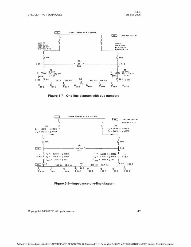
IEEECALCULATING TECHNIQUES Std 551-2006
Copyright © 2006 IEEE. All rights reserved. 49
Figure 3-7—One-line diagram with bus numbers
Figure 3-8—Impedance one-line diagram
Authorized licensed use limited to: UNIVERSIDADE DE SAO PAULO. Downloaded on September 14,2020 at 17:33:56 UTC from IEEE Xplore. Restrictions apply.

IEEEStd 551-2006 CHAPTER 3
50 Copyright © 2006 IEEE. All rights reserved.
3.5 Per-unit and ohmic manipulations2
Short-circuit calculations are made to solve the equation I = E/Z. Obtaining values of the
impedance Z is a time consuming effort when conducting a short-circuit analysis. The
impedance Z, given on the equipment nameplate or furnished by the equipment
manufacturer, may be identified either in per-unit or in ohmic values, but one or the other
must be used consistently in any calculation. The same study results will ultimately be
obtained for either ohmic or per-unit representation. Many engineers find the per-unit
system easier to use because impedance changes due to transformer ratios are
automatically taken into account. The per-unit system is a shorthand calculating technique
where all equipment and circuit impedances are converted to a common base.
In using the ohmic system, all impedances must be referred to the appropriate voltage
level by the square of the transformer turns ratio. With several levels of voltages, this can
become an added bookkeeping task. In the per-unit system, changing of impedance values
because of transformer ratios is unnecessary. For example, using the same voltage base as
the transformer primary and secondary voltages results in the transformer per-unit
impedance being the same on both sides of the transformer. Equipment manufacturers
usually state the impedance of electrical equipment in per-unit on the kVA and voltage
base of the equipment.
The per-unit impedances of machines (using the machine ratings as bases) of the same
type (induction motor, synchronous motor, synchronous generator, etc.) are approximately
the same for a broad range of machine sizes, while the ohmic values vary with the size of
the machine. Knowing that the per-unit impedances fall within a fairly narrow band is
advantageous when machine data must be estimated. Typical per-unit values are often
used in preliminary designs or for small motors where individual test reports are not
available.
In the per-unit system, there are many base quantities, including base apparent power
(kVA or MVA), base volts (volts or kV), base impedance (ohms), and base current
(amperes). Choosing any two automatically determines the other bases. The relationship
between base, per-unit, and actual quantities is as shown in Equation (3.8).
(3.8)
or rewritten
(3.9)
Normally, the base MVA is selected first and the most commonly used MVA bases are
10 MVA and 100 MVA, although any MVA or kVA base value may be used. Many
utilities express impedance as “percent” impedance on a 100 MVA base, where percent
impedance equals per-unit impedance times 100. The voltage at one level is chosen as the
2See Beeman [B1], Stevenson [B10], Weedy [B11].
per quantity unit actual quantitybase quantity
-----------------------------------------=
actual quantity per unit quantity( ) base quantity( )=
Authorized licensed use limited to: UNIVERSIDADE DE SAO PAULO. Downloaded on September 14,2020 at 17:33:56 UTC from IEEE Xplore. Restrictions apply.

IEEECALCULATING TECHNIQUES Std 551-2006
Copyright © 2006 IEEE. All rights reserved. 51
base voltage, which then determines the base voltage at the other levels using the primary
and secondary operating voltage rating of the transformers. Rated transformer primary and
secondary voltages are commonly used as the voltage bases.
For three-phase power systems, line-to-line voltage (usually expressed in kV) is used with
three-phase kVA or MVA base. The following equations apply to three-phase systems.
Equation (3.10) and Equation (3.11) convert the equipment and line data to a common
base when the base voltages match the equipment voltages.
Converting ohms to per-unit impedance:
(3.10)
Converting per-unit ohms from an equipment MVA base to a common MVA base where
base voltage = equipment voltage:
(3.11)
Converting per-unit ohms from an equipment voltage base to a common voltage base:
(3.12)
Combining Equation (3.11) and Equation (3.12):
(3.13)
Having determined the MVA and voltage bases, the current and impedance bases for each
voltage level can be determined. This provides a constant multiplier at each voltage level
to obtain the current or per-unit impedance by the use of Equation (3.9).
(3.14)
(3.15)
Similar expressions can be used for a single-phase system with care exercised to use only
quantities found in single-phase circuits. The current is the line current, the voltage is line-
to-neutral voltage, and the base is the single-phase kVA or MVA. For example:
ZpuZohmsMVAbase
kVLLBase2
-----------------------------------=
ZCommon baseZEquipment baseMVACommon base
MVAEquipment base---------------------------------------------------------------------------=
ZCommon base ZEquipment
kVLL Equipment
2
kVLL Common
2-------------------------------=
ZCommon base ZEquipmentMVACommon base( ) kVLL Equipment base
2( )
MVAEquipment base( ) kVLL Common base2( )
-----------------------------------------------------------------------------------------------=
IBase amps( )MVABase( )1000
3 kVLL---------------------------------------=
ZBase ohms( )kVLL
2( )1000
kVA-----------------------------
kVLL2
MVA-------------= =
Authorized licensed use limited to: UNIVERSIDADE DE SAO PAULO. Downloaded on September 14,2020 at 17:33:56 UTC from IEEE Xplore. Restrictions apply.

IEEEStd 551-2006 CHAPTER 3
52 Copyright © 2006 IEEE. All rights reserved.
(3.11a)
Per-unit ohms on equipment voltage base to common voltage base:
(3.12a)
(3.14a)
3.6 Network theorems and calculation techniques
The following network theorems and calculating techniques provide the basis for valid
methods of solving power system circuit problems.
3.6.1 Linearity
Linearity (see Griffith [B4] and Hoyt and Kennedy [B5]) is the most fundamental concept
to be discussed and is a powerful extension of Ohm’s Law. Examination of Figure 3-9 will
assist in understanding the basic principles. The simplified network is represented by the
single impedance element, R + jX. The circuit diagram shown is said to be linear for the
chosen excitation and response function. A plot of the response magnitude (current)
versus the source excitation magnitude (voltage) is a straight line for a linear element. This
is the situation shown for plot “A” (solid line) in the graph at the bottom of the figure.
When linearity exists, the plot applies to either the steady-state value of the excitation and
response functions or the instantaneous value of the functions at a specific time.
When linear dc circuits are involved, the current will double if the voltage is doubled. The
linear characteristic also holds for ac circuits provided the frequency of the driving voltage
is held constant. In a similar manner, it is possible to predict easily the response of a
constant impedance circuit (i.e., constant R, L, and C elements) to any magnitude of dc
source excitation or fixed frequency sinusoidal excitation based on the known response at
any other level of excitation. For the chosen excitation function of voltage and the chosen
response function of current, either dotted curve “B” or “C” would be examples of the
response characteristic of a non-linear element. Such nonlinear characteristics are often
encountered in the modeling of rotating machines and transformers, and the engineer must
be aware of the potential effects.
ZCommon baseZEquipment baseMVACommon base
MVAEquipment base---------------------------------------------------------------------------=
ZCommon base ZEquipmentkVLN equipment
2
kVLN common2
----------------------------------=
IBaseMVABase( )1000
kVLN---------------------------------------=
Authorized licensed use limited to: UNIVERSIDADE DE SAO PAULO. Downloaded on September 14,2020 at 17:33:56 UTC from IEEE Xplore. Restrictions apply.

IEEECALCULATING TECHNIQUES Std 551-2006
Copyright © 2006 IEEE. All rights reserved. 53
An important limitation of linearity is that the excitation source, if not independent, must
be linearly dependent on another (independent or dependent) source or network variable.
Ultimately in a linear circuit, all variables, including source, network, and load voltages
and currents are related to each other by a set of coefficients. This restraint, in effect,
forces a source to behave with a linear response.
3.6.2 Superposition
Superposition (see Griffith [B4] and Hoyt and Kennedy [B5]) is possible as a direct result
of linearity and hence is subject to the same restraints. The superposition theorem states
that if a network consists of linear elements and has several dc or fixed frequency ac
excitation sources (i.e., voltages), the total response (i.e., current) can be evaluated as the
sum of the currents caused by each voltage source acting separately with all other source
voltages reduced to zero or, similarly, all other current sources open circuited. Note that
this sum will be a simple algebraic sum in dc circuits and will be a vector sum in ac
circuits.
An example that illustrates this principle is shown in Figure 3-10. The written equation is
for the sum of the currents from each individual source of V = 10 V and V = 5 V. The
2 ohm and 6 ohm impedance values represent the sum of internal impedances of the
voltage sources and any other impedance in the source branches. The 5 ohm impedance
represents a load impedance.
Figure 3-9—Linearity
R L
i(t)
~ )(sin2 αω +tE
Authorized licensed use limited to: UNIVERSIDADE DE SAO PAULO. Downloaded on September 14,2020 at 17:33:56 UTC from IEEE Xplore. Restrictions apply.

IEEEStd 551-2006 CHAPTER 3
54 Copyright © 2006 IEEE. All rights reserved.
3.6.3 Thevenin equivalent circuit
This powerful circuit analysis tool is based on the fact that any active linear network,
however complex, can be represented by a single voltage source equal to the open-circuit
voltage across any two terminals of interest, in series with the equivalent impedance of the
network viewed from the same two terminals with all sources in the network inactivated
(i.e., voltage sources zero and current sources open). The validity of this representation
requires only that the network be linear. The existence of linearity is, therefore, a
necessary restraint. (Note that Thevenin equivalents can also be formed for multiphase
power systems.) The application of the Thevenin equivalent circuit can be appreciated by
again referring to the simple circuit of Figure 3-11 and developing the Thevenin
equivalent for the network with the switch in the open position as illustrated in the step-
by-step procedure. After connecting the 5-ohm load to the Thevenin equivalent network,
the solution is the same as in Figure 3-10, 0.9615 amperes. Using the simple Thevenin
equivalent shown for the entire left side of the network, it would be easy to examine the
response of the circuit as the value of the load impedance is varied. Caution, however, is
required to ensure that equipment models or buses of interest are not “absorbed” by the
process of forming a Thevenin equivalent. Once absorbed, relevant data pertaining to
individual contributions to total short-circuit current and bus voltages are unrecoverable
without completely resolving the entire circuit without using an equivalent.
Figure 3-10—Superposition
Authorized licensed use limited to: UNIVERSIDADE DE SAO PAULO. Downloaded on September 14,2020 at 17:33:56 UTC from IEEE Xplore. Restrictions apply.
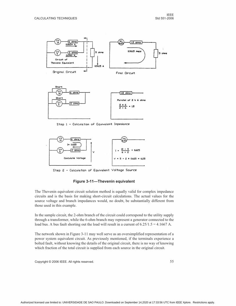
IEEECALCULATING TECHNIQUES Std 551-2006
Copyright © 2006 IEEE. All rights reserved. 55
The Thevenin equivalent circuit solution method is equally valid for complex impedance
circuits and is the basis for making short-circuit calculations. The actual values for the
source voltage and branch impedances would, no doubt, be substantially different from
those used in this example.
In the sample circuit, the 2-ohm branch of the circuit could correspond to the utility supply
through a transformer, while the 6-ohm branch may represent a generator connected to the
load bus. A bus fault shorting out the load will result in a current of 6.25/1.5 = 4.1667 A.
The network shown in Figure 3-11 may well serve as an oversimplified representation of a
power system equivalent circuit. As previously mentioned, if the terminals experience a
bolted fault, without knowing the details of the original circuit, there is no way of knowing
which fraction of the total circuit is supplied from each source in the original circuit.
Figure 3-11—Thevenin equivalent
Authorized licensed use limited to: UNIVERSIDADE DE SAO PAULO. Downloaded on September 14,2020 at 17:33:56 UTC from IEEE Xplore. Restrictions apply.

IEEEStd 551-2006 CHAPTER 3
56 Copyright © 2006 IEEE. All rights reserved.
3.6.4 Norton equivalent circuit
A Norton equivalent, Figure 3-12, that consists of a current source (triangle) in parallel
with an equivalent impedance can alternately be developed for the Thevenin equivalent
circuit. This representation is often used for computer solutions, but generally not for “by
hand” solutions in power system analysis work.
3.6.5 Millman's theorem
A direct result of Norton’s equivalent is Millman’s theorem (see Fich and Potter [B3]),
which states that when any number of voltage sources of arbitrary generated voltage and
finite internal impedance different from zero are connected in parallel, the resultant
voltage across the parallel combination is the ratio of the algebraic sum of the currents that
each source individually delivers when short circuited to the algebraic sum of the internal
admittances. Millman’s theorem can be used to simplify calculations in polyphase circuits
and has other applications.
3.6.6 Reciprocity
The general reciprocity (see Fich and Potter [B3]) theorem states that in networks
consisting of linear circuit elements, the ratio of excitation to response when only one
excitation is applied is constant when the positions of excitation and response are
interchanged. Specifically, this means that the ratio of the voltage applied in one branch to
the resulting current in a second branch of a network is the same as the ratio of the voltage
applied in the second branch to the resulting current in the first branch.
3.6.7 The sinusoidal forcing function3
It is a most fortunate truth that the excitation sources (i.e., driving voltage) for electrical
networks, in general, have a sinusoidal character and may be represented by a sine wave
plot of the type as previously illustrated in Figure 3-2 and Figure 3-3. There are two
important consequences of this circumstance. First, although the response (i.e., current)
for a complex R, L, C network represents the solution to at least one second-order
3See Griffith [B4].
Figure 3-12—Norton equivalent for a Thevenin equivalent circuit
Authorized licensed use limited to: UNIVERSIDADE DE SAO PAULO. Downloaded on September 14,2020 at 17:33:56 UTC from IEEE Xplore. Restrictions apply.

IEEECALCULATING TECHNIQUES Std 551-2006
Copyright © 2006 IEEE. All rights reserved. 57
differential equation, the steady-state result will be a sinusoid of the same frequency as the
excitation and differs only in magnitude and phase angle.
The second important item is that when the sinusoidal current is forced to flow in a
general impedance network of R, L, and C elements, the voltage drop across each element
will have a sinusoidal shape of the same frequency as the source. The sinusoidal character
of all the circuit responses makes the application of the Superposition technique to a
network with multiple sources surprisingly manageable. The necessary manipulation of
the sinusoidal terms is easily accomplished using the laws of vector algebra.
The only restraint associated with the use of the sinusoidal forcing function concept, is
that the circuit must be comprised of linear elements. While most circuits contain
nonlinearities, it is usually possible to restrict an analysis to a certain range of operating
conditions where linear characteristic hold.
3.6.8 Phasor representation
Phasor representation allows any sinusoidal forcing function to be represented as a phasor
in a complex coordinate system in the manner shown in Figure 3-13 (see Griffith [B4]).
The expression for the phasor representation of a sinusoid may assume any of the
following shorthand forms:
Exponential: Ee jφ
Rectangular: E (cosφ + jsinφ)
Polar: E/φ
These three forms are related as shown below.
Eejφ = E (cosφ + jsinφ) = E<φ
The network impedances can be represented as phasors using vectorial relationships and
the circuit current responses can be obtained through the simple vector algebraic
manipulation of the quantities involved. The need for solving complex differential
equations in order to determine the steady-state circuit response is completely eliminated.
The following restraints apply:
1) The sources must all be sinusoidal.
2) The frequency must remain constant.
3) The circuit R, L, and C elements must remain constant, i.e., linearity must exist.
Authorized licensed use limited to: UNIVERSIDADE DE SAO PAULO. Downloaded on September 14,2020 at 17:33:56 UTC from IEEE Xplore. Restrictions apply.

IEEEStd 551-2006 CHAPTER 3
58 Copyright © 2006 IEEE. All rights reserved.
3.6.9 Fourier representation4
This tool allows any non-sinusoidal periodic function to be represented as the sum of a dc
component and a series (infinitely long, if necessary) of ac sinusoidal functions.
Figure 3-14 shows a non-sinusoidal waveform without a dc component. The ac
components have frequencies that are an integral “harmonic” of the fundamental
frequency. The general mathematical form of the so-called “Fourier Series” is shown in
Equation (3.15).
(3.15)
where F0 is a dc term, F1 is a fundamental frequency (60 Hz in North American power
systems) term, and Fn are called “harmonics” of the fundamental and have frequency of
n2π f0. Each harmonic may have some nonzero phase angle θN.
4See Griffith [B4].
Figure 3-13—The phasor diagram
Mag. * cos φ
j Mag. * sin φ
Mag. (cos φ + j sin φ)
jX
(Inductive)
- jX
(Capacit ive)
-R R
Real Axis 0
Imaginary Axis
φ
f t( ) F0 2 Fn n2πf0 t θn+( )cos
n 1=
∞
+=
Authorized licensed use limited to: UNIVERSIDADE DE SAO PAULO. Downloaded on September 14,2020 at 17:33:56 UTC from IEEE Xplore. Restrictions apply.

IEEECALCULATING TECHNIQUES Std 551-2006
Copyright © 2006 IEEE. All rights reserved. 59
The importance of the Fourier representation is that the response to the original driving
function can be determined by first appropriately solving for each harmonic component
driving function and then summing all the individual solutions to find the total response
by superposition. Because each of the component response solutions is readily obtained,
the most difficult part of the problem becomes the modification of reactance and
capacitance of the network for each harmonic and the solution of the component driving
function. The individual harmonic voltages can be obtained in combination with
numerical integration approximating techniques through several well-established
mathematical procedures. The discussion of their use is better reserved for the many
excellent texts on the subject.
There are several rather abstract mathematical conditions that must be satisfied to permit
the use of a Fourier representation. The practical restraints are that the original driving
function must be periodic (repeating) and the network must remain linear for each of the
frequencies in the non-sinusoidal wave form.
3.6.10 Equivalence
The Equivalence Theorem (see Fich and Potter [B3]) states that at any given frequency,
any passive four-terminal network can be replaced by an equivalent star or delta network.
This fact is very useful in short-circuit calculations to reduce a system consisting of many
current loops and voltage nodes to a simple equivalent circuit. Figure 3-15 shows the
equations for both delta-star and star-delta transformations.
Figure 3-14—The Fourier representation
-1
0
1
0 0.5 1 1.5 2 2.5
Time in Cycles at 60 Hertz
f(t)
(p
.u.)
Authorized licensed use limited to: UNIVERSIDADE DE SAO PAULO. Downloaded on September 14,2020 at 17:33:56 UTC from IEEE Xplore. Restrictions apply.

IEEEStd 551-2006 CHAPTER 3
60 Copyright © 2006 IEEE. All rights reserved.
3.6.11 Parallel impedances
Where two or more impedances are paralleled and Zequiv. equals the equivalent
impedance, the relationships shown in Figure 3-16 are valid. In the case of two
impedances, the expression is reduced to the product of the two impedances divided by the
sum.
Figure 3-15—Delta-star impedance conversions
Authorized licensed use limited to: UNIVERSIDADE DE SAO PAULO. Downloaded on September 14,2020 at 17:33:56 UTC from IEEE Xplore. Restrictions apply.

IEEECALCULATING TECHNIQUES Std 551-2006
Copyright © 2006 IEEE. All rights reserved. 61
3.6.12 Analysis of unbalanced faults using symmetrical components5
An unbalanced fault condition is the most common circuit condition that invalidates the
single-phase (or positive sequence) equivalent circuit condition method for calculating
short-circuit current. The use of symmetrical components is the analytical technique most
commonly used under these circumstances. Unbalanced faults, such as line-to-ground
faults, line-to-line faults, and double line-to-ground faults require the use of symmetrical
components for the calculation of the short-circuit currents. Symmetrical components are
used to reduce an unbalanced system of phasors into three balanced systems of phasors
designated as positive, negative, and zero sequence components. Figure 3-17 is an
illustration of the system of symmetrical components. The subscripts A, B, and C
represent the three phases of voltage and the subscripts 1, 2, and 0 represent the positive,
negative, and zero sequence components.
5See Stevenson [B10], Westinghouse [B12], Rothe [B9].
Figure 3-16—Parallel impedances
Authorized licensed use limited to: UNIVERSIDADE DE SAO PAULO. Downloaded on September 14,2020 at 17:33:56 UTC from IEEE Xplore. Restrictions apply.

IEEEStd 551-2006 CHAPTER 3
62 Copyright © 2006 IEEE. All rights reserved.
Any three-phase set of unbalanced voltage phasors (or current phasors) can be resolved
into three balanced or symmetrical sets of phasors, i.e., positive sequence symmetrical
components, negative sequence symmetrical components, and zero sequence components,
as shown in Figure 3-18.
Figure 3-17—Symmetrical component balanced phasors
EA1
EB1
EC1
EA2
EC2
EB2
EA0
EB0
EC0
Positive Sequence Voltage Negative Sequence Voltage Zero Sequence Voltage
120€
120€
120€
120€
120€
120€
Authorized licensed use limited to: UNIVERSIDADE DE SAO PAULO. Downloaded on September 14,2020 at 17:33:56 UTC from IEEE Xplore. Restrictions apply.

IEEECALCULATING TECHNIQUES Std 551-2006
Copyright © 2006 IEEE. All rights reserved. 63
The use of symmetrical components in fault analysis is covered in more detail in
Chapter 11.
Symmetrical component techniques allow the user to solve for voltages and currents in
balanced sequence networks, and then convert the solution back to actual currents and
voltages. The relationship between the phase quantities in terms of their symmetrical
components is given below. Values of current can be substituted in place of the voltage in
the equation without any conversion factors. The equations are normally given as a set of
three to represent the individual phases [Equation (3.16)].
(3.16)
When using symmetrical components it is convenient to define an operator “a” such that:
a = 1∠120 = –0.5 + j0.866
Figure 3-18—Symmetrical components of unbalanced phasors
EA1
EB1
EC1
EA2
EC2
EB2
EA0
EB0
EC0
Positive Sequence Vo ltage Negative Sequence Voltage Zero Sequence Voltage
EA
EB
EC
Unbalanced set of three phase voltages
112€
115€
133€
120€
120€
120€
120€
120€
120€
Ea Ea0 Ea1 Ea2 Ea0 Ea1 Ea2
Eb Eb0 Eb1 Eb2 Ea0 Ea1 240 E+ a2∠ 120
Ec Ec0 Ec1 EC2 Ea0 Ea1 120 Ea2+ 240∠∠+=+ +=
∠+=+ +=
+ +=+ +=
Authorized licensed use limited to: UNIVERSIDADE DE SAO PAULO. Downloaded on September 14,2020 at 17:33:56 UTC from IEEE Xplore. Restrictions apply.

IEEEStd 551-2006 CHAPTER 3
64 Copyright © 2006 IEEE. All rights reserved.
a2 = 1∠240 = –0.5 – j0.866
Note that vector “a” is an operator with unit length and is oriented 120 degrees in counter-
clockwise rotation from reference axis. Figure 3-19 shows the property of a0, a1, and a2
and so on.
Using the operator “a” Equation (3.16) can now be rewritten as shown in Equation (3.17):
(3.17)
or in matrix form as in Equation (3.18):
(3.18)
with the matrix A defined as follows in Equation (3.19):
(3.19)
Ea Ea0 Ea1 Ea2
Eb Ea0 a2Ea1 aEa2
Ec Ea0 aEa1 a2Ea2+ +=
+ +=
+ +=
Figure 3-19—Operator “a” vectors
EA
EB
EC
1 1 1
1 a2 a
1 a a2
Ea0
Ea1
Ea2
=
A
1 1 1
1 a2 a
1 a a2
=
Authorized licensed use limited to: UNIVERSIDADE DE SAO PAULO. Downloaded on September 14,2020 at 17:33:56 UTC from IEEE Xplore. Restrictions apply.

IEEECALCULATING TECHNIQUES Std 551-2006
Copyright © 2006 IEEE. All rights reserved. 65
The inverse of the A matrix is as shown in Equation (3.20):
(3.20)
and
(3.21)
The equations above were written for the sequence voltages. A similar set of equations can
be written for the sequence current by interchanging the voltage symbol for a current
symbol. Note that if the zero sequence quantity, Ia0 (or Va0), equals zero then the vector
sum of IA + IB + IC (or VA + VB + VC) equals zero.
In the use of symmetrical components, the voltage is normally taken as line-to-neutral
voltage for the following reason. In an unbalanced set of EL-L voltage vectors, the sum of
voltages around the vector triangle is zero and the identity of zero sequence is not
apparent. Based on Equation (3.21), the zero sequence EL-L is zero, Ea0 = EAB + EBC +
ECA; however, Ea0 using EL-N voltage may not be zero. The vector diagram in Figure 3-20
illustrates the point.
In a grounded power system, the zero sequence impedance completes the circuit by
allowing the current to flow in the system neutral or in ground. The magnitude of current
in the return path is 3Ia0. Where 3Ia0 = In = Ia + I + Ic. When 3Ia0 = 0 = Ia + Ib + Ic, no
current flows in the neutral. Note that a three-phase three-wire (ungrounded) system will
require Ia0=0 because no neutral (or return) path exists for current flow.
A1– 1
3---
1 1 1
1 a a2
1 a2 a
=
Ea0
Ea1
Ea2
1
3---
1 1 1
1 a a2
1 a2 a
EA
EB
EC
A1–
EA
EB
EC
==
Figure 3-20—Zero sequence component of line-to-line and
line-to-neutral voltages
Authorized licensed use limited to: UNIVERSIDADE DE SAO PAULO. Downloaded on September 14,2020 at 17:33:56 UTC from IEEE Xplore. Restrictions apply.

IEEEStd 551-2006 CHAPTER 3
66 Copyright © 2006 IEEE. All rights reserved.
It is interesting to note that the delta winding of a delta-wye or wye-delta connected
transformer or delta connected loads provide no current path to neutral and no zero
sequence currents will exist in delta connected systems. However, it can be shown that
zero sequence circulating currents can exist in the delta winding of a transformer but not
pass through the transformer.
3.6.13 Sequence impedances
The impedance of elements in a symmetrical electrical system may be resolved into
positive, negative, and zero sequence components. In a balanced three-phase system, only
positive sequence impedances are required and only positive sequence voltage drops and
current flows result from the analysis. (Recall the equivalence of the positive sequence
and the “a” phase under balanced three-phase conditions.) In systems where the phase
impedances are not equal or where unbalanced faults are simulated using symmetrical
networks, positive, negative, and perhaps zero sequence voltage drops and current flows
will result.
The relationships between sequence voltages and currents follow Ohms’ law as shown in
Equation (3.22) and Figure 3-21 below.
(3.22)
In general, the impedances of static elements are the same in positive and negative
sequences, but may differ in the zero sequence. For rotating machines, the impedances are
usually different for all sequences.
Rothe [B9], Stevenson [B10], and Westinghouse [B12] provide positive, negative, and
zero sequence impedance representations of the various system components for network
calculations.
E1 I1Z1
E2 I2Z2
E0 I0Z0=
=
=
Figure 3-21—Sequence network diagrams for Equation (3.22)
Authorized licensed use limited to: UNIVERSIDADE DE SAO PAULO. Downloaded on September 14,2020 at 17:33:56 UTC from IEEE Xplore. Restrictions apply.

IEEECALCULATING TECHNIQUES Std 551-2006
Copyright © 2006 IEEE. All rights reserved. 67
Figure 3-22 illustrates how sequence components are obtained for a transformer. The
same source connection is used for other equipment. Positive sequence impedances are
determined by the use of a balanced three-phase source while zero sequence impedances
are determined by connecting all three-phase leads to a common single-phase source.
3.7 Extending a three-phase short-circuit calculation procedures
program to calculate short-circuit currents for single-phase branches
The following describes the extension of a three-phase short-circuit calculation techniques
program to include fault current calculations for single-phase branch circuits supplied
line-to-line by a three-phase system. The procedure for the special system limitation given
below prevents the need to use symmetrical components.
The procedure assumes that the three-phase system is not appreciably unbalanced by the
single-phase branches, further that there are no single-phase rotating machines
contributing to the short-circuit duty, and that positive and negative sequence impedances
are equal. The latter assumption suggests that procedure is applied with reasonable
accuracy only to first-cycle short-circuit calculations when the contribution from three-
phase rotating machines is important because machine positive sequence impedances
become greater than negative as time passes.
Figure 3-22—Test set-up used to obtain the sequence components of a
transformer
Authorized licensed use limited to: UNIVERSIDADE DE SAO PAULO. Downloaded on September 14,2020 at 17:33:56 UTC from IEEE Xplore. Restrictions apply.

IEEEStd 551-2006 CHAPTER 3
68 Copyright © 2006 IEEE. All rights reserved.
The procedure has two steps. First, special handling of the single-phase circuit input data
is necessary and second, applicable results must be multiplied by √3/2 (= 0.866). This
procedure is an expansion oriented toward computer use of a general procedure described
in the Industrial Power Systems Handbook [B1]. The input data handling is developed for
the single-phase branch circuit as shown in Figure 3-23. To obtain these results by
computer, all single-phase circuit input impedance data is converted to per-unit on the
study three-phase base and a single-phase base voltage equal to the study three-phase line-
to-line base voltage. Input data is handled as noted below.
Conversion of single-phase circuit data to per-unit on a three-phase study base requires the
following:
1) For a two-conductor feeder use the impedance of one conductor (one phase to
neutral, NOT the round loop impedance).
2) For a single-phase transformer, per unitize the data based on the single-phase kVA
base and 0.5 times the nameplate impedance. The transformer X/R ratio used is
approximately equivalent to the X/R ratio of a three-phase transformer of 3 times
the single-phase kVA.
3) For a single-phase reactor “element,” enter one half the actual resistance and
reactance expressed in ohms or in per-unit.
4) The equivalent three-phase calculation results are multiplied by √3/2 (= 0.866) to
obtain the single-phase short-circuit duties. The program bus voltage could also be
entered as 1/0.866 = 1.155 times the line-to-line voltage to obtain the results
directly in amperes.
Authorized licensed use limited to: UNIVERSIDADE DE SAO PAULO. Downloaded on September 14,2020 at 17:33:56 UTC from IEEE Xplore. Restrictions apply.

IEEECALCULATING TECHNIQUES Std 551-2006
Copyright © 2006 IEEE. All rights reserved. 69
3.8 Representing transformers with non-base voltages
Occasionally, a power system includes transformers that have voltage ratios that differ
from the power system nominal values of base voltage chosen. This difference can have
an influence on the calculated fault current levels. The concern is the handling of the
transformer impedances and correction due to differences in rated and base voltages.
Usually a correction of transformer percent impedance due to a different operating tap
other than transformer rated or flat taps is not done unless test data provides this
information. Depending upon the design of the tap section of the transformer, the percent
impedance of the transformer on other taps is unknown without the transformer tap test
data. If there is a change, it is usually not linear or known to vary with any known
expression with tap position. Rather than guessing the new value of transformer
impedance on other taps, it may be considered a constant.
Several system conditions are possible that will effect the manner in which the
transformer per-unit impedance and base voltages are represented in the network. It is
Figure 3-23—Single-phase branch circuit connected line-to-line to a three-
phase system. Diagrams show location of single-phase short-circuit at F0.
A
B
C
Source Im pedance or
Remainder of
three-phase network
13.8 kV
1-3/C-4/0
300 Ft
500 kVA
1 Phase
13.8/0.24 kV
Z = 4%
F0
Schematic Diagram
13.8 kV
13.8 kV
Source
Equiv.
350 MVA
X/R = 7.10
1-3/C-4/0
300 Ft
500 kVA
1 Phase
13.8/0.24 kV
Z = 4%
F0
One-Line Diagram
13.8 kV
13.8 kV
0.004 + j0.0284
F0
Impedan ce Diagram
10 MVA Base
Zs
0.001 + j0.0005 Zc
0.0784 + j 0.3922
240 V
Authorized licensed use limited to: UNIVERSIDADE DE SAO PAULO. Downloaded on September 14,2020 at 17:33:56 UTC from IEEE Xplore. Restrictions apply.

IEEEStd 551-2006 CHAPTER 3
70 Copyright © 2006 IEEE. All rights reserved.
easy for the power system engineer to become frustrated, confused, and not make the
necessary corrections. Diagrams in Figure 3-24 and the explanation below should provide
some guidance on this subject. On the diagrams, differences from the rated tap,
transformer voltage rating, and base voltage of those used in Figure 3-1a are noted with
a#. For the condition when the transformer voltages equal the base voltages, nothing needs
to be corrected. This includes transformers that are operating off rated taps as shown in
Figure 3-1a and Figure 3-24c. In all other cases, there could be an impedance or voltage
base change depending on how the calculations are done.
In addition, samples are given where the bus operating voltage is different than the base
voltage. Most short-circuit calculations assume the prefault bus voltage is equal to the
base voltage when an initial load flow calculation is not made or the procedure in IEEE
Std C37.010™ [B8] is followed. In the following examples, the prefault bus voltage is a
concern only for that bus. If the primary voltage is high, as shown in Figure 3-24g, there is
no change in the 4.16 kV bus fault level. However, a fault on the transformer primary
would be affected by the higher 13.8 kV voltage.
Several conditions exist that will affect the degree in which data changes will have to be
made to transformers that have voltages or voltage ratios different than the base voltages.
These include manual calculations or the use of computer programs that treat all
transformers as if they were on rated taps. An example is the condition shown in
Figure 3-24e where the transformer rated taps and base voltages are equal, but the
transformer tap is not equal to the primary base voltage. For the manual calculation, a base
voltage and impedance change are required. Also, there will be many cases where no
transformer impedance change or base voltage change will be required; these are
automatically handled within the computer program.
Transformer taps can be on either side of the transformer. The need to change the
transformer impedance will depend on which side of the transformer the system base
voltage is to be held equal to the transformer voltage. In the samples shown, the 13.8 kV
(primary side) base voltage was fixed. The sample calculations in the figures use a
constant X/R ratio of the source and the transformer to keep calculations simple. In cases
where the transformer impedance should be modified before being placed in the network,
the expression given in Equation (3.12) (repeated here for convenience) is used. Such a
condition occurs when the transformer rated tap voltages do not match base voltages.
(3.12)
A special case occurs when one of the transformer rated tap voltages matches the base
voltages and the second transformer tap does not. In this case, the easiest procedure is to
change the base voltage of the side that does not match so that it does. This is easily done
on radial systems and will require other base voltages of equipment to be changed so that
all impedances are on the same base. In examples Figure 3-24e and Figure 3-24h, all
impedances on the 4.16 kV side of the transformer will have to be placed on a 4.2667 kV
base. Other transformers connected to the 4.16 kV system will have 4.2667 kV as one of
the base voltages.
ZCommon base ZEquipment
kVLL Equipment
2
kVLL Common
2-------------------------------=
Authorized licensed use limited to: UNIVERSIDADE DE SAO PAULO. Downloaded on September 14,2020 at 17:33:56 UTC from IEEE Xplore. Restrictions apply.

IEEECALCULATING TECHNIQUES Std 551-2006
Copyright © 2006 IEEE. All rights reserved. 71
For looped systems, it may not be possible to change the base voltage because different
transformers could cause a common bus to have a conflicting base voltage. In this case,
the procedure is to choose a base voltage, forcing the non-conforming equipment to fit.
Figure 3-24k shows a means of transformer representation to force the base voltage, a
method used in many computer programs. If the program does not have the facility to
model taps, the transformer could be entered as three branches provided that the program
uses a driving voltage and a “ground” or fault bus. The “ground” bus is not the same as the
source bus used or “internal voltage” bus used in some programs.
The common configuration is not the best for illustrating the procedure because the fault
shorts out one shunt connection of the transformer. A 4.16 kV impedance between the
transformer and fault would produce a voltage rise at the secondary of the transformer and
some current would flow in that branch.
The transformer tap value is often in per-unit of the transformer rated taps with the
expression below.
(3.23)
When the transformer voltage ratio does not equal the base voltage ratio and a program
with taps representation is used then a fictitious tap value can be used to resolve the
difference. The expression is:
(3.24)
The nameplate transformer impedance requires modification if the untapped winding
voltage rating does not equal the base voltage.
In the examination of the sample configurations, it appears that the fault duty on the
secondary side is not fixed for a given transformer. For a given transformer, it was noted
above that the impedance was taken to be constant over the tap range. Given that
statement, the fault duty in MVA on the secondary side should be constant. Comparing
Figure 3-1a and Figure 3-24c shows such conditions where the fault current is different.
This is best illustrated by comparing the volt-ampere to the fault. Both Figure 3-1a and
Figure 3-24c provide the same value.
From Figure 3-1a: MVA = 17.35 × 4.16 × = 125 MVA
From Figure 3-24h: MVA = 16.91 × 4.2667 × = 125 MVA
For breakers applied to 4.16 kV systems, the breakers have a constant volt-ampere
capability between its minimum and maximum voltage rating. Therefore, the numbers
above are being applied at the same percent of maximum breaker capability.
Tap value Tapped winding rated voltageRated tap voltage
--------------------------------------------------------------------------=
Fictitious tap value Tapped winding rated tap voltage( ) Untapped winding base voltage( )Untapped winding rated voltage( ) Tapped winding base voltage( )
---------------------------------------------------------------------------------------------------------------------------------------------------------------------------------------=
3
3
Authorized licensed use limited to: UNIVERSIDADE DE SAO PAULO. Downloaded on September 14,2020 at 17:33:56 UTC from IEEE Xplore. Restrictions apply.

IEEEStd 551-2006 CHAPTER 3
72 Copyright © 2006 IEEE. All rights reserved.
Figure 3-24f and Figure 3-24g have a condition where the transformer tap or high primary
voltage would make the secondary prefault voltage high if no load was placed on the
transformer. In these cases, it was assumed that the voltage was the result of a power flow
calculation and the prefault current flow through the transformer resulted in the bus
voltage being one per-unit. Using the no load prefault voltage would result in the fault
currents being higher by the ratio of (no load voltage/prefault voltage). Figure 3-24f would
equal 17.57 kA and Figure 3-24g would equal 17.85 kA.
In Figure 3-24 the term
is defined as Base kV Ratio = Base kV at transformer primary / Base kV at transformer
secondary and Transformer kV ratio = Transformer primary tap kV / Transformer
secondary tap kV.
Base kV ratio
Transf. kV ratio------------------------------------------
Figure 3-1a—Transformer kV equals base kV
Transformer rated kV ratio equals base kV ratio
Authorized licensed use limited to: UNIVERSIDADE DE SAO PAULO. Downloaded on September 14,2020 at 17:33:56 UTC from IEEE Xplore. Restrictions apply.

IEEECALCULATING TECHNIQUES Std 551-2006
Copyright © 2006 IEEE. All rights reserved. 73
Figure 3-24b—Transformer rated kV not equal to base kV
Transformer rated kV ratio equals base kV ratio
Figure 3-24c—Transformer tapped kV equals to base kV
Transformer rated kV ratio not equal to base kV ratio
Authorized licensed use limited to: UNIVERSIDADE DE SAO PAULO. Downloaded on September 14,2020 at 17:33:56 UTC from IEEE Xplore. Restrictions apply.

IEEEStd 551-2006 CHAPTER 3
74 Copyright © 2006 IEEE. All rights reserved.
Figure 3-24d—Transformer rated and tapped kV ratio equals base kV ratio
Secondary prefault kV not equal to bus base kV
Figure 3-24e—Transformer rated kV equals to base kV
Transformer tapped kV not equal to base kV
Secondary prefault kV not equal to bus base kV
Authorized licensed use limited to: UNIVERSIDADE DE SAO PAULO. Downloaded on September 14,2020 at 17:33:56 UTC from IEEE Xplore. Restrictions apply.

IEEECALCULATING TECHNIQUES Std 551-2006
Copyright © 2006 IEEE. All rights reserved. 75
Figure 3-24f—Transformer rated kV equals to base kV
Transformer tapped kV not equal to base kV
Secondary prefault kV equal to bus base kV
Figure 3-24g—Transformer kV equals base kV
Transformer kV equals base kV ratio
Primary prefault kV not equal to bus base kV
Authorized licensed use limited to: UNIVERSIDADE DE SAO PAULO. Downloaded on September 14,2020 at 17:33:56 UTC from IEEE Xplore. Restrictions apply.

IEEEStd 551-2006 CHAPTER 3
76 Copyright © 2006 IEEE. All rights reserved.
Figure 3-24h—Transformer kV not equal to base kV
Transformer kV ratio equals base kV ratio
Figure 3-24i—Transformer tap kV not equal to base kV
Transformer rated kV ratio equals base kV ratio
Secondary prefault voltage not equal to base kV
Authorized licensed use limited to: UNIVERSIDADE DE SAO PAULO. Downloaded on September 14,2020 at 17:33:56 UTC from IEEE Xplore. Restrictions apply.

IEEECALCULATING TECHNIQUES Std 551-2006
Copyright © 2006 IEEE. All rights reserved. 77
Figure 3-24j—Transformer tap kV not equal to base kV
Transformer kV ratio equals base kV ratio
Secondary prefault voltage not equal to base kV
Authorized licensed use limited to: UNIVERSIDADE DE SAO PAULO. Downloaded on September 14,2020 at 17:33:56 UTC from IEEE Xplore. Restrictions apply.

IEEEStd 551-2006 CHAPTER 3
78 Copyright © 2006 IEEE. All rights reserved.
3.9 Specific time period and variations on fault calculations
Short-circuit calculations used in industrial and commercial power systems have several
purposes. One purpose is to establish the maximum calculated available short-circuit
duties to be compared with the equipment short-circuit ratings or capabilities. Bolted
three-phase short-circuits are normally assumed. First-cycle maximum symmetrical duties
are used to compare equipment with first-cycle equipment ratings (momentary or close-
and-latch) when rated on a symmetrical current basis, while total (asymmetrical) duties
are required for equipment rated on a total current basis. In either case, the X/R ratio of the
Figure 3-24k—Transformer tap kV not equal to base kV
Transformer kV ratio not equal to base kV ratio
Authorized licensed use limited to: UNIVERSIDADE DE SAO PAULO. Downloaded on September 14,2020 at 17:33:56 UTC from IEEE Xplore. Restrictions apply.

IEEECALCULATING TECHNIQUES Std 551-2006
Copyright © 2006 IEEE. All rights reserved. 79
fault is also required to calculate the asymmetry of the short-circuit current to ensure that
the maximum possible current (ac plus dc) does not exceed equipment ratings. The
application of equipment is explained in more detail in Chapter 11. Short-circuit current
magnitudes evaluated at times ranging from 1.5 to 4 cycles at 60 Hz are used to determine
the interrupting duties for ac medium- and high-voltage circuit breaker applications.
The second purpose is to establish currents useful for protective relaying. Both minimum
and maximum currents at the point of fault and as distributed through the system are of
interest. Three-phase, line-to-ground, and other types of fault studies may be required.
First-cycle maximum short-circuit currents may be used when providing settings for
instantaneous or high-speed relays. The currents at longer times after short-circuit
initiation are needed for relay settings and also for estimating the performance of time
delay relays. Currents calculated at “approximately 30 cycles” are recommended to be
used for back-up time delay relays. Often the current values after 30 cycles following the
fault initiation are desired for both maximum and minimum generating or operating
conditions.
The first-cycle short-circuit currents are also used in determining the magnetic forces that
the equipment will be subjected to until the short circuit is cleared. As previously
mentioned, these forces are a function of the instantaneous values of current squared.
The maximum value is the crest value of the maximum asymmetric current that the circuit
can produce. It is available in the first half cycle after the short circuit occurs. Equipment
nameplate data does not provide the magnetic force data directly. Instead, the maximum
magnetic forces are indirectly given by the maximum current the equipment can carry.
The total duration of the short circuit determines the thermal energy available to be
released in the equipment.
This energy is a function of the amplitude of the current and the time duration.
The thermal energy Joules (3.25)
where R is the equipment resistance.
It can be shown that the energy content is a function of the system X/R ratio because the
total current (ac plus dc) must be accounted for in the evaluation of the thermal energy
produced. Again, equipment nameplate data does not provide the thermal energy and
magnetic force data directly, but is encompassed by the equipment maximum current
carrying capacity and the time for which this current is allowed to flow.
The equivalent impedance to be used for calculating fault currents at different time
periods is shown in the following table. The reactance values are general and may differ
between standards. The applicable ANSI-approved standards specify the impedance
multipliers that should be applied to the rotating machine impedances in the equivalent
circuit. These values are given in IEEE Std C37.010 [B8].
Te R i2 td �=
Authorized licensed use limited to: UNIVERSIDADE DE SAO PAULO. Downloaded on September 14,2020 at 17:33:56 UTC from IEEE Xplore. Restrictions apply.

IEEEStd 551-2006 CHAPTER 3
80 Copyright © 2006 IEEE. All rights reserved.
In Table 3-1, depending on the purpose of the calculation, X"d (modified) may be used
with a multiplier in some cases and in other cases X'd is being used.
When the maximum value of short-circuit current 30 cycles after fault initiation is desired,
the equivalent circuit (used like a Thevenin equivalent) should include positive sequence
impedances yielding toward maximum current magnitudes. In addition, the circuit should
include any rotating machines that might still be contributing to the short-circuit fault.
This equivalent circuit usually contains generators represented by transient impedance and
minimum utility system impedances representing maximum available short-circuit
currents.
Induction motors close to the fault will normally either have been disconnected by their
undervoltage devices, or the magnetic energy stored in the motor will be completely
decayed and hence will not contribute short-circuit currents at 30 cycles.
Depending on the type of excitation system on synchronous generators or motors, 30 cycle
short-circuit current decay associated with synchronous machines still connected to the
system will vary greatly. Machine excitation systems that rectify the ac bus voltage for
field current may decay to near zero during a nearby fault, while other excitation system
capable of current forcing could provide 1.5 to 3 times full-load current at 30 cycles. For
maximum short-circuit current some engineers include these motors using transient
impedances in the equivalent circuit.
Fault durations of 30 cycles or more that are in close proximity to rotating synchronous
machines will most likely cause the synchronous machine to pull out of step with the
remainder of the system. In such cases, a dynamic model of the system would be required
for more accurate results.
It should be noted that the maximum line-to-line or line-to-ground short-circuit current
can become greater than the maximum three-phase short-circuit current for a persistent
fault because the positive sequence impedance of the equipment is increasing while the
negative and zero sequence impedances remain constant. Also, the zero sequence
Table 3-1—Appropriate reactance values for the different cycles
Equipment1st cyclecurrents
3–5 cyclecurrents
30 cyclecurrents
Remote sources X X X
Generators X"d X"d(modified) X'd*
Synch. motors X"d X"d(modified) X'd or
X'd(modified)*
Induction motors X" X"(modified) ×
Authorized licensed use limited to: UNIVERSIDADE DE SAO PAULO. Downloaded on September 14,2020 at 17:33:56 UTC from IEEE Xplore. Restrictions apply.

IEEECALCULATING TECHNIQUES Std 551-2006
Copyright © 2006 IEEE. All rights reserved. 81
impedance may be smaller than the positive and negative sequence impedance at the time
of fault initiation.
When the minimum value of a 30 cycle bolted three-phase short-circuit current is required
in checking relay operation, the equivalent circuit should simulate operating conditions
that tend to minimize short-circuit currents, and should include the minimum number of
generators connected and the maximum utility source impedance value representing the
minimum available short-circuit currents. Generators are generally represented by
transient impedances. Induction and synchronous motor contributions are omitted.
3.10 Determination of X/R ratios for ANSI fault calculations
The breaker duty fault point X/R ratio is found from separate X only and R only networks
derived from the equivalent circuit as described in 5.3.2 of IEEE Std C37.010 [B8]. There
is no completely accurate means of combining two or more parallel circuits with different
values of X/R into a single circuit with one value of X/R. The current from individual
branches of the parallel circuits and sources behind them will be the sum of several
exponentially decaying terms, usually with different decay rates, while the X/R ratio
calculated from a single Thevenin equivalent circuit contains just one such term.
For radially-fed circuits, there will be no difference between solving for the fault point
X/R ratio using either the Xonly and Ronly approach or the (single) Thevenin equivalent
approach. (Note that “radially-fed” means that there is only one source of fault current.)
However, even the addition of a single motor at the end of a radial feeder with a
significantly different machine X/R ratio as compared to the system impedance will cause
a different X/R ratio at the fault point between the two calculation methods. It should be
noted that an accurate method of determining the fault point X/R ratio would be to solve
the system differential equations with the system represented with resistors, inductors, and
capacitors. Even small systems would become difficult to solve. However, the method of
using separately derived networks results in a calculated X/R ratio that is generally more
conservative (larger) than the (single) Thevenin equivalent method. The Thevenin
equivalent method cannot ensure a conservative X/R ratio and should not be used for
asymmetry current multipliers for breaker duties. However, the use of a Thevenin
equivalent should be adequate for relay application.
It should be noted that the resistance network for first-cycle and for interrupting time
calculations is varied for machines by the same multipliers as used for the internal
reactance. This caution is noted because some X values may have been increased by
reactance multiplying factors, and if the corresponding R values are not similarly
increased, the X/R ratio and thus the asymmetrical current multiplying factor will be
unrealistically high.
3.11 Three-winding transformers
When a three-winding transformer forms part of the system under analysis,
Figure 3-24b shows the equivalent circuit and the impedance expressions that are
applicable. Note that the equations that make up Equation (3.26) are not the same as the
Authorized licensed use limited to: UNIVERSIDADE DE SAO PAULO. Downloaded on September 14,2020 at 17:33:56 UTC from IEEE Xplore. Restrictions apply.

IEEEStd 551-2006 CHAPTER 3
82 Copyright © 2006 IEEE. All rights reserved.
equations used for delta-star impedance conversions. Furthermore, Equation (3.26)
applies only when all impedances are expressed on a common MVA base. This reflects
the method used when the impedance tests are preformed on the transformer. Once having
made a T equivalent, the delta-star conversion can be used for delta impedance
representation if desired.
The transformer impedance values are normally stated in percent and generally on the
highest kVA winding base. The transformer nameplate will state which base is used for
the impedances. Often when solving the conversion equations, one leg of the equivalent
circuit will contain a negative impedance. The negative impedance must be retained to
obtain the correct solution. However, it can be added to a series positive impedance if a
computer program does not allow a negative impedance. Node “D” is an artificial point in
the equivalent circuit and has no meaning in system evaluations.
(3.26)
3.12 Duplex reactor
A duplex reactor is a single reactor center tapped, or two reactors physically arranged, so
that their magnetic fields are interlinked. With current flowing in one winding only, the
reactor behaves the same as a single stand-alone reactor. Simultaneous currents flowing in
each winding creates a different situation. The coupling factor, fc, defines the linking of
magnetic fields between the two windings. The flow of current in one winding will induce
a voltage in the other winding, (transformer action), which will in turn affect the other
winding current flow. A positive coupling factor effectively increases the impedance
between nodes “A” and “B,” while a negative coupling factor reduces the impedance. A
reactor used to reduce fault current magnitudes will have a positive coupling factor.
Table 3-2 provides representative coupling factors.
Xa 1 2⁄ XHX XHT XXT–+( )Xb 1 2⁄ XXT XHX XHT–+( )Xc 1 2⁄ XHT XXT XHX–+( )=
=
=
Figure 3-1—Equivalent circuit of a three-winding transformer
Authorized licensed use limited to: UNIVERSIDADE DE SAO PAULO. Downloaded on September 14,2020 at 17:33:56 UTC from IEEE Xplore. Restrictions apply.
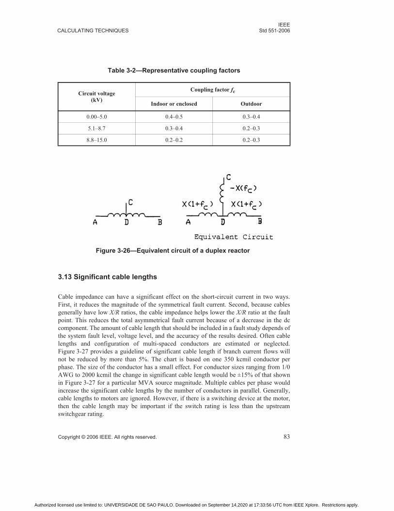
IEEECALCULATING TECHNIQUES Std 551-2006
Copyright © 2006 IEEE. All rights reserved. 83
3.13 Significant cable lengths
Cable impedance can have a significant effect on the short-circuit current in two ways.
First, it reduces the magnitude of the symmetrical fault current. Second, because cables
generally have low X/R ratios, the cable impedance helps lower the X/R ratio at the fault
point. This reduces the total asymmetrical fault current because of a decrease in the dc
component. The amount of cable length that should be included in a fault study depends of
the system fault level, voltage level, and the accuracy of the results desired. Often cable
lengths and configuration of multi-spaced conductors are estimated or neglected.
Figure 3-27 provides a guideline of significant cable length if branch current flows will
not be reduced by more than 5%. The chart is based on one 350 kcmil conductor per
phase. The size of the conductor has a small effect. For conductor sizes ranging from 1/0
AWG to 2000 kcmil the change in significant cable length would be ±15% of that shown
in Figure 3-27 for a particular MVA source magnitude. Multiple cables per phase would
increase the significant cable lengths by the number of conductors in parallel. Generally,
cable lengths to motors are ignored. However, if there is a switching device at the motor,
then the cable length may be important if the switch rating is less than the upstream
switchgear rating.
Table 3-2—Representative coupling factors
Circuit voltage(kV)
Coupling factor fc
Indoor or enclosed Outdoor
0.00–5.0 0.4–0.5 0.3–0.4
5.1–8.7 0.3–0.4 0.2–0.3
8.8–15.0 0.2–0.2 0.2–0.3
Figure 3-26—Equivalent circuit of a duplex reactor
Authorized licensed use limited to: UNIVERSIDADE DE SAO PAULO. Downloaded on September 14,2020 at 17:33:56 UTC from IEEE Xplore. Restrictions apply.

IEEEStd 551-2006 CHAPTER 3
84 Copyright © 2006 IEEE. All rights reserved.
3.14 Equivalent circuits
It is sometimes desirable to make an equivalent circuit of a larger remotely connected
system to reduce unnecessary detail in a portion of a system. These systems could have
one or more connections to the system under study. A single tie equivalent can be easily
determined by the fault current flow from the remote system and its phase angle. A system
with two or more non-independent connections requires more effort. Figure 3-28 shows
the steps involved for a three point “T” representation. A “pi” representation could also be
used. The procedure is to make an equivalent network and determine an equivalent
impedance value. For a two point equivalent, this requires solving for three unknowns by
placing three separate faults on the system. The equivalent impedance determined from
the equations could have two possible solutions. One answer may involve a negative
impedance. While a negative impedance is a mathematically correct solution, it is not
generally the answer used. The second solution has a positive impedance and is generally
the impedance used.
A three point equivalent requires solving six unknowns. The number of equations to be
solved varies by the expression (points2 + points)/2 and quickly becomes too cumbersome
to do by hand. Some computer network analysis programs can perform this function. An
alternate method is to work with the network to be reduced and to combine impedances by
using series, parallel, and delta-star conversions until the desired nodes remain.
Figure 3-27—Approximate cable lengths for a 5% change in fault current
Authorized licensed use limited to: UNIVERSIDADE DE SAO PAULO. Downloaded on September 14,2020 at 17:33:56 UTC from IEEE Xplore. Restrictions apply.

IEEECALCULATING TECHNIQUES Std 551-2006
Copyright © 2006 IEEE. All rights reserved. 85
3.15 Zero sequence line representation
When unbalanced fault calculations are required involving cables or transmission lines
that are mutually coupled in the zero sequence network, special handling of the circuits is
required. Many computer based programs can handle these types of circuits in any line
combination. Coupled lines between the same two buses are easily handled by changing
the zero sequence impedance when one or two lines are in service. Lines that connect
between different buses require a 1:1 ratio mutual-coupling transformer. The condition of
the lines being common on one bus is a condition that can be handled by hand or in
computer programs without zero sequence mutual coupling. It requires that the two line
sections be handled as shown in Figure 3-29 and is similar to the duplex reactor previously
shown in Figure 3-26.
Figure 3-28—“T” equivalent circuit
Authorized licensed use limited to: UNIVERSIDADE DE SAO PAULO. Downloaded on September 14,2020 at 17:33:56 UTC from IEEE Xplore. Restrictions apply.

IEEEStd 551-2006 CHAPTER 3
86 Copyright © 2006 IEEE. All rights reserved.
3.16 Equipment data required for short-circuit calculations
One of the most time consuming and critical items required in a short-circuit analysis is
obtaining available data. The less data that is assumed, the better and more accurate the
results. There are conditions when most of the data may initially have to be estimated,
such as when designing a new system. As the system becomes finalized, specific
equipment data may be available and the results are more pertinent. On existing systems,
the amount of estimated data is greatly reduced.
An up-to-date one-line diagram is needed. If one is not available, site inspection is
required to determine switchgear and load center connection points. There may be cases
where no information exists regarding the interconnection of plant loads back to the utility
supply. The lack of information is usually the result of a temporary “quick fix” that never
properly became documented and over time became permanent. A time consuming tracing
of conductors is required to identify its connection to known point. One great value of the
short-circuit study is therefore an up-to-date one-line diagram.
In the discussion in 3.16.1, the available data used for short-circuit calculations that can be
obtained from equipment nameplates is noted by an *. Other data required will have to be
itemized and requested or gathered separately. The data is then converted to ohms or per-
unit ohms before it can be used in the analysis.
3.16.1 Utility sources
The equipment impedance data for the utility source must be obtained from the utility
company. When requesting the data, specify at what point the source contribution
equivalent is to be desired, form desired (per-unit, MVA, or amperes), base voltage used
for the calculation, X/R ratio at the point specified, and if data desired is for three-phase or
three-phase and line-to-ground calculations. A one-line diagram sketch is often helpful in
defining the point of the equivalent. Most utilities do not include the industrial user as a
source of short-circuit current unless in-plant generation is present. In addition, the
equivalent source impedance will be from a complex R + jX calculation. Generally, the
source impedance from neither a separate R and X (Ronly and Xonly) nor first-cycle and
Figure 3-29—Equivalent zero sequence mutual circuit
Authorized licensed use limited to: UNIVERSIDADE DE SAO PAULO. Downloaded on September 14,2020 at 17:33:56 UTC from IEEE Xplore. Restrictions apply.
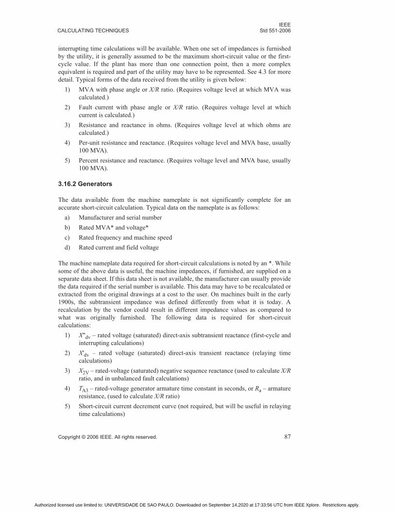
IEEECALCULATING TECHNIQUES Std 551-2006
Copyright © 2006 IEEE. All rights reserved. 87
interrupting time calculations will be available. When one set of impedances is furnished
by the utility, it is generally assumed to be the maximum short-circuit value or the first-
cycle value. If the plant has more than one connection point, then a more complex
equivalent is required and part of the utility may have to be represented. See 4.3 for more
detail. Typical forms of the data received from the utility is given below:
1) MVA with phase angle or X/R ratio. (Requires voltage level at which MVA was
calculated.)
2) Fault current with phase angle or X/R ratio. (Requires voltage level at which
current is calculated.)
3) Resistance and reactance in ohms. (Requires voltage level at which ohms are
calculated.)
4) Per-unit resistance and reactance. (Requires voltage level and MVA base, usually
100 MVA).
5) Percent resistance and reactance. (Requires voltage level and MVA base, usually
100 MVA).
3.16.2 Generators
The data available from the machine nameplate is not significantly complete for an
accurate short-circuit calculation. Typical data on the nameplate is as follows:
a) Manufacturer and serial number
b) Rated MVA* and voltage*
c) Rated frequency and machine speed
d) Rated current and field voltage
The machine nameplate data required for short-circuit calculations is noted by an *. While
some of the above data is useful, the machine impedances, if furnished, are supplied on a
separate data sheet. If this data sheet is not available, the manufacturer can usually provide
the data required if the serial number is available. This data may have to be recalculated or
extracted from the original drawings at a cost to the user. On machines built in the early
1900s, the subtransient impedance was defined differently from what it is today. A
recalculation by the vendor could result in different impedance values as compared to
what was originally furnished. The following data is required for short-circuit
calculations:
1) X"dv – rated voltage (saturated) direct-axis subtransient reactance (first-cycle and
interrupting calculations)
2) X'dv – rated voltage (saturated) direct-axis transient reactance (relaying time
calculations)
3) X2V – rated-voltage (saturated) negative sequence reactance (used to calculate X/Rratio, and in unbalanced fault calculations)
4) TA3 – rated-voltage generator armature time constant in seconds, or Ra – armature
resistance, (used to calculate X/R ratio)
5) Short-circuit current decrement curve (not required, but will be useful in relaying
time calculations)
Authorized licensed use limited to: UNIVERSIDADE DE SAO PAULO. Downloaded on September 14,2020 at 17:33:56 UTC from IEEE Xplore. Restrictions apply.

IEEEStd 551-2006 CHAPTER 3
88 Copyright © 2006 IEEE. All rights reserved.
6) X0 – zero sequence reactance (used in unbalanced fault calculations for grounded
generators)
One item not supplied as part of the generator nameplate or data sheet that may be
required for relaying time calculations is the type of voltage regulator used with the
generator. See 3.9 for the effects of regulators on extended time fault calculations.
3.16.3 Synchronous motors
The data required for synchronous motors is the same as that furnished for generators.
Machine nameplate data may not be sufficiently complete for an accurate short-circuit
analysis. Typical data on the nameplate is as follows:
a) Manufacturer and serial number
b) Rated MVA* and voltage*
c) Rated frequency and machine speed
d) Rated current and field voltage
The machine nameplate data required for short-circuit calculations is noted by an *. While
some of the above data is useful, the machine impedances, if available, are given on a
separate data sheet. If a data sheet is not available, the manufacturer can usually provide
the data required if the serial number is available. This data may have to be recalculated or
extracted from the original drawings at a cost to the user. Some manufacturers may only
furnish one transient or subtransient impedance for motors, which is usually the rated
voltage X"dv value that is desired for short-circuit calculations. The following data is
required for short-circuit calculations:
1) X"dv – rated voltage (saturated) direct-axis subtransient reactance (first-cycle and
interrupting calculations)
2) X'dv – rated voltage (saturated) direct-axis transient reactance (relaying time
calculations)
3) X2V – rated-voltage (saturated) negative sequence reactance (used to calculate X/Rratio and unbalanced faults)
4) TA3 – rated-voltage generator armature time constant in seconds, or Ra – armature
resistance, (used to calculate X/R ratio)
5) Short-circuit current decrement curve (not required, but may be useful in relaying
time calculations)
6) X0 – zero sequence reactance (used in unbalanced fault calculations for grounded
motors. Most wye connected motors are not connected to system neutrals)
One item not supplied as part of the motor nameplate or data sheet that may be required
for relaying time calculations is the type of voltage regulator used with the motor. Most of
the present day regulators are of the potential source type and do not supply sustained
short-circuit currents. See 3.9 for the effects of regulators on extended time fault
calculations.
Authorized licensed use limited to: UNIVERSIDADE DE SAO PAULO. Downloaded on September 14,2020 at 17:33:56 UTC from IEEE Xplore. Restrictions apply.

IEEECALCULATING TECHNIQUES Std 551-2006
Copyright © 2006 IEEE. All rights reserved. 89
3.16.4 Induction motors
Some data required for short-circuit studies that include induction motors is on the motor
nameplate. But the nameplate data is not sufficiently complete for an accurate short-circuit
calculations. Typical data on the nameplate is as follows:
a) Manufacturer and serial number
b) Rated HP or MVA* and voltage*
c) Rated frequency and motor speed*
d) Rated current and NEMA code letter*
Data required for short-circuit calculations is noted by an *. Machine impedances are
seldom furnished on a separate data sheet. However, if a data sheet is available, the
manufacturer usually specifies the locked-rotor current that can be used to estimate the
motor subtransient impedance. More detailed impedance data is available at a cost, but is
usually not justified. Different impedance data is furnished for the motor at both stall and
running conditions and the resistances furnished may not include the one required for
short-circuit calculations. The motor starting reactance is most often used for short-circuit
calculation. However, the resistance to be used for short-circuit calculations is lower than
the starting resistance provided on the data sheet. Unless a short-circuit resistance is
provided, typical motor X/R ratio curves can be used.
Data for smaller motors is usually estimated because the cost of obtaining this information
is not justified.
3.16.5 Transformers
Transformer nameplates usually provide most of the data required for short-circuit
calculations. Typical data on the nameplate is as follows:
1) Manufacturer and serial number
2) Rated MVA* and frequency
3) Rated primary and secondary voltages*
4) Rated current and taps available*
5) Transformer percent impedance*
6) Number of windings, winding connection and phase relationship* (needed for
unbalanced fault calculations)
7) Manufacturer test report.
The nameplate data required for short-circuit calculations is noted by an *. Note that the
transformer nameplate data is given as a percent impedance and not percent reactance and
is generally given on the self cooled rating unless otherwise specified. The reactance is
determined once the percent resistance is known. The transformer X/R ratio is not on the
nameplate, but can be determined from the transformer test sheet or losses, if provided.
Some data sheets do provide the% resistance as a piece of data; otherwise, the% resistance
is determined by:
Authorized licensed use limited to: UNIVERSIDADE DE SAO PAULO. Downloaded on September 14,2020 at 17:33:56 UTC from IEEE Xplore. Restrictions apply.

IEEEStd 551-2006 CHAPTER 3
90 Copyright © 2006 IEEE. All rights reserved.
or
The standard phase relationship of a delta-wye or wye-delta transformer is that the high-
voltage side leads the low-voltage side by 30 degrees for positive phase sequence systems.
When performing unbalanced fault calculations, the positive sequence current and voltage
shifts by either +30 degrees or –30 degrees, while the negative sequence current and
voltage have the same phase shift but in the opposite direction. Note that one side of the
transformer is selected as reference. With the reference established, the phase shift is
applied following the general rule of “HV side leads LV side for positive sequence, and
HV lags LV for negative sequence.” As an example, suppose that a delta-wye transformer
has the HV winding selected as reference. Based on this choice of reference, the positive
sequence LV side values will lag the positive sequence HV side values, and the negative
sequence LV side values will lead the negative sequence HV side values. The signs on the
phase shifts would be exactly reversed if the LV side were selected as reference and the
HV side values were required to be shifted with respect to the LV side values. There will
be no shift of the zero sequence current since there is no path for this current component to
flow. The zero sequence voltage is determined by the zero sequence impedance times the
zero sequence current flow on each side of the transformer.
3.16.6 Reactors
The reactor nameplate usually provides most of the data required for short-circuit
calculations. Typical data on the nameplate is:
1) Manufacturer and serial number
2) Rated voltage* and frequency
3) Rated current* and taps available*
4) Reactor percent impedance*
5) Reactor ohms* (not always provided)
6) Percent voltage drop* (not always provided)
7) Manufacturer test report
The nameplate data required for short-circuit calculations is noted by an *. The reactor X/R ratio is not on the nameplate, but can be determined from the reactor test sheet or losses,
if provided. Some data sheets do provide the reactance, the resistance, and reactor “Q”
factor as a piece of data. Not all the above * items can be used directly for a short-circuit
calculation. For example, the percent impedance is on the “through” kVA (volts × amps)
of the reactor and for a three-phase reactor the through kVA is:
%R Total watt loss no load loss–( )100
Transformer rating in volt amperes----------------------------------------------------------------------------------------=
%R Full load winding loss( )100
Transformer rating in volt amperes----------------------------------------------------------------------------------------=
Through kVA 31RatedVRated, LL=
Authorized licensed use limited to: UNIVERSIDADE DE SAO PAULO. Downloaded on September 14,2020 at 17:33:56 UTC from IEEE Xplore. Restrictions apply.

IEEECALCULATING TECHNIQUES Std 551-2006
Copyright © 2006 IEEE. All rights reserved. 91
The impedance can also be determined from the voltage drop as follows:
Impedance in ohms = volt drop in volts / IRated
The base for the percent voltage drop (when used) is line-to-line rated voltage.
For a three-phase reactor, the “self” kVA is as follows:
3.16.7 Capacitors
The inclusion of capacitor data is usually not necessary under most conditions. See the
chapter on capacitor contributions to short-circuit currents to determine the actual extent
to which capacitors will affect the first-cycle calculations. If inclusion of the capacitor
date is required, the capacitors nameplate is complete for short-circuit calculations. The
data on the nameplate will be as follows:
1) Manufacturer and serial number
2) Rated voltage* and frequency
3) Rated kvar*
The nameplate data required for short-circuit calculations is noted by an *. The capacitor
X/R ratio is not on the nameplate, but is generally very high and can be determined from
the capacitor loss test sheet, if it is provided. If assuming the X/R ratio, a value from 200 to
300 should be acceptable, because the series cable resistance quickly overwhelms the
capacitor resistance. The length of cable to the capacitor bank is important and should be
included.
3.16.8 Static regenerative drives
The inclusion of static regenerative drive data will be necessary in the first-cycle
calculations. (Note that non-regenerative drives are not sources of fault current and need
not be considered.) The rectifier transformer and drive motor size is required. Typical data
on the drive transformer nameplate is as follows:
1) Manufacturer and serial number
2) Rated voltage* and frequency
3) Rated primary and secondary voltages*
4) Rated current and taps available*
5) Transformer percent impedance*
6) Number of windings, winding connection and phase relationship
The nameplate data required for short-circuit calculations is noted by an *. The drive
transformer X/R ratio is not on the nameplate, but can be determined from the transformer
test sheet or losses, if provided. Some data sheets do provide the percent resistance as a
piece of data; otherwise, the percent resistance is determined by:
Self kVA 31Rated
2 X=
Authorized licensed use limited to: UNIVERSIDADE DE SAO PAULO. Downloaded on September 14,2020 at 17:33:56 UTC from IEEE Xplore. Restrictions apply.
IEEEStd 551-2006 CHAPTER 3
92 Copyright © 2006 IEEE. All rights reserved.
or
Note that the drive transformer nameplate data is given as a percent impedance and not
percent reactance. The reactance is determined once the percent resistance is known.
The size of the driven motor load is also required to determine the short-circuit current
contribution or equivalent source impedance. The motor size may have to be extracted
from drawings. The motor data needed is the same as given for motors in 3.16.3 and
3.16.4. For short-circuit calculations where the drive is modeled as an induction motor, the
equivalent drive impedance should be greater than the typical impedance of an induction
motor with the same rating.
3.16.9 Breakers, contactors, and current transformers
The inclusion of breaker, contactor, or current transformer impedances is seldom done in
short-circuit calculations. These impedances are more significant in low-voltage system
analysis than for the higher-voltage systems. The impedances of series connected trip or
thermal overload devices in the power circuit on low-voltage systems can greatly reduce
the available fault current downstream from such devices and therefore should be included
when required. For fractional horsepower motor loads, the thermal overload devices will
have an impedance magnitude in ohms as compared to cable impedances in milliohms.
3.16.10 Cables
The connecting cables will not have any impedance data stamped on them. Data typically
found on the cable includes the following:
a) Manufacturer
b) Rated voltage*
c) Type of cable* and insulation type*
d) Size of conductor*
In addition, the following data is required:
1) Length
2) Type of cable construction (1/C or 3/C)
3) Number of cables in parallel and physical spacing
4) Type of cable duct used (steel, fiber, cable tray, direct burial, etc.)
Data shown on cable and required for short-circuit calculations is noted by an *. The
impedance data per unit of length must be determined from other sources such as
%R Total watt loss no load loss–( )100
Transformer rating in volt amperes----------------------------------------------------------------------------------------=
%R Full load winding loss( )100
Transformer rating in volt amperes----------------------------------------------------------------------------------------=
Authorized licensed use limited to: UNIVERSIDADE DE SAO PAULO. Downloaded on September 14,2020 at 17:33:56 UTC from IEEE Xplore. Restrictions apply.

IEEECALCULATING TECHNIQUES Std 551-2006
Copyright © 2006 IEEE. All rights reserved. 93
manufacturer’s literature or general cable impedances in texts. The cable manufactures
literature is preferred, because insulation thickness may differ between manufacturers
where as most references provide typical impedance values (see IEEE Std 141-1993 [B6],
IEEE Std 242-2001 [B7], Beeman [B1], Stevenson [B10]). References usually provide
positive sequence impedance, which is used in three-phase faults. For unbalanced faults,
the zero sequence cable data is required and not usually provided in references.
The zero sequence impedances of cables differ from that of the positive and negative
sequence and is dependent upon the physical configuration and the impedances of the
ground return paths. Formulas for calculating cable impedances are available in many
books such as Elements of Power System Analysis [B10].
3.16.11 Transmission lines
The impedance data for connecting transmission lines should be based on the line
configuration. Drawings or sketches showing wire size, type of conductor material, and
conductor spacing are required. In addition, circuit length, type and size of ground wire,
and earth resistance must be obtained.
The impedance data per unit of line length will have to determined from other sources
such as Elements of Power System Analysis [B10] or the Transmission and DistributionReference Book [B13].
Authorized licensed use limited to: UNIVERSIDADE DE SAO PAULO. Downloaded on September 14,2020 at 17:33:56 UTC from IEEE Xplore. Restrictions apply.

IEEEStd 551-2006 CHAPTER 3
94 Copyright © 2006 IEEE. All rights reserved.
3.17 Bibliography
[B1] Beeman, Donald, Industrial Power Systems Handbook.
[B2] Close, C. M., The Analysis of Linear Circuits.
[B3] Fich, S., and J. L. Potter, Theory of A.C. Circuits, Chapter 6, p.214–228.
[B4] Griffith, M. Shan, “A Penetrating Gaze at One Open Phase,” IEEE Transactions onIndustry Applications, Nov/Dec, 1977 p. 504.
[B5] Hoyt, W. H., Jr., and J. E. Kennedy, Engineering Circuit Analysis.
[B6] IEEE Std 141™-1993, IEEE Recommended Practice for Electric Power Distribution
for Industrial Plants (IEEE Red Book), Chapter 4, page 115.6, 7
[B7] IEEE Std 242™-2001, IEEE Recommended Practice for Protection and Coordination
of Industrial and Commercial Power Systems (IEEE Buff Book), Chapter 2.
[B8] IEEE Std C37.010-1999 (Reaff 2005), IEEE Guide for AC High-Voltage Circuit
Breakers Rated on a Symmetrical Current Basis.
[B9] Rothe, F.S., An Introduction to Power System Analysis, Chapter 3, 6, and 7.
[B10] Stevenson, W.D. Jr., Elements of Power System Analysis. McGraw Hill.
[B11] Weedy, B.M., Electric Power Systems.
[B12] Westinghouse, Applied Protective Relaying, Chapter 2.
[B13] Westinghouse, Transmission and Distribution Reference Book.
6IEEE publications are available from the Institute of Electrical and Electronics Engineers, 445 Hoes Lane, P.O.Box 1331, Piscataway, NJ 08855-1331, USA (http://standards.ieee.org/).7The IEEE standards or products referred to in this subclause are trademarks of the Institute of Electrical andElectronics Engineers, Inc.
Authorized licensed use limited to: UNIVERSIDADE DE SAO PAULO. Downloaded on September 14,2020 at 17:33:56 UTC from IEEE Xplore. Restrictions apply.

Copyright © 2006 IEEE. All rights reserved. 95
Chapter 4 Calculating short-circuit currents for systems without ac delay
4.1 Introduction
This chapter describes the calculation of three-phase short-circuit currents for systems
without ac decay [i.e., No AC Decay (NACD)]. The procedures described here are
appropriate for equipment sizing evaluations when generation is not located in the
immediate electrical area where the calculations for equipment applications are being
performed. (Note that procedures in other chapters are appropriate for calculations when
generation is present in the local electrical area.) IEEE Std C37.010™-1999 [B3]1
identifies power system generation, regardless if it is utility or local (plant) generation, as
either “local” or “remote” to the fault location. A generator is considered electrically
remote if the ratio of the network reactance from the generator terminals to the faults point
is ≥1.5Xd". Alternatively a remote generator may be defined as being more than one
transformation away from the fault point. Remote generation will not exhibit ac decay
characteristics. From the correlation between “remote” and “no ac decay,” it can be
implied that a system “with no ac decay” does not have any fault current contribution from
nearby rotating equipment. This could be applicable to some subtransmission systems
serving residential loads or an industrial plant on a weekend where all the rotating
equipment is disconnected. Without any ac decay current, the first cycle and interrupting
time calculations use the same impedance network and therefore the symmetrical currents
are the same.
This chapter is limited to the consideration of short-circuit currents that occur under the
following conditions:
1) Short-circuit fault currents that occur in low-voltage ac systems and medium-
voltage ac systems operating at a constant frequency and electrically remote from
any generators.
2) For the duration of the short circuit, there is no change in the source driving
voltage or voltages that caused the initial short-circuit current to flow. In addition,
system impedances remain constant.
3) The fault impedance is zero and has no current limiting effect.
4) Motor fault current contribution is negligible.
5) For simplification, only three-phase faults will be considered. Unbalanced faults
are covered in Chapter 11.
4.2 Purpose
The object of this chapter is to give recommended standardized procedures for the
calculation of short-circuit current in systems with NACD. The application and selection
1The numbers in brackets correspond to those of the bibliography in 4.8.
Authorized licensed use limited to: UNIVERSIDADE DE SAO PAULO. Downloaded on September 14,2020 at 17:33:56 UTC from IEEE Xplore. Restrictions apply.

IEEEStd 551-2006 CHAPTER 4
96 Copyright © 2006 IEEE. All rights reserved.
of interrupting equipment based on the calculated fault currents are covered in Chapter 10.
No ac decay calculations are the simplest of the fault calculations and will serve as the
basis for the more complex fault current calculations. Fault currents with ac decay are
covered in Chapter 5 and Chapter 6. A sample one-line diagram will be used to show the
method of calculation and will increase in detail as motors and generators are added in the
later chapters. Hand calculations will be made at several locations and computer-
generated results will be given for selected other buses. The one-line diagram used is
similar to the diagram in the IEEE Std 399™-1997 (IEEE Brown Book) [B2].
4.3 ANSI guidelines
The calculation procedure to be used will be based on IEEE Std C37.010 [B3]. An
understanding of the analytical techniques of the ANSI method should help in interpreting
other calculating procedures such as IEC 909:1977 [B1].
IEEE Std C37.010 [B3] includes three other system conditions, as given in Chapter 3
(3.2), to be used when calculating fault currents. These are as follows:
1) The pre-fault bus voltage is 1.0 p.u.
2) Separate resistance and reactance networks are to be used to determine the fault
point X/R ratio. This Xsep/Rsep ratio is to be used to calculate the total
asymmetrical fault current. As an alternative, Z/Rsep can be considered the same as
Xsep/Rsep.
3) Load currents are much smaller than the fault current and are therefore neglected.
In IEEE Std C37.010 [B3], several simplified methods are listed for use where the current
determined by an E/X calculation (instead of E/Z) meets specific fault current or X/R ratio
criteria. For example, when the fault current is less than 80% of the breaker duty, an E/Xcalculation can be used. To determine if the current calculated by the simplified methods
meets these criteria, most of the effort that is needed for the detailed ANSI calculation is
already done. Because having several methods to calculate breaker duty current could lead
to confusion, the detailed ANSI calculation will be used here. Most computer programs
that follow the ANSI recommended method use the more detailed ANSI procedure.
In this chapter, the symmetrical ac component of the short-circuit current has a constant
rms magnitude for the duration of the fault. Thus, the rms magnitude of the ac component
of current for the system considered is independent of time and will have a constant value
determined by the system’s highest pre-fault voltage and equivalent series impedance. In
Chapter 2, asymmetry was discussed and was shown to depend on the fault point X/R ratio
and on the point on the voltage wave at which the fault is initiated. A fault current flowing
from a remote source may be asymmetrical and have both an ac and a dc component. The
dc component is a transient and decays with time, while the ac component is a constant-
amplitude sinusoid. In Chapter 2, several different theoretical and empirical equations
were given that relate the maximum peak and rms currents in the first cycle to the ac
symmetrical current. For the sample calculations in this chapter, the “Violet Book”
equations will be used and are repeated below.
Authorized licensed use limited to: UNIVERSIDADE DE SAO PAULO. Downloaded on September 14,2020 at 17:33:56 UTC from IEEE Xplore. Restrictions apply.

CALCULATING SHORT-CIRCUIT CURRENTS FOR SYSTEMS IEEEWITHOUT AC DECAY Std 551-2006
Copyright © 2006 IEEE. All rights reserved. 97
The first cycle Violet Book equations are as follows in Equation (4.1) and Equation (4.2):
(4.1)
(4.2)
where τ = 0.49 –
Equation (4.2) can be rewritten to calculate the total rms current at other points in time as
shown in Equation (4.3).
(4.3)
where τ is in cycles at 60 Hz.
Equation (4.1) and Equation (4.2) can be used to calculate the maximum asymmetry
during the first cycle, while Equation (4.3) can be used for times greater than 1 cycle.
Peak currents are often associated with equipment rated less than 1000 V; rms currents are
used with higher-voltage equipment. See the tables in Chapter 2 for the comparisons of the
approximation equation peaks with the actual peaks. When equipment operating times are
given in cycles at a particular frequency, the time can be ratioed to 60 Hz. For example,
five cycles at 50 Hz is the same time as six cycles at 60 Hz.
The dc current decrement for a simple single circuit of one branch is an exponential decay.
In a multi-branch power system, a single X/R ratio is only an approximation. Each branch
will actually have its own time constant and the total current will decay at some rate that is
dependent on the combined effect. There is no single time constant that will exactly
describe the dc decrement of a multi-branch total fault current.
For the purpose of simplicity and conservatism, ANSI has recommended that the
following simplified procedure be used to determine the X/R ratio for a particular fault.
The system impedance diagram is converted to a separate resistance (R) diagram and a
separate reactance (X) diagram. The resistance and reactance diagrams are then reduced to
a simple resistance (R) and a reactance (X) value at the fault point. These values are then
used to determine the system X/R at the fault point. The X/R value in turn determines the
system dc time constant and consequently the rate of decay of the transient dc fault
current.
Ipeak Iac peak 1 e
2πτX R⁄( )
----------------–
+� �� �� �
21ac rms 1 e
2πτX R⁄( )
----------------–
+� �� �� �
= =
Irms Iac rms2 Idc
2+ Iac rms 1 2e
4πτX R⁄( )
----------------–
+= =
0.1e
X R⁄( )3
----------------
Irms Iac rms 1 2e
4πτX R⁄( )
----------------–
+=
Authorized licensed use limited to: UNIVERSIDADE DE SAO PAULO. Downloaded on September 14,2020 at 17:33:56 UTC from IEEE Xplore. Restrictions apply.

IEEEStd 551-2006 CHAPTER 4
98 Copyright © 2006 IEEE. All rights reserved.
4.4 Fault calculations
ANSI fault calculations can be done in per-unit or in ohms with transformer ratios taken
into account. The samples used in this book will be shown using the per-unit method. The
steps in calculating ANSI fault currents are as follows:
1) Obtain an up-to-date one-line diagram.
2) Determine the impedance of each branch and source for the time period of
concern.
3) Reduce the network impedances to single Rsep and Xsep values using separate Rand X network reductions.
4) Calculate the fault current by combining the separate R and X values from step 3)
into a complex impedance at the fault point or by using the optional complex
impedance network impedance determined in step 4).
5) Calculate the fault point X/R ratio using Xsep/Rsep [step 3)] or, alternatively, Z/Rsep
[step 4)].
6) Calculate any asymmetrical currents using results of step 5) and step 6).
7) Calculate the branch contributions, if required.
8) Optional: Reduce the network impedances to a single Rsep value using a separate
R network reduction. Reduce the network impedances to a single complex
impedance using complex network reductions.
4.5 Sample calculations
4.5.1 Sample calculation #1
The complete sample one-line diagram that will be used is given elsewhere in this book. It
includes motors and generators that will be included in calculations in the following
chapters. In this chapter the utility is the only short-circuit source. A reduced one-line
diagram is shown in Figure 4-1.
For a fault on 2.4 kV bus 36:T13 SEC, the total impedance to the fault is the addition of
the series impedances to the fault point. This is a special case because the total impedance
is not affected by any parallel feeder ties between MILL-1 and MILL-2 buses. Closing
either the 480 V breaker on cable C-T12-1 or the 13.8 kV switch on cable C-J5 would
require the paralleling of transformers T-1 and T-2 with some cable impedances. This
would reduce the effective impedance between the utility and MILL-2 bus and increase
the fault level at bus 36:T13 SEC. The equipment raw data and per-unit data are given in
Table 4-1. The manual calculations and a typical computer printout are provided on the
pages that follow.
Table 4-1—Per-unit impedances of branches
Branch Per-unit R Per-unit X
UTIL 0.00045 0.00999
T-line 0.00139 0.00296
Authorized licensed use limited to: UNIVERSIDADE DE SAO PAULO. Downloaded on September 14,2020 at 17:33:56 UTC from IEEE Xplore. Restrictions apply.

CALCULATING SHORT-CIRCUIT CURRENTS FOR SYSTEMS IEEEWITHOUT AC DECAY Std 551-2006
Copyright © 2006 IEEE. All rights reserved. 99
Transf T-2 0.00313 0.05324
Cable C-M1 0.00118 0.00098
Cable C-M2 0.00079 0.00065
Transf T-13 0.02289 0.22886
Sum 0.02983 0.29668
Table 4-1—Per-unit impedances of branches (continued)
Branch Per-unit R Per-unit X
Figure 4-1—Equivalents and impedance one-line diagram for
sample calculations
Authorized licensed use limited to: UNIVERSIDADE DE SAO PAULO. Downloaded on September 14,2020 at 17:33:56 UTC from IEEE Xplore. Restrictions apply.

IEEEStd 551-2006 CHAPTER 4
100 Copyright © 2006 IEEE. All rights reserved.
The per-unit (p.u.) current with 1.00 p.u. source voltage is as follows:
The fault current is as follows:
The fault point X/R ratio is as follows:
For a fault on bus 36:T13 SEC with the 13.8 kV bus tie open, the fault point X/R ratio by
separate R and X and complex impedance reduction is the same as the value shown above
because there were not any parallel circuits.
The maximum asymmetrical rms current in the first cycle is, from Equation (2.3),
A sample computer printout for bus 36:T13 SEC is shown below.
* BUS: 36:T13 SEC ***** 8.068 KA AT -84.26 DEG ( 33.54 MVA): X/R = 9.95 KV = 2.400 Ze = 0.0298306 +j 0.2966802 (Complex) SYM kA*1.6 = 12.91 ASYM kA Based on X/R ratio = 11.64 kA
CONTRIBUTIONS TO FAULT: BUS to BUS MAG ANG 31:FDR P 36:T13 SE 8.068 -84.26
As an option, the symmetrical fault current could have been calculated using only the
reactance (0.29668). The fault symmetrical current would be 8.109 kA for a slightly more
conservative answer.
4.5.2 Sample calculation #2
Closing the 13.8 kV bus tie would increase the fault level and would also result in a
parallel circuit, which results in the fault point X/R ratio by separate R and X and the
IpuEZ---
1.0
0.02983 j0.29668+-----------------------------------------------
1.0
0.29818------------------- 3.354 pu at 84.258°–= = = =
IIpu MVAbase×
3 kV----------------------------------
3.354 10×100 3 2.4××------------------------------------ 8.0685 kA at 84.258°–= = =
XR---
0.29668
0.02983------------------- 9.9457= =
τ 0.49 0.1e
X R⁄( )3
----------------
– 0.4864= =
Irms Iac rms 1 2e
4πτX R⁄( )
----------------–
+� �� �� �
8.0685 1.4228( ) 11.642 kA= = =
Authorized licensed use limited to: UNIVERSIDADE DE SAO PAULO. Downloaded on September 14,2020 at 17:33:56 UTC from IEEE Xplore. Restrictions apply.

CALCULATING SHORT-CIRCUIT CURRENTS FOR SYSTEMS IEEEWITHOUT AC DECAY Std 551-2006
Copyright © 2006 IEEE. All rights reserved. 101
complex impedance reduction being different. First, paralleling the two transmission lines
and main transformers results in the impedances shown in Table 4-2.
Separate R and X paralleling of the transmission lines and transformers gives R =
0.002136 and X = 0.028075. The complex paralleling of the same two branches would
result in 0.002142 + j 0.028075, which has a slightly higher resistance. Table 4-3 shows
the impedance results for the separate R and X values all the way to the fault point.
Using the complex math paralleling, the sum would be 0.027452 + j0.268025 instead of
0.027446 and j0.26803 as shown by separate R and X reductions.
The per-unit fault current using separate R and X would be as follows:
Table 4-2—Parallel equivalent of T-lines and transformers
T-line and transf T1 T-line and transf T2
P.U. R P.U. X P.U. R P.U. X
0.00139 0.00296 0.00139 0.00296
0.00266 0.05324 0.00313 0.05324
Sum 0.00405 0.05620 0.00452 0.05620
Table 4-3—Separate R and X equivalents of T-lines and transformers
Branch P.U. R P.U. X
UTIL 0.00045 0.00999
T-Line and transf T1 in parallel withT-line and transf T2
(from above) 0.002136 0.02808
Cable C-M1 0.00118 0.00098
Cable C-M2 0.00079 0.00065
Transf T-13 0.02289 0.22886
Sum (separate R and X) 0.027446 0.26856
IpuEZ---
1.0
0.027446 j0.26856+--------------------------------------------------
1.0
0.27996------------------- 3.7043 pu at 84.165°–= = = =
Authorized licensed use limited to: UNIVERSIDADE DE SAO PAULO. Downloaded on September 14,2020 at 17:33:56 UTC from IEEE Xplore. Restrictions apply.

IEEEStd 551-2006 CHAPTER 4
102 Copyright © 2006 IEEE. All rights reserved.
The fault current is:
As an option, to calculate the fault current, the complex impedance to the fault point can
be used. The fault current using the complex network reduction to four decimal places is
8.9111 kA at –84.165º. The fault point X/R ratio is calculated from the separate R and Xnetwork reductions to be 9.7655. For this example, the current magnitude and its angle by
either network reduction are nearly the same. However, there can be cases where the
current and X/R ratio difference is greater. This occurs when parallel branches that have
wide differences in X/R ratios are present in the system.
4.5.3 Sample calculation #3
In this example, transformer T13 is changed and has a rating of 2.5 MVA, 13.2/2.3 kV,
5.75% impedance, and the selected operating tap is 13.53 kV. Because the transformer
voltage rating does not match the 13.8 kV base voltage, two items should be changed, one
is the transformer impedance and the other is a base voltage. To correct the impedance to
the primary 13.8 kV voltage base, Equation (3.12) from Chapter 3 is used.
The original 5.75% Z or the modified 5.261% Z can be entered into some computer
programs with the 13.53 kV tap and the transformer impedance will be corrected for tap
position. However, for hand calculations or computer programs without transformer tap
capabilities, a second step is required to correct for the transformer tap position. The same
equation as shown above can be used to calculate the change in transformer percent
impedance in one step. Two steps are shown for clarity.
Using an X/R ratio of 10, the transformer T13 per-unit impedance on the 10 MVA
(13.53 kV) system base is as follows:
0.02200 + j0.21999
IIpu MVAbase×
3kV----------------------------------
3.7043 10×1000 3 2.4××--------------------------------------- 8.9111 kA at 84.165°–= = =
XR---
0.26856
0.027446---------------------- 9.785= =
ZCommon base ZEquipment
kVEquipment base
2
kVCommon base
2----------------------------------=
ZCommon base 5.75( )13.22
13.82
------------ 5.261%==
ZCommon base 5.261( )13.532
13.22
--------------- 5.5273%==
Authorized licensed use limited to: UNIVERSIDADE DE SAO PAULO. Downloaded on September 14,2020 at 17:33:56 UTC from IEEE Xplore. Restrictions apply.

CALCULATING SHORT-CIRCUIT CURRENTS FOR SYSTEMS IEEEWITHOUT AC DECAY Std 551-2006
Copyright © 2006 IEEE. All rights reserved. 103
The secondary system base voltage is 2.3 × 13.53/13.2 = 2.3575 kV.
Table 4.4 shows the branch impedance values for this example.
The per-unit current with 1.00 p.u. source voltage is as follows:
The fault current is as follows:
The fault point X/R ratio is as follows:
4.6 Sample computer printout
The following is a summary of a computer printout for Sample Calculation #1. The
printout is shown in three sections. The first section provides the raw data listing. This raw
data list provides just the more generic data required for data conversion into per-unit on
common bases.
The second section of the printout contains the per-unit data that was used in the actual
short-circuit calculations. The impedance listing summarizes the bus-to-bus and bus-to-
source interconnections as shown on the one-line diagram. The sequence of entering the
Table 4.4—Per-unit impedance values of branches
Branch P.U. R P.U. X
UTIL 0.00045 0.00999
T-line 0.00139 0.00286
Transf T-2 0.00313 0.05324
Cable C-M1 0.00118 0.00098
Cable C-M2 0.00079 0.00065
Transf T-13 0.02200 0.21999
Sum 0.02894 0.28771
IpuEZ---
1.0
0.02894 j0.28771+-----------------------------------------------
1.0
0.28916------------------- 3.4583 pu at 84.256°–= = = =
IIpu MVAbase×
3 kV----------------------------------
3.47037 10×1000 3 2.3575××------------------------------------------------ 8.3193 kA at 84.256–= = =
XR---
0.28771
0.02894------------------- 9.942= =
Authorized licensed use limited to: UNIVERSIDADE DE SAO PAULO. Downloaded on September 14,2020 at 17:33:56 UTC from IEEE Xplore. Restrictions apply.

IEEEStd 551-2006 CHAPTER 4
104 Copyright © 2006 IEEE. All rights reserved.
data is arbitrary although sources of short-circuit current (utility connections, generators,
or motors) are noted as connected to bus 0 (zero). The calculated per-unit impedance data
listing is on a 10 MVA, 60 Hz base. Not all computer programs will provide the same per-
unit data for the equipment given. For example, the generator X/R ratio could either be a
manual input or assigned within the program using typical data. Cable impedances depend
upon the assigned operating temperature of the cable, type and thickness of insulation, and
the type of raceway or conduit used and other assumptions made. Different engineers will
use different assumptions when exact data is not available and therefore a different cable
impedance may be obtained.
The third section provides the solution of the network for a fault on selected buses. The
printout shown is for the first cycle fault calculation using 1.0 p.u. driving voltage and
does not include prefault steady-state load currents. The sample printout is for a program
that calculates the fault current based on a complex (R + jX) impedance reduction and the
asymmetry current multipliers based on X/R ratio from separate R and X network
reductions. The output format is described as follows:
* Bus: XXX ***** (A) XX.XX KA AT XX.XX DEG. (XXX.X MVA) X/R = XX.XX KV = XX.XXX (B) (C) (D) (E) (F) Ze = X.XXXXX +j X.XXXXXX (Complex) (G) SYM*1.6 = XX.XX ASYM Based on X/R ratio = XX.XX (H) (I)
a) Faulted bus as referenced on the one-line diagram.
b) The value of symmetrical current for a three-phase fault on the referenced bus
based on complex impedance network reduction.
c) The angle between the real component of the fault current and the total fault
current.
d) The fault MVA value corresponding to the symmetrical fault current.
e) The ratio of the equivalent fault point reactance to the equivalent fault point
resistance by separate R and X network reductions.
f) The nominal prefault bus voltage.
g) The equivalent fault point impedance.
h) The bus asymmetrical fault current duty as suggested from IEEE Std C37.010
[B3], for buses over 1 kV using 1.6 asymmetry factor.
i) The bus asymmetrical fault current duty based on the fault point X/R ratio for
buses over 1 kV.
CONTRIBUTIONS TO FAULT: BUS to BUS MAG ANG BUS to BUS MAG ANG AAAAA BBBBB XX.XXX XX.XX CCCCC BBBBB X.XXX XX.XXX (J) (K) (L) (M) (J) (K) (L) (M)
j) & k)Buses between which the fault current flow is calculated, as referenced to the
one-line diagram. Buses listed as “0” are sources such as a utility, a generator, or a
motor.
l) The magnitude of fault current flow between the listed buses.
m) The angle of fault current flow between the listed buses.
Authorized licensed use limited to: UNIVERSIDADE DE SAO PAULO. Downloaded on September 14,2020 at 17:33:56 UTC from IEEE Xplore. Restrictions apply.

CALCULATING SHORT-CIRCUIT CURRENTS FOR SYSTEMS IEEEWITHOUT AC DECAY Std 551-2006
Copyright © 2006 IEEE. All rights reserved. 105
4.6.1 Raw data printout
The raw data listing for the enclosed one-line diagram is given in Table 4-5 through
Table 4-12. This data is for the complete system and will be used in this and subsequent
chapters. In this chapter, the generators and motors are not considered to be connected to
the system. The only source of short-circuit current is the utility connection. In reference
to the one-line diagram, a motor identified as HPC (Horse Power Combined) is a
combination of motors in the size category listed. For example, the motor identified as M-
30 below is specified as 200 HP, while the size is ≥ 50 HP. This could be the combination
of 2–100 HP motors or 2–75 HP and 1–50 HP motors.
Table 4-5—Utility system data
Identifier BusBase kV
3φ fault MVA
3φ fault X/R ratio
1φ (L-G) fault MVA
1φ (L-G) X/R ratio
UTIL-1 100:UTIL-6 69.0 1000.0 22.2 765.0 70.0
Table 4-6—Generator data
Identifier BusRating MVA
Base kV
RPMRated
PF3φ
%X3φ
X/R1φ
(L-G) %X
1φ (L-G) X/R
GEN-2 04:MILL-2 12.5 13.8 3600 0.8 12.8 35.7 5.8 35.7
GEN-1 50:GEN1 15.625 13.8 3600 0.8 11.2 37.4 5.7 37.4
Authorized licensed use limited to: UNIVERSIDADE DE SAO PAULO. Downloaded on September 14,2020 at 17:33:56 UTC from IEEE Xplore. Restrictions apply.
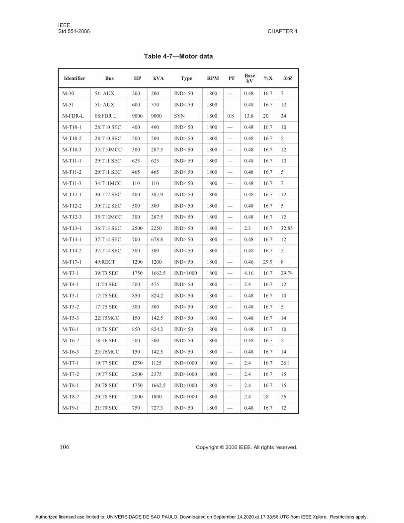
IEEEStd 551-2006 CHAPTER 4
106 Copyright © 2006 IEEE. All rights reserved.
Table 4-7—Motor data
Identifier Bus HP kVA Type RPM PFBase kV
%X X/R
M-30 51: AUX 200 200 IND> 50 1800 — 0.48 16.7 7
M-31 51: AUX 600 570 IND< 50 1800 — 0.48 16.7 12
M-FDR-L 08:FDR L 9000 9000 SYN 1800 0.8 13.8 20 34
M-T10-1 28:T10 SEC 400 400 IND< 50 1800 — 0.48 16.7 10
M-T10-2 28:T10 SEC 500 500 IND> 50 1800 — 0.48 16.7 5
M-T10-3 33:T10MCC 300 287.5 IND< 50 1800 — 0.48 16.7 12
M-T11-1 29:T11 SEC 625 625 IND> 50 1800 — 0.48 16.7 10
M-T11-2 29:T11 SEC 465 465 IND< 50 1800 — 0.48 16.7 5
M-T11-3 34:T11MCC 110 110 IND< 50 1800 — 0.48 16.7 7
M-T12-1 30:T12 SEC 400 387.9 IND> 50 1800 — 0.48 16.7 12
M-T12-2 30:T12 SEC 500 500 IND< 50 1800 — 0.48 16.7 5
M-T12-3 35:T12MCC 300 287.5 IND< 50 1800 — 0.48 16.7 12
M-T13-1 36:T13 SEC 2500 2250 IND> 50 1800 — 2.3 16.7 32.85
M-T14-1 37:T14 SEC 700 678.8 IND> 50 1800 — 0.48 16.7 12
M-T14-2 37:T14 SEC 300 300 IND< 50 1800 — 0.48 16.7 5
M-T17-1 49:RECT 1200 1200 IND< 50 1800 — 0.46 29.9 8
M-T3-1 39:T3 SEC 1750 1662.5 IND>1000 1800 — 4.16 16.7 29.74
M-T4-1 11:T4 SEC 500 475 IND> 50 1800 — 2.4 16.7 12
M-T5-1 17:T5 SEC 850 824.2 IND< 50 1800 — 0.48 16.7 10
M-T5-2 17:T5 SEC 500 500 IND> 50 1800 — 0.48 16.7 5
M-T5-3 22:T5MCC 150 142.5 IND< 50 1800 — 0.48 16.7 14
M-T6-1 18:T6 SEC 850 824.2 IND< 50 1800 — 0.48 16.7 10
M-T6-2 18:T6 SEC 500 500 IND> 50 1800 — 0.48 16.7 5
M-T6-3 23:T6MCC 150 142.5 IND< 50 1800 — 0.48 16.7 14
M-T7-1 19:T7 SEC 1250 1125 IND>1000 1800 — 2.4 16.7 26.1
M-T7-2 19:T7 SEC 2500 2375 IND>1000 1800 — 2.4 16.7 15
M-T8-1 20:T8 SEC 1750 1662.5 IND>1000 1800 — 2.4 16.7 15
M-T8-2 20:T8 SEC 2000 1800 IND>1000 1800 — 2.4 28 26
M-T9-1 21:T9 SEC 750 727.3 IND< 50 1800 — 0.48 16.7 12
Authorized licensed use limited to: UNIVERSIDADE DE SAO PAULO. Downloaded on September 14,2020 at 17:33:56 UTC from IEEE Xplore. Restrictions apply.

CALCULATING SHORT-CIRCUIT CURRENTS FOR SYSTEMS IEEEWITHOUT AC DECAY Std 551-2006
Copyright © 2006 IEEE. All rights reserved. 107
Table 4-8—Transformer data
Identifier kVA %Z1X/R (+)
%Z0X/R (0)
kV Tap From bus To bus
T-1 15000 8 17 7.2 17 69 /13.8 69 01:69-1 03:MILL-1
T-2 15000 8 17 7.4 17 69 /13.8 69 02:69-2 04:MILL-2
T-3 1725 6 8 6 8 13.8/4.16 13.8 05:FDR F 39:T3 SEC
T-4 1500 5.5 6.5 5.5 6.5 13.8/2.4 13.8 06:FDR H 11:T4 SEC
T-5 1500 6.75 6.5 6.75 6.5 13.8/0.48 13.8 12:T5 PRI 17:T5 SEC
T-6 1500 5.75 6.5 5.75 6.5 13.8/0.48 13.8 13:T6 PRI 18:T6 SEC
T-7 3750 5.5 12 5.5 12 13.8/2.4 13.8 06:FDR H 19:T7 SEC
T-8 3750 5.5 12 5.5 12 13.8/2.4 13.8 15:FDR I 20:T8 SEC
T-9 750 5.75 5 5.5 5 13.8/0.48 13.8 16:T9 PRI 21:T9 SEC
T-10 1500 5.75 6.5 5.75 6.5 13.8/0.48 13.8 25:T10 PRI
28:T10 SEC
T-11 1500 5.75 6.5 5.5 6.5 13.8/0.48 13.8 26:FDR G 29:T11 SEC
T-12 1500 5.75 6.5 5.5 6.5 13.8/0.48 13.8 27:T12 PRI
30:T12 SEC
T-13 2500 5.75 10 50 10 13.8/2.4 13.8 31:FDR P 36:T13 SEC
T-14 1000 5.75 5.5 50 5.5 13.8/0.48 13.8 32:FDR Q 37:T14 SEC
T-17 1250 4.5 6 4.5 6 13.8/0.48 13.8 05:FDR F 49:RECT
T-18 1500 5.75 5.91 5.75 5.91 13.8/0.48 13.8 50:GEN1 51:AUX
Table 4-9—Current-limiting reactor data
Identifier Through kVA Amps Ohms Material kV %Z X/R Bus
CLL-3 23903 1000.0 0.8 Copper 13.8 3.35 100 04:MILL-2
Authorized licensed use limited to: UNIVERSIDADE DE SAO PAULO. Downloaded on September 14,2020 at 17:33:56 UTC from IEEE Xplore. Restrictions apply.

IEEEStd 551-2006 CHAPTER 4
108 Copyright © 2006 IEEE. All rights reserved.
Table 4-10—Cable data
IdentifierDescription
(kcmil)Material
Length(ft)
Length(m)
kV From bus To bus
C-E1 1-3/C-250 CU PVC 650 198.1 13.8 03:MILL-1 09:FDR E
C-E2 1-3/C-250 CU PVC 1833 558.7 13.8 09:FDR E 25:T10PRI
C-E3 1-3/C-250 CU PVC 75 22.9 13.8 09:FDR E 13:T6PRI
C-E4 1-3/C-250 CU PVC 165 50.3 13.8 09:FDR E 12:T5PRI
C-F1 1-3/C-250 CU PVC 325 99.1 13.8 03:MILL-1 05:FDR F
C-G1 1-3/C-250 CU PVC 680 207.3 13.8 03:MILL-1 26:FDR G
C-H1 1-3/C-250 CU PVC 471 143.6 13.8 03:MILL-1 06:FDR H
C-I1 1-3/C-250 CU PVC 980 298.7 13.8 04:MILL-2 15:FDR I
C-J2 1-3/C-250 CU PVC 619 188.7 13.8 04:MILL-2 27:T12 PRI
C-J3 1-3/C-250 CU PVC 1187 361.8 13.8 16:T9 PRI 04:MILL-2
C-J4 1-3/C-250 CU PVC 200 61 13.8 10:EMERG 13:T6 PRI
C-J5 1-3/C-250 CU Steel 10 3 13.8 10:EMERG 12:T5 PRI
C-J6 1-3/C-250 CU PVC 475 144.8 13.8 10:EMERG 27:T12 PRI
C-L1 1-3/C-400 CU PVC 510 155.4 13.8 04:MILL-2 08:FDR L
C-M1 1-3/C-250 CU PVC 510 155.4 13.8 04:MILL-2 24:FDR M
C-M2 1-3/C-250 CU PVC 340 103.6 13.8 24:FDR M 31:FDR P
C-M3 1-3/C-250 CU PVC 485 147.8 13.8 24:FDR M 32:FDR Q
C-T10-1 2-3/C-400 CU PVC 50 15.2 0.48 28:T10 SEC 38:480TIE
C-T10-2 1-3/C-250 CU PVC 20 6.1 0.48 33:T10MCC 28:T10SEC
C-T11-1 2-3/C-400 CU PVC 66 20.1 0.48 29:T11 SEC 38:480TIE
C-T11-2 1-3/C-250 CU PVC 20 6.1 0.48 34:T11MCC 29:T11SEC
C-T12-1 1-3/C-400 CU PVC 50 15.2 0.48 38:480 TIE 30:T12SEC
C-T12-2 1-3/C-250 CU PVC 20 6.1 0.48 35:T12MCC 30:T12SEC
C-T5-1 1-3/C-250 CU PVC 20 6.1 0.48 22:T5MCC 17:T5 SEC
C-T6-1 1-3/C-250 CU PVC 20 6.1 0.48 23:T6MCC 18:T6 SEC
C1A 2-1/C-500 CU PVC 2000 609.6 13.8 50:GEN1 03:MILL-1
Authorized licensed use limited to: UNIVERSIDADE DE SAO PAULO. Downloaded on September 14,2020 at 17:33:56 UTC from IEEE Xplore. Restrictions apply.

CALCULATING SHORT-CIRCUIT CURRENTS FOR SYSTEMS IEEEWITHOUT AC DECAY Std 551-2006
Copyright © 2006 IEEE. All rights reserved. 109
4.6.2 Per-unit data
The following tables summarize the raw data in the form of per-unit data on a 10 MVA
base. The utility system, generators, and motors have the impedances given in
Table 4-13 for the first cycle and interrupting time calculations. The branch data, also in
per-unit on a 10 MVA base, is shown in Table 4-14. Taken together, the data in these two
tables are for the complete system and will be used in this and subsequent chapters.
Table 4-11—Transmission line data
IdentifierDescrip-
tion(kcmil)
Material GMDLength
(mi)Length
(m)kV From bus To bus
L-1 266.8 ACSR 7.0 1.894 3048 69.0 100:UTIL-69 01:69-1
L-2 266.8 ACSR 7.0 1.894 3048 69.0 100:UTIL-69 02:69-2
Table 4-12—Busway data
Identifier Manuf.Length
(ft)Length
(m)Amps kV R X Mat.
From bus
To bus
BWY-1 SQD-I-Li 50.0 15.2 1000 0.48 0.0008 0.0005 CU 28:T10SEC
41:LGTS
Table 4-13—Per-unit source (utility, generator, and motor)
(per-unit on 10 MVA base)
First cycle Interrupting
Bus Description R X R X
100:UTIL-69 Util. 0.00045 0.00999 0.00045 0.00999
04:MILL-2 Gen. 0.00287 0.1024 0.00287 0.1024
50:GEN1 Gen. 0.00192 0.07168 0.00192 0.07168
51: AUX Med Ind 1.43143 10.02 3.57858 25.05
51: AUX Sm Ind 0.40773 4.89278 — —
08:FDR L Syn Mot 0.00654 0.22222 0.00981 0.33333
28:T10 SEC Sm Ind 0.69722 6.97225 — —
28:T10 SEC Med Ind 0.8016 4.008 2.004 10.02
Authorized licensed use limited to: UNIVERSIDADE DE SAO PAULO. Downloaded on September 14,2020 at 17:33:56 UTC from IEEE Xplore. Restrictions apply.

IEEEStd 551-2006 CHAPTER 4
110 Copyright © 2006 IEEE. All rights reserved.
33:T10MCC Sm Ind 0.8084 9.70071 — —
29:T11 SEC Med Ind 0.32064 3.2064 0.8016 8.016
29:T11 SEC Sm Ind 1.19953 5.99764 — —
34:T11MCC Sm Ind 3.62195 25.35361 — —
30:T12 SEC Med Ind 0.43055 5.16656 1.07637 12.91641
30:T12 SEC Sm Ind 1.11556 5.5778 — —
35:T12MCC Sm Ind 0.8084 9.70071 — —
36:T13 SEC Med Ind 0.0249 0.818 0.06225 2.04501
37:T14 SEC Med Ind 0.24602 2.95232 0.61506 7.38081
37:T14 SEC Sm Ind 1.85928 9.29634 — —
49:RECT Sm Ind 0.47769 3.82154 — —
39:T3 SEC Lg Ind 0.03378 1.0045 0.05067 1.50675
11:T4 SEC Med Ind 0.35158 4.21892 0.87894 10.54731
17:T5 SEC Sm Ind 0.33836 3.38359 — —
17:T5 SEC Med Ind 0.8016 4.008 2.004 10.02
22:T5MCC Sm Ind 1.39794 19.5711 — —
18:T6 SEC Sm Ind 0.33836 3.38359 — —
18:T6 SEC Med Ind 0.8016 4.008 2.004 10.02
23:T6MCC Sm Ind 1.39794 19.5711 — —
19:T7 SEC Lg Ind 0.05688 1.48446 0.08532 2.22669
19:T7 SEC Lg Ind 0.04688 0.70315 0.07032 1.05472
20:T8 SEC Lg Ind 0.06697 1.0045 0.10046 1.50675
20:T8 SEC Lg Ind 0.05983 1.55557 0.08975 2.33335
21:T9 SEC Sm Ind 0.31955 3.83474 — —
Table 4-13—Per-unit source (utility, generator, and motor)
(per-unit on 10 MVA base) (continued)
First cycle Interrupting
Bus Description R X R X
Authorized licensed use limited to: UNIVERSIDADE DE SAO PAULO. Downloaded on September 14,2020 at 17:33:56 UTC from IEEE Xplore. Restrictions apply.

CALCULATING SHORT-CIRCUIT CURRENTS FOR SYSTEMS IEEEWITHOUT AC DECAY Std 551-2006
Copyright © 2006 IEEE. All rights reserved. 111
Table 4-14—Per-unit impedances for all branches
From bus To bus R X Equipment description
01:69-1 03:MILL-1 0.00313 0.05324 Transf T-1
02:69-2 04:MILL-2 0.00313 0.05324 Transf T-2
05:FDR F 39:T3 SEC 0.04314 0.34514 Transf T-3
06:FDR H 11:T4 SEC 0.05575 0.3624 Transf T-4
12:T5 PRI 17:T5 SEC 0.06843 0.44477 Transf T-5
13:T6 PRI 18:T6 SEC 0.05829 0.37888 Transf T-6
06:FDR H 19:T7 SEC 0.14616 0.14616 Transf T-7
15:FDR I 20:T8 SEC 0.14616 0.14616 Transf T-8
16:T9 PRI 21:T9 SEC 0.15036 0.75178 Transf T-9
25:T10 PRI 28:T10 SEC 0.05829 0.37888 Transf T-10
26:FDR G 29:T11 SEC 0.05829 0.37888 Transf T-11
27:T12 PRI 30:T12 SEC 0.05829 0.37888 Transf T-12
31:FDR P 36:T13 SEC 0.02289 0.22886 Transf T-13
32:FDR Q 37:T14 SEC 0.10286 0.56573 Transf T-14
05:FDR F 49:RECT 0.05918 0.3551 Transf T-17
50:GEN1 51: AUX 0.06391 0.37797 Transf T-18
03:MILL-1 09:FDR E 0.0015 0.00125 Cable C-E1
09:FDR E 25:T10 PRI 0.00424 0.00353 Cable C-E2
09:FDR E 13:T6 PRI 0.00017 0.00014 Cable C-E3
09:FDR E 12:T5 PRI 0.00038 0.00032 Cable C-E4
03:MILL-1 05:FDR F 0.00075 0.00063 Cable C-F1
03:MILL-1 26:FDR G 0.00157 0.00131 Cable C-G1
03:MILL-1 06:FDR H 0.00109 0.00091 Cable C-H1
04:MILL-2 15:FDR I 0.00227 0.00189 Cable C-I1
04:MILL-2 27:T12 PRI 0.00143 0.00119 Cable C-J2
16:T9 PRI 04:MILL-2 0.00275 0.00229 Cable C-J3
10:EMERG 13:T6 PRI 0.00046 0.00039 Cable C-J4
10:EMERG 12:T5 PRI 0.00002 0.00002 Cable C-J5
10:EMERG 27:T12 PRI 0.0011 0.00091 Cable C-J6
Authorized licensed use limited to: UNIVERSIDADE DE SAO PAULO. Downloaded on September 14,2020 at 17:33:56 UTC from IEEE Xplore. Restrictions apply.

IEEEStd 551-2006 CHAPTER 4
112 Copyright © 2006 IEEE. All rights reserved.
4.6.3 Computer short-circuit printout
In this subclause, sample computer-generated results are provided. These results are not
intended to be complete. Rather, they are intended to provide a sample of the type of data
that is produced by a wide variety of commercially-available short-circuit programs.
Because of the built-in assumptions that many programs make, these samples should not
be used for benchmarking purposes.
FAULT LEVEL IN KILOAMPS
***** BUS: 100 :UTIL-69 *****
8.367 KA AT -87.42 DEG ( 999.99 MVA): X/R = 22.20 KV = 69.000
Ze = 0.0004503 +j 0.0099900 (Complex)
SYM kA*1.6 = 13.39 ASYM kA Based on X/R ratio = 13.27 kA
CONTRIBUTIONS TO FAULT:
BUS to BUS MAG ANG BUS to BUS MAG ANG
UTIL 100:UTIL69 8.367 ???42 01:69-1 100:UTIL69 0.000 -3.70
02:69-2 100:UTIL69 0.000 ???00
04:MILL-2 08:FDR L 0.00076 0.00092 Cable C-L1
04:MILL-2 24:FDR M 0.00118 0.00098 Cable C-M1
24:FDR M 31:FDR P 0.00079 0.00065 Cable C-M2
24:FDR M 32:FDR Q 0.00112 0.00093 Cable C-M3
28:T10 SEC 38:480 TIE 0.03039 0.02929 Cable C-T10-1
33:T10MCC 28:T10 SEC 0.03813 0.0245 Cable C-T10-2
29:T11 SEC 38:480 TIE 0.04012 0.03866 Cable C-T11-1
34:T11MCC 29:T11 SEC 0.03813 0.0245 Cable C-T11-2
38:480 TIE 30:T12 SEC 0.06079 0.05858 Cable C-T12-1
35:T12MCC 30:T12 SEC 0.03813 0.0245 Cable C-T12-2
22:T5MCC 17:T5 SEC 0.03813 0.0245 Cable C-T5-1
23:T6MCC 18:T6 SEC 0.03813 0.0245 Cable C-T6-1
50:GEN1 03:MILL-1 0.00122 0.00243 Cable C1A
100:UTIL-69 01:69-1 0.00139 0.00296 T-Line L-1
100:UTIL-69 02:69-2 0.00139 0.00296 T-Line L-2
28:T10 SEC 41:LGTS 0.03429 0.02094 Bwy-1
Table 4-14—Per-unit impedances for all branches (continued)
From bus To bus R X Equipment description
Authorized licensed use limited to: UNIVERSIDADE DE SAO PAULO. Downloaded on September 14,2020 at 17:33:56 UTC from IEEE Xplore. Restrictions apply.

CALCULATING SHORT-CIRCUIT CURRENTS FOR SYSTEMS IEEEWITHOUT AC DECAY Std 551-2006
Copyright © 2006 IEEE. All rights reserved. 113
***** BUS: 01:69-1 *****
6.397 KA AT -81.91 DEG ( 764.53 MVA): X/R = 7.04 KV = 69.000
Ze = 0.0018405 +j 0.0129498 (Complex)
SYM kA*1.6 = 10.24 ASYM kA Based on X/R ratio = 8.70 kA
CONTRIBUTIONS TO FAULT:
BUS to BUS MAG ANG BUS to BUS MAG ANG
01:69-1 03:MILL-1 -0.000 -3.37 01:69-1 100:UTIL69 -6.397 -81.91
***** BUS: 02:69-2 *****
6.397 KA AT -81.91 DEG ( 764.52 MVA): X/R = 7.04 KV = 69.000
Ze = 0.0018403 +j 0.0129500 (Complex)
SYM kA*1.6 = 10.24 ASYM kA Based on X/R ratio = 8.70 kA
CONTRIBUTIONS TO FAULT:
BUS to BUS MAG ANG BUS to BUS MAG ANG
02:69-2 04:MILL-2 0.000 0.00 02:69-2 100:UTIL69 -6.397 -81.91
***** BUS: 03:MILL-1 *****
6.303 KA AT -85.69 DEG ( 150.66 MVA): X/R = 13.32 KV = 13.800
Ze = 0.0049843 +j 0.0661870 (Complex)
SYM kA*1.6 = 10.09 ASYM kA Based on X/R ratio = 9.48 kA
BUS to BUS MAG ANG BUS to BUS MAG ANG
CONTRIBUTIONS TO FAULT:
BUS to BUS MAG ANG BUS to BUS MAG ANG
01:69-1 03:MILL-1 6.303 -85.71 03:MILL-1 09:FDR E -0.001 0.11
03:MILL-1 05:FDR F 0.000 0.00 03:MILL-1 26:FDR G 0.000 0.00
03:MILL-1 06:FDR H 0.000 0.00 03:MILL-1 50:GEN1 0.000 0.00
4.7 Conclusions
In this chapter, the most basic short-circuit calculation techniques have been presented.
While only calculations that do not consider ac decay (NACD) have been considered, the
basic techniques and methods apply to the more complex calculations that are the subject
of future chapters. The data provided for the example system has been presented in its
entirety, and this data will be used extensively in subsequent chapters. The calculation
techniques for balanced three-phase faults with no ac decay have been demonstrated with
“hand” examples, and a brief sample of the types of results available from standard
commercial-grade short-circuit programs has been provided for informative purposes.
Authorized licensed use limited to: UNIVERSIDADE DE SAO PAULO. Downloaded on September 14,2020 at 17:33:56 UTC from IEEE Xplore. Restrictions apply.

IEEEStd 551-2006 CHAPTER 4
114 Copyright © 2006 IEEE. All rights reserved.
4.8 Bibliography
[B1] IEC 909:1977, German National Committee Report No. 73: Short-Circuit Currents.2
[B2] IEEE Std 399™-1997, IEEE Recommended Practices for Power System Analysis
(IEEE Brown Book).3, 4
[B3] IEEE Std C37.010™-1999 (Reaff 2005), IEEE Guide for AC High-Voltage Circuit
Breakers Rated on a Symmetrical Current Basis.
2IEC publications are available from the Sales Department of the International Electrotechnical Commission,Case Postale 131, 3, rue de Varembé, CH-1211, Genève 20, Switzerland/Suisse (http://www.iec.ch/). IEC publi-cations are also available in the United States from the Sales Department, American National Standards Institute,11 West 42nd Street, 13th Floor, New York, NY 10036, USA.3IEEE publications are available from the Institute of Electrical and Electronics Engineers, 445 Hoes Lane, P.O.Box 1331, Piscataway, NJ 08855-1331, USA (http://standards.ieee.org/).4The IEEE standards or products referred to in this subclause are trademarks of the Institute of Electrical andElectronics Engineers, Inc.
Authorized licensed use limited to: UNIVERSIDADE DE SAO PAULO. Downloaded on September 14,2020 at 17:33:56 UTC from IEEE Xplore. Restrictions apply.

Copyright © 2006 IEEE. All rights reserved. 115
Chapter 5 Calculating ac short-circuit currents for systems with contributions from synchronous machines
5.1 Introduction
This chapter describes the calculations of three-phase short-circuit currents for systems
with ac current decay from synchronous machines. This could be applicable to utilities
and larger industrial systems.
This chapter is limited to the consideration of short-circuit currents that occur under the
following conditions:
1) Short-circuit fault currents that occur in low-voltage ac systems and medium-
voltage ac systems operating at a constant frequency.
2) For the duration of the short circuit, there is no change in the source driving
voltage or voltages that caused the initial short-circuit current to flow.
3) The fault impedance is zero and has no current limiting effect.
4) Synchronous machine fault current contribution varies with time after the fault
and is not negligible.
5) For simplification, only three-phase faults will be considered. Unbalanced faults
are covered in a later chapter.
5.2 Purpose
The objective of this chapter is to give recommended standardized procedures for the
calculation of short-circuit currents on systems with ac decay from synchronous machines.
The application and selection of interrupting equipment based on the calculated fault
current on a total system is covered in Chapter 10. Fault currents with no ac fault current
decay are covered in Chapter 4 and fault currents from induction machines are covered in
Chapter 6. AC current decay calculations add a small amount of complexity to the no ac
decay fault calculations. The sample one-line diagram used to show the calculations is the
same as used in Chapter 4 except with synchronous machines added. Hand and computer
generated calculations will be made at several buses.
5.3 ANSI guidelines
The generator reactances used in this chapter will be based on the first cycle and
interrupting reactances as given in IEEE Std C37.010™-1999 [B3].1 The representation of
synchronous machines by a varying reactance is easily adapted to other analytical
techniques, such as IEC 909:1977 [B2]. Because of the decaying nature of the ac currents,
a first cycle and an interrupting time calculation may be needed for equipment evaluation.
1The numbers in brackets correspond to those of the bibliography in 5.12.
Authorized licensed use limited to: UNIVERSIDADE DE SAO PAULO. Downloaded on September 14,2020 at 17:33:56 UTC from IEEE Xplore. Restrictions apply.
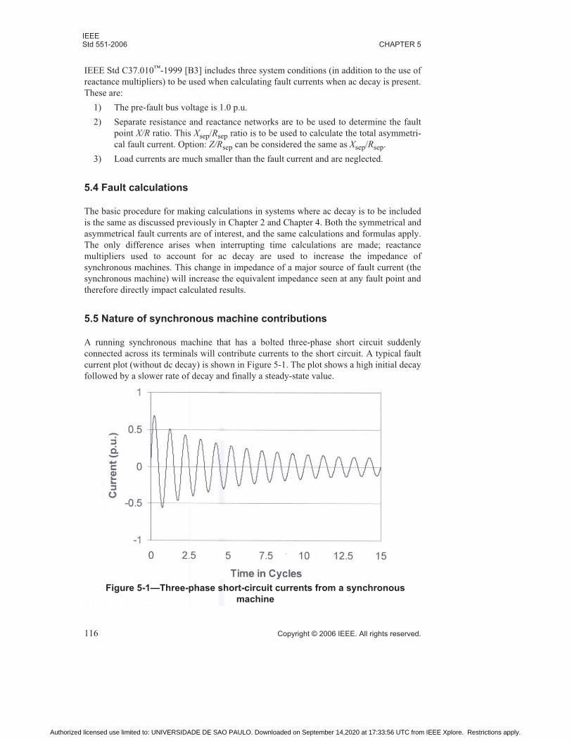
IEEEStd 551-2006 CHAPTER 5
116 Copyright © 2006 IEEE. All rights reserved.
IEEE Std C37.010™-1999 [B3] includes three system conditions (in addition to the use of
reactance multipliers) to be used when calculating fault currents when ac decay is present.
These are:
1) The pre-fault bus voltage is 1.0 p.u.
2) Separate resistance and reactance networks are to be used to determine the fault
point X/R ratio. This Xsep/Rsep ratio is to be used to calculate the total asymmetri-
cal fault current. Option: Z/Rsep can be considered the same as Xsep/Rsep.
3) Load currents are much smaller than the fault current and are neglected.
5.4 Fault calculations
The basic procedure for making calculations in systems where ac decay is to be included
is the same as discussed previously in Chapter 2 and Chapter 4. Both the symmetrical and
asymmetrical fault currents are of interest, and the same calculations and formulas apply.
The only difference arises when interrupting time calculations are made; reactance
multipliers used to account for ac decay are used to increase the impedance of
synchronous machines. This change in impedance of a major source of fault current (the
synchronous machine) will increase the equivalent impedance seen at any fault point and
therefore directly impact calculated results.
5.5 Nature of synchronous machine contributions
A running synchronous machine that has a bolted three-phase short circuit suddenly
connected across its terminals will contribute currents to the short circuit. A typical fault
current plot (without dc decay) is shown in Figure 5-1. The plot shows a high initial decay
followed by a slower rate of decay and finally a steady-state value.
Figure 5-1—Three-phase short-circuit currents from a synchronous
machine
Authorized licensed use limited to: UNIVERSIDADE DE SAO PAULO. Downloaded on September 14,2020 at 17:33:56 UTC from IEEE Xplore. Restrictions apply.

CALCULATING AC SHORT-CIRCUIT CURRENTS FOR SYSTEMS IEEEWITH CONTRIBUTIONS FROM SYNCHRONOUS MACHINES Std 551-2006
Copyright © 2006 IEEE. All rights reserved. 117
The short-circuit current decreases exponentially in time from an initially high value to a
lower steady-state level. This happens because the flux across the air gap of the
synchronous machine is much larger at the instant the short-circuit occurs than it is a few
cycles later. As the air-gap flux reduces because of limited field current capability, the
stator current decreases. The internal voltage generated by the air-gap flux determines the
magnitude of the short-circuit current. This changing air-gap flux accounts for the gradual
decrease in the short-circuit current as shown in Figure 5-1.
The rate of decay and the steady-state fault current depend upon the synchronous machine
time constants and the regulating action of the field current, if any. The initial current
contribution is caused by an internal stator driving voltage generated by trapped rotor field
flux. The current to the terminal short circuit is limited by the internal impedance of the
machine. The current in two or all three phases is asymmetrical at first, and consists of an
ac and a dc component.
The ac component decays because the rotor flux is not maintained by the normal applied
field voltage. The dc component, a transient not supported by any driving voltage, also
decays. The initial frequency of the fault current is the same as system frequency and is
directly related to rotor speed. Thereafter, the frequency of the fault current from a motor
reduces at a rate dependent on motor mechanical load and combined motor and load
inertia while those of a generator will increase based on the turbine power and combined
turbine and generator inertia. For the first few cycles after the short circuit, the frequency
change is usually conservatively considered to be inconsequential.
The equivalent circuit used to represent a synchronous machine or a group of synchronous
machines in simplified short-circuit calculations is shown in Figure 5-2. For calculations
based on Thevenin's theorem, the equivalent circuit of the complete system containing
several synchronous machines is reduced to a single driving voltage in series with an
equivalent impedance.
As described previously, the synchronous machine driving voltages are not constant. They
change with time depending on machine loading, excitation voltage, and system
conditions. The machine impedances depend upon the physical design of the machine and
are essentially constant. They do change with temperature and frequency.
Figure 5-2—Synchronous machine per phase equivalent circuit
~
E (Internal)Impedance of Machine Phase
Authorized licensed use limited to: UNIVERSIDADE DE SAO PAULO. Downloaded on September 14,2020 at 17:33:56 UTC from IEEE Xplore. Restrictions apply.

IEEEStd 551-2006 CHAPTER 5
118 Copyright © 2006 IEEE. All rights reserved.
One simplified calculation technique of increasing the reactance from X"dv in increments
as time passes after the short circuit is initiated accounts for the ac current decay,
assuming the voltage is constant. This model obtains the machine decaying ac current
contributions in the equivalent circuit without changing the circuit driving voltage. This
technique is widely used and accepted by the industry. Typical reactance multiplying
factors to be applied to X"dv depend on whether the synchronous machine is a generator or
a motor. Typical reactance multiplying factors are given in Table 5-1. Definitions of
synchronous machine reactance are given in Chapter 1 and reviewed in this chapter.
The initial magnitude of the ac component is calculated using the subtransient reactance
X"dv of the machine. The initial magnitude of the dc component for short-circuit
calculations is equal to the crest value of the initial ac component, assuming the fault
current in one phase has the maximum possible asymmetry. Depending on the
synchronous machine time constants, the transition of fault current from subtransient to
transient to synchronous will vary and will generally take longer to decay than an
induction motor current as described in Chapter 6. If the field to the machine remains
energized, then a steady-state fault current will exist due to continuous replenishing of
stator flux energy that is removed by the fault. Otherwise, the fault current from a
synchronous machine will decay to zero.
Typical reactances of synchronous motors when the actual reactance is not available are
given in Table 5-2.
Table 5-1—Synchronous machine reactances and multiplying factors from
IEEE Std C37.010 [B3] and IEEE Std C37.13™ [B2]
Type of machineMedium voltage and
high voltage perIEEE Std C37.010
Low voltage per IEEE Std C37.13
First cycle calculations
Remote utility 1.0 × Xs 1.0 × Xs
Local generator 1.0 × X"dv 1.0 × X"dv
Synchronous motor 1.0 × X"dv 1.0 × X"dv
Interrupting time calculations (3–5 cycles)
Remote utility 1.0 × Xsa
a3–5 cycle interrupting times do not apply to low-voltage breakers.
Local generator 1.0 × X"dva
Synchronous motor 1.5 × X"dva
Authorized licensed use limited to: UNIVERSIDADE DE SAO PAULO. Downloaded on September 14,2020 at 17:33:56 UTC from IEEE Xplore. Restrictions apply.

CALCULATING AC SHORT-CIRCUIT CURRENTS FOR SYSTEMS IEEEWITH CONTRIBUTIONS FROM SYNCHRONOUS MACHINES Std 551-2006
Copyright © 2006 IEEE. All rights reserved. 119
Most synchronous machines fall into one of the following three categories:
1) Synchronous generators
2) Synchronous condensers
3) Synchronous motors
Synchronous generators are a principal source of electrical energy in power systems
because almost all utilities use synchronous generators to generate electricity. Many of the
larger industrial systems may include generators for energy conservation such as in
co-generation.
Synchronous condensers are used as a means of reducing power system transmission
losses, reactive power control and controlling voltages in a transmission or distribution
system. They are connected to the power system as a motor but are neither connected to a
load nor to a prime mover. Modern equipment such as static var compensators (SVCs) are
much more common today than synchronous condensers, but the older rotating
compensators may still be occasionally encountered in practice.
Synchronous motors are generally used to drive large loads such as compressors, pumps,
and M-G sets and to supply capacitive power for power factor improvement. Sometimes
synchronous motors are operated near unity power factor and rarely are operated drawing
reactive power from system. The motors can have fixed or constant current fields or can
have regulators that control bus voltage or motor power factor.
5.6 Synchronous machine reactances
Synchronous machines have a number of reactances and time constants that can be used
when modeling the machine. For short-circuit studies, these normally are reduced to the
following:
1) X"dv – Subtransient reactance (saturated)
2) X'dv – Transient reactance (saturated)
3) Xd – Synchronous reactance (saturated)
4) X2v – Negative sequence reactance (saturated)
5) X0v – Zero sequence reactance (saturated)
6) Ta3 – Three-phase short-circuit time constant
7) T"do, T'do – Subtransient and transient time constants
Table 5-2—Synchronous machine typical reactances
Number of poles 60 Hz RPM X"dv reactance
> 16 ≤ 450 28%
8–14 514–900 20%
2–6 ≥ 1200 15%
Authorized licensed use limited to: UNIVERSIDADE DE SAO PAULO. Downloaded on September 14,2020 at 17:33:56 UTC from IEEE Xplore. Restrictions apply.

IEEEStd 551-2006 CHAPTER 5
120 Copyright © 2006 IEEE. All rights reserved.
The definitions are as follows:
a) Direct-axis saturated subtransient reactance (X"dv) is the apparent reactance of the
stator winding at the instant short-circuit occurs with the machine at rated voltage,
no load. This reactance determines the current flow during the first few cycles
after short-circuit initiation.
b) Direct-axis saturated transient reactance (X'dv) is the apparent reactance of the
stator winding several cycles after initiation of the fault with the machine at rated
voltage, no load. The time period for which the reactance may be considered X'dv
can be up to a half (1/2) second or longer, depending upon the design of the
machine and is determined by the machine direct-axis transient time constant.
c) Direct-axis synchronous reactance Xd is the ratio of the fundamental-frequency
component of reactive armature voltage (Vd) to the fundamental-frequency direct-
axis positive-sequence component of armature current (I1d) under sustained
balanced conditions with rated field current applied.
d) Negative sequence reactance is the apparent reactance determined by placing a
line-to-line fault on the terminal of the generator at rated voltage. The negative
sequence reactance is calculated knowing the direct-axis reactances by
symmetrical components.
e) Zero sequence reactance is the apparent reactance determined by placing a line-to-
ground fault on the terminal of the generator so that rated current flows. Test are
done at reduced voltage. The zero sequence reactance is calculated using the
direct-axis and negative sequence reactances and symmetrical components.
f) Three-phase short-circuit armature time constant is the time required for the ac
short-circuit current to decay to 36.8% of its initial value. This time constant is a
combination of the subtransient and transient time constants.
g) Subtransient and Transient time constants are the times required for the respective
components of subtransient and transient currents to decay to 36.8% of their initial
value.
The most important characteristics of synchronous machines when calculating short-
circuit currents are the internal reactances and resistances. In practice, a single machine
reactance is assumed to vary (with time) from a subtransient to a transient to a sustained or
steady-state impedance; these variations control the ac component of the fault current. The
resistance controls the dc rate of decay. The machine time constants that determine the
rate of ac decay of the components of current are also important.
Expression of the synchronous machine variable reactance at any instant requires a
complicated formula involving time as one of the variables. However, for the sake of
simplicity the reactance is considered fixed over the time interval for which the fault
current is calculated. An expression of the ac rms current verses time for a three-phase
short-circuit at the terminals of a synchronous machine is as follows in Equation (5.1):
(5.1)
where t is in seconds and voltage and reactances are (typically) in per-unit.
IscE
Xdv″
--------E
Xdv′
--------–� �� �� �
e
tTdo
″--------–
EXdv
′--------
EXdv
--------–� �� �� �
e
tTdo
′--------–
EXd-----+ +=
Authorized licensed use limited to: UNIVERSIDADE DE SAO PAULO. Downloaded on September 14,2020 at 17:33:56 UTC from IEEE Xplore. Restrictions apply.

CALCULATING AC SHORT-CIRCUIT CURRENTS FOR SYSTEMS IEEEWITH CONTRIBUTIONS FROM SYNCHRONOUS MACHINES Std 551-2006
Copyright © 2006 IEEE. All rights reserved. 121
For a fault occurring away from the machine terminals, Equation (5.1) would have to
include the transfer impedance between the machine and the fault. In addition, the
resistance of the network would effect the decay time constants. Providing this detail in
short-circuit calculations would be very burdensome, thus the desire for simplicity while
maintaining conservatism.
5.7 One-line diagram data
The raw data, per-unit data, and one-line used is given in Chapter 4. The one-line diagram
from this chapter adds two generators, one at bus 04:MILL-2 and the other at bus
50:GEN1, and a large synchronous motor at bus 08:M-FDR-L. These are the decaying ac
fault sources along with the non-decaying utility source that provide short-circuit current
to a faulted bus.
5.8 Sample calculations
5.8.1 Sample calculation #1
In this example, a fault is placed on 2.4 kV bus 36:T13 SEC. The total impedance to the
fault is the reduction of all circuit and source impedances to the fault point. The total fault
impedance is affected by the synchronous machines connected to MILL-1 and MILL-2
buses. This reduces, as compared to the sample calculation in Chapter 4, the effective
impedance between the utility and MILL-2 bus and increases the fault level at bus 36:T13
SEC. Figure 5-3 provides a reduced one-line diagram showing the critical pieces of data
required. The impedance data needed for the network reduction is given in Chapter 4.
Equivalents need to be made for both a first cycle and an interrupting time calculation.
One equivalent is Generator 1 to the common connection point of bus 100:UTIL-69. The
connection would be 04:MILL-2 if the tie breaker 03:MILL-1 to 04:MILL-2 was closed.
The second equivalent is motor M-FDR L to bus 04:MILL-2. Because none of the other
motor sources are assumed to be connected, the equivalent source impedance in this case
is the sum of the series impedances between the machine internal source voltages and the
common connection points. The equivalent motor source impedance is provided on the
reduced one-line diagram. The actual series and parallel network reduction to obtain the
equivalents is not shown. The calculations for the fault current on bus 36:T13SEC are
given on following pages. The manual calculations provide the current magnitudes using
separate R and X network reductions while the computer printout uses the complex
network reduction for current and separate R and X network reductions for the X/R ratio.
In a system with sources that have a decaying ac component, both first cycle and
interrupting time calculations are required for the high-voltage buses. To accomplish both
sets of calculations, the source and equivalent impedances shown in Figure 5-3 are
required for both time periods. The cumulative impedance sums, down to the fault bus for
both first cycle and interrupting calculations, are shown in Table 5-3.
The symmetrical fault current via Trans T-13 is shown in Table 5-4.
Authorized licensed use limited to: UNIVERSIDADE DE SAO PAULO. Downloaded on September 14,2020 at 17:33:56 UTC from IEEE Xplore. Restrictions apply.

IEEEStd 551-2006 CHAPTER 5
122 Copyright © 2006 IEEE. All rights reserved.
Figure 5-3—Equivalents and impedance one-line diagram for sample
calculations
Authorized licensed use limited to: UNIVERSIDADE DE SAO PAULO. Downloaded on September 14,2020 at 17:33:56 UTC from IEEE Xplore. Restrictions apply.

CALCULATING AC SHORT-CIRCUIT CURRENTS FOR SYSTEMS IEEEWITH CONTRIBUTIONS FROM SYNCHRONOUS MACHINES Std 551-2006
Copyright © 2006 IEEE. All rights reserved. 123
5.9 Sample computer printout
In all cases of interest, computer programs are used that automatically provide the
impedance corrections for interrupting time calculations. A small sample of the results for
the example one-line (and system data) from Chapter 4 are given here for illustrative
purposes. As was the case in the examples in Chapter 4, the numerical values given here
are only intended to offer an idea of what is available from numerous commercially-
available short-circuit programs. Because different programs will make slightly different
modeling assumptions, particularly for data that is not available as input from the user, the
results given here should not be used for benchmarking purposes.
Table 5-3—R & X per-unit calculations for first cycle and interrupting time
First cycle Interrupting time
R X R X
Utility 0.00045 0.00999 0.00045 0.00999 (a)
Equiv. #1 0.00766 0.13031 0.00766 0.13031 (b)
Paralleling of the utility (a) with Equiv. #1 (b)
0.00043 0.00928 0.00043 0.00928 (c)
Line 0.00139 0.00296 0.00139 0.00296 (d)
Trans T-2 0.00313 0.05324 0.00313 0.05324 (e)
Add (c), (d), (e) 0.00495 0.06548 0.00495 0.06548 (f)
Generator #2 0.00287 0.10240 0.00287 0.10240 (g)
Equiv. #2 0.00730 0.22314 0.01057 0.33425 (h)
Parallel (f), Gen #2(g) with Equiv. #2 (h)
0.00145 0.03388 0.00155 0.03568 (i)
Cable C-M1 0.00118 0.00098 0.00118 0.00098 (j)
Add (i), (k) 0.00263 0.03486 0.00273 0.03666 (k)
Equiv. #3 999.999 9999.99 999.999 9999.99 (l)
Parallel (k) with Equiv. #3 (l) 0.00263 0.03486 0.00273 0.03666 (m)
Cable C-M2 0.00079 0.00065 0.00079 0.00065 (n)
Trans T-13 0.02289 0.22886 0.02289 0.22886 (o)
Add (m), (n), (o)(total impedance viewed through trans T-13)
0.02631 0.26437 0.02641 0.26617 (p)
Table 5-4—Calculations for fault current via trans T-13
First cycle Interrupting
I = MVAbase/(√ 3kV × Z) 9.0547 kA at 84.32º 8.9938 kA at 84.33º at 2.4 kV
X/R = 10.05 X/R = 10.08
Authorized licensed use limited to: UNIVERSIDADE DE SAO PAULO. Downloaded on September 14,2020 at 17:33:56 UTC from IEEE Xplore. Restrictions apply.
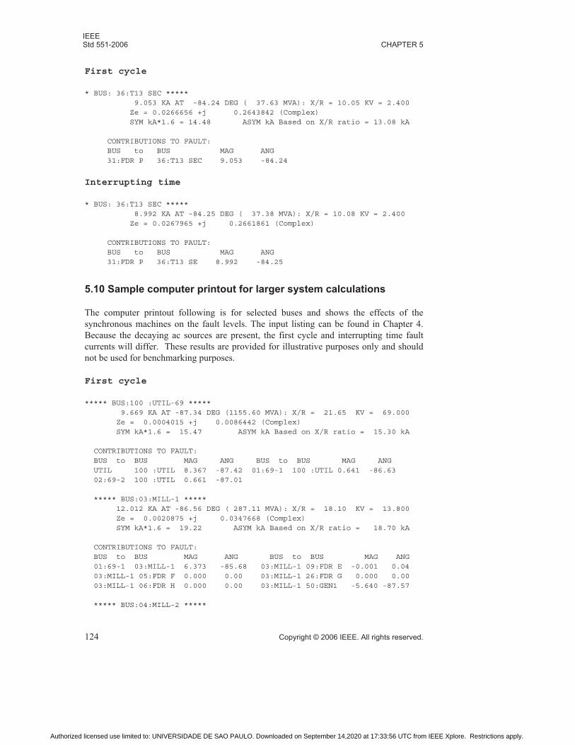
IEEEStd 551-2006 CHAPTER 5
124 Copyright © 2006 IEEE. All rights reserved.
First cycle
* BUS: 36:T13 SEC ***** 9.053 KA AT -84.24 DEG ( 37.63 MVA): X/R = 10.05 KV = 2.400 Ze = 0.0266656 +j 0.2643842 (Complex) SYM kA*1.6 = 14.48 ASYM kA Based on X/R ratio = 13.08 kA CONTRIBUTIONS TO FAULT: BUS to BUS MAG ANG 31:FDR P 36:T13 SEC 9.053 -84.24
Interrupting time
* BUS: 36:T13 SEC ***** 8.992 KA AT -84.25 DEG ( 37.38 MVA): X/R = 10.08 KV = 2.400 Ze = 0.0267965 +j 0.2661861 (Complex) CONTRIBUTIONS TO FAULT: BUS to BUS MAG ANG 31:FDR P 36:T13 SE 8.992 -84.25
5.10 Sample computer printout for larger system calculations
The computer printout following is for selected buses and shows the effects of the
synchronous machines on the fault levels. The input listing can be found in Chapter 4.
Because the decaying ac sources are present, the first cycle and interrupting time fault
currents will differ. These results are provided for illustrative purposes only and should
not be used for benchmarking purposes.
First cycle
***** BUS:100 :UTIL-69 ***** 9.669 KA AT -87.34 DEG (1155.60 MVA): X/R = 21.65 KV = 69.000 Ze = 0.0004015 +j 0.0086442 (Complex) SYM kA*1.6 = 15.47 ASYM kA Based on X/R ratio = 15.30 kA
CONTRIBUTIONS TO FAULT: BUS to BUS MAG ANG BUS to BUS MAG ANG UTIL 100 :UTIL 8.367 -87.42 01:69-1 100 :UTIL 0.641 -86.63 02:69-2 100 :UTIL 0.661 -87.01
***** BUS:03:MILL-1 ***** 12.012 KA AT -86.56 DEG ( 287.11 MVA): X/R = 18.10 KV = 13.800 Ze = 0.0020875 +j 0.0347668 (Complex) SYM kA*1.6 = 19.22 ASYM kA Based on X/R ratio = 18.70 kA
CONTRIBUTIONS TO FAULT: BUS to BUS MAG ANG BUS to BUS MAG ANG 01:69-1 03:MILL-1 6.373 -85.68 03:MILL-1 09:FDR E -0.001 0.04 03:MILL-1 05:FDR F 0.000 0.00 03:MILL-1 26:FDR G 0.000 0.00 03:MILL-1 06:FDR H 0.000 0.00 03:MILL-1 50:GEN1 -5.640 -87.57
***** BUS:04:MILL-2 *****
Authorized licensed use limited to: UNIVERSIDADE DE SAO PAULO. Downloaded on September 14,2020 at 17:33:56 UTC from IEEE Xplore. Restrictions apply.

CALCULATING AC SHORT-CIRCUIT CURRENTS FOR SYSTEMS IEEEWITH CONTRIBUTIONS FROM SYNCHRONOUS MACHINES Std 551-2006
Copyright © 2006 IEEE. All rights reserved. 125
12.326 KA AT -86.95 DEG ( 294.62 MVA): X/R = 23.29 KV = 13.800 Ze = 0.0018056 +j 0.0338942 (Complex) SYM kA*1.6 = 19.72 ASYM kA Based on X/R ratio = 19.63 kA
CONTRIBUTIONS TO FAULT: BUS to BUS MAG ANG BUS to BUS MAG ANG GEN 04:MILL-2 4.084 -88.39 02:69-2 04:MILL-2 6.371 -85.68 04:MILL-2 15:FDR I 0.000 0.00 04:MILL-2 16:T9 PRI 0.000 0.00 04:MILL-2 08:FDR L -1.874 -88.13 04:MILL-2 24:FDR M 0.000 0.00 04:MILL-2 27:T12 PRI 0.000 0.00
***** BUS:17:T5 SEC ***** 24.723 KA AT -81.44 DEG ( 20.55 MVA): X/R = 6.66 KV = 0.480 Ze = 0.0723980 +j 0.4811063 (Complex) SYM kA*1.6 = 39.56 ASYM kA Based on X/R ratio = 33.26 kA
CONTRIBUTIONS TO FAULT: BUS to BUS MAG ANG BUS to BUS MAG ANG 12:T5 PRI 17:T5 SEC 24.723 -81.44 17:T5 SEC 22:T5MCC 0.000 0.00
Interrupting time
***** BUS:100 :UTIL-69 ***** 9.629 KA AT -87.35 DEG (1150.80 MVA): X/R = 21.70 KV = 69.000 Ze = 0.0004020 +j 0.0086803 (Complex)
CONTRIBUTIONS TO FAULT: BUS to BUS MAG ANG BUS to BUS MAG ANG UTIL 100 :UTIL 8.367 -87.42 01:69-1 100 :UTIL 0.641 -86.63 02:69-2 100 :UTIL 0.621 -87.11
***** BUS:03:MILL-1 ***** 12.008 KA AT -86.57 DEG ( 287.02 MVA): X/R = 18.11 KV = 13.800 Ze = 0.0020873 +j 0.0347785 (Complex)
CONTRIBUTIONS TO FAULT: BUS to BUS MAG ANG BUS to BUS MAG ANG 01:69-1 03:MILL-1 6.369 -85.68 03:MILL-1 09:FDR E -0.001 -0.55 03:MILL-1 05:FDR F 0.000 0.00 03:MILL-1 26:FDR G 0.000 0.00 03:MILL-1 06:FDR H 0.000 0.00 03:MILL-1 50:GEN1 -5.640 -87.57
***** BUS:04:MILL-2 ***** 11.703 KA AT -86.89 DEG ( 279.73 MVA): X/R = 23.02 KV = 13.800 Ze = 0.0019365 +j 0.0356961 (Complex)
CONTRIBUTIONS TO FAULT: BUS to BUS MAG ANG BUS to BUS MAG ANG GEN 04:MILL-2 4.084 -88.39 02:69-2 04:MILL-2 6.371 -85.68 04:MILL-2 15:FDR I 0.000 0.00 04:MILL-2 16:T9 PRI 0.000 0.00 04:MILL-2 08:FDR L -1.251 -88.19 04:MILL-2 24:FDR M 0.000 0.00 04:MILL-2 27:T12 PRI 0.000 0.00
***** BUS:17:T5 SEC ***** 24.722 KA AT -81.44 DEG ( 20.55 MVA): X/R = 6.66 KV = 0.480 Ze = 0.0723978 +j 0.4811180 (Complex)
CONTRIBUTIONS TO FAULT:
Authorized licensed use limited to: UNIVERSIDADE DE SAO PAULO. Downloaded on September 14,2020 at 17:33:56 UTC from IEEE Xplore. Restrictions apply.

IEEEStd 551-2006 CHAPTER 5
126 Copyright © 2006 IEEE. All rights reserved.
BUS to BUS MAG ANG BUS to BUS MAG ANG
12:T5 PRI 17:T5 SEC 24.722 -81.44 17:T5 SEC 22:T5MCC 0.000 0.00
***** BUS:19:T7 SEC *****
13.181 KA AT -85.15 DEG ( 54.79 MVA): X/R = 11.92 KV = 2.400
Ze = 0.0154229 +j 0.1818492 (Complex)
CONTRIBUTIONS TO FAULT:
BUS to BUS MAG ANG
5.11 Conclusions
In this chapter, the techniques necessary for incorporating the effects of ac decay due to
synchronous machines have been presented. Through the use of simple reactance
multipliers, a straightforward extension of the basic calculation techniques of previous
chapters can be made to account for reduced fault currents supplied by synchronous
machines during time periods beyond the first cycle. The reactance modifiers presented
here are consistent with those in other relevant standards and provide conservative results.
The calculation approach has been demonstrated through “hand” calculations, and sample
computer results have been presented that show the capabilities of modern commercial
programs.
5.12 Bibliography
[B1] ANSI/NEMA Std Pub. No. MG1-2003, Motors and Generators, paragraph MG1-
1.58.2, 3
[B2] IEC 909:1977, German National Committee Report No. 73: Short-Circuit Currents.4
[B3] IEEE Std C37.010-1999 (Reaff 2005), IEEE Application Guide for AC High-Volt-
age Circuit Breakers Rated on a Symmetrical Current Basis.5, 6
[B4] IEEE Std C37.13-1990 (Reaff 1995), IEEE Standard for Low-Voltage AC Power
Circuit Breakers Used on Enclosures.
2ANSI publications are available from the Sales Department, American National Standards Institute, 25 West43rd Street, 4th Floor, New York, NY 10036, USA (http://www.ansi.org/).3NEMA publications are available from Global Engineering Documents, 15 Inverness Way East, Englewood, Colorado 80112, USA (http://global.ihs.com/).4IEC publications are available from the Sales Department of the International Electrotechnical Commission,Case Postale 131, 3, rue de Varembé, CH-1211, Genève 20, Switzerland/Suisse (http://www.iec.ch/). IEC publi-cations are also available in the United States from the Sales Department, American National Standards Institute,11 West 42nd Street, 13th Floor, New York, NY 10036, USA.5IEEE publications are available from the Institute of Electrical and Electronics Engineers, 445 Hoes Lane, P.O.Box 1331, Piscataway, NJ 08855-1331, USA (http://standards.ieee.org/).6The IEEE standards or products referred to in this subclause are trademarks of the Institute of Electrical andElectronics Engineers, Inc.
Authorized licensed use limited to: UNIVERSIDADE DE SAO PAULO. Downloaded on September 14,2020 at 17:33:56 UTC from IEEE Xplore. Restrictions apply.

Copyright © 2006 IEEE. All rights reserved. 127
Chapter 6Calculating ac short-circuit currents for systems with contributions from induction motors
6.1 Introduction
This chapter describes the calculations of three-phase short-circuit currents for systems
with ac current decay from induction motors. This could be applicable to many
commercial and industrial systems.
This chapter is limited to the consideration of short-circuit currents that occur under the
following conditions:
1) Short-circuit fault currents that occur in low-voltage ac systems and medium-
voltage ac systems operating at a constant frequency.
2) For the duration of the short circuit, there is no change in the source driving
voltage or voltages that caused the initial short-circuit current to flow.
3) The fault impedance is zero and has no current limiting effect.
4) Motor fault current contribution varies with time after the fault and is not
negligible.
5) For simplification, only three-phase faults will be considered. Unbalanced faults
are covered in Chapter 11.
6.2 Purpose
The objective of this chapter is to give recommended standardized procedures for the
calculation of short-circuit current on systems with ac decay from induction motors. The
application and selection of interrupting equipment based on the calculated fault current
are covered in Chapter 10. Fault currents with no ac fault current decay are covered in
Chapter 4 and fault currents from synchronous machines is covered in Chapter 5. AC
current decay calculations add a small amount of complexity to the no ac decay fault
calculations. The sample one-line diagram used to show the calculations is the same as
used for the previous calculations. Hand and computer generated calculations will be
made at several locations.
6.3 ANSI guidelines
The motor reactances used in this chapter will be based on the ratio of interrupting to first
cycle reactances as given in IEEE Std C37.010™-1999 [B4],1 IEEE Std C37.13™-1990
[B5], and an IEEE paper on induction motor contribution (Heuning [B2]). The
representation of induction motors by a varying reactance is easily adapted to other
analytical techniques, such as IEC 909:1988 [B3].
1The numbers in brackets correspond to those of the bibliography in 6.13.
Authorized licensed use limited to: UNIVERSIDADE DE SAO PAULO. Downloaded on September 14,2020 at 17:33:56 UTC from IEEE Xplore. Restrictions apply.

IEEEStd 551-2006 CHAPTER 6
128 Copyright © 2006 IEEE. All rights reserved.
IEEE Std C37.010-1999 [B4] includes three conditions, in addition to the condition listed
in section 6.1, to be used when calculating fault currents. These are as follows:
1) The pre-fault bus voltage is 1.0 p.u.
2) Separate resistance and reactance networks are to be used to determine the fault
point X/R ratio. This Xsep/Rsep ratio is to be used to calculate the total
asymmetrical fault current. Option: Z/Rsep can be considered the same as Xsep/
Rsep.
3) Load currents are much smaller than the fault current and neglected.
In IEEE Std C37.010-1999 [B4], several simplified methods are listed for use where the
current determined by an E/X calculation (instead of E/Z) meets specific fault current or
X/R ratio criteria. For example, when the fault current is less than 80% of the breaker duty,
an E/X calculation can be used. To determine if the current calculated by the simplified
methods meets these criteria, most of the effort that is needed for the detailed ANSI
calculation is already done. Because having several methods to calculate breaker duty
current could lead to confusion, the detailed ANSI calculation will be used here. Most
computer programs that follow the ANSI recommended method use the more detailed
ANSI procedure.
When induction motors are included in a system, the symmetrical ac component of the
short-circuit current varies based on the time after the fault. In Chapter 3, asymmetry was
discussed and was shown to depend on the fault point X/R ratio and the point on the
voltage sine wave at which the fault is initiated. A fault current flowing from energy
sources may be asymmetrical and have both an ac and dc component. The dc component
is a transient value and decays with time. In Chapter 2, several different theoretical and
empirical equations were given that relate the maximum peak and rms currents in the first
cycle to the ac symmetrical current. For the sample calculations in this chapter, the “Violet
Book” equations will be used and are repeated below.
The first cycle Violet Book equation is:
(6.1)
(6.2)
where τ = 0.49 – 0.1ε–(X/R)/3
Equation (2.3) can be rewritten to calculate the total current at other points in time.
(6.3)
Ipeak Iac, peak 1 e
4πτRX
-------------–
+� �� �� �
=
Irms Iac,rms
2 Idc
2+ Iac, rms 1 2e
4πτRX
-------------–
+= =
Irms Iac, rms 1 2e
4πtR2X
-------------–
+� �� �� �
=
Authorized licensed use limited to: UNIVERSIDADE DE SAO PAULO. Downloaded on September 14,2020 at 17:33:56 UTC from IEEE Xplore. Restrictions apply.
CALCULATING AC SHORT-CIRCUIT CURRENTS FOR SYSTEMS IEEEWITH CONTRIBUTIONS FROM INDUCTION MOTORS Std 551-2006
Copyright © 2006 IEEE. All rights reserved. 129
where t is in cycles at 60 Hz.
Equation (6.1) and Equation (6.2) can be used to calculate the maximum asymmetry
during the first cycle, while Equation (6.3) can be used for interrupting times greater than
1 cycle.
Peak currents are often associated with equipment rated less than 1000 V and rms currents
are used with the higher voltage equipment. See the tables in Chapter 2 for the comparison
of the approximation equation peaks to the actual peak. When equipment operating times
are given in cycles at a particular frequency, the time frequencies can be ratioed to 60 Hz.
Five cycles at 50 Hz is the same time as six cycles at 60 Hz.
The dc current decrement for a simple single circuit of one branch is an exponential decay.
In a multi-branch power system, a single X/R ratio is only an approximation. Each branch
will actually have its own time constant and the total current will decay at some rate that is
dependent on the combined effect. There is no single time constant that will exactly
describe the dc decrement of a multi-branch total fault current.
6.4 Fault calculations
Fault calculations can be done in per-unit or in ohms with transformer ratios taken into
account. The sample calculations used in this book will be shown using the per-unit
method. The steps in calculating ANSI fault currents are as follows:
1) Obtain an up-to-date one-line diagram.
2) Determine the impedance of each branch and source for the time period of
concern.
3) Reduce the network impedances to a single R and X using separate R and Xnetwork reductions.
4) Optional: Reduce the network impedances to a single R and X impedance using
separate R and complex impedance network reductions and calculate equivalent
X/R from Z/Rsep.
5) Calculate the fault current by combining the separate R and X fault point
impedance and treating the result as a complex impedance or by using the optional
complex impedance network impedance.
6) Calculate the fault point X/R ratio using the separate R and X network reduction
values.
7) Calculate any asymmetry currents, if required.
8) Calculate the branch contributions, if required.
6.5 Nature of induction motor contributions
A running induction motor that has a bolted three-phase short circuit suddenly connected
across its terminals will contribute currents to the short circuit. Typical fault current vs.
time plots are shown in Figure 6-1. The plot shows a high initial current decay followed by
fairly rapid decay to zero.
Authorized licensed use limited to: UNIVERSIDADE DE SAO PAULO. Downloaded on September 14,2020 at 17:33:56 UTC from IEEE Xplore. Restrictions apply.

IEEEStd 551-2006 CHAPTER 6
130 Copyright © 2006 IEEE. All rights reserved.
The current contribution is caused by a stator driving voltage generated by trapped rotor
flux. The current to the terminal short circuit is limited by the internal reactance of the
motor. The current in two or all three phases is asymmetrical at first, and that each offset
current consists of an ac and a dc component. The ac component decays because the rotor
flux is not maintained by normal applied voltage. The dc component, a transient not
supported by any driving voltage, also decays. The frequency differs initially from system
frequency by motor slip and thereafter reduces at a rate dependent on motor mechanical
load and combined motor and load inertia. For the first few cycles after the short circuit,
the frequency change is usually conservatively considered to be inconsequential.
The initial magnitude of the ac component is calculated using the subtransient motor
reactance X". It is accepted practice to substitute the known or estimated locked rotor
reactance XLR for X". The initial magnitude of dc component for short-circuit calculations
is taken to be equal to the crest value of the initial ac component. This is based on the
conservative assumption that the current in one of the phases will have the maximum
possible asymmetry.
The equivalent circuit used to represent an induction motor or a group of induction motors
with similar characteristics in simplified short-circuit calculations is shown in Figure 6-2.
For calculations based on Thevenin’s theorem, the equivalent circuit of the complete
system uses a single induction motor reactance that represents motors of different decays.
The individual induction motor voltage sources disappear by incorporation into the
Thevenin equivalent single driving voltage. For a fault calculation involving different
times after the fault, a different equivalent motor reactance would result because induction
motor equivalent reactances vary considerably with the motor size and speed.
Figure 6-1—Three-phase short-circuit currents from an induction motor
(vertical axis represents current; horizontal axis represents time)
Authorized licensed use limited to: UNIVERSIDADE DE SAO PAULO. Downloaded on September 14,2020 at 17:33:56 UTC from IEEE Xplore. Restrictions apply.

CALCULATING AC SHORT-CIRCUIT CURRENTS FOR SYSTEMS IEEEWITH CONTRIBUTIONS FROM INDUCTION MOTORS Std 551-2006
Copyright © 2006 IEEE. All rights reserved. 131
As indicated earlier, the ac component fault current from an induction motor will decay
with time. A simplified calculation technique accounts for the ac component current decay
by increasing the reactance from X" in increments as time passes after the short circuit
starts. This approach has the advantage of obtaining the correct value of ac fault current
while keeping the driving point voltage constant. Keeping the driving point voltage
constant simplifies the calculation process by allowing complex power systems to be
reduced to a simpler equivalent circuit. This technique is widely used and accepted by the
industry. The multipliers used to increase the reactance depend on the induction motor
horsepower, motor type and speed. Table 6-2 provides the recommended multipliers.
Short circuits are calculated frequently for fault points separated from contributing
induction motor terminals by series impedances. For simplified calculations, the same
reactance multiplying factors are applied to motor reactances whether the fault point is
close to, or remote from, the motor terminals. This is ideal for simplifying short-circuit
studies of large systems, usually performed by computer, because the set of equivalent
circuit impedances does not change as the fault point is relocated to calculate duties for
many buses.
In actual power systems, the voltage at a motor during a remote short circuit may be
partially sustained by nearer power sources. Initially, the voltage is depressed by the fault
and the motor generates a short-circuit current contribution. During the fault any partially
sustained voltage, if high enough, returns the motor to normal motoring function at less
than normal voltage. The simplified short-circuit calculation methods ignore this effect
and assume that all connected medium and large size motors, no matter how remote,
continue to contribute current to short circuits for at least four cycles after the short circuit
starts. However, due to this network action and a higher total equivalent impedance
between the remote motors and the fault, the remote motors contribution is less than it
would be for a terminal fault.
The reactance multiplying factors that increase with time account for partial decay but not
possibly complete disappearance of the motor contribution.
Figure 6-2—Induction motor per phase equivalent circuit
Authorized licensed use limited to: UNIVERSIDADE DE SAO PAULO. Downloaded on September 14,2020 at 17:33:56 UTC from IEEE Xplore. Restrictions apply.

IEEEStd 551-2006 CHAPTER 6
132 Copyright © 2006 IEEE. All rights reserved.
For longer times after the short circuit, appreciably after four cycles, smaller induction
motors are usually omitted from the equivalent circuit because induction motor fault
current contribution decay is rapid and approaching zero although the motors remain
connected. In addition, some motors nearer the fault may have been disconnected by
relays or contactor dropout on depressed voltage due to the nearby fault. The motor drop-
out effect could be included in interrupting time calculations. However, for a conservative
short-circuit current, often it is assumed that the motors do not drop out.
6.6 Large induction motors with prolonged contributions
When one or several large induction motors might appreciably affect the total short-circuit
current at a given bus, better accuracy is obtained by calculating motor current at
particular times of interest after the short circuit starts (for example, at first cycle and at
contact-parting times for medium-voltage circuit breakers). ANSI-approved guides for ac
medium-voltage circuit breakers suggest this in a note to the rotating machine reactance
table.
Both ac and dc components of motor current (Iac and Idc) are evaluated as time variables
assuming the decays from initial magnitudes are exponential, using Equation (6.4) and
Equation (6.5):
(6.4)
and
(6.5)
Time t is in cycles at system frequency, and Td" and Ta are the frequently used “X/R ratio”
time constants in radians at the same frequency. The time constant in radians for the ac
component decay Td" is X"/RR where RR is the rotor resistance (perhaps modified
slightly), and the time constant in radians for the dc component decay Ta is X"/RS where
RS is the stator resistance (again perhaps modified slightly).
The specified value of Ta is the same as the “X/R ratio” used in ANSI-approved standard
calculations of short-circuit duties for ac high-voltage circuit breakers.
Note that the tangent of the locked rotor impedance angle is less than, and does not
substitute for, the ANSI “X/R ratio.” The locked rotor impedance has more resistance than
the resistance used for short-circuit calculations. By definition, RS is the resistance
determining the time constant of the dc component decay. Since the motor dc component
currents are varying transiently, this is not the simple dc resistance that applies to the
decaying dc currents and the stator ac resistance is often used as a conservative
approximation.
Iac
EZ″-----� �� � e
2πtTd
″--------–
=
Idc 2 EZ″-----� �� � e
2πtTa
--------
=
Authorized licensed use limited to: UNIVERSIDADE DE SAO PAULO. Downloaded on September 14,2020 at 17:33:56 UTC from IEEE Xplore. Restrictions apply.

CALCULATING AC SHORT-CIRCUIT CURRENTS FOR SYSTEMS IEEEWITH CONTRIBUTIONS FROM INDUCTION MOTORS Std 551-2006
Copyright © 2006 IEEE. All rights reserved. 133
Many motor manufacturers are able to provide Td" and Ta values for specific important
motors, determined according to definitions in ANSI/NEMA Std MG1-1.58 [B1].
For more accurate calculations assuming exponential variations, moving the fault from the
motor terminals to insert external impedance in series with the motor reactance affects
both the short-circuit current initial magnitude and the time constants. For a series external
impedance Ze = Re + jXe, current magnitudes are found by substitution (Z" + Ze) for Z",
the ac time constant Td becomes (X" + Xe)/RR and the dc time constant becomes (X" + Xe)/
(RS + Re).
When the external circuit from the motor to the fault is more complicated than a single
impedance in series with the motor, calculations as just described are usually impractical
and simplified calculations are normally used. The simplified calculations are, however,
sometimes modified as suggested in ANSI-approved guides. For each large motor with a
significant short-circuit contribution, and for each desired specific calculation time ts after
the short-circuit starts, it is suggested that a special reactance multiplying factor be used in
simplified calculations for the motor instead of the standard factor listed in Table 6-1. The
special reactance factor suggested is ε+ts/Td", with ts and td" both in the same time units
(same as the reciprocal of ε–2πts/Td" used for current, with ts in cycles and Td" in radians,
same frequency).
For a particularly important bus with large induction motors, combining simplified and
more accurate procedures improves the quality of the results. With the motors omitted, the
simplified calculation determines the contribution of the rest of the system to the bus
short-circuit duty. The motor contribution is separately calculated by the more accurate
procedure. Then the ac and dc components of the contributions are separately added and
combined to obtain the final result.
6.7 Data accuracy
Data accuracy requirements are a function of motor size. The best possible data should be
sought for larger motors that have the highest influence on short-circuit study results. For
small motor groups, using first cycle Z" = 0.28 per-unit impedance as typical is probably
sufficiently conservative. Individual representation of large and medium motors (or
separate groups of medium motors) is normally justified and using manufacturers’ locked
rotor current data when the actual short-circuit impedance is not known. Whenever it is
possible to determine actual initial Z" before applying multipliers increases confidence in
calculation results. When induction motor contributions are especially important and the
more accurate exponential calculation is justified, so is the collection of the best possible
motor impedance and time constant data.
6.8 Details of induction motor contribution calculations according to
ANSI-approved standard application guides
For application of ac medium-voltage circuit breakers, symmetrical (ac component) short-
circuit current duties are calculated according to IEEE Std C37.010-1999 [B4], using the
Authorized licensed use limited to: UNIVERSIDADE DE SAO PAULO. Downloaded on September 14,2020 at 17:33:56 UTC from IEEE Xplore. Restrictions apply.

IEEEStd 551-2006 CHAPTER 6
134 Copyright © 2006 IEEE. All rights reserved.
reactance multiplying factors of Table 6-1, column 2. The calculations omit all motors of
less than 50 hp each.
For first cycle (momentary) duties to be compared with closing and latching capabilities,
subtransient reactance X" of “medium” motors are multiplied by 1.2 to approximate a
somewhat significant decay of the ac component during the first cycle of the short circuit.
For “large” motors, the multiplier is 1.0, suggesting no appreciable decay. For
symmetrical interrupting duty calculations, reactances of medium and large motors are
multiplied, respectively, by 3.0 and 1.5, approximating a greater ac decay at ac medium-
voltage circuit breaker minimum contact parting times of 1.5–4 cycles at 60 Hz. The
pattern of approximation using these multipliers is illustrated by the solid lines of
Figure 6-3.
For application of ac low-voltage power circuit breakers and both medium and low-
voltage fuses, only first cycle calculations are necessary, and IEEE Std C37.13-1990 [B5],
IEEE Std C37.41-2000 [B6], and ANSI/IEEE C97.1-1972 [B1] recommend representing
all rotating machines in the equivalent circuit based on subtransient reactances regardless
of motor rated horsepower. IEEE Std C37.13-1990 [B5] qualifies this by suggesting that
motor short-circuit current contributions, for “typical” groups of low-voltage motors
lacking detailed information, may be estimated at four times the summation of motor rated
currents. A contribution of four times rated current corresponds to a first cycle motor Z =
(V/4) = 0.25 per-unit based on motor rated apparent power (kVA) and voltage of 1 p.u.
Usually exact motor short-circuit reactances are not readily available and is approximated
by using 1/(locked rotor current).
Figure 6-3—Symmetrical rms current contributed by an induction motor to
a three-phase short circuit at its terminals; solid lines according to
IEEE Std C37.010-1999 [B4]; dotted line suggested by
IEEE Std C37.13-1990 [B5]
Authorized licensed use limited to: UNIVERSIDADE DE SAO PAULO. Downloaded on September 14,2020 at 17:33:56 UTC from IEEE Xplore. Restrictions apply.

CALCULATING AC SHORT-CIRCUIT CURRENTS FOR SYSTEMS IEEEWITH CONTRIBUTIONS FROM INDUCTION MOTORS Std 551-2006
Copyright © 2006 IEEE. All rights reserved. 135
The “four times rated current” approximate short-circuit contribution is determined by
assuming a “typical” connected group having 75 percent induction motors at 3.6 times
rated current and 25 percent synchronous motors at 4.8 times rated. Other “typical” group
assumptions can be made; for example, many groups now have larger low-voltage
induction motors instead of synchronous motors, but these larger motors also have higher
and longer lasting short-circuit contributions. Accordingly, a “four times rated current”
approximation continues to be accepted practice when all load is induction motors of
unspecified sizes.
In general, 3.6, 4, or 4.8 times rated current is less than locked rotor current, so this
approximation accounts for a sometimes appreciable reduction of ac motor contribution
from the initial subtransient value (at t = 0) to the first cycle value (evaluated at the half-
cycle point) for a fault at the motor terminals. This reduction might be partly explained by
the motor cables and/or overload heater impedances in series with low-voltage motors that
are often omitted from the calculation, but a very important factor is the decay during the
first cycle of motor current contribution due to collapsing motor flux.
6.9 Recommended practice based on ANSI-approved standards for
representing induction motors in multivoltage system studies
The differences in the two standards require two first cycle calculations and an
interrupting calculation. The ideal representation for multivoltage systems is the simplest
that determines with reasonable conservatism the influences of both low- and high-voltage
induction motors on short-circuit duties for circuit breakers and fuses at both low and high
voltages. A simple first cycle network combining the two similar but different networks of
IEEE Std C37.13-1990 [B5] and IEEE Std C37.010-1999 [B4] fits this ideal. The
following interpretation and redefinition, based on extending existing similarities,
resolves the differences and obtains a single network. Table 6-1 and Table 6-2 provide the
multiplying factors and suggested motor reactances to be used when actual data is not
available.
For a typical induction motor, the subtransient reactance of 16.7% is determined by the
initial magnitude of symmetrical root-mean-square (rms) current contributed to a terminal
short circuit, assumed to be six times rated. Using a “4.8 times rated current” first cycle
estimate for larger size low-voltage induction motors, described as “medium 50 hp, etc.”
in Table 6-1 and Table 6-2, is effectively the same as multiplying the subtransient
reactance by approximately 1.2 (6.0/4.8 = 1.25). For this motor group, there is reasonable
correspondence of low- and medium-voltage calculation procedures.
For smaller induction motors, “small < 50 hp” in Table 6-1 and Table 6-2, a conservative
estimate is the “3.6 times rated current” (equivalent of 0.28 per-unit reactance) first cycle
assumption of low-voltage standards, and this is effectively the same as multiplying
16.7% subtransient reactance by 1.67.
With this interpretation as a basis, the recommended “small” low-voltage induction motor
representation is shown by Table 6-2, column 4, and by a dotted line on Figure 6-3. The
entries for medium-size motors are the same as in Table 6-1 for medium-voltage
Authorized licensed use limited to: UNIVERSIDADE DE SAO PAULO. Downloaded on September 14,2020 at 17:33:56 UTC from IEEE Xplore. Restrictions apply.

IEEEStd 551-2006 CHAPTER 6
136 Copyright © 2006 IEEE. All rights reserved.
calculations, and their use adds conservatism to low-voltage calculations when many
induction motors are not “small.” The entries for small-size motors are essentially the
same as in IEEE Std C37.13 [B5] for low-voltage calculations, and their use adds some
conservatism to medium-voltage first cycle calculations without changing interrupting
duty calculations. Column 4 of Table 6-1 provides the recommended reactance multipliers
that bridge the two ANSI-approved standards.
More high-efficiency motors are being used in industrial system, which have higher
locked-rotor currents and therefore lower subtransient reactances. Some engineering
judgment must be used in the selection of assumed motor reactances based on the types of
motors being used.
Table 6-1—Induction motor reactance multiplying factor from
IEEE Std C37.010 [B4] and IEEE Std C37.13 [B5] using X" = 16.7%a
aXlr can be used for X".
Medium voltage and high voltage
per IEEE Std C37.010
Low voltage per IEEE Std C37.13
Recommended reactance multiplier
First cycle calculations
Large induction motors
> 1000 HP or 16.7% 27.8% 16.7%
> 250 HP and 2 pole
Medium induction motors
50 to 249 HP or 20.0% 27.8% 20.0%
250 to 1000 HP > 2 pole
Small induction motors × 27.8% 27.8%
< 50 HP
Interrupting time calculations (3–5 cycles)
Large induction motors
> 1000 HP or 25.0% b
b3–5 cycle interrupting times does not apply to low-voltage breakers.
25.0%
> 250 HP and 2 pole
Medium induction motors
50 to 249 HP or 50.0% b 50.0%
250 to 1000 HP > 2 pole
Small induction motors
< 50 HP × b ×
Authorized licensed use limited to: UNIVERSIDADE DE SAO PAULO. Downloaded on September 14,2020 at 17:33:56 UTC from IEEE Xplore. Restrictions apply.

CALCULATING AC SHORT-CIRCUIT CURRENTS FOR SYSTEMS IEEEWITH CONTRIBUTIONS FROM INDUCTION MOTORS Std 551-2006
Copyright © 2006 IEEE. All rights reserved. 137
6.10 One-line diagram data
The raw data, per-unit data, and one-line used is given in Chapter 4. The one-line diagram
from this chapter adds all induction motors and places two generators, buses 04:MILL-2
and 50:GEN1, and a large synchronous motor, bus 08:M-FDR-L out-of-service. The
induction motors are the decaying ac fault sources along with the non-decaying utility
source and provide current to a faulted bus.
Table 6-2—Suggested induction motor reactances from
IEEE Std C37.010 [B4] and IEEE Std C37.13 [B5]
Type of machine
Medium voltage and high voltage
per IEEE Std C37.010
Low voltage per IEEE Std C37.13
Recommended reactance multiplier
First cycle calculations
Large induction motors
> 1000 HP or 16.7% 27.8% 16.7%
> 250 HP and 2 pole
Medium induction motors
50 to 249 HP or 20.0% 27.8% 20.0%
250 to 1000 HP > 2 pole
Small induction motors × 27.8% 27.8%
< 50 HP
Interrupting Time calculations (3–5 cycles)
Large induction motors
> 1000 HP or 25.0% a
a3–5 cycle interrupting times does not apply to low-voltage breakers.
25.0%
> 250 HP and 2 pole
Medium induction motors
50 to 249 HP or 50.0% a 50.0%
250 to 1000 HP > 2 pole
Small induction motors
< 50 HP × a ×
Authorized licensed use limited to: UNIVERSIDADE DE SAO PAULO. Downloaded on September 14,2020 at 17:33:56 UTC from IEEE Xplore. Restrictions apply.

IEEEStd 551-2006 CHAPTER 6
138 Copyright © 2006 IEEE. All rights reserved.
6.11 Sample calculations
6.11.1 Sample calculation #1
For a fault on 2.4 kV bus 36:T13 SEC, the total impedance to the fault is the reduction of
all circuit and source impedances to the fault point. The total fault impedance is affected
by the motors connected to MILL-1 and MILL-2 buses. This reduces the effective
impedance between the utility and MILL-2 bus and increases the fault level at bus 36:T13
SEC. The equivalent motor source impedance is provided on the reduced one-line
diagram. The actual series and parallel network reduction to obtain the equivalents is not
shown. The calculations for the fault current on bus 36:T13 given below. The manual
calculations provide the current magnitudes using separate R and X network reductions
while the computer printout uses the complex network reduction for current and separate
R and X network reductions for the X/R ratio. The slight differences between the hand
calculation and computer calculation for fault current are due to the complex network
impedance reduction used in the program as compared to separate R and X reductions used
in the hand calculations. The fault point X/R ratio is the same because it is calculated from
separate R and X in both cases.
In a system with sources that have a decaying ac component, both a first cycle and
interrupting time calculations are required for the high-voltage buses. The source
impedances of the connecting buses also require a first cycle and interrupting time
equivalent source impedances as shown on Figure 6-4.
The symmetrical fault current via Trans T-13 is shown in Table 6-4.
Table 6-3—R and X per-unit calculations for first cycle and
interrupting time
First cycle Interrupting time
R X R X
Utility 0.00045 0.00999 0.00045 0.00999 (a)
Equiv. #1 0.02508 0.26190 0.03952 0.50557 (b)
Paralleling of the utility (a) with Equiv. #1 (b)
0.00044 0.00962 0.00044 0.00980 (c)
Line 0.00139 0.00296 0.00139 0.00296 (d)
Trans T-2 0.00313 0.05324 0.00313 0.05324 (e)
Add (c), (d), (e) 0.00496 0.06582 0.00496 0.06600 (f)
Generator #2 — — — — (g)
Equiv. #2 0.04243 0.51636 0.06225 0.98493 (h)
Authorized licensed use limited to: UNIVERSIDADE DE SAO PAULO. Downloaded on September 14,2020 at 17:33:56 UTC from IEEE Xplore. Restrictions apply.

CALCULATING AC SHORT-CIRCUIT CURRENTS FOR SYSTEMS IEEEWITH CONTRIBUTIONS FROM INDUCTION MOTORS Std 551-2006
Copyright © 2006 IEEE. All rights reserved. 139
Parallel (f), Gen #2(g) with Equiv. #2 (h)
0.00444 0.05838 0.00460 0.06186 (i)
Cable C-M1 0.00118 0.00098 0.00118 0.00098 (j)
Add (i), (k) 0.00562 0.05936 0.00578 0.06284 (k)
Equiv. #3 0.35235 2.81283 0.72200 7.94878 (l)
Parallel (k) with Equiv. #3 (l) 0.00553 0.05813 0.00573 0.06234 (m)
Cable C-M2 0.00079 0.00065 0.00079 0.00065 (n)
Trans T-13 0.02289 0.22886 0.02289 0.22886 (o)
Add (m), (n), (o)(total impedance viewed through trans T-13)
0.02921 0.28764 0.02941 0.29185 (p)
Table 6-4—Calculations for fault current via trans T-13
Fault current via Trans T-13
I = MVAbase/(√3 × kV × Z) 8.3204 at –84.20º 8.2011 at –84.24º at 2.4 kV
X/R = 9.84 X/R = 9.92
Fault current via motor T-13-1 at 2.4 kV
I = MVAbase/(√3 × kV × Z) 2.939 at –88.26º 1.1758 at –88.08º
Total bus current (vector add) 11.254 at –85.26º 9.374 at –84.73º
(Based on separate R and X) X/R = 15.04 X/R = 12.41
Table 6-3—R and X per-unit calculations for first cycle and
interrupting time (continued)
First cycle Interrupting time
R X R X
Authorized licensed use limited to: UNIVERSIDADE DE SAO PAULO. Downloaded on September 14,2020 at 17:33:56 UTC from IEEE Xplore. Restrictions apply.

IEEEStd 551-2006 CHAPTER 6
140 Copyright © 2006 IEEE. All rights reserved.
Given below is a sample computer printout for the fault on Bus 36: T13 SEC. There is a
slight difference in current due a complex math calculation for the current by the program.
Sample computer printout
First Cycle
* BUS: 36:T13 SEC ***** 11.254 KA AT -85.21 DEG ( 46.78 MVA): X/R = 15.06 KV = 2.400 Ze = 0.0178490 +j 0.2130016 (Complex)
Figure 6-4—Equivalents and impedance one-line diagram for
sample calculations
Authorized licensed use limited to: UNIVERSIDADE DE SAO PAULO. Downloaded on September 14,2020 at 17:33:56 UTC from IEEE Xplore. Restrictions apply.

CALCULATING AC SHORT-CIRCUIT CURRENTS FOR SYSTEMS IEEEWITH CONTRIBUTIONS FROM INDUCTION MOTORS Std 551-2006
Copyright © 2006 IEEE. All rights reserved. 141
SYM kA*1.6 = 18.01 ASYM kA Based on X/R ratio = 17.18 kA
CONTRIBUTIONS TO FAULT:
BUS to BUS MAG ANG BUS to BUS MAG ANG
Med Ind 36:T13 SE 2.939 -88.08 31:FDR P 36:T13 SE 8.320 -84.20
Interrupting time
* BUS: 36:T13 SEC *****
9.364 KA AT -84.72 DEG ( 38.97 MVA): X/R = 12.41 KV = 2.400
Ze = 0.0235982 +j 0.2555270 (Complex)
CONTRIBUTIONS TO FAULT:
BUS to BUS MAG ANG BUS to BUS MAG ANG
Med Ind 36:T13 SE 1.176 -88.08 31:FDR P 36:T13 SE 8.201 -84.24
Sample calculation #2
Transformer T13 is changed and has a rating of 2.5 MVA, 13.2/2.3 kV, 5.75% impedance,
and the selected operating tap is 13.53 kV. Since the transformer voltage rating does not
match the 13.8 kV base voltage, three items should be changed, one is the base voltage,
the second is the transformer impedance and third is the motor impedance to the new
system base voltage. To correct the impedance to the primary 13.8 kV voltage base,
Equations (3.11) and Equation (3.12) are used.
This value can be entered into some computer programs with the 13.53 kV tap and the
transformer impedance will be corrected for tap position. However, for hand calculations
or computer programs without transformer tap capabilities, a second step is required to
correct for the transformer tap position. The same equation as shown above can be used
and the change in transformer calculated in one step. Two steps are shown here for clarity.
The transformer T-13 impedance on the 10 MVA system base is:
The secondary system base voltage is 2.3 × 13.53/13.2 = 2.3575.
ZCommon base ZEquip
kV2
Equip base
kV2
Common base
----------------------------------
ZCommon base 5.7513.2
2
13.82
------------ 5.261%= =
=
ZCommon base ZEquip
ZCommon base
ZEquip base
---------------------------
Z10 0.0526110
2.5------- 0.02175098= = j 0.21756 at X R⁄+ 10.0=
=
ZCommon base 0.0217598 j 0.02175613.53
2
13.22
--------------- 0.02200 j 0.21999 +=+=
Authorized licensed use limited to: UNIVERSIDADE DE SAO PAULO. Downloaded on September 14,2020 at 17:33:56 UTC from IEEE Xplore. Restrictions apply.

IEEEStd 551-2006 CHAPTER 6
142 Copyright © 2006 IEEE. All rights reserved.
The 2.4 kV rated motor is corrected to the system base voltage by the same equation as
used for the transformer.
ZCommon base = (0.02744 + j 0.81800) (2.42/2.35752) (shown with first cycle impedance)
= (0.02844 + j 0.84776) for first cycle
= (0.07111 + j 2.11941) for interrupting time
The network reduction is the same as shown in example #1 up to the point of the cable
C-M2 after paralleling equivalent #3 [step (o) in Table 6-5].
The symmetrical fault current via Trans T-13 is shown in Table 6-6.
6.12 Sample computer printout
The computer printout following is for selected buses to show the more critical buses and
to show the effects the induction motors on the fault levels. The input listing can be found
in Chapter 4. Because of the decaying ac sources, the first cycle and interrupting time fault
currents will differ.
Table 6-5—R and X per-unit calculations for first cycle and interrupting time
Parallel (k) with Equiv. #3 (l) 0.00553 0.05813 0.00573 0.06234 (m)
Cable C-M2 0.00079 0.00065 0.00079 0.00065 (n)
Trans T-13 0.02200 0.21999 0.02200 0.21999 (o)
Add (m), (n), (o) (total impedance viewed through trans T-13)
0.02832 0.27877 0.02852 0.28298 (p)
Table 6-6—Calculations for fault current via trans T-13
Fault current via Trans T-13
I = MVAbase/(√3 × kV × Z) 8.740 at 84.20ºX/R = 9.84
8.6107 at 84.24ºX/R = 9.92
at 2.3575 kV.
Fault current via motor T-13-1 at 2.3575 kV
I = MVAbase/(√3 × kV × Z) 2.887 at –88.26º 1.1549 at –88.26º
Total bus current (vector add) 11.622 at –85.21º 9.763 at –84.72º
(Based on separate R and X) X/R = 14.92 X/R = 12.34
Authorized licensed use limited to: UNIVERSIDADE DE SAO PAULO. Downloaded on September 14,2020 at 17:33:56 UTC from IEEE Xplore. Restrictions apply.
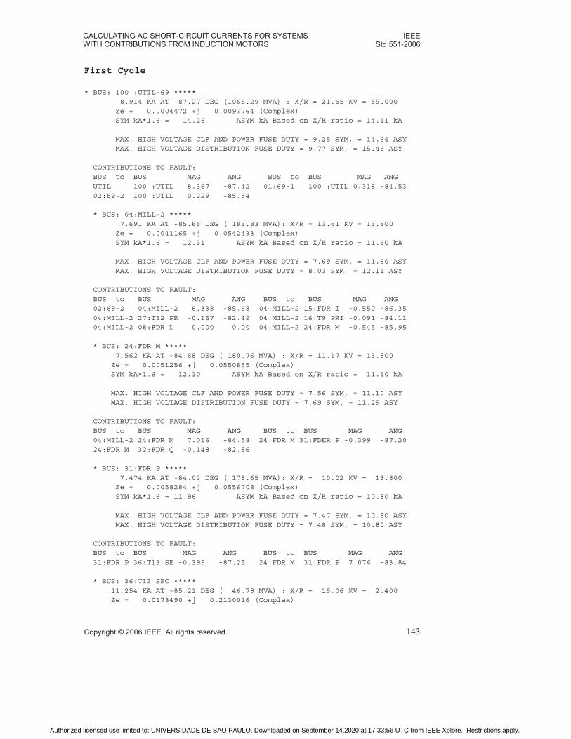
CALCULATING AC SHORT-CIRCUIT CURRENTS FOR SYSTEMS IEEEWITH CONTRIBUTIONS FROM INDUCTION MOTORS Std 551-2006
Copyright © 2006 IEEE. All rights reserved. 143
First Cycle
* BUS: 100 :UTIL-69 ***** 8.914 KA AT -87.27 DEG (1065.29 MVA) : X/R = 21.65 KV = 69.000 Ze = 0.0004472 +j 0.0093764 (Complex) SYM kA*1.6 = 14.26 ASYM kA Based on X/R ratio = 14.11 kA
MAX. HIGH VOLTAGE CLF AND POWER FUSE DUTY = 9.25 SYM, = 14.64 ASY MAX. HIGH VOLTAGE DISTRIBUTION FUSE DUTY = 9.77 SYM, = 15.46 ASY
CONTRIBUTIONS TO FAULT: BUS to BUS MAG ANG BUS to BUS MAG ANG UTIL 100 :UTIL 8.367 -87.42 01:69-1 100 :UTIL 0.318 -84.53 02:69-2 100 :UTIL 0.229 -85.54
* BUS: 04:MILL-2 ***** 7.691 KA AT -85.66 DEG ( 183.83 MVA): X/R = 13.61 KV = 13.800 Ze = 0.0041165 +j 0.0542433 (Complex) SYM kA*1.6 = 12.31 ASYM kA Based on X/R ratio = 11.60 kA
MAX. HIGH VOLTAGE CLF AND POWER FUSE DUTY = 7.69 SYM, = 11.60 ASY MAX. HIGH VOLTAGE DISTRIBUTION FUSE DUTY = 8.03 SYM, = 12.11 ASY
CONTRIBUTIONS TO FAULT: BUS to BUS MAG ANG BUS to BUS MAG ANG 02:69-2 04:MILL-2 6.338 -85.68 04:MILL-2 15:FDR I -0.550 -86.35 04:MILL-2 27:T12 PR -0.167 -82.49 04:MILL-2 16:T9 PRI -0.091 -84.11 04:MILL-2 08:FDR L 0.000 0.00 04:MILL-2 24:FDR M -0.545 -85.95
* BUS: 24:FDR M ***** 7.562 KA AT -84.68 DEG ( 180.76 MVA) : X/R = 11.17 KV = 13.800 Ze = 0.0051256 +j 0.0550855 (Complex) SYM kA*1.6 = 12.10 ASYM kA Based on X/R ratio = 11.10 kA
MAX. HIGH VOLTAGE CLF AND POWER FUSE DUTY = 7.56 SYM, = 11.10 ASY MAX. HIGH VOLTAGE DISTRIBUTION FUSE DUTY = 7.69 SYM, = 11.29 ASY
CONTRIBUTIONS TO FAULT: BUS to BUS MAG ANG BUS to BUS MAG ANG 04:MILL-2 24:FDR M 7.016 -84.58 24:FDR M 31:FDER P -0.399 -87.20 24:FDR M 32:FDR Q -0.148 -82.86
* BUS: 31:FDR P ***** 7.474 KA AT -84.02 DEG ( 178.65 MVA): X/R = 10.02 KV = 13.800 Ze = 0.0058284 +j 0.0556708 (Complex) SYM kA*1.6 = 11.96 ASYM kA Based on X/R ratio = 10.80 kA
MAX. HIGH VOLTAGE CLF AND POWER FUSE DUTY = 7.47 SYM, = 10.80 ASY MAX. HIGH VOLTAGE DISTRIBUTION FUSE DUTY = 7.48 SYM, = 10.80 ASY
CONTRIBUTIONS TO FAULT: BUS to BUS MAG ANG BUS to BUS MAG ANG 31:FDR P 36:T13 SE -0.399 -87.25 24:FDR M 31:FDR P 7.076 -83.84
* BUS: 36:T13 SEC ***** 11.254 KA AT -85.21 DEG ( 46.78 MVA) : X/R = 15.06 KV = 2.400 Ze = 0.0178490 +j 0.2130016 (Complex)
Authorized licensed use limited to: UNIVERSIDADE DE SAO PAULO. Downloaded on September 14,2020 at 17:33:56 UTC from IEEE Xplore. Restrictions apply.

IEEEStd 551-2006 CHAPTER 6
144 Copyright © 2006 IEEE. All rights reserved.
SYM kA*1.6 = 18.01 ASYM kA Based on X/R ratio = 17.18 kA
MAX. HIGH VOLTAGE CLF AND POWER FUSE DUTY = 11.26 SYM, = 17.18 ASY MAX. HIGH VOLTAGE DISTRIBUTION FUSE DUTY = 11.90 SYM, = 18.16 ASY
CONTRIBUTIONS TO FAULT: BUS to BUS MAG ANG BUS to BUS MAG ANG Med Ind 36:T13 SE 2.939 -88.08 31:FDR P 36:T13 SE 8.320 -84.20
Interrupting time
* BUS: 100 :UTIL-69 ***** 8.654 KA AT -87.37 DEG (1034.21 MVA) : X/R = 21.99 KV = 69.000 Ze = 0.0004440 +j 0.0096591 (Complex)
CONTRIBUTIONS TO FAULT: BUS to BUS MAG ANG BUS to BUS MAG ANG UTIL 100 :UTIL 8.367 -87.42 01:69-1 100 :UTIL 0.165 -85.33 02:69-2 100 :UTIL 0.121 -86.50 * BUS: 01:69-1 ***** 6.633 KA AT -81.93 DEG ( 792.74 MVA) : X/R = 7.19 KV = 69.000 Ze = 0.0017702 +j 0.0124897 (Complex)
CONTRIBUTIONS TO FAULT: BUS to BUS MAG ANG BUS to BUS MAG ANG 01:69-1 03:MILL-1 -0.166 -85.46 01:69-1 100 :UTIL -6.467 -81.84
* BUS: 04:MILL-2 ***** 6.981 KA AT -85.78 DEG ( 166.87 MVA) : X/R = 13.78 KV = 13.800 Ze = 0.0044095 +j 0.0597656 (Complex)
CONTRIBUTIONS TO FAULT: BUS to BUS MAG ANG BUS to BUS MAG ANG 02:69-2 04:MILL-2 6.321 -85.69 04:MILL-2 15:FDR I -0.393 -86.48 04:MILL-2 27:T12 PR -0.031 -85.11 04:MILL-2 16:T9 PRI 0.000 0.00 04:MILL-2 08:FDR L 0.000 0.00 04:MILL-2 24:FDR M -0.236 -86.99
* BUS: 24:FDR M ***** 6.866 KA AT -84.81 DEG ( 164.12 MVA) : X/R = 11.28 KV = 13.800 Ze = 0.0055071 +j 0.0606812 (Complex) CONTRIBUTIONS TO FAULT: BUS to BUS MAG ANG BUS to BUS MAG ANG 04:MILL-2 24:FDR M 6.630 -84.74 24:FDR M 31:FDR P -0.184 -87.68 24:FDR M 32:FDR Q -0.052 -84.81
* BUS: 31:FDR P ***** 6.790 KA AT -84.18 DEG ( 162.29 MVA) : X/R = 10.10 KV = 13.800 Ze = 0.0062527 +j 0.0612986 (Complex)
CONTRIBUTIONS TO FAULT: BUS to BUS MAG ANG BUS to BUS MAG ANG 31:FDR P 36:T13 SE -0.184 -87.70 24:FDR M 31:FDR P 6.606 -84.08
* BUS: 36:T13 SEC ***** 9.374 KA AT -84.72 DEG ( 38.97 MVA) : X/R = 12.41 KV = 2.400
Authorized licensed use limited to: UNIVERSIDADE DE SAO PAULO. Downloaded on September 14,2020 at 17:33:56 UTC from IEEE Xplore. Restrictions apply.

CALCULATING AC SHORT-CIRCUIT CURRENTS FOR SYSTEMS IEEEWITH CONTRIBUTIONS FROM INDUCTION MOTORS Std 551-2006
Copyright © 2006 IEEE. All rights reserved. 145
Ze = 0.0235982 +j 0.2555270 (Complex)
CONTRIBUTIONS TO FAULT: BUS to BUS MAG ANG BUS to BUS MAG ANG Med Ind 36:T13 SE 1.176 -88.08 31:FDR P 36:T13 SE 8.201 -84.24
6.13 Bibliography
[B1] ANSI/NEMA Std Pub. No. MG1-2003, Motors and Generators, paragraph MG1-
1.58, Dec. 1980.2, 3
[B2] Huening, Walter C. Jr., “Calculating Short-Circuit Currents with Contributions from
Induction Motors,” IEEE Transactions, IAS Vol. 1A-18, No. 2, Mar/Apr 1982.
[B3] IEC 909-1988, International Standard, Short-circuit Current Calculation in Three-
phase a.c. Systems, First edition.4
[B4] IEEE Std C37.010-1999 (Reaff 2005), IEEE Application Guide for AC High-
Voltage Circuit Breakers Rated on a Symmetrical Current Basis.5, 6
[B5] IEEE Std C37.13-1990 (Reaff 1995), IEEE Standard for Low-Voltage AC Power
Circuit Breakers Used on Enclosures.
[B6] IEEE Std C37.41-2000, IEEE Standard Design Tests for Distribution Cutouts and
Fuse Links, Secondary Fuses, Distribution Enclosed Single-Pole Air Switches, Power
Fuses, Fuse Disconnecting Switches, and Accessories.
2ANSI publications are available from the Sales Department, American National Standards Institute, 25 West43rd Street, 4th Floor, New York, NY 10036, USA (http://www.ansi.org/).3NEMA publications are available from Global Engineering Documents, 15 Inverness Way East, Englewood,Colorado 80112, USA (http://global.ihs.com/).4IEC publications are available from the Sales Department of the International Electrotechnical Commission,Case Postale 131, 3, rue de Varembé, CH-1211, Genève 20, Switzerland/Suisse (http://www.iec.ch/). IEC publi-cations are also available in the United States from the Sales Department, American National Standards Institute,11 West 42nd Street, 13th Floor, New York, NY 10036, USA.5IEEE publications are available from the Institute of Electrical and Electronics Engineers, 445 Hoes Lane, P.O.Box 1331, Piscataway, NJ 08855-1331, USA (http://standards.ieee.org/).6The IEEE standards or products referred to in this subclause are trademarks of the Institute of Electrical andElectronics Engineers, Inc.
Authorized licensed use limited to: UNIVERSIDADE DE SAO PAULO. Downloaded on September 14,2020 at 17:33:56 UTC from IEEE Xplore. Restrictions apply.

Authorized licensed use limited to: UNIVERSIDADE DE SAO PAULO. Downloaded on September 14,2020 at 17:33:56 UTC from IEEE Xplore. Restrictions apply.

Copyright © 2006 IEEE. All rights reserved. 147
Chapter 7Capacitor contributions to short-circuit currents
7.1 Introduction
Capacitor discharge currents from power factor correction capacitors or harmonic filters
have not previously been considered in the ANSI or IEC calculation procedures. The
stresses associated with capacitor discharge currents are different than typical fault
conditions due to the high-frequency components present within currents and the
extremely fast time constants of the capacitor circuits. These conditions may affect
equipment sensitive to high-frequency currents.
This section describes the nature of capacitive discharge currents during fault conditions
and the effect of capacitor currents on the total fault current. Guidelines if applicable, will
be provided for properly considering and accounting for the fault currents imposed on
equipment applied near capacitor banks. Energizing capacitors and back-to-back
switching of capacitors is not covered in this chapter.
7.2 Capacitor discharge current
A capacitor in an ac system charges and discharges in a controlled manner every half
cycle, based on the sinusoidal driving voltage and system impedances. When a fault
occurs, the system voltage is suddenly changed and the capacitor discharges at a rapid
rate, with a high discharge current. The current is greatest if the fault occurs when the
capacitor is charged to the maximum at a voltage peak. Only the impedance between the
capacitor and the fault limits the discharge current. The current will “ring down” based on
circuit resistance and reactance. The resistance provides damping and the interaction
between the system reactance and capacitor determines the frequency of the oscillating
current. The discharge current can be expressed by the Equation (7.1):
(7.1)
where
VLL = the system line-to-line voltage
L = the inductance between the capacitor bank and the fault
R = the resistance between the capacitor bank and the fault
Ipk
2
3--- VLL e
Rt L⁄– ω0t( )sin××
Z0
-----------------------------------------------------------------=
Z0LC----=
ω01
LC-----------=
Authorized licensed use limited to: UNIVERSIDADE DE SAO PAULO. Downloaded on September 14,2020 at 17:33:56 UTC from IEEE Xplore. Restrictions apply.

IEEEStd 551-2006 CHAPTER 7
148 Copyright © 2006 IEEE. All rights reserved.
In the above expression, ω0 is the natural frequency of the oscillatory circuit in radians per
second. The natural frequency is often relativity high compared to the system frequency.
The maximum peak current from the Equation (7.1) is shown in Equation (7.2) below.
(7.2)
Equation (7.2) shows that the worst-case transient fault current depends on the magnitude
of the system voltage, the inductance between the capacitor and the fault, and the
capacitance of the bank. Thus, an increase in voltage or capacitance increases the
discharge current. Since an increase in the inductance decreases the current, the distance
from the bank to the fault can be quite significant in determining the discharge current.
The magnitude of the discharge current may be negligible for equipment located farther
from the capacitor bank.
Equation (7.1) and Equation (7.2) also indicate that both the magnitude and the natural
frequency of the discharge current may be relatively high as compared to the magnitude
and frequency of the system fault currents, as demonstrated in the following example.
7.2.1 Example
The 10 Mvar capacitor bank shown in Figure 7-1 has the following capacitive reactance
and capacitance:
Xc = 19.04 Ω
C = 139.3 μF
The capacitor bank will draw |Ic| = 418.4Arms under steady-state rated conditions. The
bank is connected to the bus through 30 m of 3-1/C 500 kcmil conductors with the
following impedance:
Z’ = 0.0276 + j0.0520 Ω/300 m
Z = 0.00276 + J0.0052 Ω
so
R = 0.00276 Ω and L = 13.79 μH
This translates to a peak discharge current of 35.8 kA at a frequency of 3.631 kHz. Note
that the frequency of the discharge current is over sixty times the fundamental frequency
of the fault current. The time constant of the discharge current is the time for the current in
the series RLC circuit to reach 36 percent of its final value. In this case, the time constant
is as follows:
2Ts = L/2R = 9.99 ms
which is slightly over 1/2 of a cycle on a 60 Hz system.
Imax2
3--- VLL
CL----××=
Authorized licensed use limited to: UNIVERSIDADE DE SAO PAULO. Downloaded on September 14,2020 at 17:33:56 UTC from IEEE Xplore. Restrictions apply.

IEEECAPACITOR CONTRIBUTIONS TO SHORT-CIRCUIT CURRENTS Std 551-2006
Copyright © 2006 IEEE. All rights reserved. 149
7.3 Transient simulations
To better understand the transient response, several test systems were developed and
modeled using time-domain transient simulation software. Use of this type of software
allows complete simulation of all types of transient phenomena including the interactions
between different circuit elements to a defined disturbance. Modeling guidelines were
derived from Greenwood [B1].1
7.3.1 Standard capacitor bank
The system of Figure 7-1 was modeled to determine the effects of capacitor discharge as a
function of capacitor MVA, circuit length, and interaction with the utility source. The
example was chosen as a typical industrial supply with realistic circuit parameters similar
to field conditions.
A three-phase bolted fault was placed on the 13.8 kV bus 15 ms into the simulation while
the system was in steady-state. The faults were initiated at voltage peak in order to
maximize the current offset. The initial fault current without capacitors was calculated as
1The numbers in brackets correspond to those of the bibliography in 7.5.
Figure 7-1—One-line diagram for example case
Authorized licensed use limited to: UNIVERSIDADE DE SAO PAULO. Downloaded on September 14,2020 at 17:33:56 UTC from IEEE Xplore. Restrictions apply.

IEEEStd 551-2006 CHAPTER 7
150 Copyright © 2006 IEEE. All rights reserved.
31 340 amperes (with dc offsets included) based on the impedance looking back to the
source.
Figure 7-2 shows the results of a simulation for the case described in the previous
example. Plot 7-2(a) shows only the capacitor currents on the phase with the largest
current. The plot in Figure 7-2(b) shows the fault current contribution from the source, and
plot 7-2(c) shows the total fault current on that phase. Notice that the peak capacitor
current matches the predicted current of 35 806 A fairly closely, with a peak current of
36 253 A. The total peak fault current is 43 539 A, which occurs during the first cycle
when the current contribution from the source reaches its sinusoidal peak. Of this peak
current, the capacitor contributes roughly 25 000 A. Note that the capacitor current decays
fairly quickly.
Note that the cable model used for these calculations is a fairly simple one. The increased
resistance due to skin effect at the natural frequency is not included. The impact of cable
capacitance and coupling between phases is also neglected. Including these elements in
the model will both increase the magnitude of the initial transient and the speed the decay
of the capacitor contribution. Figure 7-3 shows fault current when the cable is modeled
first with a single coupled pi section, and second with a distributed parameter traveling
wave model (with parameters calculated at 1000 Hz). Both cases have nearly identical
maximum currents, but now the peak occurs almost immediately due to the interaction
with the cable capacitance. Note also, that the travel times for electromagnetic waves on
the 30-meter cable are very short.
Figure 7-2—Fault study with 10 Mvar capacitor separated from fault
by 30 m of cable
Authorized licensed use limited to: UNIVERSIDADE DE SAO PAULO. Downloaded on September 14,2020 at 17:33:56 UTC from IEEE Xplore. Restrictions apply.
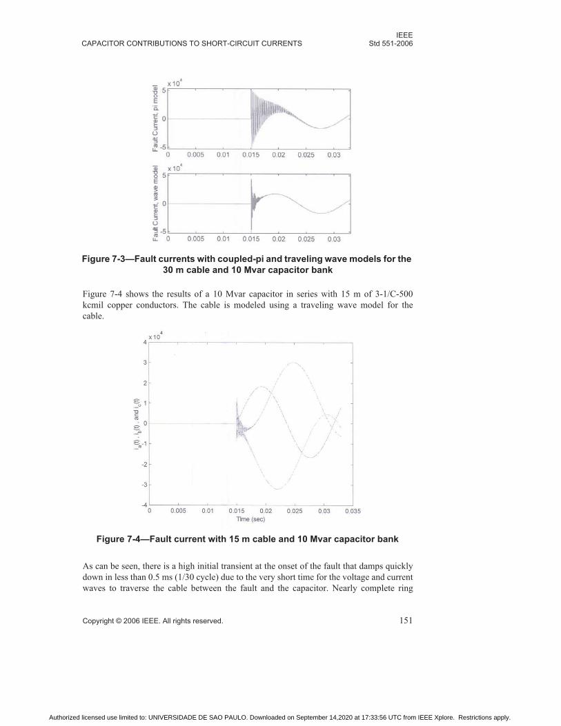
IEEECAPACITOR CONTRIBUTIONS TO SHORT-CIRCUIT CURRENTS Std 551-2006
Copyright © 2006 IEEE. All rights reserved. 151
Figure 7-4 shows the results of a 10 Mvar capacitor in series with 15 m of 3-1/C-500
kcmil copper conductors. The cable is modeled using a traveling wave model for the
cable.
As can be seen, there is a high initial transient at the onset of the fault that damps quickly
down in less than 0.5 ms (1/30 cycle) due to the very short time for the voltage and current
waves to traverse the cable between the fault and the capacitor. Nearly complete ring
Figure 7-3—Fault currents with coupled-pi and traveling wave models for the
30 m cable and 10 Mvar capacitor bank
Figure 7-4—Fault current with 15 m cable and 10 Mvar capacitor bank
Authorized licensed use limited to: UNIVERSIDADE DE SAO PAULO. Downloaded on September 14,2020 at 17:33:56 UTC from IEEE Xplore. Restrictions apply.

IEEEStd 551-2006 CHAPTER 7
152 Copyright © 2006 IEEE. All rights reserved.
down occurs in approximately 2.0 ms or 1/8 of a cycle. As can be expected, lower values
of capacitance reduce the transient and time constant.
Figure 7-5 shows the same system with 300 m of cable in order to determine the effect of
the added cable inductance on the response. Note that the peak fault currents are higher in
this case.
The initial transient is nearly ten times higher than in the 30 m cable, and takes longer to
damp down due to the longer travel times on the longer cable. Complete ring down still
occurs in approximately 2.0 ms or 1/8 of a cycle.
Standard capacitor connections show high transient discharge currents that damp quickly
before a 1/4 cycle. Low X/R ratio cables associated with industrial installations do not
increase the time constant significantly to produce extended transient times, which could
affect breaker operation.
During fault conditions, the capacitor discharge takes place in the initial 1/30–1/8 cycles,
depending on the time constant of the system. Since the breaker protective device and
contacts cannot operate in this time frame, the discharge takes place into closed contacts.
The electromagnetically induced forces of the discharge current are instantaneously
proportional to the current squared. Since the close and latch (momentary) rating of a
breaker is the maximum fundamental frequency rms fault current the breaker can
withstand, it can also be considered a measure of the forces which may be safely imposed
on the various physical members of the breaker during a rated frequency (i.e., 60 Hz) fault
condition.
To determine if the capacitor contributions could affect breaker of fuse interrupting
capability, the I2t energy in Joules was calculated for the capacitor and 60 Hz fault current
and compared. The energy was calculated for each of the cases described above. The fault
Figure 7-5—Fault current with 300 m cable separating
10 Mvar capacitor from the fault
Authorized licensed use limited to: UNIVERSIDADE DE SAO PAULO. Downloaded on September 14,2020 at 17:33:56 UTC from IEEE Xplore. Restrictions apply.
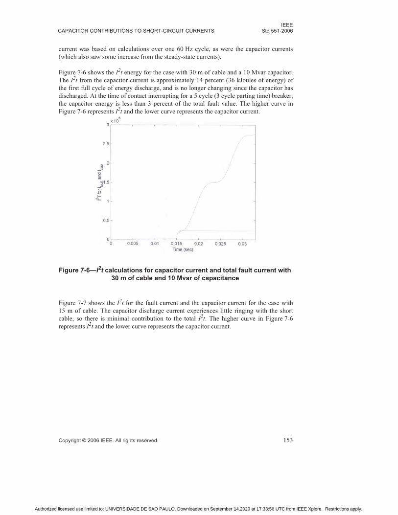
IEEECAPACITOR CONTRIBUTIONS TO SHORT-CIRCUIT CURRENTS Std 551-2006
Copyright © 2006 IEEE. All rights reserved. 153
current was based on calculations over one 60 Hz cycle, as were the capacitor currents
(which also saw some increase from the steady-state currents).
Figure 7-6 shows the I2t energy for the case with 30 m of cable and a 10 Mvar capacitor.
The I2t from the capacitor current is approximately 14 percent (36 kJoules of energy) of
the first full cycle of energy discharge, and is no longer changing since the capacitor has
discharged. At the time of contact interrupting for a 5 cycle (3 cycle parting time) breaker,
the capacitor energy is less than 3 percent of the total fault value. The higher curve in
Figure 7-6 represents I2t and the lower curve represents the capacitor current.
Figure 7-7 shows the I2t for the fault current and the capacitor current for the case with
15 m of cable. The capacitor discharge current experiences little ringing with the short
cable, so there is minimal contribution to the total I2t. The higher curve in Figure 7-6
represents I2t and the lower curve represents the capacitor current.
Figure 7-6—I2t calculations for capacitor current and total fault current with
30 m of cable and 10 Mvar of capacitance
Authorized licensed use limited to: UNIVERSIDADE DE SAO PAULO. Downloaded on September 14,2020 at 17:33:56 UTC from IEEE Xplore. Restrictions apply.

IEEEStd 551-2006 CHAPTER 7
154 Copyright © 2006 IEEE. All rights reserved.
Figure 7-8 shows approximately the same I2t ratio, as with 30 m of cable, indicating
breaker interruption should not be affected. Note that in all three cases, the I2t of the fault
current is basically the same, and only the capacitor current changes. The higher curve in
Figure 7-6 represents I2t and the lower curve represents the capacitor current.
Another concern is closing the capacitor bank into a fault when there is trapped charge on
the capacitor. The capacitor will usually be charged to either the positive or negative peak
Figure 7-7— I2t calculations for capacitor current and total fault current
with 15 m of cable and 10 Mvar of capacitance
(capacitor I2t multiplied by 100 for plotting)
Figure 7-8—I2t calculations for capacitor current and total fault current with
300 m of cable and 10 Mvar of capacitance
Authorized licensed use limited to: UNIVERSIDADE DE SAO PAULO. Downloaded on September 14,2020 at 17:33:56 UTC from IEEE Xplore. Restrictions apply.
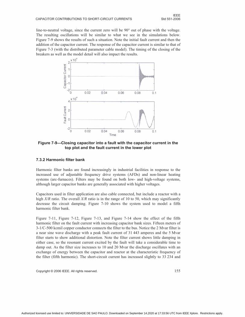
IEEECAPACITOR CONTRIBUTIONS TO SHORT-CIRCUIT CURRENTS Std 551-2006
Copyright © 2006 IEEE. All rights reserved. 155
line-to-neutral voltage, since the current zero will be 90° out of phase with the voltage.
The resulting oscillations will be similar to what we see in the simulations below.
Figure 7-9 shows the results of such a situation. Note the initial fault current and then the
addition of the capacitor current. The response of the capacitor current is similar to that of
Figure 7-3 (with the distributed parameter cable model). The timing of the closing of the
breakers as well as the model detail will also impact the results.
7.3.2 Harmonic filter bank
Harmonic filter banks are found increasingly in industrial facilities in response to the
increased use of adjustable frequency drive systems (AFDs) and non-linear heating
systems (arc-furnaces). Filters may be found on both low- and high-voltage systems,
although larger capacitor banks are generally associated with higher voltages.
Capacitors used in filter application are also cable connected, but include a reactor with a
high X/R ratio. The overall X/R ratio is in the range of 10 to 50, which may significantly
decrease the circuit damping. Figure 7-10 shows the system used to model a fifth
harmonic filter bank.
Figure 7-11, Figure 7-12, Figure 7-13, and Figure 7-14 show the effect of the fifth
harmonic filter on the fault current with increasing capacitor bank sizes. Fifteen meters of
3-1/C-500 kcmil copper conductor connects the filter to the bus. Notice the 2 Mvar filter is
a near sine wave discharge with a peak fault current of 31 443 amperes and the 5 Mvar
filter starts to show additional distortion. Note the filter current shows little damping in
either case, so the resonant current excited by the fault will take a considerable time to
damp out. As the filter size increases to 10 and 20 Mvar the discharge oscillates with an
exchange of energy between the capacitor and reactor at the characteristic frequency of
the filter (fifth harmonic). The short-circuit current has increased slightly to 33 234 and
Figure 7-9—Closing capacitor into a fault with the capacitor current in the
top plot and the fault current in the lower plot
Authorized licensed use limited to: UNIVERSIDADE DE SAO PAULO. Downloaded on September 14,2020 at 17:33:56 UTC from IEEE Xplore. Restrictions apply.

IEEEStd 551-2006 CHAPTER 7
156 Copyright © 2006 IEEE. All rights reserved.
33 285 amperes respectively. This is due to the increase in pre-fault voltage from the
capacitors, not to the capacitor discharge current.
The simulation time was extended to 3 cycles to better determine the length of the
discharge in the 10 Mvar and 20 Mvar cases. As can be seen, the oscillations last
approximately one cycle; however, the peak asymmetrical current is only 33 009 amperes,
and now appears on different phases than was the case with the capacitors instead of
filters, even if the filter current is smaller on that phase. This change results from the filter
inductance slowing down the ringing of the capacitor current, and limiting the peak
contribution from the capacitor. The 5% increase in peak asymmetrical current is due to
the increase in pre-fault voltage.
Harmonic filter connections show a decrease in transient discharge currents as compared
to a non-filtered bank. The energy exchange between the capacitor reactor combination
oscillates at the characteristic filter frequency, and the decay rate is damped as the RLC
time constant increases.
The high X/R ratio of the reactors increased the time constant significantly, however, the
added reactor impedance limited the expected high-frequency discharge to normal system
fault levels. Breaker, fuse, or switch operation should not generally be affected with this
combination. Figure 7-15 shows the I2t curves for the fault current and the filter current
for the case with a 15 meter cable and a 10 Mvar capacitor. Notice that at 33 milliseconds,
the I2t for the fault current is basically the same as it was with just a 10 Mvar capacitor in
Figure 7-7. The filter contribution continues to increase, since the filter current rings down
slowly.
In Figure 7-15, the higher curve represents the I2t of the total current while the lower curve
represents the I2t of the filter current.
Authorized licensed use limited to: UNIVERSIDADE DE SAO PAULO. Downloaded on September 14,2020 at 17:33:56 UTC from IEEE Xplore. Restrictions apply.

IEEECAPACITOR CONTRIBUTIONS TO SHORT-CIRCUIT CURRENTS Std 551-2006
Copyright © 2006 IEEE. All rights reserved. 157
Figure 7-10—One-line diagram for example case with harmonic filter bank
BUS-11
38
kV
BUS-2
13
.8 k
V
REACTOR 13
.8 k
V
UTIL-1
2500 MVA
150 (X/R)
2500 MVA
150 (X/R)
TX-1
20 MVA
138 / 13.8 kV
6%
D
YG
1
-
1
/
C
-
5
0
0
M
C
M
C
U
,
5
0
'
,
[
C
o
n
d
u
i
t
]
CAP 13
.8 k
V
5th
Harmonic
Filter Bank
Figure 7-11—Simulation results with 2 Mvar filter and 15 m of cable
Authorized licensed use limited to: UNIVERSIDADE DE SAO PAULO. Downloaded on September 14,2020 at 17:33:56 UTC from IEEE Xplore. Restrictions apply.

IEEEStd 551-2006 CHAPTER 7
158 Copyright © 2006 IEEE. All rights reserved.
Figure 7-12— Simulation results with 5 Mvar filter and 15 m of cable
Figure 7-13—Simulation results with 10 Mvar filter and 15 m of cable
Authorized licensed use limited to: UNIVERSIDADE DE SAO PAULO. Downloaded on September 14,2020 at 17:33:56 UTC from IEEE Xplore. Restrictions apply.

IEEECAPACITOR CONTRIBUTIONS TO SHORT-CIRCUIT CURRENTS Std 551-2006
Copyright © 2006 IEEE. All rights reserved. 159
Figure 7-14—Simulation results with 20 Mvar filter and 15 m of cable
Figure 7-15—I2t calculations for capacitor current and total fault
current with 1000 foot of cable and a fifth harmonic filter
with 10 Mvar of capacitance
Authorized licensed use limited to: UNIVERSIDADE DE SAO PAULO. Downloaded on September 14,2020 at 17:33:56 UTC from IEEE Xplore. Restrictions apply.

IEEEStd 551-2006 CHAPTER 7
160 Copyright © 2006 IEEE. All rights reserved.
BUS-1 138 kV
BUS-213
.8 kV
BUS-313
.8 kV
TX-1
20 MVA
138 / 13.8 kV
6%
D
YG
1-1
/C-4
/0 A
WG
CU
, 2
00
', [
Co
nd
uit
]
M-1
5000 HP
IND
16.7%
1 MVAR
13.8 kV
UTIL-1
2500 MVA
150 (X/R)
2500 MVA
150 (X/R)
7.3.3 Medium-voltage motor capacitors
The impact of medium-voltage motor capacitors was also modeled to determine the effect
of capacitor discharge along with that of the motor during a fault. Figure 7-16 shows the
system used to model the medium-voltage motor capacitor combination.
A three-phase bolted fault was placed on the 13.8 kV bus at a steady-state time of 36 ms.
The faults were initiated at voltage peak in order to maximize the current offset. The initial
fault current without capacitors was calculated as 33 852 amperes as shown in
Figure 7-17. The figure shows the fault current contribution from the source, from the
motor, and the total fault current on the same set of axes.
Figure 7-18 shows the results of a 1 Mvar capacitor in parallel with the 4-pole induction
motor. The first plot shows the capacitor current and the second shows the total fault
current. The motor and source currents are essentially unchanged, and are not shown.
Notice that the amplitude of the capacitor current is very small relative to the total fault
current.
Figure 7-16—One line diagram of example system with motor and motor
capacitor
Authorized licensed use limited to: UNIVERSIDADE DE SAO PAULO. Downloaded on September 14,2020 at 17:33:56 UTC from IEEE Xplore. Restrictions apply.

IEEECAPACITOR CONTRIBUTIONS TO SHORT-CIRCUIT CURRENTS Std 551-2006
Copyright © 2006 IEEE. All rights reserved. 161
As can be seen, there is some initial discharge below 2 ms, which is characteristic of the
standard capacitor bank results. The interaction and energy exchange with the parallel
motor capacitor combination may actually damp the discharge somewhat. Maximum fault
current was increased slightly to 33 963 amperes with capacitor addition due to the
increase in pre-fault voltage. Similar results are seen for different sized capacitor banks.
Medium-voltage motor capacitors are small enough that they show no significant increase
to the normal system fault levels.
Figure 7-17—Simulation results with capacitors disconnected
(fault current, source current and motor current)
Figure 7-18—Simulation results with capacitors connected to the system
(The capacitor current is shown in top plot and the fault current in the lower plot.)
Authorized licensed use limited to: UNIVERSIDADE DE SAO PAULO. Downloaded on September 14,2020 at 17:33:56 UTC from IEEE Xplore. Restrictions apply.

IEEEStd 551-2006 CHAPTER 7
162 Copyright © 2006 IEEE. All rights reserved.
7.3.4 Low-voltage motor capacitors
Low-voltage motor capacitors were modeled to determine the effect of capacitor
discharge with the motor during a fault. Figure 7-19 shows the system used to model the
low-voltage motor capacitor combination.
A three-phase bolted fault was placed on the 480-volt bus at a steady-state time of 36 ms.
The faults were initiated at voltage peak in order to maximize the current offset. The initial
fault current without capacitors was calculated as 33 193 amperes as shown in
Figure 7-20. The figure shows the current contribution from the source, the motor current,
and the total fault current. Figure 7-21 shows the results of a 200 kVAR capacitor added to
the switchgear bus. The first plot shows the capacitor current and the second plot shows
the total fault current. Again, the source and motor contributions are largely unchanged.
As can be seen, there is no visible discharge below. Maximum fault current was increased
slightly to 33 378 amperes with capacitor addition limited currents due to the increase in
pre-fault voltage. Low-voltage motor capacitors are small enough that they show no
significant increase to the normal system fault levels.
Authorized licensed use limited to: UNIVERSIDADE DE SAO PAULO. Downloaded on September 14,2020 at 17:33:56 UTC from IEEE Xplore. Restrictions apply.

IEEECAPACITOR CONTRIBUTIONS TO SHORT-CIRCUIT CURRENTS Std 551-2006
Copyright © 2006 IEEE. All rights reserved. 163
BUS-1 13.8
kV
SWG0.
48 k
V
MCC 0.48
kV
TX-1
1 MVA
13.8 / 0.48 kV
8%
D
YG
2-3
/C-3
50 M
CM
CU
, 2
0',
[Co
nd
uit
]
M-1
700 HP
IND
16.7%
UTIL-1
500 MVA
10 (X/R)
500 MVA
10 (X/R)
0.2 MVAR
0.48 kV
CAP 0.48
kV
1-1
/C-4
/0 A
WG
CU
, 1
0',
[Co
nd
uit
]
Figure 7-19—One line diagram of example system with low-voltage motor
capacitors
Authorized licensed use limited to: UNIVERSIDADE DE SAO PAULO. Downloaded on September 14,2020 at 17:33:56 UTC from IEEE Xplore. Restrictions apply.

IEEEStd 551-2006 CHAPTER 7
164 Copyright © 2006 IEEE. All rights reserved.
Figure 7-20—Simulation results with capacitors disconnected (fault current,
source current and motor current)
Figure 7-21—Simulation results with capacitors connected to the system
(The capacitor current is shown in top plot and the fault current in the
lower plot.)
Authorized licensed use limited to: UNIVERSIDADE DE SAO PAULO. Downloaded on September 14,2020 at 17:33:56 UTC from IEEE Xplore. Restrictions apply.

IEEECAPACITOR CONTRIBUTIONS TO SHORT-CIRCUIT CURRENTS Std 551-2006
Copyright © 2006 IEEE. All rights reserved. 165
7.4 Summary
During fault conditions, the capacitor discharge takes place in the initial 1/30–1/8 cycles,
depending on the time constant of the system. Since the breaker protective device and
contacts cannot operate in this time frame, the discharge takes place into closed contacts.
The electro-magnetically induced forces of the discharge current are instantaneously
proportional to the current squared. Since the close and latch (momentary) rating of a
breaker is the maximum fundamental frequency rms fault current the breaker can
withstand, it can also be considered a measure of the forces which may be safely imposed
on the various physical members of the breaker during a rated frequency (i.e., 60 Hz) fault
condition.
Based on the simulations shown in this chapter, capacitor discharge currents will have no
effect on breaker parting or clearing operations. Some small additional stresses may be
imposed for the closing and latching duty for very large capacitor banks. However, it
should be noted that the models developed in this chapter were sized larger than standard
design practices in order to determine any potential problems.
At this point, the standard cannot recommend that capacitors be added to system
simulations for breaker duty calculations. The existing ANSI C37 series fault calculation
methodologies remain adequate for the determination of breaker, fuse, and switch duties.
7.5 Bibliography
[B1] Greenwood, A., Electrical Transients in Power Systems, Second Edition. Wiley-
Interscience, 1991.
Authorized licensed use limited to: UNIVERSIDADE DE SAO PAULO. Downloaded on September 14,2020 at 17:33:56 UTC from IEEE Xplore. Restrictions apply.

Authorized licensed use limited to: UNIVERSIDADE DE SAO PAULO. Downloaded on September 14,2020 at 17:33:56 UTC from IEEE Xplore. Restrictions apply.

Copyright © 2006 IEEE. All rights reserved. 167
Chapter 8Static converter contributions to short-circuit currents
8.1 Introduction
This chapter examines how static power converters influence ac short-circuit currents. The
purpose of this chapter is to define when and how much a converter increases the
calculated short-circuit current for a fault nearby on the ac supply system. The chapter also
analyzes currents to dc short circuits in the converter equipment, pointing out that, under
certain circumstances, these fault currents may be larger than the normally calculated
maximum three-phase short-circuit currents. Before any equations or calculations are
presented, some definitions of converter types and their possible fault conditions are
given.
8.2 Definitions of converter types
A power converter links two systems with different frequencies or to a dc voltage.
A static power converter is a converter that employs static switching devices such as
diodes, SCRs, metallic controlled rectifiers, transistors, electron tubes, or magnetic
amplifiers. All these types of switching devices will be called valves in this chapter. All
valves may be considered in two groups: without or with a grid control system; the
corresponding converters are referred to as non-controlled or controlled. The difference
between the two is that non-controlled converter’s valves conduct at moments when the
valve voltage becomes positive and controlled converter’s valves conduct at moments
when the valve voltage is positive and a grid-control pulse is supplied. The angle between
the moment when the valve voltage becomes positive and the moment the grid-control
pulse is supplied is called the firing angle (0 ≤ α ≤ 180º).
The damage of a short circuit in a controlled converter system can be significantly limited
by the grid-control protection system. A grid-control protection system enables the grid
firing circuit to detect abnormal conditions and stop sending grid pulses. The current flow
to a converter short circuit is limited to one cycle by the normal action of the grid
protection system.
There are four main types of converters:
1) Rectifier—A converter that converts alternating current/voltage to direct current/
voltage (ac to dc).
2) Inverter—A converter that converts direct current/voltage to alternating current/
voltage (dc to ac).
3) Cycloconverter—A converter that converts alternating current of one frequency to
alternating current of another frequency (ac to ac).
4) Chopper —A converter that converts dc to dc of another voltage.
Authorized licensed use limited to: UNIVERSIDADE DE SAO PAULO. Downloaded on September 14,2020 at 17:33:56 UTC from IEEE Xplore. Restrictions apply.

IEEEStd 551-2006 CHAPTER 8
168 Copyright © 2006 IEEE. All rights reserved.
In this chapter, in addition to dc contributions through inverting converters to ac short
circuits, dc short circuits in rectifiers and inverters and their current from the ac system are
analyzed and calculated.
8.3 Converter circuits and their equivalent parameters
There are many types of converter circuits; however, two are the most common and they
are analyzed in this chapter. These two circuits are the three-phase half-wave circuit
(Figure 8-1a) and the three-phase full-wave circuit also known as the three-phase bridge
(Figure 8-1b). These circuits are used in all types of converters such as rectifiers, inverters,
and cycloconverters.
The ac equivalent circuits of the converters are shown in Figure 8-2a and Figure 8-2b
where the ac system and transformer are changed to the symmetrical three-phase voltages
labeled e1, e2, and e3, and the current in each phase is limited by system and transformer
inductive reactance Xγ and resistance Rγ. The formulae for the Xγ calculations are as
follows:
(8.1)
(8.2)
(8.3)
(8.4)
where
Xs is the equivalent inductive system reactance
V1 is the effective value of the system line-to-line voltage
Ssc is the three-phase short-circuit power (available short-circuit MVA) of the
ac system at the transformer primary terminals
Xt and Xt% is the inductive reactance of the transformer in ohms and in percentage
V2 is the effective value of the line-to-line voltage of the transformer
secondary winding under no load conditions
S is the rated MVA power of the transformer
Em is the peak amplitude of the transformer secondary winding phase voltage.
(See Figure 8-1a and Figure 8-1b.)
The equation for the Rγ calculation is similar to Equation (8.1), Equation (8.2), and
Equation (8.3) with each X value changed to the corresponding R value.
Xγ Xt V2 V1⁄( )2 X× S+=
XS V1
2 SSC⁄=
Xt Xt% 100⁄( ) V2
2 S⁄×=
V2
3
2-------Em=
Authorized licensed use limited to: UNIVERSIDADE DE SAO PAULO. Downloaded on September 14,2020 at 17:33:56 UTC from IEEE Xplore. Restrictions apply.

IEEESTATIC CONVERTER CONTRIBUTIONS TO SHORT-CIRCUIT CURRENTS Std 551-2006
Copyright © 2006 IEEE. All rights reserved. 169
Figure 8-1—Converter circuits and their connections
(a) Half-wave converter
(b) Full-wave converter
Figure 8-2—AC equivalent circuit of converters
(a) Half-wave converter
(b) Full-wave converter
Authorized licensed use limited to: UNIVERSIDADE DE SAO PAULO. Downloaded on September 14,2020 at 17:33:56 UTC from IEEE Xplore. Restrictions apply.

IEEEStd 551-2006 CHAPTER 8
170 Copyright © 2006 IEEE. All rights reserved.
8.4 Short-circuit current contribution from the dc system to an ac
short circuit
This analysis considers an ac short circuit with a dc current contribution from a dc
machine that is SCR-fed from the ac system.
The dc system contributes current to an ac short circuit only when the converter operates
as an inverter. Only then can the dc system feed energy to the ac system. Because non-
regenerative motor drives cannot operate in inverter mode (as viewed by the ac system),
they are not considered for short-circuit calculations. The circuit for analysis is developed
from Figure 8-1 by changing load resistance R to a dc source Ed with internal resistance
Rd, as shown in Figure 8-3. The inverter circuit operates with SCRs; only SCR converters
are analyzed here.
The dc sources of voltage Ed that are of principal interest in this text are dc machines,
normally motors but operating transiently as generators while their converters are
inverting. Other possible sources, some having different characteristics for Ed, include
batteries (perhaps in Uninterruptible Power Supplies), photo-voltaic arrays, and inverters
(perhaps of dc transmission lines); these are only of passing interest in industrial or
commercial building power systems.
Figure 8-3—Equivalent diagram with inverter source and possible points of
short circuits on ac side
1. High-voltage primary of supply transformer
2. High-voltage primary of converter transformer
3. Low-voltage secondary of converter transformer
Authorized licensed use limited to: UNIVERSIDADE DE SAO PAULO. Downloaded on September 14,2020 at 17:33:56 UTC from IEEE Xplore. Restrictions apply.

IEEESTATIC CONVERTER CONTRIBUTIONS TO SHORT-CIRCUIT CURRENTS Std 551-2006
Copyright © 2006 IEEE. All rights reserved. 171
Only dc machine sources are analyzed in this chapter. Under normal operating conditions,
the voltage Ed and the voltage ud on the converter terminals, produced by the ac voltage
E~, are practically equal, and rated currents I~ and Id flow in the ac and dc systems, as in
Figure 8-4. When the ac short circuit occurs, short-circuit currents flow to it from the ac
system and may flow also from the dc system if the converter is inverting. The largest
short-circuit currents flow when the voltage E~ falls to zero. This occurs with a three-
phase symmetrical ac short circuit at any one of the points 1, 2, or 3 in Figure 8-3 between
the ac system and the converter. In this case, the ac and dc fault currents are independent
of each other, can be determined separately, and add together only at the fault point.
The equivalent diagrams for the half wave and full wave converters with an ac short
circuit are shown in Figure 8-5, where the symbols are as follows:
R1, X1 = total resistance and reactance between the converter and the point of ac
short circuit
BV = the bypass valve
Rd, Xd = the total resistance and reactance of the dc elements
Figure 8-4—Simplest equivalent diagram of ac and dc systems
Authorized licensed use limited to: UNIVERSIDADE DE SAO PAULO. Downloaded on September 14,2020 at 17:33:56 UTC from IEEE Xplore. Restrictions apply.

IEEEStd 551-2006 CHAPTER 8
172 Copyright © 2006 IEEE. All rights reserved.
If the grid-control protection system operates, the BV is fired immediately after the ac
short circuit occurs. This diverts the dc contribution to the ac short circuit (the dc system
current flows through the BV) and the dc system contributes to the short-circuit current
only for the short time (less than one cycle) before the BV fires.
If the grid-control protection system does not operate, the grid pulses are not supplied to
the valve grids and the valves that are conducting when the ac short circuit occurs
continue to conduct current from the dc motor acting as a source to the ac short circuit. For
conservatism, the initial analysis assumes the dc machine has electrical armature
transients that are faster than mechanical (slowdown) and electrical field transients,
permitting the assumption that back emf Ed is essentially constant. For this assumption,
the equivalent diagrams for the fault of the half-wave and full-wave converters during
non-commutating and commutating intervals are shown in Figure 8-6 and Figure 8-7. The
resultant circuits are linear RL circuits with source Ed. The standard equation for such
circuits is shown in Equation (8.5).
(8.5)
The maximum value of current, at t = ∞, is equal to:
(8.6)
where
Ed is a constant
τdc = RΣ/LΣ is the time constant in seconds of the dc short-circuit current
Figure 8-5—Equivalent diagram of half-wave (a) and full-wave
(b) converters with the short-circuit on the ac side
i IΣ 1 ε t τ⁄––( )× i 0( ) ε t τdc⁄–×+=
IΣ Ed rΣ⁄=
Authorized licensed use limited to: UNIVERSIDADE DE SAO PAULO. Downloaded on September 14,2020 at 17:33:56 UTC from IEEE Xplore. Restrictions apply.

IEEESTATIC CONVERTER CONTRIBUTIONS TO SHORT-CIRCUIT CURRENTS Std 551-2006
Copyright © 2006 IEEE. All rights reserved. 173
RΣ and LΣ are the total resistance and inductance of the dc circuit to the ac short-
circuit point
i(0) is the initial dc circuit current
The magnitudes of RΣ for different converters and short-circuit current paths are shown in
Table 8-1, refer to Figure 8-6 and Figure 8-7. Values of LΣ are obtained from Table 8-1 by
changing each resistance R to the corresponding value of inductance L. If X is known
instead of L, divide it by 2πf.
Table 8-1—Magnitudes of RΣ
Current paths Half wave Full wave
One (non-commutating interval) R1 + Rd 2 × R1 + Rd
Two (commutating interval) (R1/2) + Rd (3 × R1/2) + Rd
Figure 8-6—Equivalent diagram of half-wave (a) and full-wave (b) converters
for the dc contribution to an ac short-circuit during a
non-commutation interval
Authorized licensed use limited to: UNIVERSIDADE DE SAO PAULO. Downloaded on September 14,2020 at 17:33:56 UTC from IEEE Xplore. Restrictions apply.

IEEEStd 551-2006 CHAPTER 8
174 Copyright © 2006 IEEE. All rights reserved.
For dc machines with comparably fast mechanical and electrical transients, the dc source
may be represented as a capacitor with an initial voltage Ed. The equivalent circuit is an
RLC circuit, Figure 8-8(a). The equivalent capacitance C represents the dc machine
slowdown including the influences of inertia, mechanical load and friction on speed decay
and of field current decay on voltage. The current of the equivalent circuit is a damped
sinusoid, Figure 8-8(b), with a highest first peak and initial rate of rise both lower than for
the RL circuit. A more complete analysis covering this is not included here because it is
conservative to analyze all cases using the RL circuit.
The following summarizes the preceding analysis of the contributions of dc machines to
ac short-circuit currents:
Figure 8-7—Equivalent diagram of half-wave (a) and full-wave
(b) converters for the dc contribution to an ac short-circuit
during a commutation interval
Figure 8-8—Equivalent diagram of oscillatory circuit (a) and
short-circuit current (b)
Authorized licensed use limited to: UNIVERSIDADE DE SAO PAULO. Downloaded on September 14,2020 at 17:33:56 UTC from IEEE Xplore. Restrictions apply.

IEEESTATIC CONVERTER CONTRIBUTIONS TO SHORT-CIRCUIT CURRENTS Std 551-2006
Copyright © 2006 IEEE. All rights reserved. 175
a) If the grid-control protection system operates to fire a bypass valve, the dc system
contributes to the short-circuit current only for the short time (less than one cycle)
before the BV fires.
b) If the grid-control protection system does not operate, the contribution of dc short-
circuit current depends on the character of the source. IΣ = Ed/RΣ final maximum
dc current applies for a dc machine with electrical armature transients faster than
mechanical and dc field transients so that the voltage source Ed is constant and the
equivalent circuit is an RL circuit.
Note that the dc short-circuit current contributed in the real system will be smaller than
calculated here not only due to dc machine slowdown but also due to the damping of dc
currents in the converter transformers. Other effects of high magnitude dc currents that are
difficult to evaluate quantitatively also tend to limit the magnitude or duration of the dc
contribution. These include tripping of dc circuit breakers, blowing of SCR valve fuses,
and possibly dc machine commutator flashovers. Since the current flow to a converter
short circuit is limited to one cycle by the normal action of the grid protection system, it is
necessary to calculate only the dc current contribution that adds to the ac first cycle peak
and rms short-circuit current. The dc short-circuit current contribution may also have a
strong influence on the after-fault system recovery, because it tends to saturate the
converter transformer core. When the short circuit is cleared and the ac primary bus is
reenergized, there may be a very large inrush of current to the transformer.
The highest peak current of the ac system short circuit, Iacpeak, before it is increased by the
dc current contribution through the inverting converter from the dc machine, occurs
during the first cycle of the most offset phase current. It was noted in Chapter 2 that peak
ac depends on the symmetrical component of the ac current, Isym, peak, and the fault point
X/R ratio to be approximately:
(8.7)
where τ = 0.49 – 0.1ε–(X/R)/3
The most offset ac system current reaches this highest peak in less than one half cycle (at
system frequency) after the short circuit occurs. To use a conservative simplification, the
transiently increasing dc current fault contribution, ic, that is added to the first cycle peak
ac current, is calculated at the half cycle time (0.00833 seconds at 60 Hz or 0.01 seconds at
50 Hz).
The magnitude of the dc current fault contribution ic at a time equal to one-half cycle at
system frequency is shown in Equation (8.8) [from Equation (8.5)]:
(8.8)
To summarize, the dc contribution of a controlled or non-controlled inverting converter to
an ac system short-circuit current is estimated by adding ic at one-half cycle based on
system frequency to the highest first cycle ac peak current.
Iac, peak Isym, peak 1 ε 2πτ X R⁄( )–+[ ]=
ic Id Id i 0( )–( )επ XΣ RΣ⁄( )–
–=
Authorized licensed use limited to: UNIVERSIDADE DE SAO PAULO. Downloaded on September 14,2020 at 17:33:56 UTC from IEEE Xplore. Restrictions apply.

IEEEStd 551-2006 CHAPTER 8
176 Copyright © 2006 IEEE. All rights reserved.
The “source plus impedance” circuit component that represents the dc machine
contributing through an inverting converter in the equivalent circuit for an ac short-circuit
calculation, as recommended by IEC 60909-0:2001 [B7]1, is the same as that of an
induction motor. This circuit component has an impedance corresponding to an
“equivalent locked rotor current” of 3.0 per-unit, (X" = 33%) based on the ac three-phase
apparent power input of the converter transformer (or of the converter if there is no
transformer) at rated dc machine load and an equivalent X/R ratio of 10. The Grotstollen
investigation [B3] is essentially in agreement with this equivalent representation.
8.5 Analysis of converter dc faults
There are two types of converter short circuits that cause the flow of large currents in ac
supply systems: one is a short circuit between the dc terminals of a converter and the other
is a short circuit of one of the converter valves also called an “arc-back.”
The short circuit effects can be very severe if the grid-control protection system does not
operate and grid pulses continue to be supplied under fault conditions. The most severe
faults occur in diode converters where there is no grid-control protection system.
The short circuits analyzed in this chapter are as follows:
1) A short-circuit between the dc terminals of a converter with a grid-control
protection system.
2) A short-circuit between the dc terminals of a converter without a grid-control
protection system.
3) An arc-back with a grid-control protection system.
4) An arc-back without a grid-control protection system.
Short circuits are analyzed in the above sequence for the half- and full-wave converters,
shown in Figure 8-1 and Figure 8-2. All calculations are carried out for the no-load initial
condition when the fault current is maximum.
The full analysis of a converter dc short circuit (not within the scope of this text) includes
the definition and solution of sets of linear differential equations and/or difference τs for
the various types of short-circuit currents. The fault currents depend on the resistance and
reactance of the ac system and the moment when the short circuit occurs.
To simplify the analysis, the following assumptions are made:
a) The short-circuit current path for each case is as shown on the figures illustrating
the circuit diagram for the case.
b) The short-circuit currents are calculated neglecting circuit resistance. These cur-
rents can be modified to account for the damping due to resistance by
Equation (8.7) using Xγ/Rγ.
c) The term Im = Em/Xγ is used in all equations.
1The numbers in brackets correspond to those of the bibliography in 8.10.
Authorized licensed use limited to: UNIVERSIDADE DE SAO PAULO. Downloaded on September 14,2020 at 17:33:56 UTC from IEEE Xplore. Restrictions apply.

IEEESTATIC CONVERTER CONTRIBUTIONS TO SHORT-CIRCUIT CURRENTS Std 551-2006
Copyright © 2006 IEEE. All rights reserved. 177
The parameters Em, Xγ, and Rγ are defined in 8.3. Im is the peak of the symmetrical phase
current to a three-phase ac short circuit at the ac input terminals of the converter.
A dc short circuit inside or at the dc output terminals of a converter may have currents
similar magnitude to those of a three-phase ac short circuit at the ac input terminals, but
the peak short-circuit currents can be larger than the 2Im calculated for the ac short circuit.
8.6 Short circuit between the converter dc terminals
The first fault considered is a short circuit between the dc terminals of the half-wave
converter shown in Figure 8-9. This short circuits every ac phase. If the grid-control
protection system operates, the fault current flows only in the one phase whose voltage is
the most positive at the moment when the fault occurs. The other two phases have no fault
currents because the grid-control protection system feeds no grid pulses, as in line (2),
Figure 8-10. The equivalent three-phase voltages of line (1) of Figure 8-10 are shown in
Equation (8.9):
(8.9)
where Em is the maximum amplitude of the phase voltage.
The short-circuit current has a maximum peak when the fault occurs at θ = α firing angle,
and the grid impulse is supplied to phase 1, see location (2), Figure 8-10. The equation for
the current from the ac system to the dc short circuit is shown in Equation (8.10):
(8.10)
where isc = 0 at θ = α, locations (3) and (4), Figure 8-10, and Im = Em/Xγ is the peak of the
symmetrical ac current to a three-phase bolted short circuit at the converter input
terminals.
The non-damped peak of the ac current to the dc short circuit is shown in Equation (8.11):
(8.11)
The actual peak magnitude of the decaying ac current to the dc short circuit accounting for
resistive damping, Rγ, is obtained using the dependent multiplying factor, MFdcfault,
derived from Equation (8-7). Im replaces Isym, peak or √2Isym and MFdcfault = (first cycle
asymmetrical current)/(peak of ac symmetrical current).
(8.12)
where
e1 Em θ 30°+( )sin×= e2 Em θ 90– °( )sin×= e3 Em θ 150°+( )sin×=
isc Im α 30°+( )cos( α θ 30°+ +( ) )cos–=
ipsc Im 1( α 30°+( ) )cos+=
MFdefault Im 1 e2πτ Xϒ Rϒ⁄( )–
+[ ]=
τ 0.49 0.1e2πτ Xϒ Rϒ⁄( ) 3⁄–
–=
Authorized licensed use limited to: UNIVERSIDADE DE SAO PAULO. Downloaded on September 14,2020 at 17:33:56 UTC from IEEE Xplore. Restrictions apply.

IEEEStd 551-2006 CHAPTER 8
178 Copyright © 2006 IEEE. All rights reserved.
If the grid-control protection system does not operate, the analysis is similar to the above
except the short circuit currents flow in all three ac phases and repeat every cycle as
shown in Figure 8-11.
In the case of the diode converter there is no grid-protection system. The diodes begin to
conduct when their anode voltages become positive. The equation for the current from the
ac system to the dc short circuit is shown in Equation (8.13):
(8.13)
and its non-damped peak value is shown in Equation (8.14):
(8.14)
isc Im 1 θcos–( )=
Ipsc 2Im=
Figure 8-9—DC short-circuit between half-wave converter terminals
Authorized licensed use limited to: UNIVERSIDADE DE SAO PAULO. Downloaded on September 14,2020 at 17:33:56 UTC from IEEE Xplore. Restrictions apply.

IEEESTATIC CONVERTER CONTRIBUTIONS TO SHORT-CIRCUIT CURRENTS Std 551-2006
Copyright © 2006 IEEE. All rights reserved. 179
Figure 8-10—DC terminal short-circuit in a half-wave SCR converter
(grid protection system operates)
1. Three-phase voltage system
2. Grid impulse
3. Fault loop
4. Fault current in phase 1 only
Authorized licensed use limited to: UNIVERSIDADE DE SAO PAULO. Downloaded on September 14,2020 at 17:33:56 UTC from IEEE Xplore. Restrictions apply.

IEEEStd 551-2006 CHAPTER 8
180 Copyright © 2006 IEEE. All rights reserved.
Figure 8-11—DC terminal short-circuit in a half-wave SCR converter
(grid protection system does not operate)
1. Three-phase voltage system
2. Grid impulse
3,4,5. Fault current in phase 1, 2, and 3.
Authorized licensed use limited to: UNIVERSIDADE DE SAO PAULO. Downloaded on September 14,2020 at 17:33:56 UTC from IEEE Xplore. Restrictions apply.

IEEESTATIC CONVERTER CONTRIBUTIONS TO SHORT-CIRCUIT CURRENTS Std 551-2006
Copyright © 2006 IEEE. All rights reserved. 181
The short-circuit currents flow in all three phases and repeat every cycle, as shown in
Figure 8-12.
The actual peak magnitude of the decaying ac current to the dc short circuit accounting for
resistive damping is obtained using Equation (8.12).
Consider next a short circuit between the dc terminals of the full-wave converter shown in
Figure 8-13. The numbers of the valves in Figure 8-13 correspond to the valve firing
sequence. If the grid-control protection system operates, there are two possible short-
circuit current paths: one is with two valves conducting and the other is with three valves
conducting at the moment of short circuit initiation. Both have the same maximum value
Figure 8-12—DC terminal short-circuit in the diode half-wave converter
1. Three-phase voltage system
2,3,4. Fault current in phase 1, 2, and 3
Authorized licensed use limited to: UNIVERSIDADE DE SAO PAULO. Downloaded on September 14,2020 at 17:33:56 UTC from IEEE Xplore. Restrictions apply.

IEEEStd 551-2006 CHAPTER 8
182 Copyright © 2006 IEEE. All rights reserved.
of current and therefore only the circuit with two firing valves will be analyzed, see
Figure 8-14.
Figure 8-13—DC terminal short-circuit in a full-wave converter terminals
Authorized licensed use limited to: UNIVERSIDADE DE SAO PAULO. Downloaded on September 14,2020 at 17:33:56 UTC from IEEE Xplore. Restrictions apply.

IEEESTATIC CONVERTER CONTRIBUTIONS TO SHORT-CIRCUIT CURRENTS Std 551-2006
Copyright © 2006 IEEE. All rights reserved. 183
Assume the fault is initiated at the moment θ = α and two valves 1 and 4 begin to conduct.
The corresponding current from the ac system to this two-phase dc short circuit is shown
in Equation (8.15):
(8.15)
and it non-damped peak value at α = 0 is shown in Equation (8.16):
(8.16)
Figure 8-14—DC terminal short-circuit in a full-wave SCR converter
(grid protection system operates)
1. Three-phase voltage system
2. Grid impulse
3. Fault loop
4. Fault current
isc i1sc i4sc
3
2-------��
�� Im θ 30°–( )sin α 30°–( )sin–( )××= = =
Ipsc
3 3×4
----------------Im=
Authorized licensed use limited to: UNIVERSIDADE DE SAO PAULO. Downloaded on September 14,2020 at 17:33:56 UTC from IEEE Xplore. Restrictions apply.

IEEEStd 551-2006 CHAPTER 8
184 Copyright © 2006 IEEE. All rights reserved.
The actual peak magnitude of the decaying ac current to the dc short circuit accounting for
resistive damping is obtained using Equation (8.7).
If the grid-control protection system does not operate, the short-circuit current during the
first 60º is the same as when the grid-control protection system operates. At the moment
θ = 60º + α, lines (1) – (4), Figure 8.15; however, valve 2 begins to conduct.
With three valves (4, 1, and 2) conducting, there is a three-phase dc short circuit in the
converter. Taking into account the initial conditions, the three currents from the ac system
to the dc short circuit are shown in Equation (8.17), Equation (8.18), and Equation (8.19):
(8.17)
(8.18)
(8.19)
The non-damped peak values of the short circuit currents at α = 0 are shown in
Equation (8.20) and Equation (8.21):
(8.20)
(8.21)
In this case, the fault current peaks are smaller than the maximum peak for a three-phase
short circuit. This is similar to the short circuited half-wave controlled converter.
I1sc Im 1( 3
2-------+ α αsin )–cos×=
I2sc Im 1 α α 30°+( ) )cos×cos+(=
i3sc∗ Im 1
1
2--- αsin )×+�
�=
I1psc I2psc 1( 3
2-------�
� Im+= =
I3pse Im=
Authorized licensed use limited to: UNIVERSIDADE DE SAO PAULO. Downloaded on September 14,2020 at 17:33:56 UTC from IEEE Xplore. Restrictions apply.
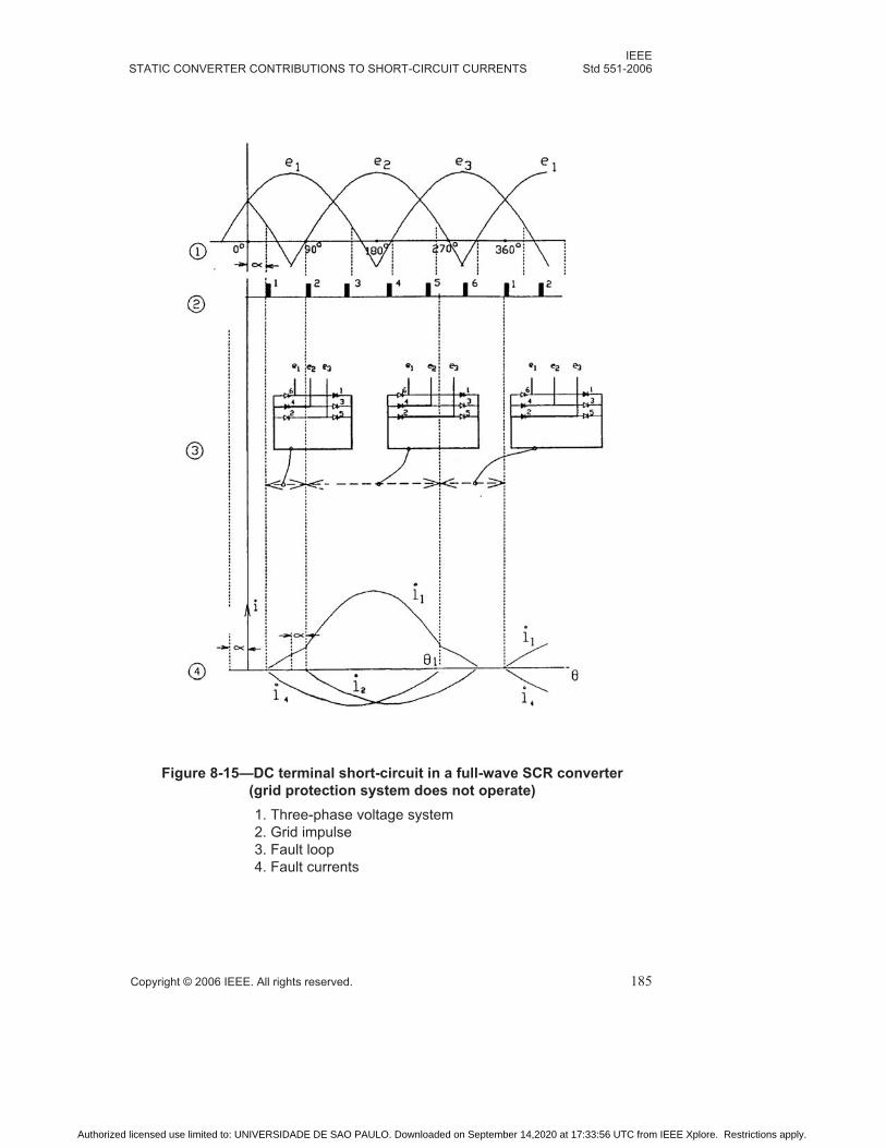
IEEESTATIC CONVERTER CONTRIBUTIONS TO SHORT-CIRCUIT CURRENTS Std 551-2006
Copyright © 2006 IEEE. All rights reserved. 185
Figure 8-15—DC terminal short-circuit in a full-wave SCR converter
(grid protection system does not operate)
1. Three-phase voltage system
2. Grid impulse
3. Fault loop
4. Fault currents
Authorized licensed use limited to: UNIVERSIDADE DE SAO PAULO. Downloaded on September 14,2020 at 17:33:56 UTC from IEEE Xplore. Restrictions apply.

IEEEStd 551-2006 CHAPTER 8
186 Copyright © 2006 IEEE. All rights reserved.
In the case of the diode converter where there is no grid-control, the fault will always be a
three-phase dc short circuit because there will always be three diodes under positive
voltage at the moment when the fault occurs (see Figure 8-16). The short-circuit current
and its non-damped peak magnitude are shown in Equation (8.22) and Equation (8.23):
(8.22)
(8.23)
i1sc Im 1 αcos+( )=
i1psc 2Im= at α 0=
Figure 8-16—DC terminal short-circuit in the diode full-wave converter1. Three-phase voltage system
2. Fault loops
3. Fault current
Authorized licensed use limited to: UNIVERSIDADE DE SAO PAULO. Downloaded on September 14,2020 at 17:33:56 UTC from IEEE Xplore. Restrictions apply.

IEEESTATIC CONVERTER CONTRIBUTIONS TO SHORT-CIRCUIT CURRENTS Std 551-2006
Copyright © 2006 IEEE. All rights reserved. 187
8.7 Arc-back short circuits
In an arc-back, one of the valves loses its semiconducting properties, forms a physical
connection, and continues to conduct. Analysis of converter design and operating
experience shows that arc-back or failure of semiconducting rectifiers are the most
common faults of converter systems. The calculation of arc-back currents is, therefore,
one of the important concerns in the theory and application of converter systems.
The greatest arc-back current occurs in a converter at no-load. In this state, both the three-
phase half-wave and full-wave converters can be reduced to the circuit diagram of the
half-wave converter shown in Figure 8-17.
If the grid-control protection system operates, the arc-back failure valve and the normal
operating valve together form a two-phase dc short-circuit loop, Figure 8-18.
The current from the ac system to this dc short-circuit loop is shown in Equation (8.24):
(8.24)
and the non-damped peak values of the current to the dc short circuit are shown in
Equation (8.25) and Equation (8.26):
(8.25)
(8.26)
isc
3
2------- Im α θcos–cos( )××=
ipsc
3
2------- Im 1( α ),cos+ α 0≠××=
Ipsc 3Im, α 0==
Figure 8-17—Three-phase converter circuit (no-load condition)
with arc-back on phase 3
Authorized licensed use limited to: UNIVERSIDADE DE SAO PAULO. Downloaded on September 14,2020 at 17:33:56 UTC from IEEE Xplore. Restrictions apply.

IEEEStd 551-2006 CHAPTER 8
188 Copyright © 2006 IEEE. All rights reserved.
Since the grid pulses are stopped after the fault occurs, the duration of the short-circuit
current is usually not more than one period. However, industrial experience with power
converters has shown that sometimes a large arc-back short-circuit current causes another
arc-back in the normally operating valve and the failure becomes an ac power frequency
two-phase short circuit that is disconnected by a circuit breaker. This is known as a
sequential arc-back.
If the grid-control protection system does not operate, the arc-back short-circuit current
during the first 120º coincides with the arc-back current described above. After the initial
120º interval, a grid pulse is applied to the phase 2 valve and a three-phase short-circuit
condition lasts for the duration of the first 360º period, see Figure 8-19. The current in the
second 360º period will be larger than in the first since the initial fault current does not
Figure 8-18—Arc-back short-circuit with operation of grid protection
1. Three-phase voltage system
2. Fault loop
3. Fault current
Authorized licensed use limited to: UNIVERSIDADE DE SAO PAULO. Downloaded on September 14,2020 at 17:33:56 UTC from IEEE Xplore. Restrictions apply.

IEEESTATIC CONVERTER CONTRIBUTIONS TO SHORT-CIRCUIT CURRENTS Std 551-2006
Copyright © 2006 IEEE. All rights reserved. 189
equal zero at the beginning of the second cycle. Later on, the fault current reaches a steady
state having the maximum amplitude. The conditions of current continuity for real
converters are dependent on α, R, and ΔU, where ΔU is the voltage drop across the valve
in the conducting mode. The fields of arc-back continuous current are shown in
Figure 8-20, where Δu = ΔU/Em. The maximum current values are also dependent on α, R,
and ΔU; if two of these parameters are known, Figure 8-20 determines the third.
Neglecting R and Δu, the τ for the current from the ac system to the arc-back dc short
circuit is written in the simplified form shown in Equation (8.27):
(8.27)
where n is the number of the period from the start of the fault.
The non-damped peak current, with α = 0, is as shown in Equation (8.28):
(Above the three-phase maximum peak) (8.28)
In the case of the diode converter, the arc-back process qualitatively is the same as
described above for the case where the grid-control protection does not operate. However,
the diodes start to conduct when their anode voltage becomes positive (at 0 = 30º, 90º, and
210º; see Figure 8-16), therefore for the calculations of the currents amplitudes it is
necessary to take α – 30º. The arc-back continuous current is found using Figure 8-20.
The maximum current occurs for R = 0, Δu = 0 and α = –30º. The dc short circuit is as
shown in Equation (8.29):
(8.29)
The non-damped peak of the current to the diode converter arc-back is as shown in
Equation (8.30):
(Above the three-phase maximum peak) (8.30)
isc Im 1( 2 α 30°+( ) ) 11
4---� �� �
n
–� �� �×cos×+=
Ipsc 2.73Im=
isc 3Im 11
4---� �� �
n
–� �� �=
Ipsc 3Im=
Authorized licensed use limited to: UNIVERSIDADE DE SAO PAULO. Downloaded on September 14,2020 at 17:33:56 UTC from IEEE Xplore. Restrictions apply.

IEEEStd 551-2006 CHAPTER 8
190 Copyright © 2006 IEEE. All rights reserved.
Figure 8-19—Arc-back short-circuit without operation of grid protection
1. Three-phase voltage system
2. Fault loops
3. Fault current
Authorized licensed use limited to: UNIVERSIDADE DE SAO PAULO. Downloaded on September 14,2020 at 17:33:56 UTC from IEEE Xplore. Restrictions apply.

IEEESTATIC CONVERTER CONTRIBUTIONS TO SHORT-CIRCUIT CURRENTS Std 551-2006
Copyright © 2006 IEEE. All rights reserved. 191
8.8 Examples
The following are examples of calculations for the “typical” converter circuit of
Figure 8-21. Data for the circuit is given below:
System voltage V1 = 13.8 kV, 60 Hz Available short circuit Ssc = 500 MVA
Rated transformer power S = 6.45 MVA
Primary voltage V1 = 13.8 kV
Secondary voltage V2 = 665 V
Transformer impedance Zt = 8.5%
Transformer X/R ratio Xt/Rt = 12
Converter filter resistance R = 0.0188 ohms
Converter filter inductance L = 1.28 × 10⁻³ H
DC motor drive power rating 6000 HP
DC motor rated voltage Ud = 700 V
DC motor rated current Id = 4830 A
DC motor rated speed 40/100 rev/m
DC motor inductance Lm = 0.852 × 10⁻³ H
DC motor resistance Rm = 0.01248 ohms at To
Normal operating temperature To
Figure 8-20—Fields of arc-back continuous currents, inter-relation of
Δu, R/X, and α
Authorized licensed use limited to: UNIVERSIDADE DE SAO PAULO. Downloaded on September 14,2020 at 17:33:56 UTC from IEEE Xplore. Restrictions apply.

IEEEStd 551-2006 CHAPTER 8
192 Copyright © 2006 IEEE. All rights reserved.
Determining the parameters for the equivalent diagram:
1) Em = × V2 = × 665 V = 543 V peak per phase [Equation (8.4)]
2) Xs = V12/Ssc = (13800)2/(500 × 106) = 0.38088 ohms [Equation (8.2)].
Reflecting to 665 V.
0.38088 × (665/13800)2 = 0.000885 ohms and corresponds to
Ls = Xs/2πf = 2.35 × 10⁻⁶ Henry; Rs is assumed to be zero
3) Xt = (Zt/100) × V22/S = 0.085 × (665)2/6.45 × 106 = 5.83 × 10⁻³ ohms
[Equation (8.3)] corresponding Lt = 1.55 × 10⁻⁵ H; Rt = Xt/12 = 4.86 × 10⁻⁴ ohms
4) Xγ = Xs + Xt = 6.71 × 10⁻³ ohms; Rγ = Rt
5) Im = Em/Xγ = 543 V/6.71 × 10–3 ohms = 80.87 kA
6) Xγ/Rγ = 6.71 × 10⁻³/4.86 × 10–4 = 13.82, therefore the multiplying factor MF from
Equation (8-7) = 1.804.
7) Parameters L, R, Lm, and Rm are given
8) Ed = Ud + Rm × Id = 700 V + 0.01248 ohms × 4830 A = 760 V
9) Under normal operating conditions, the magnitude of phase ac rms current is
equal to the dc current of 4830 A.
The locations of ac short circuits for the following example calculations are shown on
Figure 8-21.
2 3⁄( ) 2 3⁄( )
Figure 8-21—The example typical circuit and its equivalent diagram
Short-circuit locations are:
1. AC short circuit at 13.8 kV
2. DC short circuit at converter output
3. DC arc-back short circuit
Authorized licensed use limited to: UNIVERSIDADE DE SAO PAULO. Downloaded on September 14,2020 at 17:33:56 UTC from IEEE Xplore. Restrictions apply.

IEEESTATIC CONVERTER CONTRIBUTIONS TO SHORT-CIRCUIT CURRENTS Std 551-2006
Copyright © 2006 IEEE. All rights reserved. 193
Example 1. The first case is an ac short circuit on the 13.8 kV bus, assuming the dc motor
has faster electrical transients than mechanical ones:
Final maximum dc current [Equation (8.6)]
where
Ed = 760 V
RΣ = 1.5 × rt + R + Rm for a system with a converter filter
RΣ = 1.5 × Rt + Rm for a system without a converter filter (Table 8-1).
a) For the system with a converter filter:
RΣ = 1.5 × 4.86 × 10–4 + 1.88 × 10⁻² + 1.248 × 10–2 = 3.20 × 10⁻² Ω
Final maximum dc current
b) For the system without a converter filter:
RΣ = 1.5 × 4.86 × 10–4 + 1.248 × 10–2 = 1.321× 10⁻² Ω
Final maximum dc current
These steady-state ultimate currents will not be reached in an actual system because many
factors impose practical limits, as noted in the text.
c) Combined ac system and dc contribution short-circuit currents:
To calculate a combined circuit breaker short-circuit duty at the 13.8 kV bus, Figure 8-21,
the transient dc current at one-half cycle (of system frequency) is added to the ac first
cycle peak short-circuit current. It is assumed that the converter has no filter [IΣ and RΣfrom item b) above] and that the initial dc current i(0) = dc machine rated current Id =
4830 A. The inductive reactance corresponding to RΣ is:
XΣ = 1.5 × 5.83 × 10–3 + 2× π × 60 × 0.852 × 10–3 = 0.330 Ω/phase
If two valves conduct, at two terminals of the converter transformer secondary wye
winding, the half-cycle dc current [Equation (8.7)] is:
ic = IΣ – [IΣ – i(0)] × ε–π/(XΣ/RΣ) = 57.54 – (57.54 – 4.83) × ε–π/24.98 = 11.06 kA
IΣ Ed RΣ⁄=
IΣ760V
3.20 102– Ω×
-------------------------------- 23.75 kA= =
IΣ760V
1.321 102– Ω×
----------------------------------- 57.54 kA = =
XΣ
RΣ------
0.330
1.321 102–×
------------------------------ 24.98= =
Authorized licensed use limited to: UNIVERSIDADE DE SAO PAULO. Downloaded on September 14,2020 at 17:33:56 UTC from IEEE Xplore. Restrictions apply.

IEEEStd 551-2006 CHAPTER 8
194 Copyright © 2006 IEEE. All rights reserved.
It is further assumed that the transient dc current to the ac short circuit from the delta
wound converter transformer primary terminals is transformed from the secondary by the
turns ratio without distortion, and that a 1.15 multiplier applies for the highest 13.8 kV line
of the three carrying dc contributions (as it does for a single phase secondary ac short
circuit.) At 13.8 kV, the highest dc contribution is:
For this example, the first cycle ac short-circuit duty at the 13.8 kV bus is 500 MVA with
an X/R ratio of 24.3, calculated by procedures described earlier in this text. The first cycle
symmetrical rms current is:
The peak of the first cycle ac short-circuit current [Equation (8.7)] is:
Assuming the highest dc contribution through the inverting converter flows in the same
direction in the same line as this ac peak current, the peak is increased to:
Combined Ip = 55.75 + 0.61 = 56.36 kA, a 1.1 percent increase
d) Network equivalent circuit representation, for comparison:
The “equivalent circuit component” for representing the converter and dc motor in the ac
system equivalent circuit for short-circuit calculations, has an impedance of 1/3 per-unit
based on the ac three-phase apparent power input of the converter transformer at rated dc
machine load and an X/R ratio of 10. It is assumed the transformer 6.45 MVA rating at
13.8 kV corresponds to the dc motor full load rating. The “equivalent circuit component”
impedance converted to ohms at 13.8 kV is:
1.15 ic
V2
V1
-----×× 1.15 11.06665
13800--------------- 0.61 kA=××=
Isym500
3 13.8×------------------------- 20.92 kA= =
τ 0.49 0.1 εXΣ RΣ⁄( ) 3⁄–
0.4897=×–=
Iac,peak Isym,peak 1[ ε 2πτXΣ RΣ⁄–]+ 2 20.92 1 0.8842+[ ] 55.75 kA=××==
Zc0.333 13.8
2×6.45
-------------------------------- � �� � 10( )tan 1–( ) j 10( )tan 1–( )sin+cos=
0.97930 j9.79302Ω phase at 13.8 kV⁄+=
Authorized licensed use limited to: UNIVERSIDADE DE SAO PAULO. Downloaded on September 14,2020 at 17:33:56 UTC from IEEE Xplore. Restrictions apply.

IEEESTATIC CONVERTER CONTRIBUTIONS TO SHORT-CIRCUIT CURRENTS Std 551-2006
Copyright © 2006 IEEE. All rights reserved. 195
The impedance representing the whole ac system developed from Isym and X/R data is:
These impedances are paralleled to estimate the equivalent circuit first cycle peak short-
circuit current. The resultant impedance is:
The equivalent circuit first cycle rms short-circuit current is:
The calculated equivalent circuit first cycle peak short-circuit current [Equation (8.7)] is:
This is 3.5 percent above the symmetrical current peak Iacpeak = 55.75 kA [from item c)
above]. Compared with the corresponding composite ac + dc peak Ip = 56.36 kA [from
item c)], the “equivalent circuit component” Ip = 57.58 kA calculation is definitely
conservative in this example.
Example 2. The second case is a dc short circuit between the terminals of the full-wave
converter:
a) For an SCR bridge with grid-control protection where α = 0, the peak current to
the dc short circuit is [Equation (8.16)]. Im = 80.87 kA from the parameters of the
equivalent diagram.
or, taking into account the decay of the transient component (sin 30º) by using the
multiplying factor of 1.804, yields the following equation:
b) For an SCR bridge without grid-control protection where α = 0, the peak current
to the dc short circuit is [Equation (8.17)];
Zs13.8
3 20.92×--------------------------- � �� � (tan 1– 24.3( ) ) j (tan 1– 24.3( )sin+cos( )=
0.01566 j0.38053Ω phase at 13.8 kV⁄+=
Z 0.01566 j0.36659 0.36693 87.524°Ω<= phase⁄+=
Isym13.8
3 0.36693×--------------------------------- 21.71kA X R⁄ 23.13== =
Ip 2 21.71× 1.8755 57.58 kA=×=
Ipsc 3 3×
4---------------- Im× 3 3×
4----------------= 80.87 105.05 kA=× =
I 3
2------- Im 1 1.804( 1–+( ) 30° )sin× 98.19 kA=×× =
Authorized licensed use limited to: UNIVERSIDADE DE SAO PAULO. Downloaded on September 14,2020 at 17:33:56 UTC from IEEE Xplore. Restrictions apply.

IEEEStd 551-2006 CHAPTER 8
196 Copyright © 2006 IEEE. All rights reserved.
or, taking into account the multiplying factor of 1.804, yields:
c) For a diode bridge, the peak current to the dc short circuit is [Equation (8.23)]:
or, taking into account the multiplying factor of 1.804, yields:
Example 3.
The third case is an arc-back short circuit assuming Δu = 0:
a) For an SCR bridge with grid-control protection where α = 0, the peak current to
the dc short circuit is [Equation (8.26)]:
b) For an SCR bridge without grid-control protection, with Δn = 0 and R/X = 1/13.82
= 7.24 × 10⁻², the peak current to the dc short circuit is [Equation (8.27) with
α = +10º from Figure 8-20]:
Analyzing the results of the example calculations leads to the following conclusions:
1) The contribution of dc fault current to an ac short circuit from a dc machine
through an inverting converter is relatively small, but it may be significant, and it
may be dangerous due to the saturation of the isolating transformer core.
2) AC currents to converter dc short circuits may be very large.
3) Diode converter faults have the highest short-circuit currents.
4) Converter arc-backs and dc terminal short circuits are the most dangerous failures
accompanied by the highest fault currents.
5) The maximum arc-back currents may be approximately 50% higher than those for
the dc terminal short circuits.
Ipsc 1( 3
2-------�
� Im 1.866 80.87× 150.9 kA= =× + =
I 1( 1.804( 1 ) 3
2-------�
� Im×–+ 1.696 80.87× 137.18 kA= ==
Ipsc 2Im 2= 80.87 161.74 kA=× =
I 1( 1.804( 1 ) )Im–+ 1.804 80.87× 145.89 kA= ==
Ipsc 3Im 1.732 80.87 140.07 kA=×= =
Ipsc 2.53 Im 2.53 80.87 204.60 kA=×=× =
Authorized licensed use limited to: UNIVERSIDADE DE SAO PAULO. Downloaded on September 14,2020 at 17:33:56 UTC from IEEE Xplore. Restrictions apply.

IEEESTATIC CONVERTER CONTRIBUTIONS TO SHORT-CIRCUIT CURRENTS Std 551-2006
Copyright © 2006 IEEE. All rights reserved. 197
8.9 Conclusions
For faults on the ac system, the dc system provides fault current:
1) When the dc system has a fault current source such as motors, batteries, or photo-
voltaic cells.
2) When the converter operates as an inverter.
3) For the first cycle until the grid protection system operates and magnitude is
approximately three times (Z = 33%) the ac three-phase apparent power input of
the converter transformer at rated dc machine load and an X/R ratio of 10.
8.10 Bibliography
[B1] Bechtold, N. F., C. L. Hanks, Failure Rate on Silicon Rectifiers, ibid, 1958, 77, Part
I, pp. 49-56.
[B2] Beeman, D., Ed., Industrial Power Systems Handbook. McGraw-Hill Co., 1955.
[B3] Grotstollen, H., Contribution of Static Converter Fed Drives on the Peak Short-
circuit Current in a Three-phase Mains. ETZ Archiv, H.11, 1979, pp. 321-326.
[B4] Herskind, C. C., H. L. Kellogg, Rectifier Fault Current I, Trans. AIEE, 1945, 64, pp.
145-150, Discussion pp. 440-442.
[B5] Herskind, C. C., Jr., A. Schmidt, C. E. Rettig, Rectifier Fault Current II, ibid, 1949,
68, pp. 243-241.
[B6] IEC 909:1988, International standard, short-circuit current calculation in three-phase
ac systems, First edition.2
[B7] IEC 60909-0:2001, Short-circuit currents in three-phase ac systems—Part 0:
calculation of currents.
[B8] IEEE Std C37.010-1999, IEEE Application Guide for AC High-voltage Circuit
Breakers Rated on a Symmetrical Current Basis.3
[B9] Kimbark, E. W., Direct Current Transmission, Vol. 1, Chapter 6. NY: Wiley, 1971.
[B10] Lijoi, A. L., A Megawatt Convertor with Ride-through Fault Capability, IEEETrans., 1975, IA-II, 3, pp. 252-255.
2IEC publications are available from the Sales Department of the International Electrotechnical Commission,Case Postale 131, 3, rue de Varembé, CH-1211, Genève 20, Switzerland/Suisse (http://www.iec.ch/). IEC publi-cations are also available in the United States from the Sales Department, American National Standards Institute,11 West 42nd Street, 13th Floor, New York, NY 10036, USA.3IEEE publications are available from the Institute of Electrical and Electronics Engineers, 445 Hoes Lane, P.O. Box 1331, Piscataway, NJ 08855-1331, USA (http://standards.ieee.org/).
Authorized licensed use limited to: UNIVERSIDADE DE SAO PAULO. Downloaded on September 14,2020 at 17:33:56 UTC from IEEE Xplore. Restrictions apply.
IEEEStd 551-2006 CHAPTER 8
198 Copyright © 2006 IEEE. All rights reserved.
[B11] Paine, J. L., D. A. Hamilton, Determination of Dc Bus Fault Currents for Thyristor
Converters, IEEE Conference Record, 1970 Fifth Annual Meeting of the IEEE Industrialand Gen. Application Group, pp. 637-643.
[B12] Picone, D. E., L. H. Sperow, L. O. Eriksson, R. O. Fulton, Predicting the Behavior
of Power Semiconductors Under Fault Conditions, IEEE Conference Record, 1972Seventh Annual Meeting, IEEE Industrial Application Society, pp. 463-468.
[B13] Qyugyi, L. and B. R. Pelly, Static Power Frequency Changers, Theory,Performance and Application. NY, Wiley, 1976.
[B14] Reeve, J., I. Rose, J. Carr, Central Computer Controller for Multi-terminal HVDC
Transmission Systems, IEEE Trans. on Power Apparatus and Systems, Vol. PAS-96, N3
May/June 1977, pp. 934-942.
[B15] Rudenberg, R., Transient Performance of Electric Power Systems (Chapter 18).
McGraw-Hill, 1950.
[B16] Slonim, M. A., Analysis of Transient Processes and Fault Current calculation in
Converter Bridge with Short Circuited Terminals, Isv. NII Postyango Toka, 1963, 15, pp.
67-78 (in Russian).
[B17] Slonim, M. A., Arc-back Current in Convertor Systems: Theory and Experiment,
Proceedings IEE, Vol. 126, N. 3, May 1979, pp. 375-380.
[B18] Slonim, M. A., New Equivalent Diagram of Solar Cells (Engineering Point of
View), Solid State Electronics, 1978, Vol. 21, pp. 617-621.
[B19] Slonim, M. A., Transient and Steady-State Phenomena in a Wound-rotor Induction
Motor due to Faults in a Converter, Connected to the Rotor, International Conference onEvolution and Modern Aspects of Induction Machines, Torino, Italy, 1986, pp. 75-78.
[B20] Slonim, M. A., E. K. Stanek, T. Key and D. Chu, Experimental Investigation and
Qualitative Analysis of the Steady-State and Transient Processes in Single-Phase Non-
independent (Synchronous) Inverter, 25th Midwest Symposium on Circuits and Systems,August, 1982, Houghton, MI.
[B21] Yefremov, I. S., B. G. Kalashimkov, Calculating Fault Currents in the Thyristor
Circuits of a Controlled Traction Rectifier, Electrichestvo, N. 11, 1979, pp. 1-5 (in
Russian).
Authorized licensed use limited to: UNIVERSIDADE DE SAO PAULO. Downloaded on September 14,2020 at 17:33:56 UTC from IEEE Xplore. Restrictions apply.

Copyright © 2006 IEEE. All rights reserved. 199
Chapter 9Calculating ac short-circuit currents in accordance with ANSI-approved standards
9.1 Introduction
This chapter outlines procedures for calculating short-circuit currents in three-phase ac
systems according to the North American ANSI-approved standards, currently in effect.
These procedures cover ac fault current decay from induction motors, synchronous motors
and synchronous generators and apply to low and medium-voltage three-phase ac systems.
Fault current dc decrement is also accounted for, in order to properly address the asym-
metrical requirements of interrupting equipment:
Applicable ANSI-approved standards comprise the ANSI C37.5,1 IEEE C37-010 address-
ing fault current calculating procedures for medium- and high-voltage three-phase ac
systems, IEEE Std C37.13™ addressing fault current calculating procedures for lower volt-
age ac systems and the companion IEEE standards, IEEE Std 141™, IEEE Std 241™, and
IEEE Std 242™.
This chapter focuses on calculating procedures yielding short-circuit currents for three-
phase ac power systems in accordance with the above-mentioned guidelines, which are
closely coupled to ANSI-related medium- and low-voltage interrupting equipment rating
structures. Application and selection of interrupting equipment are covered in detail in
Chapter 10.
Emphasis is given to three-phase faults and only occasional reference will be made to Sin-
gle line-to-ground short circuits, whenever necessary, since a more exhaustive treatment
of the subject of unbalanced short circuits is given in Chapter 11.
The sample one-line diagram used is, essentially, the same as the one used in previous
chapters. It does, however, comprise, for the calculating and analytical requirements of
this chapter, all sources of short-circuit currents.
9.2 Basic assumptions and system modeling
ANSI guidelines apply to low- and medium-voltage three-phase ac systems under the fol-
lowing assumptions:
— The ac system remains balanced and operates under constant frequency, which is
the rated fundamental supply frequency.
— For the duration of the short circuit, there is no change in the source driving volt-
age(s) that caused the initial short-circuit current to flow.
1Information on references can be found in 9.11
Authorized licensed use limited to: UNIVERSIDADE DE SAO PAULO. Downloaded on September 14,2020 at 17:33:56 UTC from IEEE Xplore. Restrictions apply.

IEEEStd 551-2006 CHAPTER 9
200 Copyright © 2006 IEEE. All rights reserved.
— Prefault load currents are neglected since they are assumed to be of much smaller
magnitude than the short-circuit currents. As a consequence, prefault voltages, for
fault current calculations purposes, are assumed to be the rated system voltages.
— Multivoltage systems are assumed to be coherent voltage level-wise. In other
words, the transformation ratios for all transformers are assumed to be 1.00 and the
transformer rated voltages are assumed identical to the system rated voltages.
— The fault impedance is zero; therefore, it has no current limiting effect.
— Contributions to the fault current from synchronous and induction motors vary in
magnitude upon the inception of the short circuit and cannot be considered
negligible.
In view of the above stated assumptions, quasi steady-state phasor analysis techniques, the
utilization of a single driving voltage source at the fault point and the well-known compu-
tational framework of symmetrical components (Anderson [B1],2 Blackburn [B2],
Stevenson [B5], Wagner and Evans [B6]) constitute the analytical framework within
which, ANSI-based short-circuit simulations are conducted. The analytical simplification
of considering negative sequence impedances equal to positive sequence impedances is
also adopted.
9.3 ANSI recommended practice for ac decrement modeling
9.3.1 General definitions and duty types
The term ac decrement reflects the natural tendency of short-circuit currents, contributed
by rotating equipment, to decrease in magnitude upon the inception of the fault (Anderson
[B1], Wagner and Evans [B6]). Synchronous machinery as well as induction motors
exhibits the same qualitative behavior in the sense that their short-circuit currents decay
with time from the onset of the short circuit. For analytical convenience, the ANSI-
approved standards recognize three types of fault currents, associated with three distinct
time periods.
a) The “first cycle” currents, relevant up to and including one cycle immediately
after the occurrence of the fault. These currents are deemed relevant for the
so-called “first cycle” duty, often referred to as “momentary” or “closing and
latching” duty. These currents are assumed to feature no ac decrement at all.
b) The “interrupting” currents applicable to medium- and high-voltage circuit
breaker parting times, relevant for the time period ranging from 1.5 to 4 cycles.
These currents are deemed relevant for the so-called “interrupting” duty, also
known as “breaking” duty. It is for these currents that ac decrement considerations
become analytically relevant.
c) The “steady-state” short-circuit currents relevant to times well beyond the opening
time of medium-voltage circuit breakers, even with intentional time delay, falling
within the time window of 30 cycles and beyond from the moment of the fault
2The numbers in brackets correspond to those of the bibliography in 9.12.
Authorized licensed use limited to: UNIVERSIDADE DE SAO PAULO. Downloaded on September 14,2020 at 17:33:56 UTC from IEEE Xplore. Restrictions apply.

CALCULATING AC SHORT-CIRCUIT CURRENTS IEEEIN ACCORDANCE WITH ANSI-APPROVED STANDARDS Std 551-2006
Copyright © 2006 IEEE. All rights reserved. 201
inception. These currents are deemed relevant for the so-called “time-delayed”
duty that is why these currents are often called “time-delayed” currents.
9.3.2 Induction motor ac decrement modeling
Detailed performance analysis of induction machinery in the time domain can be fairly
involved and, in its general form, employs two-axis reactance theory similar to the one
adopted for synchronous machinery analysis (Anderson [B1]). For simplified, quasi-
steady-state like short-circuit simulation purposes, however, the conventional modeling
framework of time varying impedances driven by a constant voltage is quite adequate.
For induction motors, the locked-rotor impedance can be used, instead of the subtransient
impedance for first cycle duty calculations. Calculations pertinent to the interrupting duty,
accounting for ac decrement, use impedances higher than the locked-rotor impedance by
applying multipliers, greater than unity, which are a function of machine type and size as
portrayed in Table 9-1.
Differences between medium- and high-voltage (ANSI C37.5, IEEE Std C37.010™) and
low-voltage (IEEE Std C37.13™) standards require, strictly speaking, two first cycle cal-
culations and an interrupting calculation, as shown in the first two columns of Table 9-1.
A convenient and desirable approach, however, for multivoltage systems is one that deter-
mines with reasonable conservatism the influences of both low- and high-voltage
induction and synchronous motors, using only one network for first cycle current compu-
tations. A network combining the two similar, but different, networks of IEEE Std C37.13
and IEEE Std C37.010 is shown in column 3 of Table 9-1 (Huening [B3]).
Table 9-1—Rotating equipment reactances per IEEE Std C37.010 and
IEEE Std C37.13—Induction motor X" = 16.7%
Source type
Medium- and high-voltage
network IEEE Std C37.010
Low-voltage network per
IEEE Std C37.13
Reactance for single
multivoltage system IEEE Std
C37.010/IEEE Std C37.13
Momentary OR first cycle calculations, 0–1 cycles
Utility Xs Xs Xs
Synchronous machines
All turbo alternators, hydro with dampers and synchronous condensers
X"d X"d X"d
Hydro without dampers 0.75 X"d 0.75 X"d 0.75 X"d
Synchronous motors X"d X"d X"d
Large induction motors
Authorized licensed use limited to: UNIVERSIDADE DE SAO PAULO. Downloaded on September 14,2020 at 17:33:56 UTC from IEEE Xplore. Restrictions apply.

IEEEStd 551-2006 CHAPTER 9
202 Copyright © 2006 IEEE. All rights reserved.
Above 1000 HP X" X" X"
Above 250 HP, 3600 r/min X" X" X"
Medium induction motors
All others, 50 Hp and above 1.2 X" 1.2 X" 1.2 X"(see Note 1)
Small induction motors
All smaller than 50 hp × X" 1.67 X"(see Note 2)
Interrupting time calculations, 1.5–5 cycles
Utility Xs N/A Xs
Synchronous machines
All turbo alternators, hydro with dampers and synchronous condensers
X"d N/A X"d
Hydro without dampers 0.75 X"d N/A
Synchronous motor 1.5 X"d N/A 1.5 X"d
Large induction motors
Above 1000 hp 1.5 X" N/A 1.5 X" (see Note 3)
Above 250 hp, 3600 r/min 1.5 X" N/A 1.5 X"(see Note 3)
Medium induction motors
All others 50 hp and above 3.0 X" N/A 3.0 X"
Small induction motors
All smaller than 50 hp × N/A ×
Table 9-1—Rotating equipment reactances per IEEE Std C37.010 and
IEEE Std C37.13—Induction motor X" = 16.7% (continued)
Source type
Medium- and high-voltage
network IEEE Std C37.010
Low-voltage network per
IEEE Std C37.13
Reactance for single
multivoltage system IEEE Std
C37.010/IEEE Std C37.13
Authorized licensed use limited to: UNIVERSIDADE DE SAO PAULO. Downloaded on September 14,2020 at 17:33:56 UTC from IEEE Xplore. Restrictions apply.

CALCULATING AC SHORT-CIRCUIT CURRENTS IEEEIN ACCORDANCE WITH ANSI-APPROVED STANDARDS Std 551-2006
Copyright © 2006 IEEE. All rights reserved. 203
Using the approach of a single multivoltage level network, as outlined in Table 9-1, first
cycle duty calculations for circuit breakers and fuses at both low and high voltages can be
made with one set of network impedances.
It is important to emphasize at this point that accurate induction motor data for short cir-
cuit are paramount for simulation accuracy, particularly for industrial systems featuring a
large content of induction motor loads. Motor data accuracy requirements are, as a rule, a
function of the motor size. The best possible data should be sought for larger motors
which also have the highest influence on calculated short-circuit duties. For small motor
groups using first cycle reactance of 28% (0.28 p.u.) as typical is probably sufficiently
conservative. Individual representation of large and medium motors (or separate groups of
medium motors) is normally justified and increases confidence in the obtained results. It is
recommended to consult the manufacturer for accurate locked-rotor current data (or first
cycle reactances), whenever possible, to properly establish first cycle impedances before
applying the impedance correction multipliers shown in Table 9-1 for interrupting duty
simulations. For the cases in which induction motor contributions are critically important,
additional data pertinent to motor time constants reflecting more exactly ac decrement
characteristics for every machine may be justified. Higher-efficiency motors also feature
NOTE 1—For larger size low-voltage induction motors, described as “medium > 50 hp, etc.”using a contribution of “4.8 times rated current,” attributed in IEEE Std C37.13 to synchronousmotors and considered also applicable to these induction motors, determines a 20.8% reactance.This is effectively the same as multiplying the 16.7% assumed reactance by approximately 1.2 asshown in column 2 of Table 9-1. For this motor group, therefore, there is reasonablecorrespondence of low and medium-voltage procedures.a
NOTE 2—For a typical induction motor, the subtransient reactance of 16.7% is determined bythe initial magnitude of symmetrical root-mean-square (rms) current contributed to a terminalshort circuit, assumed to contribute six times rated current. For smaller induction motors, “small< 50 hp” per Table 9-1, a conservative fault current estimate, according to IEEE Std C37.13 is“3.6 times rated current” (equivalent of 0.278 per-unit reactance). This is effectively the same asmultiplying the 16.7% subtransient reactance by 1.67 as shown in column 3 of Table 9-1.
NOTE 3—Large induction motors (> 1000 hp, 4-poles or more and >250 hp, 2-poles) areassumed to contribute six times their rated current to a terminal short circuit, when better data isnot available. The corresponding 16.7% reactance is modified, per Table 9-1, depending on thecalculation time. The same multipliers, however, apply if motor reactance data is known. Forexample, a 500 hp, 900-r/min motor with a known locked-rotor reactance of 15% would have afirst cycle reactance of 18% or an interrupting time reactance 45%, (three times 15%).
aNotes in text, tables, and figures are given for information only and do not contain requirements needed toimplement the standard.
Table 9-1—Rotating equipment reactances per IEEE Std C37.010 and
IEEE Std C37.13—Induction motor X" = 16.7% (continued)
Source type
Medium- and high-voltage
network IEEE Std C37.010
Low-voltage network per
IEEE Std C37.13
Reactance for single
multivoltage system IEEE Std
C37.010/IEEE Std C37.13
Authorized licensed use limited to: UNIVERSIDADE DE SAO PAULO. Downloaded on September 14,2020 at 17:33:56 UTC from IEEE Xplore. Restrictions apply.
IEEEStd 551-2006 CHAPTER 9
204 Copyright © 2006 IEEE. All rights reserved.
higher locked-rotor currents and therefore lower first cycle reactances. In the absence of
exact data, informed engineering judgement must be used during the selection of assumed
motor reactances, depending on the array of the induction motors present. Typical data for
induction motor impedances as well as associated X/R ratios for short-circuit analysis can
be found in IEEE Std 141 (IEEE Red Book).
9.3.3 Synchronous generator ac decrement modeling
Detailed analysis of synchronous machinery in the time domain requires machine reac-
tances of the direct and quadrature axis (assuming the popular computational framework
of two-axis reactance theory is used) as well as several time constants to properly reflect
the necessary field and stator dynamics (Anderson [B1]). For simplified short-circuit sim-
ulation purposes, under the already assumed computational and modeling framework, the
phenomenon of ac decrement can be conveniently modeled using time varying imped-
ances driven by a constant field voltage.
ANSI C37.5 and IEEE Std C37.010 stipulate that direct axis reactances are sufficient for
synchronous machines and rest on the utilization of the saturated subtransient and tran-
sient reactances. The subtransient impedances are primarily used for the first cycle
calculation and are the basis for subsequent interrupting duty calculations.
Table 9-1 suggests no adjustment for the synchronous generator impedances for the inter-
rupting calculations. This is deliberate because ac decrement for generators is accounted
for in conjunction with dc decrement, as indicated in 9.4. Generator ac decrement model-
ing remains, however, conditional on the proximity of the generator to the fault. If a
generator is electrically close to the short-circuit location its contribution is considered of
the “local” type. If not, its contribution, and the generator, is considered as “remote.”
The criterion according to which synchronous generator contributions are classified as
“local or “remote” consists in comparing the magnitude of the actual generator contribu-
tion Ig, with the generator contribution It for a hypothetical three-phase fault at its
terminals. If the ratio Ig/It is greater or equal to 0.4, the generator at hand is considered to
be “local” with respect to the particular fault location. If this is not the case, the generator
is classified as “remote” for the given fault location.
The same criterion can, equivalently, be quantified in terms of the generator subtransient
impedance X''d, as compared to the equivalent external impedance, Zext. According to
this formulation, the generator contribution is considered “remote” if the ratio (Zext/X''d)
equals to or exceeds 1.5, assuming both impedances are expressed on the same MVA
basis. Care, however, needs to be exercised in calculating Zext for non-radial systems.
9.4 ANSI practice for dc decrement modeling
Accounting for fault current asymmetry, requires proper consideration for the
unidirectional fault current component of the short-circuit current. This unidirectional
fault current component, often referred to as “dc-offset”, is due to the fact that current
interruption in any inductive circuit cannot be instantaneous. The physics of inductive
Authorized licensed use limited to: UNIVERSIDADE DE SAO PAULO. Downloaded on September 14,2020 at 17:33:56 UTC from IEEE Xplore. Restrictions apply.

CALCULATING AC SHORT-CIRCUIT CURRENTS IEEEIN ACCORDANCE WITH ANSI-APPROVED STANDARDS Std 551-2006
Copyright © 2006 IEEE. All rights reserved. 205
current interruption (Wagner and Evans [B6]) dictates that, in general, a unidirectional
current is present that decays exponentially with time upon the onset of the short circuit.
The rate of decay of the dc-offset is closely related to the reactances and resistances of the
supply system, while its initial value is solely dependent upon the exact moment of
interruption. The total asymmetrical fault current whether quantified as first cycle currents
immediately after the fault, or as interrupting fault currents sensed by a circuit breaker at
contact separation, is directly dependent on the magnitude of this “dc-offset” and is
instrumental in determining the electrical and mechanical capabilities of interrupting
equipment for any voltage rating.
For multimachine systems of general configuration, more than one source contribute to
the fault current through paths that are dependent on their location with respect to the fault
position. Strictly speaking, therefore, the dc decrement characteristics of the fault currents
are influenced by more than one X/R ratio. ANSI guidelines stipulate that, for computa-
tional convenience, system dc decrement characteristics can be safely quantified by a
single X/R ratio, the X/R ratio at the fault position. This X/R ratio is to be calculated as the
ratio of the equivalent system reactance with all resistances neglected, to the equivalent
system resistance with all reactances neglected, both quantities calculated at the fault posi-
tion. In other words, the equivalent system reactance seen from the fault location is to be
calculated with a strictly reactive network and the equivalent system resistance is to be
calculated with a strictly resistive network. It is for this reason that this technique is often
referred to as the “separate X and R reduction” technique.
Note that it is also acceptable, per IEEE Std C37.010, to use the magnitude of the total
complex equivalent impedance, Z instead of the total equivalent reactance at the fault
point. The equivalent resistance, however, still needs to be obtained using a separate
reduction of the resistive network. This is often referred to as the Z/R approach. The Z/Rtechnique can be applied only if the same complex impedance used to calculate the X/Rratio was also used to calculate the fault current.
The X/R ratio calculated with the separate X and R reduction is not necessarily the same as
the ratio of the imaginary to the real part of the complex network impedance at the fault
point calculated using complex arithmetic. In general, the X/R ratio resulting from the sep-
arate X and R technique will be of higher magnitude, thus yielding a certain degree of
conservatism.
ANSI first cycle fault currents, whether quantified in terms of “total asymmetrical” rms or
“peak” amperes, are directly dependent on the fault point X/R ratio as determined from the
first cycle network using either one of the above-stated techniques.
Similarly, interrupting currents calculated using procedures given in ANSI-approved
standards, applicable to medium- and high-voltage circuit breakers, are quantified in terms
of asymmetrical rms amperes and are dependent on the fault point X/R ratio, which now
must be calculated from the interrupting network, using the interrupting network
equipment impedances, according to Table 9-1. Furthermore, these interrupting currents
are also very much dependent on the circuit breaker structure. More specifically, ANSI-
approved standards distinguish between breakers rated on a total current basis, hereby
referred to as “totally” rated breakers covered in ANSI C37.5 and breakers rated on a
Authorized licensed use limited to: UNIVERSIDADE DE SAO PAULO. Downloaded on September 14,2020 at 17:33:56 UTC from IEEE Xplore. Restrictions apply.

IEEEStd 551-2006 CHAPTER 9
206 Copyright © 2006 IEEE. All rights reserved.
“symmetrical” current basis, covered in IEEE Std C37.010, hereby referred to as
“symmetrically” rated breakers.
Both rating structures, “total” and “symmetrical,” recognize the notion of “local” and
“remote” sources of fault currents, with respect to the actual fault position. “Local” contri-
butions reflect generating station contributions and are recognized according to the
criterion stipulated in 9.3.
Both rating structures recommend applying multipliers to the symmetrical currents sup-
plied by either source type to arrive at asymmetrical current estimates. Different
multipliers are to be applied to the currents contributed from “local” sources as compared
to the ones contributed by “remote” sources. These multipliers are a function of the rating
structure, of the system X/R ratio, of the breaker interrupting speed as well as of the part-
ing time. There is, however, one important difference. Interrupting fault currents
calculated for “totally” rated breakers are actual short-circuit currents while interrupting
currents calculated for “symmetrically” rated breakers are currents that are only to be
compared with the symmetrical interrupting capabilities of these breakers.
The multipliers suggested by the so called “remote” curves are higher in magnitude as
compared to the ones suggested by the so called “local” curves, because generator ac dec-
rement is accounted for in the latter. In order, therefore, to avoid overestimating the
magnitude of the asymmetrical fault current, by simply applying only the “remote” multi-
plier, it is recommended to consider a weighted-average between the “local” and the
“remote” contents of the symmetrical fault current. The multiplier suggested by the
“local” curves is applied to the “local” content of the symmetrical current while the
“remote” multiplier is applied to the “remote” content, using the same fault point X/Rratio.
An alternative calculation, known as the “NACD ratio,” yields identical results and con-
sists in applying a single composite multiplier to the symmetrical fault current magnitude.
The term “NACD ratio” stands for “No AC Decay ratio” and is quantified as the “remote”
content, of the symmetrical fault current, expressed in p.u. of the total symmetrical fault
current. The multiplier to be applied to the total symmetrical fault current is calculated as
follows:
1) Determine the “local” and “remote” multiplying factors, once the breaker rating
structure, contact paring time and fault point X/R ratio is known.
2) Take the difference between “remote” and “local” multiplying factors.
3) Multiply this difference by the NACD ratio.
4) Add the above-calculated value to “local” multiplying factor.
5) If the resulting factor turns out to be less than 1.0, use 1.0.
Induction motor contributions can be considered as local for the purposes of this calcula-
tion, since enough conservatism is already embedded in the “local” decrement curves.
Authorized licensed use limited to: UNIVERSIDADE DE SAO PAULO. Downloaded on September 14,2020 at 17:33:56 UTC from IEEE Xplore. Restrictions apply.

CALCULATING AC SHORT-CIRCUIT CURRENTS IEEEIN ACCORDANCE WITH ANSI-APPROVED STANDARDS Std 551-2006
Copyright © 2006 IEEE. All rights reserved. 207
9.4.1 DC decrement curves for totally rated circuit breakers
The application of breakers of this rating structure is described in ANSI C37.5 and reflects
an earlier breaker rating structure. When calculating interrupting currents conforming to
this breaker rating structure, dc decrement is quantified by applying a “local” multiplier to
the “local” content of the symmetrical fault current and a “remote” multiplier to the
“remote” content of the symmetrical short-circuit current. These multipliers are a function
of the fault point X/R ratio and the breaker contact-parting time and can be obtained from
the curves illustrated in Figure 9-1. Figure 9-1a depicts the “remote” multipliers as a func-
tion of the fault-point X/R ratio and is applicable to both three-phase and line-to-ground
faults. Figure 9-1b and Figure 9-1c depict the “local” multipliers for three-phase” and line-
to-ground faults respectively.
The curves are parameterized in terms of breaker contact-parting time but they can also be
used in terms of breaker interrupting speed bearing in mind that, generally, a 3 cycle inter-
rupting time breaker has a 2 cycle minimum contact parting time, a 5 cycle interrupting
time breaker has a 3 cycle minimum contact parting time and a 8 cycle interrupting time
breaker has a 4 cycle minimum contact parting time.
The multipliers described by the “remote” curves can be calculated analytically. Since this
multiplier is the ratio of asymmetrical to symmetrical rms fault current, Equation (9.1)
applies.
(9.1)
Figure 9-1—Multiplying factors for breakers rated on a total current basis
Iasym Isym⁄ 1 2e4πC– X R⁄( )⁄
+=
Authorized licensed use limited to: UNIVERSIDADE DE SAO PAULO. Downloaded on September 14,2020 at 17:33:56 UTC from IEEE Xplore. Restrictions apply.

IEEEStd 551-2006 CHAPTER 9
208 Copyright © 2006 IEEE. All rights reserved.
where C is the breaker contact parting time in cycles at 60 Hz and the X/R is the system
fault point X/R ratio at the same frequency.
No similar set of equations describes the “local” multipliers analytically, depicted in Fig-
ure 9-1b and Figure 9-1c. These multipliers must, therefore, be obtained directly from the
curves; they can be estimated from points on the curves, or by curve fitting equations.
It is seen that different multipliers for the same X/R ratio are suggested depending on
whether the fault contribution comes from a “local” or “remote” source for the case of
three-phase faults. The same applies for line-to-ground faults. Both fault types however,
share the same curves for “remote” sources. It is by virtue of the “local” curves that proper
account is given to generator ac decrement, a factor that is not taken into account in the
interrupting network (see also Table 9-1).
If the short circuit is predominantly fed from “remote” sources, the “remote” multiplier
can be used for a conservative estimate. If the short-circuit current consists entirely of con-
tributions form “local” sources, the “local” multiplier can be used instead. For fault
currents exhibiting a hybrid extraction of both “local” and “remote” contributions, the
weighted average of “local” and “remote” contents can be used as described above.
9.4.2 DC decrement applied to symmetrically rated breakers
The application of breakers following this rating structure is described in IEEE Std
C37.010 and reflects a more recent rating structure. When calculating interrupting cur-
rents conforming to this breaker rating structure, accounting for dc decrement is also
quantified by applying a “local” multiplier to the “local” fault current content and a
“remote” multiplier to the “remote” fault current content of the symmetrical short-circuit
current. These multipliers are, again, tabulated as a function of the fault point X/R ratio
and the breaker contact parting time and are shown in the curves illustrated in Figure 9-2a,
Figure 9-2b, and Figure 9-2c.
Figure 9-2a depicts the “remote” multiplying” factors and applies to both three-phase and
line-to-ground faults. It is emphasized that it accounts solely for dc decrement. Different
curves are given for various breaker speeds and each speed contains curves for various
parting times.
Figure 9-2b and Figure 9-2c depict “local” multiplying factors for three-phase and line-to-
ground faults respectively. They include the effects of both ac and dc decrement. Different
curves are also given here for various breaker speeds and each speed contains curves for
various parting times.
It is seen that these sets of curves contain more curves for explicit tabulation of intentional
time delay for relatively higher breaker contact-parting times. Different multipliers, for
the same X/R ratio, are also suggested for this rating structure depending on whether the
fault contribution comes from a “local” or “remote” source for the case of three-phase
faults or line-to-ground faults. It is by virtue of the difference in these curves that proper
account is given to generator ac decrement, decrement that is not taken into account in the
interrupting network (see also Table 9-1).
Authorized licensed use limited to: UNIVERSIDADE DE SAO PAULO. Downloaded on September 14,2020 at 17:33:56 UTC from IEEE Xplore. Restrictions apply.

CALCULATING AC SHORT-CIRCUIT CURRENTS IEEEIN ACCORDANCE WITH ANSI-APPROVED STANDARDS Std 551-2006
Copyright © 2006 IEEE. All rights reserved. 209
Figure 9-2a—REMOTE multiplying factors for symmetrically rated
breakers. Three-phase and line-to-ground faults. Includes only dc decay
component
Figure 9-2b—LOCAL multiplying factors for symmetrically rated breakers.
Three-phase faults predominantly fed from generators. Includes ac and dc
decay components.
Authorized licensed use limited to: UNIVERSIDADE DE SAO PAULO. Downloaded on September 14,2020 at 17:33:56 UTC from IEEE Xplore. Restrictions apply.

IEEEStd 551-2006 CHAPTER 9
210 Copyright © 2006 IEEE. All rights reserved.
If the short-circuit current is predominantly fed from “remote” sources, the “remote” mul-
tiplier can be used for a conservative estimate. If the fault current is solely contributed by
“local” sources, the “local” multiplier alone can be used instead. For fault currents exhib-
iting a hybrid extraction of both “local” and “remote” contributions, the weighted average
of “local” and “remote” contents can be used as described in 9.3.
The difference between the rating structure of “symmetrically” versus “totally” rated
breakers is that, per IEEE Std C37.010, the former have an embedded asymmetry factor,
which quantifies the dc component of the short-circuit current at contact parting time, in
terms of the total rms fault current, as follows in Equation (9.2).
(9.2)
with Idc expressed in p.u. of the symmetrical rms fault current, Isym, at contact parting
time. IEEE Std C37.010 assumes that a short circuit on any ac system can produce the
maximum offset (dc component) of the current wave and quantifies this embedded asym-
metry for the “symmetrically” rated breakers assuming an X/R ratio of 17 or, equivalently,
a dc component decay governed by a L/R time constant of 45 ms for a 60 Hz system, per
Figure 9-3. Similar decrement characteristics command a X/R ratio of 14 for a 50 Hz
system.
Figure 9-2c—LOCAL multiplying factors for symmetrically rated
breakers. Line-to-ground faults predominantly fed from generators.
Includes ac and dc decay components.
ITotalrms Isym 1 Idc2
+=
Authorized licensed use limited to: UNIVERSIDADE DE SAO PAULO. Downloaded on September 14,2020 at 17:33:56 UTC from IEEE Xplore. Restrictions apply.

CALCULATING AC SHORT-CIRCUIT CURRENTS IEEEIN ACCORDANCE WITH ANSI-APPROVED STANDARDS Std 551-2006
Copyright © 2006 IEEE. All rights reserved. 211
Analytically, the dc component decay rate is given by the time constant, as the circuit L/R
in seconds given by Equation (9.3):
(9.3)
Therefore, the
Required dc component in % of ac component =
where c is the Contact Parting time expressed in ms. The dc component of the fault current
is shown in Equation (9.4),
(9.4)
These facts are also reflected in the differences between the magnitudes of multipliers
used for “totally” or “symmetrically” rated breaker. In fact, multipliers obtained through
Figure 9-2a, Figure 9-2b, and Figure 9-2c are, for similar breaker speeds and parting
times, the multipliers one would obtain from Figure 9-1, Figure 9-b, and Figure 9-c after
dividing them by the above-defined asymmetry factor.
It should be kept in mind that, notwithstanding the assumption of a X/R ratio equal to 17, a
minimum relay time of 0.5 cycles is also assumed. According to IEEE Std C37.010, relay-
ing times less than 0.5 cycles, excessive fault current motor contribution content, fault
current delayed current zero crossings, and/or dc time constants exceeding 120ms for
60 Hz systems (X/R ratios higher than 45), require special considerations and/or consulta-
tion with the manufacturer.
Figure 9-3—Power circuit breaker design requirements
Tdc CircuitX R⁄[ ] 2πf Hz( )⁄=
ec Tdc⁄–
100×
Idc %dc[ ]X 2 Isym=
Authorized licensed use limited to: UNIVERSIDADE DE SAO PAULO. Downloaded on September 14,2020 at 17:33:56 UTC from IEEE Xplore. Restrictions apply.

IEEEStd 551-2006 CHAPTER 9
212 Copyright © 2006 IEEE. All rights reserved.
When following the above calculation procedures, the calculated interrupting asymmetri-
cal short-circuit currents can be directly compared with the interrupting capabilities of
symmetrically rated circuit breakers. This convenience is, however, the reason that asym-
metrical currents calculated using the so-called “symmetrical” sets of curves of this
section do not reflect the true value of the total asymmetrical fault current.
9.5 ANSI-conformable fault calculations
One first cycle calculation and one Interrupting calculation are, in general, necessary, for
the purposes of applying and sizing fault interrupting devices, according to ANSI-
approved standards. Both calculations are to be performed on the same system single-line
diagram. First cycle calculations are applicable to both low and medium to high-voltage
systems while Interrupting calculations are only applicable to medium- and high-voltage
systems and are closely related to breaker rating structure.
Occasionally, a third calculation needs to be performed the so-called “time-delayed” cal-
culation. This type of analysis intends to assess fault currents within the time window that
extends beyond six cycles from the fault inception and relates to current levels sensed by
time-delayed relaying devices.
The necessary steps that need to be followed whenever ANSI-conformable short-circuit
studies are to be undertaken are summarized in 9.5.1.
9.5.1 First cycle calculations
1) For momentary (first cycle) fault currents construct the first cycle network using
source impedances per Table 9-1.
2) Reduce the network impedances, at the fault position, to a single R and then to a
single X, using separate R and X network reductions respectively and calculate the
fault point X/R ratio. An alternative option is to obtain the network equivalent
resistance R from a separate R reduction and use the magnitude of the complex
network impedance Z at the fault point, as resulted from complex network
reduction, instead of using X. This method, also known as the “Z/R method,” can
be used provided the fault current was also calculated from the same network
complex impedance Z. It is also permissible to consider as the fault- point prefault
driving voltage, the exploitation (operating) voltage anticipated under actual
service conditions, which could exceed the customarily assumed 1.00 p.u.
3) Calculate the symmetrical fault current by considering the equivalent impedance
at the fault point to be the complex impedance Z, with real and imaginary parts the
R and X calculated from the separate reductions, OR by using the magnitude of the
equivalent complex network impedance Z at the fault point, as resulted from com-
plex network reduction.
4) Use either “R and X” OR “Z and R,” to calculate the total asymmetrical rms and/
or peak currents at the fault location.
Authorized licensed use limited to: UNIVERSIDADE DE SAO PAULO. Downloaded on September 14,2020 at 17:33:56 UTC from IEEE Xplore. Restrictions apply.

CALCULATING AC SHORT-CIRCUIT CURRENTS IEEEIN ACCORDANCE WITH ANSI-APPROVED STANDARDS Std 551-2006
Copyright © 2006 IEEE. All rights reserved. 213
First cycle peak currents used for applying present day high-voltage circuit breakers, some
fuses and possibly to verify low-voltage circuit breaker capabilities can be calculated
using the “Violet Book” equation (Chapter 2).
(9.5)
where
Often, a peak multiplier of 2.6 is also used for simplicity when calculating duties of
medium- and high-voltage circuit breakers above 1KV. Note that the recommended 2.6
“peak” factor assumes a X/R ratio of 17 and higher multipliers may result when larger X/Rratios are encountered.
First cycle asymmetrical rms short-circuit currents used for applying older high-voltage
circuit breakers can be calculated using the “ANSI” equation (Chapter 2).
(9.6)
The above-depicted equation, essentially, calculates total asymmetrical rms currents at 1/2
cycle. Often a multiplier of 1.6 is also used for simplicity when calculating duties of
medium- and high-voltage circuit breakers above 1 kV. The recommended 1.6 “asymmet-
rical” multiplier, whenever used, implicitly assumes a fault point X/R ratio of 25. Again,
higher X/R ratios may yield a multiplier higher than 1.6.
9.5.2 Interrupting calculations
1) For interrupting (1.5 to 5 cycles) fault currents construct the interrupting network
using source impedances per Table 9-1
2) Reduce the network impedances, at the fault position, to a single R and then to a
single X, using separate R and X network reductions respectively and calculate the
fault point X/R ratio. An alternative option is to obtain the network equivalent
resistance R and then use the magnitude of the complex network impedance Z at
the fault point, as resulted from complex network reduction, instead of using X.
This is the so-called Z/R method.
3) Calculate the symmetrical interrupting currents using a fault point equivalent
impedance composed of R and X OR simply use Z. For a more conservative
approach, one can use only X and neglect the resistance of the network. It is also
permissible to consider as the fault- point prefault driving voltage, the exploitation
(operating) voltage anticipated under actual service conditions, which could
exceed the customarily assumed 1.00 p.u.
4) Classify the synchronous generator contributions as either “remote” or “local.”
The classification of generator contributions is done according to the so-called
“40% criterion” described in 9.3. According to this classification, the “local” and
“remote” content of the total symmetrical fault current (NACD ratio) can there-
fore be estimated.
Ipeak 2 Isym 1 e2πτ– X R⁄( )⁄
+( )=
τ 0.49 0.1eX R⁄( ) 3⁄–
–=
Iasym Isym= 1 2e2π– X R⁄( )⁄
+
Authorized licensed use limited to: UNIVERSIDADE DE SAO PAULO. Downloaded on September 14,2020 at 17:33:56 UTC from IEEE Xplore. Restrictions apply.

IEEEStd 551-2006 CHAPTER 9
214 Copyright © 2006 IEEE. All rights reserved.
5) Adjust the calculated symmetrical short-circuit currents for dc and ac generating
station decrement by applying the appropriate multipliers to the above calculated
symmetrical rms currents, by taking into account the fault point X/R ratio as calcu-
lated per step 2) and the “local” as well as the “remote” content of the fault
current, as calculated per step 4), taking into account breaker speed, breaker part-
ing time and breaker rating structure, per 9.4. Generally speaking, the symmetrical
fault current will feature both “local” and “remote” contents, particularly if in-
plant generation is present. In this case, the technique of “weighted” interpolation,
already outlined in 9.4 is advisable instead of using only “remote” multiplying
factors. If the NACD ratio approach, for either “totally” or “symmetrically” rated
breakers is used and the composite multiplier turns out to be less than unity, a
value of 1.00 should be used. IEEE Std C37.010 allows for a simplified calcula-
tion when the fault currents have X/R < 15 and are less than 80% of the
symmetrical interrupting rating of the equipment. In this case, the calculated E/Xcurrent is compared directly to the breaker rating.
Induction motor contributions can be considered as “local,” but if an extra degree of con-
servatism is desired it is also permissible to consider them as “remote.”
Generators modeling utility service-entrance points are considered to be of the “remote”
type since, by default, they are assumed to feature no ac decrement.
9.5.3 Time delayed calculations
1) For this type of duty, the contributions of induction motors are considered incon-
sequential, since it is assumed that by that time they have decayed to zero.
Accordingly, all induction motors are to be ignored for this type of calculations
(see also Table 9-1). Only synchronous machines and passive system components
like transformers, cables, lines, etc. are to be considered for the “time-delayed”
network. Synchronous machines are accounted for, by virtue of their transient or
larger impedances.
2) Reduce the “time delayed” network at the fault position to a single X, using only
the reactance network.
3) Calculate the symmetrical interrupting currents using either E/X or E/Z where Z is,
again, the magnitude of the complex equivalent impedance of the time delayed
network at the fault point.
No dc decrement adjustment is needed for this type of calculation because it is assumed
that enough time has elapsed for the unidirectional fault current component to have
decayed to zero.
9.6 ANSI-approved standards and interrupting duties
9.6.1 General considerations
Fault interrupting devices must be applied so that they are capable of performing their
intended function, i.e., interrupt the fault current at a given system location, without any
Authorized licensed use limited to: UNIVERSIDADE DE SAO PAULO. Downloaded on September 14,2020 at 17:33:56 UTC from IEEE Xplore. Restrictions apply.

CALCULATING AC SHORT-CIRCUIT CURRENTS IEEEIN ACCORDANCE WITH ANSI-APPROVED STANDARDS Std 551-2006
Copyright © 2006 IEEE. All rights reserved. 215
adverse effects for either the device itself or the system. Inability to interrupt the fault cur-
rent can cause the interrupting device to fail and induce extensive damage to significant
parts of the system with significant capital investment losses as well as unintended down-
time and disconnection patterns. This section addresses concerns relevant to fault
calculations but it should, in general, be born in mind that before applying or even select-
ing a fault current interrupting device, proper regard should be given to switching
requirements, particular service conditions and insulation coordination-related aspects. In
fact, quite often, it is the latter that will dictate interrupting equipment selection.
Short-circuit studies are also carried out for the purposes of setting over current protective
devices. Depending on the device type, different short-circuit currents may be required,
barring the fact that depending on the device acting time and purpose, different fault simu-
lations may be warranted. As a rule, however, calculations based on the subtransient
impedances are adequate.
9.6.2 Interrupting device evaluation aspects
A fundamental quantity when properly sizing fault current interrupting devices, is the fault
current at the device location. Assuming that the relevant considerations for accounting
for the worst-case prospective fault currents have been entertained, it is common practice
to assess the interrupting device duties on the basis of fault currents for the nearest system
bus. This is a realistic approach when there are a number of breakers connected around
that bus. A feeder breaker connected to load centers with no motor load, or servicing a rel-
atively small amount of motor load, would have little effect and the breaker duty would
practically equal the bus duty. If the breaker capabilities are found to satisfy the total cal-
culated bus duty, then the breaker is applied without any further consideration. The same
rationale should also be applied to fused potential transformers on a bus since they will be
subjected to the total bus fault current.
There are, however, cases where more detailed calculations may be warranted. Faults on
major bus ties for instance, such as synchronizing buses, could demand more refined cal-
culations for individual breaker duties. Similar considerations may apply to feeder
breakers, depending on whether there is a significant downstream contribution.
In general, interrupting devices must be able to safely interrupt the prospective fault cur-
rents through them at the time they are called upon to operate. Medium- and high-voltage
circuit breakers feature a delayed operation due to inherent (tripping mechanism) and/or
intentional (relay acting time) time delay. Currents for evaluating interrupting require-
ments of medium- and high-voltage circuit breakers must be calculated according to the
procedures outlined in 9.4 and 9.5 of this chapter, depending on the breaker rating struc-
ture. However, medium- and high-voltage circuit breakers still need to meet first cycle
fault current requirements, quantified by the so called “momentary” or “closing and latch-
ing” breaker duties, in order to avoid exposing them to mechanical and thermal stresses
that might seriously compromise their integrity and longevity.
Authorized licensed use limited to: UNIVERSIDADE DE SAO PAULO. Downloaded on September 14,2020 at 17:33:56 UTC from IEEE Xplore. Restrictions apply.

IEEEStd 551-2006 CHAPTER 9
216 Copyright © 2006 IEEE. All rights reserved.
9.6.3 First cycle currents
Medium- and high-voltage circuit breakers are applied using either the total rms or the
peak current for the first cycle in order to ascertain that the so-called “momentary” or
“closing and latching” requirements are met. Procedures for calculating first cycle cur-
rents have already been outlined in 9.5.
For low-voltage breakers, IEEE Std C37.13 makes a distinction between fused and
unfused circuit breakers.
Fused low-voltage circuit breakers are evaluated on the basis of the total asymmetrical
rms first cycle current. Due to the fact, however, that these breakers are rated on a sym-
metrical basis according to IEEE Std C37.13, there is already an embedded asymmetry
assumed that rests on the assumption of a 20% test power factor, equivalent to a test fault
point X/R ratio of 4.9. This necessitates a further calculation for the breaker duty only
when power factors smaller than 20% (X/R ratios greater than 4.0) are encountered. First
cycle asymmetrical currents can be calculated, per IEEE Std C37.13, according to the
Equation (9.7):
(9.7)
Unfused low-voltage circuit breakers need to be evaluated on the basis of first cycle peak
currents. Due to the fact, however, that these breakers are rated on a symmetrical basis
according to IEEE Std C37.13, there is already an embedded asymmetry assumed that
rests on the assumption of 15% test power factor, equivalent to a test fault point X/R ratio
of 6.6. This necessitates a further calculation for the breaker duty only when power factors
smaller than 15% (X/R ratios greater than 6.6) are encountered. First cycle peak currents
can be evaluated, per IEEE Std C37.13, according to Equation (9.8):
(9.8)
9.7 One-line diagram layout and data
The raw data for the system equipment, the per unitized data and the One-line diagram of
the sample system to be used is shown in Chapter 1. However, the single-line diagram to
be used here is supplemented by assuming all the induction motors connected. Further-
more, two generators at buses 04:MILL-2 and 50:GEN1, and a large synchronous motor at
bus 08:M-FDR-L are also considered to be in service.
Both utility service entrance transformers are operational and the bus tie between their pri-
mary buses 1 and 2 (69 kV) is considered open. So is the bus tie between the
synchronizing bus bars 3 and 4 (13.8 kV). Cable runs between buses 9 (FDR E) and 13
(T6PRI), 28(T10 SEC) and 38(480 TIE), 30 (T12 SEC) and 38(480 TIE), 10(EMER) and
12(T5PRI) are also considered open. The two 2000 kvar shunt capacitors located at bus
bars 3:MILL-1 and 4: MILL-2 respectively, are ignored.
Iasym Isym= 1 2e2π– X R⁄( )⁄
+
Ipeak Isym 2= 1 eπ X R⁄( )⁄–
+( )
Authorized licensed use limited to: UNIVERSIDADE DE SAO PAULO. Downloaded on September 14,2020 at 17:33:56 UTC from IEEE Xplore. Restrictions apply.

IEEEDEFINITIONS Std 551-2006
Copyright © 2006 IEEE. All rights reserved. 217
Fig
ure
9-4
—S
ys
tem
on
e-l
ine
dia
gra
m f
or
sa
mp
le c
alc
ula
tio
ns
Authorized licensed use limited to: UNIVERSIDADE DE SAO PAULO. Downloaded on September 14,2020 at 17:33:56 UTC from IEEE Xplore. Restrictions apply.

IEEEStd 551-2006 CHAPTER 9
218 Copyright © 2006 IEEE. All rights reserved.
In what follows, sample calculations and results for first cycle (momentary) and interrupt-
ing duty calculations are illustrated. Static network plant, utility and generators remain
identical, impedance-wise, for both simulations. Synchronous and induction motor imped-
ances, however, do vary according to Table 9-1. For clarity, Table 9-2 shows the
impedance values considered for all motors in the system for both first cycle and interrupt-
ing calculations.
Table 9-2—Motor impedances for momentary and interrupting duty
(p.u., 10 MVA)
Motor bus #
BuskV
Motortype
MotorMVA
Motor impedances
Rmom Xmom Rinter Xinter
11 2.40 IM 0.4750 0.352 4.219 0.879 10.547
17 0.48 IM 0.8242 0.338 3.380
17 0.48 IM 0.5000 0.802 4.008 2.004 10.020
18 0.48 IM 0.8242 0.338 3.380
18 0.48 IM 0.5000 0.802 4.008 2.004 10.020
19 2.40 IM 1.1250 0.057 1.484 0.085 2.227
19 2.40 IM 2.3750 0.047 0.703 0.070 1.055
20 2.40 IM 1.6625 0.067 1.005 0.100 1.507
20 2.40 IM 1.8000 0.060 1.556 0.090 2.333
21 0.48 IM 0.7273 0.320 3.831
22 0.48 IM 0.1425 1.398 19.571
23 0.48 IM 0.1425 1.398 19.571
28 0.48 IM 0.5000 0.697 6.972
28 0.48 IM 0.4000 0.802 4.008 2.004 10.020
29 0.48 IM 0.6250 0.321 3.206 0.802 8.016
29 0.48 IM 0.4650 1.199 5.998
30 0.48 IM 0.3879 0.431 5.166 1.077 12.916
30 0.48 IM 0.5000 1.116 5.578
33 0.48 IM 0.2875 0.807 9.684
34 0.48 IM 0.1100 3.621 25.354
35 0.48 IM 0.2875 0.807 9.684
36 2.40 IM 2.2500 0.025 0.818 0.062 2.045
Authorized licensed use limited to: UNIVERSIDADE DE SAO PAULO. Downloaded on September 14,2020 at 17:33:56 UTC from IEEE Xplore. Restrictions apply.
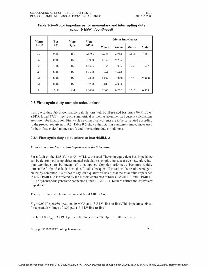
CALCULATING AC SHORT-CIRCUIT CURRENTS IEEEIN ACCORDANCE WITH ANSI-APPROVED STANDARDS Std 551-2006
Copyright © 2006 IEEE. All rights reserved. 219
9.8 First cycle duty sample calculations
First cycle duty ANSI-compatible calculations will be illustrated for buses 04:MILL-2,
8:FDR L and 37:T14 sec. Both symmetrical as well as asymmetrical current calculations
are shown for illustration. First cycle asymmetrical currents are to be calculated according
to the procedures given in 9.5. Table 9-2 shows the rotating equipment impedances used
for both first cycle (“momentary”) and interrupting duty simulations.
9.8.1 First cycle duty calculations at bus 4:MILL-2
Fault current and equivalent impedance at fault location
For a fault on the 13.8 kV bus 04: MILL-2 the total Thevenin equivalent bus impedance
can be determined using either manual calculations employing successive network reduc-
tion techniques or by means of a computer. Complex arithmetic becomes rapidly
intractable for hand-calculations, thus for all subsequent illustrations the results were gen-
erated by computer. It suffices to say, on a qualitative basis, that the total fault impedance
to bus 04:MILL-2 is affected by the motors connected at buses 03:MILL-1 and 04:MILL-
2. The synchronous generator connected at bus 03:MILL-1, reduces further the equivalent
impedance.
The equivalent complex impedance at bus 4:MILL-2 is,
Zeq = 0.0017 +j 0.0301 p.u., on 10 MVA and 13.8 kV (line-to-line).This impedance gives,
for a prefault voltage of 1.00 p.u. (13.8 kV line-to-line)
I3-ph = 1.00/Zeq = 33.1971 p.u. at –86.74 degrees OR I3ph = 13 889 amperes,
37 0.48 IM 0.6788 0.246 2.952 0.615 7.381
37 0.48 IM 0.3000 1.859 9.296
39 4.16 IM 1.6625 0.034 1.005 0.051 1.507
49 0.48 IM 1.2500 0.264 2.640
51 0.48 IM 0.2000 1.432 10.020 3.579 25.050
51 0.48 IM 0.5700 0.408 4.893
8 13.80 SM 9.0000 0.006 0.222 0.010 0.333
Table 9-2—Motor impedances for momentary and interrupting duty
(p.u., 10 MVA) (continued)
Motor bus #
BuskV
Motortype
MotorMVA
Motor impedances
Rmom Xmom Rinter Xinter
Authorized licensed use limited to: UNIVERSIDADE DE SAO PAULO. Downloaded on September 14,2020 at 17:33:56 UTC from IEEE Xplore. Restrictions apply.

IEEEStd 551-2006 CHAPTER 9
220 Copyright © 2006 IEEE. All rights reserved.
while the separate X and R reductions yielded an X/R ratio of 22.363. This ratio is calcu-
lated as the ratio of total equivalent reactance of 0.030 p.u as calculated from the reactance
network and the total equivalent resistance of 0.00134 p.u. as calculated from the resis-
tance network. Note that if the X/R were calculated from the equivalent complex
impedance the result would have been 17.70 (= 0.0301/0.0017).
First-ring fault current contributions for a fault at 4:MILL-2
Table 9-3 illustrates the composition of the total fault current at bus 4:MILL-2 as contribu-
tions from the buses located one-bus away from the fault location.
Asymmetrical first cycle fault currents
For X/R ratios calculated according to ANSI-procedures following separate X and Rreductions, Table 9-4 depicts the first cycle currents at bus 4:MILL-2 that can be quanti-
fied as either total asymmetrical rms or peak currents.
Table 9-3—First ring contributions for a fault at bus 4:MILL-2 (first cycle)
From busCurrent
(p.u.)Current
(A)Angle (deg)
Fault MVA
2:69-2 15.2533 6381 –85.66 153
15:FDR I 1.3157 550 –86.35 13
16:T9 PRI 0.2170 91 –84.12 2
24:FDR M 1.3038 545 –86.05 13
27:T12 PRI 0.8788 367 –82.13 9
8:FDR L 4.4792 1874 –88.15 45
GEN2 9.7618 4084 –88.40 97.6
Table 9-4—First cycle asymmetrical currents at bus 4:MILL-2
Bus 4:MILL-2, first cycle ANSI X/R=22.363 Isym = 13 889 A
Total 1/2 cycle asymmetrical rms, per 1.6 multiplier Iasym = 22 2205 A
Total 1/2 cycle asymmetrical rms, per ANSI equation Iasym = 22 000 A
Peak current based on 2.6 multiplier Ipeak = 36 110 A
Peak current, per “Violet book” equation (2.644 multiplier) Ipeak = 36 730 A
Authorized licensed use limited to: UNIVERSIDADE DE SAO PAULO. Downloaded on September 14,2020 at 17:33:56 UTC from IEEE Xplore. Restrictions apply.

CALCULATING AC SHORT-CIRCUIT CURRENTS IEEEIN ACCORDANCE WITH ANSI-APPROVED STANDARDS Std 551-2006
Copyright © 2006 IEEE. All rights reserved. 221
9.8.2 First cycle duty calculations at bus 8:FDR L
Fault current and equivalent impedance at fault location
For a fault at the 13.8 kV bus 8:FDR L, the equivalent complex impedance reads as
follows:
Zeq = 0.0023 + j 0.0307 p.u., on 10 MVA and 13.8 kV (line-to-line).This impedance gives,
for a prefault voltage of 1.00 p.u. (13.8 kV line-to-line)
I3-ph = 1.00/Zeq = 32.4356 p.u. at –85.80 degrees OR I3ph = 13 570 amperes,
while the separate X and R reductions yielded an X/R ratio of 17.513. This ratio is calcu-
lated as the ratio of total equivalent reactance of 0.031 p.u. (as calculated from the
reactance network) and the total equivalent resistance of 0.00177 p.u. (as calculated from
the resistance network). Note that if the X/R were calculated from the equivalent complex
impedance the result would have been 13.35 (= 0.0307/0.0023).
First-ring fault current contributions for a fault at 8:FDR L
Table 9-5 illustrates the composition of the total fault current at bus 8:FDR L as contribu-
tions from the bus 4:MILL-2 and the 9 MVA synchronous motor M-FDR-L connected
directly at the bus.
Asymmetrical first cycle fault currents
For X/R ratios calculated according to ANSI-procedures following separate X and Rreductions, Table 9-6 depicts the first cycle currents at bus 8:FDR L that can be quantified
as either total asymmetrical rms or peak currents.
Table 9-5—First ring contributions for a fault at bus 8:FDR L
From busCurrent
(p.u.)Current
(A)Angle (deg)
FaultMVA
4:MIIL-2 27.9426 11690 –85.40 279
MOTOR 4.4981 1882 –88.34 45
Table 9-6—Fist-cycle asymmetrical currents at bus 8:FDR L
Bus 8:FDR L, first cycle ANSI X/R=17.513 Isym = 13.57 KA
Total 1/2 cycle asymmetrical rms, per 1.6 multiplier Iasym = 21.71 KA
Total 1/2 cycle asymmetrical rms, per ANSI equation Iasym = 21.01 KA
Authorized licensed use limited to: UNIVERSIDADE DE SAO PAULO. Downloaded on September 14,2020 at 17:33:56 UTC from IEEE Xplore. Restrictions apply.

IEEEStd 551-2006 CHAPTER 9
222 Copyright © 2006 IEEE. All rights reserved.
9.8.3 First cycle duty calculations at bus 37:T14 SEC
Fault current and equivalent impedance at fault location
For a fault at the low-voltage bus 37:T14 SEC, the equivalent complex impedance reads as
follows:
Zeq = 0.0776 + j 0.4726 p.u., on 10 MVA and 13.8 kV (line-to-line)
This impedance gives, for a prefault voltage of 1.00 p.u. (13.8KV line-to-line)
I3-ph = 1.00/Zeq = 2.088 p.u. at –80.68 degrees OR I3ph = 25 115 amperes,
while the separate X and R reductions yielded an X/R ratio of 6.607. This ratio is, again,
calculated as the ratio of total equivalent reactance of 0.472 p.u. (as calculated from the
reactance network) and the total equivalent resistance of 0.0714 p.u. (as calculated from
the resistance network). Note that if the X/R were calculated from the equivalent complex
impedance the result would have been 6.09 (= 0.4726/0.0776).
First-ring fault current contributions for a fault at 37:T14 SEC
Table 9-7 illustrates the composition of the total fault current at bus 37:T14 SEC as contri-
butions from the bus 32:FDR Q and the induction motors directly connected at this bus.
Asymmetrical first cycle fault currents at 37:T14 SEC
For X/R ratios calculated according to ANSI-procedures following separate X and Rreductions, Table 9-8 depicts the first cycle currents at bus 37:T14 SEC that can be quanti-
fied as either total asymmetrical rms or peak currents.
Peak current based on 2.7 multiplier Ipeak = 35.28 KA
Peak current, per “Violet book” equation (2.598 multiplier) Ipeak = 35.26 KA
Table 9-7—First ring contributions for a fault at bus 37:T14 SEC
From busCurrent
(p.u.)Current
(A)Angle (deg)
Fault MVA
37:T14 SEC 1.6462 19801 –79.87 16
M-T14-2 0.1055 1269 –78.69 1
M-T14-1 0.3376 4060 –85.24 3
Table 9-6—Fist-cycle asymmetrical currents at bus 8:FDR L
Authorized licensed use limited to: UNIVERSIDADE DE SAO PAULO. Downloaded on September 14,2020 at 17:33:56 UTC from IEEE Xplore. Restrictions apply.

CALCULATING AC SHORT-CIRCUIT CURRENTS IEEEIN ACCORDANCE WITH ANSI-APPROVED STANDARDS Std 551-2006
Copyright © 2006 IEEE. All rights reserved. 223
From the above-illustrated results, it is seen that the separate X/R reduction yields a larger
fault-point X/R ratio, something that is to be expected in most practical applications. It is
also seen that the complex network reduction, for the same buses, results in a slightly
higher resistance as compared to the resistance calculated from the separate R reduction,
while the reactance values remain comparable. These patterns are consistent with regu-
larly observed practice, and found to be typical with ANSI-calculated X/R ratios.
It is also seen that both total half-cycle asymmetrical rms and peak currents are quite sen-
sitive to the X/R ratio. In fact, lower asymmetrical current estimates would have been
obtained if lower X/R ratios had been used. Furthermore, using the 1.6 and 2.6 multipliers
for a quick estimation of total 1/2 asymmetrical rms and peak currents respectively can be
non-conservative for some cases.
9.9 Interrupting duty sample calculations
In this subclause, interrupting duty ANSI-compatible calculations will supplement the
first cycle simulations performed for buses 04:MILL-2 and 8:FDR L. Symmetrical and
asymmetrical short-circuit currents calculations are shown for illustration.
First cycle calculations suffice for bus 37:T14 SEC, since low-voltage interrupting equip-
ment rating structures for instantaneously-acting devices like fuses and LVCBs equipped
with instantaneous elements do not necessitate dedicated interrupting duty calculations. If
the low-voltage breakers, however, had short time trips without an instantaneous trip ele-
ment, then an extended time or '30 cycle' fault calculation should be made if the first cycle
fault current is over the breaker short time rating.
9.9.1 Interrupting duty calculations for bus 4:MILL-2
Equivalent impedance, fault current and fault MVA at fault location
Zeq = 0.0019 +j 0.0337 p.u., resulting in a symmetrical rms three-phase fault current of
12 407 amperes with an angle of –86.85 degrees for a prefault voltage of 1.00
p.u.(13.8 kV line-to-line). For this current, the three-phase fault MVA level is found to be
297 MVA.
X/R ratio and impedances
The separate X and R reduction resulted in an equivalent reactance Xeq = 0.034 p.u. and an
equivalent resistance of 0.00149 p.u., thus yielding an X/R ratio of 22.8 (= 0.034/0.00149)
Table 9-8—First cycle asymmetrical currents at bus 37:T14 SEC
Bus 37:T14 SEC, first cycle ANSI X/R = 6.607 Isym = 25,115 A
Total 1/2 cycle asymmetrical rms, per ANSI equation Iasym = 33,439 A
Peak current per “Violet book” equation Ipeak = 58,042 A
Authorized licensed use limited to: UNIVERSIDADE DE SAO PAULO. Downloaded on September 14,2020 at 17:33:56 UTC from IEEE Xplore. Restrictions apply.

IEEEStd 551-2006 CHAPTER 9
224 Copyright © 2006 IEEE. All rights reserved.
First-ring contributions
From bus 2: 69-2 6376 amperes at an angle of –85.67 degrees
From bus 15:FDRI 393 amperes at an angle of –86.49 degrees
From bus 16:T9 PRI 0.0 amperes at an angle of 0.00 degrees
From bus 24: FDR M 236 amperes at an angle of –87.13 degrees
From bus 27:T12 PRI 71 amperes at an angle of –81.55 degrees
From bus 8:FDR L 1251 amperes an angle of –88.21 degrees
From generator GEN2 4084 amperes at an angle of –88.40 degrees
Generator contribution classification
Once the contributions have been calculated, the synchronous generator contributions
need to be classified as either “local” or “remote”. The following table illustrates the clas-
sification process according to the 40% criterion, as outlined in 9.4. Next to the p.u.
contribution of every generator is also shown in parenthesis the comparison threshold
according to which the classification is made. The threshold, for every generator, is 40%
of the fault current one would obtain if the generator terminals were boldly faulted.
According to Table 9-9, the fault current featuring no ac decrement is approximately
15.082 p.u (14.073 + 1.009 p.u), amounting to 50.855% of the total fault current. Com-
puter calculations taking into account vectorial arithmetic yielded a total of 50.90%,
amounting to a NACD content of 0.509. All motor contributions were considered “local”
for this calculation.
Calculation of asymmetrical currents for totally rated breakers
Let us assume for illustration that a 5-cycle totally rated breaker is to be applied. Assum-
ing a breaker contact parting time of 3 cycles, for a fault point X/R ratio of 22.797, one
obtains for a three-phase fault a “remote” multiplier of 1.175 and a “local” multiplier of
1.07 from Figure 9-1a and Figure 9-1b respectively. We therefore, obtain the following:
Table 9-9—Generator contribution classification for fault at 4:MILL-2
Fault at bus 4:MILL-2 Fault current (p.u.) 29.6564
Current from Utility (Remote) 14.073 p.u. (by definition)
Current from GEN1 (Remote) 1.009 p.u. (< 5.5784 p.u)
Current form GEN2 (Local) 9.762 p.u (> 3.9048 p.u)
Authorized licensed use limited to: UNIVERSIDADE DE SAO PAULO. Downloaded on September 14,2020 at 17:33:56 UTC from IEEE Xplore. Restrictions apply.

CALCULATING AC SHORT-CIRCUIT CURRENTS IEEEIN ACCORDANCE WITH ANSI-APPROVED STANDARDS Std 551-2006
Copyright © 2006 IEEE. All rights reserved. 225
Iasym = 12 407 (1.175) = 14 578 A (remote multiplier only)
Iasym = 12.407 (0.491)(1.07) + 12 407(1.175)(0.509) = 13 939 A (weighted)
And following the equivalent NACD ratio approach:
12 407 [(1.175 – 1.07)(0.509) + 1.07] = 13 939 amperes
Calculation of asymmetrical currents for symmetrically rated breakers
Let us assume for illustration that a 5-cycle symmetrically rated breaker is to be applied.
Assuming, again, a breaker contact parting time of 3 cycles, for a fault point X/R ratio of
22.797, one obtains for a three-phase fault a “remote” multiplier of 1.068 and a “local”
multiplier of 1.00, see Figure 9-2a and Figure 9-2b respectively. We therefore, obtain the
following:
Iasym = 12 407 (1.068) = 13 251 A (remote multiplier only)
Iasym = 12.407 (0.491)(1.00) + 12 407(1.068)(0.509) = 12 836 A (weighted)
And following the equivalent NACD ratio approach:
12 407 [(1.068-1.00)(0.509) + 1.00] = 12 836 amperes
9.9.2 Interrupting duty calculations for bus 8:FDR L
Equivalent impedance, fault current, and fault MVA at fault location
Complex network reduction for bus 8:FDR E yielded an equivalent complex impedance of
Zeq = 0.0024 +j 0.0344 p.u., resulting in a symmetrical rms three-phase fault current of
12 130 amperes with an angle of –85.93 degrees for a prefault voltage of 1.00 p.u.
(13.8 kV line-to-line). For this current, the three-phase fault MVA level is found to be 290
MVA.
ANSI X/R ratio and impedances
The separate X and R reduction resulted in an equivalent reactance Xeq=0.034 p.u. and an
equivalent resistance of 0.00195 p.u., thus yielding an ANSI X/R ratio of 17.434 (= 0.034/
0.00195)
First-ring contributions
From bus 4: MILL-2 10 877 amperes at an angle of –85.65 degrees
From MOTOR M-FDR-L 1255 amperes at an angle of –88.34 degrees
Authorized licensed use limited to: UNIVERSIDADE DE SAO PAULO. Downloaded on September 14,2020 at 17:33:56 UTC from IEEE Xplore. Restrictions apply.

IEEEStd 551-2006 CHAPTER 9
226 Copyright © 2006 IEEE. All rights reserved.
Generator contribution classification
Once the contributions have been calculated, the synchronous generator contributions
need to be classified as either “local” or “remote.” The following table illustrates the clas-
sification process according to the 40% criterion, as outlined in 9.4. Next to the p.u.
contribution of every generator is also shown in parentheses the comparison threshold
according to which the classification is made. The threshold, for every generator, is 40%
of the fault current one would obtain if the generator terminals were boldly faulted.
According to Table 9-10, the fault current featuring no ac decrement is approximately
14.704 p.u (13.720 p.u. + 0.984 p.u), amounting to approximately 50.7% of the total fault
current. Computer calculations taking into account vectorial arithmetic yielded a total of
50.70%, amounting to a NACD content of 0.507. All motor contributions were, again,
considered “local” for this calculation.
Calculation of asymmetrical currents for totally rated breakers
Let us assume for illustration that a three-cycle totally rated breaker is to be applied.
Assuming a breaker contact parting time of two cycles, for a fault point X/R ratio of
17.434, one obtains for a three-phase fault a “remote” multiplier of 1.214 and a “local”
multiplier of 1.149 from Figure 9-1a and Figure 9-1b respectively. We therefore, obtain
the following:
Iasym = 12 130 (1.214) = 14 726 A (remote multiplier only)
Iasym = 12 130(0.493)(1.149) + 12 130(1.214)(0.507) = 14 337 A (weighted)
And following the equivalent NACD ratio approach:
12 130 [(1.214–1.149)(0.507)+1.149] = 14 337 amperes
Calculation of asymmetrical currents for symmetrically rated breakers
Let us assume for illustration that a three-cycle symmetrically rated breaker is to be
applied. Assuming, again, a breaker contact parting time of 2 cycles, for a fault point X/Rratio of 17.434, one obtains for a three-phase fault a “remote” multiplier of 1.012 and a
Table 9-10— Generator contribution classification for a fault at 8:FDR L
Fault at bus 8:FDR L Fault current (p.u.) 28.9935
Current from Utility (Remote) 13.720 p.u. (By definition)
Current from GEN1 (Remote) 0.984 p.u. (< 5.5784 p.u)
Current form GEN2 (Local) 9.517 p.u (> 3.9048 p.u)
Authorized licensed use limited to: UNIVERSIDADE DE SAO PAULO. Downloaded on September 14,2020 at 17:33:56 UTC from IEEE Xplore. Restrictions apply.

CALCULATING AC SHORT-CIRCUIT CURRENTS IEEEIN ACCORDANCE WITH ANSI-APPROVED STANDARDS Std 551-2006
Copyright © 2006 IEEE. All rights reserved. 227
“local” multiplier of 1.00 from Figure 9-2a and Figure 9-2b respectively. We therefore,
obtain:
Iasym = 12 130 (1.012) = 12 276 A (remote multiplier only)
Iasym = 12.130 (0.493)(1.00) + 12 130(1.012)(0.507) = 12 204 A (weighted)
And following the equivalent NACD ratio approach:
12 130 [(1.012 – 1.00)(0.507) + 1.00] = 12 204 amperes
It is seen that using a “remote” multiplier only, the asymmetrical current estimate is higher
(more conservative) as compared to the value obtained using a “weighted” approach. This
is true for either breaker rating structure. If there is no in-plant generation at all in the
industrial system, it is common practice to use the “remote” multiplying factors only.
Considering the motor contribution as “remote” would also yield more conservative
(higher) asymmetrical fault current estimates.
The classification of the generating station contributions as either “local” or “remote” is a
non-trivial calculation, particularly for systems featuring many generators and non-radial
topology. These calculations are greatly facilitated by today’s computer programs, which
automate these procedures and criteria for any faulted bus, by virtue of well-established
analytical techniques (Anderson [B1]). Another advantage of modern-vintage commer-
cial-grade computer software, designed to support ANSI-conformable calculations, is the
ability to view the system-wide effects, both voltage-wise on the system buses and cur-
rent-wise on any branch or source, for any phase or sequence, when simulating a fault at
any location. Figure 9-5 illustrates such a typical graphical report, portraying the system
state in p.u. something that permits immediate qualitative assessment of the effects of the
fault and inspection of the synchronous generator contribution levels. A rather local view
is illustrated here, but “zoom” and “pan” facilities should render any part of the single line
diagram available for closer inspection. An equally important and “sought-after” attribute
of any computer-generated result, besides flexibility and convenience, should be to pro-
Authorized licensed use limited to: UNIVERSIDADE DE SAO PAULO. Downloaded on September 14,2020 at 17:33:56 UTC from IEEE Xplore. Restrictions apply.

IEEEStd 551-2006 CHAPTER 9
228 Copyright © 2006 IEEE. All rights reserved.
vide enough information so that all valid interpretations of the ANSI-related calculations
can be applied with ease.
9.10 Applying ANSI calculations to non-60 Hz systems
ANSI calculating procedures for interrupting requirements purposes can be applied to sys-
tem other than 60 Hz. The interrupting equipment manufacturer should, in principle,
determine if the equipment can be applied to system frequencies for which it was not
originally designed for. For example, most of the breaker and fuse equipment manufac-
tured in the U.S. have a nominal design frequency of 60 Hz, but they are sometimes
applied on 50-Hz systems. The three critical factors to keep in mind for equipment ratings
and calculating procedures in non-60 Hz systems are asymmetry factor for the first half
cycle, contact parting time of high-voltage breakers and the system X/R ratio.
9.10.1 Asymmetry factor equations
The previously defined equations for calculating first cycle peak and 1/2 cycle asymmetri-
cal rms fault remain, in principle, valid for non-60 Hz systems. They both involve either
breaker parting time OR system X/R ratio for 60 Hz. The fact remains, however, that both
time in cycles of the new frequency as well as the reactance for the new frequency must be
consistent.
Figure 9-5—Typical computer-generated, system-wide graphical report for
Interrupting duty calculations (three-phase fault at bus 4: MILL-2)
Authorized licensed use limited to: UNIVERSIDADE DE SAO PAULO. Downloaded on September 14,2020 at 17:33:56 UTC from IEEE Xplore. Restrictions apply.

CALCULATING AC SHORT-CIRCUIT CURRENTS IEEEIN ACCORDANCE WITH ANSI-APPROVED STANDARDS Std 551-2006
Copyright © 2006 IEEE. All rights reserved. 229
9.10.2 Breaker contact-parting times and X/R ratio
The contact parting time of a breaker, in seconds, is a function of breaker mechanics and
does not change when the breaker is applied on a frequency other than 60 Hz, but the
breaker contact-parting time in cycles does change. The techniques for obtaining the
“remote” multiplying factors, tabular and analytical, remain valid for other than 60 Hz fre-
quencies provided, again, that the contact-parting time and the X/R ratio are correct and
consistent for the new frequency.
The previously defined “local” multiplying factors may still apply provided that the con-
tact parting time in cycles and the X/R ratio remain consistent for the new frequency.
Whenever applying dc decrement characteristics from IEEE Std C37.010 it should be
remembered that they are still valid but for an X/R ratio of 14 when the system frequency
is 50 Hz.
9.11 Normative references
The following referenced documents are indispensable for the application of this docu-
ment. For dated references, only the edition cited applies. For undated references, the
latest edition of the referenced document (including any amendments or corrigenda)
applies.
ANSI C37.5, Guide for Calculation of Fault Currents for Application of AC High-Voltage
Circuit Breakers Rated on a Total Current Basis.3
IEEE Std C37.010™, IEEE Application Guide for AC High-Voltage Circuit Breakers
Rated on a Symmetrical Current Basis.4, 5
IEEE Std C37.13™, IEEE Standard for Low-voltage AC Power Circuit Breakers Used in
Enclosures.
IEEE Std 141™, IEEE Recommended Practice for Electric Power Distribution for Indus-
trial Plants. (IEEE Red Book)
IEEE Std 241™, IEEE Recommended Practice for Electric Power Systems for Commer-
cial Buildings. (IEEE Gray Book)
IEEE Std 242™, IEEE Recommended Practice for Protection and Coordination of Indus-
trial and Commercial Power systems. (IEEE Buff Book)
3ANSI C37.5 has been withdrawn; however, copies can be obtained from the Sales Department, American National Standards Institute, 25 West 43rd Street, 4th Floor, New York, NY 10036, USA (http://www.ansi.org/).4IEEE publications are available from the Institute of Electrical and Electronics Engineers, 445 Hoes Lane, P.O.Box 1331, Piscataway, NJ 08855-1331, USA (http://standards.ieee.org/).5The IEEE standards or products referred to in this subclause are trademarks of the Institute of Electrical andElectronics Engineers, Inc.
Authorized licensed use limited to: UNIVERSIDADE DE SAO PAULO. Downloaded on September 14,2020 at 17:33:56 UTC from IEEE Xplore. Restrictions apply.

IEEEStd 551-2006 CHAPTER 9
230 Copyright © 2006 IEEE. All rights reserved.
9.12 Bibliography
[B1] Anderson, Paul, Analysis of Faulted Power Systems, IEEE Power System Engineer-
ing Series, IEEE Press 1995.
[B2] Blackburn, L .J. Symmetrical Components for Power Systems Engineering, New
York, Marcel Dekker, Inc., 1993.
[B3] Huening, W. C., “Calculating Short-Circuit Currents with contributions from induc-
tion motors,” IEEE Transactions on Industry and General Applications, Vol. IA-18, pp.
85-92, Mar/Apr 1982.
[B4] Huening, W .C. “Interpretation of New American National Standards for Power Cir-
cuit Breaker Applications.” IEEE Transactions on Industry and General Applications,Vol IGA-5, Sept/Oct,1969.
[B5] Stevenson, W. D. Elements of Power System Analysis, New York, McGraw-Hill,
1982.
[B6] Wagner, C. F., Evans, R.D. Symmetrical Components, New York, McGraw-Hill,
1933.
Authorized licensed use limited to: UNIVERSIDADE DE SAO PAULO. Downloaded on September 14,2020 at 17:33:56 UTC from IEEE Xplore. Restrictions apply.

Copyright © 2006 IEEE. All rights reserved. 231
Chapter 10Application of short-circuit interrupting equipment
10.1 Introduction
This chapter describes the application of electrical power system interrupting equipment
for three-phase and line-to-ground short-circuit currents. The fault currents used are from
the one-line diagram used throughout this book and includes generator, induction and
synchronous motors contributions. The application of interrupting equipment, in some
cases, requires more than comparing an interrupting current given on the nameplate to the
calculated duty. The calculation of fault currents in accordance to ANSI-approved
standards are covered in Chapter 9. The term duty as used in this text is the maximum
symmetrical fault current times any multipliers, which makes the resulting current directly
comparable with the equipment rating.
10.2 Purpose
The objective of this chapter is to give examples of taking available interrupting
equipment data and making comparisons to the calculated short-circuit duty. The
capability of the interrupting equipment to adequately interrupt short-circuit currents is a
safety as well as a system and equipment protection consideration. The National Electrical
Code® (NEC®) (NFPA 70, 2005 Edition)1 states that “Equipment intended to break
current at fault levels shall have an interrupting rating sufficient for the nominal circuit
voltage and the current that is available at the line terminals of the equipment.” (See NEC,
Section 110-9.) “The overcurrent protective devices, the total impedance, the component
short-circuit withstand ratings, and other characteristics of the circuit to be protected shall
be so selected and coordinated as to permit the circuit protective devices that are used to
clear a fault without the occurrence of extensive damage to the electrical components of
the circuit.” (See NEC, Section 110-10.)
10.3 Application considerations
Once a short-circuit calculation has been made using the best data available, the
application or verification of breaker, fuse, switches, and other equipment ratings needs to
be made. Subclause 10.7 provides a list on equipment that may have to be checked against
the short-circuit fault currents. Depending on the purpose of the fault calculations not all
equipment given in 10.7 list will need to be checked. A number of items from the short-
circuit calculations have to be considered when comparing the fault currents against the
equipment. These are as follows:
1) Circuit voltage
2) Circuit fault current
3) Fault current X/R ratio
1Information on normative references can be found in 10.12.
Authorized licensed use limited to: UNIVERSIDADE DE SAO PAULO. Downloaded on September 14,2020 at 17:33:56 UTC from IEEE Xplore. Restrictions apply.

IEEEStd 551-2006 CHAPTER 10
232 Copyright © 2006 IEEE. All rights reserved.
4) Equipment first cycle withstand capabilities
5) Equipment first cycle interrupting current capabilities
6) Equipment interrupting time and current capabilities
7) Equipment maximum application voltage and maximum interrupting current
8) Equipment minimum application voltage and minimum interrupting current
9) Equipment interrupting test X/R ratio
10) Non-interrupting equipment fault current withstand and thermal capabilities
Several methods are used to modify the fault current or breaker rating when a multiplier is
required because of system conditions. A derating factor can be applied to the interrupting
device rating or a multiplier can be applied to the current. In this book the latter will be
used. In general the multiplier on the current is preferred because the interrupting
equipment ratings will remain the same for all buses at the same voltage. Otherwise, the
adjusted interrupting equipment current ratings may differ depending on the fault current
X/R ratio.
Given in Table 10-1 are the general test X/R ratios of interrupting equipment.
Table 10-1—Minimum test X/R ratios
Type of equipmentFirst cycle
currentFirst cycle X/R
Interrupting time or short
time X/R
Low-voltage power circuit breaker(iron frame breaker)
Peak 6.59 6.59
Low-voltage molded and insulated casebreakers with interrupting ratings > 20 kA
Peak 4.9 4.9
Low-voltage molded and insulated casebreakers with interrupting ratings 10-20 kA
Peak 3.18 3.18
Low-voltage molded and insulated casebreakers with interrupting ratings < 10 kA
Peak 1.73 1.73
Fused low-voltage power circuit breakers Peak 4.9 4.9
Low-voltage busway Peak 4.9 4.9
High-voltage power circuit breaker rms 25 15
Power fuse rms 15 —
Distribution fuse rms 10 —
Distribution air cutout fuse rms 5–15 depends on kV rating
—
Distribution oil cutout fuse rms 9–12 depends on kV rating
—
Authorized licensed use limited to: UNIVERSIDADE DE SAO PAULO. Downloaded on September 14,2020 at 17:33:56 UTC from IEEE Xplore. Restrictions apply.

IEEEAPPLICATION OF SHORT-CIRCUIT INTERRUPTING EQUIPMENT Std 551-2006
Copyright © 2006 IEEE. All rights reserved. 233
10.4 Equipment data
Equipment rating data for a particular type of equipment can vary over several years of
manufacture depending upon improvements in the equipment, special limitation of the
equipment, or changes in the rating structure. The recommended ratings and required data
to be placed on equipment nameplates is given in the appropriate ANSI, IEEE, and
NEMA standards for the equipment. Short-circuit test requirements given by NEMA,
Underwriters Laboratories, ANSI, or IEEE are generally the same for the type of
equipment involved. Not all manufacturers follow the standards’ recommended rating
structure. Some interrupting equipment may be sized to fit an area not covered by the
standards or the equipment may have a higher or lower interrupting capability than
suggested by the standard recommended ratings system.
Several examples of equipment rating changes are given below. The broad range of GE
type AM-13.8-500 medium-voltage class of breakers used in metal-clad switchgear covers
many years. During the years of manufacture, the ANSI rating structure was revised and
the breaker design was changed to accommodate the change. In the mid-60s the breaker
design and nameplate reflected the ANSI change of total current method of testing to the
symmetrical current method of testing. Unless additional data is furnished, (Series No.,
year of manufacture, complete nameplate data) there is no way to determine the actual
rating of the breaker. A second example is the BBC type xx-HK-xxx medium-voltage
class of breakers rated on a symmetrical current basis have a 5 cycle interrupting time.
However, the breaker nameplate and literature gives a 1.2 asymmetry factor. This
information indicates that the breaker has a 2-cycle contact parting time rather than the
three cycles contact parting normally associated with 5-cycle interrupting time breakers. A
third case is that S&C power fuses literature provides varying symmetrical interrupting
ratings depending upon the system fault X/R ratio. Normally most manufacturers of power
fuses provide only one interrupting rating at an X/R ratio of 15.
Based on the previous discussion, rating variations from different vendors are possible and
care should be exercised in using general equipment data. The preference order of
obtaining equipment data is as follows as follows:
1) Equipment nameplate
2) Manufacturer’s literature
3) ANSI, IEEE, or NEMA standards
Switches (withstand rating) rms 25 —
High-voltage bus duct 25 —
Table 10-1—Minimum test X/R ratios (continued)
Type of equipmentFirst cycle
currentFirst cycle X/R
Interrupting time or short
time X/R
Authorized licensed use limited to: UNIVERSIDADE DE SAO PAULO. Downloaded on September 14,2020 at 17:33:56 UTC from IEEE Xplore. Restrictions apply.

IEEEAPPLICATION OF SHORT-CIRCUIT INTERRUPTING EQUIPMENT Std 551-2006
Copyright © 2006 IEEE. All rights reserved. 234
10.5 Fully-rated systems
In a fully-rated system, all interrupting equipment is applied to interrupt the total fault
current at the point of the fault. All high-voltage breakers require a fully-rated system. All
low-voltage power circuit breakers (iron frame) require a fully-rated system. All low-
voltage systems greater than 480 volts require a fully-rated system.
The use of first half cycle current-limiting interrupting devices on a high-voltage system
to reduce the amount of fault current the breakers have to interrupt is not covered by the
standards. The manufacturer of a breaker used in such a manner should be consulted to
determine its acceptability and change in warranty, if any.
Section 110-9 of the NEC requires that fault interrupting devices have an interrupting
rating sufficient to withstand the current to be interrupted. This is commonly known as a
fully-rated system. However, low-voltage series rated equipment is allowed.
10.6 Low-voltage series rated equipment
Series rating on equipment allows the application of two series interrupting devices for a
condition where the available fault current is greater than the interrupting rating of the
downstream equipment. Both devices share in the interruption of the fault and selectivity
is sacrificed at high fault levels. Selectivity should be maintained for tripping currents
caused by overloads.
The NEC states “If a circuit breaker is used on a circuit having an available fault current
higher than its marked interrupting rating by being connected on the load side of an
acceptable overcurrent protective device having the higher rating..., this series
combination rating shall be marked on the end use equipment.” (See NEC,Section 249-6.)
In this case, the short-circuit rating assigned to the combination of the series devices can
be higher than the lowest downstream rated device of the combination.
In a series combination of fuses or breakers, series rated equipment must meet some strict
rules in order to be applied.
1) Series rated combinations should be selected by a registered professional engineer
whose primary occupation is the design and maintenance of electrical installa-
tions. The design documents should be stamped with the seal of the professional
engineer.
2) A series combination is recognized for series application by a third-party
organization such as UL. UL 489-2002 outlines the test connections and
procedures for proof of series combination ratings. Analytical methods such as the
“up-over-and-down” method for applying fuses may not be used for circuit
breakers that exhibit contact parting in the first half-cycle.
3) The tested combination does not allow for faults closer than four feet from the
load side breaker.
Authorized licensed use limited to: UNIVERSIDADE DE SAO PAULO. Downloaded on September 14,2020 at 17:33:56 UTC from IEEE Xplore. Restrictions apply.

IEEEAPPLICATION OF SHORT-CIRCUIT INTERRUPTING EQUIPMENT Std 551-2006
Copyright © 2006 IEEE. All rights reserved. 235
4) The current in the two interrupting devices must be the same current. Motor fault
current contribution that would allow the downstream breaker to have a higher
current as compared to the upstream breaker/fuse is not allowed.
5) Series ratings apply to systems at 600 V and below.
6) The series rating test has been made at only one power factor, whereas the actual
fault power factor could vary widely.
7) Since the load breaker is subject to higher than rated fault currents, it should be
thoroughly checked and tested after each fault operation.
8) Series ratings apply for selected low-voltage equipment (Molded-case circuit
breakers and current limiting fuses).
9) Upstream devices must have instantaneous trips or clearing times.
10) There is no limitation on physical distance between interrupting devices.
A listing of the tested combinations can be obtained from the UL Recognized Component
Directory (UL-RCD). Usage of series rated protective devices does not lead to a
coordinated selective system but to a protective system, wherein the system reliability is
sacrificed because of the loss of selectivity of protective equipment.
10.7 Low-voltage circuit breaker short-circuit capabilities less than
rating
The ANSI test standard for low-voltage power breakers describes a short-circuit test for
breakers where full line-to-line voltage is applied across an interrupting pole of a breaker.
For this condition, the breaker must be capable of interrupting at least 87% of its three-
phase interrupting rating. For a single phase system where two poles of a three-phase
breaker are used to interrupt the short circuit, the one pole, full voltage, 87% capability
does not apply because each pole “sees” 50% of the line-to-line voltage, which is less than
the normal line-to-neutral voltage of a three-phase system. Using a single pole of a three-
phase breaker to interrupt a single phase line-to-line short circuit requires that the breaker
single pole voltage capability be greater than the normal line-to-neutral voltage of the
system or a reduced interrupting rating will apply.
The most likely cause of an interruption of a line-to-line short circuit by one pole of a
circuit breaker is a double line-to-ground short circuit in a three-phase system that is not
solidly wye grounded, such as an ungrounded system, high resistance grounded system, or
corner of the delta grounded system. Full line-to-line recovery voltage can occur across a
single interrupting pole when one phase is grounded on the source side of a circuit breaker
and another phase is grounded simultaneously on the load side. For a corner of the delta
grounded system, this might be a common occurrence. The situation is less likely to occur
in high resistance grounded or ungrounded systems where operating procedures require
the first ground to be removed as soon as practical.
The single-pole interruption problem should not be a concern with low-voltage power
breaker because they are tested to meet the criteria in IEEE Std C37.010™-1999. The
maximum line-to-line first cycle short-circuit duty is 87% of the three-phase duty in a
three-phase system. If the power circuit breaker is correctly applied for a three-phase
Authorized licensed use limited to: UNIVERSIDADE DE SAO PAULO. Downloaded on September 14,2020 at 17:33:56 UTC from IEEE Xplore. Restrictions apply.

IEEEStd 551-2006 CHAPTER 10
236 Copyright © 2006 IEEE. All rights reserved.
short-circuit duty, then it is correctly applied for the line-to-line duty independent of the
system grounding. The limiting application may be for a line-to-ground fault on a solidly
grounded system where the line-to-ground fault current may be greater than the three-
phase current, e.g., on the secondary of a transformer.
However, the single-pole interrupting ratings assigned to low-voltage molded case or
insulated case circuit breakers may be based on UL or NEMA standard values, which may
be lower than ANSI requirements. If this restricts an application, the manufacturer should
be consulted because single pole tests using voltages and currents higher than literature
values may have been performed, relieving the restriction.
10.8 Equipment checklist for short-circuit currents evaluation
The following is a listing of items that may need to be compared against the calculated
fault levels. Depending on the purpose of the short-circuit study not all items will need to
be checked. The list does show that there are more devices affected by short-circuit than
just interrupting devices such as fuses and breakers.
1) Fuses—Fuse voltage rating and first cycle interrupting current.
2) High-voltage breakers—Voltage rating, first cycle current, interrupting current. A
system rated 4.8 kV often requires equipment rated at 7.2 kV because the upper
limit of some 4.16 kV class of equipment is 4.76 kV.
3) Low-voltage breakers—Voltage rating, first cycle current (Interrupting), short
time current rating if no instantaneous is supplied, and single pole interrupting
rating.
4) Switches—First cycle current for withstand capabilities.
5) Switchgear, motor control centers—First cycle current for bus bracing and molded
case interrupters.
6) Reclosers—Voltage rating, first cycle current, interrupting current.
7) Cable heating limits—First cycle, interrupting, and time delay relay currents. This
check is more important on systems with time delay tripping and where selective
relay operating times are required. The heat generated in the cable during the fault
could over heat the insulation and deteriorate or melt it. Extremely small cable
while within its load rating could act as a fuse under high fault currents.
8) Line heating limits—First cycle, interrupting, and time delay relay currents. This
check is more important on systems with time delay tripping. The heat generated
in the line during the fault could over heat the line causing more sag and possibly
a second fault, injury, or line melt down.
9) Current limiting reactors—First cycle to check the through current. Per
ANSI 57.16, the rms short-circuit should be less than 33.33 times the rated rms
current.
10) Busways and bus ducts—First cycle current to check the bus bracing.
11) Transformers—First cycle and time-delay currents for mechanical and thermal
withstand limits. The transformer overcurrent relays should be set to protect these
limits per ANSI C57.109.
Authorized licensed use limited to: UNIVERSIDADE DE SAO PAULO. Downloaded on September 14,2020 at 17:33:56 UTC from IEEE Xplore. Restrictions apply.

IEEEAPPLICATION OF SHORT-CIRCUIT INTERRUPTING EQUIPMENT Std 551-2006
Copyright © 2006 IEEE. All rights reserved. 237
12) Line carrier frequency wire traps—First cycle and time delay currents for
mechanical and thermal withstand limits. Wire traps can be the limiting item on a
transmission line.
13) Current transformers—First cycle and time delay currents for the mechanical and
thermal withstand limits. High primary currents can cause current transformer
saturation that may affect relay operation.
14) Generators—First cycle line-to-ground fault currents on non-impedance
grounded generators can have line-to-ground fault currents that are greater than
the three-phase fault current. The winding bracing of the generator is based on
three-phase fault currents.
15) Grounding resistors and reactors—Time delay line-to-ground fault currents if not
properly relayed can exceed the short time ratings of generator and transformer
grounding devices.
16) Series capacitors—First cycle fault currents will result in high voltages across the
capacitors that may exceed both the transient current and voltage capability of the
capacitors and its protective surge equipment.
10.9 Equipment phase duty calculations
The following subclause calculates the first cycle and interrupting time fault current duties
on the above listed equipment. The symmetrical fault currents used to calculate the duties
was taken from the computer printout in Chapter 9. Chapter 3 through Chapter 9 provide
the details of the network reduction needed to determine the symmetrical fault currents.
10.9.1 13.8 kV Breakers
The high-voltage breakers on buses 03:MILL-1 and 04:MILL-2 must be evaluated on both
a first cycle and interrupting time bases. The first cycle duty is compared against the
“close and latch” rating of the symmetrical rated breakers and the “momentary” rating of
the total current rated breakers. The total symmetrical 03:MILL-1 bus fault current is
13.952 kA and the maximum current that a breaker on that bus can see is that for
breaker G, the smallest bus current contribution. The breaker current is 13.837 – 0.179 =
13.658 kA symmetrical. Since the breaker duty is 98.7% of the bus duty, the more
conservative bus fault currents will be used as breaker duties.
Some of the more recent breakers also have a peak current given on the nameplate for the
close and latch rating. This peak rating is 2.7 times the breaker maximum interrupting
current.
The first cycle test X/R for these breakers is 25 and Table 10-2 provides the comparisons
of duty to ratings. The equation for the first cycle rms asymmetrical current is shown in
Equation (10-1):
(10.1)τ 0.49 0.1e
X3R-------–
–=
Authorized licensed use limited to: UNIVERSIDADE DE SAO PAULO. Downloaded on September 14,2020 at 17:33:56 UTC from IEEE Xplore. Restrictions apply.

IEEEAPPLICATION OF SHORT-CIRCUIT INTERRUPTING EQUIPMENT Std 551-2006
Copyright © 2006 IEEE. All rights reserved. 238
(10.2)
The interrupting breaker duty requires additional information concerning the speed of the
breaker, the test procedure used for the breaker at the time of manufacture, total
symmetrical fault current, fault current X/R ratio, and the amount of current from nearby
generators. Chapter 9 went into detail on calculating the amount of current from each
generator, therefore to avoid repeating this detail, the currents will be taken directly from
the computer printout. For each fault, the amount of the generator current considered
“local” from each will have to be determined. When the generator fault current is greater
than 40% of a generator terminal fault current, then the current is considered “local.” The
listing below summaries these findings at the bus fault voltage.
Table 10-2—First cycle evaluation
Bus BreakerFault X/R
Sym. kA
Multi-plier
Duty asym.
kA
Breaker rating
kA
Bus kA bracing
03:MILL-1 AM-13.8-500-3
17.32 13.837 1.550 21.45 40 40
03:MILL-1 VB-13.8-500-1
17.32 13.837 1.550 21.45 38 40
04:MILL-2 15-HK-500 22.29 13.888 1.587 22.04 40 40
Irms Isym 1 2e
2πτRX
-------------–
+=
Authorized licensed use limited to: UNIVERSIDADE DE SAO PAULO. Downloaded on September 14,2020 at 17:33:56 UTC from IEEE Xplore. Restrictions apply.
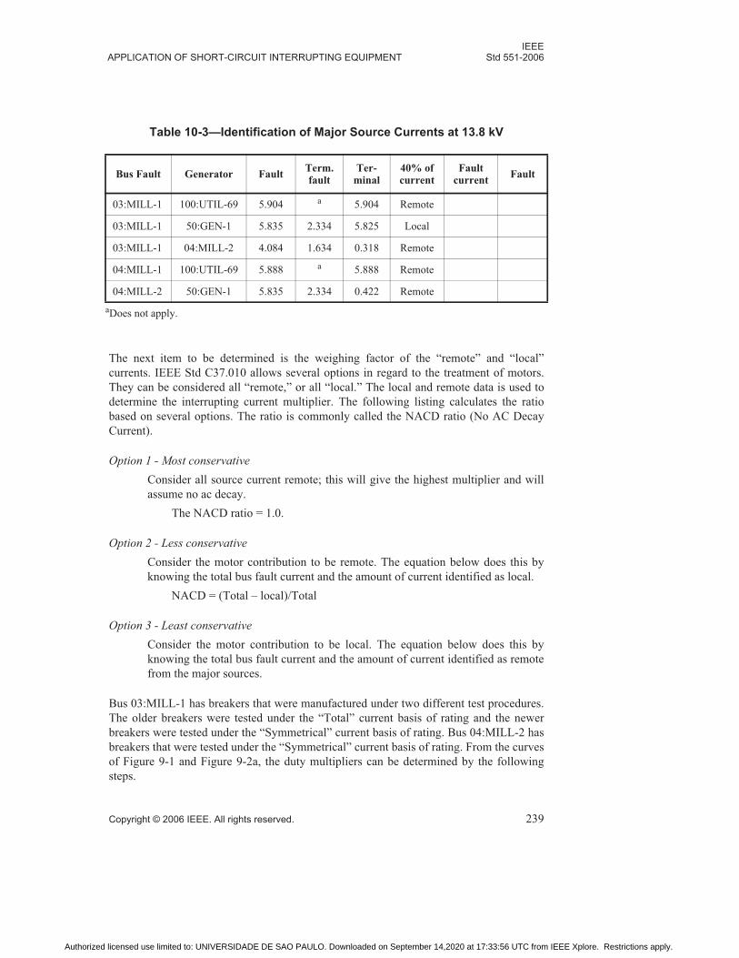
IEEEAPPLICATION OF SHORT-CIRCUIT INTERRUPTING EQUIPMENT Std 551-2006
Copyright © 2006 IEEE. All rights reserved. 239
The next item to be determined is the weighing factor of the “remote” and “local”
currents. IEEE Std C37.010 allows several options in regard to the treatment of motors.
They can be considered all “remote,” or all “local.” The local and remote data is used to
determine the interrupting current multiplier. The following listing calculates the ratio
based on several options. The ratio is commonly called the NACD ratio (No AC Decay
Current).
Option 1 - Most conservativeConsider all source current remote; this will give the highest multiplier and will
assume no ac decay.
The NACD ratio = 1.0.
Option 2 - Less conservativeConsider the motor contribution to be remote. The equation below does this by
knowing the total bus fault current and the amount of current identified as local.
NACD = (Total – local)/Total
Option 3 - Least conservativeConsider the motor contribution to be local. The equation below does this by
knowing the total bus fault current and the amount of current identified as remote
from the major sources.
Bus 03:MILL-1 has breakers that were manufactured under two different test procedures.
The older breakers were tested under the “Total” current basis of rating and the newer
breakers were tested under the “Symmetrical” current basis of rating. Bus 04:MILL-2 has
breakers that were tested under the “Symmetrical” current basis of rating. From the curves
of Figure 9-1 and Figure 9-2a, the duty multipliers can be determined by the following
steps.
Table 10-3—Identification of Major Source Currents at 13.8 kV
Bus Fault Generator FaultTerm. fault
Ter-minal
40% of current
Fault current
Fault
03:MILL-1 100:UTIL-69 5.904 a
aDoes not apply.
5.904 Remote
03:MILL-1 50:GEN-1 5.835 2.334 5.825 Local
03:MILL-1 04:MILL-2 4.084 1.634 0.318 Remote
04:MILL-1 100:UTIL-69 5.888 a 5.888 Remote
04:MILL-2 50:GEN-1 5.835 2.334 0.422 Remote
Authorized licensed use limited to: UNIVERSIDADE DE SAO PAULO. Downloaded on September 14,2020 at 17:33:56 UTC from IEEE Xplore. Restrictions apply.

IEEEAPPLICATION OF SHORT-CIRCUIT INTERRUPTING EQUIPMENT Std 551-2006
Copyright © 2006 IEEE. All rights reserved. 240
Step 1—Determine the Total current multipliers from the REMOTE curves of Figure 9-1
based on the fault point X/R ratio. These multipliers can be taken from the curves or
calculated from the following equation:
(1 + 2 × ε–4πC/(X/R)))1/2
Note that the breakers on bus 04:MILL-2 have an asymmetrical rating factor or 'S' factor
of 1.2. This means that the 5-cycle interrupting time breaker has a contact parting time of
two cycles rather than three cycles normally associated with 5-cycle breakers. For the
breakers rated on a symmetrical current basis divide the multiplier by the breaker “S”
factor (1.1 for bus 03:MILL-1 and 1.2 for bus 04:MILL-2). For the symmetrically rated
breakers this multiplier could have been read directly from Figure 9-2a.
Step 2—Determine the Local current multipliers from the LOCAL curves of Figure 9-1a
and Figure 9-2a based on the fault point X/R ratio. These points can be taken from the
curves or calculated from the empirical equations given in Chapter 9.
Step 3—The final step is to adjust the multipliers based on the NACD ratio. Ratios of 1.0
or 0.0 can use the multipliers directly. The duty multiplier is:
[(Remote Multiplier – Local Multiplier) × NACD Ratio + Local Multiplier]
Table 10-4—Identification of local and remote currents at 13.8 kV—
NACD = remote/total
Total Local Remote NACD ratio
Bus faultFault
currentCurrent Current Option #1 Option #2 Option #3
03:MILL-1 12.902 5.825 6.222 1.000 0.5485 0.4823
04:MILL-2 12.407 4.084 6.310 1.000 0.6708 0.5086
NOTE—Motor contribution not included.
Authorized licensed use limited to: UNIVERSIDADE DE SAO PAULO. Downloaded on September 14,2020 at 17:33:56 UTC from IEEE Xplore. Restrictions apply.

IEEEAPPLICATION OF SHORT-CIRCUIT INTERRUPTING EQUIPMENT Std 551-2006
Copyright © 2006 IEEE. All rights reserved. 241
The breaker ratings at 13.8 kV vary a little depending on the nameplate data even through
they are all the same class of breaker. The AM-13.8-500-3 is the total current rated
breaker and has a constant MVA rating between the rated maximum voltage and the
voltage that results in the maximum interrupting kA (11.5 kV). Applying the breaker at
voltages lower than 11.5 kV, the breaker is a constant current interrupting device. The
breaker interrupting rating at 13.8 kV is shown in Equation (10.3):
500 MVA / 13.8 kV / √3 = 20.9 kA (10.3)
Table 10-5—Local and remote multipliers for buses
03:MILL-1 and 04:MILL-2
Bus Breaker Test stan-dard
Con-tact part time
“S” factor
Fault X/R
Remote mult.
Local mult.
Figure
03:MILL-1 AM-13.8-500-3
Total 4 Cy 1.0 17.92 1.059 0.972 9-1a,1b
03:MILL-1 VB-13.8-500-1
Sym 3 Cy 1.1 17.92 1.115a 1.044a
aDividing these multipliers by “S” will obtain Figure 9-2a and Figure 9-2b.
9-1a,1b
04:MILL-2 15-HK-500
Sym 2 Cy 1.2 22.73 1.289a 1.217a 9-1a,1b
03:MILL-1 AM-13.8-500-3
Total 4 Cy 1.0 17.92 1.059 0.972 9-1a,1b
Table 10-6—Duty current multipliers for buses 03:MILL-1 and 04:MILL-2
Test Fault Final multiplier Duty currentRa-ting
BusStan-dard
Sym kA
Option 1
Option 2
Option 3
Option 1
Option 2
Option 3
kA
03:MILL-1 Total 12.902 1.059 1.020 1.014 13.66 13.16 13.08 20.9
03:MILL-1 Sym 12.902 1.014 1.000a
aIf the final multiplier is less than 1.0 use 1.0.
1.000a 13.08 12.90 12.90 19.6
04:MILL-2 Sym 12.407 1.074 1.054 1.044 13.33 13.08 12.96 21.0
Authorized licensed use limited to: UNIVERSIDADE DE SAO PAULO. Downloaded on September 14,2020 at 17:33:56 UTC from IEEE Xplore. Restrictions apply.

IEEEStd 551-2006 CHAPTER 10
242 Copyright © 2006 IEEE. All rights reserved.
The AM-13.8-500-4 and 15-HK-500 are symmetrical current rated breakers and the
interrupting current is calculated by:
The interrupting capability cannot exceed:
Rated short-circuit current × Voltage range factor
or
First cycle (close and latch)/voltage range factor.
The values should be the same when rounded off.
Breaker VB-13.8-500-1 interrupting rating at 13.8 kV is:
15.0 × 18 / 13.8 = 19.6 kA
The current does not exceed 18 × 1.3 = 23.4 kA breaker maximum interrupting rating.
Breaker 15-HK-500 interrupting rating is:
15.0 × 19.3 / 13.8 = 21.0 kA
The current does not exceed 19.3 × 1.3 = 25.0 kA breaker maximum interrupting rating.
In the above example with the 13.8 kV tie breaker open, the breaker duty current is less
than its rating and the breakers are correctly applied. The fault current when the tie breaker
is closed has not been not been examined for proper equipment application in this book.
However, by following the above procedure the reader can verify the breaker application
when the 13.8 kV tie breaker is closed. From inspection of the one-line diagram and the
above results, the bus duty when the 13.8 kV tie is closed will almost double. For this
system, it appears that the tie 13.8 kV breaker cannot be closed unless a transformer or
generator is out of service.
10.9.2 13.8 kV bus disconnect switch
Bus disconnect switch (Bus 09:FDR E) based on standards has a first cycle asymmetry
factor of 1.6 that is equivalent to a fault X/R ratio of 25. The calculated symmetrical fault
current, from Chapter 9, is 13.268 kA @ 13.8KV with a fault point X/R ratio of 9.82. This
results in an asymmetry factor of 1.44 or 19.00 kA asymmetrical duty. Use
Equation (10.2) to determine the asymmetry factor. The disconnect switch has an
asymmetrical withstand rating of 34 kA and an asymmetrical interrupting rating of 19.2
kA. The asymmetrical interrupting rating would be used if the switch had opening times
Rated max voltage
Bus voltage-------------------------------------------------- Rated short circuit current×
Authorized licensed use limited to: UNIVERSIDADE DE SAO PAULO. Downloaded on September 14,2020 at 17:33:56 UTC from IEEE Xplore. Restrictions apply.

IEEEAPPLICATION OF SHORT-CIRCUIT INTERRUPTING EQUIPMENT Std 551-2006
Copyright © 2006 IEEE. All rights reserved. 243
based on instantaneous relaying. This switch is correctly applied for the first cycle and
interrupting time fault duties calculated.
10.9.3 13.8 kV transformer primary fuse
T17 transformer (Bus 05: FDR F) has a primary fuse and based on standards has an
asymmetry factor of 1.55, which is equivalent to a fault X/R ratio of 15. The fuse
nameplate interrupting rating is 20 kA asymmetrical. However, the manufacturer’s
literature states that these fuses are tested at X/R of 20 or an asymmetry factor of 1.57
(rounded to 1.6 in the literature). Also given in the literature are interrupting ratings at
several X/R ratios less than 20. For this fuse, these ratings are:
X/R = 20 symmetrical interrupting 12.5 kA
X/R = 15 symmetrical interrupting 12.5 kA
X/R = 10 symmetrical interrupting 13.7 kA
X/R = 5 symmetrical interrupting 16.0 kA
The fault point X/R is 12.58 and therefore the fault duty of 13.548 kA symmetrical is
greater than the fuse rating of 12.5 kA symmetrical. This fuse is not correctly applied for
the fault duties calculated and should be replaced with a fuse with a higher interrupting
capability such as an S&C SM-5 fuse, which has a rating of 25 kA symmetrical at an X/Rof 15.
10.9.4 480 V load center
The secondary of load center 28:T10 SEC has three different types of breakers; the main
without an instantaneous trip and high continuous current rating, the motor control center
breaker without an instantaneous trip and lower continuous current rating, and the lighting
panel feeder with a fused breaker with an instantaneous trip and the lowest continuous
current rating. Calculated duties for these devices are listed in Table 10-7.
These breaker are power circuit breaker types and have a test X/R ratio of 6.59 for the non-
fused breaker and 4.9 for the fused breaker. Since the first cycle fault point X/R of 6.55 is
greater than 4.9 required for the fused breaker a current modification may be required. No
modification of the current is needed for the unfused breakers because the breaker test X/Rratio is greater than the fault point X/R ratio. The first cycle breaker duty is 34.56 × 1.0 =
34.56 kA. For the fused breaker, the multiplier is:
First cycle multiplier = Ipeak at fault point X/R/Ipeak at test X/R = 1.061
The peak current multiplier is from the equations that follow.
τ 0.49 0.1ε X R⁄( ) 3⁄–( )–=
Authorized licensed use limited to: UNIVERSIDADE DE SAO PAULO. Downloaded on September 14,2020 at 17:33:56 UTC from IEEE Xplore. Restrictions apply.

IEEEStd 551-2006 CHAPTER 10
244 Copyright © 2006 IEEE. All rights reserved.
10.9.5 480 V motor control center
The motor control center (Bus 33:T10MCC) has molded case breakers with a rating
greater than 20 kA, therefore the test X/R is 4.9 or greater. The motor control center fault
current is 31.87 kA at an X/R of 4.35. No fault current to duty correction is necessary
because of the low X/R ratio. The motor control center has 100 ampere HFD breakers
rated 65 kA interrupting and 60 ampere LC breaker rated 30 kA interrupting. The HFD
breaker is correctly applied and LC breaker is placed in a situation where it is required to
interrupt more current than its rating and has to be replaced with a breaker of higher
interrupting capability. The bus bracing is 42 kA symmetrical and greater than the bus
duty of 31.87 kA.
10.9.6 480 V lighting panelboard
The lighting panelboard (Bus 41:LGTS) has molded case breakers with a rating greater
than 20 kA, therefore the test X/R is 4.9 or greater. The panelboard fault X/R is 4.2 and no
fault current correction is necessary for the breaker duty. Note that the fault current is
32.05 kA on breakers rated 30 kA; the series rating of the class L fuse located on the
480 V load center feeder breaker in combination with the LC breaker has a combined
rating of 100 kA making this a correct application.
10.9.7 Cables
A check on the cables shows that the smallest cable is 250 kcmil and the highest fault that
can occur on the cable is from bus 04: MILL-2. From the Chapter 9 study results, the rms
current is initially 22.03 kA (first cycle rms asymmetrical) and decays to 12.407 kA
(interrupting time symmetrical). If the cable insulation is polyethylene rated 75 ºC, then
the cable can withstand 20 kA for 0.45 seconds and 15 kA for 0.7 seconds.
Table 10-7—Duty current for low-voltage breakers on bus 28:T10 SEC
Test FaultFirst cycle
Short time
Breaker kA rating
Breaker Type X/R X/R kA dutya
aMain breaker given as breaker duty, feeders given as bus duty.
kA duty
1st cyShort time
Main PCB 6.59 6.55 28.68 29.73b
bBreakers without instantaneous trips, short-time rating apply.
85 65b
MCC feeder PCB 6.59 6.55 34.56 29.73b 65 50b
Lighting Fused PCB
4.9 6.55 36.67 29.73 200 -
Ipeak 2 1 ε 2∗πτ X R⁄( )⁄–( )+( )× =
Authorized licensed use limited to: UNIVERSIDADE DE SAO PAULO. Downloaded on September 14,2020 at 17:33:56 UTC from IEEE Xplore. Restrictions apply.

IEEEAPPLICATION OF SHORT-CIRCUIT INTERRUPTING EQUIPMENT Std 551-2006
Copyright © 2006 IEEE. All rights reserved. 245
The times indicate that the cable will not be thermally damaged for faults that are cleared
in instantaneous or with one time step (0.35–0.40 seconds) of relaying.
Some of the pieces of equipment used in the above example are applied close to their
ratings. Closing the 13.8 kV tie breaker would in some cases result in the fault duties
being greater than the equipment withstand or interrupting ratings.
10.10 Equipment ground fault duty calculations
The 13.8 kV system given has a low ground fault current because of the 400 A, 20 ohm
resistors on the generator and transformer neutrals. The ground fault current is
approximately 800 amperes and significantly lower than the breaker interrupting rating so
the ground fault duty is not a concern.
For purposes of illustration, lets assume that bus 03:MILL-1 has a 13.8 kV ground fault
current of 23 kA at an X/R of 10 and all from remote sources. The ANSI standard allows
the breaker ground current interrupting rating to be 15% greater than the phase current
provided the maximum current rating of the breaker is not exceeded. Table 10-8 provides
the breaker rating and duty comparison.
The AM-13.8-500 breaker is correctly applied while the VB-13.8-500 is subject to ground
fault current over its rating.
10.11 Capacitor switching
Breakers used for capacitor switching must be able to withstand the short-circuit duties
between the breaker and capacitor and the transient currents that come from the capacitor
when the fault is on the source side of the breaker. If the size of the load capacitor bank is
equal to or less than the maximum capacitor size allowed by the manufacturer on its
breaker, then the breaker can handle the capacitor current to a fault on the source side of
the breaker. The inrush current when energizing a capacitor is approximately the same as
the current when de-energizing a capacitor bank into a fault. In one case, the source
voltage is known and the capacitor voltage is a zero; in the second case, the internal
Table 10-8—Calculated single-line-to-ground fault duties compared with
breaker ratings
BreakerSym kA
FaultDuty mult.
Duty kA
Phase kA
rating
Gnd. kA
ratingBreaker
AM-13.8-500-3 23.0 1.00 23.0 20.9 24.0 AM-13.8-500-3
VB-13.8-500-1 23.0 1.00 23.0 19.6 22.5 VB-13.8-500-1
Authorized licensed use limited to: UNIVERSIDADE DE SAO PAULO. Downloaded on September 14,2020 at 17:33:56 UTC from IEEE Xplore. Restrictions apply.

IEEEStd 551-2006 CHAPTER 10
246 Copyright © 2006 IEEE. All rights reserved.
voltage of the capacitor is known and the bus voltage is zero. If 1.0 per-unit voltage is
used for either source voltages then the currents are the same. ANSI C37.012-1979 covers
capacitor switching in some detail. Chapter 7 provides summary of capacitor current
considerations.
10.12 Normative references
The following referenced documents are indispensable for the application of this
document. For dated references, only the edition cited applies. For undated references, the
latest edition of the referenced document (including any amendments or corrigenda)
applies.
ANSI C37.06-1997, American National Standard for Switchgear—AC High-Voltage
Circuit Breakers Rated on a Symmetrical Current Basis—Preferred Ratings and Related
Required Capabilities.2
ANSI C37.32-1996, American National Standard for Switchgear-High-Voltage Air
Switches, Bus Supports, and Switch Accessories-Schedules of Preferred Ratings,
Manufacturing Specifications, and Application Guide.
ANSI C37.42-1996, American National Standard Specification for High-Voltage
Expulsion Type Distribution Class Fuses, Cutouts, Fuse Disconnecting Switches and Fuse
Links.
ANSI C37.43-1969, Test Code for High-Voltage Air Switches.3
ANSI C37.44-1981 (Reaff 1992), American National Standard Specifications for
Distribution Oil Cutouts and Fuse Links.
ANSI C37.45-1981 (Reaff 1992), American National Standard Specifications for
Distribution Enclosed Single-Pole Air Switches.
ANSI C37.46-2000, American National Standard for High-Voltage Expulsion and
Current Limiting Type Power Class Fuses and Fuse Disconnecting Switches.
ANSI C37.50-1989, American National Standard for Low-Voltage AC Power Circuit
Breakers Used on Enclosures—Test Procedures.
ANSI C97.1-1972 (R1978), Low-Voltage Cartridge Fuses 600 Volts or Less.4
2ANSI publications are available from the Sales Department, American National Standards Institute, 25 West 43rd Street, 4th Floor, New York, NY 10036, USA (http://www.ansi.org/).3ANSI C37.43-1969 has been withdrawn; however, copies can be obtained from the Sales Department, Ameri-can National Standards Institute, 25 West 43rd Street, 4th Floor, New York, NY 10036, USA (http://www.ansi.org/).4ANSI C97.1-1972 has been withdrawn; however, copies can be obtained from the Sales Department, American National Standards Institute, 25 West 43rd Street, 4th Floor, New York, NY 10036, USA (http://www.ansi.org/).
Authorized licensed use limited to: UNIVERSIDADE DE SAO PAULO. Downloaded on September 14,2020 at 17:33:56 UTC from IEEE Xplore. Restrictions apply.

IEEEAPPLICATION OF SHORT-CIRCUIT INTERRUPTING EQUIPMENT Std 551-2006
Copyright © 2006 IEEE. All rights reserved. 247
IEEE Std C37.04™-1999, IEEE Standard Rating Structure for AC High-Voltage Circuit
Breakers Rated on a Symmetrical Current Basis.5, 6
IEEE Std C37.09™-1999, IEEE Standard Test Procedures for AC High-Voltage Circuit
Breakers Rated on a Symmetrical Current Basis.
IEEE Std C37.010™-1999 (Reaff 2005), IEEE Application Guide for AC High-Voltage
Circuit Breakers Rated on a Symmetrical Current Basis.
IEEE Std C37.012™-1979, IEEE Application Guide for Capacitors Current Switching for
AC High-Voltage Circuit Breakers Rated on a Symmetrical Current Bases.
IEEE Std C37.13™-1990, IEEE Standard for Low-Voltage AC Power Circuit Breakers
used in Enclosures.
IEEE Std C37.30™-1997, American National Standard Definitions and Requirements for
High-Voltage Air Switches, Insulators, and Bus Supports.
IEEE Std C37.34™-1994, IEEE Standard Test Code for High-Voltage Switches.
IEEE Std C37.41™-2000, IEEE Standard Design Tests for Distribution Cutouts and Fuse
Links, Secondary Fuses, Distribution Enclosed Single-Pole Air Switches, Power Fuses,
Fuse Disconnecting Switches, and Accessories.
IEEE Std C57.109™-1993, IEEE Guide for Liquid-Immersed Transformer Through-Fault-
Current Duration.
NEMA AB-1-2002, Molded-Case Circuit Breakers and Circuit-Breaker Enclosures.
NEMA FU-1:2002 Standard for Low-voltage Cartridge Fuses.
NFPA 70, 2005 Edition, National Electric Code® (NEC®).7
UL-RCD, Recognized Component Directory.8
UL 489-2002, Molded-Case Circuit Breakers and Circuit-Breaker Enclosures.
5IEEE publications are available from the Institute of Electrical and Electronics Engineers, 445 Hoes Lane, P.O.Box 1331, Piscataway, NJ 08855-1331, USA (http://standards.ieee.org/).6The IEEE standards or products referred to in this clause are trademarks of the Institute of Electrical and Elec-tronics Engineers, Inc.7The NEC is published by the National Fire Protection Association, Batterymarch Park, Quincy, MA 02269,USA (http://www.nfpa.org/). Copies are also available from the Institute of Electrical and Electronics Engineers,445 Hoes Lane, P.O. Box 1331, Piscataway, NJ 08855-1331, USA (http://standards.ieee.org/).8UL standards are available from Global Engineering Documents, 15 Inverness Way East, Englewood, Colorado80112, USA (http://global.ihs.com/).
Authorized licensed use limited to: UNIVERSIDADE DE SAO PAULO. Downloaded on September 14,2020 at 17:33:56 UTC from IEEE Xplore. Restrictions apply.

Authorized licensed use limited to: UNIVERSIDADE DE SAO PAULO. Downloaded on September 14,2020 at 17:33:56 UTC from IEEE Xplore. Restrictions apply.

Copyright © 2006 IEEE. All rights reserved. 249
Chapter 11Unbalanced short-circuit currents
11.1 Introduction
This chapter describes the calculations for unbalanced short-circuit currents that are the
most common on systems. Other system unbalances, such as an open conductor, are not
covered here because they are not a short-circuit condition. References given at the end of
this chapter can be consulted if this type of circuit failure is of interest. Unbalanced faults
are applicable to utility systems, industrial plants, and commercial buildings. In fact, any
three-phase system is subject to unbalanced faults and they occur more often than three-
phase faults. Generally, fault currents associated with single line-to-ground faults are
lower in magnitude than the currents associated with three-phase faults in the same
locations. However, in some instances, single line-to-ground faults can be more severe
than three-phase faults. The conditions that bring about this unusual situation typically
involve the presence of either multiple grounded-wye autotransformers, or multiple three-
winding transformers in which one winding in each transformer is configured in
grounded-wye.
This chapter is limited to the consideration of short-circuit currents that occur under the
following conditions:
1) Short-circuit fault currents that occur in low-voltage ac systems and medium-
voltage ac systems operating at a constant frequency and electrically remote from
any generators
2) For the duration of the short circuit, there is no change in the source driving
voltage or voltages that caused the initial short-circuit current to flow. In addition,
system impedances remain constant
3) The fault impedance is zero and has no current limiting effect
4) Load currents are much smaller than the fault current and are neglected
11.2 Purpose
The objective of this chapter is to give a procedure for the calculation of unbalanced short-
circuit currents on systems. The network can include equipment with decaying ac fault
current sources such as motors and generators. The application and selection of
interrupting equipment based on the calculated fault current are covered in Chapter 10.
The one-line diagram is the same as used in Chapter 4.
The accurate calculation of unbalanced faults is expedited by the use of symmetrical
components, which are covered in Chapter 3. It must be emphasized that symmetrical
components determine fault voltages and fault currents only. The actual line currents that
flow are a combination of fault, load, and circulating currents. The load or circulating
currents are determined in the pre-fault period under pre-fault conditions. The
superposition theorem permits the addition of the fault currents in each branch of the
Authorized licensed use limited to: UNIVERSIDADE DE SAO PAULO. Downloaded on September 14,2020 at 17:33:56 UTC from IEEE Xplore. Restrictions apply.

IEEEStd 551-2006 CHAPTER 11
250 Copyright © 2006 IEEE. All rights reserved.
network to the pre-fault current. In general, load currents are relatively small with respect
to fault currents and often can be neglected.
11.3 ANSI guidelines
For equipment rating purposes, IEEE Std C37.010™-19991 and IEEE Std C37.13™-1990
basically focus on the maximum fault current magnitudes, which are the result of three-
phase faults. Limited amount of attention is given to unsymmetrical faults because the
interrupting duty is reduced for these types of faults. IEEE Std C37.010 does allow the
line-to-ground interrupting current magnitudes to be 15% greater than a three-phase fault
provided it does not exceed the maximum current rating of the breaker. As with three-
phase faults, a first cycle and interrupting time calculation can be made with the
appropriate change in machine impedances. Because the negative and zero sequence
impedances do not change significantly, the line-to-ground fault current magnitudes vary
less between first cycle and interrupting time currents as compared to the three-phase
currents.
The machine positive sequence impedances used in this chapter will be based on
interrupting and first cycle impedances as given in IEEE Std C37.010-1999. The
representation of synchronous machines by a varying impedance is easily adapted to other
analytical techniques, such as IEC 909.
IEEE Std C37.010 includes three other specifications to be used when calculating fault
currents. These are as follows:
1) The pre-fault bus voltage is 1.0 p.u.
2) Separate resistance and reactance networks are to be used to determine the fault
point X/R ratio. This X/R ratio is to be used to calculate the total asymmetrical
fault current
3) Load currents are much smaller than the fault current and neglected
In this chapter, the symmetrical ac component of the short-circuit current varies based on
the time after the fault. For the purpose of simplicity and conservatism, ANSI has
recommended the following simplified procedure for determining the X/R ratio to be
applied for a particular fault. The system impedance diagram is converted to a separate
resistance (R) diagram and a separate reactance (X) diagram. The resistance and reactance
diagrams are then reduced to a simple resistance (R) and a reactance (X) value at the fault
point. These values are then used to determine the system X/R for a particular fault. The
X/R value in turn determines the system dc time constant and consequently the rate of
decay of the transient dc fault current. By treating the separate R and X as a complex
impedance a close conservative approximation (usually within 0.5% for X/R > 1) to the
true current can be obtained. For simplicity, this method will be used in the sample
calculations.
1Information on normative references can be found in 11.8.
Authorized licensed use limited to: UNIVERSIDADE DE SAO PAULO. Downloaded on September 14,2020 at 17:33:56 UTC from IEEE Xplore. Restrictions apply.

IEEEUNBALANCED SHORT-CIRCUIT CURRENTS Std 551-2006
Copyright © 2006 IEEE. All rights reserved. 251
11.4 Procedure
Some of the most important items in an unbalanced fault calculation are the sequence
component one-line diagrams and the connection of the sequence networks for different
types of faults. The negative sequence diagram is basically the positive sequence diagram
with no voltage source(s) and with some impedances of the synchronous machine being
changed. Often the assumption that the negative sequence impedances are the same as the
positive sequence impedances is used. This is a fairly good assumption except for rotating
machines where the negative sequence impedance is constant and the positive sequence
impedance changes with the time period being studied (to account for ac decay). For first
cycle calculations, the negative sequence impedance and positive sequence impedance are
similar in magnitude.
The zero sequence diagram is more complex and the impedances may not be as readily
available. The type of grounding on generators and transformers must be included in the
zero sequence diagrams. Transformer winding configurations, manner of grounding, and
zero sequence impedances are important and have to be correctly represented or the
results will be meaningless.
The steps in performing an unbalanced fault calculation are as follows:
1) Obtain sequence impedances on the apparatus such as generators, motors, and
transformers and circuits such as cables, duct, and lines
2) Convert impedances to a per-unit value on a common VA base, such as 100 MVA
or 10 MVA, if the per-unit system is used for calculation
3) Construct each of the three sequence impedance networks for the electrical system
that is under study
4) Reduce the sequence networks to simplify calculations (as appropriate)
5) Connect the sequence network for the type of fault desired
6) Calculate the sequence currents
7) Calculate the fault and line currents
Figure 11-1 and Table 11-1 provide the positive, negative, and zero sequence diagrams for
the various types of power system equipment. Figure 11-2a, Figure 11-2b, and
Figure 11-2c provide the sequence diagrams for transformers. These diagrams are
important because they define the flow path of ground current in a transformer and the
possible isolation of ground fault currents from one voltage level to the next. Also note
that the construction of the transformer (core or shell design) may affect the sequence
network or zero sequence impedances.
Authorized licensed use limited to: UNIVERSIDADE DE SAO PAULO. Downloaded on September 14,2020 at 17:33:56 UTC from IEEE Xplore. Restrictions apply.

IEEEStd 551-2006 CHAPTER 11
252 Copyright © 2006 IEEE. All rights reserved.
Figure 11-1—Sequence networks for power system equipment
Authorized licensed use limited to: UNIVERSIDADE DE SAO PAULO. Downloaded on September 14,2020 at 17:33:56 UTC from IEEE Xplore. Restrictions apply.

IEEEUNBALANCED SHORT-CIRCUIT CURRENTS Std 551-2006
Copyright © 2006 IEEE. All rights reserved. 253
Table 11-1—Equipment sequence impedances
Circuit or apparatus
Positive sequence
Negative sequence
Zero sequence
Remarks
Utilitya R1, X1 R2, X2 R0, X0 Often X2 = X1
Syn. generator
R1, X"d, X'd
R2, X2 R0, X0 Usually grounded through a resistor or transformer
Syn. condenser
R1, X"d, X'd
R2, X2 R0, X0 Neutral may or may not be grounded
Syn. motor R1, X"d, X'd
R2, X2 R0, X0 Neutral seldom grounded
Induction motor
R1, X" R2, X2 R0, X0 Neutral not grounded
Transformer R1, X1 R1, X1 R0, X0 Wye winding usually solidly or impedance grounded
Figure 11-1—Sequence networks for power system equipment (continued)
Authorized licensed use limited to: UNIVERSIDADE DE SAO PAULO. Downloaded on September 14,2020 at 17:33:56 UTC from IEEE Xplore. Restrictions apply.

IEEEStd 551-2006 CHAPTER 11
254 Copyright © 2006 IEEE. All rights reserved.
Figure 11-2a shows a diagram that will be used to explain the sequence networks for
transformers. The information will be presented in tabular form in Table 11-2 for given
connections to obtain the sequence networks. The table will show how major nodes will
be connected.
As an example, Figure 11-2b shows the positive and zero sequence connections for a
three-phase transformer with the HV (h) winding connected in delta and the LV (x)
winding connected in grounded wye (through impedance Zg).
Auto-transformer
R1, X1 R1, X1 R0, X0 Usually solidly grounded
Reactor R1, X1 R1, X1 R1, X1
Neutral resistor
— — 3R1
Neutral reactor
— — 3X1
Cable R1, X1 R1, X1 R0, X0
Overhead lines
R1, X1 R1, X1 R0, X0
Busway R1, X1 R1, X1 R0, X0
aNote that the utility system representation will typically be a Thevenin equivalent obtained by areduction of the utility system at the fault point. The equivalent impedance is often a worst-casevalue (to give the highest fault current) and will not be modified for ac decay.
Table 11-1—Equipment sequence impedances (continued)
Circuit or apparatus
Positive sequence
Negative sequence
Zero sequence
Remarks
Figure 11-2a—Sequence networks for transformers
ZH ZXh hh hhh xxxxxx
R (reference)
Authorized licensed use limited to: UNIVERSIDADE DE SAO PAULO. Downloaded on September 14,2020 at 17:33:56 UTC from IEEE Xplore. Restrictions apply.

IEEEUNBALANCED SHORT-CIRCUIT CURRENTS Std 551-2006
Copyright © 2006 IEEE. All rights reserved. 255
Table 11-2—Connection specifications for Figure 11-2a
Transformer connectionsPositive or negative
sequenceZero sequence
Winding H Winding L Winding H Winding L Winding H Winding L
Delta Wye Short hh to hhh
Short xx to xxx
Short hhh to R Open xxx to xx
Delta Solidly grounded wye
Short hh to hhh
Short xx to xxx
Short hhh to R Short xx to xxx
Delta Wye (grounded through Zgnd)
Short hh to hhh
Short xx to xxx
Short hhh to R Connect xx to xxx through 3Zgnd
Delta Delta Short hh to hhh
Short xx to xxx
Short hhh to R Short xxx to R
Wye Wye Short hh to hhh
Short xx to xxx
Open hhh to hh Open xxx to xx
Wye Solidly grounded wye
Short hh to hhh
Short xx to xxx
Open hhh to hh Short xx to xxx
Wye Wye (grounded through Zgnd)
Short hh to hhh
Short xx to xxx
Open hhh to hh Connect xx to xxx through 3Zgnd
Solidly grounded wye
Solidly grounded wye
Short hh to hhh
Short xx to xxx
Short hh to hhh Short xx to xxx
Solidly grounded wye
Wye (grounded through Zgnd)
Short hh to hhh
Short xx to xxx
Short hh to hhh Connect xx to xxx through 3Zgnd
Wye (grounded through Zgnd)
Wye (grounded through Zgnd)
Short hh to hhh
Short xx to xxx
Connect hh to hhh through 3Zgnd
Connect xx to xxx through 3Zgnd
Authorized licensed use limited to: UNIVERSIDADE DE SAO PAULO. Downloaded on September 14,2020 at 17:33:56 UTC from IEEE Xplore. Restrictions apply.

IEEEStd 551-2006 CHAPTER 11
256 Copyright © 2006 IEEE. All rights reserved.
Figure 11-2c shows the diagram used to explain the sequence networks for three-winding
(three-phase) transformers. The connections are based upon the information given in
Table 11-2. For example, assume the following transformer connections: a delta (primary
winding, h) to solidly grounded wye (secondary winding, x) connection with the tertiary
winding (t) connected in delta. The positive and negative sequence network would consist
of shorting “hh to hhh,” “xxx to xx,” and “ttt to tt.” The zero sequence network would
have the “h” and “t” windings with “hh to hhh” and “tt to ttt” open and with “hhh” and
“ttt” shorted to reference. The secondary would have “xxx” connected to “xx” through a
zero impedance branch.
Figure 11-2b—Example sequence networks for delta to impedance
grounded wye transformer connection
ZH ZX
R (reference)
ZH ZX
R (reference)
Positive
sequence
circuit
Zero
sequence
circuit
3*Zg
HV
winding
LV
winding
HV
winding
LV
winding
Figure 11-2c—Sequence networks for transformers with tertiary windings
ZH ZXh hh hhh xxxxxx
R (reference)
ZTtttttt
Authorized licensed use limited to: UNIVERSIDADE DE SAO PAULO. Downloaded on September 14,2020 at 17:33:56 UTC from IEEE Xplore. Restrictions apply.
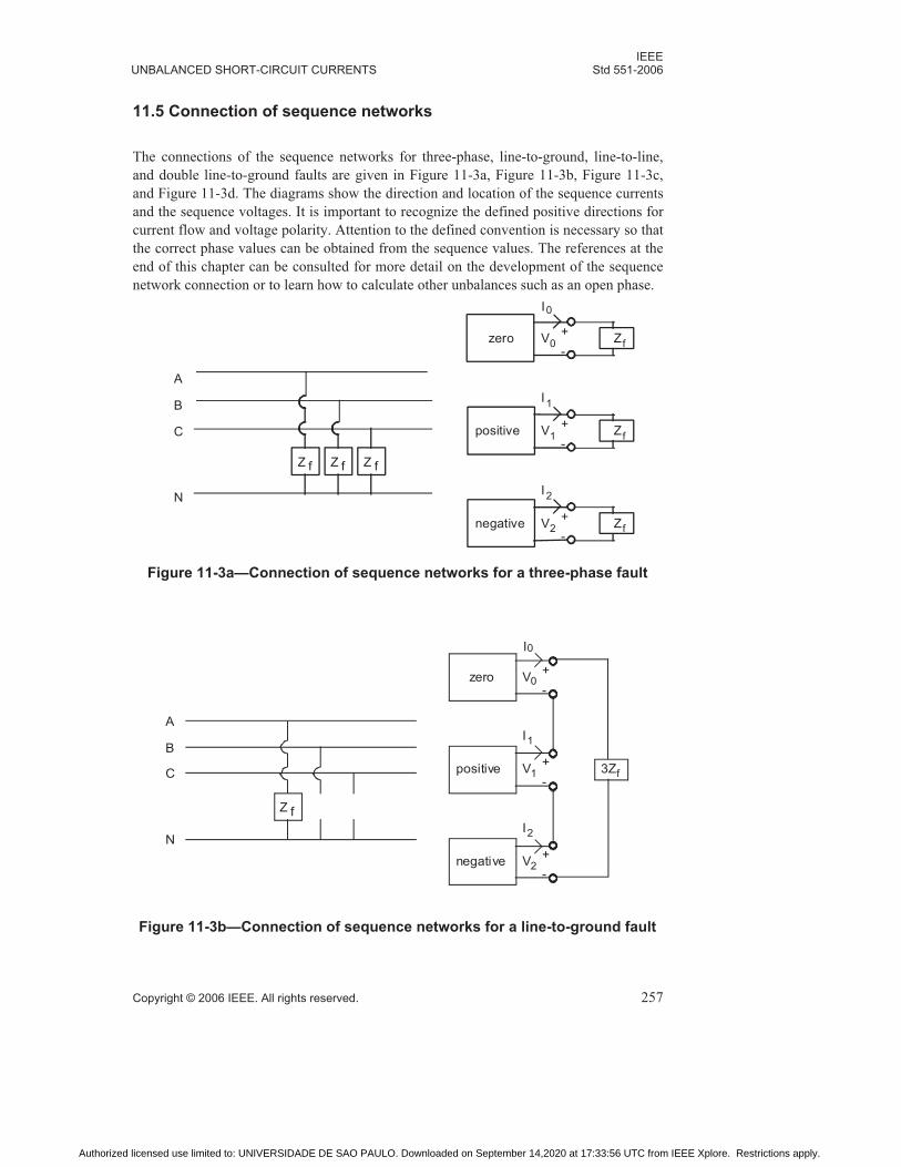
IEEEUNBALANCED SHORT-CIRCUIT CURRENTS Std 551-2006
Copyright © 2006 IEEE. All rights reserved. 257
11.5 Connection of sequence networks
The connections of the sequence networks for three-phase, line-to-ground, line-to-line,
and double line-to-ground faults are given in Figure 11-3a, Figure 11-3b, Figure 11-3c,
and Figure 11-3d. The diagrams show the direction and location of the sequence currents
and the sequence voltages. It is important to recognize the defined positive directions for
current flow and voltage polarity. Attention to the defined convention is necessary so that
the correct phase values can be obtained from the sequence values. The references at the
end of this chapter can be consulted for more detail on the development of the sequence
network connection or to learn how to calculate other unbalances such as an open phase.
Figure 11-3a—Connection of sequence networks for a three-phase fault
zero
positive
negative
+
-
V 0
I 0
+
-
V 1
I 1
+
-
V 2
I 2
Z f
Z f
Z f
A
B
C
N
Z f Z f Z f
Figure 11-3b—Connection of sequence networks for a line-to-ground fault
A
B
C
N
Z f
zero
positive
negative
+
-V0
0
+
-V1
I1
+
-V2
I2
3Zf
I
Authorized licensed use limited to: UNIVERSIDADE DE SAO PAULO. Downloaded on September 14,2020 at 17:33:56 UTC from IEEE Xplore. Restrictions apply.

IEEEStd 551-2006 CHAPTER 11
258 Copyright © 2006 IEEE. All rights reserved.
11.6 Sample calculations
For illustration purposes, a first cycle line-to-ground and a line-to-line fault will be
calculated at the primary and secondary of transformer T-14. The circuit impedances and
equivalents from the three-phase fault conditions in Chapter 9 will be used to reduce the
amount of network reduction required for the sample calculations. The condition
represented has all motors and generators in service. Figure 11-4 shows the positive and
zero sequence networks for feeder M. In this case, the positive and negative sequence
impedances will be assumed to be equal. Because the main bus has a generator connected
Figure 11-3c—Connection of sequence networks for a line-to-line fault
A
B
C
N
Z f
zero
positive
negative
+
-V0
I0
+
-V1
I1
+
-V2
I2Zf
Figure 11-3d—Connection of sequence networks for a double
line-to-ground fault
A
B
C
N
Z f
zero
positive
negative
+
-V0
I0
+
-V1
I1
+
-V2
I2
3Zf
Authorized licensed use limited to: UNIVERSIDADE DE SAO PAULO. Downloaded on September 14,2020 at 17:33:56 UTC from IEEE Xplore. Restrictions apply.
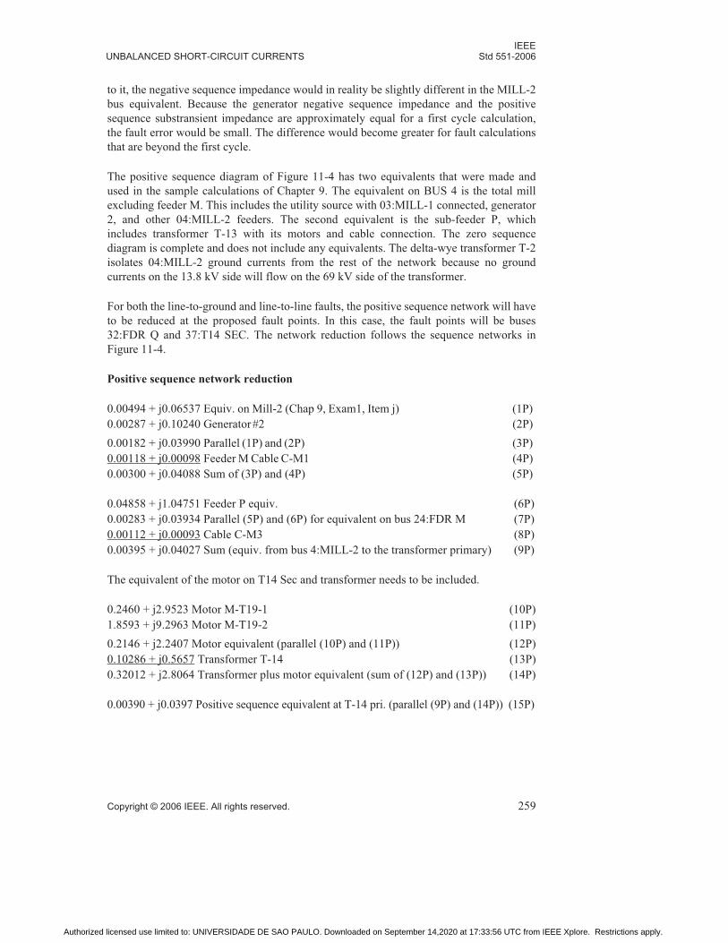
IEEEUNBALANCED SHORT-CIRCUIT CURRENTS Std 551-2006
Copyright © 2006 IEEE. All rights reserved. 259
to it, the negative sequence impedance would in reality be slightly different in the MILL-2
bus equivalent. Because the generator negative sequence impedance and the positive
sequence substransient impedance are approximately equal for a first cycle calculation,
the fault error would be small. The difference would become greater for fault calculations
that are beyond the first cycle.
The positive sequence diagram of Figure 11-4 has two equivalents that were made and
used in the sample calculations of Chapter 9. The equivalent on BUS 4 is the total mill
excluding feeder M. This includes the utility source with 03:MILL-1 connected, generator
2, and other 04:MILL-2 feeders. The second equivalent is the sub-feeder P, which
includes transformer T-13 with its motors and cable connection. The zero sequence
diagram is complete and does not include any equivalents. The delta-wye transformer T-2
isolates 04:MILL-2 ground currents from the rest of the network because no ground
currents on the 13.8 kV side will flow on the 69 kV side of the transformer.
For both the line-to-ground and line-to-line faults, the positive sequence network will have
to be reduced at the proposed fault points. In this case, the fault points will be buses
32:FDR Q and 37:T14 SEC. The network reduction follows the sequence networks in
Figure 11-4.
Positive sequence network reduction
0.00494 + j0.06537 Equiv. on Mill-2 (Chap 9, Exam1, Item j) (1P)
0.00287 + j0.10240 Generator #2 (2P)
0.00182 + j0.03990 Parallel (1P) and (2P) (3P)
0.00118 + j0.00098 Feeder M Cable C-M1 (4P)
0.00300 + j0.04088 Sum of (3P) and (4P) (5P)
0.04858 + j1.04751 Feeder P equiv. (6P)
0.00283 + j0.03934 Parallel (5P) and (6P) for equivalent on bus 24:FDR M (7P)
0.00112 + j0.00093 Cable C-M3 (8P)
0.00395 + j0.04027 Sum (equiv. from bus 4:MILL-2 to the transformer primary) (9P)
The equivalent of the motor on T14 Sec and transformer needs to be included.
0.2460 + j2.9523 Motor M-T19-1 (10P)
1.8593 + j9.2963 Motor M-T19-2 (11P)
0.2146 + j2.2407 Motor equivalent (parallel (10P) and (11P)) (12P)
0.10286 + j0.5657 Transformer T-14 (13P)
0.32012 + j2.8064 Transformer plus motor equivalent (sum of (12P) and (13P)) (14P)
0.00390 + j0.0397 Positive sequence equivalent at T-14 pri. (parallel (9P) and (14P)) (15P)
Authorized licensed use limited to: UNIVERSIDADE DE SAO PAULO. Downloaded on September 14,2020 at 17:33:56 UTC from IEEE Xplore. Restrictions apply.

IEEEStd 551-2006 CHAPTER 11
260 Copyright © 2006 IEEE. All rights reserved.
Fig
ure
11
-4—
On
e-l
ine d
iag
ram
an
d s
eq
ue
nce
netw
ork
fo
r fe
ed
er
M
Authorized licensed use limited to: UNIVERSIDADE DE SAO PAULO. Downloaded on September 14,2020 at 17:33:56 UTC from IEEE Xplore. Restrictions apply.

IEEEUNBALANCED SHORT-CIRCUIT CURRENTS Std 551-2006
Copyright © 2006 IEEE. All rights reserved. 261
For the positive sequence equivalent on T-14 secondary, add T-14 transformer impedance
to the equivalent in item (9P) and in parallel with the motor equivalent.
0.00395 + j0.04027 (9P)
0.10286 + j0.56570 Transformer T-14 (13P)
0.10681 + j0.60597 Sum (equivalent from Bus 4:MILL-2 to transformer secondary) (16P)
0.07584 + j0.47749 Total positive sequence on the 480 V Bus 37:T14SEC (17P)
Parallel equivalent of (12P) and (16P)
Zero sequence network reduction
The same network reduction procedure is followed for the zero sequence network
beginning with the ground sources on the incoming transformer T-2 and generator 2. The
zero sequence impedance of the resistor is three times its given value because during a
ground fault, currents in the three phases flow through it (see Figure 11-1). Note that
Resistorpu = 3 × ohm × Base MVA / kV2 = 3 × 20 × 10 / 13.82 = 3.1506.
3.1506 + j0.0000 Grounding resistor on T-2 (1G)
0.0029 + j0.04925 Transformer T-2 (2G)
3.1535 + j0.04925 Sum (1G) and (2G) (3G)
3.1506 + j0.0000 Grounding resistor on GEN-2 (4G)
0.0029 + j0.04925 Generator GEN-2 (5G)
3.1535 + j0.04925 Sum (4G) and (5G) (6G)
The parallel equivalent of the two grounding sources (3G) and (6G) is:
1.57635 + j0.02389 (7G)
0.00236 + j0.00196 Cable C-M1 (8G)
0.00224 + j0.00187 Cable C-M2 (9G)
1.58095 + j0.02772 Sum (7G), (8G), and (9G) (10G)
9999.9 + j99999.9 Equivalent of motors and transformer to 13.8 kV (11G)
The result is the zero sequence equivalent to T-14 primary. Note that the motors and
transformer on sub-feeder P do not enter into the equivalent at bus 24:FDR M because of
the delta primary winding (open circuit for zero sequence) of transformer T-13. The
motors and transformer of T-14 are not included for the same reason.
For this one-line diagram, the equivalent ground source on the secondary of the
transformer is the transformer zero sequence impedance. The motors are not grounded and
do not become part of the zero sequence network.
0.10286 + j0.56573 Transformer T-14 (12G)
9999.9 + j99999.9 Equivalent of motors (13G)
Authorized licensed use limited to: UNIVERSIDADE DE SAO PAULO. Downloaded on September 14,2020 at 17:33:56 UTC from IEEE Xplore. Restrictions apply.

IEEEStd 551-2006 CHAPTER 11
262 Copyright © 2006 IEEE. All rights reserved.
Once the equivalents have been made, the sequence networks can be connected together
for the desired fault type. See Figure 11-3 for the appropriate connections and the
direction of the sequence currents. The positive, negative, and zero sequence networks are
connected in series for the line-to-ground faults as shown in Figure 11-5 and the positive
and negative sequence networks are connected in parallel for the line-to-line fault.
11.6.1 Line-to-ground fault calculation
Calculating a line-to-ground fault on the primary of transformer T-14 requires the
positive, negative, and zero sequence network equivalents at the primary of the
transformer as determined previously. Because in this example the positive and negative
sequence networks will be assumed equal, the equivalent of item (15P) is used. The
equivalent of the zero sequence network is given in (10G). The three sequence networks
are connected in series as shown in Figure 11-3b.
0.00390 + j0.03970 Positive sequence
0.00390 + j0.03970 Negative sequence
1.58095 + j0.02772 Zero sequence
1.58875 + j0.10712 Sum
Figure 11-5—Connection of sequence network for line-to-ground faults
1.0
PU
0.00395 + j0.04027 0.00395 + j0.04027 1.58095 + j0.02772
0.32012 + j2.8064 0.32012 + j2.8064 9999.9 + j99999.9
Positive Negative Zero
13.8 KV
Side
480 V
Side
Impedance diagram for fault on transformer T14 primary
(9P)
(14P)
(9P)
(14P)
(10G)
(11G)
1.0
PU
0.10681 + j0.60597 0.10681 + j0.60597 0.10286 + j0.56573
0.2146 + j2.2407 0.2146+ j2.2407 9999.9 + j99999.9
Positive Negative Zero
Transformer
Side
Motor
Side
Impedance diagram for fault on transformer T14 secondary
(16P)
(12P)
(16P)
(12P)
(12G)
(13G)
Authorized licensed use limited to: UNIVERSIDADE DE SAO PAULO. Downloaded on September 14,2020 at 17:33:56 UTC from IEEE Xplore. Restrictions apply.

IEEEUNBALANCED SHORT-CIRCUIT CURRENTS Std 551-2006
Copyright © 2006 IEEE. All rights reserved. 263
Using Equation (3.16) from Chapter 3, the ground fault current can be calculated. For the
current into the fault, the equation will yield the following 13.8 kV current:
Ia = Ia0 + Ia1 + Ia2
Ib = Ia0 + Ia1
Ic = Ia0 + Ia1
Ia = Ifault = 3I0 = 788.2 A
Ib = 0
Ic = 0
Often on resistance grounded systems, a rigorous line-to-ground fault calculation is not
made. The sum of the current rating of each resistor is used. For the 20 ohm resistors in the
above example, the maximum fault current would be 13 800/(1.732 × 20) = 398.4 amperes
per resistor or 796.8 amperes total. This is only 1% higher than the 788.2 amperes
calculated by the more rigorous method and well within the tolerance of any relay setting.
I0EZ---
1
1.58875 j0.10712+----------------------------------------------- 0.6280@ 3.86° p.u.–= = =
I00.62801 10×
13.8 1000 1.732××------------------------------------------------ 262.7A= =
240 Ia2+ 120∠∠
120 Ia2+ 240∠∠
Authorized licensed use limited to: UNIVERSIDADE DE SAO PAULO. Downloaded on September 14,2020 at 17:33:56 UTC from IEEE Xplore. Restrictions apply.

IEEEStd 551-2006 CHAPTER 11
264 Copyright © 2006 IEEE. All rights reserved.
Figure 11-6 shows the division of the sequence current in each of the networks for a fault
on the transformer primary. The division was determined by the equivalent sequence
impedance as given in Figure 11-5.
Using Equation (3.16), the line currents on each side of the transformer can be calculated.
The phase A, B, and C currents on the primary side of the transformer are determined by
the sequence currents shown on the 13.8 kV side of the transformer.
The currents on the 480 V side are calculated by the same equations. However, because
the delta-wye transformer shifts the secondary side by –30º degrees with respect to the
primary, the angle has to be included in the sequence components on the secondary. The
positive sequence current on the secondary has angle 30º subtracted from it, the negative
sequence current on the secondary has angle 30º added to it, and the zero sequence is not
shifted. The calculation of phase values can only take place after these angles have been
introduced in the sequence values. The phase currents are shown in Figure 11-7. Note that
the line-to-ground fault on the transformer primary appears as a line-to-line fault on the
secondary.
Figure 11-6—Division of sequence currents for a line-to-ground fault on
T-14 transformer primary
1.0 PU
Positive Negative Zero
13.8 KV
Side
480 V
Side
262.7∠-3.86°
259.0∠-3.87°
3.7∠-2.97°
259.0∠-3.87°
3.7∠-2.97°
262.7∠-3.86°
0.0
Authorized licensed use limited to: UNIVERSIDADE DE SAO PAULO. Downloaded on September 14,2020 at 17:33:56 UTC from IEEE Xplore. Restrictions apply.

IEEEUNBALANCED SHORT-CIRCUIT CURRENTS Std 551-2006
Copyright © 2006 IEEE. All rights reserved. 265
Calculating a line-to-ground fault on the secondary of transformer T-14 requires the
positive, negative, and zero sequence network equivalents at the secondary of the
transformer as determined previously. In this example the positive and negative sequence
networks will be assumed equal and the equivalent of item (17P) is used. The equivalent
of the zero sequence network is given in 12G.
0.07132 + j0.47698 Positive sequence
0.07132 + j0.47698 Negative sequence
0.10286 + j0.56573 Zero sequence
0.24550 + j1.51969 Sum
Using Equation (3.16) from Chapter 3, the ground fault current can be calculated. For the
current into the, fault the equation will yield the following 480 V current:
Ia = Ifault = 3I0 = 24.523 kA
Ib = 0
Ic = 0
Figure 11-7—Line currents for a line-to-ground fault on
T14 transformer primary
3.7∠-3.16°
3.7∠-3.16°
788.1∠-3.86° 780.7∠-3.87°
0
184.3∠-3.16°
7.4∠-3.16°
184.3∠-3.16°
A
B
C
b
a
c
I0EZ---
1
1.24550 j1.51969+----------------------------------------------- 0.64960 80.8° p.u.–∠= = =
I00.6496 10×
0.48 1000 1.732××------------------------------------------------ 8174 A= =
Authorized licensed use limited to: UNIVERSIDADE DE SAO PAULO. Downloaded on September 14,2020 at 17:33:56 UTC from IEEE Xplore. Restrictions apply.

IEEEStd 551-2006 CHAPTER 11
266 Copyright © 2006 IEEE. All rights reserved.
Figure 11-8 shows the division of the sequence current in each of the networks for a fault
on the transformer secondary. The division was determined by the equivalent sequence
impedance as given in Figure 11-5.
The line current flows on each side of the transformer are shown in Figure 11-9. The line
currents on the primary side of the transformer are calculated using Equation (3.16).
The phase a, b, and c currents on the secondary side of the transformer are determined by
the sequence currents shown on the 480 V side of the transformer. However, because the
delta-wye transformer shifts the primary side by 30º degrees with respect to the secondary,
the angle has to be included in the sequence components on the primary. The positive
sequence current on the primary has angle 30º added to it, the negative sequence current
on the primary has angle 30º subtracted from it, and the zero sequence is not shifted. The
calculation of phase values can only take place after these angles have been introduced in
Figure 11-8—Division of sequence currents for a line-to-ground fault on T14
transformer secondary
1.0
PU
Positive Negative Zero
Transformer
Side
Motor Side
8174∠-80.8°
6422∠-79.8°
1756∠-84.4°
6422∠-79.8°
1756∠-84.4°
8174∠-80.8°
0.0
Figure 11-9—Line currents for a line-to-ground fault on
T14 transformer secondary
0
386.7∠-79.8°
24522∠-80.8° 386.7∠-79.8°
1757∠-84.5°
21017∠-80.2°
1757∠-84.5°
Motors
3514∠-84.5° A
B
C
a
b
c
Authorized licensed use limited to: UNIVERSIDADE DE SAO PAULO. Downloaded on September 14,2020 at 17:33:56 UTC from IEEE Xplore. Restrictions apply.

IEEEUNBALANCED SHORT-CIRCUIT CURRENTS Std 551-2006
Copyright © 2006 IEEE. All rights reserved. 267
the sequence values. The line-to-ground fault on the transformer secondary appears as a
line-to-line fault to the 13.8 kV system.
11.6.2 Line-to-line fault calculation
Calculating a line-to-line fault on the primary of transformer T-14 requires the positive
and negative sequence networks. The zero sequence network is not required. In this
example the positive and negative sequence networks will be assumed equal and the
equivalent of item (15P) is used. Also note in Figure 11-3c that for a line-to-line fault the
negative sequence current is the reverse of the positive sequence current flow.
0.00390 + j0.03970 Positive sequence
0.00390 + j0.03970 Negative sequence
0.00780 + j0.07940 Sum
I2 = I1 = –5244 A
I0 = 0
Using Equation (3.16) from Chapter 3, the phase-to-phase fault current can be calculated.
For the current into the fault, the equation will yield the following:
Ia = 0
Ib = 9083 A
Ic = 9083 A
Often for line-to-line faults, a rigorous calculation is not made. The line-to-line fault
current is 86.6% of the three-phase fault current when the positive and negative sequence
networks are equal.
I0EZ---
1
0.00780 j0.07940+----------------------------------------------- 12.534 84.39° p.u.–∠= = =
I012.534 10×
13.8 1000 1.732××------------------------------------------------ 5244 A= =
Authorized licensed use limited to: UNIVERSIDADE DE SAO PAULO. Downloaded on September 14,2020 at 17:33:56 UTC from IEEE Xplore. Restrictions apply.

IEEEStd 551-2006 CHAPTER 11
268 Copyright © 2006 IEEE. All rights reserved.
Figure 11-10 shows the division of the sequence currents in each of the networks for a
fault on the transformer primary. The division was determined by the equivalent sequence
impedance as given in Figure 11-5.
Using Equation (3.16), the line currents on each side of the transformer can be calculated.
The phase A, B, and C currents on the primary side of the transformer are determined by
the sequence currents shown on the 13.8 kV side of the transformer. The currents on the
480 side are calculated by the same equations. However, because the delta-wye
transformer shifts the secondary side by –30º degrees with respect to the primary, the
angle has to be included in the sequence components on the secondary. The positive
sequence current on the secondary has angle 30º subtracted from it, the negative sequence
current on the secondary has angle 30º added to it, and the zero sequence is not shifted.
The calculation of phase values can only take place after these angles have been
introduced in the sequence values. The phase currents are shown in Figure 11-11.
Figure 11-10—Division of sequence currents for a line-to-line fault on T14
transformer primary
1.0 PU
Positive
13.8 KV
Side
480 V
Side
5244∠-84.4°
5169.9∠-84.3°
74.1∠-83.5°
-5169.9∠-84.3°
Negative
-74.1∠-83.5°
Figure 11-11—Line currents for a line-to-line fault on
T14 transformer primary
8955∠5.7°
8955∠5.7°
9083∠5.6°
0
4238.3∠-1.37°
2141.6∠-1.4°
128.96∠-1.4°
128.96∠-1.4°
2141.6∠-1.4°
A
BC
a
b
c
Authorized licensed use limited to: UNIVERSIDADE DE SAO PAULO. Downloaded on September 14,2020 at 17:33:56 UTC from IEEE Xplore. Restrictions apply.
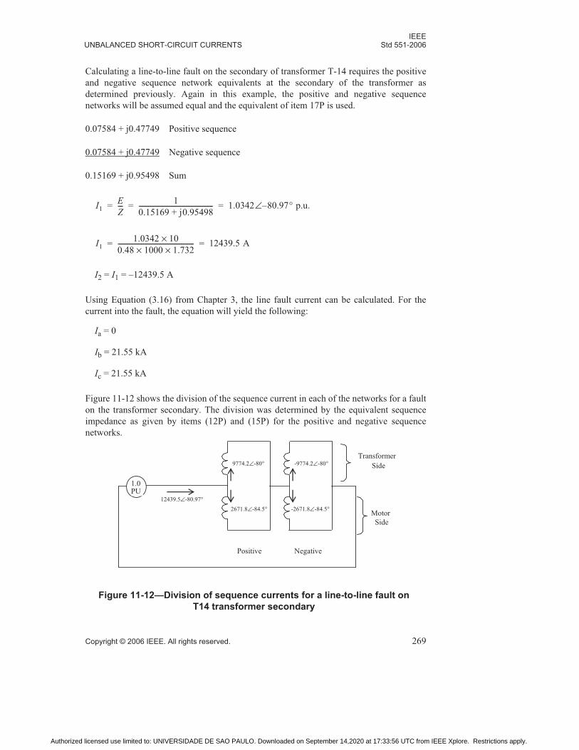
IEEEUNBALANCED SHORT-CIRCUIT CURRENTS Std 551-2006
Copyright © 2006 IEEE. All rights reserved. 269
Calculating a line-to-line fault on the secondary of transformer T-14 requires the positive
and negative sequence network equivalents at the secondary of the transformer as
determined previously. Again in this example, the positive and negative sequence
networks will be assumed equal and the equivalent of item 17P is used.
0.07584 + j0.47749 Positive sequence
0.07584 + j0.47749 Negative sequence
0.15169 + j0.95498 Sum
I2 = I1 = –12439.5 A
Using Equation (3.16) from Chapter 3, the line fault current can be calculated. For the
current into the fault, the equation will yield the following:
Ia = 0
Ib = 21.55 kA
Ic = 21.55 kA
Figure 11-12 shows the division of the sequence current in each of the networks for a fault
on the transformer secondary. The division was determined by the equivalent sequence
impedance as given by items (12P) and (15P) for the positive and negative sequence
networks.
I1EZ---
1
0.15169 j0.95498+----------------------------------------------- 1.0342 80.97° p.u.–∠= = =
I11.0342 10×
0.48 1000 1.732××------------------------------------------------ 12439.5 A= =
Figure 11-12—Division of sequence currents for a line-to-line fault on
T14 transformer secondary
1.0 PU
Positive
Transformer
Side
Motor
Side
12439.5∠-80.97°
9774.2∠-80°
2671.8∠-84.5°
-9774.2∠-80°
Negative
-2671.8∠-84.5°
Authorized licensed use limited to: UNIVERSIDADE DE SAO PAULO. Downloaded on September 14,2020 at 17:33:56 UTC from IEEE Xplore. Restrictions apply.

IEEEStd 551-2006 CHAPTER 11
270 Copyright © 2006 IEEE. All rights reserved.
The line current flows are shown in Figure 11-13. The line currents on the primary side of
the transformer can be calculated using Equation (3.16). The phase a, b, and c currents on
the secondary side of the transformer are determined by the sequence currents. However,
because the delta-wye transformer shifts the primary side by 30º degrees with respect to
the secondary, the angle has to be included in the sequence components on the primary.
The positive sequence current on the primary has angle 30º added to it, the negative
sequence current on the primary has angle 30º subtracted from it, and the zero sequence is
not shifted. The calculation of phase values can only take place after these angles have
been introduced in the sequence values.
11.7 Conclusions
In this chapter, the analytical methods and techniques for calculating unbalanced short-
circuit currents have been introduced. Of primary importance is the concept of
interconnecting sequence networks (in either full or reduced form) to simulate the
unbalanced effects of different fault types. The calculation methods, based on the method
of symmetrical components, have been presented, but it has been shown that such rigorous
calculations are not always necessary. As was discussed, single line-to-ground fault
currents can often be found by considering only the system grounding impedances while
the line-to-line fault currents are typically very nearly equal to 86.6% of the three-phase
fault current values.
Figure 11-13—Division of line currents for a line-to-line fault on
T14 transformer secondary
679.7∠10°
339.8∠10°
16930∠10°
0
Motors 4627.3∠5.5°
339.8∠10° 21546∠9°
4627.3∠5.5°
16930∠10°
A
B
C
a
c
b
Authorized licensed use limited to: UNIVERSIDADE DE SAO PAULO. Downloaded on September 14,2020 at 17:33:56 UTC from IEEE Xplore. Restrictions apply.

IEEEUNBALANCED SHORT-CIRCUIT CURRENTS Std 551-2006
Copyright © 2006 IEEE. All rights reserved. 271
11.8 Normative references
The following referenced documents are indispensable for the application of this
document. For dated references, only the edition cited applies. For undated references, the
latest edition of the referenced document (including any amendments or corrigenda)
applies.
IEC 909, Short-Circuit Current Calculations in Three-Phase A.C. Systems.2
IEEE Std C37.010™-1999, IEEE Application Guide for AC High-Voltage Circuit Break-
ers Rated on a Symmetrical Current Basis.3, 4
IEEE Std C37.13™-1990 (Reaff 1995), IEEE Standard for Low-Voltage AC Power
Circuit Breakers Used on Enclosures.
11.9 Bibliography
[B1] Beeman, Donald, Industrial Power Systems Handbook. McGraw-Hill.
[B2] Brown, Homer E., Solution of Large Networks By Matrix Methods. Wiley Book.
[B3] Calabrese, G. O., Symmetrical Components. The Ronald Press Company, 1959.
[B4] IEEE Std 141™-1993, Electric Power Distribution for Industrial Plants (IEEE RedBook).
[B5] IEEE Std 242™-2001, IEEE Recommended Practice for Protection and Coordination
of Industrial and Commercial Power Systems (IEEE Buff Book).
[B6] Rothe, F. S. An Introduction to Power System Analysis. Wiley Book.
[B7] Wagner, C. F., and R.D. Evans, Symmetrical Components. McGraw-Hill Book
Company, 1933.
[B8] Westinghouse Electrical Transmission & Distribution Reference Book.
2IEC publications are available from the Sales Department of the International Electrotechnical Commission,Case Postale 131, 3, rue de Varembé, CH-1211, Genève 20, Switzerland/Suisse (http://www.iec.ch/). IEC publi-cations are also available in the United States from the Sales Department, American National Standards Institute,11 West 42nd Street, 13th Floor, New York, NY 10036, USA.3IEEE publications are available from the Institute of Electrical and Electronics Engineers, 445 Hoes Lane, P.O.Box 1331, Piscataway, NJ 08855-1331, USA (http://standards.ieee.org/).4The IEEE standards or products referred to in this clause are trademarks of the Institute of Electrical and Elec-tronics Engineers, Inc.
Authorized licensed use limited to: UNIVERSIDADE DE SAO PAULO. Downloaded on September 14,2020 at 17:33:56 UTC from IEEE Xplore. Restrictions apply.

Authorized licensed use limited to: UNIVERSIDADE DE SAO PAULO. Downloaded on September 14,2020 at 17:33:56 UTC from IEEE Xplore. Restrictions apply.

Copyright © 2006 IEEE. All rights reserved. 273
Chapter 12Short-circuit calculations under international standards
12.1 Introduction
Short-circuit calculations for industrial and commercial power systems are, as a rule,
performed in North America in accordance with the ANSI-approved standards (see
Chapter 8), originally introduced some decades ago. Ever since, they experienced several
revisions to reflect harmonization between AC/DC decrement modeling and various
breaker-rating structures. They are, to this day, widely accepted as an important and
reliable computational tool for performing short-circuit calculations.
The purpose of this chapter is to outline how short-circuit calculations are addressed by
other International standards. Several fault calculation guidelines can be found worldwide
ranging from naval standards, used by shipbuilders for electrical installations on
commercial and/or military vessels to “recommendations” used by engineers in several
European countries. A commonly used IEC standard for this type of isolated system is
IEC 61363-1:1998.1 Until the mid 1980s one of the prevailing European standard was the
German VDE-0102 (IEC 60909-0:2001, IEC 61362-1:1998), covering both industrial and
utility electric power systems. The work undertaken under the auspices of the
International Electrotechnical Commission during the 1980s, brought to fruition the IEC
60909 standard. IEC 60909 strongly resembles the earlier VDE-0102 guidelines and is
currently acknowledged as the accepted European standard.
Since its introduction in 1988, IEC 60909-0:2001, served as platform for other
International standards, such as the Australian standard AS-3851, issued in 1991. This
chapter will primarily focus on the IEC 60909 since it, by far, constitutes the main
alternative to the North American ANSI standard. The treatment given here serves the
purpose of providing only the most salient conceptual and computational aspects featured
by the IEC 909 standard. The user is therefore strongly advised to refer to the standard
itself (IEC 909:1988, IEC 61363-1:1998) for further details. This chapter addresses
techniques pertinent to three-phase short circuits only. The interested reader should
consult the standard itself for considerations related to asymmetrical short circuits.
12.2 System modeling and methodologies
IEC 60909-0:2001 covers three-phase ac electric power systems, operating at either 50 Hz
or 60 Hz, up to voltages of 230 kV, including low-voltage systems. The standard
addresses three-phase, line-to-ground, line-to-line and double-line-to-ground short
circuits.
1Information on normative references can be found in 12.11.
Authorized licensed use limited to: UNIVERSIDADE DE SAO PAULO. Downloaded on September 14,2020 at 17:33:56 UTC from IEEE Xplore. Restrictions apply.

IEEEStd 551-2006 CHAPTER 12
274 Copyright © 2006 IEEE. All rights reserved.
Despite the fact that rigorous calculation techniques, like the “Helmholtz superposition”
method (see Figure 12-1) or “time-domain” analysis are not excluded, the IEC 60909
standard recommends the simpler “equivalent source” technique.
The “equivalent source” technique, assumes only one source exciting the network at the
short-circuit location, while all other contributing sources are rendered inactive (see
Figure 12-2).
The method of symmetrical components, with explicit negative sequence representation,
is used in conjunction with the equivalent voltage source at the fault location, for
calculating the short-circuit currents. Since all other current sources are considered
inactive, network feeders (utility interconnection points), synchronous, asynchronous
machines and regenerative SCR drives are represented by their equivalent internal
impedances. The magnitude of the equivalent voltage source, is calculated as the product
of the voltage factor C and the nominal system line-to-ground voltage at the fault location.
System shunts (line/cable capacitances, shunt capacitors, shunt inductors) and static loads
are ignored in the positive and negative sequence networks. However, IEC 60909-0
recommends that line capacitances be included in the zero sequence network, if the system
Figure 12-1—The superposition analysis principle
Figure 12-2—The “equivalent source” at the fault location
Authorized licensed use limited to: UNIVERSIDADE DE SAO PAULO. Downloaded on September 14,2020 at 17:33:56 UTC from IEEE Xplore. Restrictions apply.

IEEEDEFINITIONS Std 551-2006
Copyright © 2006 IEEE. All rights reserved. 275
neutral is not solidly grounded. If the system neutral is solidly grounded, neglecting the
zero sequence system shunts leads to conservative results and is not necessary to consider
them. The three-phase transmission lines and cables are assumed to be balanced, with no
intersequence coupling, in order to justify the use of symmetrical components. The
sequence networks are reduced to equivalent impedances at the fault location for
subsequent calculations. Sequence impedances for non-rotating equipment are considered
equal for positive. Negative sequence and transformers are, in general, to be treated with
their taps in the main position.
In modeling AC decrement, IEC 60909-0:2001 makes the distinction between short
circuits “far from generator” and short circuits “near generator.” In calculating peak short-
circuit currents and modeling DC decrement, the standard distinguishes whether the fault
current arrives at the fault from “meshed” or “non meshed” systems. In calculating steady-
state fault currents, IEC 60909 recommends that it may be necessary to consider the
excitation systems of synchronous machinery (including synchronous motors under
special circumstances). All the above considerations are important and command
particular calculation techniques.
In what follows, the techniques for calculating maximum and minimum short-circuit
currents, for all duty types, are given for the cases the standard considers as generic. The
outline, notation, and sequence of presentation adopted in the standard itself has been
preserved as much as possible for ease of reference. The material given here conveys only
the basic computational and modeling aspects. For more details, IEC 60909-0 itself must
be consulted.
12.3 Voltage factors
The “equivalent source” technique adopted in IEC 60909-0:2001 recommends applying a
voltage factor C (Cmax or Cmin ) to the prefault nominal system voltage, in order to obtain
the voltage magnitude of the equivalent source at the fault location. These voltage factors,
obtained from IEC 909:1988 are reproduced, for ease of reference, in Table 12-1 for
various voltage levels. They are important in distinguishing between maximum and
minimum short-circuit currents and are introduced in order to account for prefault system
loading (resulting in varying exploitation voltages), off-nominal transformer taps,
excitation of generators etc.
12.4 Short-circuit currents per IEC 60909
The definitions that follow, have been reproduced from the IEC 909 standard for ease of
reference. The notation used by the standard has also been preserved and will be adhered
to.
Maximum short-circuit currents, Imax—The maximum short-circuit currents are used
to evaluate the Interrupting and Peak requirements of circuit breakers for subsequent
switchgear selection and equipment rating. The appropriate voltage factor, Cmax, should
be used when calculating them, as shown in Table 12-1.
Authorized licensed use limited to: UNIVERSIDADE DE SAO PAULO. Downloaded on September 14,2020 at 17:33:56 UTC from IEEE Xplore. Restrictions apply.

IEEEDEFINITIONS Std 551-2006
Copyright © 2006 IEEE. All rights reserved. 276
Minimum short-circuit current, Imin—The minimum short-circuit currents are used to
set the protective devices on the system and for run-up motor verification. The appropriate
voltage factor, Cmin, should be used when calculating them, as shown in Table 12-1.
Initial short-circuit current, I"k—The rms value of the AC symmetrical component of a
prospective (available) short-circuit current applicable at the instant of the short circuit, if
the system impedances remain unchanged.
Peak short-circuit current, Ip—The maximum possible instantaneous value of the
prospective (available) short-circuit current.
Symmetrical short-circuit breaking current, Ib—The rms value of an integral cycle of
the symmetrical AC component of the prospective short-circuit current, at the instant of
contact separation of the first pole of the switching device.
Steady-state short-circuit current, Ik—The rms value of the short-circuit current that
remains after the decay of the transient phenomena.
The aperiodic component of short-circuit current, Idc—The mean value between the
top and bottom envelope of short-circuit current decaying from an initial value to zero.
12.5 Short circuits “far from generator”
12.5.1 Definitions and generalities
A short circuit is considered to be “far from generator” when the magnitude of the
symmetrical AC component of the prospective fault current remains essentially constant
with time. This condition can be intuitively visualized as perceiving the contributing
sources exhibiting constant internal voltages while their impedances experience no change
Table 12-1—IEC 909 prefault voltage factors
Nominal voltage, Vn Max. fault currents, Cmax Min. fault currents, Cmin
Low voltage100 V to 1000 V(IEC 60038 [B1], Table I)a) 230 / 400 V
b) Other voltages
1.00
1.05
0.95
1.00
Medium voltages> 1000 V, to 35 kV(IEC 60038 [B1], Table III)
1.10 1.00
High voltages> 35 kV to 230 kV(IEC 60038 [B1], Table IV)
1.10 1.00
Authorized licensed use limited to: UNIVERSIDADE DE SAO PAULO. Downloaded on September 14,2020 at 17:33:56 UTC from IEEE Xplore. Restrictions apply.

IEEEDEFINITIONS Std 551-2006
Copyright © 2006 IEEE. All rights reserved. 277
with time. In other words, short circuits “far from generator” are short circuits fed from
sources that can safely be assumed to possess no AC decrement of any kind (see 12.6 for
similar definitions addressing short circuits “near generator”). The fault current may,
nevertheless, contain an aperiodic (dc) taken into account for assessing breaker
interrupting requirements and the potentially damaging mechanical effects of the short
circuit currents.
12.5.2 Calculation of maximum fault currents
The computational procedures given below apply only when all of the conditions
stipulated in 12.5.1 are satisfied. If this is not the case, the computational techniques for
faults “near generator” should be used. Since this section addresses calculations involving
no AC decrement, the concept of the Network Feeder is introduced first.
12.5.3 Network feeders
Network feeders (see Figure 12-3) are interconnection points, usually of high supply
capability, exhibiting no AC decrement characteristics, typical examples being utility
service entrance points. They are to be represented, for short-circuit calculations, as
impedances determined byEquation (12.1):
(12.1)
ZQ = Network feeder impedance
C = Voltage factor at interconnection point
VnQ = Nominal system line-to-line voltage at interconnection point (kV)
S"k = Three-phase short-circuit capacity at interconnection point (MVA)
12.5.4 Initial short-circuit current calculations
Assuming that the fault is fed by a single source, it suffices to calculate the total
impedance to the fault Zkk (Rk + jXk). The initial short-circuit current I"k is then given by
Equation (12.2):
ZQCVnQ
2
S″k-------------=
Figure 12-3—Network feeder representation
Authorized licensed use limited to: UNIVERSIDADE DE SAO PAULO. Downloaded on September 14,2020 at 17:33:56 UTC from IEEE Xplore. Restrictions apply.

IEEEStd 551-2006 CHAPTER 12
278 Copyright © 2006 IEEE. All rights reserved.
(12.2)
If multiple non-meshed sources feed the fault (Figure 12-4), Equation (12.2) is to be used
to calculate the individual contributions to the fault. The total initial short-circuit current is
then calculated as the arithmetic sum of the partial currents as in Equation (12.3):
(12.3)
For the more general case of meshed systems (Figure 12-5), the initial short circuit is
calculated using Equation (12.2), with Zkk being the equivalent system impedance at the
fault point. Zkk must be calculated using complex network reduction i.e., by considering
the branch and sources complex impedances.
Ikt″ CV
3Zkk
---------------=
Ikt Ik1″ Ik2
″ … Ikn″+ +=
Figure 12-4—Multiple-fed fault from non-meshed sources
Figure 12-5—Short circuit in a meshed system
Authorized licensed use limited to: UNIVERSIDADE DE SAO PAULO. Downloaded on September 14,2020 at 17:33:56 UTC from IEEE Xplore. Restrictions apply.

IEEEDEFINITIONS Std 551-2006
Copyright © 2006 IEEE. All rights reserved. 279
12.5.5 Symmetrical breaking current
Since no AC decrement is present for short circuits “far from generator” the initial short-
circuit current remains unchanged. Thus, the symmetrical breaking current, for a single-
fed short circuit, equals the initial fault current.
(12.4)
The same principle extends to the case where multiple non-meshed sources feed the short
circuit. Thus,
(12.5)
Equation (12.5) remains valid for calculating the short-circuit breaking current when the
fault is fed through meshed networks of general configuration.
12.5.6 Steady-state fault current
Since no AC decrement is present for “far from generation” short circuits, the steady-state
fault current is equal to the initial fault current. Thus for single-fed short circuits,
(12.6)
for multiple fed non-meshed sources feeding the fault,
(12.7)
Equation 12-7 remains valid for faults fed through meshed networks.
12.5.7 Peak fault current
IEC 909:1988 recommends calculating peak fault currents by applying a crest (peak)
factor κ to the symmetrical initial fault current I"k, as:
(12.8)
These factors are derived under the assumption that the short circuit occurs at zero voltage
and are valid for both 50 Hz and 60 Hz systems. In order to account for AC decrement,
during the rise time to peak, for faults near generators and/or motors, special R/X ratios are
recommended for this type of equipment (see 12.6.3 and 12.7.3). Proper calculation and
application of the relevant crest factor(s) necessitates distinguishing between meshed and
non meshed fault current paths as well as whether the fault is single-fed or not. A source
can be considered to contribute to the fault through a non-meshed path, if its contribution
is independent of any remaining connections at the fault point (see Figure 12-4).
Ib Ik″=
Ibt Ib1 Ib2 …I+ + bn″ Ik1
″= Ik2″ … Ikn
″+ +=
Ik Ik″=
Ikt Ik1 Ik2 …I+ + kn″ Ik1
″= Ik2″ … Ikn
″+ +=
Ip κ 2 Ik″
=
Authorized licensed use limited to: UNIVERSIDADE DE SAO PAULO. Downloaded on September 14,2020 at 17:33:56 UTC from IEEE Xplore. Restrictions apply.

IEEEStd 551-2006 CHAPTER 12
280 Copyright © 2006 IEEE. All rights reserved.
Alternatively, a source contributes to the fault through a meshed path if its contribution is
affected by other connections at the fault point (see Figure 12-5).
12.5.8 Non-meshed current paths
If the fault is single-fed, the crest factor κ is calculated as follows:
(12.9)
where the X/R ratio is for the branch feeding the fault.
For the case the fault is fed by several non-meshed sources, the technique applied to the
single-fed short circuit, is applied to all individual sources feeding the fault in order to
calculate the individual peak currents. The total peak current is then calculated as the sum
of the partial peak currents.
(12.10)
12.5.9 Meshed current paths
IEC 909:1988 mentions three techniques for calculating the peak short-circuit current in
meshed networks, namely:
a) Dominant X/R ratio technique
b) Equivalent X/R ratio technique
c) Equivalent frequency technique
12.5.9.1 Dominant X/R ratio technique
This technique calculates the crest factor, as shown in Equation (12.11):
(12.11)
The ratio R/X is the smallest of all branches in the network. The branches to be considered
are the ones carrying together at least 80% of the fault current. A branch may be a
combination of several elements in series. The crest factor κ, is limited to 1.8 for low-
voltage networks.
12.5.9.2 Short-circuit location X/R technique
This technique calculates the crest factor, defined as shown in Equation (12.12):
(12.12)
κ 1.02 0.98e3R X⁄–
+=
Ipt Ip1 Ip2 …Ipn″+ +=
κ 1.02 0.98e3R X⁄–
+=
κb 1.15κ=
Authorized licensed use limited to: UNIVERSIDADE DE SAO PAULO. Downloaded on September 14,2020 at 17:33:56 UTC from IEEE Xplore. Restrictions apply.

IEEEDEFINITIONS Std 551-2006
Copyright © 2006 IEEE. All rights reserved. 281
with calculated by Equation (12.9) but using the X/R ratio of the fault impedance Zkk, i.e
the ratio Xkk/Rkk. The factor κb is limited to 1.8 and 2.0 for low- and high-voltage
networks respectively.
12.5.9.3 Equivalent frequency technique
This technique calculates the crest factor, defined as in Equation (12.13):
(12.13)
with X/R = (Xc/Rc)(f/fc), where
Rc = Real{Zc} equivalent effective resistance component, for the frequency, fc, as
seen from the fault location.
Xc = Imaginary{Zc} equivalent effective reactance component, for the frequency as
seen from the fault location
fc is taken to be 20 (24) Hz for a 50 (60) Hz system.
Zc is the impedance seen at the fault location when the source of frequency, fc, isthe only source exciting the network.
12.5.10 Calculation of minimum fault currents
The techniques outlined in 12.5.9 remain valid with the following exceptions:
— The voltage factor, Cmin, for the minimum fault currents is to be used.
— Select the network configuration and network feeder capacity that leads to mini-
mum short-circuit currents. This may necessitate assuming less generating plant
connected to the system.
— Neglect motors.
— The resistances of overhead lines and cables are to be calculated at the temperature
attained at the end of the short circuit (higher than the normally considered 20 °C)
according to Equation (12.14):
R1 = R20 (1.0 + 0.004(θ – 20)) (12.14)
where
R20 = conductor resistance at 20 °C
θ = temperature in degrees Celsius at the end of the short circuit
0.004 = coefficient valid for copper, aluminum, and aluminum alloy
12.6 Short circuits “near generator”
12.6.1 Definition and generalities
A short circuit is considered to be “near generator” when the magnitude of the
symmetrical AC component of the prospective fault current decays with time. This
κc κa=
Authorized licensed use limited to: UNIVERSIDADE DE SAO PAULO. Downloaded on September 14,2020 at 17:33:56 UTC from IEEE Xplore. Restrictions apply.

IEEEStd 551-2006 CHAPTER 12
282 Copyright © 2006 IEEE. All rights reserved.
condition can be perceived as viewing the internal voltages of the contributing sources
remaining constant, while their impedances experience an increase in magnitude with
time, at the onset of the fault. A short circuit is considered by IEC 909:1988 to be near
generator if at least one synchronous machine contributes a current exceeding twice its
nominal current, or synchronous and asynchronous motors contribute more than 5% of the
initial short-circuit current calculated without considering any motors IEC 909:1988.
Additional considerations for faults “near generator” include impedance correction factors
for the generators and their accompanying transformers (if any). For faults near generator,
the steady-state fault current will normally have a smaller magnitude than the breaking
current, which, in turn will have a smaller magnitude than the initial fault current. Fault
currents near generator may contain an aperiodic (dc) component that decays to zero from
an initial value. This aperiodic component will have to be taken into account for assessing
breaker interrupting requirements and the potentially damaging mechanical effects of the
short-circuit currents.
12.6.2 Impedance correction factors
The impedance correction factors are used to calculate the partial short-circuit currents
contributed by generators and/or power system units, while accounting for prefault
loading. The IEC 909 standard distinguishes between generator and power station
correction factors, as explained below.
12.6.3 Generator impedance correction factor
This impedance correction factor is used when a generator is directly connected to the
system, i.e., no unit transformer is found between the generator and the power system (see
Figure 12-6). For this case the correction factor, KG, is applied to the generator
subtransient impedance as follows:
ZGK =KGZG (12.15)
where
ZGK = is the corrected generator impedance
ZG = is the generator impedance
KG = correction factor defined by Equation (12.16):
Figure 12-6—Generator impedance correction factor
Authorized licensed use limited to: UNIVERSIDADE DE SAO PAULO. Downloaded on September 14,2020 at 17:33:56 UTC from IEEE Xplore. Restrictions apply.

IEEEDEFINITIONS Std 551-2006
Copyright © 2006 IEEE. All rights reserved. 283
(12.16)
where
Vn = Rated voltage of the system
UrG = Rated generator voltage
Cmax = Voltage factor at the connection point
X”d = Generator subtransient reactance in p.u. of the generator rated quantities
φrG = Generator rated power factor angle at prefault
The correction factor, of Equation (12.16) assumes overexcited operation, RG << X”d and
that the generator prefault operating condition does not depart significantly from the rated
one (see IEC 909:1988 )
Typical R/X ratios for generator impedances, accounting for both AC and DC decrement
are recommended as follows:
RG = 0.05X”d, when UrG ≥ 1 kV and SrG ≥ 100 MVA
RG = 0.07X”d, when UrG ≥ 1 kV and SrG ≤ 100 MVA
RG = 0.15X”d, when UrG < 1 kV
12.6.4 Power station unit correction factors
A Power Station Unit (PSU) is a generator connected to the network through a dedicated
transformer. In this case, the following impedance correction factors are recommended
(see IEC 909:1988 ):
RG = 0.05X”d, when UrG ≥ 1 kV and SrG ≥ 100 MVA (12.17)
RG = 0.07X”d, when UrG ≥ 1 kV and SrG ≤ 100 MVA
RG= 0.15X”d, when UrG < 1 kV
(12.18)
The factor KG.PSU will be applicable to the generator impedance, while the factor
K T.PSU to the transformer impedance:
Equation (12.17) and Equation (12.18) apply under the condition that Uq = UnQ and
UG=UrG (see also Figure 12-6), with Uq being the operating voltage at the high-voltage
KcVcCMAX
UrG 1.0 Xd″ φrGsin+( )
---------------------------------------------------=
KG,PSUVcCMAX
UrG 1.0 Xd″ φrGsin+( )
---------------------------------------------------=
Authorized licensed use limited to: UNIVERSIDADE DE SAO PAULO. Downloaded on September 14,2020 at 17:33:56 UTC from IEEE Xplore. Restrictions apply.

IEEEStd 551-2006 CHAPTER 12
284 Copyright © 2006 IEEE. All rights reserved.
side of the transformer; UnQ being the rated voltage at this point; UG being the operating
generator voltage at its terminals; and UrG the rated generator voltage.
Alternatively, for short circuits on the high-voltage side of a dedicated generator
transformer (see Figure 12-7), a different correction factor treating the generator and
transformer as one entity is recommended.
The correction factor for the PSU is shown in Equation (12.19):
ZPSU = KPSU (T2rZG + ZTHV) (12.19)
where
ZPSU = Corrected PSU impedance
KPSU = PSU impedance correction factor
T2r = Rated transformer voltage ration Vht/Vlt
ZG = Generator impedance referred to HV side
ZTHV = Rated Transformer Impedance referred to HV side
(12.20)
Equation (12.20) rests on the assumptions that the generator is operated near the rated
point and that the transformer rated power is nearly equal to the generator rated power (see
IEC 909:1988 for more details).
UrTHV= Rated transformer voltage (high-voltage side)
UrTLV= Rated transformer voltage (low-voltage side)
Xt = Transformer p.u. reactance
Figure 12-7—Fault on the high-voltage side of power system unit
KG,PSUTf
2CMA
Tr2
1.0( Xd″ XT ]–[ ) φrG( )sin+
-----------------------------------------------------------------------UnQ
2 UrTLV2 CMAX
UnQ2 UrTLV
21.0( Xd
″ XT ]–[ φrG( ) )sin+------------------------------------------------------------------------------------------= =
Authorized licensed use limited to: UNIVERSIDADE DE SAO PAULO. Downloaded on September 14,2020 at 17:33:56 UTC from IEEE Xplore. Restrictions apply.

IEEEDEFINITIONS Std 551-2006
Copyright © 2006 IEEE. All rights reserved. 285
12.6.5 Calculation of generator maximum Initial fault currents
The initial short-circuit currents are to be calculated as in the case of short-circuits
currents “far from generation.” The impedance correction factors for generators and/or
power station units must be taken into account.
12.6.6 Calculation of generator peak short-circuit currents
Peak fault currents are to be calculated in the same fashion as for the case of short circuits
“far from generation”. The distinctions made earlier between single-fed and multiple-fed
short circuits and on whether the fault path is meshed or non, apply here as well. The
generator and/or PSU impedances used must properly take into account the pertinent
correction factors as in the case of the initial fault currents.
12.6.7 Calculation of generator symmetrical breaking currents
The decay of a generator symmetrical short-circuit current, for a fault at its terminals, is
quantified by virtue of the factor μ as follows in Equation (12.21):
(12.21)
where
Ib = The symmetrical breaking current at time t
I”k = The initial short-circuit current
μ = Decrement factor to time t defined as:
μ = 0.84 + 0.26ε–0.26r, for tmin = 0.02 s (12.22)
μ = 0.71 + 0.51ε–0.30r, for tmin = 0.05 s
μ = 0.62 + 0.72ε–0.32r, for tmin = 0.10 s
μ = 0.56 + 0.94ε–0.38r, for tmin ≥ 0.25 s
In Equation (12.22), r is the ratio of the short-circuit current at the terminals of the
generator I''KG, to the rated generator current IrG. If this ratio is less than 2, the factor μ is
taken to be equal to 1 for all parting times. Interpolation can be used to predict the
decrement factor μ for times other than the tabulated ones. Equation (12.22) applies to
turbo alternators, salient pole generators and synchronous compensators excited by either
rotating or static converters (converters with a minimum time delay of less than 0.25
seconds and with maximum excitation voltage not exceeding 1.6 times the corresponding
rated load voltage). For all other cases, μ is to be taken as 1.0. If the fault is fed by more
than one synchronous generator in parallel, the total breaking current is the sum of the
individually contributed breaking currents. For a fault fed by several generators in a
meshed network, as a first approximation, lack of AC decrement can be assumed by
stipulating that the breaking current is equal to the initial short-circuit current. The
Ib μIk″=
Authorized licensed use limited to: UNIVERSIDADE DE SAO PAULO. Downloaded on September 14,2020 at 17:33:56 UTC from IEEE Xplore. Restrictions apply.

IEEEStd 551-2006 CHAPTER 12
286 Copyright © 2006 IEEE. All rights reserved.
calculation is thus reduced, to calculating the initial short-circuit current I'k at the fault
location of interest. An alternative calculation technique, entails extending the notions of
AC decrement modeling, applied for faults at terminals, by considering machine
proximity to the fault (see IEC 909:1988, 12.2.4.3).
Figure 12-8—Factor μ for the calculation of short-circuit
breaker current I b
Authorized licensed use limited to: UNIVERSIDADE DE SAO PAULO. Downloaded on September 14,2020 at 17:33:56 UTC from IEEE Xplore. Restrictions apply.

IEEEDEFINITIONS Std 551-2006
Copyright © 2006 IEEE. All rights reserved. 287
12.6.8 Steady-state fault currents calculation
Steady-state fault current estimates depend on machine synchronous reactances, saturation
influences, effectiveness of voltage regulation, and maximum excitation voltage. Note that
the procedures given below are considered reasonably accurate for the case of one
generator supplying the short circuit. Normally, the steady-state fault current is of less
magnitude than the initial and/or the breaking currents. However, when several generators
are present in the system, one should always be mindful of the possibility that one or more
machines may fall out of step during a sustained short circuit. In extreme cases, the
steady-state fault current may, in fact, turn out to be of a magnitude higher than the initial
short-circuit current. The same procedures can be applied to the case of a synchronous
motor feeding the fault, assuming that the motor excitation system is independently fed.
The steady-state short-circuit current, if the fault is fed from a meshed network, can be
taken to be equal to the initial short-circuit current, with the motor contributions neglected
(see IEC 909:1988 ).
12.6.9 Maximum steady-state fault current, Ikmax
Ikmax = λmaxIrG (12.23)
where
Ikmax = The maximum steady-state fault current
λmax = Scaling coefficient
IrG = Generator rated current
This is the steady-state fault current, furnished by a generator, for a fault at its terminals,
taking into account voltage regulator action and is calculated as follows:
The maximum steady-state fault current is related to the generator rated current by virtue
of its thermal effects. Since synchronous reactances and excitation systems are quite
different in turbo alternators and salient pole machines, the scaling coefficient max
depends on
a) Whether the machine is of turbo or salient-pole construction and
b) The maximum possible excitation voltage produced by the excitation system
12.6.10 Maximum steady-state fault current, Ikmin
This current, being of interest to the selection and setting of protective devices is the
steady-state fault current provided by the generator, for a fault at its terminals, when
constant no load excitation is assumed under no voltage regulator action, and is calculated
as follows in Equation (12.24):
Ikmin = λminIrG (12.24)
Authorized licensed use limited to: UNIVERSIDADE DE SAO PAULO. Downloaded on September 14,2020 at 17:33:56 UTC from IEEE Xplore. Restrictions apply.

IEEEStd 551-2006 CHAPTER 12
288 Copyright © 2006 IEEE. All rights reserved.
where
Ikmin = The minimum steady-state fault current
λmin = Scaling coefficient
IrG = Generator rated current
The scaling coefficient λmin depends only on whether the machine is of the turbo
alternator or salient-pole construction.
12.6.11 Coefficients λmax, λmin
The values of the coefficients λmax and λmin are obtained from the curves shown in
Figure 12-9 and Figure 12-10. Two groups of curves are provided, one group for turbo
alternators and another group for salient-pole machines. In turn, every group contains two
sets of curves the “Series 1” set and the “Series 2” set. The curves for Series 1 λmax are
based on the highest possible excitation-voltage, referred to the excitation voltage at rated
operation (rated current under rated power factor. They are derived for 1.3 times the rated
excitation for turbo alternators and 1.6 times the rated excitation for salient pole machines
(see IEC 909:1988 ). The curves for Series 2 λmax are based on the highest possible
excitation-voltage, again referred to the excitation voltage at rated operation. They are
derived for 1.6 times the rated excitation for turbo alternators and 2.0 times the rated
excitation for salient pole machines (see IEC 909:1988).
Authorized licensed use limited to: UNIVERSIDADE DE SAO PAULO. Downloaded on September 14,2020 at 17:33:56 UTC from IEEE Xplore. Restrictions apply.

IEEEDEFINITIONS Std 551-2006
Copyright © 2006 IEEE. All rights reserved. 289
Figure 12-9—Factors λmax and λmin for turbo alternators
Authorized licensed use limited to: UNIVERSIDADE DE SAO PAULO. Downloaded on September 14,2020 at 17:33:56 UTC from IEEE Xplore. Restrictions apply.
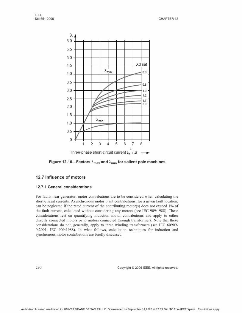
IEEEStd 551-2006 CHAPTER 12
290 Copyright © 2006 IEEE. All rights reserved.
12.7 Influence of motors
12.7.1 General considerations
For faults near generator, motor contributions are to be considered when calculating the
short-circuit currents. Asynchronous motor plant contributions, for a given fault location,
can be neglected if the rated current of the contributing motor(s) does not exceed 1% of
the fault current, calculated without considering any motors (see IEC 909:1988). These
considerations rest on quantifying induction motor contributions and apply to either
directly connected motors or to motors connected through transformers. Note that these
considerations do not, generally, apply to three winding transformers (see IEC 60909-
0:2001, IEC 909:1988). In what follows, calculation techniques for induction and
synchronous motor contributions are briefly discussed.
Figure 12-10—Factors λmax and λmin for salient pole machines
Authorized licensed use limited to: UNIVERSIDADE DE SAO PAULO. Downloaded on September 14,2020 at 17:33:56 UTC from IEEE Xplore. Restrictions apply.

IEEEDEFINITIONS Std 551-2006
Copyright © 2006 IEEE. All rights reserved. 291
12.7.2 Synchronous motors
Synchronous motors and synchronous compensators are to be treated as synchronous
generators, when calculating the initial and peak short-circuit currents. For the case of the
steady-state fault currents, this is applicable only if the synchronous motors’ exciters are
not bus-fed. The same will apply to synchronous compensators. When breaking currents
are calculated, synchronous motor AC decrement is quantitatively modeled as in
generators [see Equation (12.21)]. The ratio r is, however replaced by the ratio m, which
in this case is the ratio of the short-circuit current at the terminals of the motor I"rm to the
rated motor current Irm.
12.7.3 Induction motors
The locked rotor impedance Zm = Rm + jXm of induction motors is given by
Equation (12.25):
(12.25)
where
Urm = Motor rated voltage
Irm = Motor rated current
Ilr = Motor locked rotor current
Srm = Motor rated apparent power
As in the case of synchronous generators, the following X/R ratios are used to account for
both AC and DC decrement of the asynchronous motor contributions:
Xm/Rr = 10.0 with Xm = 0.995Zm (12.26)
For high-voltage motors with power per pair of poles higher or equal to 1 MW.
Xm/Rr = 6.667 with Xm = 0.995 Zm
For high-voltage motors with power per pair of poles less than 1 MW.
Xm/Rr = 2.381 with Xm = 0.922 Zm
For low-voltage motors with connection cables.
When calculating the initial and peak short-circuit currents, asynchronous motors must be
considered. Asynchronous motors are to be ignored when calculating steady-state fault
currents. For breaking current calculations, however, an additional decrement factor is
introduced to account for the rapid flux decay associated with faults at the terminals, as
follows in Equation (12.27):
Xm/Rr = 6.667 with Xm = 0.995 Zm (12.27)
where
Zm1.0 Urm×
Ilr Irm⁄ I× rm 3-------------------------------------
1.0 U× rm2
Ilr Irm⁄ Srm×-------------------------------= =
Authorized licensed use limited to: UNIVERSIDADE DE SAO PAULO. Downloaded on September 14,2020 at 17:33:56 UTC from IEEE Xplore. Restrictions apply.

IEEEStd 551-2006 CHAPTER 12
292 Copyright © 2006 IEEE. All rights reserved.
Ibm = The symmetrical breaking current at time t
I''km = The initial short-circuit current
μ = Decrement factor to time t defined as per Equation (12.22)
q = Decrement factor to time defined as follows:
Xm/Rr = 2.381 with Xm = 0.922 Zm
In Equation (12.27), m is the rated active power in MW of the asynchronous motor per
pair of poles. The maximum value of factor q can attain is 1.00.
The principle of superposition applies to the partial initial, peak and breaking currents
contributed by parallel motors at the common connection point.
12.7.4 Static drives
Static fed regenerative SCR drives are modeled as asynchronous motors with
Zm = According to Equation (12.25)
Urm = Converter transformer rated voltage on network side or
Drive rated voltage in the absence of transformer.
Irm = Converter transformer rated current (network side) or
Drive rated current in the absence of transformer.
I lr / Irm = 3.0 and Xm/Rm = 10.0 with Xm = 0.995 Zm
12.8 Fault calculations in complex systems
In the preceding sections, fault current calculation techniques and methodologies were
outlined for several generic system topologies. When carrying out calculations for a more
complex system, a combination of the above cases is, generally, encountered. For
instance, the short-circuit current may contain not only generator and network feeder
contributions, but also substantial motor (synchronous and asynchronous) content with
varying degrees of electrical proximity to the fault location. The situation may be further
complicated, from a topology point of view, by the fact that several of these sources may
feed the fault through a network portion, comprising many branches, while others may be
directly connected to the short-circuit location. Generally speaking, a combination of the
above stated computational techniques should be used to avoid relaxing several rather
binding clauses of the IEC 909 standard.
12.9 Comparing the ANSI-approved standards with IEC 909
By describing the salient aspects of the IEC 909 standard, one can clearly see that it
departs considerably from its ANSI-approved counterpart, both conceptually and
computational (Rodolakis [B3]). In trying to encapsulate the salient differences, the
following can be concluded:
1) AC decrement modeling is conceptually and computationally different in the two
standards. ANSI favors a universal machine reactance adjustment for calculating
Authorized licensed use limited to: UNIVERSIDADE DE SAO PAULO. Downloaded on September 14,2020 at 17:33:56 UTC from IEEE Xplore. Restrictions apply.

IEEEDEFINITIONS Std 551-2006
Copyright © 2006 IEEE. All rights reserved. 293
the symmetrical interrupting currents. These multipliers are independent of fault
location and breaker parting time. IEC 909:1988 can recommend, instead, taking
into account machine proximity to the short circuit and explicit inclusion of the
parting time.
2) DC decrement modeling is conceptually and computational different in the two
standards. ANSI favors a single approach, based on the X/R ratio at the fault point
featuring separate reactance and resistance reductions of the faulted network. IEC
909 makes a distinction whether independent or not sources feed the fault and rec-
ommends, among other alternative techniques, complex network reductions
whenever a single X/R ratio is to be used.
3) Steady-state fault current calculations are different in the two guidelines due to the
fact that IEC requires explicit consideration of synchronous machinery excitation
systems and saturation influences.
These generic differences in system modeling and computational requirements render the
IEC 909 standard more computationally-intensive that its ANSI-approved counterpart. To
be sure, differences are to be expected, with the IEC 909 standard exhibiting the trend to
be more conservative. If computer simulations are to be performed, the different
computational techniques and data base requirements of the two standards makes it
necessary to use dedicated software.
12.10 Sample calculations
In what follows, the computational and modeling principles outlined in this chapter, are
used to compute three-phase fault currents. The sample system used in Chapter 9, with all
possible sources of short-circuit currents, shall be used for uniformity and ease of
reference. Short circuits on buses 4: MILL-2 (a generator bus), 8: FDRL (a bus with a
synchronous motor) and 37: T14SEC (a bus with induction motors of mixed extraction)
will be simulated. An operating frequency of 60 Hz is assumed. Furthermore, negative
sequence impedances for all rotating plant were assumed to be identical to the positive
sequence impedances.
12.10.1 Rotating equipment impedances
12.10.1.1 Network feeders
There is only one utility service entrance point at 69 kV, situated at bus 100: UTIL-69,
with a fault level of 1000 MVA and an X/R ratio of 22.2. Assuming a 10 MVA power base
for the system, the impedance of the network feeder, per Table 12-1 and Equation (12.1)
is:
or
ZQCVnQ
2
SQ″
-------------1.1 69× 2
1000----------------------= =
Authorized licensed use limited to: UNIVERSIDADE DE SAO PAULO. Downloaded on September 14,2020 at 17:33:56 UTC from IEEE Xplore. Restrictions apply.
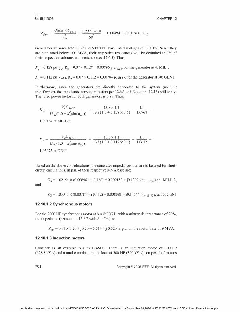
IEEEStd 551-2006 CHAPTER 12
294 Copyright © 2006 IEEE. All rights reserved.
Generators at buses 4:MILL-2 and 50:GEN1 have rated voltages of 13.8 kV. Since they
are both rated below 100 MVA, their respective resistances will be defaulted to 7% of
their respective subtransient reactance (see 12.6.3). Thus,
Xg = 0.128 pu12.5, Rg = 0.07 × 0.128 = 0.00896 p.u.12.5, for the generator at 4: MIL-2
Xg = 0.112 pu15.625, Rg = 0.07 × 0.112 = 0.00784 p..u12.5, for the generator at 50: GEN1
Furthermore, since the generators are directly connected to the system (no unit
transformer), the impedance correction factors per 12.6.3 and Equation (12.16) will apply.
The rated power factor for both generators is 0.85. Thus,
Based on the above considerations, the generator impedances that are to be used for short-
circuit calculations, in p.u. of their respective MVA base are:
ZG = 1.02154 × (0.00896 + j 0.128) = 0.009153 + j0.13076 p.u.12.5, at 4: MILL-2,
and
ZG = 1.03073 × (0.00784 + j 0.112) = 0.008081 + j0.11544 p.u.15.625, at 50: GEN1
12.10.1.2 Synchronous motors
For the 9000 HP synchronous motor at bus 8:FDRL, with a subtransient reactance of 20%,
the impedance (per section 12.6.2 with R = 7%) is:
Zsm = 0.07 × 0.20 + j0.20 = 0.014 + j 0.020 in p.u. on the motor base of 9 MVA.
12.10.1.3 Induction motors
Consider as an example bus 37:T14SEC. There is an induction motor of 700 HP
(678.8 kVA) and a total combined motor load of 300 HP (300 kVA) composed of motors
ZQpuOhms S× Base
VnQ2
---------------------------------5.2371 10×
692
---------------------------- 0.00494 j0.010988 pu10+= = =
KcVcCMAX
UrG 1.0 Xd″ φrG( )sin+( )
--------------------------------------------------------13.8 1.1×
13.8 1.0 0.128 0.6×+( )--------------------------------------------------------
1.1
1.0768----------------
1.02154 at MILL-2
= = = =
KcVcCMAX
UrG 1.0 Xd″ φrG( )sin+( )
--------------------------------------------------------13.8 1.1×
13.8 1.0 0.112 0.6×+( )--------------------------------------------------------
1.1
1.0672----------------
1.03073 at GENI
= = = =
Authorized licensed use limited to: UNIVERSIDADE DE SAO PAULO. Downloaded on September 14,2020 at 17:33:56 UTC from IEEE Xplore. Restrictions apply.

IEEEDEFINITIONS Std 551-2006
Copyright © 2006 IEEE. All rights reserved. 295
rated less than 50 HP. 10 motors, each rated 30 kVA were assumed. All motors run at
1800 rpm, which for a 60 Hz system amounts to two pairs of poles.
For the 700 HP motor the impedance magnitude is calculated as Zm = (0.0139 + j0.167) =
0.1676 p.u. on motor base parameters. Thus, converting to the impedance per the IEC
procedures in section 12.6.3, the motor impedance becomes:
Zm = (0.922 × 0.1676/2.381 + j0.1676 × 0.922) = 0.0649 + j0.1545 p.u.0.6788
Similarly for one 30 HP motor, the impedance magnitude is Zm = (0.0334 + j0.167) =
0.1703 p.u. on motor base parameters. Thus, according to 12.7.3, the motor impedance
becomes:
Zm = (0.922 × 0.1703/2.381 + j0.1703 × 0.922) = 0.0659 + j0.1570 p.u.0.03
The induction motor impedances, for the entire network, were modified per 12.7.3 and the
subclauses that follow depict selected computer-generated results.
12.10.2 Calculation of maximum initial fault currents
12.10.2.1 Fault at bus 4:MILL-2
The equivalent complex impedance at bus 4:MILL-2 is:
ZQQ = 0.00277 = j0.2983 = 0.2996 pu10
The total initial fault current is calculated Equation (12.1) is:
The MILL-2 generator contribution amounts to:
12.10.2.2 Fault at bus 8:FDRL
The equivalent system impedance at bus 8:FDRL was calculated to be ZQQ = 0.033 +
j0.0305 = 0.03068 p.u. on a 10 MVA base. The initial fault current is calculated to be:
with a synchronous motor contribution of
Ik″ CmaxVnpu
ZQQ-----------------------
1.1 1.0×0.02996--------------------- 36.71pu10 I, or 15.36 kA= = = =
IkG″ CmaxVnpu
ZKG-----------------------
1.1 1.0×0.10486--------------------- 10.49pu10 I, or
10.49 10×13.8 3
------------------------- 4.39 kA= = = =
Ik″ CmaxVnpu
ZQQ-----------------------
1.1 1.0×0.03068--------------------- 35.856pu10 I, or
35.856 10×13.8 3
---------------------------- 15.0 kA= = = =
Authorized licensed use limited to: UNIVERSIDADE DE SAO PAULO. Downloaded on September 14,2020 at 17:33:56 UTC from IEEE Xplore. Restrictions apply.
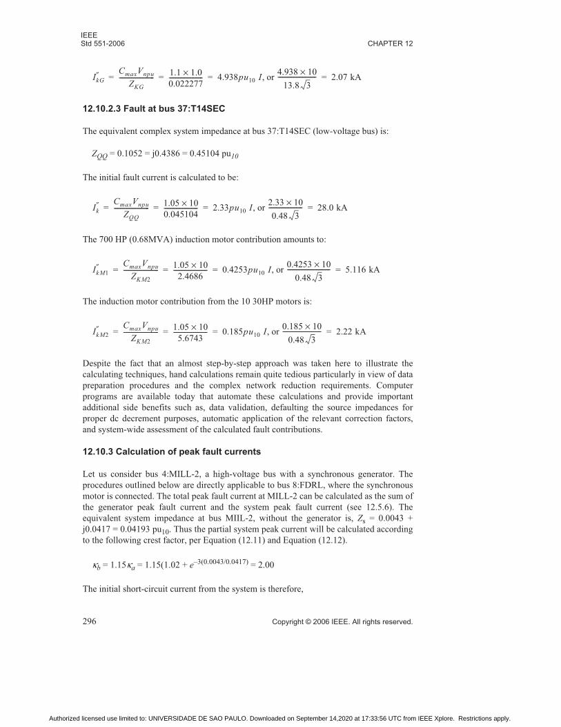
IEEEStd 551-2006 CHAPTER 12
296 Copyright © 2006 IEEE. All rights reserved.
12.10.2.3 Fault at bus 37:T14SEC
The equivalent complex system impedance at bus 37:T14SEC (low-voltage bus) is:
ZQQ = 0.1052 = j0.4386 = 0.45104 pu10
The initial fault current is calculated to be:
The 700 HP (0.68MVA) induction motor contribution amounts to:
The induction motor contribution from the 10 30HP motors is:
Despite the fact that an almost step-by-step approach was taken here to illustrate the
calculating techniques, hand calculations remain quite tedious particularly in view of data
preparation procedures and the complex network reduction requirements. Computer
programs are available today that automate these calculations and provide important
additional side benefits such as, data validation, defaulting the source impedances for
proper dc decrement purposes, automatic application of the relevant correction factors,
and system-wide assessment of the calculated fault contributions.
12.10.3 Calculation of peak fault currents
Let us consider bus 4:MILL-2, a high-voltage bus with a synchronous generator. The
procedures outlined below are directly applicable to bus 8:FDRL, where the synchronous
motor is connected. The total peak fault current at MILL-2 can be calculated as the sum of
the generator peak fault current and the system peak fault current (see 12.5.6). The
equivalent system impedance at bus MIIL-2, without the generator is, Zs = 0.0043 +
j0.0417 = 0.04193 pu10. Thus the partial system peak current will be calculated according
to the following crest factor, per Equation (12.11) and Equation (12.12).
κb = 1.15κa = 1.15(1.02 + e–3(0.0043/0.0417) = 2.00
The initial short-circuit current from the system is therefore,
IkG″ CmaxVnpu
ZKG-----------------------
1.1 1.0×0.022277---------------------- 4.938pu10 I, or
4.938 10×13.8 3
------------------------- 2.07 kA= = = =
Ik″ CmaxVnpu
ZQQ-----------------------
1.05 10×0.045104---------------------- 2.33pu10 I, or
2.33 10×0.48 3
---------------------- 28.0 kA= = = =
IkM1″ CmaxVnpu
ZKM2
-----------------------1.05 10×
2.4686---------------------- 0.4253pu10 I, or
0.4253 10×0.48 3
---------------------------- 5.116 kA= = = =
IkM2″ CmaxVnpu
ZKM2
-----------------------1.05 10×
5.6743---------------------- 0.185pu10 I, or
0.185 10×0.48 3
------------------------- 2.22 kA= = = =
Authorized licensed use limited to: UNIVERSIDADE DE SAO PAULO. Downloaded on September 14,2020 at 17:33:56 UTC from IEEE Xplore. Restrictions apply.

IEEEDEFINITIONS Std 551-2006
Copyright © 2006 IEEE. All rights reserved. 297
Using the above calculated crest factor, per 12.5.3, we obtain
Similarly, the generator crest factor will be:
κGEN = 1.02 + 0.98ε–3 × 0.07 = 1.8143
resulting in a peak current of:
The total peak current at bus 4:MILL-2 is therefore, 31.03 + 11.26 = 42.29 kA.
12.10.4 Calculation of breaking currents
12.10.4.1 Fault at bus 8:FDRL
A three-phase fault is considered at bus 8:FDRL. Assume that the breaking time is 0.02 s
(1.2 cycles). The total breaking current will be composed of the symmetrical rms breaking
current and the unidirectional DC component.
The symmetrical breaking current at bus FDRL is composed of the symmetrical breaking
current of the synchronous motor and of the symmetrical breaking current contributed
from the rest of the system. Assuming no AC decrement for the system contribution, the
breaking current is the initial short-circuit current at bus 8:FDRL with the synchronous
motor disconnected.
The initial fault current is calculated to be:
This current has a DC component of:
Iks″ CmaxVnpu Zqqs 1.1 1.00× 0.04193 26.235pu10, or
26.235 10× 13.8 3( ) 10.97 kA=⁄=⁄=⁄=
Ips κb 2 Iks″
2.00 210.97 31.03 kA== =
IkG″ CmaxVnpu
ZKG-----------------------
1.1 1.0×0.10486--------------------- 10.49pu10 I, or
10.49 10×13.8 3
------------------------- 4.39 kA= = = =
IPGEN κGEN 2 IGEN″
1.8143 2 4.39× 11.26 kA= = =
IbSCmaxVnpu
ZQQ-----------------------
1.1 1.0×0.03559--------------------- 30.9055pu10 I, or
30.9055 10×13.8 3
------------------------------- 12.93 kA= = = =
Idcs 2 Ik″ε 2πftR X⁄–
2 12.93 0.42×× 7.695 kA= = =
Authorized licensed use limited to: UNIVERSIDADE DE SAO PAULO. Downloaded on September 14,2020 at 17:33:56 UTC from IEEE Xplore. Restrictions apply.

IEEEStd 551-2006 CHAPTER 12
298 Copyright © 2006 IEEE. All rights reserved.
The synchronous motor contributes a symmetrical breaking current, which is calculated as
follows (see 12.6.7):
Since r = I"kmr/Irm = 2066/376.53 = 5.487, the decrement factor for a 0.02 s (1.2 cycle)
parting time per Equation (12.12) is as follows:
μ = 0.84 + 0.26ε–0.26r = 0.84 + 0.26ε–0.26 × 5.487 = 0.902
yielding a breaking current of [Equation (12.21)] IbM = μ I"kM = 2.066 × 0.902 =
1.864 kA, with a DC component amounting to the following:
Thus the total symmetrical breaking current at the bus 8:FDRL will be as follows:
Ib = IbS + IbM = 12.9 3kA + 1.724 kA = 14.65 kA
12.10.4.2 Fault at bus 37:T14SEC
The calculation of the total breaking current for bus 37:T14SEC follows the same
procedure as for bus 8:FDRL. For illustration purposes, however, only the symmetrical
breaking currents contributed by the two induction motors will be calculated for a
breaking time of 0.05 s (3 cycles).
For the 700 hp 1800 rpm induction motor using Equation (12.27),
m = HP × 0.746 × MW/HP(1000 × HP × # pole pairs) = 700 × 0.746/2/1000 = 0.261 MW
/pole pair
and factor q = 0.79 + 0.12 Ln(m) = 0.79 + 0.12 Ln(0.261) = 0.6288
Since r = I"km/Irm = 5116/816.47 = 6.26589, the decrement factor for a 0.05 s (3 cycles)
parting time is:
μ = 0.71 + 0.51ε–0.3r = 0.71 + 0.51ε–0.3 × 6.26589 = 0.7878
and the 700 hp motor symmetrical breaking current given by Equation (12.26) is:
Similarly, for the 10 smaller 30 HP, 1800 rpm motors, the following is obtained:
m = HP × 0.746 × MW/HP/(1000 × HP × # pole pairs) = 30 × 0.746/2/1000 =
0.011 MW /pole pair
and factor q = 0.79 + 0.12 Ln(m) = 0.79 + 0.12 Ln(0.011) = 0.2508
Idcs 2 Ik″ε 2πftR X⁄–
2 2.066 0.5899×× 1.724 kA= = =
IbM μqIkM″ 0.7878 0.6288 5.116 2.535 kA=××= =
Authorized licensed use limited to: UNIVERSIDADE DE SAO PAULO. Downloaded on September 14,2020 at 17:33:56 UTC from IEEE Xplore. Restrictions apply.

IEEEDEFINITIONS Std 551-2006
Copyright © 2006 IEEE. All rights reserved. 299
Since r = I"km/Irm = 2225/360.8 = 6.167, the decrement factor for a 0.05 s (3.0 cycle)
parting time is:
μ = 0.71 + 0.51ε–0.3r = 0.71 + 0.51ε–0.3×6.167 = 0.7902
and the 10–30 hp motor symmetrical breaking current given by Equation (12.26) is as
follows:
12.10.5 Calculation of steady-state generator fault currents
Consider the Generator at 4:MILL-2. Assume there is a fault at 4:MILL-2 and that we are
interested in calculating the steady-state fault current contributed by the generator GEN2.
Assuming a saturated reactance of 1.2 p.u. on the generator basis and taking into account
the fact that the generator is of the turbo-alternator type, the following is obtained:
From the Curves of Series 1 (turbo) of the IEC 909:1988 (12.2.1.4) we obtain, λmax = 2.20
for a steady-state fault current from Equation (12.23) of:
Ik max = λmaxIrG = 2.20 × 0.523 = 1.15 kA
From the Curves of Series 2 (turbo) of the IEC 909 (12.2.1.4), we obtain, λmax = 2.70 for
a steady-state fault current of:
Ik max = λmaxIrG = 2.70 × 0.523 = 1.412 kA
12.11 Normative references
The following referenced documents are indispensable for the application of this
document. For dated references, only the edition cited applies. For undated references, the
latest edition of the referenced document (including any amendments or corrigenda)
applies.
IEC 909:1988, Short-Circuit Current Calculation in three-phase a.c. systems. International
Standard (IEC), first edition.2
2IEC publications are available from the Sales Department of the International Electrotechnical Commission,Case Postale 131, 3, rue de Varembé, CH-1211, Genève 20, Switzerland/Suisse (http://www.iec.ch/). IEC publi-cations are also available in the United States from the Sales Department, American National Standards Institute,11 West 42nd Street, 13th Floor, New York, NY 10036, USA.
IbM μqIkM″ 0.7902 0.6288 2.225 0.441=×× kA= =
IrMVA
3kV--------------
12.5
3 13.8×------------------------ 0.523kA
Ir M= VA 3kV( )⁄ 12.5 3 13.8×⁄ 5.523kA= =
r IkG″ IrG⁄ 4389 523 8.392=⁄= =
-------------------------------------------------------------------------------------------------------------------------
rIkG
″
IrG
-------4389
523------------ 8.392= = =
= = =
Authorized licensed use limited to: UNIVERSIDADE DE SAO PAULO. Downloaded on September 14,2020 at 17:33:56 UTC from IEEE Xplore. Restrictions apply.

IEEEStd 551-2006 CHAPTER 12
300 Copyright © 2006 IEEE. All rights reserved.
IEC 60909-0:2001, Short-circuit currents in three-phase systems—Part 0: calculation of
currents.
IEC 61362-1:1998, Guide to specification of hydraulic turbine control systems.
IEC 61363-1:1998, Electrical installations of ships and mobile and fixed offshore units—
Part 1: Procedures for calculating short-circuit currents in three-phase ac.
12.12 Bibliography
[B1] IEC 60038: 1994, IEC standard voltages, Amendment 1.
[B2] IEC 781:1991, Application guide for calculation of short-circuit currents in low-
voltage systems. International Standard (IEC), first edition, 1989.
[B3] Rodolakis, A. J., “A comparison of North American (ANSI) and European (IEC)
Fault Calculation Guidelines,” IEEE Transactions on Industry Applications, Vol. 29, No.
3, pp. 515–521, May/June 1993.
[B4] Roeper, R., Short-Circuit Currents in Three-Phase Systems. Siemens
Actiengesellschaft, John Wiley and Sons, 1985.
Authorized licensed use limited to: UNIVERSIDADE DE SAO PAULO. Downloaded on September 14,2020 at 17:33:56 UTC from IEEE Xplore. Restrictions apply.
Related Documents


