Rebelo Summary

Real Business Cycle Models:Past, Present, and Future∗

Sergio Rebelo†

March 2005

Abstract

In this paper I review the contribution of real business cycles modelsto our understanding of economic fluctuations, and discuss open issues inbusiness cycle research.

∗I thank Martin Eichenbaum, Nir Jaimovich, Bob King, and Per Krusell for their comments,Lyndon Moore and Yuliya Meshcheryakova for research assistance, and the National ScienceFoundation for financial support.

†Northwestern University, NBER, and CEPR.

1. Introduction

Finn Kydland and Edward Prescott introduced not one, but three, revolutionary

ideas in their 1982 paper, “Time to Build and Aggregate Fluctuations.” The first

idea, which builds on prior work by Lucas and Prescott (1971), is that business

cycles can be studied using dynamic general equilibrium models. These models

feature atomistic agents who operate in competitive markets and form rational

expectations about the future. The second idea is that it is possible to unify

business cycle and growth theory by insisting that business cycle models must be

consistent with the empirical regularities of long-run growth. The third idea is

that we can go way beyond the qualitative comparison of model properties with

stylized facts that dominated theoretical work on macroeconomics until 1982.

We can calibrate models with parameters drawn, to the extent possible, from

microeconomic studies and long-run properties of the economy, and we can use

these calibrated models to generate artificial data that we can compare with actual

data.

It is not surprising that a paper with so many new ideas has shaped the

macroeconomics research agenda of the last two decades. The wave of models that

first followed Kydland and Prescott’s (1982) work were referred to as “real business

cycle” models because of their emphasis on the role of real shocks, particularly

technology shocks, in driving business fluctuations. But real business cyle (RBC)

models also became a point of departure for many theories in which technology

shocks do not play a central role.

In addition, RBC-based models came to be widely used as laboratories for

policy analysis in general and for the study of optimal fiscal and monetary pol-

icy in particular.1 These policy applications reflected the fact that RBC models

1See Chari and Kehoe (1999) for a review of the literature on optimal fiscal and monetarypolicy in RBC models.

2

represented an important step in meeting the challenge laid out by Robert Lucas

(Lucas (1980)) when he wrote that “One of the functions of theoretical economics

is to provide fully articulated, artificial economic systems that can serve as labora-

tories in which policies that would be prohibitively expensive to experiment with

in actual economies can be tested out at much lower cost. [...] Our task as I see

it [...] is to write a FORTRAN program that will accept specific economic policy

rules as ‘input’ and will generate as ‘output’ statistics describing the operating

characteristics of time series we care about, which are predicted to result from

these policies.”

In the next section I briefly review the properties of RBC models. It would

have been easy to extend this review into a full-blown survey of the literature. But

I resist this temptation for two reasons. First, King and Rebelo (1999) already

contains a discussion of the RBC literature. Second, and more important, the

best way to celebrate RBC models is not to revel in their past, but to consider

their future. So I devote section III to some of the challenges that face the theory

edifice that has built up on the foundations laid by Kydland and Prescott in 1982.

Section IV concludes.

2. Real Business Cycles

Kydland and Prescott (1982) judge their model by its ability to replicate the

main statistical features of U.S. business cycles. These features are summarized

in Hodrick and Prescott (1980) and are revisited in Kydland and Prescott (1990).

Hodrick and Prescott detrend U.S. macro time series with what became known as

the “HP filter.” They then compute standard deviations, correlations, and serial

correlations of the major macroeconomic aggregates.

Macroeconomists know their main findings by heart. Investment is about three

times more volatile than output, and nondurables consumption is less volatile

3

than output. Total hours worked and output have similar volatility. Almost all

macroeconomic variables are strongly procyclical, i.e. they show a strong con-

temporaneous correlation with output.2 Finally, macroeconomic variables show

substantial persistence. If output is high relative to trend in this quarter, it is

likely to continue above trend in the next quarter.

Kydland and Prescott (1982) find that simulated data from their model show

the same patterns of volatility, persistence, and comovement as are present in

U.S. data. This finding is particularly surprising, because the model abstracts

from monetary policy, which economists such as Friedman (1968) consider an

important element of business fluctuations.

Instead of reproducing the familiar table of standard deviations and correla-

tions based on simulated data, I adopt an alternative strategy to illustrate the

performance of a basic RBC model. This strategy is similar to that used by the

Business Cycle Dating Committee of the National Bureau of Economic Research

(NBER) to compare different recessions (see Hall et al. (2003)) and to the meth-

ods used by Burns and Mitchell (1946) in their pioneer study of the properties of

U.S. business cycles.

I start by simulating the model studied in King, Plosser, and Rebelo (1988) for

5,000 periods, using the calibration in Table 2, column 4 of that paper. This model

is a simplified version of Kydland and Prescott (1982). It eliminates features that

are not central to their main results: time-to-build in investment, non-separable

utility in leisure, and technology shocks that include both a permanent and a

transitory component. I detrend the simulated data with the HP filter. I identify

recessions as periods in which output is below the HP trend for at least three

consecutive quarters.3

2A notable exception is the trade balance which is countercyclical. See Baxter and Crucinni(1993).

3Interestingly, applying this method to U.S. data produces recession dates that are similar to

4

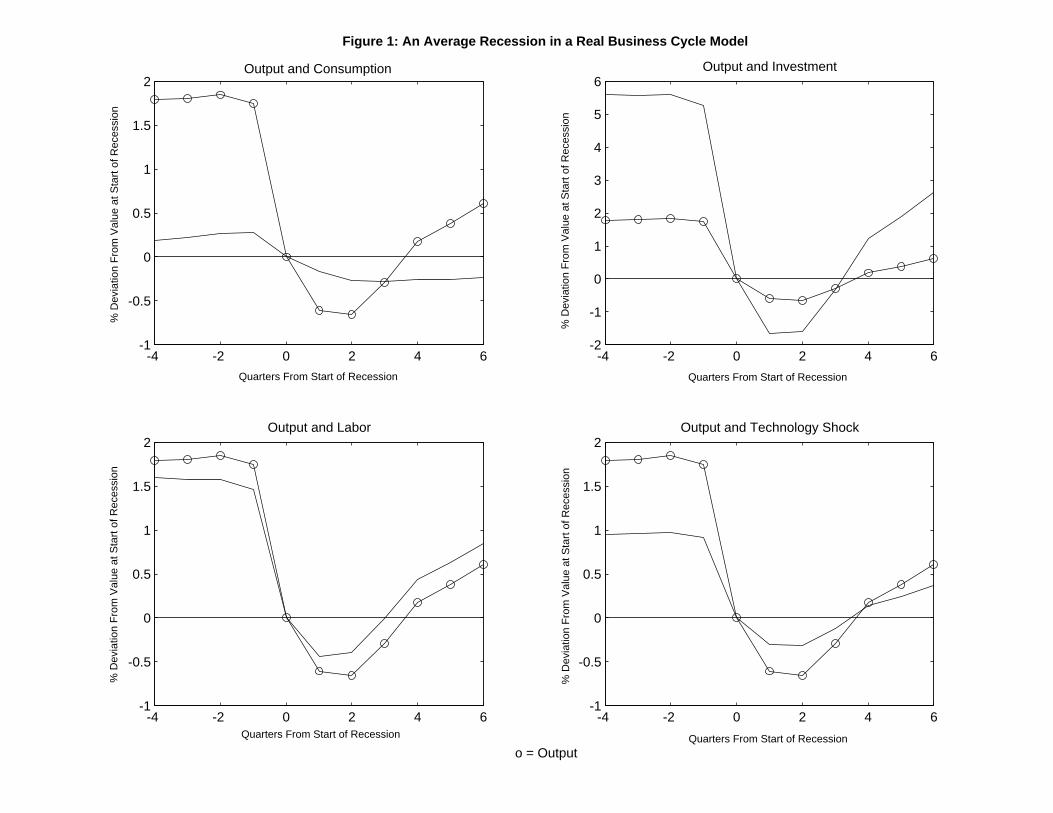
Figure 1 shows the average recession generated by the model. All variables are

represented as deviations from their value in the quarter in which the recession

starts, which I call period zero. This figure shows that the model reproduces the

first-order features of U.S. business cycles. Consumption, investment, and hours

worked are all procyclical. Consumption is less volatile than output, investment

is much more volatile than output, and hours worked are only slightly less volatile

than output. All variables are persistent. One new piece of information I obtain

from Figure 1 is that recessions in the model last for about one year, just as in

the U.S. data.

3. Open Questions in Business Cycle Research

I begin by briefly noting two well-known challenges to RBC models. The first is

explaining the behavior of asset prices. The second is understanding the Great

Depression. I then discuss research on the causes of business cycles, the role of

labor markets, and on explanations for the strong patterns of comovement across

different industries.

The Behavior of Asset Prices Real business cycle models are arguably suc-

cessful at mimicking the cyclical behavior of macroeconomic quantities. However,

Mehra and Prescott (1985) show that utility specifications common in RBC mod-

els have counterfactual implications for asset prices. These utility specifications

are not consistent with the difference between the average return to stocks and

those chosen by the NBER dating committee. The NBER dates for the beginning of a recessionand the dates obtained with the HP procedure (indicated in parentheses) are as follows: 1948-IV (1949-I), 1953-II (1953-IV), 1960-II (1960-III), 1969-IV (1970-I), 1973-III (1974-III), 1981-III(1981-IV), 1990-III (1990-IV), and 2001-I (2001-III). The NBER dates include 1980-I, whichis not selected by the HP procedure. In addition, the HP procedure includes three additionalrecessions starting in 1962-III, 1986-IV, 1995-I. None of the latter episodes involved a fall inoutput.

5

bonds. This “equity premium puzzle” has generated a voluminous literature, re-

cently reviewed by Mehra and Prescott (2003).

Although a generally accepted resolution of the equity premium puzzle is cur-

rently not available, many researchers view the introduction of habit formation

as an important step in addressing some of the first-order dimensions of the puz-

zle. Lucas (1978)-style endowment models, in which preferences feature simple

forms of habit formation, are consistent with the difference in average returns

between stocks and bonds. However, these models generate bond yields that are

too volatile relative to the data.4

Boldrin, Christiano, and Fisher (2001) show that simply introducing habit

formation into a standard RBC model does not resolve the equity premium puz-

zle. Fluctuations in the returns to equity are very small, because the supply of

capital is infinitely elastic. Habit formation introduces a strong desire for smooth

consumption paths, but these smooth paths can be achieved without generating

fluctuations in equity returns. Boldrin, et al. (2001) modify the basic RBC model

to reduce the elasticity of capital supply. In their model investment and con-

sumption goods are produced in different sectors and there are frictions to the

reallocation of capital and labor across sectors. As a result, the desire for smooth

consumption introduced by habit formation generates volatile equity returns and

a large equity premium.

What Caused the Great Depression? The Great Depression was the most

important macroeconomic event of the 20th century. Many economists interpret

the large output decline, stock market crash, and financial crisis that occurred

between 1929 and 1933 as a massive failure of market forces that could have been4Early proponents of habit formation as a solution to the equity premium puzzle include

Sundaresan (1989), Constantinides (1990), and Abel (1990). See Campbell and Cochrane (1999)for a recent discussion of the role of habit formation in consumption-based asset pricing models.

6

prevented had the government played a larger role in the economy. The dramatic

increase in government spending as a fraction of GDP that we have seen since the

1930s is partly a policy response to the Great Depression.

In retrospect, it seems plausible that the Great Depression resulted from an

unusual combination of bad shocks compounded by bad policy. The list of shocks

includes large drops in the world price of agricultural goods, instability in the

financial system, and the worst drought ever recorded. Bad policy was in abundant

supply. The central bank failed to serve as lender of last resort as bank runs forced

many U.S. banks to close. Monetary policy was contractionary in the midst of

the recession. The Smoot-Hawley tariff of 1930, introduced to protect farmers

from declines in world agricultural prices, sparked a bitter tariff war that crippled

international trade. The federal government introduced a massive tax increase

through the Revenue Act of 1932. Competition in both product and labor markets

was undermined by government policies that permitted industry to collude and

increased the bargaining power of unions. Using rudimentary data sources to sort

out the effects of these different shocks and different policies is a daunting task,

but significant progress is being made.5

What Causes Business Cycles? One of the most difficult questions in macro-

economics asks, what are the shocks that cause business fluctuations? Long-

standing suspects are monetary, fiscal, and oil price shocks. To this list Prescott

(1986) adds technology shocks, and argues that they “account for more than half

the fluctuations in the postwar period with a best point estimate near 75%”.

The idea that technology shocks are the central driver of business cycles is con-

troversial. Prescott (1986) computes total factor productivity (TFP) and treats

it as a measure of exogenous technology shocks. However, there are reasons to

5See Christiano, Motto, and Rostagno (2005), Cole and Ohanian (1999, 2004), and theJanuary 2002 issue of the Review of Economic Dynamics and the references therein.

7

distrust TFP as a measure of true shocks to technology. TFP can be forecast us-

ing military spending (Hall (1988)), or monetary policy indicators (Evans (1992)),

both of which are variables that are unlikely to affect the rate of technical progress.

This evidence suggests that TFP, as computed by Prescott, is not a pure exoge-

nous shock, but has some endogenous components. Variable capital utilization,

considered by Basu (1996) and Burnside, Eichenbaum, and Rebelo (1996); vari-

ability in labor effort, considered by Burnside, Eichenbaum, and Rebelo (1993);

and changes in markup rates, considered by Jaimovich (2004a), drive important

wedges between TFP and true technology shocks. These wedges imply that the

magnitude of true technology shocks is likely to be much smaller than that of the

TFP shocks used by Prescott.

Burnside and Eichenbaum (1996), King and Rebelo (1999), and Jaimovich

(2004a) argue that the fact that true technology shocks are smaller than TFP

shocks does not imply that technology shocks are unimportant. Introducing mech-

anisms such as capacity utilization and markup variation in RBC models has two

effects. First, these mechanisms make true technology shocks less volatile than

TFP. Second, they significantly amplify the effects of technology shocks. This

amplification allows models with these mechanisms to generate output volatility

similar to the data with much smaller technology shocks.

Another controversial aspect of RBC models is the role of technology shocks

in generating recessions. The NBER business cycle dating committee defines a

recession as “a significant decline in economic activity spread across the economy,

lasting more than a few months, normally visible in real GDP, real income, em-

ployment, industrial production, and wholesale-retail sales” (Hall et al. (2003)).

Figure 2 shows a histogram of annualized quarterly growth rates of U.S. real GDP.

In absolute terms, output fell in 12 percent of the quarters between 1947 and 2005.

Most RBC models require declines in TFP in order to replicate the declines in

8

output observed in the data.6 Macroeconomists generally agree that expansions

in output, at least in the medium to long run, are driven by TFP increases that

derive from technical progress. In contrast, the notion that recessions are caused

by TFP declines meets with substantial skepticism because, interpreted literally,

it means that recessions are times of technological regress.

Gali (1999) has fueled the debate on the importance of technology shocks as

a business cycle impulse. Gali uses a structural VAR that he identifies by as-

suming that technology shocks are the only source of long-run changes in labor

productivity. He finds that in the short run, hours worked fall in response to a

positive shock to technology. This finding clearly contradicts the implications of

basic RBC models. King, Plosser, and Rebelo (1988) and King (1991) discuss in

detail the property that positive technology shocks raise hours worked in RBC

models. Gali’s results have sparked an animated, ongoing debate. Christiano,

Eichenbaum, and Vigfusson (2003) find that Gali’s results are not robust to spec-

ifying the VAR in terms of the level, as opposed to the first-difference, of hours

worked. Chari, Kehoe, and McGrattan (2004) use a RBC model that fails to

satisfy Gali’s identification assumptions. Their study shows that Gali’s findings

can be the result of misspecification.7 Basu, Fernald, and Kimball (1999) and

Francis and Ramey (2001) complement Gali’s results. They find them robust to

using different data and VAR specifications.

Alternatives to Technology Shocks The debate on the role of technology

shocks in business fluctuations has influenced and inspired research on models in

which technology shocks are either less important or play no role at all. Generally,

6One exception is the model proposed in King and Rebelo (1999), which minimizes the needfor TFP declines in generating recessions. This model requires strong amplification propertiesthat result from a highly elastic supply of labor and utilization of capital.

7See Gali and Rabanal (2005) for a response to the criticisms in Chari, Kehoe, and McGrattan(2004).

9

these lines of research have been strongly influenced by the methods and ideas

developed in the RBC literature. In fact, many of these alternative theories take

the basic RBC model as their point of departure.

Oil Shocks

Movements in oil and energy prices are loosely associated with U.S. recessions

(see Barsky and Killian (2004) for a recent discussion). Kim and Loungani (1992),

Rotemberg and Woodford (1996), and Finn (2000) have studied the effects of

energy price shocks in RBC models. These shocks improve the performance of

RBC models, but they are not a major cause of output fluctuations. Although

energy prices are highly volatile, energy costs are too small as a fraction of value

added for changes in energy prices to have a major impact on economic activity.

Fiscal Shocks

Christiano and Eichenbaum (1992), Baxter and King (1993), Braun (1994),

and McGrattan (1994), among others, have studied the effect of tax rate and

government spending shocks in RBC models. These fiscal shocks improve the

ability of RBC models to replicate both the variability of consumption and hours

worked, and the low correlation between hours worked and average labor pro-

ductivity. Fiscal shocks also increase the volatility of output generated by RBC

models. However, there is not enough cyclical variation in tax rates and govern-

ment spending for fiscal shocks to be a major source of business fluctuations.

While cyclical movements in government spending are small, periods of war are

characterized by large, temporary increases in government spending. Researchers

such as Ohanian (1997) show that RBC models can account for the main macro-

economic features of war episodes: a moderate decline in consumption, a large

decline in investment, and an increase in hours worked. These features emerge

10

naturally in a RBC model in which government spending is financed with lump

sum taxes. Additional government spending has to, sooner or later, be financed

by taxes. Household wealth declines due to the increase in the present value of

household tax liabilities. In response to this decline, households reduce their con-

sumption and increase the number of hours they work, i.e., reduce their leisure.

This increase in hours worked produces a moderate increase in output. Since the

momentary marginal utility of consumption is decreasing, households prefer to

pay for the war-related taxes by reducing consumption both today and in the fu-

ture. Given that the reduction in consumption today plus the expansion in output

are generally smaller than the government spending increase, there is a decline

in investment. Cooley and Ohanian (1997) use a RBC model to compare the

welfare implications of different strategies of war financing. Ramey and Shapiro

(1998) consider the effects of changes in the composition of government spending.

Burnside, Eichenbaum, and Fisher (2004) study the effects of large temporary

increases in government spending in the presence of distortionary taxation.

Investment-specific Technical Change

One natural alternative to technology shocks is investment-specific technolog-

ical change. In standard RBC models, a positive technology shock makes both

labor and existing capital more productive. In contrast, investment-specific tech-

nical progress has no impact on the productivity of old capital goods. Rather, it

makes new capital goods more productive or less expensive, raising the real return

to investment.

We can measure the pace of investment-specific technological change using the

relative price of investment goods in terms of consumption goods. According to

data constructed by Gordon (1990), this relative price has declined dramatically in

the past 40 years. Based on this observation, Greenwood, Hercowitz, and Krusell

11

(1997) use growth accounting methods to argue that 60 percent of postwar growth

in output per man-hour is due to investment-specific technological change. Using

a VAR identified by long-run restrictions, Fisher (2003) finds that investment-

specific technological change accounts for 50 percent of the variation in hours

worked and 40 percent of the variation in output. In contrast, he finds that

technology shocks account for less than 10 percent of the variation in either output

or hours. Starting with Greenwood, Hercowitz, and Krusell (2000) investment-

specific technical change has become a standard shock included in RBC models.

Monetary Models

There are a great many studies that explore the role of monetary shocks in RBC

models that are extended to include additional real elements as well as nominal

frictions.8 Researchers such as Bernanke, Gertler, and Gilchrist (1999) emphasize

the role of credit frictions in influencing the response of the economy to both

technology and monetary shocks. Another important real element is monopolistic

competition, modeled along the lines of Dixit and Stiglitz (1977). In basic RBC

models, firms and workers are price takers in perfectly competitive markets. In

this environment, it is not meaningful to think of firms as choosing prices or

workers as choosing wages. Introducing monopolistic competition in product and

labor markets gives firms and workers nontrivial pricing decisions.

The most important nominal frictions introduced in RBC-based monetary

models are sticky prices and wages. In these models, prices are set by firms

that commit to supplying goods at the posted prices, and wages are set by work-

ers who commit to supplying labor at the posted wages. Prices and wages can

only be changed periodically or at a cost. Firms and workers are forward looking,

8See, for example, Dotsey, King, and Wolman (1999), Altig, Christiano, Eichenbaum, andLinde (2005), and Smets and Wouters (2003). Clarida, Gali, and Gertler (1999) and Christiano,Eichenbaum, and Evans (1999) provide reviews of this literature.

12

so in setting prices and wages, they take into account that it can be too costly, or

simply impossible, to change prices and wages in the near future.

This new generation of RBC-based monetary models can generate impulse

responses to a monetary shock that are similar to the responses estimated using

VAR techniques. In many of these models, technology shocks continue to be

important, but monetary forces play a significant role in shaping the economy’s

response to technology shocks. In fact, both Altig, Christiano, Eichenbaum, and

Linde (2004) and Gali, Lopez-Salido, and Valles (2004) find that in their models, a

large short-run expansionary impact of a technology shock requires that monetary

policy be accommodative.

Multiple Equilibrium Models

Many papers examine models that display multiple rational expectations equi-

libria. Early research on multiple equilibrium relied heavily on overlapping-

generations models, partly because these models can often be studied without

resorting to numerical methods. In contrast, the most recent work on multiple

equilibrium, discussed in Farmer (1999), takes the basic RBC model as a point of

departure and searches for the most plausible modifications that generate multiple

equilibrium.

In basic RBC models, we can compute the competitive equilibrium as a so-

lution to a concave planning problem. This problem has a unique solution, and

so the competitive equilibrium is also unique. When we introduce features such

as externalities, increasing returns to scale, or monopolistic competition, we can

no longer compute the competitive equilibrium by solving a concave planning

problem. Therefore these features open the door to the possibility of multiple

equilibria. Early versions of RBC-based multiple equilibrium models required im-

plausibly high markups or large increasing returns to scale. However, there is

13

a recent vintage of multiple equilibrium models that use more plausible calibra-

tions. (See, for example Wen (1998a), Benhabib and Wen (2003), and Jaimovich

(2004b).)

Multiple equilibrium models have two attractive features. First, since beliefs

are self-fulfilling, belief shocks can generate business cycles. If agents become

pessimistic and think that the economy is going into a recession, the economy

does indeed slowdown. Second, multiple equilibrium models tend to have strong

internal persistence, so such models do not need serially correlated shocks to

generate persistent macroeconomic time series. Starting with a model that has

a unique equilibrium and introducing multiplicity means reducing the absolute

value of characteristic roots from above one to below one. Roots that switch from

outside to inside the unit circle generally assume absolute values close to one, thus

generating large internal persistence.

The strong internal persistence mechanisms of multiple equilibrium models are

a clear advantage vis-à-vis standard RBC models. Although there are exceptions,

such as the model proposed in Wen (1998b), most RBC models have weak internal

persistence. (See Cogley and Nason (1995) for a discussion.) Figure 1 shows that

the dynamics of different variables resemble the dynamics of the technology shock.

Watson (1993) shows that as a result of weak internal persistence, basic RBC

models fail to match the properties of the spectral density of major macroeconomic

aggregates.

An important difficulty with the current generation of multiple equilibrium

models is that they require that beliefs be volatile, but coordinated across agents.

Agents must often change their views about the future, but they must do so in a

coordinated manner. This interest in beliefs has given rise to a literature, surveyed

by Evans and Honkapohja (2001), that studies the process by which agents learn

about the economic environment and form their expectations about the future.

14

Endogenous Business Cycles

The literature on “endogenous business cycles” studies models that generate

business fluctuations, but without relying on exogenous shocks. Fluctuations

result from complicated deterministic dynamics. Boldrin and Woodford (1990)

note that many of these models are based on the neoclassical growth model, and

so have the same basic structure as RBC models. Reichlin (1997) stresses two

difficulties with this line of research. The first is that perfect foresight paths are

extremely complex raising questions as to the plausibility of the perfect foresight

assumption. The second is that models with determinist cycles often exhibit

multiple equilibrium so they are susceptible to the influence of belief shocks.

Other Lines of Research

I finish by describing two promising lines of research that are still in their early

stages. The first line, discussed by Cochrane (1994), explores the possibility that

“news shocks” may be important drivers of business cycles. Suppose that agents

learn that there is a new technology, such as the internet, that will be available in

the future and which is likely to have a significant impact on future productivity.

Does this news generate an expansion today? Suppose that later on, the impact of

this technology is found to be smaller than previously expected. Does this cause

a recession? Beaudry and Portier (2004) show that standard RBC models cannot

generate comovement between consumption and investment in response to news

about future productivity. Future increases in productivity raise the real rate of

return to investing, and, at the same time, generate a positive wealth effect. If

the wealth effect dominates, consumption and leisure rise, and hours worked and

output fall. Since consumption rises and output falls, investment has to fall. If

the real rate of return effect dominates, which happens for a high elasticity of in-

tertemporal substitution, then investment and hours worked rise. However, in this

15

case, output does not increase sufficiently to accommodate the rise in investment

so consumption falls. Beaudry and Portier (2004) take an important first step

in proposing a model that generates the right comovement in response to news

about future increases in productivity. This model requires strong complementar-

ity between durables and nondurables consumption, and abstracts from capital as

an input into the production of investment goods. Producing alternatives to the

Beaudry and Portier model is an interesting challenge to future research.

The second line of research studies the details of the innovation process and its

impact on TFP. Comin and Gertler (2004) extend a RBC model to incorporate

endogenous changes in TFP and in the price of capital that results from research

and development. Although they focus on medium-run cycles, their analysis is

likely to have implications at higher frequencies. More generally, research on the

adoption and diffusion of new technologies is likely to be important in understand-

ing economic expansions.

Labor Markets Most business cycle models require high elasticities of labor

supply to generate fluctuations in aggregate variables of the magnitude that we

observe in the data. In RBC models, these high elasticities are necessary to match

the high variability of hours worked, together with the low variability of real wage

rates or labor productivity. In monetary models, high labor supply elasticities are

required to keep marginal costs flat and reduce the incentives for firms to change

prices in response to a monetary shock. Multiple equilibrium models also rely

on high elasticities of labor supply. If agents believe the economy is entering a

period of expansion, the rate of return on investment must rise to justify the high

level of investment necessary for beliefs to be self-fulfilling. This rise in returns on

investment is more likely to occur if additional workers can be employed without

a substantial increase in real wage rates.

16

Microeconomic studies estimate that the elasticity of labor supply is low.

These estimates have motivated several authors to propose mechanisms that make

a high aggregate elasticity of labor supply compatible with low labor supply elas-

ticities for individual workers. The most widely used mechanism of this kind was

proposed by Rogerson (1988) and implemented by Hansen (1985) in a RBCmodel.

In the Hansen-Rogerson model, labor is indivisible, so workers have to choose be-

tween working full time or not working at all. Rogerson shows that this model

displays a very high aggregate elasticity of labor supply that is independent of the

labor supply elasticity of individual workers. This property results from the fact

that in the model all variation in hours worked comes from the extensive margin,

i.e., from workers moving in and out of the labor force. The elasticity of labor

supply of an individual worker, (i.e. the answer to the question “if your wage

increased by one percent, how many more hours would you choose to work?”) is

irrelevant, because the number of hours worked is not a choice variable.

In RBC-based monetary models, sticky wages are often used to generate a

high elasticity of labor supply. In sticky wage models, nominal wages change only

sporadically and workers commit to supplying labor at the posted wages. In the

short run, firms can employ more hours without paying higher wage rates. But

when firms do so, workers are off their labor supply schedule, working more hours

that they would like, given the wage they are being paid. Consequently, both the

worker and the firm can be better off by renegotiating toward an efficient level of

hours worked. (See Barro (1977) and Hall (2005) for a discussion). More generally,

sticky wage models raise the question of whether wage rates are allocational over

the business cycle. Can firms really employ workers for as many hours as they see

fit at the going nominal wage rate?

Hall (2005) proposes a matching model in which sticky wages can be an equi-

librium outcome. He exploits the fact that in matching models there is a surplus

17

to be shared between the worker and the firm. The conventional assumption in

the literature is that this surplus is divided by a process of Nash bargaining. In-

stead, Hall assumes that the surplus is allocated by keeping the nominal wage

constant. In his model, wages are sticky as long as the nominal wage falls within

the bargaining set. However, there are no opportunities to improve the position

of either the firm or the worker by renegotiating the number of hours worked after

a shock.

Most business cycle models adopt a rudimentary description of the labor mar-

ket. Firms hire workers in competitive spot labor markets and there is no unem-

ployment. The Hansen-Rogerson model does generate unemployment. However,

one unattractive feature of the model is that participation in the labor force is

dictated by a lottery that makes the choice between working and not working

convex.

Two important research topics in the interface between macroeconomics and

labor economics are understanding the role of wages and the dynamics of unem-

ployment. Macroeconomists have made significant process on the latter topic.

Search and matching models, such as the one proposed by Mortensen and Pis-

sarides (1994), have emerged as a framework that is suitable for understanding

not only the dynamics of unemployment, but also the properties of vacancies and

of flows in and out of the labor force. Merz (1995), Andolfatto (1996), Alvarez

and Veracierto (2000), Den Haan, Ramey, and Watson (2000), Gomes, Green-

wood, and Rebelo (2001), and others have incorporated search into RBC models.

However, as discussed by Shimer (2005), there is still work to be done on pro-

ducing a model that can replicate the patterns of comovement and volatility of

unemployment, vacancies, wages, and average labor productivity present in U.S.

data.

18

What Explains Business Cycle Comovement? One of the pioneer papers

in the RBC literature, Long and Plosser (1983), emphasizes the comovement of

different sectors of the economy as an important feature of business cycles. These

authors propose a multisector model that exhibits strong sectoral comovement.

Long and Plosser obtain an elegant analytical solution to their model by assuming

that the momentary utility is logarithmic and the rate of capital depreciation is

100 percent. However, many properties of the model do not generalize once we

move away from the assumption of full depreciation.

Figures 3 and 4 show the strong comovement between employment in different

industries as emphasized by Christiano and Fitzgerald (1998).9 Figure 3 shows

that, with the exception of mining, the correlation between hours worked in the

major sectors of the U.S. economy (construction, durable goods producers, non-

durable goods producers, and services) and aggregate private hours is at least

80 percent. The average correlation is 75 percent. Figure 4 shows that this co-

movement is also present when I consider a more disaggregated classification of

industries. The average correlation of total hours worked in an industry and the

total hours worked in the private sector is 68 percent. The correlation between

industry hours and total hours workers were employed by the private sector is

above roughly 50 except in mining, tobacco, and petroleum and coal. Hornstein

(2000) shows that this sectoral comovement is present in other measures of eco-

nomic activity, such as gross output, value added, and materials and energy use.

These strong patterns of sectoral comovement motivate Lucas (1977) to argue

that business cycles are driven by aggregate shocks, not by sector-specific shocks.

Figures 5 and 6 show that, as discussed in Carlino and Sill (1998) and Koupar-

itsas (2001), there is substantial comovement across regions of the U.S. and across

9I constructed these figures using monthly data from January 1964 to April 2003. I detrendedthe data with the HP filter, using a value of λ of 14, 400. I then used the detrended data tocompute the correlations.

19

different countries.10 The average correlation between Real Gross State prod-

uct and aggregate real GDP for different U.S. states is 58 percent, with only a

small number of states exhibiting low or negative correlation with aggregate out-

put. Figure 6 shows the correlation between detrended GDP the U.S. and the

remaining countries in the G7.11 The average correlation is 46 percent. There is

significant comovement across countries, but this comovement is less impressive

than that across U.S. industries or U.S. states. Backus and Kehoe (1992), Baxter

(1995), and Ambler, Cardia, and Zimmermann (2004) discuss these patterns of

international comovement.

At first sight, it may appear that comovement across different industries is

easy to generate if we are willing to assume there is a productivity shock that is

common to all sectors. However, Christiano and Fitzgerald (1998) show that even

in the presence of a common shock, it is difficult to generate comovement across

industries that produce consumption and investment goods. This difficulty results

from the fact that when there is a technology shock, investment increases by much

more than does consumption. In a standard two-sector model this shock response

implies that labor should move from the consumption sector to the investment sec-

tor. As a result, hours fall in the consumption goods sector in times of expansion.

Greenwood, et al. (2000) show that comovement between investment and con-

sumption industries is also difficult to generate in models with investment-specific

technical change.

One natural way to introduce comovement is to incorporate an input-output

10I computed the correlations reported in Figure 5 using annual data from the Bureau ofEconomic Analysis on Real Gross State Product (GSP) for the period 1977-1997. A discontinuityin the GSP definition prevents me from using the 1998-2003 observations. I detrended the datawith the HP filter, using a λ of 100.11I computed these correlations using annual data for the period 1960-200 from the Heston,

Summers, and Aten (2002) data set for the G7 (data for Germany is for the period 1970-1990).I detrended the data with the HP filter, using a λ of 100.

20

structure into the model (see, for example, Hornstein and Praschnik (1997), Hor-

vath (2000), and Dupor (1999)). However, because input-output matrices are

relatively sparse, intersectoral linkages do not seem to be strong enough to be a

major source of comovement.

Other potential sources of comovement that deserve further exploration are

costs to moving production factors across sectors (Boldrin, et al. (2001)) and

sticky wages (DiCecio (2003)).

The comovement patterns illustrated in Figures 3 through 6 are likely to con-

tain important clues about the shocks and mechanisms that generate business

cycles. Exploring the comovement properties of business cycle models is an im-

portant, but under-researched topic in macroeconomics.

4. Conclusion

Methodological revolutions such as the one led by Kydland and Prescott (1982)

are rare. They propose new methods, ask new questions, and open the door to

exciting research. I was very lucky to have been one of many young researchers

who had a chance to participate in the Kydland-Prescott research program and

get a closer look at the mechanics of business cycles.

21

References

[1] Alvarez, Fernando and Veracierto, Marcelo “Labor Market Policies in an

Equilibrium Search Model,” NBER Macroeconomics Annual 1999, 14: 265-

304, 2000.

[2] Abel, Andrew “Asset Prices under Habit Formation and Catching up with

the Joneses,” American Economic Review, 80: 38—42, 1990.

[3] Altig, David, Lawrence J. Christiano, Martin Eichenbaum, and Jesper Linde

“Firm-Specific Capital, Nominal Rigidities and the Business Cycle,” mimeo,

Northwestern University, 2004.

[4] Ambler, Steve, Emanuela Cardia, and Christian Zimmermann “Interna-

tional Business Cycles: What are the Facts?,” Journal of Monetary Eco-

nomics, 51: 257-276, 2004.

[5] Andolfatto, David “Business Cycles and Labor-Market Search,” American

Economic Review, 86: 112—132, 1996.

[6] Backus, David and Patrick Kehoe “International Evidence on the Historical

Properties of Business Cycles,” American Economic Review, 82: 864-88,

1992.

[7] Barsky, Robert and Lutz Kilian “Oil and the Macroeconomy Since the

1970s,” Journal of Economic Perspectives, 18: 115—134, 2004.

[8] Barro, Robert J. “Long-Term Contracting, Sticky Prices, and Monetary

Policy,”Journal of Monetary Economics, 3: 305—316, 1977.

[9] Basu, Susanto “Procyclical Productivity, Increasing Returns or Cyclical Uti-

lization?,” Quarterly Journal of Economics, 111: 719-751, 1996.

22

[10] Basu, Susanto, John Fernald, and Miles Kimball “Are Technology Improve-

ments Contractionary?,” mimeo, University of Michigan, 1999.

[11] Baxter, Marianne “International Trade and Business Cycles,” in G. Gross-

man and K. Rogoff (eds.) Handbook of International Economics, vol. 3,

1801-64, Elsevier Science Publishers, B.V., Amsterdam, 1995.

[12] Baxter, Marianne, and Mario Crucini “Explaining Saving-investment Cor-

relations,” American Economic Review, 83: 416—436, 1993.

[13] Baxter Marianne, and Robert King “Fiscal Policy in General Equilibrium,”

American Economic Review, 83: 315-334, 1993.

[14] Beaudry, Paul and Franck Portier “An exploration into Pigou’s theory of

cycles,” Journal of Monetary Economics, 51: 1183-1216, 2004.

[15] Benhabib, Jess and Yi Wen “Indeterminacy, Aggregate Demand, and the

Real Business Cycles,” Journal of Monetary Economics, 51: 503-530, 2003.

[16] Bernanke, Ben, Mark Gertler and Simon Gilchrist “The Financial Acceler-

ator in a Quantitative Business Cycle Framework,” Handbook of Macroeco-

nomics, edited by John B. Taylor and Michael Woodford, Amsterdam, New

York and Oxford: Elsevier Science, North-Holland, 1341-93: 1999.

[17] Boldrin, Michelle and Michael Woodford, “Equilibrium Models Displaying

Endogenous Fluctuations and Chaos: A Survey,” Journal of Monetary Eco-

nomics, 25: 189-222, 1990.

[18] Boldrin, Michelle, Lawrence J. Christiano, and Jonas Fisher “Habit Persis-

tence, Asset Returns, and the Business Cycle,” American Economic Review,

91: 149—166, 2001.

23

[19] Braun, R. Anton “Tax Disturbances and Real Economic Activity in the

Postwar United States,” Journal Of Monetary Economics, 33: 441-462,

1994.

[20] Burns, Arthur and Wesley Mitchell Measuring Business Cycles, National

Bureau of Economic Research, New York, 1946.

[21] Burnside, Craig and Martin Eichenbaum “Factor-Hoarding and the Propa-

gation of Business-Cycle Shocks,” American Economic Review, 86: 1154—74,

1996.

[22] Burnside, Craig, Martin Eichenbaum, and Jonas Fisher, “Assessing the Ef-

fects of Fiscal Shocks,” Journal of Economic Theory, 115: 89-117, 2004.

[23] Burnside, Craig, Martin Eichenbaum, and Sergio Rebelo, “Labor Hoarding

and the Business Cycle,” Journal of Political Economy, 101: 245-73, 1993.

[24] Burnside, Craig, Martin Eichenbaum, and Sergio Rebelo “Sectoral Solow

Residuals,” European Economic Review, 40: 861-869, 1996.

[25] Campbell, John and John Cochrane, “By Force of Habit: A Consumption-

based Explanation of Aggregate Stock Market Behavior,” Journal of Polit-

ical Economy, 107: 205—251, 1999.

[26] Carlino, Gerald and Keith Sill “The Cyclical Behavior of Regional Per

Capita Income in the Post War Period,” mimeo, Federal Reserve Bank of

Philadelphia, 1998.

[27] Chari, V. V. and Kehoe, Patrick J., “Optimal Fiscal and Monetary Pol-

icy,” in John B. Taylor and Michael Woodford, eds., Handbook of Macroeco-

nomics, Amsterdam, The Netherlands: Elsevier Science, 1671-1745, 1999.

24

[28] Chari, V. V., Patrick J. Kehoe, and Ellen McGrattan “Are Structural VARs

Useful Guides for Developing Business Cycle Theories?,” Federal Reserve

Bank of Minneapolis,Working Paper 631, 2004.

[29] Christiano, Lawrence and Martin Eichenbaum, “Current Real Business Cy-

cle Theories and Aggregate Labor Market Fluctuations,” American Eco-

nomic Review, 82: 430-50, 1992.

[30] Christiano, Lawrence J. and Terry J. Fitzgerald. “The Business Cycle: It’s

Still a Puzzle,” Federal Reserve Bank of Chicago Economic Perspectives, 22:

56-83, 1998.

[31] Christiano, Lawrence, Martin Eichenbaum, and Robert Vigfusson “What

Happens After a Technology Shock?,” mimeo, Northwestern University,

2003.

[32] Christiano, Lawrence J., Martin Eichenbaum, and Charles Evans “Monetary

Policy Shocks: What Have We Learned and to What End?” in Handbook

of Macroeconomics, vol. 1A, edited by Michael Woodford and John Taylor,

Amsterdam; New York and Oxford: Elsevier Science, North-Holland, 1999.

[33] Christiano, Lawrence, Roberto Motto and Massimo Rostagno, “The Great

Depression and the Friedman-Schwartz Hypothesis,” forthcoming, Journal

of Money, Credit and Banking, 2005.

[34] Clarida, Richard, Jordi Gali, and Mark Gertler, “The Science of Monetary

Policy: A New Keynesian Perspective,” Journal of. Economic Literature,

37: 1661-1707, 1999.

[35] Cochrane, John H. “Shocks,” Carnegie-Rochester Conference Series on Pub-

lic Policy, 41: 295-364, 1994.

25

[36] Cogley, Timothy and James Nason “Output Dynamics in Real Business

Cycle Models,” American Economic Review, 85: 492-511, 1995.

[37] Cole, Harold L. and Lee E. Ohanian “The Great Depression in the United

States From A Neoclassical Perspective,” Federal Reserve Bank of Min-

neapolis Quarterly Review, 23: 2—24, 1999.

[38] Cole, Harold L. and Lee E. Ohanian “New Deal Policies and the Persis-

tence of the Great Depression: A General Equilibrium Analysis,” Journal

of Political Economy, 112: 779-816, 2004.

[39] Cooley, Thomas F., and Lee E. Ohanian. “Postwar British Economic Growth

and the Legacy of Keynes,” Journal of Political Economy, 87: 23-40, 1997.

[40] Comin, Diego and Mark Gertler “Medium Term Business Cycles,” mimeo

New York University, 2004.

[41] Constantinides, George “Habit Formation: A Resolution of the Equity Pre-

mium Puzzle,” Journal of Political Economy, 98: 519—43, 1990.

[42] Den Haan, Wouter, Garey Ramey, and Joel Watson “Job Destruction and

Propagation of Shocks,” American Economic Review, 90: 482—498, 2000.

[43] DiCecio, Riccardo “Comovement: It’s Not a Puzzle,” mimeo, Northwestern

University, November, 2003.

[44] Dixit, Avinash and Joseph Stiglitz “Monopolistic Competition and Opti-

mum Product Diversity,” American Economic Review, 67: 297—308, 1977.

[45] Dotsey, Michael, Robert, G. King, and Alexander L. Wolman, “State-

Dependent Pricing and the General Equilibrium Dynamics of Money and

Output,” Quarterly Journal of Economics, 114: 655-90, 1999.

26

[46] Dupor, Bill, “Aggregation and Irrelevance in Multi-sector Models,” Journal

of Monetary Economics 43: 391—409, 1999.

[47] Evans, Charles L., “Productivity Shocks and Real Business Cycles,” Journal

of Monetary Economics 29: 191-208, 1992.

[48] Evans, George W. and Seppo Honkapohja Learning and Expectations in

Macroeconomics, Princeton University Press, 2001.

[49] Farmer, Roger, Macroeconomics of Self-fulfilling Prophecies, 2nd Edition,

MIT Press, 1999.

[50] Finn, Mary, “Perfect Competition and the Effects of Energy Price Increases

on Economic Activity,” Journal of Money, Credit, and Banking 32: 400-416,

2000.

[51] Fisher, Jonas “Technology Shocks Matter,” mimeo, Federal Reserve Bank

of Chicago, 2003.

[52] Francis, Neville and Valerie Ramey “Is the Technology-Driven Real Business

Cycle Hypothesis Dead? Shocks and Aggregate Fluctuations Revisited, ”

mimeo, University of California, San Diego, 2001.

[53] Friedman, Milton “The Role of Monetary Policy,” The American Economic

Review, 58: 1-17, 1968.

[54] Gali, Jordi “Technology, Employment, and the Business Cycle: Do Technol-

ogy Shocks Explain Aggregate Fluctuations?,” American Economic Review,

89: 249-271, 1999.

27

[55] Gali, Jordi, David Lopez-Salido, and Javier Valles “Technology Shocks and

Monetary Policy: Assessing the Fed’s Performance,” Journal of Monetary

Economics, 50: 723 - 743, 2004.

[56] Gali, Jordi and Pau Rabanal “Technology Shocks and Aggregate Fluctua-

tions: How Well Does the RBC Model Fit Postwar U.S. Data?,” forthcom-

ing, NBER Macroeconomics Annual 2004, 2005 MIT Press.

[57] Gomes, Joao, Jeremy Greenwood, and Sergio Rebelo “Equilibrium Unem-

ployment,” Journal of Monetary Economics, 48: 109—152, 2001.

[58] Gordon, Robert J. The Measurement of Durable Goods Prices, University

of Chicago Press for National Bureau of Economic Research, 1990.

[59] Greenwood, Jeremy, Zvi Hercowitz, and Per Krusell “Long-Run Implications

of Investment-Specific Technological Change,” American Economic Review,

87: 342-362, 1997.

[60] Greenwood, Jeremy, Zvi Hercowitz, and Per Krusell “The Role of

Investment-specific Technological Change in the Business Cycle,” European

Economic Review, 44: 91-115, 2000.

[61] Hall, Robert “The Relation Between Price and Marginal Cost in U.S. In-

dustry,” Journal of Political Economy, 96: 921-47, 1988.

[62] Hall, Robert “Employment Fluctuations with EquilibriumWage Stickiness,”

forthcoming, American Economic Review, 2005.

[63] Hall, Robert, Martin Feldstein, Jeffrey Frankel, Robert Gordon, Christina

Romer, David Romer, and Victor Zarnowitz “The NBER’s Recession Dating

Procedure,” mimeo NBER, 2003.

28

[64] Hansen, Gary D. “Indivisible Labor and the Business Cycle,” Journal of

Monetary Economics, 56: 309—327, 1985.

[65] Heston, Alan, Robert Summers, and Bettina Aten, Penn World Table Ver-

sion 6.1, Center for International Comparisons at the University of Penn-

sylvania, 2002.

[66] Hodrick, Robert and Edward Prescott “Post-war Business Cycles: An Em-

pirical Investigation,” Working Paper, Carnegie-Mellon University, 1980.

[67] Hornstein, Andreas “The Business Cycle and Industry Comovement,” Fed-

eral Reserve Bank of Richmond Economic Quarterly Volume 86/1 Winter

2000.

[68] Hornstein, Andreas and Jack Praschnik “Intermediate Inputs and Sectoral

Comovement in the Business Cycle,” Journal of Monetary Economics, 40:

573—95, 1997.

[69] Horvath, Michael, “Sectoral Shocks and Aggregate Fluctuations,” Journal

of Monetary Economics 45: 69—106, 2000.

[70] Jaimovich, Nir “Firm Dynamics, Markup Variations, and the Business Cy-

cle,” mimeo, University of California, San Diego, 2004a.

[71] Jaimovich, Nir “Firm Dynamics and Markup Variations: Implications for

Multiple Equilibria and Endogenous Economic Fluctuations,” University of

California, San Diego, 2004b.

[72] Kim, In-Moo and Prakash Loungani “The Role of Energy in Real Business

Cycle Models,” Journal of Monetary Economics, 29: 173-90, 1992

29

[73] King, Robert G. “Value and Capital in the Equilibrium Business Cycle

Program,” in Lionel McKenzie and Stefano Zamagni, Value and Capital

Fifty Years Later, MacMillan (London), 1991.

[74] King, Robert, Charles Plosser, and Sergio Rebelo “Production, Growth and

Business Cycles: I. the Basic Neoclassical Model,” Journal of Monetary

Economics, 21: 195-232, 1988.

[75] King, Robert G. and Sergio Rebelo “Resuscitating Real Business Cycles,”

in John Taylor and Michael Woodford, eds., Handbook of Macroeconomics,

volume 1B, 928-1002, 1999.

[76] Kouparitsas, Michael “Is the United States an OptimumCurrency Area? An

Empirical Analysis of Regional Business Cycles,” mimeo, Federal Reserve

Bank of Chicago, 2001.

[77] Kydland, Finn E. and Edward C. Prescott “Time to Build and Aggregate

Fluctuations,“ Econometrica 50: 1345-1370, 1982.

[78] Kydland, Finn E. and Edward C. Prescott “Business Cycles: Real Facts and

a Monetary Myth,” Federal Reserve Bank of Minneapolis Quarterly Review,

14: 3-18, 1990.

[79] Long, John and Charles Plosser “Real Business Cycles,” Journal of Political

Economy, 91: 39-69, 1983.

[80] Lucas, Robert E., Jr. “Asset Prices in an Exchange Economy,” Econometrica

46: 1429—1445, 1978.

[81] Lucas, Robert E., Jr., Understanding Business Cycles, in: K. Brunner and

A. H. Meltzer, eds., Stabilization of the domestic and international economy,

Carnegie-Rochester Conference Series on Public Policy, 5: 7-29, 1977.

30

[82] Lucas, Robert E., Jr. “Methods and Problems in Business Cycle Theory,”

Journal of Money, Credit, and Banking 12: 696-715, 1980.

[83] Lucas, Robert E., Jr., and Prescott, Edward C. “Investment under Uncer-

tainty,” Econometrica, 39: 659-81, 1977.

[84] McGrattan, Ellen R., “The Macroeconomic Effects of Distortionary Taxa-

tion”, Journal of Monetary Economics, 33: 573-601, 1994.

[85] Mehra, Rajnish and Edward C. Prescott “The Equity Premium: A Puzzle,”

Journal of Monetary Economics, 15: 145-161, 1985.

[86] Mehra, Rajnish and Edward C. Prescott “The Equity Premium in Ret-

rospect,” in G. Constantinides, M. Harris and R. Stulz, Handbook of the

Economics of Finance, Elsevier, 2003.

[87] Merz, Monika “Search in the Labor Market and the Real Business Cycle,”

Journal of Monetary Economics, 36: 269—300, 1995.

[88] Mortensen, Dale and Christopher Pissarides, “Job Creation and Job De-

struction in the Theory of Unemployment,”Review of Economic Studies 61,

397-415, 1994.

[89] Ohanian, Lee E. “The Macroeconomic Effects of War Finance in the United

States: World War II and the Korean War,” American Economic Review,

87: 23-40, 1997.

[90] Prescott, Edward “Theory Ahead of Business-Cycle Measurement,”

Carnegie-Rochester Conference Series on Public Policy, 25: 11-44, 1986.

31

[91] Ramey, Valerie A. and Matthew D. Shapiro “Costly Capital Reallocation

and the Effects of Government Spending,” Carnegie-Rochester Conference

Series on Public Policy, 48: 145-194, 1998.

[92] Reichlin, Pietro “Endogenous Cycles in Competitive Models: An Overview,”

Studies in Nonlinear Dynamics and Econometrics, 1:175—185, 1997.

[93] Rogerson, Richard “Indivisible Labor, Lotteries and Equilibrium,” Journal

of Monetary Economics, 21: 3-16, 1988.

[94] Rotemberg, Julio and Michael Woodford “Imperfect Competition and the

Effect of Energy Price Increases on Economic Activity,” Journal of Money

Credit and Banking 28: 549-577, 1996.

[95] Shimer, Robert “The Cyclical Behavior of Equilibrium Unemployment and

Vacancies,” forthcoming, American Economic Review, 2005.

[96] Smets, Frank, and Raf Wouters “An Estimated Dynamic Stochastic General

Equilibrium Model of the Euro Area,” Journal of the European Economic

Association 1: 1123-1175, 2003.

[97] Sundaresan, Suresh M., “Intertemporally Dependent Preferences and the

Volatility of Consumption and Wealth,” Review of Financial Studies 2: 73-

88, 1989.

[98] Watson. Mark “Measures of Fit for Calibrated Models,” Journal of Political

Economy, 101: 1011-1041, 1993.

[99] Wen, Yi, “Capacity Utilization Under Increasing Returns to Scale,” Journal

of Economic Theory, 81: 7-36, 1998a.

32

[100] Wen, Yi “Can a Real Business Cycle Model Pass the Watson Test?,” Journal

of Monetary Economics, 42: 185-203, 1998b.

33

-4 -2 0 2 4 6-1

-0.5

0

0.5

1

1.5

2Output and Consumption

-4 -2 0 2 4 6-2

-1

0

1

2

3

4

5

6Output and Investment

-4 -2 0 2 4 6-1

-0.5

0

0.5

1

1.5

2Output and Labor

-4 -2 0 2 4 6-1

-0.5

0

0.5

1

1.5

2Output and Technology Shock

Quarters From Start of Recession

Figure 1: An Average Recession in a Real Business Cycle Model

o = Output

Quarters From Start of RecessionQuarters From Start of Recession

Quarters From Start of Recession

% D

evia

tion

From

Val

ue a

t Sta

rt of

Rec

essi

on%

Dev

iatio

n Fr

om V

alue

at S

tart

of R

eces

sion

% D

evia

tion

From

Val

ue a

t Sta

rt of

Rec

essi

on%

Dev

iatio

n Fr

om V

alue

at S

tart

of R

eces

sion

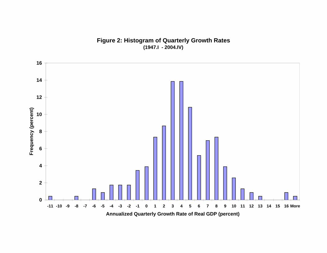
Figure 2: Histogram of Quarterly Growth Rates (1947.I - 2004.IV)

0

2

4

6

8

10

12

14

16

-11 -10 -9 -8 -7 -6 -5 -4 -3 -2 -1 0 1 2 3 4 5 6 7 8 9 10 11 12 13 14 15 16 More

Annualized Quarterly Growth Rate of Real GDP (percent)

Freq

uenc

y (p

erce

nt)

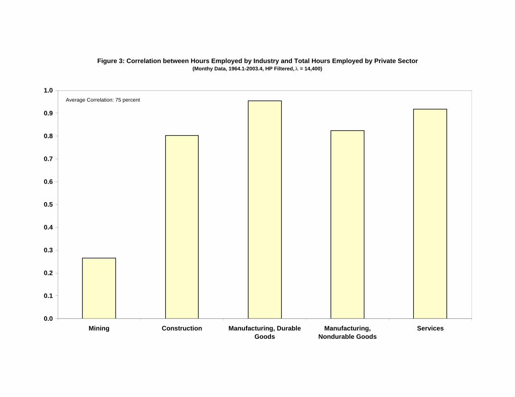
Figure 3: Correlation between Hours Employed by Industry and Total Hours Employed by Private Sector(Monthy Data, 1964.1-2003.4, HP Filtered, λ = 14,400)

0.0

0.1

0.2

0.3

0.4

0.5

0.6

0.7

0.8

0.9

1.0

Mining Construction Manufacturing, DurableGoods

Manufacturing,Nondurable Goods

Services

Average Correlation: 75 percent

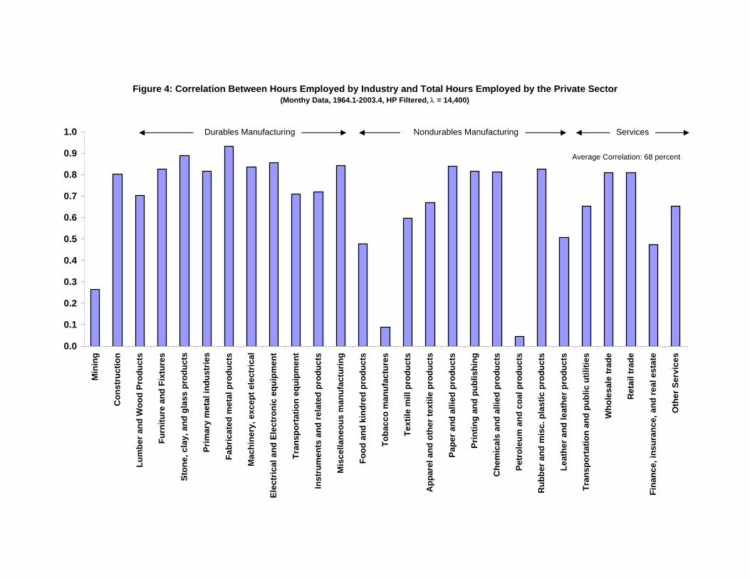
Figure 4: Correlation Between Hours Employed by Industry and Total Hours Employed by the Private Sector(Monthy Data, 1964.1-2003.4, HP Filtered, λ = 14,400)

0.0

0.1

0.2

0.3

0.4

0.5

0.6

0.7

0.8

0.9

1.0

Min

ing

Con

stru

ctio

n

Lum

ber a

nd W

ood

Prod

ucts

Furn

iture

and

Fix

ture

s

Ston

e, c

lay,

and

gla

ss p

rodu

cts

Prim

ary

met

al in

dust

ries

Fabr

icat

ed m

etal

pro

duct

s

Mac

hine

ry, e

xcep

t ele

ctric

al

Elec

tric

al a

nd E

lect

roni

c eq

uipm

ent

Tran

spor

tatio

n eq

uipm

ent

Inst

rum

ents

and

rela

ted

prod

ucts

Mis

cella

neou

s m

anuf

actu

ring

Food

and

kin

dred

pro

duct

s

Toba

cco

man

ufac

ture

s

Text

ile m

ill p

rodu

cts

App

arel

and

oth

er te

xtile

pro

duct

s

Pape

r and

alli

ed p

rodu

cts

Prin

ting

and

publ

ishi

ng

Che

mic

als

and

allie

d pr

oduc

ts

Petr

oleu

m a

nd c

oal p

rodu

cts

Rub

ber a

nd m

isc.

pla

stic

pro

duct

s

Leat

her a

nd le

athe

r pro

duct

s

Tran

spor

tatio

n an

d pu

blic

util

ities

Who

lesa

le tr

ade

Ret

ail t

rade

Fina

nce,

insu

ranc

e, a

nd re

al e

stat

e

Oth

er S

ervi

ces

Average Correlation: 68 percent

Durables Manufacturing Nondurables Manufacturing Services

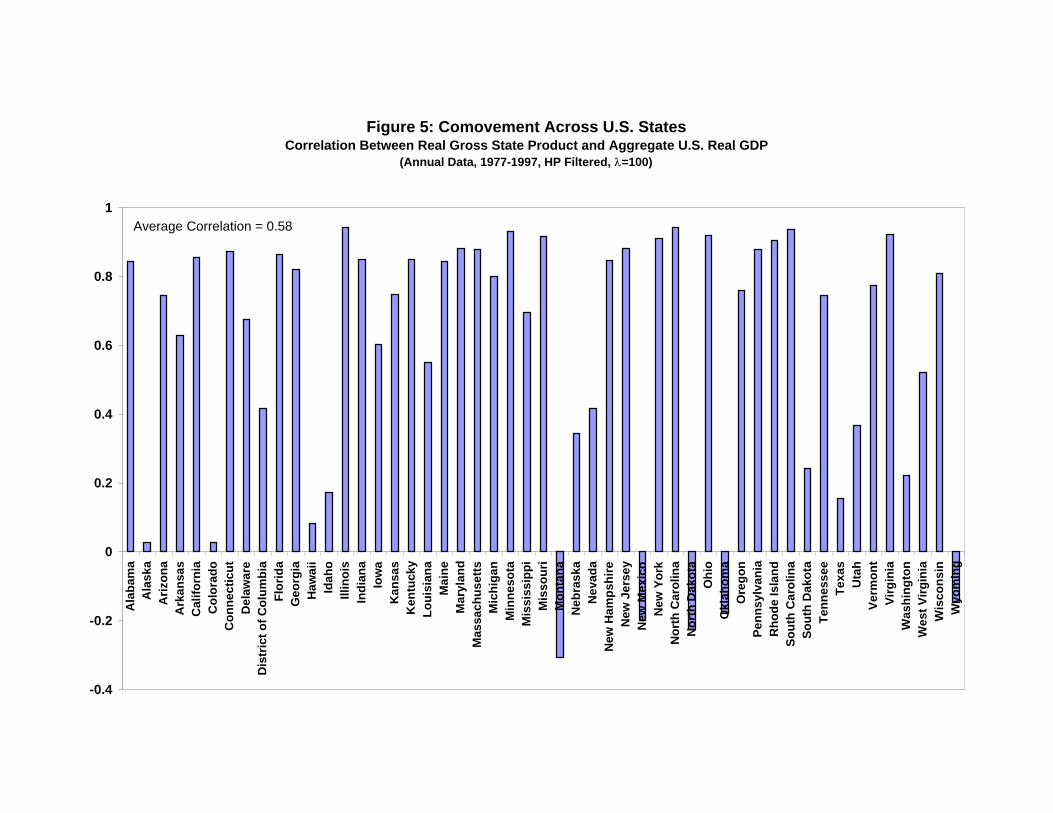
Figure 5: Comovement Across U.S. StatesCorrelation Between Real Gross State Product and Aggregate U.S. Real GDP

(Annual Data, 1977-1997, HP Filtered, λ=100)

-0.4

-0.2

0

0.2

0.4

0.6

0.8

1

Ala

bam

aA

lask

aA

rizon

aA

rkan

sas

Cal

iforn

iaC

olor

ado

Con

nect

icut

Del

awar

eD

istr

ict o

f Col

umbi

aFl

orid

aG

eorg

iaH

awai

iId

aho

Illin

ois

Indi

ana

Iow

aK

ansa

sK

entu

cky

Loui

sian

aM

aine

Mar

ylan

dM

assa

chus

etts

Mic

higa

nM

inne

sota

Mis

siss

ippi

Mis

sour

iM

onta

naN

ebra

ska

Nev

ada

New

Ham

pshi

reN

ew J

erse

yN

ew M

exic

oN

ew Y

ork

Nor

th C

arol

ina

Nor

th D

akot

aO

hio

Okl

ahom

aO

rego

nPe

nnsy

lvan

iaR

hode

Isla

ndSo

uth

Car

olin

aSo

uth

Dak

ota

Tenn

esse

eTe

xas

Uta

hVe

rmon

tVi

rgin

iaW

ashi

ngto

nW

est V

irgin

iaW

isco

nsin

Wyo

min

g

Average Correlation = 0.58

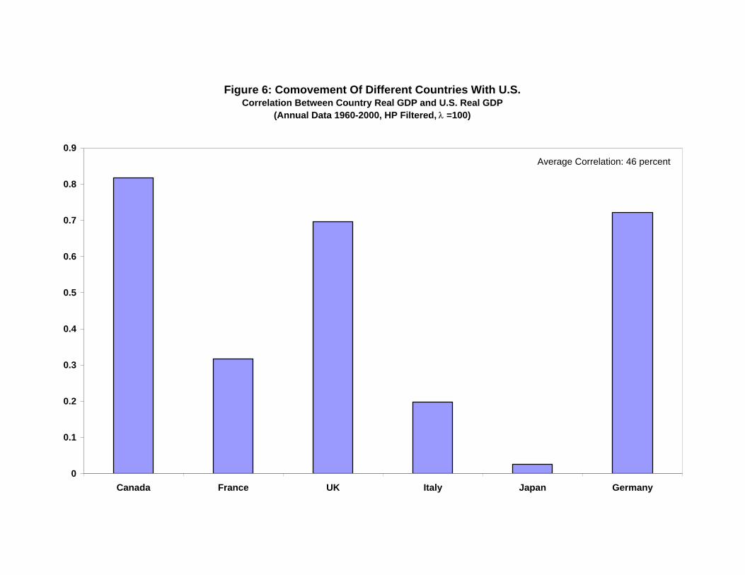
Figure 6: Comovement Of Different Countries With U.S.Correlation Between Country Real GDP and U.S. Real GDP

(Annual Data 1960-2000, HP Filtered, λ =100)

0

0.1

0.2

0.3

0.4

0.5

0.6

0.7

0.8

0.9

Canada France UK Italy Japan Germany

Average Correlation: 46 percent