Reassessing the environmental Kuznets curve for CO2 emissions: A robustness exercise

www.elsevier.com/locate/ecolecon

Ecological Economics 5

ANALYSIS

Reassessing the environmental Kuznets curve for CO2 emissions:

A robustness exerciseB

Marzio Galeotti a,*, Alessandro Lanza b, Francesco Pauli c

a University of Milan and Fondazione Eni Enrico Mattei, Italyb Eni S.p.A. and Fondazione Eni Enrico Mattei, Italy

c University of Trieste and Fondazione Eni Enrico Mattei, Italy

Received 19 May 2004; received in revised form 28 March 2005; accepted 31 March 2005

Available online 15 September 2005

Abstract

The number of studies seeking to empirically characterize the reduced-form relationship between a country economic

growth and the quantity of pollutants produced in the process has recently increased significantly. In several cases, researchers

have found evidence pointing to an inverted-U benvironmental KuznetsQ curve. In the case of CO2, however, the evidence is at

best mixed. In this paper, we reconsider that evidence by assessing how robust it is when the analysis is conducted in a different

parametric setup and when using alternative emissions data, from the International Energy Agency, relative to the literature. Our

contribution can be viewed as a robustness exercise in these two respects. The econometric results lead to two conclusions.

Firstly, published evidence on the EKC does not appear to depend upon the source of the data, at least as far as carbon dioxide is

concerned. Secondly, when an alternative functional form is employed, there is evidence of an inverted-U pattern for the group

of OECD countries, with reasonable turning point, regardless of the data set employed. Not so for non-OECD countries as the

EKC is basically increasing (slowly concave) according to the IEA data and more bellshaped in the case of CDIAC data.

D 2005 Elsevier B.V. All rights reserved.

Keywords: Environment; Growth; CO2 emissions; Panel data

JEL classification: O13; Q30; Q32; C12; C23

0921-8009/$ - see front matter D 2005 Elsevier B.V. All rights reserved.

doi:10.1016/j.ecolecon.2005.03.031

B This paper is part of the research work being carried out by the

Climate Change Modelling and Policy Unit at Fondazione Eni

Enrico Mattei. We acknowledge helpful comments by Andrea Bel-

tratti, Carlo Carrara, Matteo Manera, Michele Pinna, Marcella

Pavan, Lee Schipper, Michael McAleer. This study does not neces-

sarily reflect the views of either Eni S.p.A.

* Corresponding author. Fondazione Eni Enrico Mattei, Corso

Magenta 63, I-20123 Milano, Italy.

E-mail address: [email protected] (M. Galeotti).

1. Introduction

The threat of climate change due to global warm-

ing is an issue whose relevance is by now recognized

by all experts, governments, and public opinions

throughout the world. The 1992 Rio Earth Summit

and the 1997 Kyoto Agreement (along with subse-

quent developments) have called the international

7 (2006) 152–163

M. Galeotti et al. / Ecological Economics 57 (2006) 152–163 153

attention upon the negative consequences as well as

upon the potential instruments to tackle this problem.

One of the most important issues in the policy

arena is related to the role of developing countries.

In fact, while the industrialized countries have agreed

in Kyoto upon an overall 5% reduction in greenhouse

gas emissions relative to 1990 levels, no such com-

mitment has been taken by developing countries.

Whatever the fate of the Kyoto Protocol, underlying

this position, there is a long-standing debate on the

relationship between economic development and

environmental quality. This is quite complicated an

issue to analyze and depends upon a host of different

factors. This fact may explain why most of the work

on the topic, at least until recently, has taken the form

of empirical reduced-form investigations (out of

many, see the survey by Panayotou, 2000).

After the seminal work of Shafik and Bandyopa-

dyay (1992), Selden and Song (1994) and Grossman

and Krueger (1995), several empirical studies have

looked for or identified a bellshaped curve of per

capita pollution relative to per capita GDP. This beha-

vior, known as benvironmental Kuznets curveQ (EKChereafter) implies that, starting from low (per capita)

income levels (per capita) emissions or concentrations

tend to increase but at a slower pace. Beyond a certain

level of income – the bturning pointQ – emissions or

concentrations start to decline as income further

increases.

Although many authors rightly warn about the

non-structural nature of the relationship, if supported

by the data, the inverted-U shape of the curve contains

a powerful message: GDP is both the cause and the

cure of the environmental problem. Among other

things, the argument would provide strong support

for developing countries to resist binding emission

reduction targets such as those envisaged by the

Kyoto Protocol.

Particularly in the case of CO2 emissions, this fact

has such far-reaching implications that extreme cau-

tion and careful scrutiny are necessary when analyz-

ing the issue. Indeed, the global nature of this

pollutant and its crucial role as a major determinant

of the greenhouse effect attribute to the analysis of the

CO2 emissions–income relationship special interest.

Looking at the literature, an initial set of studies

sharing the above characteristics have focused upon

the empirical emergence of a bellshaped EKC and

have typically discussed its implications with special

reference to the level of the income turning point. A

more recent crop of contributions has instead criti-

cized the previous empirical practice and findings, the

most recurrent criticism being the omission of relevant

explanatory variables in the basic relationship.

One aspect that deserves consideration is the issue

of the functional form relating CO2 emissions to GDP.

The norm is second-order or at most-third order poly-

nomial functions for the linear or log-linear models.

However, recently, a few papers have adopted a non-

parametric approach by carrying out kernel regres-

sions (Taskin and Zaim, 2000; Azomahu and Van

Phu, 2001) or a flexible parametric approach (Schma-

lensee et al., 1998; Dijkgraaf and Vollebergh, 2001).

The relative merits of parametric versus non-para-

metric approaches are matter of debate. We do not

pursue this issue here. Instead, we propose and imple-

ment an alternative functional form with appealing

features by way of robustness exercise.

A second contribution of this paper is that we use

data for CO2 emissions that do not come from the

CDIAC. Our data are published by the International

Energy Agency (IEA) of the OECD and are arguably

better than those used by nearly all papers in the

literature. As a matter of fact, we are interested in

assessing the robustness of our empirical results

across the two alternative emissions data series. As

for the rest, we follow the literature and maintain the

typical assumptions that are standard to the EKC

literature. From this point of view, a more fundamen-

tal attack to the very concept of EKC is brought by

Stern in a series of papers (Stern et al., 1996; Stern,

1998, 2004). Besides stressing the econometric con-

sequences of omitted variables for the estimated EKC

parameters, the author notes the lack of rigorous

statistical testing in much of this literature. Although

for some pollutants there seems to be an inverted-U

EKC, he states that the relationship is likely to be a

monotonically increasing one, shifting downward

over time. In a late paper (Perman and Stern, 2003),

on the basis of panel integration and cointegration

tests, this author claims that the EKC does not exist.

In the present paper, as said, we have a simple

goal: we reconsider the evidence in the case of carbon

dioxide emissions by assessing how robust the results

are when the analysis is conducted in a different

parametric setup and using alternative emissions

M. Galeotti et al. / Ecological Economics 57 (2006) 152–163154

data relative to the literature. Our contribution can

therefore be viewed as a robustness exercise in these

two respects.

The structure of this note is the following. Section

2 presents an updated account of the EKC literature

for the case of carbon dioxide. Section 3 discusses the

alternative data on emissions vis-a-vis the standard

data set used by others. In Section 4, we present and

estimate an alternative functional form for the EKC as

well as show the econometric results. Concluding

remarks close the paper.

2. Literature overview

A cursory review of empirical findings in the

specific case of carbon dioxide shows mixed evi-

dence. In early work, Shafik (1994) finds a nearly

monotonic function with a turning point well outside

the sample, while Holtz-Eakin and Selden (1995)

estimate an inverted-U EKC but with an out-of-sam-

ple income turning point of $35,428 in per capita

1986 dollars.1 An EKC model is estimated by Tucker

(1995) for each year of his sample. He finds the

coefficient of the linear income term to be always

positive and significant, while the coefficient of quad-

ratic term is significant in 13 years out of 21, negative

in 11 out of the 13 significant ones, and becomes

negative as time goes by. In this sense, there is an

inverted-U EKC. Sengupta (1996) obtains an N-

shaped relationship and notes that this has implica-

tions for policy, in terms of necessity to set standards/

targets to emissions. Schmalensee et al. (1998) fit a

piecewise linear function (linear spline). There is

evidence of inverted-U shape for the EKC, with the

hypothesis that income parameters of OECD and non-

OECD countries be the same decisively rejected.

Agras and Chapman (1999) include a lagged depen-

dent variable and trade variables, in addition to

income, in their model. Moreover, the fixed effects

are replaced by the energy (gasoline) price. All these

aspects turn out to be statistically important. Galeotti

and Lanza (1999) estimate two alternative parametric

functional forms, Gamma and Weibull, on three sam-

1 Shafik (1994) reports the evidence originally obtained by Shafik

and Bandyopadyay (1992).

ples of data for Annex 1, non-Annex 1 countries, and

the world as a whole. Although they are mostly con-

cerned with emissions forecasts, an inverted-U shape

emerges in all cases.2 Taskin and Zaim (2000) carry

out non-parametric kernel regression on a cross-sec-

tion of data for low-income and high-income coun-

tries. Here a cubic shape is found, i.e., environmental

efficiency initially improves, deteriorates for per

capita income between $5000 and $12,000, and then

improves again. Dijkgraaf and Vollebergh (2001)

challenge the assumption of country homogeneity.

Using data for 24 OECD countries, they decisively

reject the homogeneity hypothesis, even for small

groups of countries. When individual time series mod-

els are estimated, 11 out of 24 cases show a statisti-

cally significant turning point and confirm the

inverted-U EKC pattern. Halkos and Tsionas (2001)

use a switching regime model and Bayesian Markov

chain Monte Carlo methods. In a cross-section of 61

countries, and adding the share of GDP in manufac-

turing, a declining relationship is found between CO2

and GDP. Azomahu and Van Phu (2001) also use a

non-parametric kernel regression method, along with

a standard parametric one, on data for 100 countries.

The authors find that a monotonic relationship cannot

be rejected in the non-parametric model, whereas the

parametric model shows an inverted-U curve. How-

ever, a differencing test rejects the parametric

approach in favor of the non-parametric one. In Hill

and Magnani (2002) (see also Magnani, 2001), the

empirical EKC is shown to be very sensitive to choice

of pollutant, sample of countries, time period. In

particular, for CO2 (156 countries and three separate

years: 1970, 1980, 1990) the results are, (i) from

cross-sections estimation, an inverted-U curve

emerges in all three individual cross-sections, with

the curve moving downward over time periods, (ii)

additional, typically omitted variables, such as educa-

tion, openness and inequality turn out to be all sig-

nificant, (iii) the turning point is very high and near

the upper end of income distribution. Neumayer

(2002) studies the econometric significance of natural

factors such as climatic conditions, availability of

renewable and fossil fuel resources, transportation

2 The Weibull function proposed in Section 3 of this paper is a

generalization of that case.

M. Galeotti et al. / Ecological Economics 57 (2006) 152–163 155

requirements. Using data for 148 countries and a quad-

ratic-log model, the authors find that a bellshaped EKC

exists, but with a turning point well outside range of

GDP values and that natural factors are important,

though income remains the main explanatory variable.

Pauli (2003) notes that unwarranted pooling of coun-

tries may lead to spurious conclusions about EKC. He

therefore uses a new statistical model, a hierarchical

Bayes specification where first level parameters are

country-specific autoregressive. Using data for OECD

countries, he finds that the same model does not fit all

OECD countries; there is a clear monotonic relation-

ship for Greece, Korea, Mexico, Portugal, Turkey, a

decreasing behavior for Luxembourg and Czech

Republic, and a bell shape for France, Germany, UK,

USA, Sweden. Friedl and Getzner (2003) consider the

EKC for a single country, Austria (period 1960–1999),

and come up with a N-shaped relationship with evi-

dence of a structural break in the mid-seventies due to

the oil price shock and additional significant variables

(import share/GDP and services production/GDP

ratios). In addition, emissions and GDP are I(1) and

cointegrated series. Finally, Martinez-Zarzoso and

Bengochea-Morancho (2004) analyze 22 OECD coun-

tries and address the problem of country homogeneity.

The authors use a pooled mean group estimator that

allows for slope heterogeneity in the short run but

imposes restrictions in the long run and test their

validity.3 Their results point to an N-shaped relation-

ship for the majority of countries, but also to a great

heterogeneity among them.

On the basis of the papers just surveyed (and more

generally of the whole EKC literature), we can say

that the typical EKC study has the following features:

(i) besides per capita income, other explanatory vari-

ables are seldom included; (ii) the analysis is usually

conducted on a panel data set of individual countries

around the world; (iii) the data for CO2 emissions

almost invariably come from a single source, the

Carbon Dioxide Information Analysis Center

(CDIAC) of the Oak Ridge National Laboratory;4

(iv) the functional relationship considered is more

often than not either linear or log-linear.

3 This method is also used by Perman and Stern (1999) in the case

of sulfur.4 The data for real per capita GDP are typically drawn from the

Perm World Table and are on a PPP basis.

On the whole, in terms of empirical results, it is fair

to say that the evidence in favor of a reasonable

inverted-U EKC relationship for carbon dioxide is

mixed.

3. Alternative emissions data: a first robustness

check

Our analysis exploits a data set developed by IEA

(International Energy Agency, 2000). It covers the

period between 1960 and 1998 for the Annex II

countries of the United Nations Framework Conven-

tion on Climate Change (Rio de Janeiro, 1992) and

between 1971 and 1998 for all the other countries. In

1997, all countries accounted for nearly 90% of the

CO2 emissions generated by fuel combustion.

As mentioned in the Introduction, the data gener-

ally used in EKC studies concerned with CO2 emis-

sions have been those made available by the Carbon

Dioxide Information Analysis Center (CDIAC) of the

Oak Ridge National Laboratory (Marland et al.,

1998).5 CDIAC distributes and updates a specific

data set concerning global, regional, and national

CO2 emission estimates from fossil fuel burning,

cement production, and gas flaring. The data are

calculated using energy statistics published annually

by the United Nations and using the methods

described in Marland and Rotty (1983). Cement pro-

duction estimates come from the U.S. Department of

Interior’s Bureau of Mines, while gas-flaring esti-

mates are derived principally from United Nations

energy statistics but supplemented with estimates

from the U.S. Department of Energy. The available

data are annual and cover the period 1950–1997.

There are several differences between the CDIAC

data set and the one used in this paper. The IEA data

set is based on energy balances and does not include

either cement production or gas flaring. The impact

of these emissions is however rather small and they

collectively contributed less than 5% to total emis-

sions in 1997. The IEA data set appears to be more

precise mainly because it has used specific emission

coefficients for different energy products, while in

5 Dijkgraaf and Vollebergh (2001) and Pauli (2003) are two othe

examples of use of the IEA data.

r

Table 1

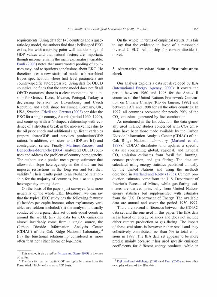
Carbon dioxide emissions–GDP relationship comparison between IEA and CDIAC datasets

OECD Non-OECD Non-OECD Non-OPEC

CDIAC IEA CDIAC IEA CDIAC IEA

GDP �41.93 (�7.27) �62.60 (�6.65) 7.20 (2.10) 6.08 (2.44) 17.62 (3.89) 11.21 (5.16)

GDP square 5.22 (7.93) 7.53 (7.22) �0.74 (�1.76) �0.61 (�2.00) �2.14 (�3.79) �1.33 (�4.90)GDP cube �0.21 (�8.41) �0.30 (�7.71) 0.03 (1.52) 0.02 (1.73) 0.09 (3.78) 0.05 (4.91)

Number of

observations

1070 1064 2256 2317 1959 2020

SSR 40.68 23.00 730.65 192.77 671.93 156.04

Log likelihood �231.04 559.23 �1929.40 �407.03 �1731.61 �279.91Adjusted R2 0.92 0.95 0.87 0.97 0.85 0.97

Turning point 16,487.80 [17.32] 15,697.71 [31.67] – – – –

(1) Dependent variable: log of carbon dioxide emissions per capita; independent variable: log of GDP per capita. Estimated coefficients of

country and time effects not reported.

(2) T-statistics computed from robust standard errors in round brackets. SSR stands for sum of square residuals.

(3) The turning point is expressed in PPP 1990 U.S. dollars. T-ratios in square brackets.

(4) Sample period: 1960–1997 for OECD countries and 1971–1997 for non-OECD countries.

M. Galeotti et al. / Ecological Economics 57 (2006) 152–163156

the CDIAC case, a single coefficient is used for gas,

oil, and solid fossil fuels without any distinction

among individual energy products.6 Quantitatively

speaking, the differences are not significant. The

IEA numbers, however, are slightly bigger than the

CDIAC in both sub-samples. Mean and median values

of CO2 (tons per capita) for CDIAC (IEA) are 8.577

(9.300) and 7.258 (7.662) in the OECD case and

3.538 (4.009) and 1.342 (1.368) in the non-OECD

case respectively.

As for the other variables, the series of Gross

Domestic Product (GDP) and population of the

OECD countries (with the exception of Czech Repub-

6 CO2 emissions associated with a certain fuel are given by the

product of the amount of fuel consumed (so-called bapparent con-sumption,Q AC) times the average carbon content of the fuel (CC)

times the fraction of the fuel which is oxidized in combustion (OF).

This fraction in turn depends upon two factors: inefficiency of

combustion plants (OF1) and non-energy use of the fuel (OF2).

There are several differences in the computation of the above

components between IEA and CDIAC methodologies. As for AC,

the disaggregation of fuel types is higher for CDIAC than for IEA,

but it is not exploited because, on the contrary, the former source

uses fewer CC coefficients: in fact, while IEA uses 27 fuel specific

CC coefficients, CDIAC uses only 3 (liquid, solid, and gas). Note

that these coefficients vary neither over time nor across countries,

with the exception of solid fuels in the IEA approach. Procedures in

the computation of OF1 and OF2 are roughly similar. An appendix

available from the authors provides a more detailed description of

the two methodologies.

lic, Hungary, Poland and the Republic of Korea) come

from the OECD Main Economic Indicators. The cor-

responding series for the other countries have been

obtained from the World Bank.7 GDP is expressed in

1990 U.S. dollars on a PPP basis. Average per capita

GDP was 11,620 U.S. dollars (in 1990 PPP terms) in

OECD countries over the sample period. Non-OECD

regions had instead a value of 4520 USD.8

In order to exploit all available information and,

at the same time, account for the different stage of

economic development, position relative to the tech-

nological frontier, and other structural differences,

we carry out our empirical investigation separately

for the samples of high-income (OECD) and low-

income (non-OECD) countries.9 The distinction

between high-income/OECD and low-income/non-

OECD countries is not totally satisfactory. There are

7 GDP data for the Czech Republic from 1990 onwards come

from the OECD and from 1971 to 1989 are IEA estimates. As said

in a previous footnote, the bulk of the literature uses GDP series

drawn from the Penn World Tables. However, the data publicly

available are limited to 1992. For this reason and in order to focus

more on the differences in emissions data, we use throughout the

same GDP and population data.8 This figure excludes Singapore. If we leave out OPEC countries,

average per capita GDP decreases to 3876 USD.9 There is a number of missing data in our samples either at the

beginning or at the end of the series. In particular, 38 data points are

missing in the OECD sample and 410 in the non-OECD data set

Effective sample sizes are therefore 1093 and 2317 respectively

.

.

M. Galeotti et al. / Ecological Economics 57 (2006) 152–163 157

non-OECD countries with an average per capita

income significantly exceeding that of several

OECD nations. Short of less arbitrary criteria, the

distinction we make here refers not only to income

levels but also to the process and stage of social as

well as economic development. Because high-income

non-OECD countries are primarily oil exporting coun-

tries. It is possible that the statistical results of the

non-OECD group be driven mostly by OPEC regions.

We will therefore present empirical results also for

non-OECD, non-OPEC countries.

The implications of using different emissions data

for the econometric performance of the EKC model

are presented in Table 1. The table shows the results

of estimating a standard cubic log-linear EKC rela-

tionship for a comparable number of countries and

period.10 Looking at the estimated coefficients, we see

that they are rather stable across the two data sets,

both in terms of magnitude and of statistical signifi-

cance. Differences are slightly more pronounced in

the non-OPEC case. A quadratic log-linear model

cannot be rejected for the non-OECD group of coun-

tries, but not so in the more restricted sample. In terms

of goodness of fit, the IEA data seem to produce a

slightly better fit relative to the CDIAC data, espe-

cially in the low-income group. Finally, if we consider

the shape of the estimated EKC curve, we obtain an

inverted-U pattern only for the OECD countries, with

a turning point that is lower when using IEA data.

This point occurs at about fifteen thousand dollars, to

be compared with a mean per capita income in the

sample of about twelve thousand. The non-OECD

sample is instead characterized by an increasing,

slightly concave, relationship.11 On the whole, the

results appear to be similar across the two data sets.

Thus, the conclusion we draw from our first robust-

ness check is that the published evidence on the EKC,

as far as carbon dioxide is concerned, does not appear

to depend upon the generalized use of the same and

single source of CO2 data.

11 While distinguishing between OECD and non-OECD countries

may seem reasonable, Stern and Common (2001) note that signifi-

cant differences in EKC regression results for the two groups of

countries are to be considered as evidence of misspecification.

10 The samples are limited to 1997 because CDIAC data are not

available after that year.

4. An alternative functional form: a second

robustness check

The bulk of the literature assumes that the empiri-

cal relationship between per capita CO2 emissions

and GDP can be adequately described by a para-

metric model, and specifically by a polynomial func-

tion of income. The estimated regression models

have often differed in two respects: (i) the equation

is either linear or log-linear in the variables; (ii) the

equation is either quadratic or cubic. While third-

order polynomial functions allow a high degree of

flexibility, a few recent papers have departed from

the above standard by either using spline functions

or adopting a non-parametric approach altogether.

This is the case, as mentioned, of the papers by

Schmalensee et al. (1998) and Dijkgraaf and Volle-

bergh (2001), who use piecewise linear functions,

and of Taskin and Zaim (2000) and Azomahu and

Van Phu (2001), who carry out kernel regressions. In

particular, a non-parametric approach is in principle

appealing as it imposes no parametric restrictions on

the form of the empirical EKC relationship. While a

sensible strategy, non-parametric approaches have

their own limitations, which include the need of

many data points and the so-called curse of dimen-

sionality which comes into play when more than one

explanatory variable is considered. In this respect,

we do not regard parametric and non-parametric

approaches as perfect substitutes.12

If we confine our attention to the class of para-

metric specifications, we can ask whether there are

alternative functional forms to polynomial functions

that are worth considering. In this section, we propose

one such specification, which is appealing because it

shares the flexibility of third-order polynomials – in

terms of the range of possible shapes which the

relationship under study can possess – and it is char-

acterized by easily interpretable parameters.13 In view

13 A referee has pointed out that easily interpretable parameters are

not an exclusive feature of the functional form proposed here. The

referee offers a clever reparameterization of the quadratic model in

terms three estimable parameters: turning point, curvature, and

maximum level of emissions. Things are more complex, however

in the cubic case.

12 Bradford et al. (2000) is a very recent example of empirical EKC

study using an alternative functional parametric specification.

,

M. Galeotti et al. / Ecological Economics 57 (2006) 152–163158

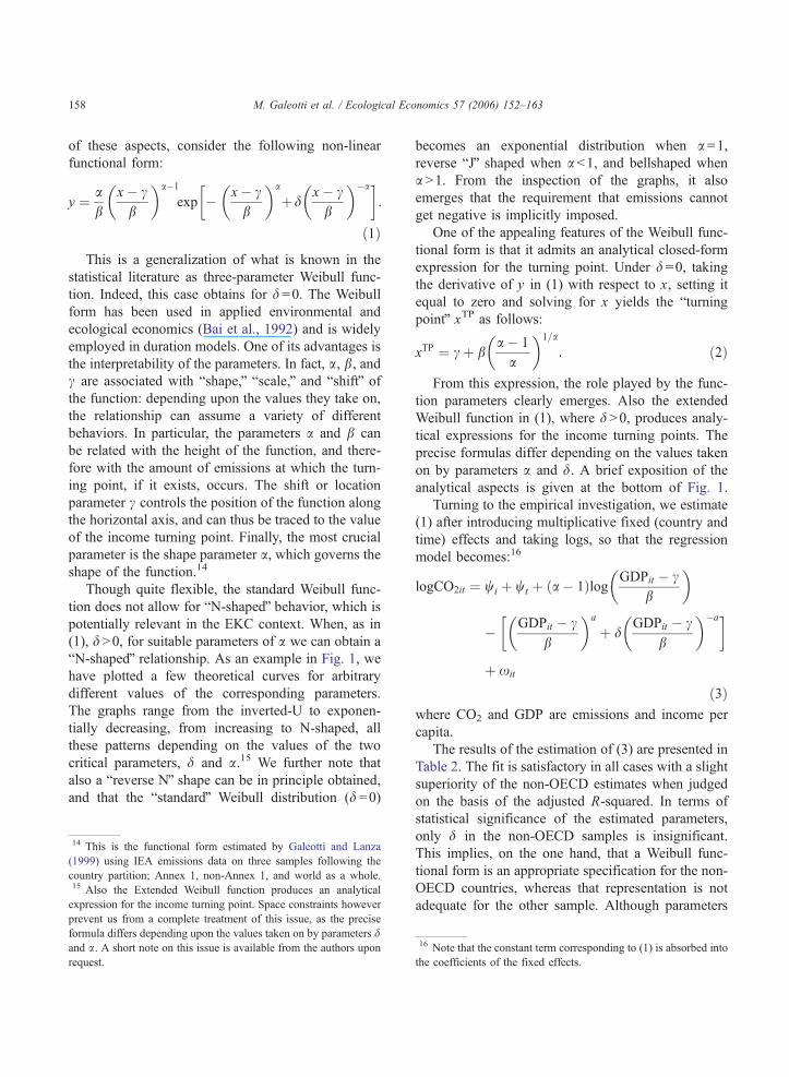
of these aspects, consider the following non-linear

functional form:

y ¼ ab

x� cb

� �a�1exp � x� c

b

� �a

þdx� c

b

� ��a� �:

ð1Þ

This is a generalization of what is known in the

statistical literature as three-parameter Weibull func-

tion. Indeed, this case obtains for d =0. The Weibull

form has been used in applied environmental and

ecological economics (Bai et al., 1992) and is widely

employed in duration models. One of its advantages is

the interpretability of the parameters. In fact, a, b, andc are associated with bshape,Q bscale,Q and bshiftQ ofthe function: depending upon the values they take on,

the relationship can assume a variety of different

behaviors. In particular, the parameters a and b can

be related with the height of the function, and there-

fore with the amount of emissions at which the turn-

ing point, if it exists, occurs. The shift or location

parameter c controls the position of the function along

the horizontal axis, and can thus be traced to the value

of the income turning point. Finally, the most crucial

parameter is the shape parameter a, which governs the

shape of the function.14

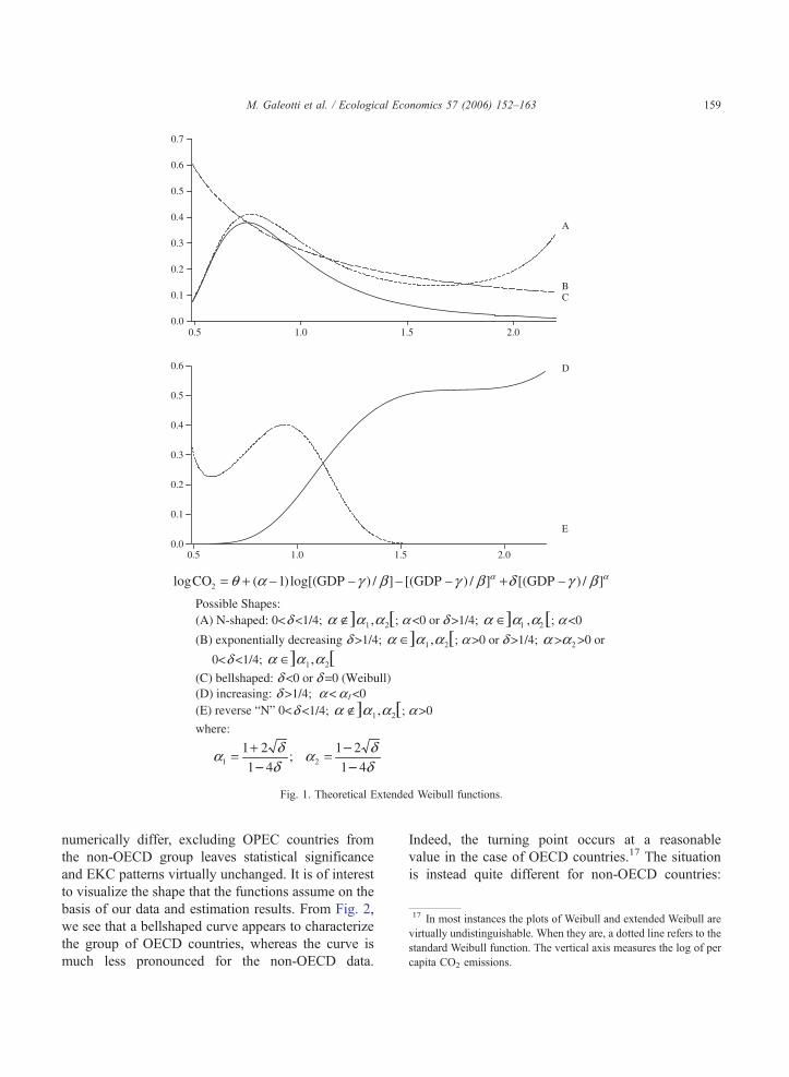
Though quite flexible, the standard Weibull func-

tion does not allow for bN-shapedQ behavior, which is

potentially relevant in the EKC context. When, as in

(1), d N0, for suitable parameters of a we can obtain a

bN-shapedQ relationship. As an example in Fig. 1, we

have plotted a few theoretical curves for arbitrary

different values of the corresponding parameters.

The graphs range from the inverted-U to exponen-

tially decreasing, from increasing to N-shaped, all

these patterns depending on the values of the two

critical parameters, d and a.15 We further note that

also a breverse NQ shape can be in principle obtained,

and that the bstandardQ Weibull distribution (d =0)

15 Also the Extended Weibull function produces an analytical

expression for the income turning point. Space constraints however

prevent us from a complete treatment of this issue, as the precise

formula differs depending upon the values taken on by parameters dand a. A short note on this issue is available from the authors upon

request.

14 This is the functional form estimated by Galeotti and Lanza

(1999) using IEA emissions data on three samples following the

country partition; Annex 1, non-Annex 1, and world as a whole.

becomes an exponential distribution when a =1,reverse bJQ shaped when a b1, and bellshaped when

a N1. From the inspection of the graphs, it also

emerges that the requirement that emissions cannot

get negative is implicitly imposed.

One of the appealing features of the Weibull func-

tional form is that it admits an analytical closed-form

expression for the turning point. Under d =0, takingthe derivative of y in (1) with respect to x, setting it

equal to zero and solving for x yields the bturningpointQ xTP as follows:

xTP ¼ cþ ba� 1

a

� �1=a

: ð2Þ

From this expression, the role played by the func-

tion parameters clearly emerges. Also the extended

Weibull function in (1), where d N0, produces analy-tical expressions for the income turning points. The

precise formulas differ depending on the values taken

on by parameters a and d. A brief exposition of the

analytical aspects is given at the bottom of Fig. 1.

Turning to the empirical investigation, we estimate

(1) after introducing multiplicative fixed (country and

time) effects and taking logs, so that the regression

model becomes:16

logCO2it ¼ wi þ wt þ a� 1ð Þlog GDPit � cb

� �

� GDPit � cb

� �a

þ dGDPit � c

b

� ��a� �

þ xit

ð3Þwhere CO2 and GDP are emissions and income per

capita.

The results of the estimation of (3) are presented in

Table 2. The fit is satisfactory in all cases with a slight

superiority of the non-OECD estimates when judged

on the basis of the adjusted R-squared. In terms of

statistical significance of the estimated parameters,

only d in the non-OECD samples is insignificant.

This implies, on the one hand, that a Weibull func-

tional form is an appropriate specification for the non-

OECD countries, whereas that representation is not

adequate for the other sample. Although parameters

16 Note that the constant term corresponding to (1) is absorbed into

the coefficients of the fixed effects.

αα δαθ [([(log[()1(log 2 +––+=CO

0.0

0.1

0.2

0.3

0.4

0.5

0.6

0.7

0.5 1.0 1.5 2.0

A

B C

0.0

0.1

0.2

0.3

0.4

0.5

0.6

0.5 1.0 1.5 2.0

D

E

Possible Shapes: (A) N-shaped: 0<δ <1/4; ] 21 ,αα ∉ [; α <0 or δ(B) exponentially decreasing

(C) bellshaped: δ <0 or δ =0 (Weibull) (D) increasing: δ >1/4; α < α1 <0 (E) reverse “N” 0<

where:

δδα

δδα

41

21;

41

2121 –

–=–

+=

β ]/)–GDP γ β ]/)–GDP γ β ]/)–GDP γ

α >1/4; ] 21 ,αα ∈ [; α <0αδ >1/4; ]α ∈ [; α >0 or δ >1/4; 2>αα >0 or

0<δ <1/4; ] 21 ,αα ∈ [α

δ <1/4; ] 21 ,αα ∉ α [; α >0

21,αα

Fig. 1. Theoretical Extended Weibull functions.

17 In most instances the plots of Weibull and extended Weibull are

virtually undistinguishable. When they are, a dotted line refers to the

standard Weibull function. The vertical axis measures the log of pe

capita CO2 emissions.

M. Galeotti et al. / Ecological Economics 57 (2006) 152–163 159

numerically differ, excluding OPEC countries from

the non-OECD group leaves statistical significance

and EKC patterns virtually unchanged. It is of interest

to visualize the shape that the functions assume on the

basis of our data and estimation results. From Fig. 2,

we see that a bellshaped curve appears to characterize

the group of OECD countries, whereas the curve is

much less pronounced for the non-OECD data.

Indeed, the turning point occurs at a reasonable

value in the case of OECD countries.17 The situation

is instead quite different for non-OECD countries:

r

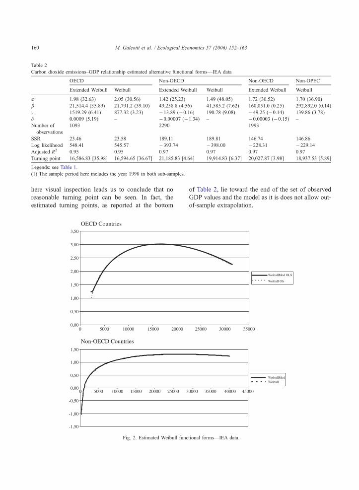
Table 2

Carbon dioxide emissions–GDP relationship estimated alternative functional forms—IEA data

OECD Non-OECD Non-OECD Non-OPEC

Extended Weibull Weibull Extended Weibull Weibull Extended Weibull Weibull

a 1.98 (32.63) 2.05 (30.56) 1.42 (25.23) 1.49 (48.05) 1.72 (30.52) 1.70 (36.90)

b 21,514.4 (35.89) 21,791.2 (39.10) 49,258.8 (4.56) 41,585.2 (7.62) 160,051.0 (0.25) 292,892.0 (0.14)

c 1519.29 (6.41) 877.32 (3.23) �13.89 (�0.16) 190.78 (9.08) �49.25 (�0.14) 139.86 (3.78)

d 0.0009 (5.19) – �0.00007 (�1.34) – �0.00003 (�0.15) –

Number of

observations

1093 2290 1993

SSR 23.46 23.58 189.11 189.81 146.74 146.86

Log likelihood 548.41 545.57 �393.74 �398.00 �228.31 �229.14Adjusted R2 0.95 0.95 0.97 0.97 0.97 0.97

Turning point 16,586.83 [35.98] 16,594.65 [36.67] 21,185.83 [4.64] 19,914.83 [6.37] 20,027.87 [3.98] 18,937.53 [5.89]

Legends: see Table 1.

(1) The sample period here includes the year 1998 in both sub-samples.

M. Galeotti et al. / Ecological Economics 57 (2006) 152–163160

here visual inspection leads us to conclude that no

reasonable turning point can be seen. In fact, the

estimated turning points, as reported at the bottom

OECD Countries

0,00

0,50

1,00

1,50

2,00

2,50

3,00

3,50

0 5000 10000 15000 20000

Non-OECD Countries

-1,50

-1,00

-0,50

0,00

0,50

1,00

1,50

0 5000 10000 15000 20000 25000 3

Fig. 2. Estimated Weibull func

of Table 2, lie toward the end of the set of observed

GDP values and the model as it is does not allow out-

of-sample extrapolation.

25000 30000 35000

WeibullMod OLS

Weibull Ols

0000 35000 40000 45000

WeibullModWeibull

tional forms—IEA data.

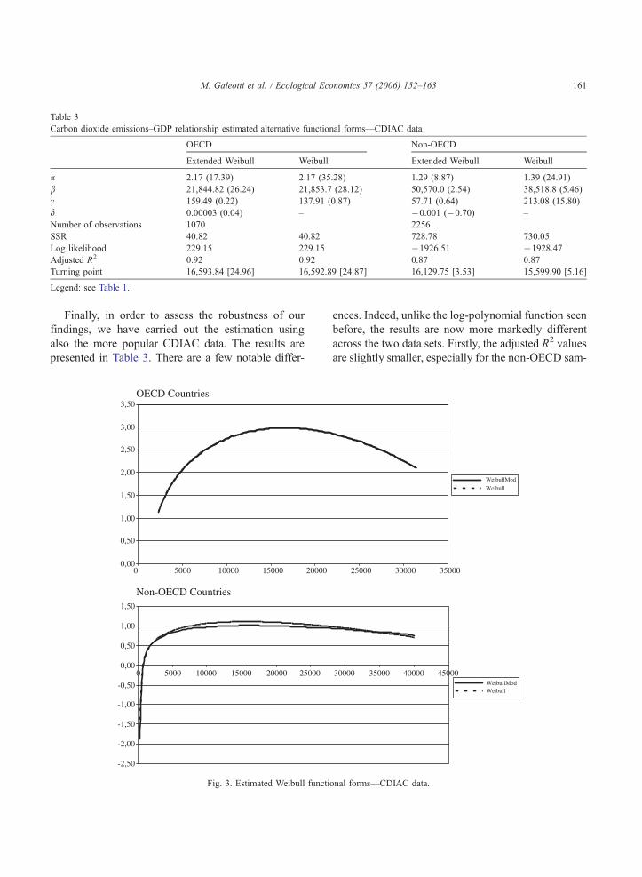
Table 3

Carbon dioxide emissions–GDP relationship estimated alternative functional forms—CDIAC data

OECD Non-OECD

Extended Weibull Weibull Extended Weibull Weibull

a 2.17 (17.39) 2.17 (35.28) 1.29 (8.87) 1.39 (24.91)

b 21,844.82 (26.24) 21,853.7 (28.12) 50,570.0 (2.54) 38,518.8 (5.46)

c 159.49 (0.22) 137.91 (0.87) 57.71 (0.64) 213.08 (15.80)

d 0.00003 (0.04) – �0.001 (�0.70) –

Number of observations 1070 2256

SSR 40.82 40.82 728.78 730.05

Log likelihood 229.15 229.15 �1926.51 �1928.47Adjusted R2 0.92 0.92 0.87 0.87

Turning point 16,593.84 [24.96] 16,592.89 [24.87] 16,129.75 [3.53] 15,599.90 [5.16]

Legend: see Table 1.

M. Galeotti et al. / Ecological Economics 57 (2006) 152–163 161

Finally, in order to assess the robustness of our

findings, we have carried out the estimation using

also the more popular CDIAC data. The results are

presented in Table 3. There are a few notable differ-

OECD Countries

0,00

0,50

1,00

1,50

2,00

2,50

3,00

3,50

0 5000 10000 15000 20000

Non-OECD Countries

-2,50

-2,00

-1,50

-1,00

-0,50

0,00

0,50

1,00

1,50

0 5000 10000 15000 20000 25000

Fig. 3. Estimated Weibull functi

ences. Indeed, unlike the log-polynomial function seen

before, the results are now more markedly different

across the two data sets. Firstly, the adjusted R2 values

are slightly smaller, especially for the non-OECD sam-

25000 30000 35000

WeibullMod

Weibull

30000 35000 40000 45000WeibullModWeibull

onal forms—CDIAC data.

M. Galeotti et al. / Ecological Economics 57 (2006) 152–163162

ple, thus pointing to a somewhat inferior empirical

performance relative to the IEA data. Secondly, the

parameter d is always insignificant, even in the case

of OECD countries, suggesting that a Weibull repre-

sentation is adequate for this data set. Thirdly, and

perhaps more important, the income turning point in

the OECD sample is similar for both IEA and CDIAC

data, while the value corresponding to non-OECD is

much lower and close to that of high-income countries

in the CDIAC sample. As amatter of fact, Fig. 3 reveals

that the EKC for non-OECD countries displays a more

pronounced inverted-U pattern than in the IEA data.

5. Conclusions

The empirical research on the link between emis-

sions of a major greenhouse gas and the degree of

economic development of a country has been recently

spurred by the renewed attention of scientists, policy-

makers, and public opinion to the issue of climate

change. The reduced-form relationship between envir-

onmental degradation and per capita GDP is known as

the environmental Kuznets curve. In the case of CO2

emissions, a few studies have conveniently reported a

bell shape for that relationship. It may be tempting for

somebody to conclude from such evidence, if sup-

ported by the data, that emissions ought to bnaturallyQdiminish as a country becomes richer and richer.

Moreover, identifying the bturning pointQ would

allow the observer to precisely know where his/her

country is located along the curve.

Such inference is unwarranted, though, as it is

based on reduced-form regressions whose results gen-

erally differ across time, space, and even type of

pollutant. In particular, there is econometric evidence

which does not yield an inverted-U EKC, but, rather, a

more problematic N-shaped curve.

In this paper, we have focused on two aspects that,

in the case of carbon dioxide, characterize nearly all

papers in the EKC literature. The first one deserving

consideration is the issue of the functional form relat-

ing CO2 emissions to GDP. The norm is second-order

or at most-third order polynomial functions for the

linear or log-linear models. Here, we have proposed

and implemented an alternative functional form with

appealing features by way of robustness exercise. The

second contribution of this paper is the use of Inter-

national Energy Agency (IEA) data for CO2 emis-

sions, arguably better than the usual CDIAC data.

From these two standpoints, we were interested in

assessing the robustness of the empirical results across

the two alternative emissions data series and across

alternative functional forms. As for the rest, we fol-

lowed the literature and maintained all other typical

assumptions that are standard to the EKC literature.

One critical underlying hypothesis is that, provided

per capita emissions and income are integrated series

of order one, they cointegrate, so that there exists a

stable long run relationship between the two variables.

This is a condition sine qua for the environmental

Kuznets curve to be a meaningful concept (Perman

and Stern, 2003). In this respect, our paper, like many

others, bmaintainsQ rather than btestsQ the integration/

cointegration hypothesis.

Subject to the above caveats, the results presented

here lead to two conclusions. Firstly, published evi-

dence on the EKC does not appear to depend upon the

source of the data, at least as far as carbon dioxide is

concerned, when attention is confined to standard poly-

nomial relationships between per capita emissions and

income. Secondly, when an alternative functional form

is employed, there is evidence of an inverted-U pattern

for the group of OECD countries, with reasonable

turning point, regardless of the data set employed.

Not so for non-OECD countries as the EKC is basically

increasing (slowly concave) according to the IEA data

and more bellshaped in the case of CDIAC data.

On the whole, putting the results of this paper in

the context of the literature and existing available

evidence, the variability of the empirical findings

leads to the conclusion that the underlying statistical

model is rather fragile.

Appendix A. Supplementary data

Supplementary data associated with this article

can be found, in the online version, at doi:10.1016/

j.ecolecon.2005.03.031.

References

Agras, J., Chapman, D., 1999. A dynamic approach to the environ-

mental Kuznets curve hypothesis. Ecological Economics 28,

267–277.

M. Galeotti et al. / Ecological Economics 57 (2006) 152–163 163

Azomahu, T., Van Phu, N., 2001. bEconomic growth and CO2

emissions: a nonparametric approach,Q BETA Working Paper

N.2001-01.

Bai, J., Jakeman, A.J., McAleer, M., 1992. Estimation and discri-

mination of alternative air pollution models. Ecological Model-

ing 64, 89–124.

Bradford, D.F., Schlieckert, R., Shore, S.H., 2000. The environ-

mental Kuznets curve: exploring a fresh specification,QNational Bureau of Economic Research Working Paper

N.8001.

Dijkgraaf, E., Vollebergh, H.R.J., 2001. bA note on testing for

environmental Kuznets curves with panel data,Q Fondazinoe

Eni enrico Mattei Working Paper N. 63.2001.

Friedl, B., Getzner, M., 2003. Determinants of CO2 emissions in a

small open economy. Ecological Economics 45, 133–148.

Galeotti, M., Lanza, A., 1999. Richer and cleaner? A study on

carbon dioxide emissions by developing countries. Energy Pol-

icy 27, 565–573.

Grossman, G., Krueger, A.B., 1995. Economic growth and the

environment. Quarterly Journal of Economics 112, 353–377.

Halkos, G.E., Tsionas, E.G., 2001. Environmental Kuznets curves:

Bayesian evidence from switching regime models. Energy Eco-

nomics 23, 191–201.

Hill, R.J., Magnani, E., 2002. An exploration of the conceptual and

empirical basis of the environmental Kuznets curve. Australian

Economic Papers 41, 239–254.

Holtz-Eakin, D., Selden, T.M., 1995. Stoking the fires? CO2 emis-

sions and economic growth. Journal of Public Economics 57,

85–101.

International Energy Agency, 2000. CO2 Emissions from Fuel

Combustion, A New Basis for Comparing Emissions of a

Major Greenhouse Gas. International Energy Agency, Paris.

Magnani, E., 2001. The environmental Kuznets curve: development

path or policy result? Environmental Modeling and Software 16,

157–165.

Marland, G., Rotty, R.M., 1983. bCarbon dioxide emissions from

fossil fuels: a procedure for estimation and results for 1950–

1981,Q DOE/NBB-0036, TR003, U. S. Department of Energy,

Washington, D.C.

Marland, G., Andres, R.J., Boden, T.A., Johnston, C., Brenkert, A.,

1998. bGlobal, regional, and national CO2 emission estimates

from fossil fuel burning, cement production, and gas flaring:

1751–1995,Q Carbon Dioxide Information Analysis Center, Oak

Ridge National Laboratory, Oak Ridge, Tennessee, Report No.

ORNL/CDICA-30.

Martinez-Zarzoso, I., Bengochea-Morancho, A., 2004. Pooled mean

group estimation for an environmental Kuznets curve for CO2.

Economics Letters 82, 121–126.

Neumayer, E., 2002. Can natural factors explain any cross-coun-

try differences in carbon dioxide emissions? Energy Policy

30, 7–12.

Panayotou, T., 2000. bEconomic growth and the environment,QCenter for International Development, Harvard University,

Environment and Development Paper N.4.

Pauli, F., 2003. bEnvironmental Kuznet investigation using a vary-

ing coefficient AR model,Q Abdus Salam International Centre

for Theoretical Physics EEE Working Paper No. 12.

Perman, R., Stern, D.I., 1999. The environmental Kuznets curve:

implications of non-stationarity, Centre for Resource and Envir-

onmental Studies, Working Papers in Ecological Economics

No. 9901.

Perman, R., Stern, D.I., 2003. Evidence from panel unit root and

cointegration tests that the environmental Kuznets curve does

not exist. Australian Journal of Agricultural and Resource Eco-

nomics 47, 325–347.

Schmalensee, R., Stoker, T.M., Judson, R.A., 1998. World carbon

dioxide emissions: 1950–2050. Review of Economics and Sta-

tistics LXXX, 15–27.

Selden, T.M., Song, D., 1994. Environmental quality and develop-

ment: is there a Kuznets curve for air pollution emissions.

Journal of Environmental Economics and Management 27,

147–162.

Sengupta, R., 1996. CO2 emission–income relationship: policy

approach for climate control. Pacific and Asian Journal of

Energy 7, 207–229.

Shafik, N., 1994. Economic development and environmental qual-

ity: an econometric analysis. Oxford Economic Papers 46,

757–773.

Shafik, N., Bandyopadyay, S., 1992. bEconomic growth and envir-

onmental quality,Q Background Paper for the 1992 World Devel-

opment Report, The World Bank, Washington, D.C.

Stern, D.I., 1998. Progress on the environmental Kuznets curve?

Environment and Development Economics 3, 173–196.

Stern, D.I., 2004. The rise and fall of the environmental Kuznets

curve. World Development 32, 1419–1439.

Stern, D.I., Common, M.S., 2001. Is there an environmental Kuz-

nets curve for sulphur? Journal of Environmental Economics

and Management 14, 162–178.

Stern, D.I., Common, M.S., Barbier, E.B., 1996. Economic growth

and environmental degradation: the environmental Kuznets

curve and sustainable development. World Development 24,

1151–1160.

Taskin, F., Zaim, O., 2000. Searching for a Kuznets curve in

environmental efficiency using Kernel estimation. Economics

Letters 68, 217–223.

Tucker, M., 1995. Carbon dioxide emissions and global GDP.

Ecological Economics 15, 215–223.