Really Uncertain Business Cycles

Really Uncertain Business Cycles

Nicholas Bloom, Max Floetotto and Nir Jaimovich�

Stanford University

July 2009

Abstract

We propose uncertainty shocks as an additional impulse driving business cycles.First, we demonstrate that uncertainty, measured by a number of proxies, appears tobe strongly countercyclical. When uncertainty is included in a standard vector au-toregression, increases in uncertainty lead to a large drop and subsequent rebound ineconomic activity. Second, we build a dynamic stochastic general equilibrium modelthat extends the benchmark neoclassical growth model along two dimensions. It allowsfor the existence of heterogeneous �rms with non-convex adjustment costs in both capi-tal and labor, as well as time-variation in uncertainty that is modeled as a change in thevariance of innovations to productivity. We �nd that increases in uncertainty lead tolarge drops in economic activity. This occurs because a rise in uncertainty makes �rmscautious, leading them to pause hiring and investment, and reduces the reallocation ofcapital and labor across �rms, leading to a large fall in productivity growth. Finally, weshow that uncertainty signi�cantly reduces the response of the economy to stimulativepolicy, relative to its response during low uncertainty periods. This implies that in orderfor policy during high uncertainty periods to have the same e¤ect it would as under lowuncertainty periods, the policy impulse should be signi�cantly larger and temporary.

Keywords: uncertainty, adjustment costs and business cycles.JEL Classi�cation: D92, E22, D8, C23.

�We would like to thank our formal discussant Eduardo Engel and participants at the AEA for commentsand suggestions. Correspondence: Nick Bloom, Department of Economics, Stanford University, Stanford,CA 94305, [email protected].

1 Introduction

In this paper we study the implications of variations in the level of uncertainty, or second-

moment shocks, for business cycles. The idea to link uncertainty to the business cycle is

not new. John Maynard Keynes (1936) argued that changes in investor sentiments, the

so-called animal spirits, could lead to economic downturns. While this can be interpreted

as an argument for the role of uncertainty, it has not traditionally played a large role in

modern studies of business cycle �uctuations.

This paper attempts to �ll this gap by taking two distinct steps. First, we address

the empirical behavior of uncertainty over the business cycle. Evidence on the time series

variation in uncertainty is scarce, as no measure of uncertainty is directly observable. To

circumvent this di¢ culty, we use various proxies for uncertainty that include measures of

cross-�rm and cross-industry dispersion, time series variation of aggregate data, as well as

measures of forecaster disagreement. We �nd that all of our uncertainty proxies are strongly

countercyclical, and when combined into a single uncertainty index, we �nd that this index

increases by 48% during recessions.1 We then investigate the conditional association of

uncertainty and the business cycle by including the uncertainty index in a standard vector

autoregression (VAR), and �nd that an increase in uncertainty is associated with a large

drop and subsequent rebound in economic activity.

Since it is hard to argue that our uncertainty index is completely exogenous, we use

the second part of the paper to theoretically investigate the role of �uctuations in uncer-

tainty since we can, by assumption within our model, assure the exogeneity of uncertainty

shocks. Speci�cally, we study a dynamic stochastic general equilibrium model that allows

for shocks to both the level of technology (the �rst moment) as well as uncertainty (the

second moment), where the latter are modeled as variation in the standard deviation of the

innovations to productivity. Various features of the model are speci�ed to conform as closely

as possible to the standard frictionless neoclassical growth model. The main deviation from

this frictionless benchmark model lies in assuming that heterogeneous �rms incur convex

and non-convex adjustment costs in both capital and labor. The non-convexities imply that

�rms become more cautious in investing and hiring when uncertainty increases due to the

option value of waiting, which increases when uncertainty is high since it is expensive for

�rms to invest and then disinvest or to hire and then �re. The time-varying option value im-

plies that, in the presence of higher aggregate macro uncertainty, aggregate investment and

employment levels fall as it becomes optimal for each individual �rm to wait. In addition,

we show that time-varying uncertainty reduces productivity growth during times of high

uncertainty because it lowers the extent of reallocation in the economy; when uncertainty

1This index is constructed as a simple average of our seven proxies after re-scaling each of them to an averageof one in non-recession periods.

1

rises, productive �rms expand less and unproductive �rms contract less.2 It is important

to emphasize that we do not claim that other mechanisms that cause �uctuations in uncer-

tainty and that can a¤ect economic activity are irrelevant. Rather, we emphasize a speci�c

mechanism in a model that encompasses the standard perfect competition, real business

cycle (RBC) model, as this greatly simpli�es comparison with existing work.

We then build on our theoretical model to investigate the e¤ects of uncertainty on

policy e¤ectiveness. We use a simple illustrative example to show the presence signi�cantly

dampens the e¤ect of an expansionary policy.

Our work is related to several strands in the literature. First, we add to the extensive

literature building on the RBC framework by studying the role of productivity (TFP) shocks

in causing business cycles. In the standard RBC literature, recessions are caused by large

negative technology shocks.3 The reliance on negative technology shocks has proven to be

controversial, as it suggests that recessions are times of technological regress. To quote

King and Rebelo (1999): �If these shocks are large and important, why can�t we read about

them in the Wall Street Journal?�4 As discussed above, our work provides a rationale for

falls in measured productivity. Countercyclical increases in uncertainty lead to a freeze

in economic activity, substantially lowering productivity growth during recessions. In our

model, however, the drop in productivity is not causing the recession, but rather it is an

artifact of a recession that was caused by an increase in uncertainty.

The paper also relates to the literature on investment under uncertainty. A growing

body of work has shown that uncertainty can directly in�uence �rm-level investment and

employment in the presence of adjustment costs.5 The most relevant paper is Bloom (2009),

which solves a partial equilibrium model with stochastic volatility and shows how uncer-

tainty shocks lead to a drop in investment and hiring by �rms. Our paper is di¤erent in

that we are looking at the business cycle in a general equilibrium framework.

Finally, the paper is related to the literature studying macroeconomic models with

micro-rigidities.6 The paper contributes to this literature by �nding that in the presence

2 In the actual U.S. economy, reallocation is a key factor driving aggregate productivity. See, for example,Foster, Haltiwanger and Krizan (2000, 2006), who report that reallocation, broadly de�ned to include entryand exit, accounts for around 50% of manufacturing and 80% of retail productivity growth in the US.3See, for example, the discussion in Rebelo (2005): �Most RBC models require declines in TFP in order toreplicate the declines in output observed in the data.�4This reasoning has lead many researchers to study models with other disturbances, which mostly focus on�rst-moment (level) shocks. A partial list of these alternative shocks includes oil shocks, investment speci�cshocks, monetary shocks, government expenditure shocks, news shocks, and terms-of-trade shocks. Yet, inmost models, negative technology shocks continue to be an important driver of economic downturns.5See, for example; Bernanke (1983), Pindyck (1988), Dixit (1990), Bertola and Bentolila (1990), Bertola andCaballero (1994), Dixit and Pindyck (1994), Abel and Eberly (1996), Hassler (1996), and Caballero andEngel (1999).6See for example, Thomas (2002), Veraciertio (2002), Kahn and Thomas (2006 and 2008), Bachman, Caballeroand Engel (2008), and House (2008).

2

of time-varying uncertainty, micro-rigidities of the type considered here (i.e., non-convex

adjustment costs) have important general equilibrium e¤ects.

The remainder of this paper is organized as follows. Section 2 discusses the behavior

of uncertainty over the business cycle. In Section 3 we formally present the model and de-

�ne the recursive equilibrium. Since most of the business cycle literature has concentrated

exclusively on �rst-moment shocks where the level of uncertainty is held constant, we de-

part from the standard log-linearization techniques and use non-linear methods instead.

Speci�cally, section 3.4 presents our solution algorithm which builds on the work of Krusell

and Smith (1998), Kahn and Thomas (2008) and Bachman, Caballero and Engel (2008).

The model is calibrated and simulated in Section 4, where we study the role of uncertainty

shocks in driving the business cycle. Section 5 studies the impact of policy shocks in the

presence of time-varying uncertainty. Section 6 concludes.

2 The Rise in Uncertainty During Recessions

This section consists of two parts. The �rst part presents a range of proxies for uncertainty

and their behavior over the business cycle. The second part provides evidence that time

variation of our constructed uncertainty index is associated with a large drop and subsequent

rebound in economic activity in a VAR that simultaneously controls for �rst-moment shocks.

2.1 Measuring Uncertainty Over the Business Cycle

In what follows, we present our seven proxies for uncertainty. Details of the construction of

each measure are contained in Appendix A.

2.1.1 Cross-Firm and Cross-Industry Evidence

The �rst measure examines the cross-sectional spread of �rm- and industry-level growth

rates. The rationale for this is that uncertainty implies fatter tails in the distribution of

productivity within the context of our model. Row (1) of Table 1 reveals that the cross-

sectional spread of �rm-level sales growth rates (as measured by the inter quartile range

(IQR)) is 23:1% higher during quarters de�ned as recessionary by the NBER Business Cycle

Dating Committee. This rise in the cross-sectional spread is also negatively correlated with

real GDP growth, with a correlation of �0:466:One interpretation of this result is that it simply re�ects di¤erential responses of �rms

in di¤erent industries to a common macro shock. For example, an oil shock will have a

large negative impact on �rms in energy intensive industries like aluminum production,

3

but a positive e¤ect on �rms in energy producing industries like coal and gas production.7

To address this issue, we calculate the cross-sectional dispersion both within and across

industries. We �nd the results to be practically identical. For example, recomputing this

change in �rm-level sales growth within each 2-digit SIC industry results in a rise in cross-

sectional dispersion of 20:4% (standard error of 3:3%), very similar to the rise of 23:1% in

the pooled data.8 This increase in the cross-sectional dispersion of sales growth is shown

graphically in Figure 1, which plots the raw cross-sectional increase in sales dispersion

(solid line) and the within-SIC2-industry increase in sales dispersion (dashed line). The

same �gure also includes gray bars meant to represent NBER recessions. Two features

stand out. First, the two lines are extremely similar, indicating that the increase in cross-

sectional variance over the business cycle is very similar within and across broad industry

groups. Second, cross-sectional sales spreads appear to rise strongly during recessions, most

notably during the 1974/75 and the 2001 recessions.

In an attempt to control for the fact that industries vary in their degree of procyclicality,

we also calculated the IQR using the residuals from an industry by industry regressions of

output growth on the quarterly NBER recessionary indicator. I.e., we ran 196 regressions of

industry growth rates on the 1/0 indicator of an NBER recession and then used these resid-

uals to calculate the quarterly IQR. The logic is that if certain industries always respond

positively to recessions and others negatively, and this is the reason for the bigger disper-

sion in the IQR during recessions which was documented in Figure 1, then this residual

IQR measure will be �at. If instead the bigger dispersion in industry growth rates during

recessions is due to idiosyncratic industry level shocks the spread should be unchanged by

taking out industry level measures of pro-cyclicality, which Figure 2 con�rms is indeed the

case.

The result in row (2) shows that the cross-sectional spread of �rm-level stock returns

is also countercyclical, rising by 22:4% during recessions. Again, this holds both within

and across industries. For example, within 2-digit SIC industries, the rise in the spread of

stock returns is 21:2% (standard error of 3:7%), again almost identical to the overall rise of

22:4%.9 This is shown graphically in Figure 3, which plots the raw cross-sectional spread

of stock returns (solid line) and the within-SIC2-industry spread (dashed line). Figure 4 is

7This is essentially the critique Abrahams and Katz (1986) raised against Lillien (1982) who showed a strongcorrelation between cross-industry variation in unemployment and overall unemployment levels, arguing fora large role for structural unemployment during periods of rapid cross-industry movements of employment.Abrahams and Katz (1986) argued that it could instead be interpreted as a di¤erential industry-level responseto common negative macro shocks.8All calculations were undertaken using 2-digit SIC cells with 25 or more �rms, covering 24 2-digit SICindustries.9All calculations were undertaken using 2-digit SIC cells with 25 or more �rms, covering 27 2-digit SICindustries. Campbell et al. (2001) also report the result that the variance of cross-sectional stock returns iscountercyclical.

4

constructed as Figure 2 but for the �rm-level stock returns.

The results in row (3) of Table 1 reveal that the cross-sectional spread of industry-level

output growth for manufacturing industries is also substantially higher during recessions,

rising by 66:1% as compared to non-recessionary periods. This is shown in Figure 5, which

reveals that cross-industry spread rose, especially during the recessions of the 1970s and

1980s, as well as during the 2008 recession. Figure 6 plots the evolution of di¤erent per-

centiles from the distribution of the growth rates of industrial production within each quar-

ter, highlighting once again the increase in dispersion during recessionary periods. Note

that recessions are characterized not only by a downward shift of the distribution of all

�rms, but also by a widening of he distribution. This is evident from the behavior of the

1st and 99th percentile.

2.1.2 Macroeconomic Measures of Uncertainty

An alternative approach uses high-frequency aggregate data to infer the underlying process

for stochastic volatility. This captures the common macroeconomic component of uncer-

tainty, in contrast to the idiosyncratic �rm- and industry-level components discussed above.

In row (4), we see that the conditional heteroskedasticity of output growth is 54:3% higher

during recessions. This is estimated from a regression of monthly industrial production,

including as many as twelve lags, with a GARCH(1,1) error process.10 In row (5) we look

at an index of stock market volatility, and �nd that recessionary quarters are associated

with a 39:1% higher volatility of stock market returns. Hence, output and stock market

data both suggest macro uncertainty is substantially higher during recessions.11 These two

aggregate measures of uncertainty are plotted in Figures 7 and 8, and again these measures

appear to be countercyclical.

2.1.3 Forecasting Evidence

Finally, we interpret the extent of disagreement between forecasters over future macroeco-

nomic variables as a proxy for uncertainty. It is important to note that our model does

not explicitly treat this issue and that theoretically, cross-sectional forecaster disagreement

and uncertainty are not necessarily correlated.12 However, there is an extensive empirical

literature that argues in favor of using disagreement among macro forecasts � as measured

10Longer lags in the GARCH process were not signi�cant.11Hamilton and Lin (1996) provide evidence similar to Schwert (1989) that stock market volatility is muchhigher during recessions. Engle and Rangel (2006) look at data from 48 countries (developed and developing)and �nd similar results for this panel (stock market volatility is signi�cantly higher when GDP growth islow). O¢ cer (1973) compiles stock market volatility data from about 1899 to 1960 and �nds that thevolatility of industrial productivity is correlated with stock market volatility (especially during the GreatDepression).

12See, for example, Amador and Weill (2008).

5

by mean forecast error � as a proxy for uncertainty.13 In rows (6) and (7) we see that

the dispersion of professional forecasts over future industrial production and unemployment

increases substantially during recessions, rising by 60:1% and 71:5%, respectively. This sup-

ports the result from section (2.1.2) above, that macro uncertainty rises substantially during

recessions. Again, this measure of macro uncertainty rises during recessions, and the two

measures of forecaster disagreement are shown in Figures 9 and 10.

2.1.4 The Uncertainty Index Over the Business Cycle

In the �nal row of Table 1 we report an aggregated index of uncertainty, which is calculated

as the average of the seven quarterly uncertainty proxies after normalizing all of them

to an average of one during non-recessionary periods.14 The uncertainty index rises by

47:6% during recessions, and is strongly negatively correlated with real industrial production

growth, with a correlation of �0:606.15 Figure 11 plots this series over time, and it is obviousthat recessions are periods of higher uncertainty. Interestingly, this relationship is stronger

for the four recessions in the 1970s and 1980s, and weaker for the last two recessions in the

early 1990s and 2000s. The 2008 recession coincides with another large uncertainty spike.

Two other notable spikes in the graph occur in 1987Q4 and 1998Q3, which are the Black

Monday and the Russia/LTCM stock market crashes, respectively. Both episodes generated

large increases in both �rm and aggregate stock return uncertainty measures, but did not

coincide with recessions.

2.2 A VAR Analysis

The previous sub-section has extensively documented that there is a signi�cant uncondi-

tional correlation between uncertainty � as measured by an array of proxies � and the

business cycle. The remainder of Section 2 will provide some evidence that points to the

existence of a conditional association.

At the macro level, it is obviously hard to identify causal e¤ects because of the lack

of exogenous variation in the variable of interest. Nevertheless, we estimate a (VAR) and

study the impulse response functions for a realistically-calibrated increase in uncertainty.

We intend to demonstrate that (i) uncertainty can lead to a sizable drop and subsequent

rebound of economic activity, and that this holds even after controlling for TFP shocks.

13See, for example, Zarnowitz and Lambros (1987), Bomberger (1996), and Giordani and Soderlind (2004).14Speci�cally, each one our seven measures is normalized over its full period of data availability. The aggregateindex computed as non-missing in a speci�c quarter when at least 6 of the 7 measures are available.

15One alternative is to use the principal component factor method. Here, it loads relatively evenly on all ofthe indicators, with weights ranging from 0:17 to 0:27. This index is also strongly negatively correlated withreal industrial production growth, with a correlation of �0:56.

6

Speci�cally, the uncertainty index is added to an otherwise standard VAR. We employ the

widely used speci�cation of Christiano, Eichenbaum, and Evans (2005) (CEE).16

Of course, the resulting impulse response functions depend on the ordering of the vari-

ables, and thus we study two extreme cases. We begin by studying an ordering in which

the uncertainty index is placed �rst and the remaining variables follow the order in CEE.

This is based on the assumption that the second-moment shock (uncertainty) can contem-

poraneously in�uence all the other measures included in the VAR. Figure 12 depicts the

Cholesky-orthogonalized impulse responses to a shock to uncertainty. The shock is cali-

brated to the match the average increase of the uncertainty index during a recession (48%).

The four panels of Figure 10 show the responses of GDP, total consumption, investment,

and the uncertainty index. There is an immediate drop in GDP which keeps falling for one

more quarter to reach a low of �1:6%. Output then rebounds to trend within four quartersof the initial shock. Consumption and investment behave very similarly to GDP. Figure

13 studies the other extreme, i.e., an ordering where the uncertainty index is placed last.

As the �gure suggests, similar results are obtained for this ordering. While the impact is

smaller and shorter-lived with this ordering, the VAR estimates suggest a fall of more than

1% and 3% in GDP and investment, respectively.

In the same Figure 13 we add a control for TFP. Speci�cally, we use the log of the TFP

measure from Basu, Fernald and Kimball (2006).17 The rationale is that by adding this

variable, we add a control for a �rst-moment shock. We once add the uncertainty index

�rst and the TFP measure second, and once place the uncertainty index last. As the �gures

suggest, we continue to �nd a large negative association between uncertainty and GDP

growth even after controlling for TFP.

Finally, as an additional robustness check we include a measure of risk as proxied by

the spread between AAA and BAA corporate bonds interest rates. Adding this as a control

to the VAR does not alter the results of our estimation, suggesting that our uncertainty

measure is not merely a proxy for risk.

3 The General Equilibrium Model

Directly measuring time variation in uncertainty is di¢ cult. Moreover, while all the uncer-

tainty proxies introduced above appear to be strongly countercyclical, each could potentially

be interpreted as the result of a speci�c �rst-moment shock. A structural model with shocks

to both the �rst and second moment can help in distinguishing �rst and second moment

16The order of the variables in CEE is as follows: real GDP, real consumption, the GDP de�ator, realinvestment, real wage, labor productivity, the Federal Funds rate, real pro�ts and the growth rate of M2.As in CEE, all of the variables besides the Federal Funds rate and money growth have been logged.

17We wish to thank John Fernald for providing this quarterly data.

7

shocks.

We thus proceed to analyze the potential role of variation in uncertainty within a dy-

namic stochastic general equilibrium model where heterogeneous �rms are subject to both

�rst and second moment shocks. In the model, each �rm uses capital and labor to produce

a �nal good. Firms that adjust their capital stock and employment incur non-convex ad-

justment costs. As is standard in the RBC literature, �rms are subject to an exogenous

process for productivity. We assume that the productivity process has an aggregate and

an idiosyncratic component. In addition to these �rst-moment shocks, we allow the second

moment of the innovations to productivity to vary over time. That is, shocks to productiv-

ity can be fairly small in normal times, but become potentially large when uncertainty is

high.

3.1 Firms

3.1.1 Technology

The economy is populated by a large number of heterogeneous �rms that employ capital

and labor to produce a single �nal good. We assume that each �rm operates a diminish-

ing returns to scale production function with capital and labor as the variable inputs.18

Speci�cally, a �rm indexed by j produces output according to

yj;t = Atzj;tk�j;tn

�j;t ; �+ � < 1: (1)

Each �rm�s productivity is a product of two separate processes: aggregate productivity,

At, and an idiosyncratic component, zj;t. Both the macro- and �rm-level components of

productivity follow autoregressive processes:

log(At) = �A log(At�1) + �At �t (2)

log(zj;t) = �Z log(zj;t�1) + �Zt �j;t (3)

We depart from the benchmark RBC model in that we allow the variance of innovations

to the productivity processes, �At and �Zt , to vary over time, following two-point Markov

process:

�At 2��AL ; �

AH

where Pr(�At+1 = �

Aj j�At = �Ak ) = ��Ak;j (4)

�Zt 2��ZL ; �

ZH

where Pr(�Zt+1 = �

Zj j�Zt = �Zk ) = ��Zk;j (5)

18An alternative model has a setup of monopolistically competitive �rms in which each �rm produces adi¤erentiated good. Note that the assumption of decreasing returns to scale implies that there is a �xedfactor of production that pins down �rm size.

8

3.1.2 Capital and Labor Adjustment Costs

A �rm�s capital stock evolves according to the standard law of motion

kj;t+1 = (1� �k)kj;t + ij;t; (6)

where the �1 is the trend growth rate of output and �k is the capital rate of depreciation.We assume that adjusting the capital stock incurs a cost. Based on prior empirical evi-

dence, we consider two types of adjustment costs.19 The �rst one involves a non-convexity

� conditional on undertaking an investment, a �xed cost FK is incurred independently

of the scale of investment. The second capital adjustment cost we consider is a partial

irreversibility; that is, the resale value of $1 of capital is $S, which is below the purchase

price of capital, 1 > S > 0.

We also assume that whenever the �rm changes the number of employment hours, it

faces an adjustment cost. Speci�cally, we assume that the law of motion for hours worked

is governed by

nt;t = (1� �n)nj;t�1 + sj;t: (7)

At each period a constant fraction, �n, of hours worked is exogenously destroyed due to

retirement, illness, maternity leave, exogenous quits, etc. Whenever the �rm chooses to

increase/reduce its stock of hours relative to (1 � �n)nj;t�1, a �xed cost FL is incurredindependently of the size of the change in hours. The �rm also has to pay a cost per worker

hired, H, or �red, F , representing, for example, variable interviewing and training costs or

severance packages.

3.1.3 The Firm�s Value Function

We denote by V (k; n�1; z;A; �A; �Z ; �) the value function of a �rm. The seven state vari-

ables are given by (1) a �rm�s capital stock k, (2) a �rm�s hours stock from the previous

period n�1, (3) the �rm idiosyncratic productivity zj;t, (4) aggregate productivity At, (5)

macro uncertainty �At , (6) micro uncertainty �Zt and (7) the joint distribution of idiosyn-

cratic productivity and �rm-level capital stocks and hours worked in the last period �t,

which is de�ned for the product space S = Z �R+ �R+:The dynamic problem of the �rm consists of choosing investment and hours to maximize

19See the literature focused on estimating these labor and capital adjustment costs, including, Nickell (1986),Caballero and Engel (1999), Ramey and Shapiro (2002), Hall (2004), Cooper and Haltiwanger (2006), andBloom (2009).

9

the present discounted value of future pro�t streams,

V (k; n�1; z;A; �A; �Z ; �) = (8)

maxi;n

8><>:y � w(A; �A; �Z ; �)n� i

�ACk(k; k0)�ACn(n�1; n)+E

�m�A; �A; �Z ; �;A0; �A0; �Z0; �0

�V (k0; n; z0;A0; �A0; �Z0; �0)

�9>=>;

given a law of motion for the joint distribution of idiosyncratic productivity, capital and

hours,

�0 = �(A; �A; �Z ; �); (9)

and the stochastic discount factor, m.

We denote by ACk(k; k0) and ACn(n�1; n) the capital and labor adjustment cost func-

tions, respectively. K(k; n�1; z;A; �A; �Z ; �) and Nd(k; n�1; z;A; �A; �Z ; �) denote the pol-

icy rules associated with the �rm�s choice of capital for the next period and current demand

for hours worked.

3.2 Households

The economy is populated by a large number of identical households that we normalize to

a measure one. Households choose paths of consumption, labor supply, and investments in

�rm shares to maximize lifetime utility. We use the measure � to denote the one-period

shares in �rms. The dynamic problem of the household is given by

W (�;A; �) = maxfC;N;�0g

�U(C;N) + �E

�W (�0; A0; �0)

�(10)

subject to the law of motion for � and a sequential budget constraint

C +

Zq(k0; n; z;A; �A; �Z ; �)�0(dkdndz) (11)

� w(A; �A; �Z ; �)N +

Z�(k; n�1; z;A; �

A; �Z ; �)�(dkdndz):

The households receive labor income as well as the sum of dividends and the resale

value of their investments, V (k; n�1; z;A; �A; �Z ; �). With these resources the household

consumes and buys new shares at a price q(k; n�1; z;A; �A; �Z ; �) per share of the di¤erent

�rms in the economy.

We denote by C(�;A; �); N s(�;A; �); (k0; n; z;A; �A; �Z ; �) the policy rules determin-

ing current consumption, time worked, and quantities of shares purchased in �rms that

begin the next period with a capital stock that equals k0 and who currently employ n hours,

10

respectively.

3.3 Recursive Competitive Equilibrium

A recursive competitive equilibrium in this economy is de�ned by a set of quantity functions�C;N s;;K;Nd

, pricing functions fw; q; �;mg, and lifetime utility and value of the �rm

functions fW;V g, such that:

1. V and�K;Nd

; are the value function and policy functions, respectively, solving (8).

2. W and fC;N s;g are the value function and policy functions, respectively, solving(10).

3. Asset markets clear

(k0; n; z;A; �A; �Z ; �) = ��z; k0; n

�for every triplet

�z; k0; n

�2 S

4. Goods markets clear

C(�;A; �)

=

ZS

"Azk�N�(k; n�1; z;A; �A; �Z ; �)� �

�K(k; n�1; z;A; �A; �Z ; �)� (1� �k)k

��ACk(k;K(k; n�1; z;A; �A; �Z ; �))�ACn(n�1; N(k; n�1; z;A; �A; �Z ; �))

#� (dkdndz)

5. Labor markets clear

N s(�;A; �) =

ZS

hNd(k; n�1; z;A; �

A; �Z ; �)i� (dkdndz)

6. The evolution of the joint distribution of z, k and n is consistent. That is, �(A; �A; �Z ; �)

is generated by K(k; n�1; z;A; �A; �Z ; �); Nd(k; n�1; z;A; �A; �Z ; �), and the exoge-

nous stochastic evolution of A; z; �Z and �A with the appropriate summation of �rms�

optimal choices of capital and hours worked given current state variables.

3.4 Sketch of the Numerical Solution

The model can be simpli�ed substantially if we combine the �rm and household problems

into a single dynamic optimization problem as in Kahn and Thomas (2008). From the

11

household problem one can derive

w = �UN (C;N)UC(C;N)

(12)

m = �UC(C

0; N 0)

UC(C;N)(13)

where equation (12) is the standard optimality condition for labor supply and equation

(13) is the standard expression for the stochastic discount factor. To ease the burden of

computation it is useful to assume that the momentary utility function for the household

can be speci�ed as follows

U(Ct; Nt) =C1��t

1� � � �N�t

�; (14)

implying that the wage rate is a function of the marginal utility of consumption,

wt = �N��1t

�

C��t: ((wage))

Kahn and Thomas (2003, 2008) and Bachmann, Caballero and Engel (2008) de�ne

the intertemporal price of consumption goods as p(A; �z; �A; �) � UC(C;N). Using this

approach, we can rede�ne the �rm problem in terms of marginal utility, denoting the new

value function as ~V � pV . The �rm problem can be expressed as

~V (k; n�1; z;A; �A; �Z ; �) =

maxfi;ng

(p(A; �A; �Z ; �)

�y � w(A; �A; �Z ; �)n� i�ACk(k; k0)�ACn(n�1; n)

�+ �E

h~V (k0; n; z0;A0; �A

0; �Z0; �0)

i ):(15)

We employ non-linear techniques to solve for the optimal policy functions instead of log-

linearizing the model as is standard in the RBC literature.20 Our solution uses a variation

of the algorithm proposed by Krusell and Smith (1998). We reduce the large state vector

of the model to include only the aggregate states (A; �A; �Z) and a small set of moments

of the �rm distribution which we will denote by .21The solution algorithm then works as

follows (full details in Appendix B). In iteration l, perform the following steps.

1. Forecast the intertemporal price p and next period�s moments 0 as functions of the

20 In a log-linearized model, there is by construction no role for time varying second moments.21The simplest example would be to use the average capital stock employed by all �rms, but the set of momentscan easily be extended to include, for instance, the standard deviation of �rm speci�c capital holdings. Inour benchmark calibration we use the average capital stock as the single moment in :

12

current aggregate state:

p = f(l)1 (z;A; �

A; �Z ;)

0 = f(l)2 (z;A; �

A; �Z ;)

2. Assuming that � = 1, we get, for a given forecast of p, the current period wage w from

(??).22 We can then �nd the value function ~V l associated with those forecasting func-tions by solving (15) substituting the approximated state for the joint distribution

� and f (l)2 for the law of motion �.

3. Simulate the economy for T periods. Here, the forecasting rule for the intertemporal

price is not used. Instead, in each period the market clearing price pt is calculated

as the price that combines �rm optimization and goods market clearing. For a given

price, the simpli�ed �rm optimization problem becomes

maxfi;ng

np�y � wn� i�ACk(k; k0)�ACn(n�1; n)

�+ �E

h~V l(k0; n; z0;A0; �A0; �Z0; 0)

iowhich uses the value function calculated in step 2 and the moment forecasting function

from step 1. Market clearing is achieved when aggregation of the optimal policies from

this problem yield market clearing in the goods market

C =

Z �y + i�ACk �ACn

��(dkdndz):

This simulation yields sequences of prices fptg and moments ftg :

4. Update the forecasting functions f (l+1)1 and f (l+1)2 from the observed moments and

equilibrium prices. Restart the algorithm at step 1 and iterate until the forecasting

functions converge.23 ;24

4 Simulation

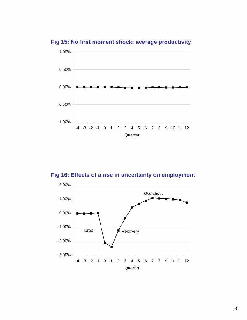
This section motivates the choice of parameter values used in the simulations (see Table 2)

and also presents simulation results for our preferred speci�cation.

22Assuming � > 1 would require the forecasting of an additional function in step 1 above. This wouldsubstantially complicate the numerical solution.

23For the forecasting functions, we use the �rst moments of the distribution over capital and labor as well asthe aggregate uncertainty state. Interestingly, this provides a very good �t and an R2 of above 0.99.

24For the forecasting functions, we use the �rst moments of the distribution over capital and labor as well asthe aggregate uncertainty state. Interestingly, this provides a very good �t and an R2 of above 0.99.

13

4.1 Calibration

4.1.1 Frequency and Preferences

We set the time period to equal a quarter. The household�s discount rate, �, is calibrated

to 0:985, while � is set equal to one implying that the momentary utility function features

an elasticity of intertemporal substitution of one. As discussed above, we assume an in�nite

Frisch labor supply elasticity, or indivisible labor, corresponding to � = 1. We set the

parameter � such that households spend a third of their time working in the non-stochastic

steady state. The trend growth rate of per capita output is set to equal 1:6% annually.

4.1.2 Production Function, Depreciation, and Adjustment Costs

The capital depreciation rate is set to match the average annual depreciation rate of 10%,

leading us to set �k = 0:025. The annual exogenous quit rate of labor is a key parameter,

and is set to 15%. This estimate is based on the quit rate reported in the Bureau of Labor

Statistic JOLTS data.25

We set the �rm�s production function elasticity with respect to its capital stock, � = 0:25

and � = 0:5, consistent with a capital cost share of 1=3 and a 25% markup when the �rm

faces an iso-elastic demand curve.

The existing literature provides a wide range of estimates for capital and labor adjust-

ment costs.26 We set our adjustment cost parameters to match Bloom (2009), which is the

only paper we are aware of that jointly estimates capital and labor convex and non-convex

adjustment costs. Fixed costs of capital adjustment are set to 1:5% of annual sales, and the

resale loss of capital amounts to 40%. The �xed cost of adjusting hours, is set to 2:1% of

annual wages, and the hiring and �ring costs equal 1.8% of annual wages.

4.1.3 Aggregate and Idiosyncratic TFP Processes

We approximate the autoregressive processes (2) and (3) with Markov chains. The supports

for the processes are set to include three standard deviations on either side of the mean.

For idiosyncratic TFP, we increase this range to three times the standard deviation on

either side. The parameters of the processes are taken from Khan and Thomas (2008) and

25JOLTS stands for Job Openings and Labor Turnover Data, which the BLS has been collecting since January2001. Hence, this data spans two NBER de�ned recessions. It distinguishes between quits, layo¤s, and otherseparations. Our �gures are seasonally adjusted for total private employment. In JOLTS, the monthly quit�gure varies between 1:6% and 2:4%, with the lowest value occurring in November 2008 during the depthsof the 2008 recession. Annualizing the November 2008 quit rate we get a value of 19:2%. Our calibrationusing a lower value of 15% is thus a conservative calibration.

26See, for example, Hayashi (1982), Nickel (1986), Shapiro (1986), Caballero and Engel (1999), Ramey andShapiro (2001), Hall (2004), Cooper, Haltiwanger and Willis (2004), Cooper and Haltiwanger (2006) as wellas Mertz and Yashiv (2007).

14

adjusted to the quarterly frequency. Hence, �A and �Z are set to yield an annual persistence

parameter of 0:859, whereas the standard deviation of innovations to the aggregate and

idiosyncratic productivity process are set to yield an annual equivalent of 0.014 and 0.022,

respectively.

4.1.4 The Calibrated Process for Uncertainty

We assume for simplicity that the stochastic volatility processes �At and �Zt follow two-point

Markov chains. In the benchmark calibration we assume that the values of aggregate and

idiosyncratic uncertainty are driven by just one exogenous process that determines whether

the economy is in the normal or uncertain regime. Moreover, in the benchmark calibration,

the uncertainty process is assumed to be completely independent of the �rst-moment shocks.

This implies that we are not arti�cially creating the drop in economic activity following a

second-moment shock by correlating it with the �rst-moment shock.

The stochastic process of uncertainty in the model is only indirectly related to the

uncertainty index we have created in Section 2. Therefore, we proceed by disciplining our

uncertainty process. The model generates a time series for the IQR of cross-�rm sales

growth rates and the IQR of cross-�rms stock returns which are observed in the data. We

thus calibrate the uncertainty process such that the serial autocorrelation and the variance

of the mean of those processes match their observable counterparts in the data. By setting

the increase of �At and �Zt in the high uncertainty state to a factor of 2:03 and using the

following Markov transition matrix we can match the two aforementioned time series:

normal uncertain

normal 0:956 0:044

uncertain 0:208 0:792

This matrix implies that the economy resides in the low uncertainty state 82% of the time.

4.2 The E¤ects of an Uncertainty Shock

We �rst study the e¤ects of an isolated increase in uncertainty. We simulate many economies

and let each run for 500 periods to initialize the distribution over z; k and n, while forcing all

economies to remain in the low uncertainty state. At period zero, all economies are subject

to an uncertainty shock. That is, agents learn that, starting in period one, the distribution

of productivities fans out.27 The expected duration of the processes is governed by the

transition matrix. This leads to an increase in the dispersion of cross-sectional �rm sales

27The magnitude of the shock is such that the standard deviation of the innovations to idiosyncratic andaggregate productivity increase by factors slightly larger than two as outlined in the calibration.

15

growth rates and stock returns of about 25%, matching the real data discussed in Section

2.

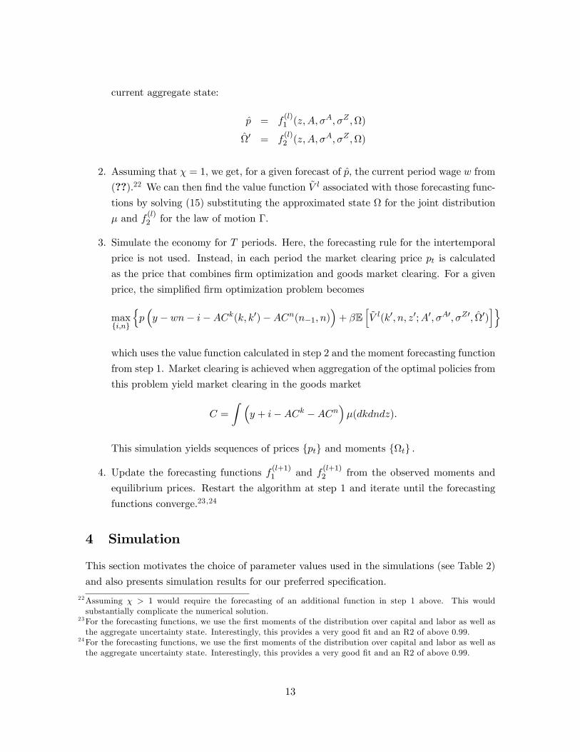
Figure 14 plots the fraction of economies that are in the high uncertainty state in

each quarter, while Figure 15 show that the average �rm productivity does not change

in this experiment. Thus, the baseline simulation results are driven entirely by changes

in uncertainty. In what follows we report the behavior of the variables of interest as the

average over these economies.

The time pro�le of hours worked is shown in Figure 16. In period zero, once uncertainty

rises, �rms defer most hiring decisions, leading to a fall of about 2% in hours worked. Hours

continue to fall until quarter three, by when uncertainty falls enough and productivity fans

out su¢ ciently so that �rms with high productivity draws start to increase hours. By

quarter �ve, the economy has reverted back to the initial trend.

Labor use actually rises above its long-run value for a few more quarters before return-

ing to this long-run level. The reason for such overshooting is that within the economy,

many �rms are bunched near the hiring threshold due to labor attrition. Small increases

in productivity will cause �rms to hire more workers, while small decreases in produc-

tivity will simply move them towards the interior of their (S; s) bands. As a result, the

increased variance of the productivity shock induced by higher uncertainty increases aggre-

gate medium-run hiring. Firms that have received positive productivity shocks hit their

(S; s) bands and hire. Firms that receive a negative shock move to the interior of the (S; s)

bands and do nothing. Since at period zero each �rm�s capital stock is given, the fall in

aggregate hours worked manifests itself into a drop in aggregate output, as can be seen in

Figure 17. Overall, output falls recovers by the fourth quarter and follows the overshooting

of labor. Inter

The uncertainty shock also induces a drop and subsequent rebound in investment, as

shown in Figure 18. As uncertainty rises in period zero, investment expenditure sharply

falls due to postponed investment decisions. Substantial capital adjustment costs lead many

�rms to defer new investment expenditure until after uncertainty has subsided. Investment

recovers by the third quarter as uncertainty has fallen su¢ ciently enough to lead �rms start

to addressing their pent-up demand for investment.

Figure 19 plots the time pro�le of consumption. When the uncertainty shock occurs in

period zero, consumption jumps up immediately and then falls below trend for about �ve

quarters. The reason for the initial spike in consumption is that the freeze in investment

and hiring reduces the resources spent on capital and labor adjustment. Since the interest

rate drops upon impact of the shock, consumers are signaled that consumption is cheap,

which leads to an increase in consumption in period zero. In other words, even though

consumers know they face higher uncertainty in the future and they would like to save

16

more, they do not increase savings in the �rst period because the returns to saving have

become (temporarily) low and very risky.28

Finally, Figure 20 plots the value for the aggregate Solow residual, de�ned as Yt=K�t N

�t .

The Solow residual also has a clear drop and subsequent rebound after the uncertainty

shock, despite the fact that the average micro and macro productivity shocks were un-

changed, as shown in Figure 15. The reason is that uncertainty freezes the reallocation

of capital and labor from low- to high-productivity �rms. In normal times, unproductive

�rms contract and productive �rms expand, helping to maintain high productivity lev-

els. When uncertainty is high, �rms reduce expansion and contraction, shutting o¤ much

of this productivity-enhancing reallocation, leading to a fall in productivity growth rates.

When uncertainty reverts back to normal, �rms rapidly address their pent-up demand for

reallocation so that productivity returns to its long-run trend.

Therefore, a second-moment shock induces a fall in investment, hours, and output.

Intriguingly, the Solow residual also falls even though this is an e¤ect rather than a cause of

the drop in economic activity. Consumption also exhibits a fall from quarter two onwards,

although there is an initial one-period jump in the basic model.

4.3 Model Simulations

We have shown that our model can generate expansions and contractions in response to

an increase in uncertainty. One natural question is whether this success comes at a cost of

the model�s ability to generate empirically recognizable business �uctuations. That is, can

the model, when calibrated with the same parameters used in the experiments discussed so

far, generate co-movement, and volatility of macroeconomic aggregates that are empirically

plausible? To answer this question, we simulate our model and compute the standard set

of business cycle statistics.

As Panel A in Table 3 reports, the benchmark calibration generates second-moment

statistics that closely match the empirical counterparts in the U.S. data. Investment is more

volatile than output, while consumption is less volatile. Investment and hours commove with

output. Similarly to many variants of the RBC model, hours are not as volatile relative to

output as in the data.

28This logic suggests that if we extended the model to allow for some alternative savings technology � forexample, inventories or savings abroad �this initial spike in consumption would disappear as the represen-tative consumer would just increase savings through this channel when the uncertainty shock hit to reducethe subsequent drop in consumption. Due to computational constraints we cannot increase the state spaceof the model.

17

4.4 Robustness Checks

To highlight the role of the adjustment costs in generating the e¤ects of uncertainty shocks as

those reported in Figures 15-20, we depict in Figures 21 and 22 the impact of an uncertainty

when (i) there are only capital adjustment costs (Figure 21), and (ii) when there are no

adjustment costs at all.

As Figure 21 shows, when the uncertainty shocks hits the economy and there are only

capital adjustment costs output does not react. This is not surprising as on impact capital

is a state variable and hence labor does not react. Since at period zero investment falls,

starting in period 1 capital falls as hence output falls below trend and later recovers. Figure

22 shows that when there are no adjustment costs of any type in the economy, economic

activity actually increases following an uncertainty shock. The reason for this result is

related to the Hartman-Abel e¤ect. 29

4.5 Uncertainty Shocks as a Magni�cation Mechanism

We have assumed so far that the uncertainty process is completely independent of the

�rst-moment shocks. In this subsection we relax this assumption.

[To be completed].

5 Policy in the Presence of Uncertainty

In this section, we analyze the e¤ects of a policy that tries to increase investment in an

economy that is faced with shocks to uncertainty. As we argue below, uncertainty widens

�rms�(S; s) bands for investment and hiring, thereby reducing the impact response of any

given policy. Figure 23 plots the evolution of the cross-sectional distribution of the ratio

of �rm TFP to capital in the model.30 The uncertainty shock occurs in period zero. Note

how, on impact, the investment and disinvestment threshold fan out. Slowly over time, as

�rms begin drawing their new high (low) productivity shocks, the distribution of �rm-level

TFP fans out towards the thresholds. For example, assume that a normal policy moves the

threshold downward by 5%. Such a policy would have pushed about 50% of the �rms over

the investment threshold in normal times (i.e. periods -4,-3,-2,-1). But, the same policy

29Panles B-F in Table 3 resport the second-moment statistics for di¤ernet robustness checks relative to thebenchmark model. Speci�cally, we consider �ve robustness checks: (i) No adjustment costs of any type (PanelB), (ii) only macro uncertainty (Panel C), (iii) only micro uncertainty (Panel D), (iv) a high dispersion ofmacro shocks relative to micro shocks (Panel E), and (v) a high dispersion of micro shocks relative to macroshocks (Panel F). As Table 3 shows, the second-moment statistics in all of these experiemnts closely resemblethose in Panel A. This similarity is not surprising as all of these economies are subject to the �rst-momentshocks.

30 In order to be able to draw the distribution, we look at the values of TFP/k for given capital and laborvalues.

18

would have had zero impact time zero, when the uncertainty shock occurs, since such a

move in the threshold would have no e¤ect on �rms!

To substantiate these claims, we conduct a policy experiment. Speci�cally, we analyze

the case of a 1% surprise investment credit for one quarter and we evaluate its e¤ect during

a normal period and after an uncertainty shock.31 ;32 Figure 24 shows the response of output

to such a policy, that takes place at period zero in two cases. The line with squares shows

the response of output to such a policy in the case of low uncertainty. The line with triangles

shows the behavior of output in response to an uncertainty shock, while the line with circles

shows the response of this economy with a tax credit. The di¤erence between the second and

the third line is the impact of policy during high uncertainty times. Figure 25, shows the

di¤erential e¤ects of the policy in the two economies (line 1 versus the di¤erence between

lines 2 and 3 from Figure 24). As is clear from the �gure, the presence of uncertainty

mitigates the e¤ects of such a policy relative to an economy that is in the normal, or low

uncertainty, state.

Two messages that arise from this experiment are that in order for such a policy to have

any e¤ect on investment in the presence of uncertainty, it has to be both larger (in order

to move the investment threshold down) and shorter-lived (in order to avoid overshooting

once uncertainty falls) than the policy that would be implemented during normal times.

6 Conclusions

This paper proposes time variation in uncertainty as an additional impulse driving business

cycles. First, we demonstrate that uncertainty, measured by a number of proxies, appears

to be strongly countercyclical. When added to a standard VAR, increases in uncertainty

lead to a large drop and subsequent rebound in economic activity. This result holds even

after controlling for �rst-moment e¤ects.

Second, we study a dynamic stochastic general equilibrium model that allows for shocks

to both the level of technology (the �rst moment) as well as uncertainty (the second mo-

ment). More speci�cally, we model shocks to uncertainty as variation in the standard

deviation of the innovations to productivity. We �nd that increases in uncertainty lead to

large drops in employment and investment. This occurs because uncertainty makes �rms

cautious, leading them to pause hiring and investment. This freezing in activity also re-

duces the reallocation of capital and labor across �rms, leading to a large fall in productivity

31We assume this credit comes "from Mars" and abstract from general equilibrium balanced budget consider-ations.

32Note that this tax credit is not optimal. The optimal policy is to do exactly nothing in this setup. We arethus analyzing this policy experiment merely as a way to summarize the potential e¤ects of policy in thepresence of uncertainty.

19

growth. Taken together, the freeze in hiring, investment and productivity growth leads to

a business-cycle-sized drop and rebound in output following a rise in uncertainty.

We then conclude by using our model to investigate the e¤ects of uncertainty on pol-

icy e¤ectiveness. We use a simple illustrative example to show the presence signi�cantly

dampens the e¤ect of an expansionary policy.

20

References

Abel, A.B. and Eberly, J.C. (1996), "Optimal Investment with Costly Reversibility", Review ofEconomic Studies, 63(4), 581-593.

Abraham, K.G. and Katz, L.F. (1986), "Cyclical Unemployment: Sectoral Shifts or Aggregate Dis-turbances?", Journal of Political Economy, 9(3), 507-522.

Aghion, P., Angeletos, G., Banerjee, A. and Manova, K. (2005), "Volatility and Growth: CreditConstraints and Productivity-Enhancing Investment", NBER WP 11349.

Amador, M. and Weill, P.-O. (2008), "Learning from Private and Public Observations of Others�Actions", Stanford mimeo.

Bachman, R., Caballero, R.J. and Engel, E.M.R.A. (2008), "Aggregate Implications of Lumpy In-vestment: New Evidence and a DSGE Model", Yale mimeo.

Bartelsman, E., Becker, R. and Gray, W. (2000), "NBER Productivity Database", www.nber.org.

Barlevy, G. (2004), "The Cost of Business Cycles Under Endogenous Growth", American EconomicReview, 94(4), 964-990.

Basu, S., Fernald, J. and Kimball, M.S. (2006), "Are Technology Improvements Contractionary?",American Economic Review, 96(5), 1418-1448.

Bernanke, B. (1983), "Irreversibility, Uncertainty and Cyclical Investment", Quarterly Journal ofEconomics, 98, 85-106.

Bentolila, S. and Bertola, G. (1990), "Firing Costs and Labor Demand: How Bad is Eurosclerosis",Review of Economic Studies, 57(3), 381-402.

Bernard, A., Redding, S. and Schott, P. (2006), "Multi-Product Firms and Product Switching",NBER WP 12293.

Bertola, G. and Caballero, R.J. (1994), "Irreversibility and Aggregate Investment", Review of Eco-nomic Studies, 61, 223-246.

Bloom, N. (2009), "The Impact of Uncertainty Shocks", forthcoming Econometrica.

Bloom, N. (2007), "Uncertainty and the Dynamics of R&D", American Economic Review Papersand Proceedings, 97(2), 250-255.

Bomberger, W. A. (1996), "Disagreement as a Measure of Uncertainty", Journal of Money, Creditand Banking, 28(3), 381-392.

Caballero, R.J. and Engel, E.M.R.A (1999),"Explaining Investment Dynamics in U.S. Manufactur-ing: a Generalized (S,s) Approach", Econometrica, 67(4), 783-826.

Caballero, R.J. and Leahy, J. (1996), "Fixed costs: the demise of marginal Q", NBER WP 5508.

Campbell, J., Lettau, M., Malkiel B. and Xu, Y. (2001), "Have Individual Stocks Become MoreVolatile? An Empirical Exploration of Idiosyncratic Risk", Journal of Finance, 56(1), 1-43.

Christiano, L.J., Eichenbaum, M. and Evans, C.L. (2005), "Nominal Rigidities and the DynamicE¤ects of a Shock to Monetary Policy", Journal of Political Economy, 113(1), 1-45.

21

Davis, S.J. and Haltiwanger, J. (1992), "Gross Job Creation, Gross Job Destruction, and Employ-ment Reallocation�, Quarterly Journal of Economics, 107, 819-863.

Davis, S.J., Haltiwanger, J., Jarmin, R. and Miranda, J. (2006), "Volatility and Dispersion inBusiness Growth Rates: Publicly Traded Versus Privately Held Firms", NBER WP 12354.

Dixit, A.K. and Pindyck, R.S. (1994), "Investment Under Uncertainty", Princeton University Press,Princeton.

Engle, R.F. and Rangel, J.G. (2008), "The Spline-GARCH Model for Low-Frequency Volatility andIts Global Macroeconomic Causes", Review of Financial Studies, 21(3), 1187-1222.

Faggio, G., Salvanes K.G. and Van Reenen, J. (2007), �Understanding Wage and ProductivityDispersion in the United Kingdom", mimeo.

Foster, L., Haltiwanger, J. and Krizan, C.J. (2000), "Aggregate Productivity Growth: Lessonsfrom Microeconomic Evidence", New Developments in Productivity Analysis, NBER, University ofChicago Press.

Foster, L., Haltiwanger, J. and Krizan, C.J. (2006), "Market Selection, Reallocation and Restruc-turing in the U.S. Retail: Trade Sector in the 1990s", Review of Economics and Statistics, 88,748-758.

Koren, M. and Tenreyro, S. (2007), "Volatility and Development", Quarterly Journal of Economics,122(1), 243-287.

Gilchrist, S. and Williams, J.C. (2005), "Investment, Capacity, and Uncertainty: A Putty-ClayApproach", Review of Economic Dynamics, 8(1), 1-27.

Giordani,P. and Soderlind, P (2004), "In�ation Forecast Uncertainty", European Economic Review,47(6), 1037-1059.

Hall, R.E. (2004), "Measuring Factor Adjustment Costs", Quarterly Journal of Economics, 119,899-927.

Hamilton, J.D. and Lin, G. (1996), "Stock Market Volatility and the Business Cycle", Journal ofApplied Econometrics, 11(5), 573-593.

Hammermesh, D. (1989), "Labor demand and the structure of adjustment costs", American Eco-nomic Review, 79, 674-89.

Hassler, J. (1996), "Variations in Risk and Fluctuations in Demand - a Theoretical Model", Journalof Economic Dynamics and Control, 20, 1115-1143.

House, C.L. (2008), "Fixed Costs and Long-Lived Investments", NBER WP 14402.

Jaimovich, N. and Siu, H. (2008), "The Young, the Old, and the Restless: Demographics andBusiness Cycle Volatility", forthcoming American Economic Review.

Keynes, J.M. (1936), "The General Theory of Empployment, Interest and Money", Macmillan,London.

Lillien, D.M. (1982), "Sectoral Shifts and Cyclical Unemployment", Journal of Political Economy,90(4), 777-793.

22

Khan, A. and Thomas, J.K. (2003), "Nonconvex Factor Adjustments in Equilibrium Business CycleModels: Do Nonlinearities Matter?", Journal of Monetary Economics, 50, 331-360.

Khan, A. and Thomas, J.K. (2008), "Idiosyncratic Shocks and the Role of Nonconvexities in Plantand Aggregate Investment Dynamics, Econometrica, 76(2), 395-436.

King, R.G. and Rebelo, S.T. (1999), "Resuscitating Real Business Cycles", in Handbook of Macro-economics, John B. Taylor and Michael Woodford (eds.), Elsevier.

Krusell, P and Smith, A.A. (1998), "Income and Wealth Heterogeneity in the Macroeconomy",Journal of Political Economy, 106(5), 867-896.

Mele, A. (2007), "Asymmetric Stock Market Volatility and the Cyclical Behavior of Expected Re-turns", Journal of Financial Economics, 86, 446-478.

Merz, M. and Yashiv, E. (2007), "Labor and the Market Value of the Firm", American EconomicReview, 97(4), 1419-1431.

Nickell, S.J. (1986), "Dynamic Models of Labor Demand", in O. Ashenfelter and R. Layard (eds.),Handbook of Labor Economics, North-Holland, Amsterdam.

O¢ cer, R. (1973), "The Variability of the Market Factor of the New York Stock Exchange", Journalof Business, 46, 434-453.

Pindyck, R.S. (1988), "Irreversible Investment, Capacity Choice, and the Value of the Firm", Amer-ican Economic Review, 78(5), 969-985.

Ramey, V.A. and Ramey, G. (1994),"Cross-Country Evidence on the Link between Volatility andGrowth", American Economic Review, 85, 1138-1151.

Ramey, V.A. and Shapiro, M.D. (2001) "Displaced Capital: A Study of Aerospace Plant Closings",Journal of Political Economy, 109, 605-622.

Rebelo, S.T. (2005), "Real Business Cycle Models: Past, Present, and Future", Scandinavian Journalof Economics, 107(2), 217-238.

Schwert, G.W. (1989), "Why Does Stock Market Volatility Change Over Time?", Journal of Finance,44, 1115�1153.

Storesletten, K., Telmer, C.I. and Yaron, A. (2004), "Cyclical Dynamics in Idiosyncratic Labor-Market Risk", Journal of Political Economy, 112(3), 695-717.

Thomas, J.K. (2002), "Is Lumpy Investment Relevant for the Business Cycle?", Journal of PoliticalEconomy, 110(3), 508-534.

Veracierto, M.L. (2002),"Plant Level Irreversible Investment and Equilibrium Business Cycles",American Economic Review, 92(1), 181-197.

Zarnowitz, V. and Lambros, L.A. (1987), "Consensus and Uncertainty in Economic Prediction",Journal of Political Economy, 95(3), 591-621.

23

A Appendix: Uncertainty Data

To be added.

B Appendix: Numerical Solution Method

To be added.

24

1

Fig 1: Cross firm sales growth spread

Interquartile range of sales growth (Compustat firms). Only firms with 25+ years of accounts, and quarters with 500+ observations. SIC2 only cells with 25+ obs.

.2.3

.4.5

1970 1980 1990 2000 2010Year

Across all firms(+ symbol)

Across firms in a SIC2 industry

Fig 2: Cross firm sales growth spread

Interquartile range of sales growth (Compustat firms). Only firms with 25+ years of accounts, and quarters with 500+ observations. SIC2 only cells with 25+ obs.

.2.3

.4.5

1970 1980 1990 2000 2010Year

Normal series (in blue)Residuals from firm level regressions of growth on recessions (in green)

2

Interquartile range of stock returns (CRSP firms). Only firms with 25+ years of accounts, and quarters with 500+ observations. SIC2 only cells with 25+ obs.

Fig 3: Cross firm stock returns spread

.05

.1.1

5.2

1970 1980 1990 2000 2010Year

Across all firms(+ symbol)

Across firms in a SIC2 industry

Interquartile range of stock returns (CRSP firms). Only firms with 25+ years of accounts, and quarters with 500+ observations. SIC2 only cells with 25+ obs.

Fig 4: Cross firm stock returns spread

.05

.1.1

5.2

1970 1980 1990 2000 2010Year

Residuals from firm level regressions of growth on recessions (in green)

Normal series (in blue)

3

Inter-quartile range of the 3-month growth rates of industrial production. Covers all 196 manufacturing NAICS sectors in the Federal Reserve Board database.

Fig 5: Cross industry output growth spread

.01

.02

.03

.04

.05

.06

1970 1980 1990 2000 2010Year

Residuals from industrylevel regressions of growth on recessions (in green)

Normal series (in blue)-.4

-.20

.2

1970 1980 1990 2000 2010Year

1st, 5th, 10th, 25th, 50th, 75th, 90th, 95th and 99th percentiles of 3-month growth rates of industrial production within each quarter. All 196 manufacturing NAICS sectors in the Federal Reserve Board database.

99th percentile,2.2% higher in recessions

1st percentile7.4% lower in recessions

50th percentile,1.3% lower in recessions

Fig 6: Cross industry output growth distribution

4

Monthly industrial production conditional heteroskedasticity, from a GARCH(1,1) auto-regression with 12 lags.

.005

.01

.015

.02

.025

1965 1970 1975 1980 1985 1990 1995 2000 2005Year

Fig 7: Industrial production growth volatility

1020

3040

5060

1965 1970 1975 1980 1985 1990 1995 2000 2005Year

Fig 8: Stock market volatility

S&P 100 implied volatility (the VXO, which is very similar to VIX) from 1987, and normalized realized volatility of actual S&P100 daily stock returns prior to 1986.

5

Interquartile range of year ahead unemployment rates / mean unemployment rates. From Survey of Professional Forecasters. Average of 41 forecasts per quarter.

Fig 9: Forecaster dispersion for unemployment

0.0

5.1

.15

.2

1970 1975 1980 1985 1990 1995 2000 2005Year



Fig 10: Forecaster dispersion for ind production

Interquartile range of year ahead production/mean production. From Survey of Professional Forecasters. Average of 41 forecasts per quarter.

0.0

2.0

4.0

6

1970 1975 1980 1985 1990 1995 2000 2005Year



6

.51

1.5

22.

5

1965 1970 1975 1980 1985 1990 1995 2000 2005Year

Fig 11: Uncertainty index

Mean of the 7 prior indicators after they have all been normalized to an average of 1 during non-recessionary quarters. Only reported when 6+ indicators present.

Fig 12: VAR analysis – uncertainty firstShock calibrated to increase uncertainty 48% during recessions

Cholesky orthogonalized on quarterly data from 1968:4 to 2006:4 using 4 lags. Dotted lines are 95% confidence intervals

7

Fig 13: VAR analysis – different experiments

Cholesky orthogonalized on quarterly data from 1968:4 to 2006:4 using 4 lags. Dotted lines are 95% confidence intervals

Shock calibrated to increase uncertainty 48% during recessions

Fig 14: % of economies in the high uncertainty state

0%10%

20%

30%

40%

50%

60%

70%

80%

90%

100%

-4 -3 -2 -1 0 1 2 3 4 5 6 7 8 9 10 11 12

Quarter

8

Fig 15: No first moment shock: average productivity

-1.00%

-0.50%

0.00%

0.50%

1.00%

-4 -3 -2 -1 0 1 2 3 4 5 6 7 8 9 10 11 12

Quarter

Fig 16: Effects of a rise in uncertainty on employment

-3.00%

-2.00%

-1.00%

0.00%

1.00%

2.00%

-4 -3 -2 -1 0 1 2 3 4 5 6 7 8 9 10 11 12

Quarter

Drop Recovery

Overshoot

9

Fig 17: Effects of a rise in uncertainty on output

-3.00%

-2.00%

-1.00%

0.00%

1.00%

2.00%

-4 -3 -2 -1 0 1 2 3 4 5 6 7 8 9 10 11 12

Quarter

Fig 18: Effects of a rise in uncertainty on investment

-45.00%

-35.00%

-25.00%

-15.00%

-5.00%

5.00%

15.00%

25.00%

35.00%

-4 -3 -2 -1 0 1 2 3 4 5 6 7 8 9 10 11 12

Quarter

10

Fig 19: Effects of a rise in uncertainty on consumption

-5.00%

-4.00%

-3.00%

-2.00%

-1.00%

0.00%

1.00%

2.00%

3.00%

4.00%

-4 -3 -2 -1 0 1 2 3 4 5 6 7 8 9 10 11 12

Quarter

Fig 20: Effects of a rise in uncertainty on TFP

-1.00%

-0.50%

0.00%

0.50%

1.00%

-4 -3 -2 -1 0 1 2 3 4 5 6 7 8 9 10 11 12

Quarter

11

Fig 21: Only K AC: Output response to an uncertainty shock

-2.50%

-2.00%

-1.50%

-1.00%

-0.50%

0.00%

0.50%

1.00%

1.50%

-4 -3 -2 -1 0 1 2 3 4 5 6 7 8 9 10 11 12Quarter

Only K AC

Benchmark model

Fig 22: Effects of a rise in uncertainty: No AC

Labor

-0.20%

0.00%

0.20%

0.40%

0.60%

0.80%

1.00%

1.20%

1.40%

-4 -3 -2 -1 0 1 2 3 4 5 6 7 8 9 10 11 12

Quarter

Output

-0.20%

0.00%

0.20%

0.40%

0.60%

0.80%

1.00%

1.20%

1.40%

-4 -3 -2 -1 0 1 2 3 4 5 6 7 8 9 10 11 12

Quarter

Investment

-15.00%-10.00%-5.00%0.00%5.00%

10.00%15.00%20.00%25.00%30.00%

-3 -2 -1 0 1 2 3 4 5 6 7 8 9 10 11 12

Quarter

12

0.80

0.85

0.90

0.95

1.00

1.05

1.10

1.15

-4 -3 -2 -1 0 1 2 3 4 5 6 7 8 9 10

Quarter

Investment threshold

Disinvestment threshold

90th

10th

50th

Fig 23: Cross-sectional distribution of firm TFP/capital

Thresholds & percentiles of firm distribution over z (for fixed k & l)

Fig 24: Impact of 1% investment credit

-3.00%

-2.00%

-1.00%

0.00%

1.00%

2.00%

3.00%

4.00%

5.00%

-4 -3 -2 -1 0 1 2 3 4 5 6 7 8 9 10 11 12

Quarter

Uncertainty shock without policy response

Investment credit + low uncertainty

Uncertainty shock with investment credit

13

Fig 25: Impact of 1% investment credit

-3.00%

-2.00%

-1.00%

0.00%

1.00%

2.00%

3.00%

4.00%

5.00%

-4 -3 -2 -1 0 1 2 3 4 5 6 7 8 9 10 11 12

Quarter

Investment credit + low uncertainty

Impact of investment credit during uncertainty shock

Table 1: The Increase in Measures of Uncertainty During Recessions% increase during recessions, correlation with quart. period coveredmean (standard deviation) ind. production growth

(1) Firm sales growth spread 23.1 (3.4) -0.471 67Q2 to 08Q2(quarterly cross-sectional interquartile range)

(2) Firm stock returns spread 22.4 (3.6) -0.367 69Q1 to 08Q4(quarterly cross-sectional interquartile range)

(3) Industry output growth spread 66.5 (5.4) -0.603 72Q1 to 09Q1(quarterly cross-sectional interquartile range)

(4) Macro output growth volatility 57.6 (13.1) -0.409 62Q1 to 09Q1(quarterly average conditional standard deviation)

(5) Macro stock returns volatility 44.2 (6.8) -0.470 63Q1 to 09Q2(quarterly standard deviation of daily stock returns)

(6) Forecaster predicted industrial production spread 62.5 (9.3) -0.282 68Q4 to 09Q2(quarterly interquartile range / mean)

(7) Forecaster predicted unemployment spread 70.4 (6.9) -0.535 68Q4 to 09Q2(quarterly interquartile range / mean)

(8) Uncertainty index 47.3 (3.6) -0.621 68Q4 to 08Q4(average of normalized individual measures)

Table 1: Uncertainty and the Recession

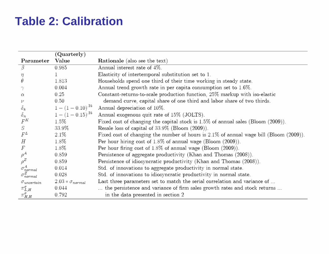
Table 2: Calibration

SD(X) SD/SD(Y) Corr(X,Y)Y 1.80 1.00 1.00I 9.54 5.30 0.87C 1.04 0.58 0.56N 1.24 0.69 0.97

Benchmark ModelSD(X) SD/SD(Y) Corr(X,Y)

Y 1.80 1.00 1.00I 9.18 5.10 0.89C 0.95 0.53 0.60N 1.21 0.67 0.96

NO AC


Only Macro UNCSD(X) SD/SD(Y) Corr(X,Y)

Y 1.60 1.00 1.00I 7.84 4.90 0.82C 1.07 0.67 0.61N 1.02 0.64 0.97

Only Micro UNC


High Macro DispersionSD(X) SD/SD(Y) Corr(X,Y)

Y 1.80 1.00 1.00I 8.82 4.90 0.72C 0.79 0.44 0.43N 1.26 0.70 0.96

High Micro Dispersion

Table 3: Second moment statistics

Panel A Panel B

Panel C

Panel E Panel F

Panel D

Really Uncertain Business Cycles

Documents