Reality conditions and Ashtekar variables: A different perspective

arX

iv:g

r-qc

/941

0013

v1 1

1 O

ct 1

994

CGPG-94/10-2

Reality Conditions and Ashtekar Variables: a Different

Perspective

J. Fernando Barbero G. ∗,†

∗Center for Gravitational Physics and GeometryDepartment of Physics,

Pennsylvania State University,University Park, PA 16802

U.S.A.†Instituto de Matematicas y Fısica Fundamental,

C.S.I.C.Serrano 119–123, 28006 Madrid, Spain

October 10, 1994

ABSTRACT

We give in this paper a modified self-dual action that leads to the SO(3)-ADMformalism without having to face the difficult second class constraints present inother approaches (for example, if one starts from the Hilbert-Palatini action). Weuse the new action principle to gain some new insights into the problem of the realityconditions that must be imposed in order to get real formulations from complexgeneral relativity. We derive also a real formulation for Lorentzian general relativityin the Ashtekar phase space by using the modified action presented in the paper.PACS numbers: 04.20.Cv, 04.20.Fy

I Introduction

The purpose of this paper is to present a modified form of the self-dual action and use

it to discuss the problem of reality conditions in the Ashtekar description of general

relativity. By now, the Ashtekar formulation [1] has provided us with a new way to

study gravity from a non-perturbative point of view. The success of the program

can be judged from the literature available about it [2]. In our opinion there are two

main technical points that have contributed to this success. The first one is the fact

that the configuration variable is an SO(3) connection. This allows us to formulate

general relativity in the familiar phase space of the Yang-Mills theory for this group.

We can then take advantage of the many results about connections available in the

mathematical physics literature. In particular, it proves to be very useful to have

the possibility of using loop variables [3] (essentially Wilson loops of the Ashtekar

connection and related objects) in both the classical and the quantum descriptions of

the theory. A second important feature of the Ashtekar formalism is the fact that the

constraints (in particular the Hamiltonian constraint) have a very simple structure

when written in terms of the new variables. This has been very helpful in order to

find solutions to all the constraints of the theory and is in marked contrast with the

situation in the ADM formalism [4] where the scalar constraint is very difficult to

work with because of its rather complicated structure.

In spite of all the success of the formulation, there are still several problems that

the Ashtekar program has to face. The one that we will be mostly concerned with

in this paper is the issue of the reality conditions. As it is well known, the so called

reality conditions must be imposed on the complex Ashtekar variables in order to

recover the usual real formulation of general relativity for space-times with Lorentzian

signatures. Their role is to guarantee that both the three-dimensional metric and its

time derivative (evolution under the action of the Hamiltonian constraint) are real.

This introduces key difficulties in the formulation, specially when one tries to work

1

with loop variables (although some progress on this issue has been recently reported

[5]).

The main purpose of this paper is to clarify some issues related with the real for-

mulations of general relativity that can be obtained from a given complex theory. We

will see, for example, that both in the1 SO(3)-ADM and in the Ashtekar phase space

it is possible to find Hamiltonian constraints that trivialize the reality conditions to

be imposed on the complex theory (regardless of the signature of the space-time).

Conversely, any of this alternative forms for the constraints in a given phase space

can be used to describe Euclidean or Lorentzian space-times, provided that we im-

pose suitable reality conditions. Though this fact is, somehow, obvious in the ADM

framework, it is not so in the Ashtekar formalism. In doing this we will find a real

formulation for Lorentzian general relativity in the Ashtekar phase space. The main

difference between this formulation and the more familiar one is the form of the scalar

constraint. We will need a complicated expression in order to describe Lorentzian sig-

nature space-times. In our approach, the problem of the reality conditions is, in fact,

transformed into the problem of writing the new Hamiltonian constraint in terms of

loop variables and, in the Dirac quantization scheme, imposing its quantum version

on the wave functionals (issues that will not be addressed in this paper). Of course

one must also face the difficult problems of finding a scalar product in the space of

physical states etc...

A rather convenient way of obtaining the new Hamiltonian constraint is by starting

with a modified version of the usual self-dual action [7] that leads to the SO(3)-

ADM formalism in such a way that the transition to the Ashtekar formulation is very

transparent. We will take advantage of this fact in order to obtain the real Lorentzian

formulation and to discuss the issue of reality conditions.

The lay-out of the paper is as follows. After this introduction we review, in section

1in the following we mean by SO(3)-ADM formalism the version of the ADM formalism in whichan internal SO(3) symmetry group has been introduced as in [9].

2

II, the self-dual action and rewrite it as the Husain-Kuchar [8] action coupled to an

additional field. This will be useful in the rest of the paper. Section III will be devoted

to the modified self-dual action that leads to the SO(3)-ADM formalism. We discuss

the issue of reality conditions in section IV. We will show that although multiplying

the usual self-dual action by a purely imaginary constant factor does not change

anything (both at the level of the field equations and the Hamiltonian formulation),

the same procedure, when used with the modified self-dual action changes the form

of the ADM Hamiltonian constraint (in fact it changes the relative sign between the

kinetic and potential terms that in a real formulation controls the signature of the

space-time). In section V we derive the real Ashtekar formulation for Lorentzian

signatures and we end the paper with our conclusions and comments in section VI.

II The self dual action and Ashtekar variables

We will start by introducing our conventions and notation. Tangent space indices

and SO(3) indices are represented by lowercase Latin letters from the beginning

and the middle of the alphabet respectively. No distinction will be made between

3-dimensional and 4-dimensional tangent space indices (the relevant dimensionality

will be clear from the context). Internal SO(4) indices are represented by capital latin

letters from the middle of the alphabet. The 3-dimensional and 4-dimensional Levi-

Civita tensor densities will be denoted2 by ηabc and ηabcd and the internal Levi-Civita

tensors for both SO(3) and SO(4) represented by ǫijk and ǫIJKL. The tetrads eaI will

be written in components as eaI ≡ (va, eai) (although at this point the i index only

serves the purpose of denoting the last three internal indices of the tetrad we will show

later that it can be taken as an SO(3) index). SO(4) and SO(3) connections will be

denoted by AaIJ and Aai respectively with corresponding curvatures FabIJ and Fabi

given by FabIJ ≡ 2∂[aAb]IJ+A KaI AbKJ−A K

bI AaKJ and F iab ≡ 2∂[aA

ib]+ǫi

jkAjaA

kb . The

2We represent the density weights by the usual convention of using tildes above and below thefields.

3

actions of the covariant derivatives defined by these connections on internal indices

are ∇aλI = ∂aλI + A KaI λK and ∇aλi = ∂aλi + ǫijkAajλk. They can be extended to

act on tangent space indices by introducing a torsion-free connection (for example

the Christoffel connection Γcab built with the four-metric qab ≡ eaIe

Ib). All the results

in the paper will be independent of such an extension. We will work with self-dual

and anti-self-dual objects satisfying B±IJ = ±1

2ǫ KLIJ B±

KL where we raise and lower

SO(4) indices with the internal Euclidean metric Diag(++++). In particular, A−IJ

will be an anti-self-dual SO(4) connection (taking values in the anti-selfdual part of

the complexified Lie algebra of SO(4)) and F−abIJ its curvature. In space-times with

Lorentzian signature a factor i must be included in the definition of self-duality if we

impose the usual requirement that the duality operation be such that its square is the

identity and raise and lower internal indices with the Minkowski metric Diag(−+++).

In this paper we will consider complex actions invariant under complexified SO(4).

For the purpose of performing the 3+1 decomposition the space-time manifold is

restricted to have the form M =lR×Σ with Σ a compact 3-manifold with no boundary.

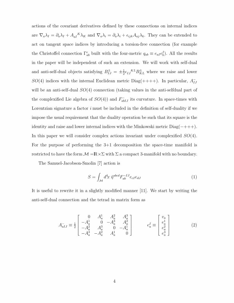
The Samuel-Jacobson-Smolin [7] action is

S =∫

Md4x ηabcdF−IJ

ab ecIedJ (1)

It is useful to rewrite it in a slightly modified manner [11]. We start by writing the

anti-self-dual connection and the tetrad in matrix form as

A−aIJ ≡ 1

2

0 A1a A2

a A3a

−A1a 0 −A3

a A2a

−A2a A3

a 0 −A1a

−A3a −A2

a A1a 0

eIa ≡

va

e1a

e2a

e3a

(2)

4

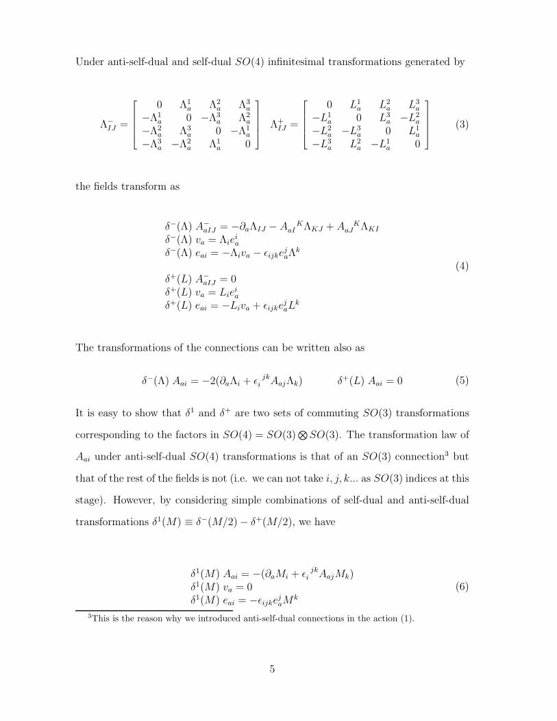
Under anti-self-dual and self-dual SO(4) infinitesimal transformations generated by

Λ−IJ =

0 Λ1a Λ2

a Λ3a

−Λ1a 0 −Λ3

a Λ2a

−Λ2a Λ3

a 0 −Λ1a

−Λ3a −Λ2

a Λ1a 0

Λ+IJ =

0 L1a L2

a L3a

−L1a 0 L3

a −L2a

−L2a −L3

a 0 L1a

−L3a L2

a −L1a 0

(3)

the fields transform as

δ−(Λ) A−aIJ = −∂aΛIJ − A K

aI ΛKJ + A KaJ ΛKI

δ−(Λ) va = Λieia

δ−(Λ) eai = −Λiva − ǫijkejaΛ

k

δ+(L) A−aIJ = 0

δ+(L) va = Lieia

δ+(L) eai = −Liva + ǫijkejaL

k

(4)

The transformations of the connections can be written also as

δ−(Λ) Aai = −2(∂aΛi + ǫ jki AajΛk) δ+(L) Aai = 0 (5)

It is easy to show that δ1 and δ+ are two sets of commuting SO(3) transformations

corresponding to the factors in SO(4) = SO(3)⊗

SO(3). The transformation law of

Aai under anti-self-dual SO(4) transformations is that of an SO(3) connection3 but

that of the rest of the fields is not (i.e. we can not take i, j, k... as SO(3) indices at this

stage). However, by considering simple combinations of self-dual and anti-self-dual

transformations δ1(M) ≡ δ−(M/2) − δ+(M/2), we have

δ1(M) Aai = −(∂aMi + ǫ jki AajMk)

δ1(M) va = 0δ1(M) eai = −ǫijke

jaM

k

(6)

3This is the reason why we introduced anti-self-dual connections in the action (1).

5

As we can see, Aai, eai, va do transform as SO(3) objects under the action of δ1

if we consider the indices i, j, k... as SO(3) indices. The invariance of va under these

transformations makes it very natural to consider the gauge fixing condition va = 0

that we will use later. In terms of Aai, va and eai the action (1) reads

S =∫

Md4xηabcd

[

vaebiFcdi −1

2ǫijkeaiebjFcdk

]

(7)

This form of the Samuel-Jacobson-Smolin action has some nice features. It shows,

for example, that general relativity can be obtained from the Husain-Kuchar [8] model

action by introducing a vector field va and a suitable interaction term. This is useful

in order to study the dynamics of degenerate solutions given by the action (in contrast

with the usual approach of extending the validity of the Ashtekar constraints to the

degenerate sector of the theory). The action (7) will also be the starting point of

the next section in which we show that a certain modification of it gives rise to the

SO(3)−ADM formalism and provides a very natural way of linking it to the Ashtekar

formulation.

The fact that complexified SO(4) and SO(1, 3) coincide means that we can start

from (1), raise and lower indices with the Minkowski metric Diag(−+++) and define

self-dual and anti-self-dual fields by B±IJ = ± i

2ǫ KLIJ B±

KL. It is straightforward to

show that the resulting action is equivalent to (1) because they can be related by

simple redefinitions of the fields.

In the passage to the Hamiltonian formulation 4 corresponding to (7) we introduce

a foliation of the space-time manifold M defined by hypersurfaces of constant value

of a scalar function t. We need also a congruence of curves with tangent vector ta

satisfying ta∂at = 1 (with this last requirement time derivatives can be interpreted as

Lie derivatives Lt along the vector field ta). Performing the 3+1 decomposition we

have

S =∫

dt∫

Σd3x

(LtAia)η

abc[

2vbeci − ǫ jki ebjeck

]

+ Ai0∇a

[

ηabc(2vbeci − ǫ jki ebjeck)

]

+

4We include this short discussion for further reference; the details can be found in [7].

6

+v0ηabcei

aFbci − ei0η

abc[

vaFbci + ǫ jki eajFbck

]

≡∫

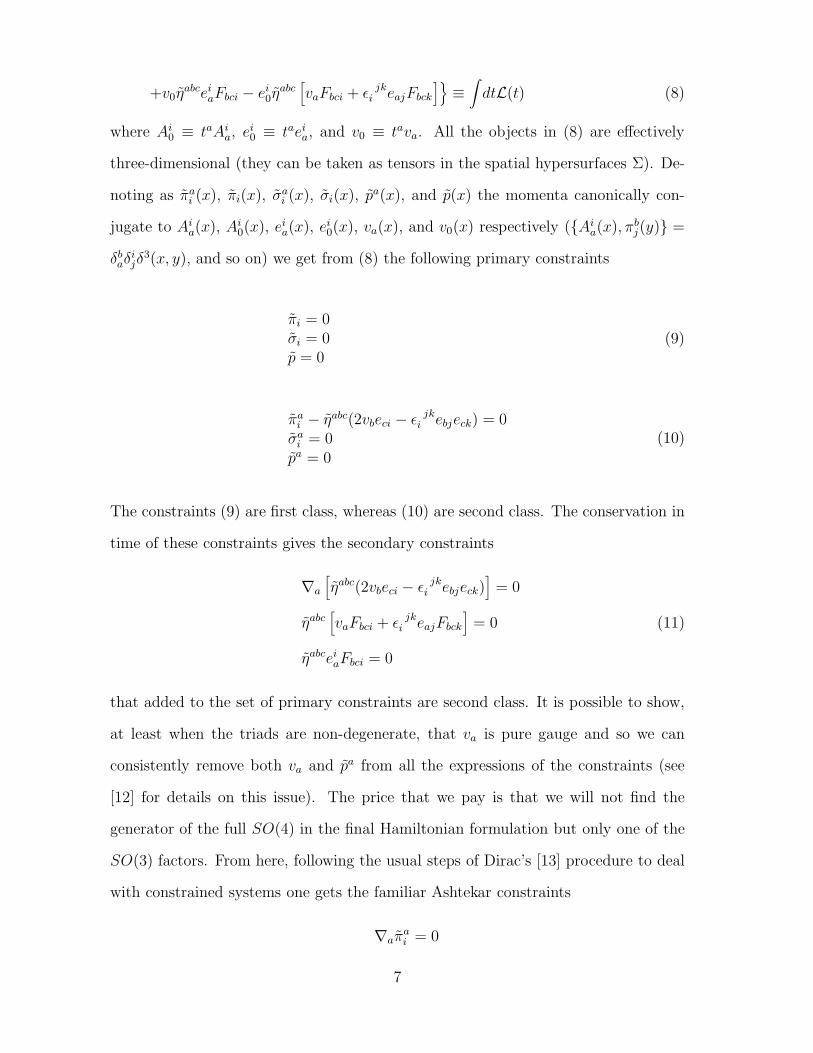
dtL(t) (8)

where Ai0 ≡ taAi

a, ei0 ≡ taei

a, and v0 ≡ tava. All the objects in (8) are effectively

three-dimensional (they can be taken as tensors in the spatial hypersurfaces Σ). De-

noting as πai (x), πi(x), σa

i (x), σi(x), pa(x), and p(x) the momenta canonically con-

jugate to Aia(x), Ai

0(x), eia(x), ei

0(x), va(x), and v0(x) respectively (Aia(x), πb

j(y) =

δbaδ

ijδ

3(x, y), and so on) we get from (8) the following primary constraints

πi = 0σi = 0p = 0

(9)

πai − ηabc(2vbeci − ǫ jk

i ebjeck) = 0σa

i = 0pa = 0

(10)

The constraints (9) are first class, whereas (10) are second class. The conservation in

time of these constraints gives the secondary constraints

∇a

[

ηabc(2vbeci − ǫ jki ebjeck)

]

= 0

ηabc[

vaFbci + ǫ jki eajFbck

]

= 0 (11)

ηabceiaFbci = 0

that added to the set of primary constraints are second class. It is possible to show,

at least when the triads are non-degenerate, that va is pure gauge and so we can

consistently remove both va and pa from all the expressions of the constraints (see

[12] for details on this issue). The price that we pay is that we will not find the

generator of the full SO(4) in the final Hamiltonian formulation but only one of the

SO(3) factors. From here, following the usual steps of Dirac’s [13] procedure to deal

with constrained systems one gets the familiar Ashtekar constraints

∇aπai = 0

7

πai F

iab = 0 (12)

ǫijkπai π

bjFabk = 0

where Aia and πa

i are a canonically conjugate pair of variables.

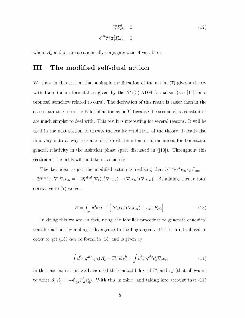
III The modified self-dual action

We show in this section that a simple modification of the action (7) gives a theory

with Hamiltonian formulation given by the SO(3)-ADM formalism (see [14] for a

proposal somehow related to ours). The derivation of this result is easier than in the

case of starting from the Palatini action as in [9] because the second class constraints

are much simpler to deal with. This result is interesting for several reasons. It will be

used in the next section to discuss the reality conditions of the theory. It leads also

in a very natural way to some of the real Hamiltonian formulations for Lorentzian

general relativity in the Ashtekar phase space discussed in ([10]). Throughout this

section all the fields will be taken as complex.

The key idea to get the modified action is realizing that ηabcdǫijkeaiebjFcdk =

−2ηabcdeai∇b∇cedi = −2ηabcd [∇b(eia∇cedi) + (∇aebi)(∇cedi)]. By adding, then, a total

derivative to (7) we get

S =∫

Md4x ηabcd

[

(∇aebi)(∇cedi) + vaeibFcdi

]

(13)

In doing this we are, in fact, using the familiar procedure to generate canonical

transformations by adding a divergence to the Lagrangian. The term introduced in

order to get (13) can be found in [15] and is given by

∫

d3x ηabcǫijk(Aia − Γi

a)ejbe

kc =

∫

d3x ηabceia∇beci (14)

in this last expression we have used the compatibility of Γia and ei

a (that allows us

to write ∂[aeib] = −ǫi

jkΓj[ae

kb]). With this in mind, and taking into account that (14)

8

generates the canonical transformations from SO(3)-ADM to the Ashtekar formalism

we expect that the action (13) leads to SO(3)-ADM (as it turns out to be the case).

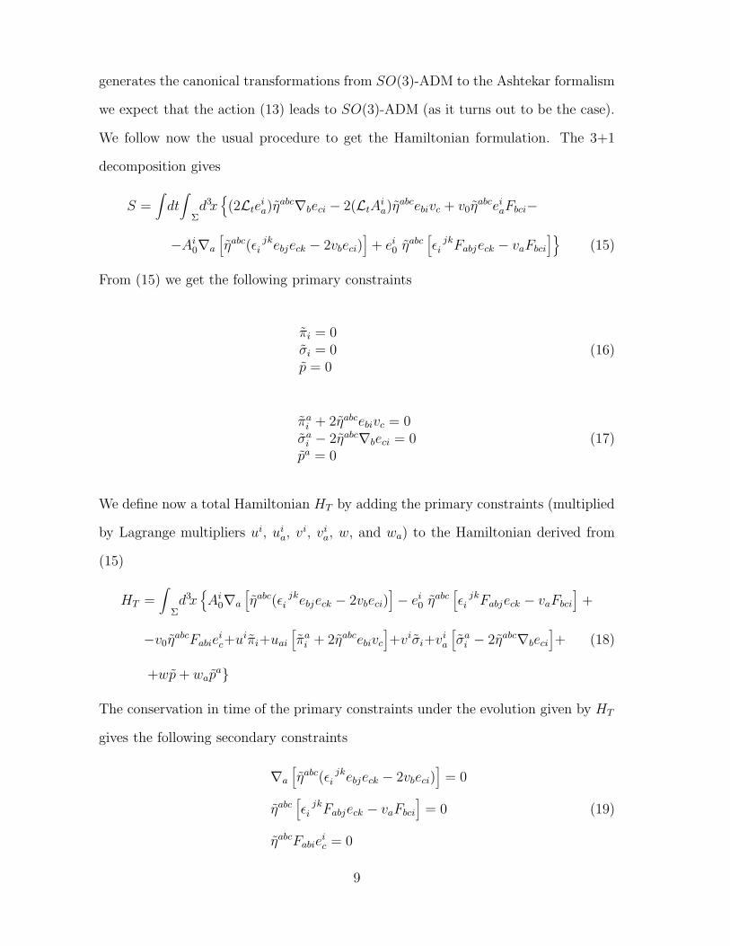
We follow now the usual procedure to get the Hamiltonian formulation. The 3+1

decomposition gives

S =∫

dt∫

Σd3x

(2Lteia)η

abc∇beci − 2(LtAia)η

abcebivc + v0ηabcei

aFbci−

−Ai0∇a

[

ηabc(ǫ jki ebjeck − 2vbeci)

]

+ ei0 ηabc

[

ǫ jki Fabjeck − vaFbci

]

(15)

From (15) we get the following primary constraints

πi = 0σi = 0p = 0

(16)

πai + 2ηabcebivc = 0

σai − 2ηabc∇beci = 0

pa = 0(17)

We define now a total Hamiltonian HT by adding the primary constraints (multiplied

by Lagrange multipliers ui, uia, vi, vi

a, w, and wa) to the Hamiltonian derived from

(15)

HT =∫

Σd3x

Ai0∇a

[

ηabc(ǫ jki ebjeck − 2vbeci)

]

− ei0 ηabc

[

ǫ jki Fabjeck − vaFbci

]

+

−v0ηabcFabie

ic+uiπi+uai

[

πai + 2ηabcebivc

]

+viσi+via

[

σai − 2ηabc∇beci

]

+ (18)

+wp + wapa

The conservation in time of the primary constraints under the evolution given by HT

gives the following secondary constraints

∇a

[

ηabc(ǫ jki ebjeck − 2vbeci)

]

= 0

ηabc[

ǫ jki Fabjeck − vaFbci

]

= 0 (19)

ηabcFabieic = 0

9

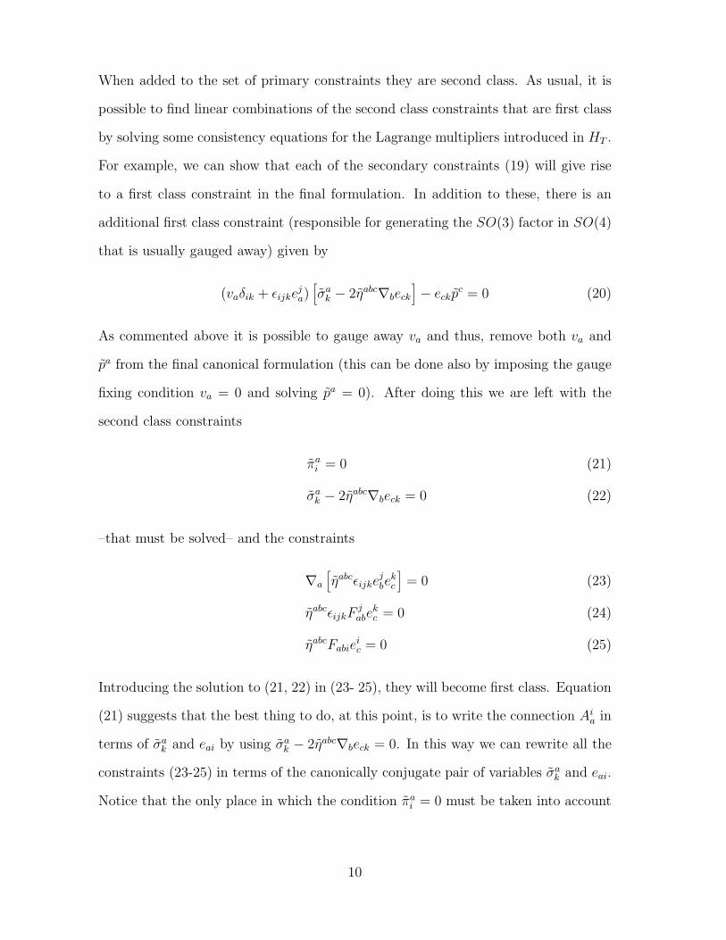
When added to the set of primary constraints they are second class. As usual, it is

possible to find linear combinations of the second class constraints that are first class

by solving some consistency equations for the Lagrange multipliers introduced in HT .

For example, we can show that each of the secondary constraints (19) will give rise

to a first class constraint in the final formulation. In addition to these, there is an

additional first class constraint (responsible for generating the SO(3) factor in SO(4)

that is usually gauged away) given by

(vaδik + ǫijkeja)

[

σak − 2ηabc∇beck

]

− eckpc = 0 (20)

As commented above it is possible to gauge away va and thus, remove both va and

pa from the final canonical formulation (this can be done also by imposing the gauge

fixing condition va = 0 and solving pa = 0). After doing this we are left with the

second class constraints

πai = 0 (21)

σak − 2ηabc∇beck = 0 (22)

–that must be solved– and the constraints

∇a

[

ηabcǫijkejbe

kc

]

= 0 (23)

ηabcǫijkFjabe

kc = 0 (24)

ηabcFabieic = 0 (25)

Introducing the solution to (21, 22) in (23- 25), they will become first class. Equation

(21) suggests that the best thing to do, at this point, is to write the connection Aia in

terms of σak and eai by using σa

k − 2ηabc∇beck = 0. In this way we can rewrite all the

constraints (23-25) in terms of the canonically conjugate pair of variables σak and eai.

Notice that the only place in which the condition πai = 0 must be taken into account

10

is in the symplectic structure5

Ω =∫

Σd3x

[

dlπai (x) ∧ dlAi

a(x) + dlσai (x) ∧ dlei

a(x)]

(26)

where it cancels the first term. This means that σak and eai are indeed a canonical

pair of variables in the final phase space. The solution to σak − 2ηabc∇beck = 0 is

Aia = Γi

a + Kia (27)

where Γia and Ki

a are given by

Γia = − 1

2e(ei

aejb − 2ej

aeib)η

bcd∂cedj (28)

Kia =

1

4e(ei

aejb − 2ej

aeib)σ

bj (29)

(e ≡ 16ηabcǫijke

iae

jbe

kc is the determinant of the triad). It is straightforward to show that

the previous Γia is compatible with ei

a (i.e. Daeib ≡ ∂ae

ib − Γc

abeic + ǫi

jkΓjae

kb = 0 where

Γcab are the Christoffel symbols built with the three dimensional metric qab ≡ ei

aebi).

Equation in (23) gives immediately (just substituting 2ηabc∇beck = σak)

ǫijkejaσ

ak = 0 (30)

This is the generator of SO(3) rotations. Differentiating now in equation (22) we get

∇aσai = 2ηabc∇a∇beci = ηabcǫijkF

jabe

kc = 0 where we have made use of (24). In order to

eliminate the Aia from ∇aσ

ai we add and subtract ǫ jk

i Γaj σak to get Daσ

ai = −ǫ jk

i Kjaσ

ak .

It is straightforward to show that the right hand side of this last expression is zero

by using the definition of Kia and the “Gauss law” (30). We have then

Daσai = 0 (31)

5dl represents the generalized exterior differential in the infinite-dimensional phase space spannedby Ai

a(x), ei

a(x), πa

i(x), and σa

i(x).

11

Finally, the scalar constraint is obtained by introducing F iab = Ri

ab + 2D[aKib] +

ǫijkK

jaK

kb (where Ri

ab ≡ 2∂[aΓib] + ǫi

jkΓjaΓ

kb is the curvature of Γi

a) in (25) and us-

ing the Gauss law (30). The final result is

ηabcRiabeci +

1

8e

[

eiae

jb − 2ej

aeib

]

σai σ

bj = 0 (32)

In order to connect this to the usual ADM and SO(3)-ADM formalisms we first

writeqab = ei

aebi

Kab =1

4e

[

2qc(aeib)σ

ci − qabe

icσ

ci

] (33)

Taking into account that pab =√

˜q(Kab−K qab) ( ˜q is the determinant of the 3-metric

qab ≡ eiaebi) we find that (33) implies6

pab =1

2e(ai σb)i (34)

These expressions allow us to immediately check that qab and pab are a pair of canon-

ically conjugate variables. By using the “Gauss law” (30) we can remove the sym-

metrizations in (34) and write pab = 12eb

i σai. With this last expression it is straight-

forward to show that the constraint (31) gives Dapab = 0 (i.e. the familiar vector

constraint in the ADM formalism). Because there is no internal symmetry in the

usual ADM formalism the only thing we are left to compute is the scalar constraint.

From (32) and using the fact that R = −ǫijkRabieaje

bk = −1

eηabcRi

abeci and σai = 2pabebi

–modulo (30)– we get

−√

˜qR +1

√

˜q

(

1

2p2 − pabpab

)

= 0 (35)

The relative signs between the potential and kinetic terms in the previous expression

correspond to Euclidean signature if we take real fields.

6ea

iis the inverse of eai.

12

In order to see how our result gives the SO(3)-ADM formalism of ref. [9] we write7

πai =

µ

2ηabcǫijke

jbe

kc (36)

Kia =

1

2µe

(

eiae

jb − 2ej

aeib

)

σbj (37)

and their inverses

eai =1

2√

µ˜π ˜ηabcǫ

ijkπbj π

ck (38)

σai = 2

√

µ˜ππ

[ai π

c]k Kk

c (39)

It is straightforward to check that these equations define a canonical transformation

for every value of the arbitrary constant µ; the relevant Poisson bracket is

πai (x), Kj

b (y)

= δab δ

ji δ

3(x, y) (40)

In the following I will use the inverse ofπa

i

˜πthat I will denote Ei

a. Substituting (38,

39) in the constraints (30-31) we easily get the “Gauss law” and the vector constraint

ǫijkKjaπ

ak = 0

Da

[

πakK

kb − δa

b πckK

kc

]

= 0 (41)

In order to get the Hamiltonian constraint we need

ηabcRiab(e)eci =

1

2√

µ˜πηabcRi

ab(e)˜ηcdeǫ

jki πd

j πfk =

1õ

Riab(E)ηabcEci = −

√

√

√

√

˜q

µR (42)

where ˜qab

= πai π

bi and we have used the fact that Riab(e) = Ri

ab(E). We also need

1

8e

[

eiae

jb − 2ej

aeib

]

σai σ

bj =

µ3/2

4˜π

[

(πai K

ia)

2 − (πai K

ja)(π

bjK

ib)

]

(43)

7 ˜π ≡ det πa

i.

13

to finally get the following Hamiltonian constraint

√

˜qR +µ2

2√

˜qπ

[bi π

a]j Ki

aKjb = 0 (44)

By choosing µ = 2 we find the result of [9].

The action introduced in this section has some nice characteristics. It shows, for

example, that it is possible to get an action for the “geometrodynamical” Husain-

Kuchar model simply by removing the term with va. It can also be used to discuss

the issue of reality conditions and to get one of the real Ashtekar formulations for

Lorentzian gravity presented in [10]. This will be the scope of the next two sections.

IV Reality conditions

In this section I will show how the action (13) can be used to discuss the reality

conditions of the theory and the signature of the space-time. The starting point

is realizing that since we are working with complex fields, multiplying (13) by a

purely imaginary factor (say i) cannot have any effect on the theory (because the

field equations will remain unchanged). However, same produces some changes in the

Hamiltonian formulation. Following the derivation presented in the previous section

we find now that the primary constraints are

πi = 0σi = 0p = 0

(45)

πai + 2iηabcebivc = 0

σai − 2iηabc∇beci = 0

pa = 0(46)

14

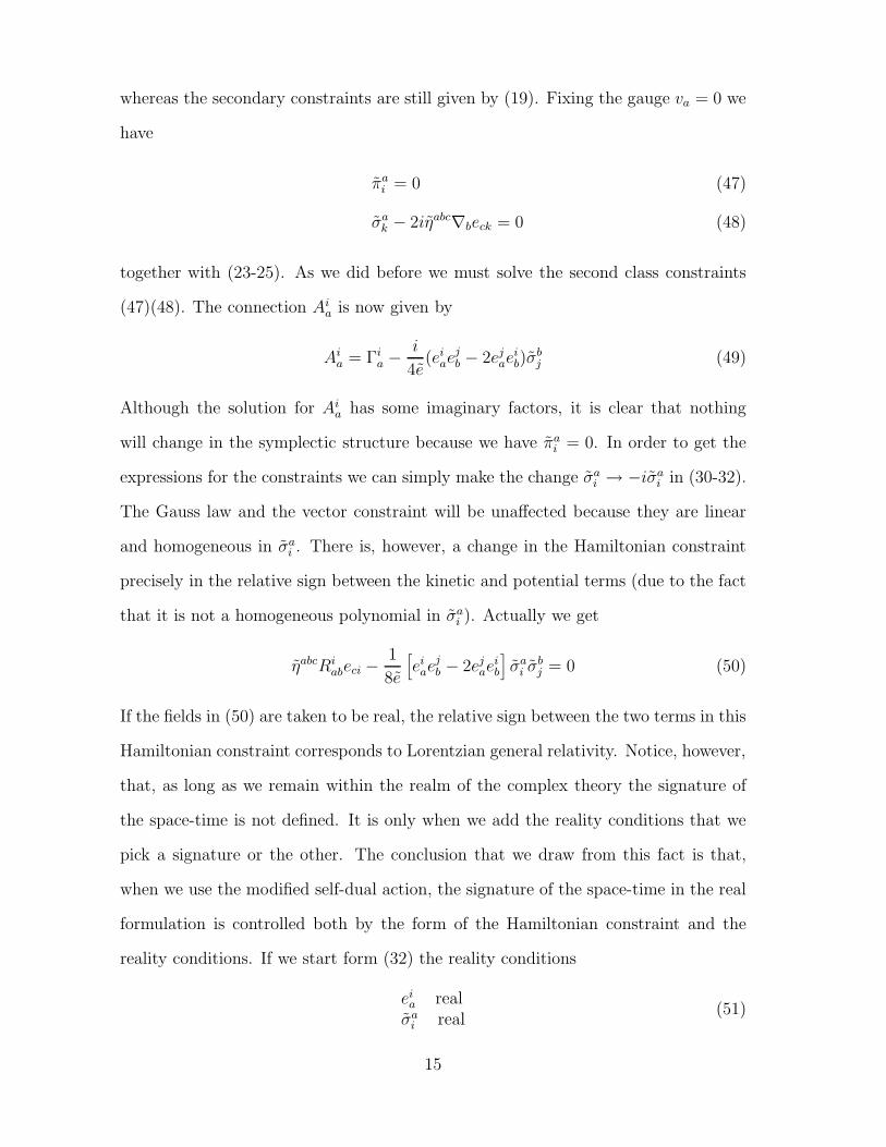
whereas the secondary constraints are still given by (19). Fixing the gauge va = 0 we

have

πai = 0 (47)

σak − 2iηabc∇beck = 0 (48)

together with (23-25). As we did before we must solve the second class constraints

(47)(48). The connection Aia is now given by

Aia = Γi

a −i

4e(ei

aejb − 2ej

aeib)σ

bj (49)

Although the solution for Aia has some imaginary factors, it is clear that nothing

will change in the symplectic structure because we have πai = 0. In order to get the

expressions for the constraints we can simply make the change σai → −iσa

i in (30-32).

The Gauss law and the vector constraint will be unaffected because they are linear

and homogeneous in σai . There is, however, a change in the Hamiltonian constraint

precisely in the relative sign between the kinetic and potential terms (due to the fact

that it is not a homogeneous polynomial in σai ). Actually we get

ηabcRiabeci −

1

8e

[

eiae

jb − 2ej

aeib

]

σai σ

bj = 0 (50)

If the fields in (50) are taken to be real, the relative sign between the two terms in this

Hamiltonian constraint corresponds to Lorentzian general relativity. Notice, however,

that, as long as we remain within the realm of the complex theory the signature of

the space-time is not defined. It is only when we add the reality conditions that we

pick a signature or the other. The conclusion that we draw from this fact is that,

when we use the modified self-dual action, the signature of the space-time in the real

formulation is controlled both by the form of the Hamiltonian constraint and the

reality conditions. If we start form (32) the reality conditions

eia real

σai real

(51)

15

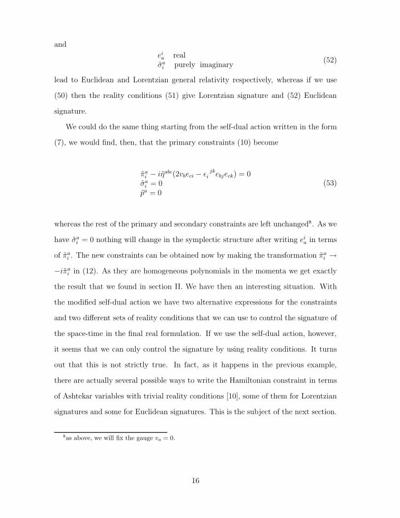
and

eia real

σai purely imaginary

(52)

lead to Euclidean and Lorentzian general relativity respectively, whereas if we use

(50) then the reality conditions (51) give Lorentzian signature and (52) Euclidean

signature.

We could do the same thing starting from the self-dual action written in the form

(7), we would find, then, that the primary constraints (10) become

πai − iηabc(2vbeci − ǫ jk

i ebjeck) = 0σa

i = 0pa = 0

(53)

whereas the rest of the primary and secondary constraints are left unchanged8. As we

have σai = 0 nothing will change in the symplectic structure after writing ei

a in terms

of πai . The new constraints can be obtained now by making the transformation πa

i →

−iπai in (12). As they are homogeneous polynomials in the momenta we get exactly

the result that we found in section II. We have then an interesting situation. With

the modified self-dual action we have two alternative expressions for the constraints

and two different sets of reality conditions that we can use to control the signature of

the space-time in the final real formulation. If we use the self-dual action, however,

it seems that we can only control the signature by using reality conditions. It turns

out that this is not strictly true. In fact, as it happens in the previous example,

there are actually several possible ways to write the Hamiltonian constraint in terms

of Ashtekar variables with trivial reality conditions [10], some of them for Lorentzian

signatures and some for Euclidean signatures. This is the subject of the next section.

8as above, we will fix the gauge va = 0.

16

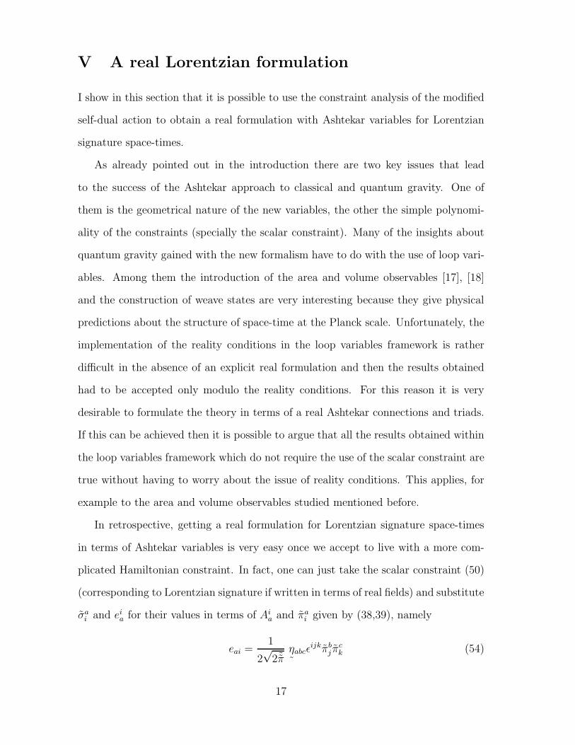
V A real Lorentzian formulation

I show in this section that it is possible to use the constraint analysis of the modified

self-dual action to obtain a real formulation with Ashtekar variables for Lorentzian

signature space-times.

As already pointed out in the introduction there are two key issues that lead

to the success of the Ashtekar approach to classical and quantum gravity. One of

them is the geometrical nature of the new variables, the other the simple polynomi-

ality of the constraints (specially the scalar constraint). Many of the insights about

quantum gravity gained with the new formalism have to do with the use of loop vari-

ables. Among them the introduction of the area and volume observables [17], [18]

and the construction of weave states are very interesting because they give physical

predictions about the structure of space-time at the Planck scale. Unfortunately, the

implementation of the reality conditions in the loop variables framework is rather

difficult in the absence of an explicit real formulation and then the results obtained

had to be accepted only modulo the reality conditions. For this reason it is very

desirable to formulate the theory in terms of a real Ashtekar connections and triads.

If this can be achieved then it is possible to argue that all the results obtained within

the loop variables framework which do not require the use of the scalar constraint are

true without having to worry about the issue of reality conditions. This applies, for

example to the area and volume observables studied mentioned before.

In retrospective, getting a real formulation for Lorentzian signature space-times

in terms of Ashtekar variables is very easy once we accept to live with a more com-

plicated Hamiltonian constraint. In fact, one can just take the scalar constraint (50)

(corresponding to Lorentzian signature if written in terms of real fields) and substitute

σai and ei

a for their values in terms of Aia and πa

i given by (38,39), namely

eai =1

2√

2˜π ˜ηabcǫ

ijkπbj π

ck (54)

17

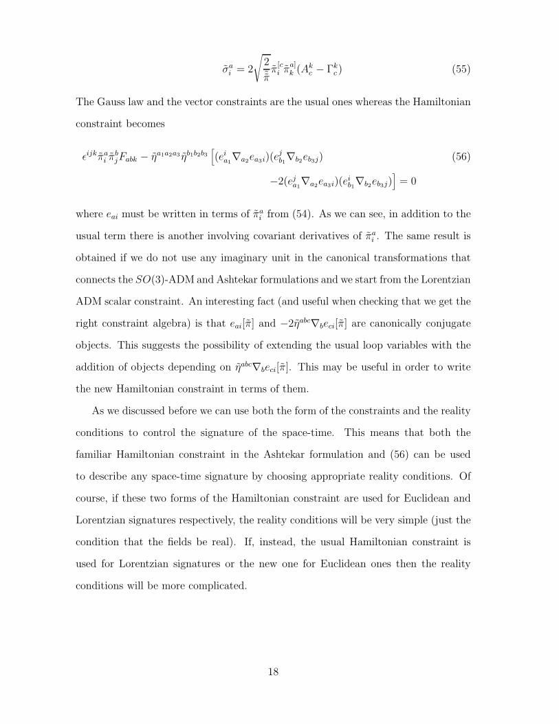
σai = 2

√

2˜ππ

[ci π

a]k (Ak

c − Γkc ) (55)

The Gauss law and the vector constraints are the usual ones whereas the Hamiltonian

constraint becomes

ǫijkπai π

bjFabk − ηa1a2a3 ηb1b2b3

[

(eia1∇a2

ea3i)(ejb1∇b2eb3j) (56)

−2(eja1∇a2

ea3i)(eib1∇b2eb3j)

]

= 0

where eai must be written in terms of πai from (54). As we can see, in addition to the

usual term there is another involving covariant derivatives of πai . The same result is

obtained if we do not use any imaginary unit in the canonical transformations that

connects the SO(3)-ADM and Ashtekar formulations and we start from the Lorentzian

ADM scalar constraint. An interesting fact (and useful when checking that we get the

right constraint algebra) is that eai[π] and −2ηabc∇beci[π] are canonically conjugate

objects. This suggests the possibility of extending the usual loop variables with the

addition of objects depending on ηabc∇beci[π]. This may be useful in order to write

the new Hamiltonian constraint in terms of them.

As we discussed before we can use both the form of the constraints and the reality

conditions to control the signature of the space-time. This means that both the

familiar Hamiltonian constraint in the Ashtekar formulation and (56) can be used

to describe any space-time signature by choosing appropriate reality conditions. Of

course, if these two forms of the Hamiltonian constraint are used for Euclidean and

Lorentzian signatures respectively, the reality conditions will be very simple (just the

condition that the fields be real). If, instead, the usual Hamiltonian constraint is

used for Lorentzian signatures or the new one for Euclidean ones then the reality

conditions will be more complicated.

18

VI Conclusions and outlook

By using a modified form of the self-dual action that leads to the SO(3)-ADM formal-

ism without the appearance of difficult second class constraints we have studied the

reality conditions of the theory and obtained a real formulation in terms of Ashtekar

variables for Lorentzian signature space-times. We have been able to show that,

both in the ADM and Ashtekar phase spaces, it is possible to find different forms for

the Hamiltonian constraints for complexified general relativity. In order to pass to

a real formulation we need to impose reality conditions that can be chosen to pick

the desired space-time signature. In a sense, it is no longer necessary to talk about

reality conditions because we can impose the trivial ones (real fields) and control the

signature of the space time by choosing appropriate Hamiltonian constraints.

The fact that a real formulation in the Ashtekar phase space is available means that

all the results obtained by using loop variables that are independent of the detailed

form of the Hamiltonian constraint are true without having to worry about reality

conditions. On the other hand there a price to be paid; namely, that the Hamiltonian

constraint is no longer a simple quadratic expression in both the densitized triad and

the Ashtekar connection. This makes it more difficult to discuss all those issues that

depend critically on having the theory formulated in terms of simple constraints; in

particular solving the constraints will be more difficult now.

In this respect one can honestly say that the structure of the Hamiltonian con-

straint presented above (or the alternative forms discussed in [10]) is, at least, as

complicated as the one of the familiar ADM constraint. In spite of that, some inter-

esting and basic features of the Ashtekar formulation are retained. The phase space

still corresponds to that of a Yang-Mills theory, so we can continue to use loop vari-

ables in the passage to the quantum theory. The “problem” of reality conditions has

now been transformed into that of writing the new (and complicated) Hamiltonian

constraint in terms of loop variables and solving the quantum version of the con-

19

straints acting on the wave functional. The final success of this approach will depend

on the possibility of achieving this goal.

One interesting point of discussion suggested by the results presented in the paper

has to do with the obvious asymmetry between the formulations of gravity in a real

Ashtekar phase space for Lorentzian and Euclidean signatures. In the geometrody-

namical approach, there is little difference, both in the Lagrangian and Hamiltonian

formulations, between them (at least at the superficial level of the complication of the

expressions involved). In fact it all boils down to the relative signs between the poten-

tial and kinetic terms in the scalar constraint. In our case, however, the formulations

that we get are, indeed, rather different.

The existence of the formulation presented in this paper also suggests that the

origin of the signature at the Lagrangian level is also rather obscure. From the (real)

self-dual-action it seems quite natural to associate, for example, the euclidean signa-

ture with the fact that the gauge group is SO(4) and the metric is eaIeIb . However,

the observation that one of the SO(3) factors “disappears” from the theory may be

telling us that, perhaps, it is not necessary to start with an SO(4) internal symmetry.

In fact the Capovilla-Dell-Jacobson [19] Lagrangian leads to the same formulation

using only SO(3) as the internal symmetry.

Although we still do not have a four dimensional Lagrangian formulation of the

theory, the marked asymmetry between the real Hamiltonian formulations for dif-

ferent space-time signature strongly suggests that it would differ very much from

the usual self-dual action (a fact also supported by the lack of success of all the at-

tempts to get Lorentzian general relativity by introducing simple modifications in the

known actions). This could have intriguing consequences in a perturbative setting

because the UV behavior (controlled to a great extent by the functional form of the

Lagrangian) of the Euclidean and the Lorentzian theories could be very different. It

is worthwhile to remember at this point that the Einstein-Hilbert action and the so

20

called higher derivative theories, that differ in some terms quadratic in the curvatures,

have very different UV behaviors. The first one is non-renormalizable whereas the

second one is renormalizable but non-unitary. In our opinion this is an issue that

deserves further investigation.

Acknowledgements I wish to thank A. Ashtekar, Ingemar Bengtsson, Peter

Peldan, Lee Smolin and Chopin Soo for several interesting discussions and remarks.

I am also grateful to the Consejo Superior de Investigaciones Cientıficas (Spanish

Research Council )for providing financial support.

References

[1] A. Ashtekar, Phys. Rev. Lett. 57, 2244 (1986)

A. Ashtekar, Phys. Rev. D36, 1587 (1987)

A. Ashtekar Non Perturbative Canonical Gravity (Notes prepared in collabora-

tion with R. S. Tate) (World Scientific Books, Singapore, 1991)

[2] Bibliography of publications related to Classical and Quantum Gravity in terms

of the Ashtekar Variables, updated by T. Schilling gr-qc 9409031

[3] C. Rovelli and L. Smolin, Phys. Rev. Lett. 61, 1155 (1988)

C. Rovelli and L. Smolin, Nucl. Phys. B331, 80 (1990)

[4] R. Arnowitt, S. Deser, and C. W. Misner The Dynamics of General Relativity

in Gravitation, an introduction to current research edited by L. Witten (Wiley

1962)

[5] A. Ashtekar, J. Lewandowski, D. Marolf, J. Mourao, T. Thiemann, in prepara-

tion.

[6] J. F. Barbero G. Int. J. Mod. Phys. D3, 397 (1994)

J. F. Barbero G. Phys. Rev. D49, 6935 (1994)

21

[7] J. Samuel Pramana J. Phys. 28, L429 (1987)

T. Jacobson and L. Smolin Phys. Lett. B196, 39 (1987)

T. Jacobson and L. Smolin Class. Quantum Grav. 5, 583 (1988)

[8] V. Husain and K. Kuchar Phys. Rev. D42, 4070 (1990)

[9] A. Ashtekar, A. P. Balachandran and S. G. Jo Int. J. Mod. Phys A4, 1493 (1989)

[10] J. F. Barbero G. Real Ashtekar Variables for Lorentzian Signature Space-times

Preprint CGPG-PSU, gr-qc

[11] Chopin Soo, private communication.

[12] M. Henneaux, J. E. Nelson and C. Schomblond Phys. Rev. D39, 434 (1989)

[13] Dirac P.A.M. in Lectures on Quantum Mechanics, Belfer Graduate School of

Science Monograph Series Number Two, Yeshiva University, New York, (1964)

[14] R. P. Wallner Phys. Rev. D46, 4263 (1992)

[15] B. P. Dolan Phys. Lett. B233, 89 (1989)

[16] J. F. Barbero G. in preparation

[17] C. Rovelli and L. Smolin Quantization of Area and Volume Pittsburgh and

CGPG-PSU preprint

[18] A. Ashtekar, C. Rovelli and L. Smolin Phys. REv. Lett. 69, 237 (1992)

[19] R. Capovilla, J. Dell, and T. Jacobson Phys. Rev. Lett. 63, 2325 (1989)

22