Dr. J. Bikker Realistic Image Synthesis 1 lecture Realistic Image Synthesis

Welcome message from author
This document is posted to help you gain knowledge. Please leave a comment to let me know what you think about it! Share it to your friends and learn new things together.
Transcript
Dr. J. Bikker
Realistic Image Synthesis
1lecture
Realistic Image Synthesis
Today:
Introduction
Virtual World Representations
Rendering Algorithm Overview
Light Transport
History of Realistic Rendering
Further Reading

Realistic Image Synthesis:
An exploration of light transport and rendering theory and technology.

Realistic Image Synthesis:
An exploration of physically based techniques.

Course Setup
IS is a conceptual course within the Master Game Technology.The IS course consists of 6 lectures.Large amount of papers available from my GoogleDrive:
https://drive.google.com/folderview?id=0B-Bsn1Q3OY4GNm5nUGZQYi1sVVE&usp=sharing

Course Setup
28/1 Lecture 1: Introduction, virtual world representations, rendering fundamentals4/2 Lecture 2: Ray tracing: Whitted, Cook, Kajiya11/2 Lecture 3: Student presentations on theme “physically based”18/2 holiday25/2 Lecture 4: Physically based materials: BRDFs4/3 Lecture 5: Path tracing details: probabilities11/3 no lecture18/3 no lecture25/3 Lecture 6 (SW): To be determined.
All topics tentative.

Today:
Introduction
Virtual World Representations
Rendering Algorithm Overview
Light Transport
History of Realistic Rendering
Further Reading
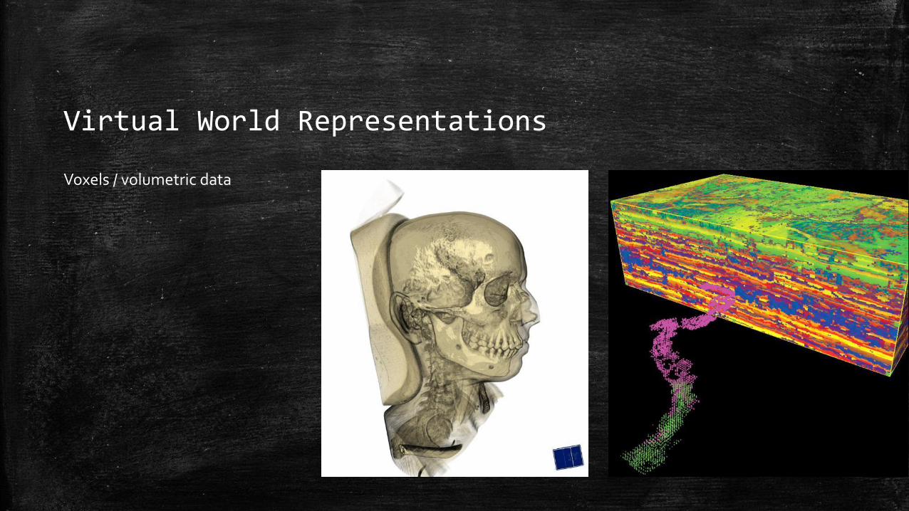
Virtual World Representations
Voxels / volumetric data

Virtual World Representations
Polygons
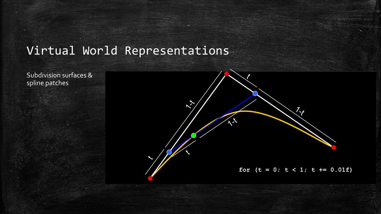
Virtual World Representations
Subdivision surfaces & spline patches
for (t = 0; t < 1; t += 0.01f)

Virtual World Representations
Subdivision surfaces & spline patches
http://design.osu.edu/carlson/history/PDFs/meet-geri.pdf

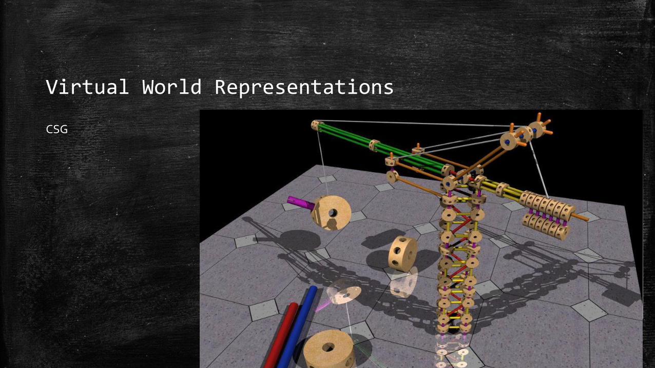
Virtual World Representations
CSG

Virtual World Representations
Implicit surfaces
Example: D(r) = 1 / r2
(from:http://paulbourke.net/geometry/implicitsurf )
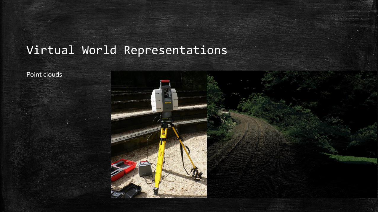
Virtual World Representations
Point clouds

Virtual World Representations
Digest:
World representation depends on acquisition technology / modeling preferences.
In games, we are accustomed to adapting data to the rendering algorithm.
In movies, this is typically not the case; modeling and animation take precedence.
In various other fields (e.g. medical visualization, architecture) scanning technology
dictates the representation.

Today:
Introduction
Virtual World Representations
Rendering Algorithm Overview
Light Transport
History of Realistic Rendering
Further Reading

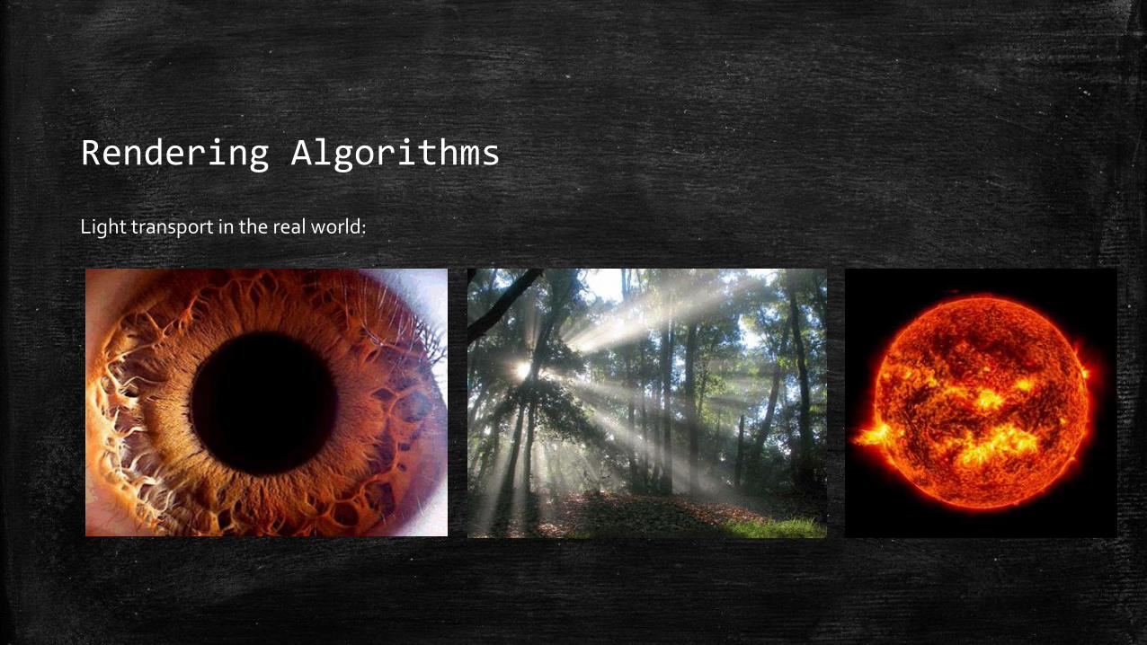
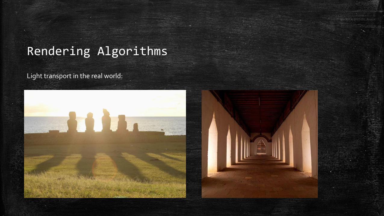
Rendering Algorithms
Light transport in the real world:

Rendering Algorithms
Light transport in the real world:

Rendering Algorithms
Light transport in the real world:
Rendering Algorithms
Light transport in the real world:

Rendering Algorithms
Light transport in the real world:
1. Light emission
2. Interactions: reflection, refraction, absorption (… ,dispersion)
3. Detection
Important: objects can be perceived because they either emit or reflect light.

Rendering Algorithms
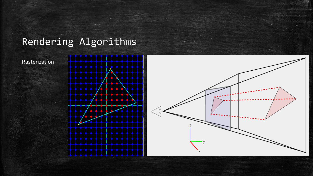
Rasterization
Rendering Algorithms
Rasterization

Rendering Algorithms
Rasterization
"Objects can be perceived because they either emit or reflect light."
Modern rasterization:
Renders triangles one by one Triangles can have a material (texture,
normal map) Triangles can be lit
√ Reflection of direct light
√ Occlusion (shadows), using stencil buffer, point lights only
X Reflection of environment
X Reflection of indirect light

Rendering Algorithms
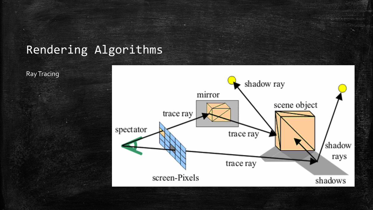
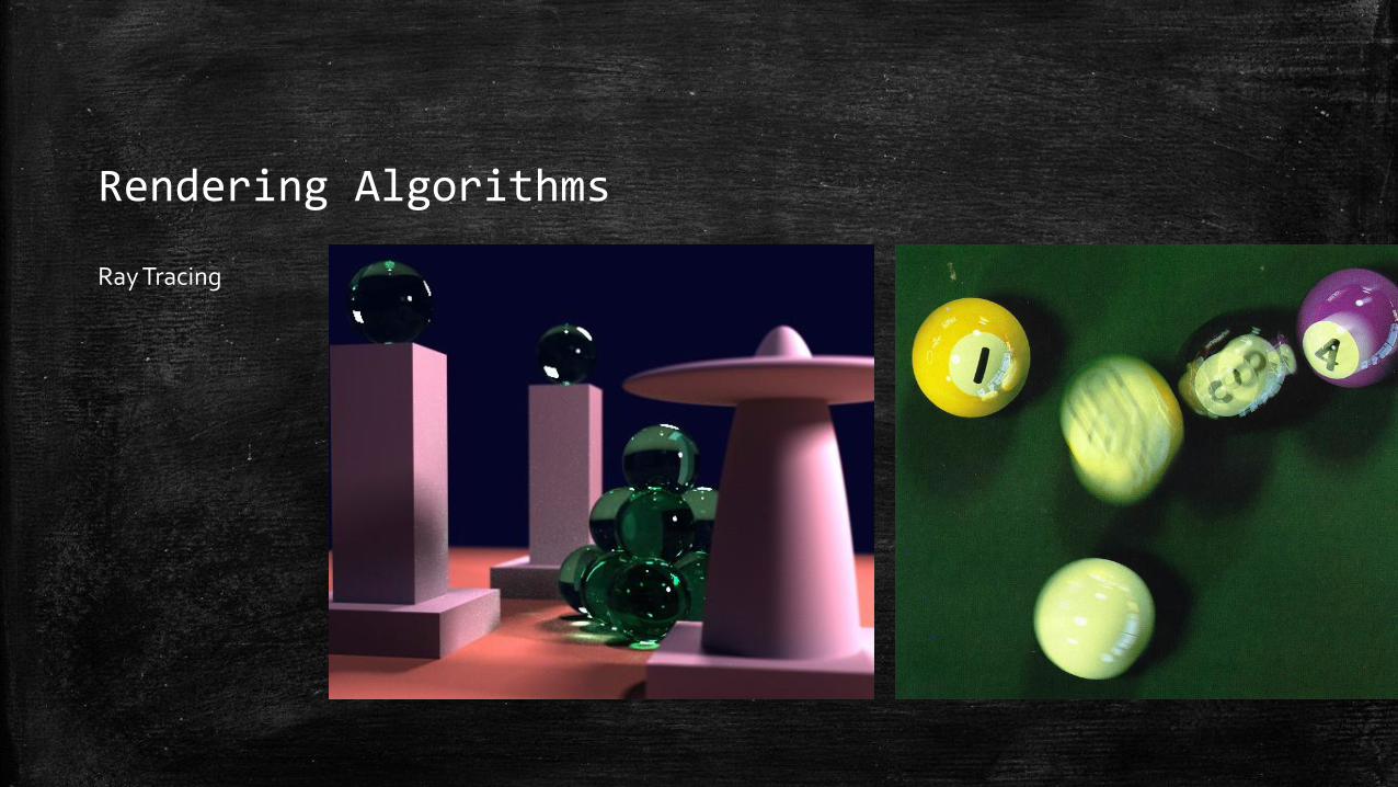
Ray Tracing
Rendering Algorithms
Ray Tracing

Rendering Algorithms
Ray Tracing
"Objects can be perceived because they either emit or reflect light."
Ray Tracing:
Finds intersection of rays through pixels with scene geometry Rays ‘bounce off’ of reflective materials Completes light transport paths using shadow rays
√ Reflection of direct and indirect light
√ Occlusion (shadows) for indirect and direct light
√ Reflection of environment
√ Reflection of indirect light

Today:
Introduction
Virtual World Representations
Rendering Algorithm Overview
Light Transport
History of Realistic Rendering
Further Reading

Light Transport Fundamentals
Rendering Equation:
Light from x to eye equals:
1. Light emitted from x towards eye;2. Light reflected by x
Note:
x reflects light arriving from all directions Ω
Reflected light is scaled by BRDF
Reflected light is scaled by –w · n
The equation is recursive

Light Transport Fundamentals
Rendering Equation
Light from x to eye equals:
1. Light emitted from x towards eye;2. Light reflected by x
Note:
x reflects light arriving from all directions Ω
Reflected light is scaled by BRDF
Reflected light is scaled by –w · n
nw'
n
w'

Light Transport Fundamentals
Rendering Equation
Light from x to eye equals:
1. Light emitted from x towards eye;2. Light reflected by x
Note:
x reflects light arriving from all directions Ω
Reflected light is scaled by BRDF
Reflected light is scaled by –w · n
n
w'

Light Transport Fundamentals
Rendering Equation
Light from x to eye equals:
1. Light emitted from x towards eye;2. Light reflected by x
Note:
x reflects light arriving from all directions Ω
Reflected light is scaled by BRDF
Reflected light is scaled by –w · n
nw'w

Light Transport Fundamentals
Rendering Equation
Light from x to eye equals:
1. Light emitted from x towards eye;2. Light reflected by x
Note:
x reflects light arriving from all directions Ω
Reflected light is scaled by BRDF
Reflected light is scaled by –w · n
nw'w

Light Transport Fundamentals
Particle model:
Out of 1 million particles arriving at x from alldirections, how many end up in our eye?
Proportional to –w · n Proportional to BRDF
n
w'
nw'w
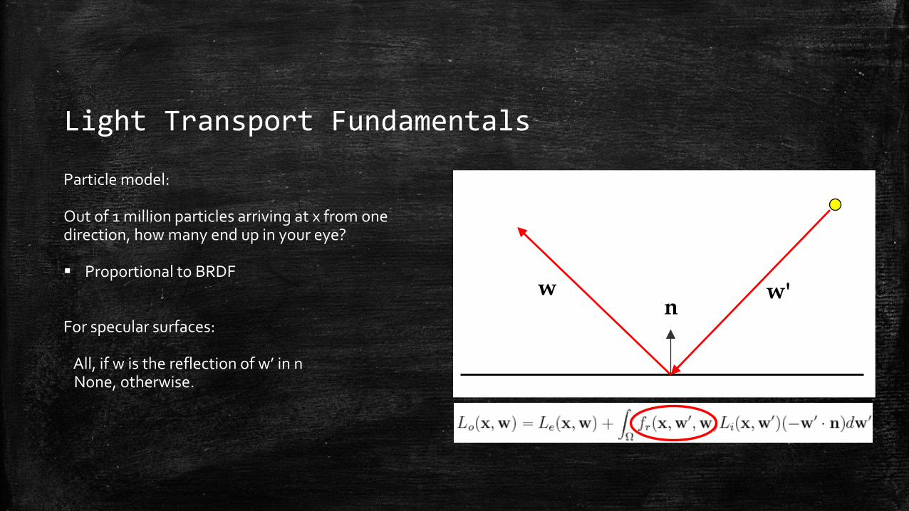
Light Transport Fundamentals
Particle model:
Out of 1 million particles arriving at x from onedirection, how many end up in your eye?
Proportional to BRDF
For specular surfaces:
All, if w is the reflection of w’ in nNone, otherwise.

nw'w
Light Transport Fundamentals
Particle model:
Out of 1 million particles arriving at x from onedirection, how many end up in your eye?
Proportional to BRDF
For diffuse surfaces:
The number is proportional to n ·w
and:the material color.
nw'w
Light Transport Fundamentals
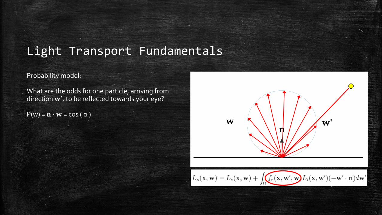
Probability model:
What are the odds for one particle, arriving fromdirection w’, to be reflected towards your eye?
P(w) = n ·w = cos ( α )

Pure particle simulation:
Yields a correct image
Some particles leave the scene
Some particles have complex paths
May take a while before every
pixel receives several particles
This process is referred to asforward ray tracing.

Backward ray tracing:
Yields a correct image
Some particles leave the scene
Some paths are complex
May take a while before every pixel has enough paths that connect to a light
(use large lights to overcomebiggest hurdle)
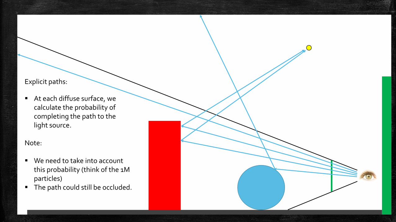
Explicit paths:
At each diffuse surface, wecalculate the probability ofcompleting the path to thelight source.
Note:
We need to take into accountthis probability (think of the 1Mparticles)
The path could still be occluded.
Light Transport Fundamentals
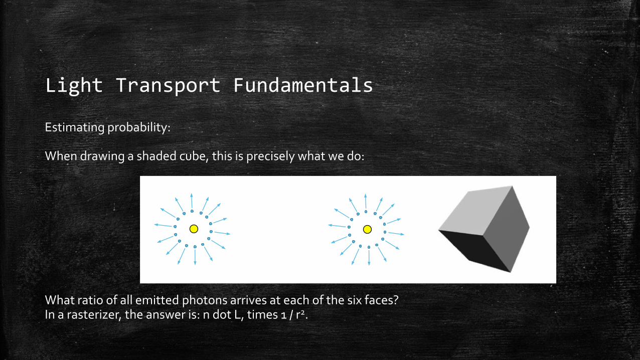
Estimating probability:
When drawing a shaded cube, this is precisely what we do:
What ratio of all emitted photons arrives at each of the six faces? In a rasterizer, the answer is: n dot L, times 1 / r2.


Light Transport Fundamentals
Digest:
Pure particle tracing can be done either forward or backward, yielding the same result, but typically different efficiency.
Rather than waiting for paths to randomly occur, we can calculate their probability instead.
The calculation of ‘direct illumination’ in any rasterizer (as well as every ray tracer) is fundamentally a probability estimation.

Today:
Introduction
Virtual World Representations
Rendering Algorithm Overview
Light Transport
History of Realistic Rendering
Further Reading
History of Realistic Rendering
Appel
A. Appel. “Some Techniques for Shading Machine Renderings of Solids”, in: AFIPS ’68 (Spring): Proceedings of the April 30–May 2, 1968 Spring Joint Computer Conference, pages 37–45.
History of Realistic Rendering
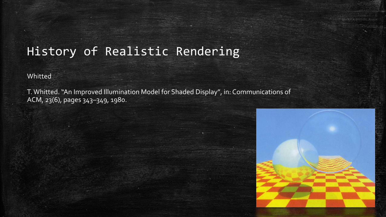
Whitted
T. Whitted. “An Improved Illumination Model for Shaded Display”, in: Communications of ACM, 23(6), pages 343–349, 1980.
History of Realistic Rendering
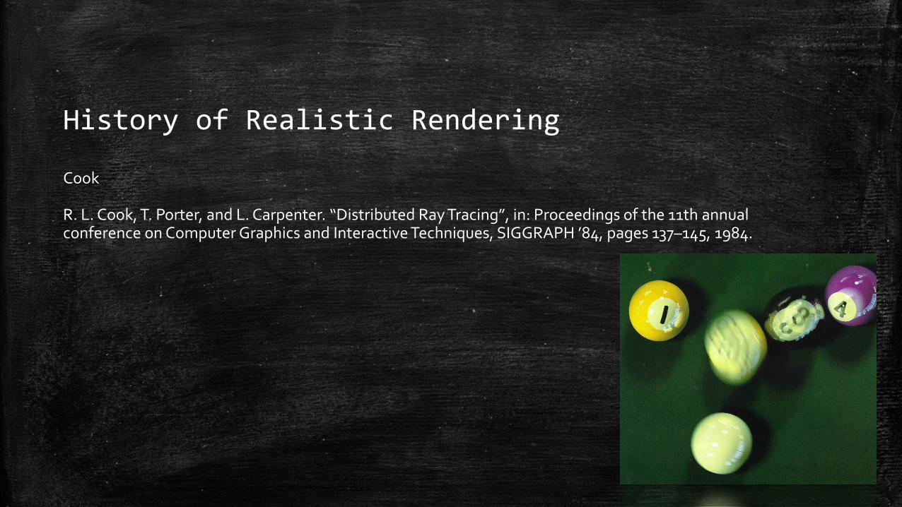
Cook
R. L. Cook, T. Porter, and L. Carpenter. “Distributed Ray Tracing”, in: Proceedings of the 11th annual conference on Computer Graphics and Interactive Techniques, SIGGRAPH ’84, pages 137–145, 1984.

History of Realistic Rendering
Kajiya
J. T. Kajiya. ”The Rendering Equation”, in: Proceedings of the 13th annual conference on Computer Graphics and Interactive Techniques, SIGGRAPH ’86, pages 143–150.

History of Realistic Rendering
Veach
E. Veach. “Robust Monte Carlo Methods for Light Transport Simulation”. Ph.D. thesis, Stanford University, 1997.
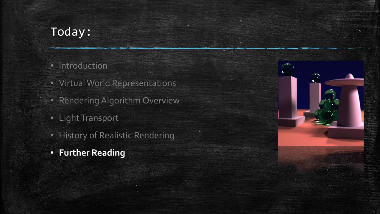
Today:
Introduction
Virtual World Representations
Rendering Algorithm Overview
Light Transport
History of Realistic Rendering
Further Reading

Further Reading
Turner Whitted: An Improved Illumination Model for Shaded Display.
Cook et al.: Distributed Ray Tracing.
James Kajiya: The Rendering Equation.
THE ENDnext week: ray tracing algorithms

Related Documents


