Realistic evolutionary Realistic evolutionary models models Marjolijn Elsinga & Lars Hemel

Welcome message from author
This document is posted to help you gain knowledge. Please leave a comment to let me know what you think about it! Share it to your friends and learn new things together.
Transcript
Realistic evolutionary modelsRealistic evolutionary models
Marjolijn Elsinga & Lars Hemel

Realistic evolutionary modelsRealistic evolutionary models
Contents• Models with different rates at different sites• Models which allow gaps• Evaluating different models• Break• Probabilistic interpretation of Parsimony• Maximum Likelihood distances

Unrealistic assumptionsUnrealistic assumptions
1 Same rate of evolution at each site in the substitution matrix
- In reality: the structure of proteins and the base pairing of RNA result in different rates
2 Ungapped alignments
- Discard useful information given by the pattern of deletions and insertions

Different rates in matrixDifferent rates in matrix
Maximum likelihood, sites are independent
Xj for j = 1…n

Different rates in matrix (2)Different rates in matrix (2)
Introduce a site-dependent variable ru

Different rates in matrix (3)Different rates in matrix (3)
We don’t know ru, so we use a prior
Yang [1993] suggests a gamma distribution g(r, α , α), with mean = 1 and variance = 1/α

ProblemProblem
Number of terms grows exponentially with the number of sequences computationally slow
Solution: approximation- Replace integral by a discrete sum- Subdivide domain into m intervals- Let rk denote the mean of the gamma
distribution in the kth interval

SolutionSolution
Yang [1993] found m = 3.4 gives a good approximation
Only m times as much computation as for non-varying sites

Evolutionary models with gaps (1)Evolutionary models with gaps (1)
Idea 1: introduce ‘_’ as an extra character of the alphabet of K residues and replace the (KxK) matrix with a (K+1) x (K+1) matrix
Drawback: no possibility to assign lower cost to a following gap, gaps are now independent
Evolutionary models with gaps (2)Evolutionary models with gaps (2)
Idea 2: Allison, Wallace & Yee [1992] introduce delete and insertion states to ensure affine-type gaps
Drawback: computationally intractable

Evolutionary models with gaps (3)Evolutionary models with gaps (3)
Idea 3: Thorne, Kishino & Felsenstein [1992] use fragment substitution to get a degree of biological plausibility
Drawback: usable for only two sequences

FinallyFinally
Find a way to use affine-type gap penalties in a computationally reasonable way
Mitchison & Durbin [1995] made a tree HMM which uses a profile HMM architecture, and treats paths through the model as objects that undergo evolutionary change

Assumptions needed againAssumptions needed again
We will use a architecture quite simpler than that of the profile HMM of Krogh et al [1994]: it has only match and delete states
Match state: Mk
Delete state: Dk k = position in the model

Tree HMM with gaps (1)Tree HMM with gaps (1)
Sequence y is ancestor of sequence xBoth sequences are aligned to the
model, so both follow a prescribed path through the model

Tree HMM with gaps (2)Tree HMM with gaps (2)
x emits residu xi at Mk
y emits residu yj at Mk
Probability of substitution yj xi is
P(xi| yj,t)

Tree HMM with gaps (3)Tree HMM with gaps (3)
What if x goes a different path than yx: Mk Dk+1 (= MD)
y: Mk Mk+1 (= MM)
P(MD|MM, t)
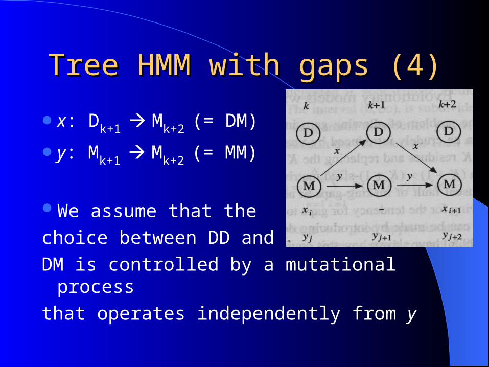
Tree HMM with gaps (4)Tree HMM with gaps (4)
x: Dk+1 Mk+2 (= DM)
y: Mk+1 Mk+2 (= MM)
We assume that the
choice between DD and
DM is controlled by a mutational process
that operates independently from y
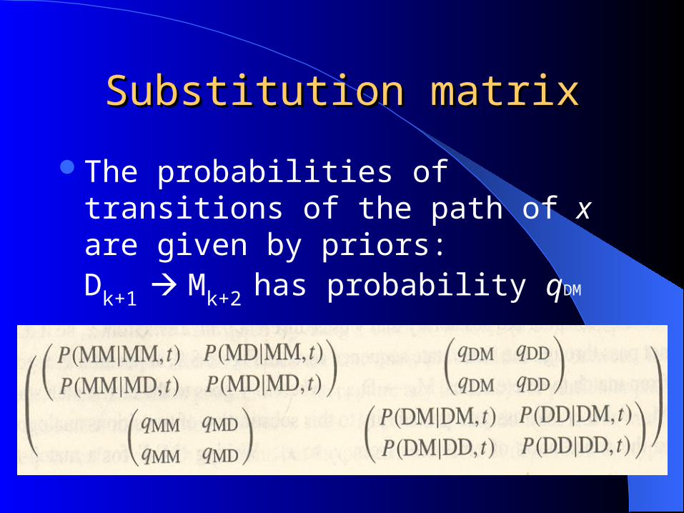
Substitution matrixSubstitution matrix
The probabilities of transitions of the path of x are given by priors: Dk+1 Mk+2 has probability qDM

How it worksHow it works
At position k: qyjP(xi|yj,t)
Transition k k+1:
qMMP(MD|MM,t)
Transition k+1 k+2:
qMMqDM

An other exampleAn other example

Evaluating models: evidenceEvaluating models: evidence
Comparing models is difficultCompare probabilities:
P(D|M1) and P(D|M2) by integrating
over all parameters of each modelParameters θ Prior probabilities P(θ )

Comparing two modelsComparing two models
Natural way to compare M1 and M2 is to
compute the posterior probability of M1

Parametric BootstrapParametric Bootstrap
Let be the maximum likelihood of the data D for the model M1
Let be the maximum likelihood of the data D for the model M2
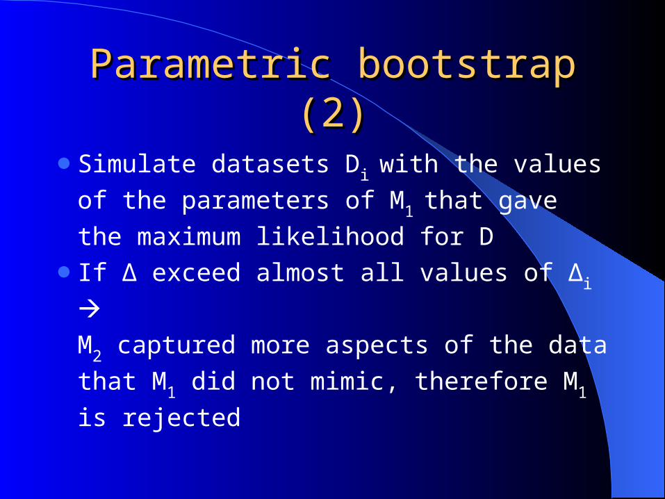
Parametric bootstrap (2)Parametric bootstrap (2)
Simulate datasets Di with the values of
the parameters of M1 that gave the
maximum likelihood for DIf Δ exceed almost all values of Δi
M2 captured more aspects of the data
that M1 did not mimic, therefore M1 is
rejected

BreakBreak

Probabilistic interpretation of Probabilistic interpretation of various modelsvarious models
Lars Hemel
OverviewOverviewReview of last week’s method Parsimony
– Assumptions, PropertiesProbabilistic interpretation of ParsimonyMaximum Likelihood distances
– Example: Neighbour joiningMore probabilistic interpretations
– Sankoff & Cedergren– Hein’s affine cost algorithm
Conclusion / Questions?
ReviewReview
Parsimony = Finding a tree which can explain the observed sequences with a minimal number of substitutions

ParsimonyParsimony
Remember the following assumptions:– Sequences are aligned– Alignments do not have gaps– Each site is treated independently
Further more, many families have:– Substitution matrix is multiplicative:– Reversibility: ba qtbaPqtabP ),|(),|(
S(t)S(s)s)S(t

ParsimonyParsimony
Basic step: counting the minimal number of changes for one site
Final number of substitutions is summing over all the sites
Weighted parsimony uses different ‘weights’ for different substitutions

Probabilistic interpretation of Probabilistic interpretation of parsimonyparsimony
Given: A set of substitution probabilities P(b|a) in which we neglect the dependence on length
t Calculate substitution costs
S(a,b) = -log P(b|a) Felsenstein [1981] showed that by using these
substitution costs, the minimal cost at site u for the whole tree T obtained by the weighted parsimony algorithm is regarded as an approximation to the likelihood

Probabilistic interpretation of Probabilistic interpretation of parsimonyparsimony
Testing performance for tree-building algorithms can be done by generating trees probabilistic with sampling and then see how often a given algorithm reconstructs them correctly
Sampling is done as follows:– Pick a residue a at the root with probability – Accept substitution to b along the edge down to node i
with probability repetitive– Sequences of length N are generated by N independent
repetitions of this procedure– Maximum likelihood should reconstruct the correct tree
for large N
aq
),|( itabP

Probabilistic interpretation of Probabilistic interpretation of parsimonyparsimony
Suppose we have tree T, with the following edgelengths
0.09
0.1
0.1
0.3
0.3T
pp
pp
1
1
And substitutionmatrix with p=0.3 for leaves 1,3 and p=0.1 for 2 and 4
1
2
4
3

Probabilistic interpretation of Probabilistic interpretation of parsimonyparsimony
Tree with n leaves has (2n-5)!! unrooted trees
1
2
3
41T
1
2
4
33T
1 2
3 42T

Probabilistic interpretation of Probabilistic interpretation of parsimonyparsimony
Parsimony can constructs the wrong tree even for large N
N
20 419 339 242
100 638 204 158
500 904 61 35
2000 997 3 0
1T 2T 3T N
20 396 378 224
100 405 515 79
500 404 594 2
2000 353 646 0
1T 2T 3TParsimonyMaximum likelihood
Probabilistic interpretation of Probabilistic interpretation of parsimonyparsimony
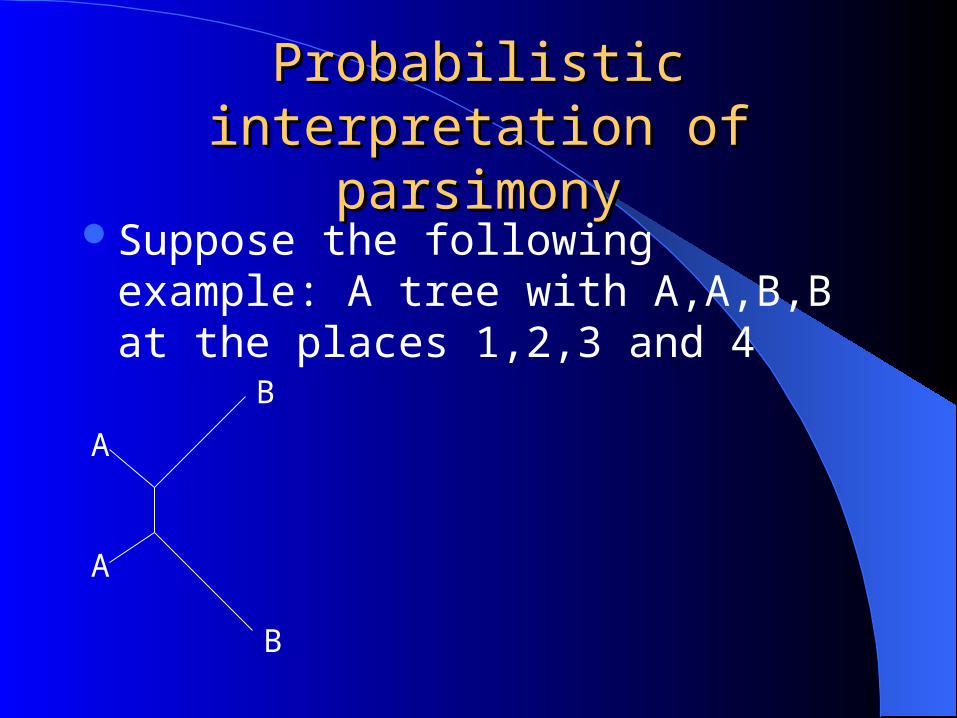
Suppose the following example: A tree with A,A,B,B at the places 1,2,3 and 4
A
A
B
B
Probabilistic interpretation of Probabilistic interpretation of parsimonyparsimony
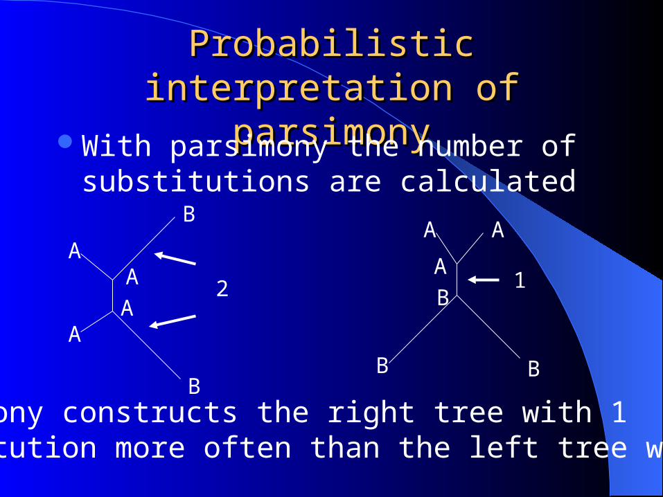
With parsimony the number of substitutions are calculated
A A
B B
A
A
B
B
A
A
A
B2 1
Parsimony constructs the right tree with 1 substitution more often than the left tree with 2

Maximum Likelihood distancesMaximum Likelihood distances
Suppose tree T, edge lengths and sampled sequences at the leafs
We’ll try to compute the distance between and
1x
2x
3x4x 5x
6x
8x
1t 3t
6t 7t
4t
7x
nttt ,,1 ix
1x3x

By multiplicativety
Maximum Likelihood distancesMaximum Likelihood distances
1x
2x
3x4x 5x
6x
8x
1t 3t
6t 7t
4t
7x
6
),|(),|(),|( 686
161
6181
a
taaPtaaPttaaP

8
8),|(),|( 3783
6181
aa
qttaaPttaaP
By reversibility and multiplicativity
1x
2x
3x4x 5x
6x
8x
1t 3t
6t 7t
4t
7x
1x3x
61 tt 37 tt
1x
3x
3761 tttt
3
8
3
),|(
),|(),|(
736131
7338
6181
a
aa
qttttaaP
qttaaPttaaP

u
ju
iux
t
MLij txxPqd j
u),|(maxarg
u
ju
iu
t
MLij txxPd ),|(maxarg
),|(),|,(1 r
ju
kkj
uiux
ju
iu ttxxPqtTxxP
Maximum Likelihood distancesMaximum Likelihood distances

Maximum Likelihood distancesMaximum Likelihood distances
ML distances between leaf sequences are close to additive, given large amount of data
rkkMLij ttd
1
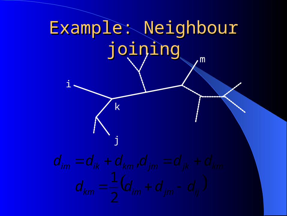
Example: Neighbour joiningExample: Neighbour joining
i
j
k
m
kmjkjmkmikim dddddd ,
ijjmimkm dddd 2
1

Example: Neighbour joiningExample: Neighbour joining
Use Maximum Likelihood distancesSuppose we have a multiplicative reversible
modelSuppose we have plenty of data The underlying probabilistic model is
correctThen Neighbour joining will construct any
tree correctly.

Example: Neighbour joiningExample: Neighbour joining Neighbour joining using ML distances
It constructs the correct tree where Parsimony failed
N
20 477 301 222
100 635 231 134
500 896 85 19
2000 997 5 0
1T 2T 3T

More probabilistic interpretationsMore probabilistic interpretationsSankoff & Cedergren
– Simultaneously aligning sequences and finding its phylogeny, by using a character substitution model
– Probabilistic when scores are interpreted as log probabilities and if the procedure is additive in stead of maximizing.
Allison, Wallace & Yee [1992] – But as the original S&C method it is not
practical for most problems.

More probabilistic interpretationsMore probabilistic interpretationsHein’s affine cost algorithm
– Simultaneously aligning sequences and finding its phylogeny, by using affine gap penalties
– Probabilistic when scores are interpreted as log probabilities and if the procedure is additive in stead of maximizing.
– But when using plus in stead of max we have to include all the paths, which will cost at the first node above the leaf and at the next and so on. So all the speed advantages are gone.
2N3N

ConclusionConclusion Probabilistic interpretations can be better
– Compare ML with parsimony They can also be less useful, because of costs
which get too high– Sankoff & Cedergren
Neighbour joining constructs the correct tree if it has the correct assumptions
So, the trick is to know your problem and to decide which method is the best
Questions??
Related Documents