Real-Time Takagi–Sugeno Fuzzy Control of a Robot Manipulator Ramon Garcia-Hernandez, 1,∗ Jose A. Ruz-Hernandez, 1,† Edgar N. Sanchez, 2,‡ Victor Santiba ˜ nez, 3,§ Miguel A. Llama 3,¶ 1 Universidad Autonoma del Carmen, Calle 56 # 4 Esq. Avenida Concordia, C.P.24180, Colonia Aviacion, Cd. del Carmen, Campeche, Mexico 2 CINVESTAV, Unidad Guadalajara, Apartado Postal 31-430, Plaza La Luna, C.P. 62490, Guadalajara, Jalisco, Mexico 3 Instituto Tecnologico de la Laguna, Apartado Postal 49, Adm. 1, C.P. 27001, Torreon, Coahuila, Mexico This paper presents the development of a control algorithm, which combines the linear regulator theory and Takagi–Sugeno (T–S) fuzzy modeling. Each local controller consists in a feedback control term plus a trajectory tracking term. The global controller is determined by means of T–S methodology. Then, the proposed algorithm is applied in real time on a robot manipulator. C 2009 Wiley Periodicals, Inc. 1. INTRODUCTION The Takagi–Sugeno (T–S) fuzzy approach 1 has been used for identification and control of nonlinear systems. Using this technique, the dynamic of a nonlinear system is easily obtained by linearization at different operation points or (if this model is not well known) by input–output identification around these points. Once these linear models are obtained, local linear controller can be designed; the overall controller would be a fuzzy blending of these controllers. In Ref. 2, an iterative procedure for designing stable T–S fuzzy control is proposed, which is based on finding a common positive definite matrix satisfying the associated Lyapunov equations of locals models. To avoid this iterative process, synthesis of fuzzy T–S controllers is directly obtained by minimization of a linear performance index under linear matrix ∗ Author to whom all correspondence should be addressed: e-mail: rghernandez@pampano. unacar.mx. † e-mail: [email protected]. ‡ e-mail: [email protected]. § e-mail: [email protected]. ¶ e-mail: [email protected]. INTERNATIONAL JOURNAL OF INTELLIGENT SYSTEMS, VOL. 24, 1174–1201 (2009) C 2009 Wiley Periodicals, Inc. Published online in Wiley InterScience (www.interscience.wiley.com). • DOI 10.1002/int.20380

Welcome message from author
This document is posted to help you gain knowledge. Please leave a comment to let me know what you think about it! Share it to your friends and learn new things together.
Transcript
Real-Time Takagi–Sugeno Fuzzy Control ofa Robot ManipulatorRamon Garcia-Hernandez,1,∗ Jose A. Ruz-Hernandez,1,†
Edgar N. Sanchez,2,‡ Victor Santibanez,3,§ Miguel A. Llama3,¶
1Universidad Autonoma del Carmen, Calle 56 # 4 Esq. Avenida Concordia,C.P. 24180, Colonia Aviacion, Cd. del Carmen, Campeche, Mexico2CINVESTAV, Unidad Guadalajara, Apartado Postal 31-430, Plaza La Luna,C.P. 62490, Guadalajara, Jalisco, Mexico3Instituto Tecnologico de la Laguna, Apartado Postal 49, Adm. 1, C.P. 27001,Torreon, Coahuila, Mexico
This paper presents the development of a control algorithm, which combines the linear regulatortheory and Takagi–Sugeno (T–S) fuzzy modeling. Each local controller consists in a feedbackcontrol term plus a trajectory tracking term. The global controller is determined by means of T–Smethodology. Then, the proposed algorithm is applied in real time on a robot manipulator. C© 2009Wiley Periodicals, Inc.
1. INTRODUCTION
The Takagi–Sugeno (T–S) fuzzy approach1 has been used for identification andcontrol of nonlinear systems. Using this technique, the dynamic of a nonlinear systemis easily obtained by linearization at different operation points or (if this model is notwell known) by input–output identification around these points. Once these linearmodels are obtained, local linear controller can be designed; the overall controllerwould be a fuzzy blending of these controllers. In Ref. 2, an iterative procedurefor designing stable T–S fuzzy control is proposed, which is based on finding acommon positive definite matrix satisfying the associated Lyapunov equations oflocals models. To avoid this iterative process, synthesis of fuzzy T–S controllers isdirectly obtained by minimization of a linear performance index under linear matrix
∗Author to whom all correspondence should be addressed: e-mail: [email protected].
†e-mail: [email protected].‡e-mail: [email protected].§e-mail: [email protected].¶e-mail: [email protected].
INTERNATIONAL JOURNAL OF INTELLIGENT SYSTEMS, VOL. 24, 1174–1201 (2009)C© 2009 Wiley Periodicals, Inc. Published online in Wiley InterScience
(www.interscience.wiley.com). • DOI 10.1002/int.20380
REAL-TIME TAKAGI–SUGENO FUZZY CONTROL OF A ROBOT MANIPULATOR 1175
inequalities (LMIs) constrains; solving this optimization problem, the resultingfuzzy controller exhibits stability and performance.3−5
Nonlinear system trajectory tracking based on T–S fuzzy approach, which ismore difficult than set point regulation, has been less analyzed. In Ref. 6, trackingis achieved by minimizing the error between the nonlinear system and a nonlinearreference model, then the error is minimized and closed-loop stability conditions areestablished by means of LMIs. A T–S scheme for real-time trajectory tracking of anunderactuated robot is described in Ref. 7. The results obtained using this schemeare quite encouraging to track sinusoidal signals of big amplitude.
In Ref. 8, a stable neuro-fuzzy adaptive control approach for the trajectorytracking of the robotic manipulators with poorly known dynamics is proposed. Thefuzzy dynamic model of the manipulator is obtained via T–S fuzzy methodology. Adynamic neuro-fuzzy adaptive controller is developed to improve the system perfor-mance by adaptively modifying the fuzzy model parameters online. Furthermore, thesystem stability and the convergence of tracking errors are guaranteed by Lyapunovstability theory. Other application for robotic manipulators is described in Ref. 9. Inthis application, a technique is proposed to adaptively tune a sliding mode controllergain via a fuzzy logic system as adaptation mechanism. The proposed controllerachieves a high performance with minimum reaching time and smooth control ac-tions. In Ref. 10, a sliding-mode neural-network control scheme for the trackingcontrol of an n-rigid link robot manipulator is developed to achieve high-precisionposition control. The scheme guarantees the stability of controlled system and noconstrained conditions and prior knowledge of the controlled plant are required inthe design process. However, all these publications include only simulation results.
An interesting investigation and development of a fuzzy control highly nonlin-ear two-axis manipulator with a single-flexible link using a novel patented optical tipdisplacement feedback is described in Ref. 11. The controller comprises a parallelfuzzy supervisor that is used to alter the derivative term of a linear classical Propor-tional Derivative (PD) controller, which is updated in relation to the measured tiperror and error rate. Implementation of the supervisory fuzzy controller is describedusing both serial and parallel operation transputers.
An alternative approach to trajectory tracking for a robot manipulator is pro-posed in this paper. As in Ref. 7, the approach combines linear regulator theory andT–S fuzzy method to design a tracking controller. The viability of this approach isillustrated via successful real-time results for a two degrees of freedom robot manip-ulator. The originality of this paper is mainly related to the real-time implementationof the proposed T–S fuzzy control algorithm.
2. T–S FUZZY CONTROL ALGORITHM
In this section as in Ref. 7, we present the used T–S fuzzy control schemefor nonlinear system trajectory tracking as well as some well-known preliminariesabout T–S model and linear regulator theory.
International Journal of Intelligent Systems DOI 10.1002/int
1176 GARCIA-HERNANDEZ ET AL.
2.1. T–S Fuzzy Model
In this approach, nonlinear systems are approximated by a set of linear localmodels. A dynamic T–S fuzzy model1 is described by a set of “IF-THEN” rules asfollows:
ith Rule:
IF z1(t) is Mi1, . . . , zj (t) is Mij , . . . , zq(t) is Miq
THEN{
x(t) = Aix(t) + Biu(t)y(t) = Cix(t)
where i = 1, . . . , r with r the number of rules; zj (j = 1, . . . , q) premise variables,which may be functions of the states or the other variables; Mij fuzzy sets; x ∈ �n
state vector; u ∈ �m input vector; y ∈ �p output vector; and Ai , Bi , and Ci matricesof adequate dimension. We will denote z(t) as the vector containing all the zj .
The final state and output of the fuzzy system is inferred as
x(t) =∑r
i=1 λi(z(t)) {Aix(t) + Biu(t)}∑ri=1 λi(z(t))
y(t) =∑r
i=1 λi(z(t)) {Cix(t)}∑ri=1 λi(z(t))
(1)
where λi(z(t)) = ∑q
j=1 μij and μij is the membership function of zj (t) in Mij .
2.2. Linear Regulator
In linear regulator theory,12 the control goal is to obtain a stable closed-loopsystem and asymptotic tracking error for every possible initial state and everypossible exogenous input in a prescribed family of functions of time. This latterrequirement is also known as the property of “output regulation.”
Let us consider a linear system
x(t) = Ax(t) + Bu(t) + Pw(t)w(t) = Sw(t) (2)e(t) = Cx(t) + Qw(t)
where x(t) ∈ �n is the internal state vector of the plant; u(t) ∈ �m denotes thecontrol input vector; w(t) ∈ �q is the vector containing external disturbances and/orreferences; and e(t) is the tracking error.To solve this problem, the following assumptions are considered.
H1: The pair (A, B) is stabilizable.H2: The exosystem is antistable, that is, all the eigenvalues of S have nonneg-
ative real part.
International Journal of Intelligent Systems DOI 10.1002/int
REAL-TIME TAKAGI–SUGENO FUZZY CONTROL OF A ROBOT MANIPULATOR 1177
Assuming H1 and H2, the problem of output regulation via state feedback can bedetermined only if there exist matrices � and �, which solve the following linearmatrix equations:
�S = A� + B� + P
0 = C� + Q(3)
The control law is given as u(t) = Kx(t) + (� − K�)w(t) with K any matrixsuch that (A + BK) is Hurwitz. Defining L =� −K�, we have
u(t) = Kx(t) + Lw(t) (4)
2.3. T–S Algorithm
At this stage, we present the used T–S fuzzy control for nonlinear systemtrajectory tracking. For the controller rules, we use as antecedents the same fuzzysets used in the plant rules. As consequents, we design local control laws based onthe linear regulator theory for each local linear model. The rules for the plant andcontroller are
ith Plant Rule:
IF z1(t) is Mi1, . . . , zj (t) is Mij , . . . , zq(t) is Miq
THEN
⎧⎨⎩
x(t) = Aix(t) + Biu(t) + Piw(t)w(t) = Sw(t)e(t) = Cix(t) + Qiw(t)
(5)
ith Controller Rule:
IF z1(t) is Mi1, . . . , zj (t) is Mij , . . . , zq(t) is Miq
THEN u(t) = Kix(t) + Liw(t)(6)
where Ki is any matrix such that (Ai +BiKi) is Hurwitz; �i and �i satisfyEquation 3 for each (Ai , Bi , Ci , Pi , S, Qi); i = 1, . . . , r .
The output of the fuzzy controller is given as
u(t) =∑r
i=1 λi(z(t)) [Kix(t) + Liw(t)]∑ri=1 λi(z(t))
(7)
3. STABILITY AND TRACKING ANALYSIS
This section contains the mathematical preliminaries about the stability andtracking analysis, which are taken into account to design the fuzzy controller de-scribed in Section 4.2.
International Journal of Intelligent Systems DOI 10.1002/int
1178 GARCIA-HERNANDEZ ET AL.
3.1. Stability Analysis
To check stability of the fuzzy system, we must find a common positive definitematrix P, such that conditions of the next theorem are satisfied.
THEOREM 3.1.13 The closed-loop fuzzy control system is globally asymptoticallystable if there exists a common positive definite matrix P such that
(Ai − BiKi)T P + P(Ai − BiKi) < 0
for i = 1, . . . , r and
((Ai − BiKj ) + (Aj − BjKi))T
2P + P
((Ai − BiKj ) + (Aj − BjKi))
2≤ 0
for i, j = 1, . . . , r
where Ai and Bi are the matrices of local linear models and Ki denote the feedbackmatrices.
3.2. Tracking Analysis
The following results are taken from Ref. 14. The regulator problem solutionfor linear subsystems would be inferred from the existence of a solution to the matrixequations
�iSi = Ai�i + Bi�i + Pi
0 = Ci�i + Qi(8)
for each subsystem. Unfortunately, this fact is generally not true. At this point, theseequations would solve the regulation problem for the overall nonlinear setting if andonly if the following equations hold:
0 =r∑
i=1
μi�i +r−1∑i=1
r∑j=i+1
μiμj (�iSj + �jSi)
−r−1∑i=1
r∑j=i+1
μiμj (Ai�j + Bi�j + Pi + Aj�i + Bj�i + Pj )
0 =r−1∑i=1
r∑j=i+1
μiμj (Ci�j + Qi + Cj�i + Qj )
which are in general not true. However, a particular case occurs when �1 =�2 = · · ·= �r = �. Then, the term
∑ri=1 μi�i = ∑r
i=1 μi� = 0 since∑r
i=1 μi = 1. Thus,
International Journal of Intelligent Systems DOI 10.1002/int
REAL-TIME TAKAGI–SUGENO FUZZY CONTROL OF A ROBOT MANIPULATOR 1179
the equation Ci� + Qi + Cj� + Qj = 0 is trivially satisfied by Equation 8 and weonly need to satisfy
0 =r−1∑i=1
r∑j=i+1
μiμj (�Sj + �Si)
−r−1∑i=1
r∑j=i+1
μiμj (Ai� + Bi�j + Pi + Aj� + Bj�i + Pj )
(9)
Now, we can distinguish two cases:(a) B1 = B2 = · · · = Br = B.
(b) �1 = �2 = · · · = �r = �.
In both cases, Equation 9 is trivially satisfied by Equation 8 and then theregulator problem is solvable. Corollaries that resume the previous discussion canbe reviewed in Ref. 14.
Furthermore, in Ref. 15, a methodology is presented to bound the trackingerror for the overall fuzzy model. A real positive value β is found such that theoverall steady-state error e(t) satisfies ‖e(t)‖ < β(t). However, this approach doesnot consider the case when �1 =�2 = · · · = �r = � are all equals and then β iszero.
4. EXPERIMENTAL CASE STUDY
4.1. Robot Description
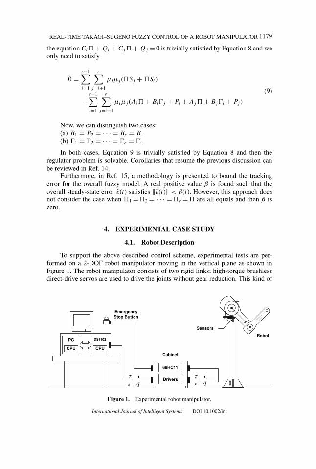
To support the above described control scheme, experimental tests are per-formed on a 2-DOF robot manipulator moving in the vertical plane as shown inFigure 1. The robot manipulator consists of two rigid links; high-torque brushlessdirect-drive servos are used to drive the joints without gear reduction. This kind of
CPU CPU
PC DS1102
EmergencyStop Button
Sensors
Cabinet
68HC11
Driversτ
q qτ
Robot
⋅
Figure 1. Experimental robot manipulator.
International Journal of Intelligent Systems DOI 10.1002/int
1180 GARCIA-HERNANDEZ ET AL.
joints presents reduced backlash and significantly lower joint friction as compared toactuators with gear drives. The motors used in the experimental arm are DM1200-Aand DM1015-B from Parker Compumotor, for the shoulder and elbow joints, respec-tively. For this application, the servos are operated in “torque mode,” so the motorsact as torque sources and accept an analog voltage as a reference of torque signal. Inthis configuration, the motor DM1200-A is capable of delivering a maximum torqueof 150 N·m and the motor DM1015-B delivers only 15 N·m. Angular information isobtained from incremental encoders located on the motors, which have a resolutionof 1,024,000 pulses/rev for the first motor and 655,300 for the second one (accuracy0.0069◦ for both motors), and the angular velocity information is computed vianumerical differentiation of the angular position signal.
The control program is written in C programming language of the TMS320compiler for the TMS320C31 32-bit floating point microprocessor from Texas In-struments. The control algorithm is executed at 25 ms rate in a control board DS1102from DSpace, based on the same microprocessor. This board is mounted in a IBM-compatible 486 processor, 66-MHz host computer.16
Experiments show that Coulomb friction and viscous friction at the motor jointsare present and depend, in a complex manner, on the joint position and velocity.Instead of modeling these friction phenomena for compensation purposes, we havedecided to consider them as unmodeled dynamics.
The dynamics of an n-link rigid robot, including the effect of viscous friction,can be written as17:
M(q)q + C(q, q)q + g(q) + f (q) = τ (10)
where q is the n× 1 vector displacements, q is the n× 1 vector of joint velocities,τ is the n× 1 vector of applied torques, M(q) is the n× n symmetric positive def-inite manipulator inertia matrix, C(q, q) is n× n matrix of centripetal and Coriolistorques, g(q) is n× 1 vector of gravitational torques obtained as the gradient of therobot potential energy due to gravity, and f (q) denotes the n× 1 vector of viscousfriction coefficients.
The equation of motion for the robot can be formulated as a nonlinear state–space description x(t) = f (x) + g(x)u(t), where x(t) = [q1 q2 q1 q2]T is the statevector and u(t) = [τ1 τ2]T is the input vector (τ1 and τ2 are torques applied to link1 and link 2, respectively).
Linearization of this nonlinear model for specific equilibrium point can beobtaining using Taylor series; hence, the respective linearization is given as x(t) =Ax(t) + Bu(t), where
A := ∂F (x(t), u(t), t)
∂x
∣∣∣∣x0,u0
B := ∂F (x(t), u(t), t)
∂u
∣∣∣∣x0,u0
and xo = [qo1 qo
2 qo1 qo
2 ]T , uo = [τ o1 τ o
2 ]T are the values of x and u for the specificequilibrium point.
International Journal of Intelligent Systems DOI 10.1002/int
REAL-TIME TAKAGI–SUGENO FUZZY CONTROL OF A ROBOT MANIPULATOR 1181
1
0 1
Z1
Radians
PN
x
( )xμ
Radians
PN( )xμ
x
)b()a(
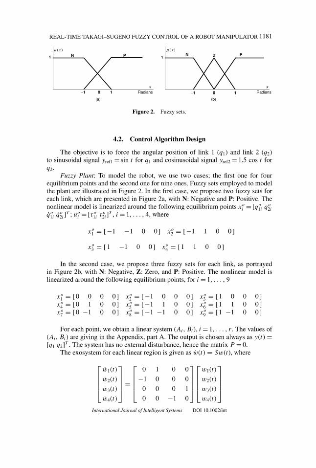
Figure 2. Fuzzy sets.
4.2. Control Algorithm Design
The objective is to force the angular position of link 1 (q1) and link 2 (q2)to sinusoidal signal yref1 = sin t for q1 and cosinusoidal signal yref2 = 1.5 cos t forq2.
Fuzzy Plant: To model the robot, we use two cases; the first one for fourequilibrium points and the second one for nine ones. Fuzzy sets employed to modelthe plant are illustrated in Figure 2. In the first case, we propose two fuzzy sets foreach link, which are presented in Figure 2a, with N: Negative and P: Positive. Thenonlinear model is linearized around the following equilibrium points xo
i = [qo1i qo
2i
qo1i qo
2i]T ; uo
i = [τ o1i τ o
2i]T , i = 1, . . . , 4, where
xo1 = [−1 −1 0 0 ] xo
2 = [−1 1 0 0 ]
xo3 = [ 1 −1 0 0 ] xo
4 = [ 1 1 0 0 ]
In the second case, we propose three fuzzy sets for each link, as portrayedin Figure 2b, with N: Negative, Z: Zero, and P: Positive. The nonlinear model islinearized around the following equilibrium points, for i = 1, . . . , 9
xo1 = [ 0 0 0 0 ] xo
2 = [−1 0 0 0 ] xo3 = [ 1 0 0 0 ]
xo4 = [ 0 1 0 0 ] xo
5 = [−1 1 0 0 ] xo6 = [ 1 1 0 0 ]
xo7 = [ 0 −1 0 0 ] xo
8 = [−1 −1 0 0 ] xo9 = [ 1 −1 0 0 ]
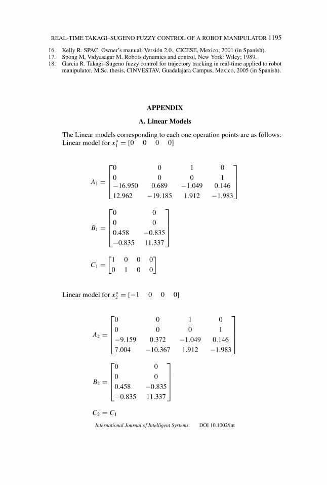
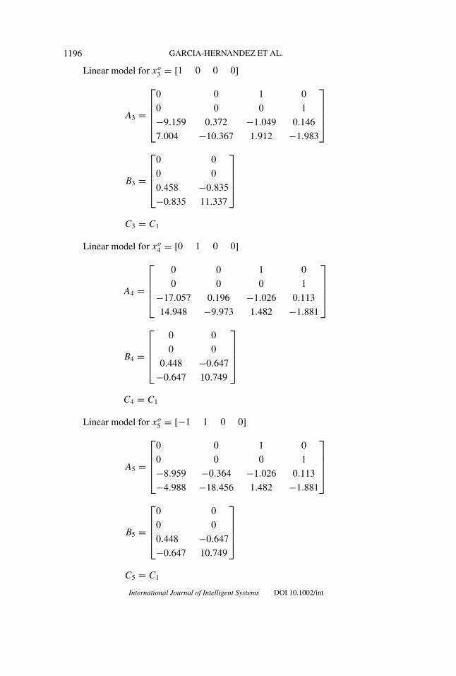
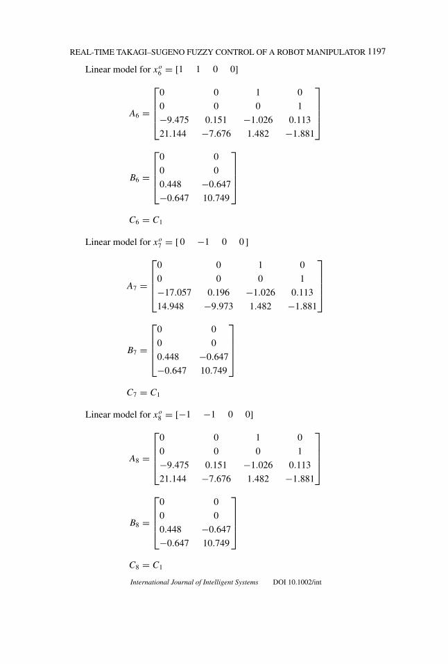
For each point, we obtain a linear system (Ai , Bi), i = 1, . . . , r . The values of(Ai , Bi) are giving in the Appendix, part A. The output is chosen always as y(t) =[q1 q2]T . The system has no external disturbance, hence the matrix P = 0.
The exosystem for each linear region is given as w(t) = Sw(t), where
⎡⎢⎢⎢⎣
w1(t)
w2(t)
w3(t)
w4(t)
⎤⎥⎥⎥⎦ =
⎡⎢⎢⎢⎣
0 1 0 0
−1 0 0 0
0 0 0 1
0 0 −1 0
⎤⎥⎥⎥⎦
⎡⎢⎢⎢⎣
w1(t)
w2(t)
w3(t)
w4(t)
⎤⎥⎥⎥⎦
International Journal of Intelligent Systems DOI 10.1002/int
1182 GARCIA-HERNANDEZ ET AL.
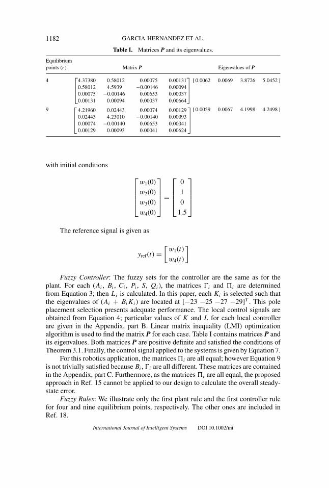
Table I. Matrices P and its eigenvalues.
Equilibriumpoints (r) Matrix P Eigenvalues of P
4 [ 0.0062 0.0069 3.8726 5.0452 ]⎡⎢⎢⎣
4.37380 0.58012 0.00075 0.001310.58012 4.5939 −0.00146 0.000940.00075 −0.00146 0.00653 0.000370.00131 0.00094 0.00037 0.00664
⎤⎥⎥⎦
9 [ 0.0059 0.0067 4.1998 4.2498 ]⎡⎢⎢⎣
4.21960 0.02443 0.00074 0.001290.02443 4.23010 −0.00140 0.000930.00074 −0.00140 0.00653 0.000410.00129 0.00093 0.00041 0.00624
⎤⎥⎥⎦
with initial conditions
⎡⎢⎢⎢⎣
w1(0)
w2(0)
w3(0)
w4(0)
⎤⎥⎥⎥⎦ =
⎡⎢⎢⎢⎣
0
1
0
1.5
⎤⎥⎥⎥⎦
The reference signal is given as
yref(t) =[
w1(t)
w4(t)
]
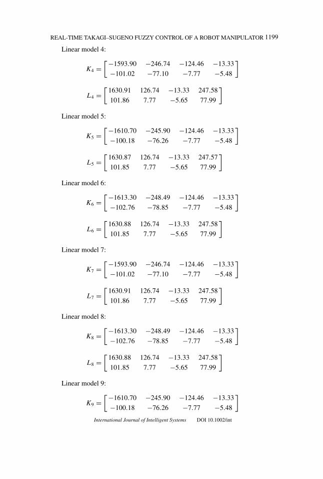
Fuzzy Controller: The fuzzy sets for the controller are the same as for theplant. For each (Ai , Bi , Ci , Pi , S, Qi), the matrices �i and �i are determinedfrom Equation 3; then Li is calculated. In this paper, each Ki is selected such thatthe eigenvalues of (Ai + BiKi) are located at [−23 −25 −27 −29]T . This poleplacement selection presents adequate performance. The local control signals areobtained from Equation 4; particular values of K and L for each local controllerare given in the Appendix, part B. Linear matrix inequality (LMI) optimizationalgorithm is used to find the matrix P for each case. Table I contains matrices P andits eigenvalues. Both matrices P are positive definite and satisfied the conditions ofTheorem 3.1. Finally, the control signal applied to the systems is given by Equation 7.
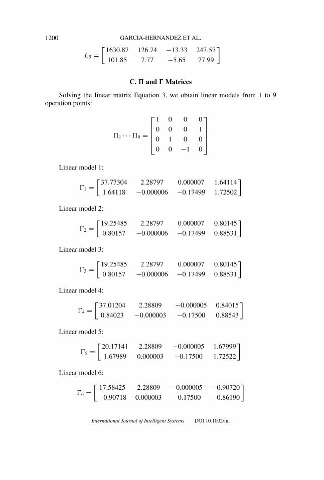
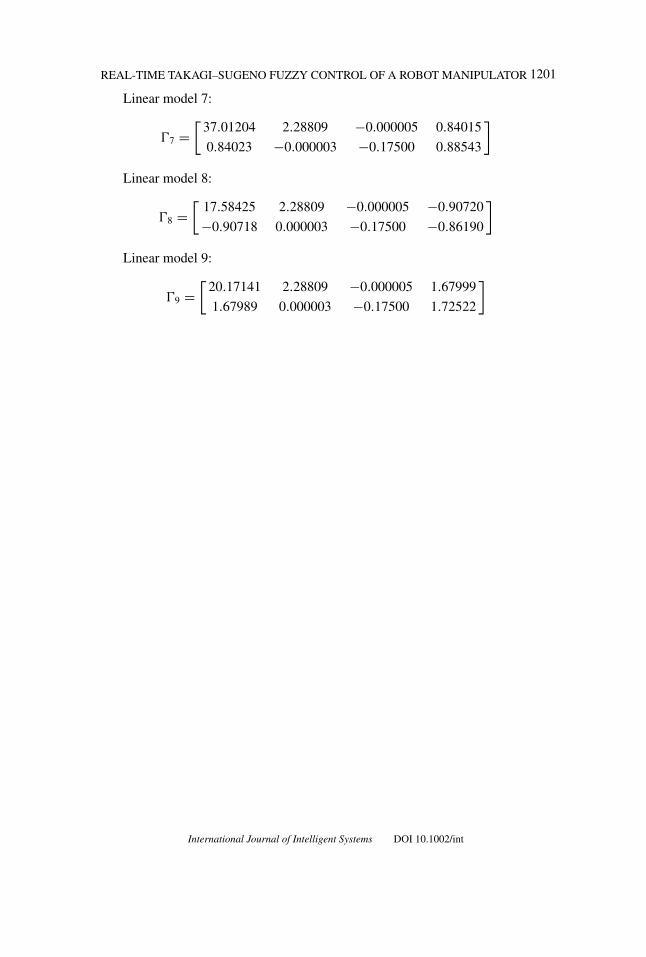
For this robotics application, the matrices �i are all equal; however Equation 9is not trivially satisfied because Bi , �i are all different. These matrices are containedin the Appendix, part C. Furthermore, as the matrices �i are all equal, the proposedapproach in Ref. 15 cannot be applied to our design to calculate the overall steady-state error.
Fuzzy Rules: We illustrate only the first plant rule and the first controller rulefor four and nine equilibrium points, respectively. The other ones are included inRef. 18.
International Journal of Intelligent Systems DOI 10.1002/int
REAL-TIME TAKAGI–SUGENO FUZZY CONTROL OF A ROBOT MANIPULATOR 1183
1st Plant Rule (four equilibrium points):
IF x1(t) is N and x2(t) is N
THEN
⎧⎨⎩
x(t) = A1x(t) + B1u(t)w(t) = Sw(t)e(t) = C1x(t) + Q1w(t)
1st Controller Rule (four equilibrium points):
IF x1(t) is N and x2(t) is NTHEN u(t) = K1x(t) + L1w(t)
1st Plant Rule (nine equilibrium points):
IF x1(t) is Z and x2(t) is Z
THEN
⎧⎨⎩
x(t) = A1x(t) + B1u(t)w(t) = Sw(t)e(t) = C1x(t) + Q1w(t)
1st Controller Rule (nine equilibrium points):
IF x1(t) is Z and x2(t) is ZTHEN u(t) = K1x(t) + L1w(t)
Both designs are implemented via computer simulation. The robot manipulatormodel given as in Equation 10 is used as the plant. The initial conditions for link 1and link 2 angular positions are equal to zero.
4.3. Simulations Results
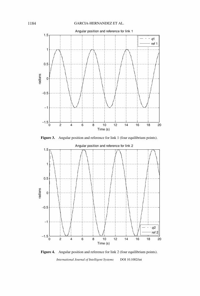
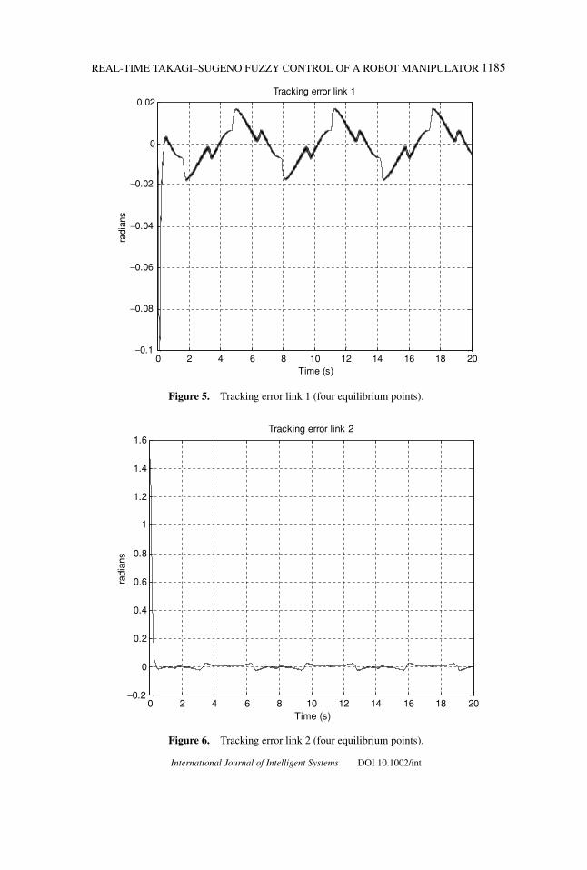
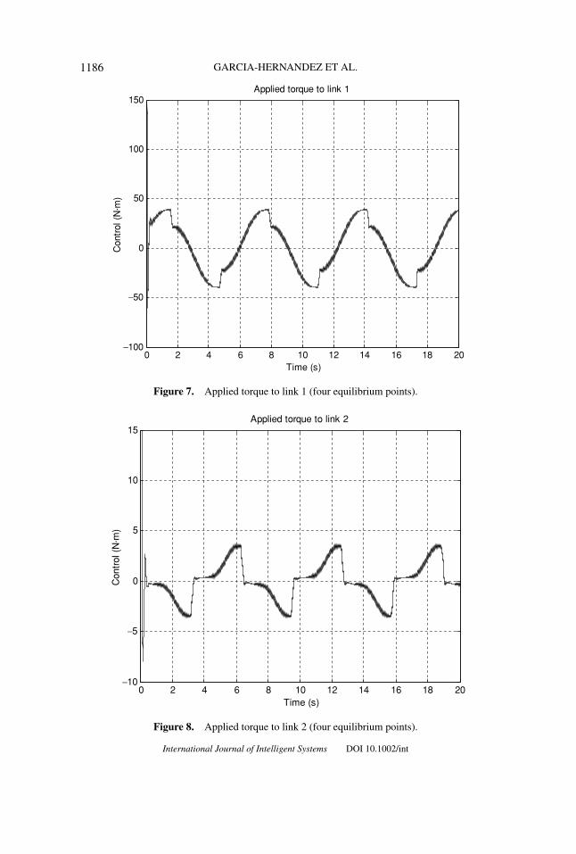
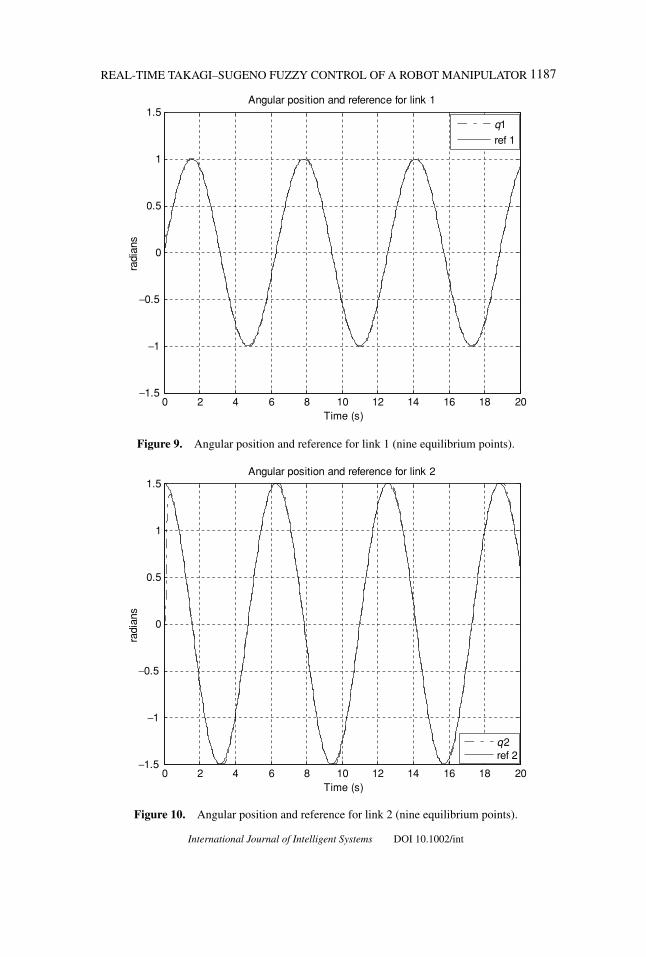
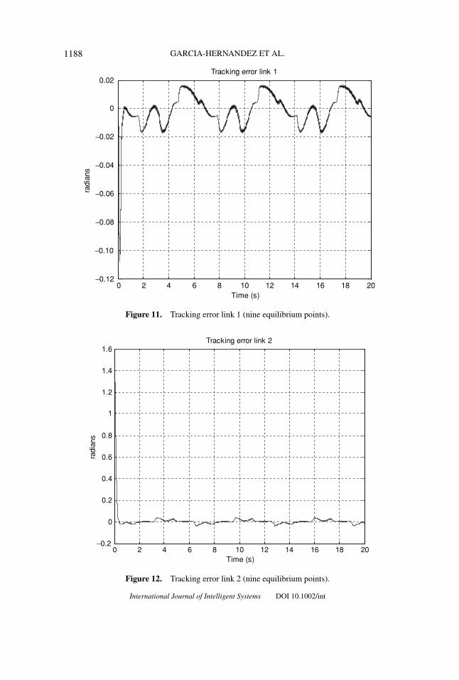
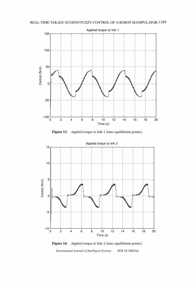
The developed control algorithms are applied via simulation. Figures 3–8 il-lustrate tracking trajectories, tracking errors, and applied torques when four equilib-rium points are used. Figures 9–14 illustrate the same signals using nine equilibriumpoints. Similar simulation results are obtained for both cases.
The following table contains performance indexes for simulation tracking errorsbased on the 2-norm (Table II)
International Journal of Intelligent Systems DOI 10.1002/int
1184 GARCIA-HERNANDEZ ET AL.
0 2 4 6 8 10 12 14 16 18 20−1.5
−1
−0.5
0
0.5
1
1.5
Time (s)
radi
ans
Angular position and reference for link 1
q1
ref 1
Figure 3. Angular position and reference for link 1 (four equilibrium points).
0 2 4 6 8 10 12 14 16 18 20
0
0.5
1
1.5
Time (s)
radi
ans
Angular position and reference for link 2
q 2ref 2
Figure 4. Angular position and reference for link 2 (four equilibrium points).
International Journal of Intelligent Systems DOI 10.1002/int
REAL-TIME TAKAGI–SUGENO FUZZY CONTROL OF A ROBOT MANIPULATOR 1185
0 2 4 6 8 10 12 14 16 18 20
0
0.02
Time (s)
radi
ans
Tracking error link 1
Figure 5. Tracking error link 1 (four equilibrium points).
0 2 4 6 8 10 12 14 16 18 20
0
0.2
0.4
0.6
0.8
1
1.2
1.4
1.6
Time (s)
radi
ans
Tracking error link 2
Figure 6. Tracking error link 2 (four equilibrium points).
International Journal of Intelligent Systems DOI 10.1002/int
1186 GARCIA-HERNANDEZ ET AL.
0 2 4 6 8 10 12 14 16 18 20
0
50
100
150
Time (s)
Con
trol
(N
. m)
Applied torque to link 1
Figure 7. Applied torque to link 1 (four equilibrium points).
0 2 4 6 8 10 12 14 16 18 20
0
5
10
15
Time (s)
Con
trol
(N
. m)
Applied torque to link 2
Figure 8. Applied torque to link 2 (four equilibrium points).
International Journal of Intelligent Systems DOI 10.1002/int
REAL-TIME TAKAGI–SUGENO FUZZY CONTROL OF A ROBOT MANIPULATOR 1187
0 2 4 6 8 10 12 14 16 18 20
0
0.5
1
1.5
Time (s)
radi
ans
Angular position and reference for link 1
q1
ref 1
Figure 9. Angular position and reference for link 1 (nine equilibrium points).
0 2 4 6 8 10 12 14 16 18 20
0
0.5
1
1.5
Time (s)
radi
ans
Angular position and reference for link 2
q2ref 2
Figure 10. Angular position and reference for link 2 (nine equilibrium points).
International Journal of Intelligent Systems DOI 10.1002/int
1188 GARCIA-HERNANDEZ ET AL.
0 2 4 6 8 10 12 14 16 18 20
0
0.02
Time (s)
radi
ans
Tracking error link 1
Figure 11. Tracking error link 1 (nine equilibrium points).
0 2 4 6 8 10 12 14 16 18 20
0
0.2
0.4
0.6
0.8
1
1.2
1.4
1.6
Time (s)
radi
ans
Tracking error link 2
Figure 12. Tracking error link 2 (nine equilibrium points).
International Journal of Intelligent Systems DOI 10.1002/int
REAL-TIME TAKAGI–SUGENO FUZZY CONTROL OF A ROBOT MANIPULATOR 1189
0 2 4 6 8 10 12 14 16 18 20
0
50
100
150
Time (s)
Con
trol
(N
. m)
Applied torque to link 1
Figure 13. Applied torque to link 1 (nine equilibrium points).
0 2 4 6 8 10 12 14 16 18 20
0
5
10
15
Time (s)
Con
trol
(N
. m)
Applied torque to link 2
Figure 14. Applied torque to link 2 (nine equilibrium points).
International Journal of Intelligent Systems DOI 10.1002/int
1190 GARCIA-HERNANDEZ ET AL.
Table II. Performance indexes for simulation tracking errors.
Number ofequilibrium points (r) ‖e1(t)‖2 ‖e2(t)‖2 ‖e1(t)‖2 + ‖e2(t)‖2 Units
4 1.4861 15.5207 17.0068 rad9 1.5971 15.6377 17.2348 rad
where
e1(t) = q1(t) − w1(t) (11)
and
e2(t) = q2(t) − w4(t) (12)
4.4. Real-Time Results
Even if the simulation results are almost identified for four equilibrium pointsand for nine ones, we decide to implement in real time the last case. The main reasonto take this decision is due to the fact that for simulations, friction is not considered;from our point of view, the more equilibrium points are used the better robustnessin presence of friction is obtained.
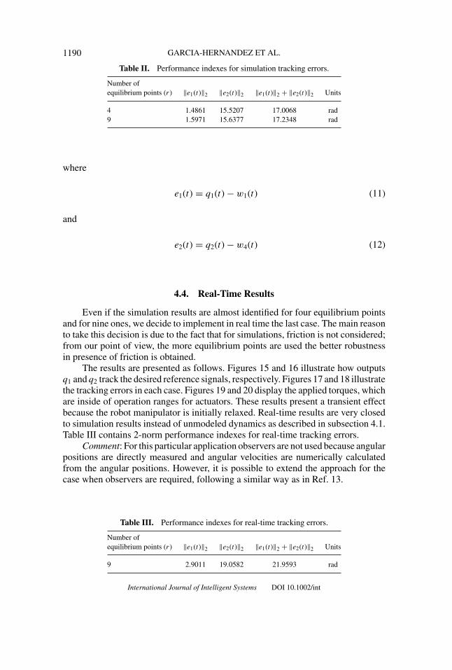
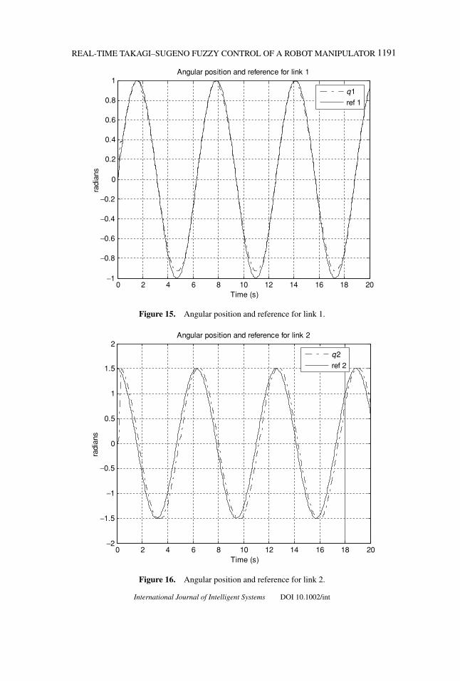
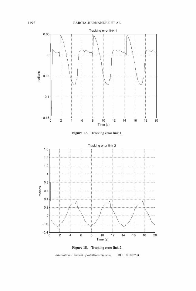
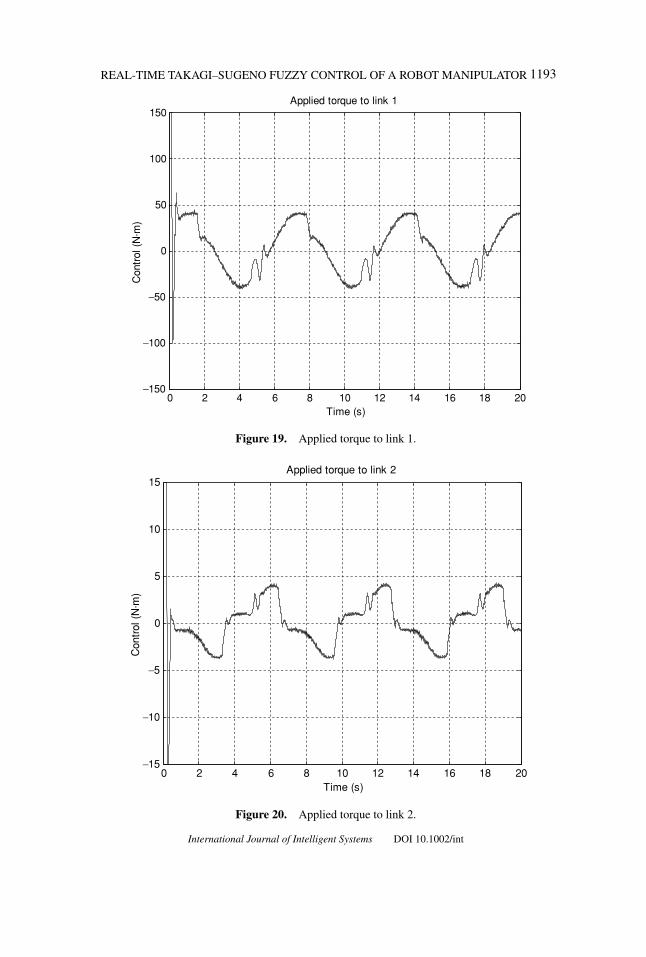
The results are presented as follows. Figures 15 and 16 illustrate how outputsq1 and q2 track the desired reference signals, respectively. Figures 17 and 18 illustratethe tracking errors in each case. Figures 19 and 20 display the applied torques, whichare inside of operation ranges for actuators. These results present a transient effectbecause the robot manipulator is initially relaxed. Real-time results are very closedto simulation results instead of unmodeled dynamics as described in subsection 4.1.Table III contains 2-norm performance indexes for real-time tracking errors.
Comment: For this particular application observers are not used because angularpositions are directly measured and angular velocities are numerically calculatedfrom the angular positions. However, it is possible to extend the approach for thecase when observers are required, following a similar way as in Ref. 13.
Table III. Performance indexes for real-time tracking errors.
Number ofequilibrium points (r) ‖e1(t)‖2 ‖e2(t)‖2 ‖e1(t)‖2 + ‖e2(t)‖2 Units
9 2.9011 19.0582 21.9593 rad
International Journal of Intelligent Systems DOI 10.1002/int
REAL-TIME TAKAGI–SUGENO FUZZY CONTROL OF A ROBOT MANIPULATOR 1191
0 2 4 6 8 10 12 14 16 18 20
0
0.2
0.4
0.6
0.8
1
Time (s)
radi
ans
Angular position and reference for link 1
q1
ref 1
Figure 15. Angular position and reference for link 1.
0 2 4 6 8 10 12 14 16 18 20
0
0.5
1
1.5
2
Time (s)
radi
ans
Angular position and reference for link 2
q2
ref 2
Figure 16. Angular position and reference for link 2.
International Journal of Intelligent Systems DOI 10.1002/int
1192 GARCIA-HERNANDEZ ET AL.
0 2 4 6 8 10 12 14 16 18 20
0
0.05
Time (s)
radi
ans
Tracking error link 1
Figure 17. Tracking error link 1.
0 2 4 6 8 10 12 14 16 18 20
0
0.2
0.4
0.6
0.8
1
1.2
1.4
1.6
Time (s)
radi
ans
Tracking error link 2
Figure 18. Tracking error link 2.
International Journal of Intelligent Systems DOI 10.1002/int
REAL-TIME TAKAGI–SUGENO FUZZY CONTROL OF A ROBOT MANIPULATOR 1193
0 2 4 6 8 10 12 14 16 18 20
0
50
100
150
Time (s)
Con
trol
(N
. m)
Applied torque to link 1
Figure 19. Applied torque to link 1.
0 2 4 6 8 10 12 14 16 18 20
0
5
10
15
Time (s)
Con
trol
(N
. m)
Applied torque to link 2
Figure 20. Applied torque to link 2.
International Journal of Intelligent Systems DOI 10.1002/int
1194 GARCIA-HERNANDEZ ET AL.
5. CONCLUSIONS
Real-time results demonstrate that proposed algorithm is an adequate mecha-nism for trajectory tracking as applied to a robot manipulator. Even if it is possibleto guarantee stability of the closed loop, the same is not true regarding trackingerrors; this subject rests open as a topic of future research.
Acknowledgments
Ramon Garcia-Hernandez thanks CONACYT for its support via undergraduate scholarshipto carry out his M. Sc. studies. The first and second authors thank Jose L. Rullan-Lara for hisparticipation.
References
1. Takagi T, Sugeno M. Fuzzy identification of systems and its applications to modeling andcontrol. IEEE Trans. Syst Man Cybern 1985;15:116–132.
2. Tanaka K, Sugeno M. Stability analysis and design of fuzzy control system. Fuzzy Sets Syst1992;45:133–156.
3. Jadbabaie A, Jamshidi M, Titli A. Guaranteed-cost design of continuous-time Takagi–Sugeno fuzzy controllers via Linear Matrix Inequalities. In: Proc of the 1998 IEEE WorldCongress on Computational Intelligence, Anchorage, AK, 1998.
4. Hong S, Langari R. Synthesis of an LMI-based fuzzy control system with guaranteed optimalH-infinity performance. In: Proc of the 1998 IEEE World Congress on ComputationalIntelligence, Anchorage, AK, 1998.
5. Tanaka K, Taniguchi T, Wang H. Fuzzy control based on quadratic performance function: Alinear matrix inequality approach. In: Proc of the 1998 IEEE Conference on Decision andControl, Tampa, FL, 1998.
6. Taniguchi T, Tanaka K, Yamafuji K, Wang H. Nonlinear model following control viaTakagi–Sugeno fuzzy model. In: Proc of the American Control Conference, San Diego, CA,1999.
7. Begovich O, Sanchez E, Maldonado M. Takagi–Sugeno fuzzy scheme for real-time trajectorytracking of an underactuated robot. IEEE Trans Control Syst 2002;10(1):14–20.
8. Sun F, Sun Z, Li L, Li H-X. Neuro-fuzzy adaptive control based on dynamic inversion forrobotic manipulators. Fuzzy Sets Syst 2003;134(1):117–133.
9. Abdelhameed M. Enhancement of sliding mode controller by fuzzy logic with applicationto robotic manipulators. Mechatronics 2005;15(4):439–458.
10. Wai R-J. Tracking control based on neural networks strategy for robot manipulator. Neuro-computing 2003;51:425–445.
11. Surdhar J, White A. A parallel fuzzy-controlled flexible manipulator using optical tip feed-back. Rob Comput Integr Manuf 2003;19:273–282.
12. Knobloch H, Isidori A, Flockerzi D. Topics in control theory, Berlin, Germany: Springer-Verlag; 1993.
13. Tanaka K, Wang H. Fuzzy control systems design and analysis. A linear matrix inequalityapproach, New York, Wiley, 2001.
14. Castillo-Toledo B, Meda-Campana J, Titli A. A fuzzy output regulator for Takagi–Sugenofuzzy models. In: Proc of the 2003 IEEE International Symposium on Intelligent Control,Volume 2, Houston, Texas, 2003 pp 310–315.
15. Meda-Campana J, Castillo-Toledo B. The regulation problem for nonlinear time-delay sys-tems using Takagi–Sugeno fuzzy models: An LMI approach. In: Proc of the 2005 IEEEInternational Symposium on Intelligent Control, Limassol, Cyprus; 2005. pp 1045–1050.
International Journal of Intelligent Systems DOI 10.1002/int
REAL-TIME TAKAGI–SUGENO FUZZY CONTROL OF A ROBOT MANIPULATOR 1195
16. Kelly R. SPAC: Owner’s manual, Version 2.0., CICESE, Mexico; 2001 (in Spanish).17. Spong M, Vidyasagar M. Robots dynamics and control, New York: Wiley; 1989.18. Garcia R. Takagi–Sugeno fuzzy control for trajectory tracking in real-time applied to robot
manipulator, M.Sc. thesis, CINVESTAV, Guadalajara Campus, Mexico, 2005 (in Spanish).
APPENDIX
A. Linear Models
The Linear models corresponding to each one operation points are as follows:Linear model for xo
1 = [0 0 0 0]
A1 =
⎡⎢⎢⎣
0 0 1 0
0 0 0 1−16.950 0.689 −1.049 0.146
12.962 −19.185 1.912 −1.983
⎤⎥⎥⎦
B1 =
⎡⎢⎢⎢⎣
0 0
0 0
0.458 −0.835
−0.835 11.337
⎤⎥⎥⎥⎦
C1 =[
1 0 0 0
0 1 0 0
]
Linear model for xo2 = [−1 0 0 0]
A2 =
⎡⎢⎢⎢⎣
0 0 1 0
0 0 0 1
−9.159 0.372 −1.049 0.146
7.004 −10.367 1.912 −1.983
⎤⎥⎥⎥⎦
B2 =
⎡⎢⎢⎢⎣
0 0
0 0
0.458 −0.835
−0.835 11.337
⎤⎥⎥⎥⎦
C2 = C1
International Journal of Intelligent Systems DOI 10.1002/int
1196 GARCIA-HERNANDEZ ET AL.
Linear model for xo3 = [1 0 0 0]
A3 =
⎡⎢⎢⎢⎣
0 0 1 0
0 0 0 1
−9.159 0.372 −1.049 0.146
7.004 −10.367 1.912 −1.983
⎤⎥⎥⎥⎦
B3 =
⎡⎢⎢⎢⎣
0 0
0 0
0.458 −0.835
−0.835 11.337
⎤⎥⎥⎥⎦
C3 = C1
Linear model for xo4 = [0 1 0 0]
A4 =
⎡⎢⎢⎢⎣
0 0 1 0
0 0 0 1
−17.057 0.196 −1.026 0.113
14.948 −9.973 1.482 −1.881
⎤⎥⎥⎥⎦
B4 =
⎡⎢⎢⎢⎣
0 0
0 0
0.448 −0.647
−0.647 10.749
⎤⎥⎥⎥⎦
C4 = C1
Linear model for xo5 = [−1 1 0 0]
A5 =
⎡⎢⎢⎢⎣
0 0 1 0
0 0 0 1
−8.959 −0.364 −1.026 0.113
−4.988 −18.456 1.482 −1.881
⎤⎥⎥⎥⎦
B5 =
⎡⎢⎢⎢⎣
0 0
0 0
0.448 −0.647
−0.647 10.749
⎤⎥⎥⎥⎦
C5 = C1
International Journal of Intelligent Systems DOI 10.1002/int
REAL-TIME TAKAGI–SUGENO FUZZY CONTROL OF A ROBOT MANIPULATOR 1197
Linear model for xo6 = [1 1 0 0]
A6 =
⎡⎢⎢⎢⎣
0 0 1 0
0 0 0 1
−9.475 0.151 −1.026 0.113
21.144 −7.676 1.482 −1.881
⎤⎥⎥⎥⎦
B6 =
⎡⎢⎢⎢⎣
0 0
0 0
0.448 −0.647
−0.647 10.749
⎤⎥⎥⎥⎦
C6 = C1
Linear model for xo7 = [ 0 −1 0 0 ]
A7 =
⎡⎢⎢⎢⎣
0 0 1 0
0 0 0 1
−17.057 0.196 −1.026 0.113
14.948 −9.973 1.482 −1.881
⎤⎥⎥⎥⎦
B7 =
⎡⎢⎢⎢⎣
0 0
0 0
0.448 −0.647
−0.647 10.749
⎤⎥⎥⎥⎦
C7 = C1
Linear model for xo8 = [−1 −1 0 0]
A8 =
⎡⎢⎢⎢⎣
0 0 1 0
0 0 0 1
−9.475 0.151 −1.026 0.113
21.144 −7.676 1.482 −1.881
⎤⎥⎥⎥⎦
B8 =
⎡⎢⎢⎢⎣
0 0
0 0
0.448 −0.647
−0.647 10.749
⎤⎥⎥⎥⎦
C8 = C1
International Journal of Intelligent Systems DOI 10.1002/int
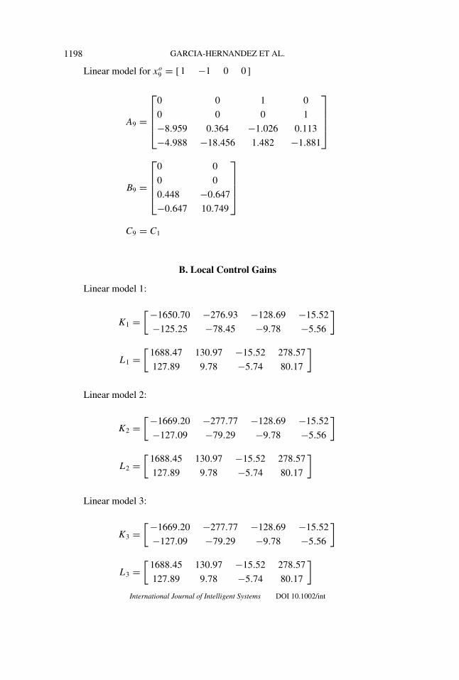
1198 GARCIA-HERNANDEZ ET AL.
Linear model for xo9 = [ 1 −1 0 0 ]
A9 =
⎡⎢⎢⎢⎣
0 0 1 0
0 0 0 1
−8.959 0.364 −1.026 0.113
−4.988 −18.456 1.482 −1.881
⎤⎥⎥⎥⎦
B9 =
⎡⎢⎢⎢⎣
0 0
0 0
0.448 −0.647
−0.647 10.749
⎤⎥⎥⎥⎦
C9 = C1
B. Local Control Gains
Linear model 1:
K1 =[−1650.70 −276.93 −128.69 −15.52
−125.25 −78.45 −9.78 −5.56
]
L1 =[
1688.47 130.97 −15.52 278.57
127.89 9.78 −5.74 80.17
]
Linear model 2:
K2 =[−1669.20 −277.77 −128.69 −15.52
−127.09 −79.29 −9.78 −5.56
]
L2 =[
1688.45 130.97 −15.52 278.57
127.89 9.78 −5.74 80.17
]
Linear model 3:
K3 =[−1669.20 −277.77 −128.69 −15.52
−127.09 −79.29 −9.78 −5.56
]
L3 =[
1688.45 130.97 −15.52 278.57
127.89 9.78 −5.74 80.17
]
International Journal of Intelligent Systems DOI 10.1002/int
REAL-TIME TAKAGI–SUGENO FUZZY CONTROL OF A ROBOT MANIPULATOR 1199
Linear model 4:
K4 =[−1593.90 −246.74 −124.46 −13.33
−101.02 −77.10 −7.77 −5.48
]
L4 =[
1630.91 126.74 −13.33 247.58
101.86 7.77 −5.65 77.99
]
Linear model 5:
K5 =[−1610.70 −245.90 −124.46 −13.33
−100.18 −76.26 −7.77 −5.48
]
L5 =[
1630.87 126.74 −13.33 247.57
101.85 7.77 −5.65 77.99
]
Linear model 6:
K6 =[−1613.30 −248.49 −124.46 −13.33
−102.76 −78.85 −7.77 −5.48
]
L6 =[
1630.88 126.74 −13.33 247.58
101.85 7.77 −5.65 77.99
]
Linear model 7:
K7 =[−1593.90 −246.74 −124.46 −13.33
−101.02 −77.10 −7.77 −5.48
]
L7 =[
1630.91 126.74 −13.33 247.58
101.86 7.77 −5.65 77.99
]
Linear model 8:
K8 =[−1613.30 −248.49 −124.46 −13.33
−102.76 −78.85 −7.77 −5.48
]
L8 =[
1630.88 126.74 −13.33 247.58
101.85 7.77 −5.65 77.99
]
Linear model 9:
K9 =[−1610.70 −245.90 −124.46 −13.33
−100.18 −76.26 −7.77 −5.48
]
International Journal of Intelligent Systems DOI 10.1002/int
1200 GARCIA-HERNANDEZ ET AL.
L9 =[
1630.87 126.74 −13.33 247.57
101.85 7.77 −5.65 77.99
]
C. � and � Matrices
Solving the linear matrix Equation 3, we obtain linear models from 1 to 9operation points:
�1 · · ·�9 =
⎡⎢⎢⎢⎣
1 0 0 0
0 0 0 1
0 1 0 0
0 0 −1 0
⎤⎥⎥⎥⎦
Linear model 1:
�1 =[
37.77304 2.28797 0.000007 1.64114
1.64118 −0.000006 −0.17499 1.72502
]
Linear model 2:
�2 =[
19.25485 2.28797 0.000007 0.80145
0.80157 −0.000006 −0.17499 0.88531
]
Linear model 3:
�3 =[
19.25485 2.28797 0.000007 0.80145
0.80157 −0.000006 −0.17499 0.88531
]
Linear model 4:
�4 =[
37.01204 2.28809 −0.000005 0.84015
0.84023 −0.000003 −0.17500 0.88543
]
Linear model 5:
�5 =[
20.17141 2.28809 −0.000005 1.67999
1.67989 0.000003 −0.17500 1.72522
]
Linear model 6:
�6 =[
17.58425 2.28809 −0.000005 −0.90720
−0.90718 0.000003 −0.17500 −0.86190
]
International Journal of Intelligent Systems DOI 10.1002/int
REAL-TIME TAKAGI–SUGENO FUZZY CONTROL OF A ROBOT MANIPULATOR 1201
Linear model 7:
�7 =[
37.01204 2.28809 −0.000005 0.84015
0.84023 −0.000003 −0.17500 0.88543
]
Linear model 8:
�8 =[
17.58425 2.28809 −0.000005 −0.90720
−0.90718 0.000003 −0.17500 −0.86190
]
Linear model 9:
�9 =[
20.17141 2.28809 −0.000005 1.67999
1.67989 0.000003 −0.17500 1.72522
]
International Journal of Intelligent Systems DOI 10.1002/int
Related Documents