Real time signals and data simulations for bionic hand ...

WARSAW UNIVERSITY OF TECHNOLOGY

Real time signals and data simulations

for bionic hand kinematics

by

Ferran Olid DominguezErasmus exchange student from

Polytechnic University of Catalonia

Barcelona School of Informatics

supervised by

Zbigniew Wawrzyniak Ph.D

A final bachelor project thesis

in the

Faculty of electronics and information technology

June 2016

Declaration of Authorship

I, Ferran Olid Dominguez, declare that this thesis titled, ‘Real time signals and data

simulationsfor bionic hand kinematics’ and the work presented in it are my own. I

confirm that:

� This work was done wholly or mainly while in candidature for a research degree

at this University.

� Where any part of this thesis has previously been submitted for a degree or any

other qualification at this University or any other institution, this has been clearly

stated.

� Where I have consulted the published work of others, this is always clearly at-

tributed.

� Where I have quoted from the work of others, the source is always given. With

the exception of such quotations, this thesis is entirely my own work.

� I have acknowledged all main sources of help.

� Where the thesis is based on work done by myself jointly with others, I have made

clear exactly what was done by others and what I have contributed myself.

Signed:

Date:

iii

“People always fear change. People feared electricity when it was invented, didnt they?

People feared coal, they feared gas-powered engines. There will always be ignorance, and

ignorance leads to fear. But with time, people will come to accept their silicon masters.”

Bill Gates

WARSAW UNIVERSITY OF TECHNOLOGY

Abstract

Faculty of electronics and information technology

by Ferran Olid Dominguez

Prosthesis have always been a necessity for the human being. In this thesis, EMG signals

are being collected, analyzed and processed in order to implement a real time algorithm

capable to differentiate two different states of a bionic hand. This document explains

how to obtain an algorithm with almost no false positives, and pretends to explain

why after this work, I can say that working with EMG signals is something way more

complicated that what someone could think.

Acknowledgements

It is a fact that a work is usually attributed to the one who develops and write a research

thesis, project or document. But truth is far away from this. If it would not be for the

help and knowledge that some people brought to this project, it would not be what it

is know.

These people supported, helped and understood me during the development of this

project in such a way I could not forget.

First I would like to thank my supervisor, director, and at the same way my tutor for this

thesis, Dr. inz Zbigniew Wawrzyniak, who was not only a work guide and helper, but

also an adviser during my stance in Poland. Not only did he helped me with the thesis,

but also encouraged me to present it to the ”XXXVIII-th IEEE-SPIE Joint Symposium

on Photonics, Web engineering, Electronics for Astronomy, and High Energy Physics

Experiments” conference.

I have also the need to thanks Richard Gomolka, Ph.D candidate who without any

further intention but interest in research and good will, helped me at many complicated

moments of this project, not only during the development of the code, but also during

the signal collection session. If that was not enough, he was also a friend during my

time in Warsaw, and helped me in so many ways I will never forget.

A person who also must be thanked is Dr. inz Ewa Piatkowska-Janko, who dedicated her

time to help me with the signal readings, and allowed me to use a brand new equipment

to carry out the data collection.

Finally, but not least, I want to give my most sincere thankfulness to all the Erasmus

students who made me feel like home during the development of this project, even being

kilometers away from it. Their cheers and way to be helped me to continue with this

thesis in the most difficult moments one can experience being far away from those who

love.

vi

Contents

Declaration of Authorship iii

Abstract v

Acknowledgements vi

List of Figures xi

List of Tables xiii

Abbreviations xv

I Project management 1

1 Context 3

1.1 Introduction . . . . . . . . . . . . . . . . . . . . . . . . . . . . . . . . . . . 3

1.2 Reading the mind . . . . . . . . . . . . . . . . . . . . . . . . . . . . . . . . 3

1.3 Actors involved . . . . . . . . . . . . . . . . . . . . . . . . . . . . . . . . . 4

1.3.1 Developer . . . . . . . . . . . . . . . . . . . . . . . . . . . . . . . . 4

1.3.2 Director and support . . . . . . . . . . . . . . . . . . . . . . . . . . 4

1.3.3 Beneficiaries . . . . . . . . . . . . . . . . . . . . . . . . . . . . . . . 4

2 State of the art 5

2.1 Actual state . . . . . . . . . . . . . . . . . . . . . . . . . . . . . . . . . . . 5

2.1.1 Muscle signals . . . . . . . . . . . . . . . . . . . . . . . . . . . . . 5

2.1.2 Nerve signals . . . . . . . . . . . . . . . . . . . . . . . . . . . . . . 6

2.2 Scope of the project based on the state of the art . . . . . . . . . . . . . . 6

3 Scope of the project 9

3.1 Main goal . . . . . . . . . . . . . . . . . . . . . . . . . . . . . . . . . . . . 9

3.2 Stages . . . . . . . . . . . . . . . . . . . . . . . . . . . . . . . . . . . . . . 9

3.3 Risks . . . . . . . . . . . . . . . . . . . . . . . . . . . . . . . . . . . . . . . 10

3.3.1 Not having access to the signal recording laboratory . . . . . . . . 10

3.3.2 Delay in implementation time . . . . . . . . . . . . . . . . . . . . . 10

vii

viii CONTENTS

4 Temporal plannification 11

4.1 Task definition . . . . . . . . . . . . . . . . . . . . . . . . . . . . . . . . . 11

4.1.1 Project management . . . . . . . . . . . . . . . . . . . . . . . . . . 11

4.1.2 Movement definition . . . . . . . . . . . . . . . . . . . . . . . . . . 12

4.1.3 Signal reading . . . . . . . . . . . . . . . . . . . . . . . . . . . . . 12

4.1.4 Study the state of the art . . . . . . . . . . . . . . . . . . . . . . . 12

4.1.5 Obtained signal processing . . . . . . . . . . . . . . . . . . . . . . 13

4.1.5.1 Determinate the algorithm to use . . . . . . . . . . . . . 13

4.1.5.2 Implementation . . . . . . . . . . . . . . . . . . . . . . . 13

4.1.5.3 Analysis, interpretation and evaluation of results . . . . . 13

4.1.6 Software-hardware bridge . . . . . . . . . . . . . . . . . . . . . . . 14

4.1.7 Real time simulation . . . . . . . . . . . . . . . . . . . . . . . . . . 14

4.1.8 Final stage . . . . . . . . . . . . . . . . . . . . . . . . . . . . . . . 14

4.2 Time estimation per task . . . . . . . . . . . . . . . . . . . . . . . . . . . 14

4.3 Task dependencies . . . . . . . . . . . . . . . . . . . . . . . . . . . . . . . 14

4.4 Gantt diagram . . . . . . . . . . . . . . . . . . . . . . . . . . . . . . . . . 15

5 Resources 17

5.1 Human resources . . . . . . . . . . . . . . . . . . . . . . . . . . . . . . . . 17

5.2 Software resources . . . . . . . . . . . . . . . . . . . . . . . . . . . . . . . 17

5.3 Hardware resources . . . . . . . . . . . . . . . . . . . . . . . . . . . . . . . 18

6 Deviation and acting plan 19

7 Economic management 21

7.1 Budget . . . . . . . . . . . . . . . . . . . . . . . . . . . . . . . . . . . . . . 21

7.2 Management Control . . . . . . . . . . . . . . . . . . . . . . . . . . . . . . 22

8 Sustainability and social commitment 23

8.1 Economic scope . . . . . . . . . . . . . . . . . . . . . . . . . . . . . . . . . 23

8.2 Social scope . . . . . . . . . . . . . . . . . . . . . . . . . . . . . . . . . . . 24

8.3 Environmental scope . . . . . . . . . . . . . . . . . . . . . . . . . . . . . . 24

II Development 25

9 Movement definition and signal readings 27

9.1 EMG signals and Lab equipment . . . . . . . . . . . . . . . . . . . . . . . 27

9.1.1 EMG signals . . . . . . . . . . . . . . . . . . . . . . . . . . . . . . 27

9.1.2 Lab Equipment . . . . . . . . . . . . . . . . . . . . . . . . . . . . . 28

9.2 EMG signal readings . . . . . . . . . . . . . . . . . . . . . . . . . . . . . . 28

9.2.1 First session: constant rhythm finger flexions . . . . . . . . . . . . 29

9.2.2 Second session: whole fist contraction . . . . . . . . . . . . . . . . 30

9.2.3 Third session: RT dataset . . . . . . . . . . . . . . . . . . . . . . . 32

10 Processing and filtration of the obtained signals 33

10.1 First session - dealing with poor signals . . . . . . . . . . . . . . . . . . . 33

10.1.1 First filters and envelope . . . . . . . . . . . . . . . . . . . . . . . 34

CONTENTS ix

10.1.2 Adjusting the frequency spectrum . . . . . . . . . . . . . . . . . . 36

10.1.2.1 Adjusting Notch filter . . . . . . . . . . . . . . . . . . . . 37

10.2 Second session - stronger, longer signals . . . . . . . . . . . . . . . . . . . 39

11 Designing the real time algorithm 43

11.1 Introduction to Real Time processing . . . . . . . . . . . . . . . . . . . . . 43

11.2 Algorithm requirements and characteristics . . . . . . . . . . . . . . . . . 44

11.2.1 Filters selection . . . . . . . . . . . . . . . . . . . . . . . . . . . . . 45

11.2.2 Structure of the algorithm . . . . . . . . . . . . . . . . . . . . . . . 46

11.3 Algorithm detailed explanation . . . . . . . . . . . . . . . . . . . . . . . . 48

11.3.1 Calibration - emg calibrate.m . . . . . . . . . . . . . . . . . . . . 48

11.3.2 Processing chunks - filter chunk.m . . . . . . . . . . . . . . . . . 49

11.3.3 Taking decisions - check active.m . . . . . . . . . . . . . . . . . . 49

11.4 Other aspects of the algorithm . . . . . . . . . . . . . . . . . . . . . . . . 52

III Results, conclusions and future work 53

12 Results and conclusions 55

12.1 Results . . . . . . . . . . . . . . . . . . . . . . . . . . . . . . . . . . . . . . 55

12.1.1 About EMG . . . . . . . . . . . . . . . . . . . . . . . . . . . . . . 55

12.1.2 About the RT algorithm . . . . . . . . . . . . . . . . . . . . . . . . 56

12.2 Conclusions . . . . . . . . . . . . . . . . . . . . . . . . . . . . . . . . . . . 57

12.2.1 Conclusions about EMG signals . . . . . . . . . . . . . . . . . . . . 57

12.2.2 Conclusions about the algorithm . . . . . . . . . . . . . . . . . . . 58

12.3 Future work . . . . . . . . . . . . . . . . . . . . . . . . . . . . . . . . . . . 58

A Extra figures 61

A.1 Project budget . . . . . . . . . . . . . . . . . . . . . . . . . . . . . . . . . 61

A.2 Lab equipment . . . . . . . . . . . . . . . . . . . . . . . . . . . . . . . . . 62

B Matlab code 63

B.1 EMG quick processing function - emg qp.m . . . . . . . . . . . . . . . . . 63

B.2 Algorithm main body - ttest RT EMG processing.m . . . . . . . . . . . . 67

B.3 Reading signals - read signals.m . . . . . . . . . . . . . . . . . . . . . . . . 70

B.4 Calibration function - emg calibrate.m . . . . . . . . . . . . . . . . . . . . 70

B.5 Processing chunk - filter chunk.m . . . . . . . . . . . . . . . . . . . . . . . 71

B.6 Value updater - update values.m . . . . . . . . . . . . . . . . . . . . . . . 72

B.7 Deciding function - ttest check active.m . . . . . . . . . . . . . . . . . . . 73

B.8 Normalize cycles - normalize cycles.m . . . . . . . . . . . . . . . . . . . . 74

B.9 Repository . . . . . . . . . . . . . . . . . . . . . . . . . . . . . . . . . . . . 75

Bibliography 77

List of Figures

2.1 EMG electrode display . . . . . . . . . . . . . . . . . . . . . . . . . . . . . 6

4.1 Gantt diagram . . . . . . . . . . . . . . . . . . . . . . . . . . . . . . . . . 15

9.1 Electrode spots for first session . . . . . . . . . . . . . . . . . . . . . . . . 29

9.2 Electrodes spots for second session . . . . . . . . . . . . . . . . . . . . . . 30

10.1 Raw signal for middle finger flexion . . . . . . . . . . . . . . . . . . . . . . 34

10.2 Before Notch filter . . . . . . . . . . . . . . . . . . . . . . . . . . . . . . . 35

10.3 After Notch filter . . . . . . . . . . . . . . . . . . . . . . . . . . . . . . . . 35

10.4 RMS basic formula . . . . . . . . . . . . . . . . . . . . . . . . . . . . . . . 35

10.5 Raw signal, RMS filtered signal, and superposition of both . . . . . . . . . 36

10.6 α = 0.5 . . . . . . . . . . . . . . . . . . . . . . . . . . . . . . . . . . . . . 38

10.7 α = 0.2 . . . . . . . . . . . . . . . . . . . . . . . . . . . . . . . . . . . . . 38

10.8 α = 0.05 . . . . . . . . . . . . . . . . . . . . . . . . . . . . . . . . . . . . . 38

10.9 α = 0.005 . . . . . . . . . . . . . . . . . . . . . . . . . . . . . . . . . . . . 38

10.10emg qp flowchart . . . . . . . . . . . . . . . . . . . . . . . . . . . . . . . . 39

10.11signal 1 (contractors) raw . . . . . . . . . . . . . . . . . . . . . . . . . . . 39

10.12Signal after high pass and low pass filters . . . . . . . . . . . . . . . . . . 40

10.13Signal after application of Notch filter . . . . . . . . . . . . . . . . . . . . 41

10.14Signal after moving averaging . . . . . . . . . . . . . . . . . . . . . . . . . 42

11.1 Algorithm diagram . . . . . . . . . . . . . . . . . . . . . . . . . . . . . . . 47

11.2 Weights applied in the mean . . . . . . . . . . . . . . . . . . . . . . . . . 50

12.1 Signal interpreted by the algorithm . . . . . . . . . . . . . . . . . . . . . . 56

A.1 NI ELVIS II . . . . . . . . . . . . . . . . . . . . . . . . . . . . . . . . . . . 62

A.2 EKG sensor . . . . . . . . . . . . . . . . . . . . . . . . . . . . . . . . . . . 62

A.3 Dynamometer . . . . . . . . . . . . . . . . . . . . . . . . . . . . . . . . . . 62

xi

List of Tables

4.1 Time estimation per task . . . . . . . . . . . . . . . . . . . . . . . . . . . 15

4.2 Task dependencies . . . . . . . . . . . . . . . . . . . . . . . . . . . . . . . 15

11.1 Filters applied in the real time algorithm . . . . . . . . . . . . . . . . . . 46

xiii

Abbreviations

EMG ElectroMyoGram

RMS Root Mean Square

RT Real Time

xv

Dedicated to every single teacher, person or life being that helpedme to get where I am. Thank you for making me who I am now;

this is for you all.

xvii

Part I

Project management

1

Chapter 1

Context

1.1 Introduction

In the world we are living, there is a great number of human injuries which end up

with the amputation of an extremity. During the history, there has been created several

types of prosthesis that allowed people to, somehow, carry on with their daily life. These

prostheses have gone from simple wooden legs to first attempts of bionic hands.

These last prosthesis, bionics, are allowed to interpret the thinking of the patient in

order to represent these thoughts into a movement like done with the human biologic

extremity.

The main target of this project is to achieve the simulation of a bionic hand that is

capable to work in real time. This is, obtaining real data experimentally from a forearm

and decide the kinematics of a robotic hand according to the characteristics of these

signals.

1.2 Reading the mind

Saying that a robotic arm is capable of construing the mind of a person and represent

it seems something related to neuroscience and medicine, and that, in order to achieve

such a thing, brain scans would be needed. Nevertheless, reality is far away from that.

Bionic prosthesis construe the signal from the brain, that is true, but they do not analyze

directly this organ, but the signals spread from it along communication channels: nerves

and muscles.

3

4 Chapter 1 Context

Then as mentioned, these prostheses read the electrical signals from nerves and muscles,

construe them using machine learning algorithms and artificial neuronal networks to

finally reproduce the desired movement into the robotic arm or hand.

It is important to remark that there is a difference of functions between the two signals.

Nerves are in charge of control and response of the hand, while muscles are the direct

effectors from these nerve signals in charge of creating the mechanical effect which is the

movement of the hand.

1.3 Actors involved

During the development of this project there is a set of people involved in it, either

directly or indirectly. We describe these people in the following lines.

1.3.1 Developer

The developer is the person in charge of carry out the project. This is the most involved

and implicated person in the project, since is the person in charge of the planification

and development of the project, as well as the one defending the project in the oral

presentation and the writer of the memory. It is responsible for delivering and finish all

the task on time or carry out the actuation plan of necessary.

1.3.2 Director and support

The director is the person in charge of the developer. His duty is to, using its expertise

in the field, lead the developer and help him to take the right decisions. Some other

important people in the development of the project are two researches from the university

of Warsaw, who will help on obtaining the signals and the signal processing of the signals.

These persons are Dr. in Ewa Piatkowska-Janko and PhD candidate Richard Gomolka.

1.3.3 Beneficiaries

In the case of this project there are two types of beneficiaries. The first one is really

clear: amputees, which will have better products to continue their life in a more regular

way. The other group of people who can benefit from this project is everyone in the

scientific field, since this project can be used for further investigation along with the

collected data.

Chapter 2

State of the art

2.1 Actual state

Actually this field is found under development. There are already some prosthesis ca-

pable of interpret basic movements, but these movements are slow in addition of being

very limited.

We can say hence, that is a sector which is in a very primitive state having in mind

what it wants to achieve (real movement of a human hand). Nowadays, the target of

the research are the algorithms and methods of signal processing which have to be used

for the right detection and filtering of the nerve in EMG signals[1], [2], [3], [4], [5], .

If we take a look at the most interesting results, we can appreciate how the decoding of

the signals can achieve to move some fingers separately[6].

In addition, the ideal would be to achieve that these kinds of prostheses have an afford-

able price for the middle class, since the mean price for these prosthesis is around 10,000

euros.

Another remarkable thing to talk about in this section is the hardware used to read

these signals from the body. There are actually two sources of information for bionic

purposes: muscles and nerves.

2.1.1 Muscle signals

The first one seems a little weird since we are talking about amputees, but however,

muscles from the forearm react in different ways against different hand movements, so

we can take advantage of the electrical signals from these muscles to reproduce the

5

6 Chapter 2 State of the art

movement, a.k.a, EMG signals. The actual greatest problem with this kind of signals is

the noise recorded also in the signal.

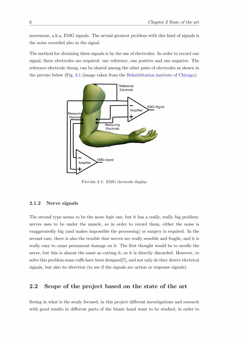
The method for obtaining these signals is by the use of electrodes. In order to record one

signal, three electrodes are required: one reference, one positive and one negative. The

reference electrode thoug, can be shared among the other pairs of electrodes as shown in

the picture below (Fig. 2.1 (image taken from the Rehabilitation institute of Chicago):

Figure 2.1: EMG electrode display

2.1.2 Nerve signals

The second type seems to be the more legit one, but it has a really, really big problem:

nerves uses to be under the muscle, so in order to record them, either the noise is

exaggeratedly big (and makes impossible the processing) or surgery is required. In the

second case, there is also the trouble that nerves are really sensible and fragile, and it is

really easy to cause permanent damage on it. The first thought would be to needle the

nerve, but this is almost the same as cutting it, so it is directly discarded. However, to

solve this problem some cuffs have been designed[7], and not only do they detect electrical

signals, but also its direction (to see if the signals are action or response signals).

2.2 Scope of the project based on the state of the art

Seeing in what is the study focused, in this project different investigations and research

with good results in different parts of the bionic hand want to be studied, in order to

Chapter 2 State of the art 7

merge them and achieve very efficient results.

Designing a new data obtaining system or a new signal processing algorithm would be

really expensive, either in the economic field as in time. This is like this since the

actual algorithms are researches carried out by professional research teams in periods

of years. Moreover, digital signal processing knowledges which are not obtained during

the computer engineering degree are required.

In the economic field, the university does not have enough resources to afford the costs,

even less for an exchange student. However, some materials to read biological signals

can be obtained.

Chapter 3

Scope of the project

3.1 Main goal

The main goal of the project is to design a software capable of process signals from the

forearm and classify them into different movements of a real hand, and then translate

this classifications into robotic hand kinematics.

As mentioned during the document, during the development of this project, several

methods of signal processing for EMG signals in the field of bionic hand will be studied.

Then, based on theses studies, the algorithm will be implemented, merging all the good

results from these previous studies in order to achieve an optimal result.

Afterwards, the kinematics for the robotic hand will be correlated to the algorithm

output and finally, a real time simulation is going to take place.

3.2 Stages

1. During the first stage of the project, current algorithms are going to be studied,

and a selection of the best will be made.

2. Next, basic movements of the hand will be defined to read as EMG signals to have

a database to work with. Basic movements will be wanted, which together, can

cover most of the main movements of a hand.

3. Once the movements are defined, the reading of these movements using electrodes

will be registered to obtain EMG signals.

9

10 Chapter 3 Scope of the project

4. When the database is obtained, the signals will be processed and filtered, so after-

wards we can classify the different types of signals into different movements using

a classification algorithm.

5. With the classification algorithm giving good results, the kinematics of the hand

can be implemented, and hence do the real time simulation can take place.

3.3 Risks

During the development of the project, there can be some things not going according to

the plan. If these situation occurred, here we present some alternatives:

3.3.1 Not having access to the signal recording laboratory

There is no access to the laboratory to record signals from the forearm.

Solution: We would use some set of data provided by other papers on the matter. To

do the real time simulation, we would use some of these data as training data for the

algorithm, and some other as simulated real time data.

3.3.2 Delay in implementation time

The signal processing, filtering and classification takes longer than expected

Solution: We would invest more hours per day. If this would not be enough we would

end up using a simpler algorithm with less cases to classify.

Chapter 4

Temporal plannification

The development time for this project is around 5 months: from March until July, both

from year 2016. In the following pages, the planification of this project is explained,

bearing in mind flexibility, unexpected events and incidents.

In order to solve these kind of delays, actuation plans are presented.

4.1 Task definition

In this section of the document, as its name indicates, the different tasks of the project

are defined and explained.

4.1.1 Project management

In this section of the project which is carried out in the subject GEP from FIB, the time

and tasks of the project are defined, as well as the budget and the impact of it. The

subject has a total of 7 subtasks to deliver:

• Scope of the project

• Temporal planification

• Economic management and sustainability

• Preliminary presentation

• Contextualization and bibliography

• Specification

11

12 Chapter 4 Temporal plannification

• Oral presentation and final document

As indicated in the subject definition, the estimated time for this task is 75 hours.

4.1.2 Movement definition

Before reading the EMG signals in order to relate them to mechanical movements of

a robotic arm, we must find a set of movements of interest. To do that, a set of

basic movements will be defined, this is: movements that together shape the totality of

movements of the hand.

Some more complex movements will be recorded as well to see how the algorithm deals

with these kind of movements apart of the previously defined basic ones.

To do this, we will work with people with bionic and biological signal reading experience.

For this task, a time of 15 hours is expected.

4.1.3 Signal reading

In this task, the EMG signals of the arm will be read. If possible, from different people.

The EMG signals are electrical signals generated by the activity of the muscle. This

signals will be recorded using a set of electrodes which can be sticked on the skin.

Since the lectures take some sessions to be recorded (sometimes there are problems with

the equipment or the noise in the signals is too high) 30 hours will be taken for this

task.

4.1.4 Study the state of the art

Since the bionic matter is completely under development, the observation of the different

techniques used to decipher the signals with best results until the moment is required,

as well as find which are the most important muscles to record, data structures used

and more previous knowledges which are not obtained during the degree.

Even being still under development, several information and documents can be found

about bionic and biological signal processing, hence the estimated time for this task is

50 hours.

Chapter 4 Temporal plannification 13

4.1.5 Obtained signal processing

This task is the most important on the project. In the existing documentation about

bionics, they continuously talk about the filtering and processing of the signal as men-

tioned before.

During this stage, which has a length of 340 hours, the following subtasks are defined:

4.1.5.1 Determinate the algorithm to use

During this subtask, the different algorithms and data structures explained in the sci-

entific papers studied in the previous task will be evaluated and selected.

From all these algorithms, we will study which are the most efficient and which are more

useful for our project bearing in mind the time and knowledges that we have. It has to

be considered that the final product should work in real time.

This stage is crucial for the project, from it depends the performance of the final product.

Therefore, 80 hours will be dedicated on it.

4.1.5.2 Implementation

This is the longest subtask of the project, in which the software in charge of interpret

and classify the signals will be developed according to the algorithms and data structures

selected in the previous subtask.

Since we know from experience that the implementation of a software is very time

expensive, a total amount of 160 hours will be assigned to this stage.

4.1.5.3 Analysis, interpretation and evaluation of results

Once the required software has been implemented, the results obtained from it will be

analyzed.

In order to evaluate the efficiency of the algorithm, the following requisites will be

considered:

• Processing time

• Clearness of processed signals

14 Chapter 4 Temporal plannification

• Amount of hit and miss when interpreting signals

• Possible hardware optimization of the code

The first one indicates the speed in which the algorithm can process the signals. The

second one will tell us the quality of the filtering and processing on the signal. The third

is probably the most important one, telling us how many times the algorithm worked

well or bad. Finally in the last section, we will evaluate which is the portability of the

code into some hardware platform with the ability to optimize code via hardware, such

as FPGA, Arduino or other embedded systems.The time for this subtask is 100 hours.

4.1.6 Software-hardware bridge

During this stage of the project the kinematics of a bionic hand will be implemented

from the results of the previous task. A total of 20 hours will be invested.

4.1.7 Real time simulation

Finally, and if the equipment is available from the medical university, some real time

tests will be done on the algorithm. This way we will be able to evaluate if the project

achieves the main target of interpreting and classify signals in real time. 20 hours will

be dedicated to this task.

4.1.8 Final stage

During this stage the memory of the project will be redacted as well as the possible

paper for it. Also, the defense of the presentation will held. The estimated time is

50 hours for this task.

4.2 Time estimation per task

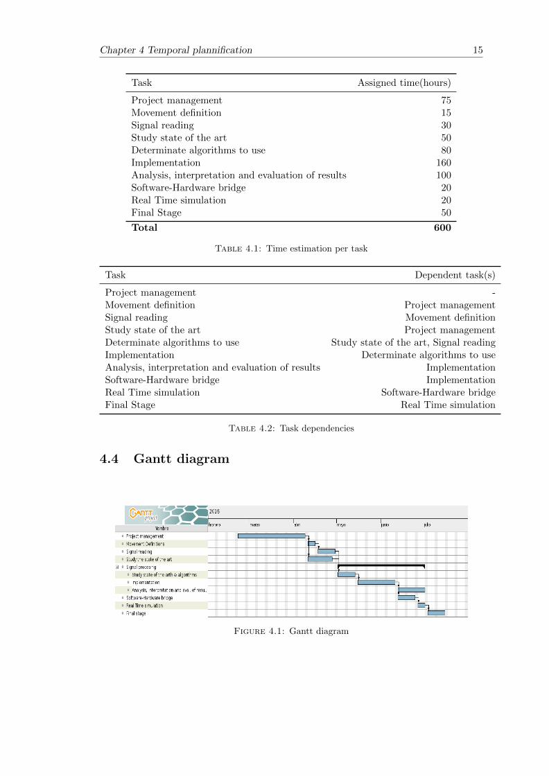
In the following table, a summary of the assigned hours is shown:

4.3 Task dependencies

Chapter 4 Temporal plannification 15

Task Assigned time(hours)

Project management 75Movement definition 15Signal reading 30Study state of the art 50Determinate algorithms to use 80Implementation 160Analysis, interpretation and evaluation of results 100Software-Hardware bridge 20Real Time simulation 20Final Stage 50

Total 600

Table 4.1: Time estimation per task

Task Dependent task(s)

Project management -Movement definition Project managementSignal reading Movement definitionStudy state of the art Project managementDeterminate algorithms to use Study state of the art, Signal readingImplementation Determinate algorithms to useAnalysis, interpretation and evaluation of results ImplementationSoftware-Hardware bridge ImplementationReal Time simulation Software-Hardware bridgeFinal Stage Real Time simulation

Table 4.2: Task dependencies

4.4 Gantt diagram

Figure 4.1: Gantt diagram

Chapter 5

Resources

During the development of this project different types of resources are going to be used.

Among them we can find human, software and hardware resources, which will all be

described below.

5.1 Human resources

This project will be developed by a student in computer science, specialized in the matter

of computer engineering. Moreover, a couple of experts in electromyogram and medicine

will also temporarily collaborate in the obtainment of the signals needed in the project.

5.2 Software resources

During the development of the project we will mainly work with the tool Matlab for the

treatment and study of the signals. Anyway, the following tools shall also be used:

• Google Drive: online platform for data storage and office documents creation and

edition.

• Texmaker: LaTeX text compiler and editor

• Atenea: Learning platform

• Adobe Reader and Okular: PDF file viewer

• FIBs Rac: Tool for the academic management and virtual campus.

• GanttProject: Tool to generate Gantt diagrams

17

18 Chapter 5 Resources

• LibreOffice: Set of programs for office documents

5.3 Hardware resources

The expected hardware resource in this project are rather low. Since the project consist

mainly on signal study and processing, only the following materials are going to be used:

• Personal computer: ASUS GL552JX-XO265 along with a Logitech G5 mouse.

• Electrodes: for the electromyogram and nerve signal reading.

Chapter 6

Deviation and acting plan

In this kind of project it is very common for deviations to happen on the original plan,

since it is very hard to know for sure the time which is going to be spent in every task

before the project starts. However we are applying a Scrum methodology, which allows

us to control in some way the possible deviations. These are the steps to follow in case

of a deviation:

• textbfIn case a task ends before expected: the next task is started without problem.

• textbfIn case a task ends after expected: If the delay is not much, the task is

finished and the next one is started. Nevertheless if the delay is too big the tasks

Implementation, Result analysis and Real time simulation will be prioritized. If

some of these prioritized stages takes way longer than expected, we will focus on

implementation and result analysis.

These deviations could affect a little bit on hardware resources, especially in the use of

the personal computer. However the difference in the budget would be minimum (less

than 1), so we can depreciate it. We can say that this planification guarantees the end

of the project by the assigned date.

19

Chapter 7

Economic management

7.1 Budget

As shown in the table found in the appendix, section Project budget, the budget for

the project has been estimated taking the resources specified before and using the plan-

ification explained in the previous section. In the making of this table, either hardware

and software resources, as well as human resources have been beared in mind. In some

tasks, incidentals have been also considered, and so has been the contingency.As seen in

the table, first of all direct costs for every task are specified for hardware, software and

human resources.

For those hardware and software which will be further used out of the project because

of its use life, a proportion has been applied over the total price in order to calculate

which part of its life will be used. Regarding those software resources which prices are

not specified or are either 0, this is because those softwares are Free Software, and hence

the price for them is 0.

As for what human resources concerns and as mentioned before, there is just one student

of computer engineering working on the project, but at a given point there will be a

collaboration from two experts in the matter who will help on the setting up of the

electrodes for free.

Indirect costs (in this case electricity for working during no-light hours and Internet)

are applied. Luckily in Poland these costs are rather low as shown in the budget.

Moreover incidentals are also considered. These costs have been applied only on those

tasks where there is a real risk of exceeding the planified resources, this is, on signal

reading, state of the art study, implementation, results analysis and final stage.

21

22 Chapter 7 Economic management

Finally a low contingency (3%) and VAT (21%) are applied on the total cost.

7.2 Management Control

During the development of the project some deviations may occur, causing some tasks

to take longer than expected. These deviations can be rectified with with an action plan.

However, we need to establish some way to calculate these deviations over the initial

budget.

We did not applied deviations to all the tasks, only to those we think that have a real risk

to suffer some unexpected incident. These tasks are the following: signal reading, state

of the art studying, implementation, result analysis and final stage. After the project

has been carried out, the real working time of these stages will be compared with the

theoretical time specified in this document. If the difference is huge, the reason why this

happened will be studied and hence avoided in future works.

Finally, since the project is rather short and the tasks have been well specified, a very

low contingency of 3% has been applied on the budget.

Chapter 8

Sustainability and social

commitment

In order to make a study of the sustainability of the project along with the social

commitment, three different scopes are going to be considered: economic, social and

environmental. In order to rate these aspects, we are going to answer some question and

base the final score on these answers.

8.1 Economic scope

In the economic scope, this project has a mark of 9.2. The reasons for this mark are the

following:

• The cost of the project is really studied for every kind of resource;

• It is just a scientific study, and hence it does not require any kind of maintenance;

• It is a very cheap project, so it would be really good if launched in the market;

• The project pretends to create a solution for the arm movements of a bionic hand,

so it presents a solution in the market.

• If carried out by a more experimented engineer, the development time would be

less.

23

24 Chapter 8 Sustainability and social commitment

8.2 Social scope

In the social scope, this project has a mark of 9.5. Here there are the reasons why it

obtained this mark:

• Personally, the project provides me of a set of new knowledges which will help me

in my future working live

• The target of the project (disabled people with an amputated hand) will benefit

from this project by having access to cheaper bionic prosthesis.

• There are no third parties in which this project affects on a negative way.

• This project has been presented to solve a problem in the society.

8.3 Environmental scope

In the environmental scope, this project has a mark of 8.2. Below are the reasons for

this mark.

• This project, by itself, has no impact on the environment, but only the electricity

used by the computer during the working hours;

• In the future, it is possible that this project is used for the mass productivity of

bionic arms, hence this mass production could have an impact on the environment;

• For the development of this project, several works can be used as a base for the

project;

• Most likely, the project will not produce any negative impact on environment;

• Most likely, the project can be reused for further work in the subject.

Part II

Development

25

Chapter 9

Movement definition and signal

readings

During the development of the project, different signal readings have been carried on.

Because of this, in every reading session we fixed mistakes committed in the previous

one; either right placement of the electrodes or wrong movements to record among

others. In the following sections within this chapter, we will describe which movements

where recorded in every session, as well as the usage done of the available material.

Furthermore, the mistakes and the impact of those in the readings, will be explained

and discussed. However, the detailed explanation of how these issues were solved will

be explained in the next chapter.

Therefore, in this chapter we will focus on the obtainment of the signals, the issues

this obtainment can generate and the solutions we have found.

9.1 EMG signals and Lab equipment

The first thing to know about the recording of our EMG signals is which equipment was

used and understanding how EMG recordings are made. In this section we will explain

with detail which equipment was disposed during the recordings, as well as how EMG

signals are recorded.

9.1.1 EMG signals

Before talking about how EMG signals are recorded, it is important to understand what

they are exactly. In a very simple way, we can refer to EMG samples as electrical

27

28 Chapter 9 Movement definition and signal readings

signals generated by muscles. However, what is really happening at a very low

physiological level is that every muscle cell has an ionic difference between its parts,

and, when this cell is excited, an electrical perturbation occurs. When this happens

with many muscle cells, an electrical signal is generated, and thus we can record it with

electrodes as detailed in the previous chapter (exposed in figure 2.1).

9.1.2 Lab Equipment

Now that we understand how EMG signals are recorded, we are ready to know which

equipment was used for our readings. In our case, we use a set of academic material

from National Instruments.In this set we can basically find the following devices:

• NI ELVIS II(User manual) Board capable of reading EMG (among others) signals

and transform them for further use in a computer

• EKG sensor 200: Captures signals from electrodes, amplifies them so afterwards

can be sended to the NI ELVIS II.

• Hand dynamometer: This device allows to record strength applied by the hand,

either from whole hand or the climp between two fingers.

Pictures of these equipment can be seen in the Appendix.

As for what the software refers, we have been usign a software designed by the same

company called LabView, which allows to take the channels from the NI Elvis II and

monitor them in real time. Moreover, with this software platform we could export the

data files in a Matlab format, in order to be processed and studied afterwards.

9.2 EMG signal readings

What we want to achieve by reading this kind of signal is a signal with which we can

easily or clearly decide the state of the hand. Thus, we aim to get some clear signals

with the minimum amount of noise.

Since we want to get information from the hand we want to measure the muscles in

charge of moving the fingers; this is, most of the muscles in the forearm. Therefore, let

us take a look at the different sessions that were carried out in order to get these data.

Chapter 9 Movement definition and signal readings 29

9.2.1 First session: constant rhythm finger flexions

This session was our first contact with the lab equipment and was the first time we

were facing an EMG recording. By then we thought that it would be a good idea to

record 10 flexions for every single finger, each flexion every one second. Also, the clamp

between the thumb with all the other fingers (one by one) was recorded. It is important

to remark that these flexions were mere impulses, this is, the flexion of the finger was

not kept for a whole second.

Figure 9.1: Electrode spots for first session

Regarding the number of electrodes and its position, we did the following deployment:

1. Reference electrode: placed in the middle of the forearm, serves as reference

for all the other electrodes.

2. Inner wrist tendons: Two electrodes were placed over the tendons in the wrist

in order to check the strength on the contraction of each finger. This movement

is caused by the contraction of both flexor carpum muscles.

3. upper-outer forearm: The other two electrodes where placed in the outer part

of the forearm, close to the elbow. With this, we can read the strength on the

extension of each finger, given by the activity by the smaller forearm extensors.

Regarding Figure 9.1, there are some things we have to remark. The first thing we must

notice is the different types of electrodes used during the recording. Also, it is important

to point out that the electrode close to the elbow, are not well stuck on the skin surface.

30 Chapter 9 Movement definition and signal readings

Furthermore, we used different types of electrodes, the wires were moving during the

recording and, as expectable, the movement of a finger causes a very small EMG reac-

tion from the muscle. Because of these issues among others, the first recording session

resulted in some poor signals. However, with these signals we could start to work on the

filtration and processing of the signals, as well as getting to know the main characteristics

of the EMG signals produced by our equipment.

9.2.2 Second session: whole fist contraction

As mentioned before, we could work somehow with the signals from the first session but

one of the main problems was that those were weak. We needed some sort of signal that

could be easily differentiated from the baseline (relaxed position of the arm). In addition,

we also noticed that there were no appreciable differences between the flexion of every

particular finger. For all these reasons we opted to register the whole fist contraction,

with full strength, for the next session.

Moreover we deemed that this time, instead of with impulses, we should work with some

sort of signal that kept the EMG signal activated for a while. This way we could be

able to study the nature of the EMG in a more accurate way, since the impulses were

not providing enough characteristics of the signals.

Therefore, for the second session of EMG recording, we read the EMG signals of the

forearm for fist contractions of 2 seconds, in intervals of 2 seconds. This means that

the whole cycle is around 4 seconds.

Figure 9.2: Electrodes spots for second session

Chapter 9 Movement definition and signal readings 31

The position of the electrodes, as shown in figure 9.2 vary a little from the previous

display. In this session we had:

1. Reference electrode: The reference electrode was this time placed a little closer

to the elbow than before. There is not a particular reason for it to be closer, but

the thing is that in this spot, there is no muscular activity during the recording,

and there are neither veins nor nerves that can cause noise. In figure 9.2, these

are the electrodes with a black pin.

2. Flexor carpi: Instead of the wrist tendons, which provide a very low EMG signal,

for this session we opted to locate the electrodes right on the muscles in charge of

the contraction of the four last fingers: the flexor carpi muscles. In figure 9.2 we

can identify these electrodes as the ones with the red pin.

3. Extensor carpi: These electrodes are located in the same place as in the previous

reading, right on the Extensor carpi muscle set, close to the elboy by the outter

part of the arm. Those are not very visible in figure 9.2, but we can see a part of

an electrode with a green pin.

We can also see in the picture that there is a dynamometer. It was used basically to

see the strength (in newtons) applied by the hand. The purpose of this signal was to

correlate somehow the power of the EMG with the strength delivered by the fist, but it

was not used in the end.

In this session, we obtained very pleasant signals. The noise was basically the same, but

this time the electrodes were well located and we avoided some noise generated by the

movement of the wires. In addition, since the movement recorded was the whole fist,

the power of the EMG when the muscles were active was way more powerful than the

power generated by the finger flexion, as we did in session one.

With these signals, we were able to find out the last characteristics we needed from the

EMG and start to design and test the RT-algorithm, which let’s not forget is the main

target of this project.

The only problem with the signals obtained was that they were too much periodic. With

these I mean that in a real case of a bionic arm, the movements are rather aperiodic,

so we needed some signals with different timings to test the RT-algorithm in a reliable

way.

32 Chapter 9 Movement definition and signal readings

9.2.3 Third session: RT dataset

This was the third and last session of EMG recording for this project. In this session we

also registered the whole fist flexion, but this time we used different timings. We had

a total of 3 dataset, both with 2 signals as in the previous sessions. The first dataset

contains different duration of contraction, but it could not be used due to some strange

really high noise that appeared during the session. The second and third dataset contain

contractions of 4 seconds, but with different level of strengths.

In this session there was no a very strict time synchronisation, but that was the intended

purpose of this session: to produce signals to test if the algorithm could detect the cycles

in which the muscle is activated.

The deployment of the electrodes was the same as in the previous session. However, this

time we glued the wires on the table in order to avoid wire noise, which seemed to be

the one causing the biggest distortion.

Chapter 10

Processing and filtration of the

obtained signals

Before talking about the filtration we applied on the obtained EMG signals, let us talk

a little bit about the nature of these signals.

In most of the cases, when we look at a raw EMG signal, we can appreciate two kind

of silhouettes: a baseline usually free of noise, and cycles with the activated muscle in

which the power increases significantly.

The baseline of these signals has a high dependence on the equipment which is being

used, but this does not mean that it does not depend of many other things shuch as

skin preparation, electrodes used, movements recorded... etc. However, the standard

baseline noise uses to be lower than 5 microvolts.

When an activation of the muscle occurs, the shape of the EMG changes to some spikes

with random shape. With this we know that EMG signals are stochastic signals.

Finally, regarding the active muscle power and frequencies, the power is found between

plus and minus 5000 microvolts (for athletes) and the higher frequencies use to be

between 20 and 150 Hz [8].

Having said that, let’s see what signals we obtained from the reading sessions and how

we dealed with them in every situation.

10.1 First session - dealing with poor signals

As we have mentioned in the previous section, the first session of EMG readings was

not pretty good. There were many factors that carried weight to this signals with a

33

34 Chapter 10 Processing and filtration of the obtained signals

lot of noise and a rather poor signal. The most remarkable ones would be bad quality

electrodes, wire noise and bad selection of movements to record.

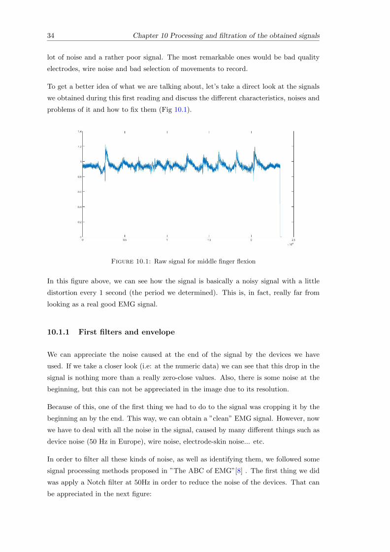
To get a better idea of what we are talking about, let’s take a direct look at the signals

we obtained during this first reading and discuss the different characteristics, noises and

problems of it and how to fix them (Fig 10.1).

Figure 10.1: Raw signal for middle finger flexion

In this figure above, we can see how the signal is basically a noisy signal with a little

distortion every 1 second (the period we determined). This is, in fact, really far from

looking as a real good EMG signal.

10.1.1 First filters and envelope

We can appreciate the noise caused at the end of the signal by the devices we have

used. If we take a closer look (i.e: at the numeric data) we can see that this drop in the

signal is nothing more than a really zero-close values. Also, there is some noise at the

beginning, but this can not be appreciated in the image due to its resolution.

Because of this, one of the first thing we had to do to the signal was cropping it by the

beginning an by the end. This way, we can obtain a ”clean” EMG signal. However, now

we have to deal with all the noise in the signal, caused by many different things such as

device noise (50 Hz in Europe), wire noise, electrode-skin noise... etc.

In order to filter all these kinds of noise, as well as identifying them, we followed some

signal processing methods proposed in ”The ABC of EMG”[8] . The first thing we did

was apply a Notch filter at 50Hz in order to reduce the noise of the devices. That can

be appreciated in the next figure:

Chapter 10 Processing and filtration of the obtained signals 35

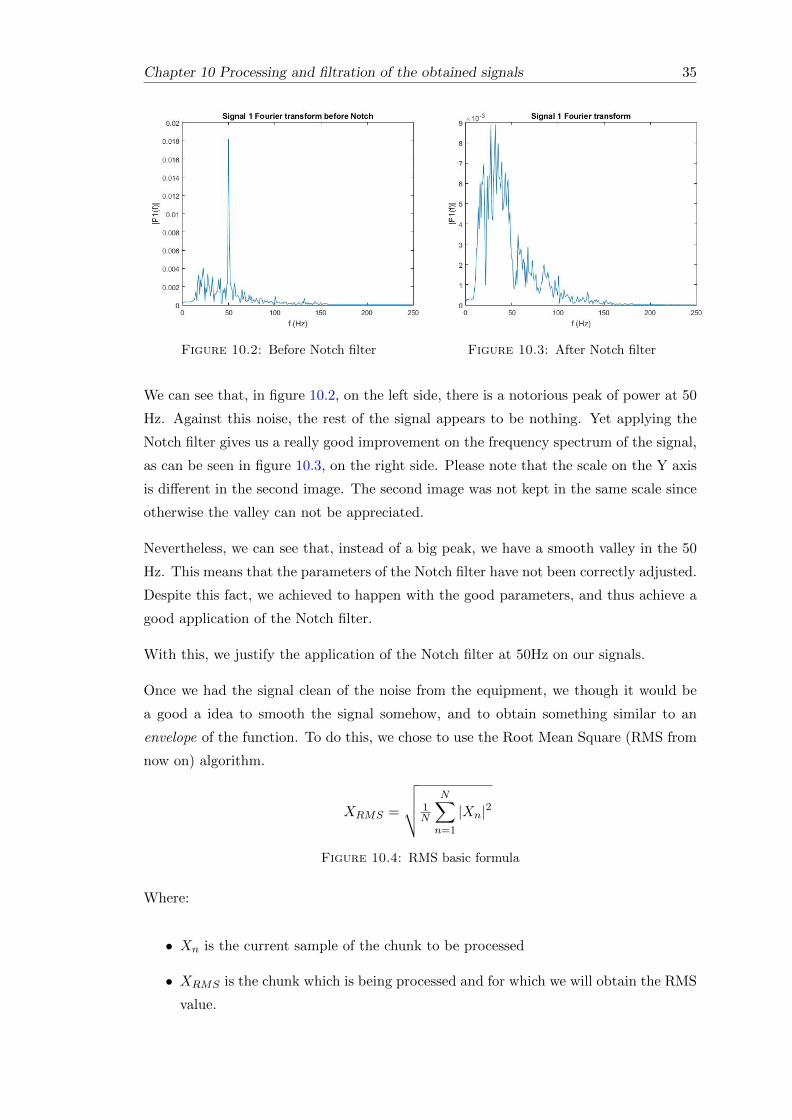
Figure 10.2: Before Notch filter Figure 10.3: After Notch filter

We can see that, in figure 10.2, on the left side, there is a notorious peak of power at 50

Hz. Against this noise, the rest of the signal appears to be nothing. Yet applying the

Notch filter gives us a really good improvement on the frequency spectrum of the signal,

as can be seen in figure 10.3, on the right side. Please note that the scale on the Y axis

is different in the second image. The second image was not kept in the same scale since

otherwise the valley can not be appreciated.

Nevertheless, we can see that, instead of a big peak, we have a smooth valley in the 50

Hz. This means that the parameters of the Notch filter have not been correctly adjusted.

Despite this fact, we achieved to happen with the good parameters, and thus achieve a

good application of the Notch filter.

With this, we justify the application of the Notch filter at 50Hz on our signals.

Once we had the signal clean of the noise from the equipment, we though it would be

a good a idea to smooth the signal somehow, and to obtain something similar to an

envelope of the function. To do this, we chose to use the Root Mean Square (RMS from

now on) algorithm.

XRMS =

√√√√ 1N

N∑n=1

|Xn|2

Figure 10.4: RMS basic formula

Where:

• Xn is the current sample of the chunk to be processed

• XRMS is the chunk which is being processed and for which we will obtain the RMS

value.

36 Chapter 10 Processing and filtration of the obtained signals

For this signal, we choosed a window size of 50 samples. At the beginning we wanted

to use the built in rms(X) function in Matlab, but it was not working well and gave us

some errors, so we implemented our own RMS function. After applying it to the signal

filtreted with the Notch filter, we obtained the results in figure 10.5

Figure 10.5: Raw signal, RMS filtered signal, and superposition of both

In the figure 10.5, we can appreciate the raw signal (already cropped), the signal after

applying the RMS filter and the superposition of both signals. Notice that there are

also some orange circles. These circles are meant to point, more or less, where the cycle

(i.e: the flexion of the finger) starts.

As expected, we have obtained an envelope of the EMG by applying this filter. However,

although it is a very beautiful signal, it is not useful for our purpose of analyzing the

nature of EMG signals and build a RT algorithm. Moreover we can see in the image

how the theoretical cycle does not correspond to the cycle in the signal in an exact way.

This shows us the delay between the order delivered by the persons (i.e: the brain) and

the actuation of the muscle.

10.1.2 Adjusting the frequency spectrum

Now, it is known that the important frequencies on the EMG spectrums are focused

between 10Hz and 200Hz, the rest can be considered noise or simply not relevant

frequencies. Therefore a low pass and a high pass filters are required in order to clean

the signal from noise.

Chapter 10 Processing and filtration of the obtained signals 37

This is why, as proposed in the papers[1],[2],[9],[10],[11], we designed a code which applies

the following filters to the signal:

• Low pass filter

• High pass filter

• Notch filter

• Moving average

In order to implement the low and high pass filters we used the Butterworth filter,

both for its good effectivity and simplicity when applied in Matlab with the function

butter(N, Wn), where N is the order of the filter and Wn the normalized cutoff frequency.

The order was set in both filters to the value 6, and the cutoff frequencies it depends on

the type of filter.

10.1.2.1 Adjusting Notch filter

Since all these filters were merged altogether into a function, it was possible to vary the

cutoff frequencies (among other parameters that we will explain later) for both low and

high pass filters. As for what the Notch filter concerns, we have already explained that

we set it at 50 Hz, however, the Matlab function iirnotch(w0, bw) as we can see has

two parameter: w0 is the cutoff frequency, and bw bandwidth. In the previous chapter

we have mentioned the impact of the parameters of this function to the output signal.

We show now in some figures the impact of different values for the bandwidth.

However, before the pictures it is important to understand how we tuned the parameters.

First we have the cutoff or Notch frequency (w0) calculated as

W0 =fnfs2

Where fn is the frequency we want to attenuate (e.g: 50 Hz) and fs is the sampling

frequency (2KHz in our case).

This value we use it for the cutoff frequency but we also use it for the bandwidth,

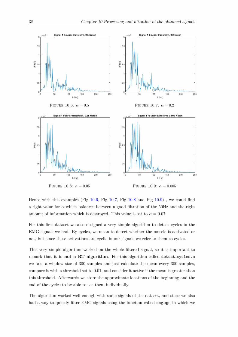
multiplying it by a factor α. This factor α is the number shown in the following pictures,

showing the impact of different α on the Notch filter:

We can see how for small values of α such as 0.05 or 0.005 we still have a peak at 50Hz,

and how for high values such as 0.5 and 0.2 we have somehow of a valley around 50Hz,

destroying some possible information.

38 Chapter 10 Processing and filtration of the obtained signals

Figure 10.6: α = 0.5 Figure 10.7: α = 0.2

Figure 10.8: α = 0.05 Figure 10.9: α = 0.005

Hence with this examples (Fig 10.6, Fig 10.7, Fig 10.8 and Fig 10.9) , we could find

a right value for α which balances between a good filtration of the 50Hz and the right

amount of information which is destroyed. This value is set to α = 0.07

For this first dataset we also designed a very simple algorithm to detect cycles in the

EMG signals we had. By cycles, we mean to detect whether the muscle is activated or

not, but since these activations are cyclic in our signals we refer to them as cycles.

This very simple algorithm worked on the whole filtered signal, so it is important to

remark that it is not a RT algorithm. For this algorithm called detect cycles.m

we take a window size of 300 samples and just calculate the mean every 300 samples,

compare it with a threshold set to 0.01, and consider it active if the mean is greater than

this threshold. Afterwards we store the approximate locations of the beginning and the

end of the cycles to be able to see them individually.

The algorithm worked well enough with some signals of the dataset, and since we also

had a way to quickly filter EMG signals using the function called emg qp, in which we

Chapter 10 Processing and filtration of the obtained signals 39

summarized all the filters explained above and included a moving average, we were ready

to take some other readings. In the figure below (Fig 10.10, we can see a very simple

flowchart describing the function:

Figure 10.10: emg qp flowchart

10.2 Second session - stronger, longer signals

As explained in the previous chapter, the signals obtained during the second session

were way better than the ones from the first session, basically because of the movement

recorded and the locations of the electrodes. Below, we can see the raw signal (cropped)

obtained during this session:

Figure 10.11: signal 1 (contractors) raw

40 Chapter 10 Processing and filtration of the obtained signals

We can see in figure 10.11 that in most of the cycles the energy of the signal grows

significantly, even for being a raw signal. However, the baseline is still pure noise, and

this means that the rest of the signal will improve if we apply the filters. Let’s take a

look at how the signal evolves after the application of the different filters.

Figure 10.12: Signal after high pass and low pass filters

In figure 10.12 the impact of applying high pass and low pass filter can be appreciated.

If we compare this signal with the raw signal, the first we must notice is that the mean

value of the filtered signal is more or less 0, instead of being around 1.

Also, if we look at the shape of the wave, we can see how some distortions and noises

between the active cycles have disappeared, and the signal is somehow symmetric on

the horizontal axis.

Nevertheless we still have the baseline as a continuous noise. One of the causes for this

issue is the noise of the equipment at 50Hz. Previously we watched what was the impact

of the Notch filter on the frequency spectrum, but have not seen yet any example of its

impact on the signal in the time domain.

In the figure below (figure 10.13), we can see the impact of the Notch filter on the signal

already filtered with both low and high pass filters. As mentioned before, it can be seen

how the noise in the baseline has diminished, as well as some of the random peaks during

the cycles.

This will be very helpful when we design the final RT algorithm, since it simplifies a

lot the detection of the activation of the muscle, and also gives us some good reference

values to calculate and detect this activation of the muscle.

It is important to remark that the filter functions in Matlab add some zeros at the

beginning and end of the signal, thus after every filter the signal needs to be cropped

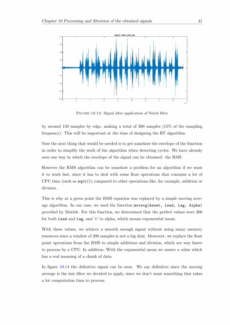
Chapter 10 Processing and filtration of the obtained signals 41

Figure 10.13: Signal after application of Notch filter

by around 150 samples by edge, making a total of 300 samples (15% of the sampling

frequency). This will be important at the time of designing the RT algorithm.

Now the next thing that would be needed is to get somehow the envelope of the function

in order to simplify the work of the algorithm when detecting cycles. We have already

seen one way in which the envelope of the signal can be obtained: the RMS.

However the RMS algorithm can be somehow a problem for an algorithm if we want

it to work fast, since it has to deal with some float operations that consume a lot of

CPU time (such as sqrt()) compared to other operations like, for example, addition or

division.

This is why at a given point the RMS equation was replaced by a simple moving aver-

age algorithm. In our case, we used the function movavg(Asset, Lead, Lag, Alpha)

provided by Matlab. For this function, we determined that the perfect values were 200

for both Lead and Lag, and ’e’ to alpha, which means exponential mean.

With these values, we achieve a smooth enough signal without using many memory

resources since a window of 200 samples is not a big deal. Moreover, we replace the float

point operations from the RMS to simple additions and division, which are way faster

to process by a CPU. In addition, With the exponential mean we assure a value which

has a real meaning of a chunk of data.

In figure 10.14 the definitive signal can be seen. We say definitive since the moving

average is the last filter we decided to apply, since we don’t want something that takes

a lot computation time to process.

42 Chapter 10 Processing and filtration of the obtained signals

Figure 10.14: Signal after moving averaging

We can see that the baseline now, at least before the first cycle, is a really low value,

close to zero if compared with the cycles. However, we can also notice that between the

cycles this value is a little higher.

Another curious characteristic of the signal is the difference between the peaks of different

cycles. It can be seen that, somehow, the pattern of a strong cycle followed by lower

once, is repeated along the signal.

These two characteristics are due to the fatigue in the muscles. When the muscle is

activated and then relaxed, it takes some time for it to get to a completely relaxed state,

and even more after a full strength fist flexion. The second phenomenon is because every

time a flexion is done, the muscle gets a little tired, hence the next flexion will not be

so strong as the previous one. However, during the recording of the signals, the patient

was reminded every some cycles to go full strength again. However, the fatigue is also a

factor of this phenomenon This can be seen in a perfect way on the 7th cycle (highest

peak of the signal).

Another impact of the fatigue during the recordings can be seen in the frequency spec-

trum, since when fatigue hits, the frequencies use to move a little to lower frequencies.

However, after all this filters and processes, the signal looks now good enough in order

to be processed by an algorithm detecting when the muscle is activated or not. Having

this so, we can start to design the RT algorithm.

Chapter 11

Designing the real time algorithm

11.1 Introduction to Real Time processing

At the time of building a RT algorithm we need to make clear some concepts. The first

thing we need to understand is what we mean by real time.

A real time algorithm or system is one that must guarantee a response to an input with

such a speed that it affects the environment at that time. In our case, this means that

the algorithm must response to the signals it is reading as if it was our very own hand.

Another thing that we must keep in mind, is the fact that now we can not work with

the whole signal, since what we want to achieve is to develop an algorithm which is able

to read, process and react to signals which are provided in real time.

In real time hardware, these signals are read using AD-converters (Analog to Digital

converters), storing the data in some memory buffer until the algorithm can read it.

This means that our algorithm can not work with a very big amount of data.

Something else that has to be bear in mind is the fact that bionic arms are devices

which the owner must be able to carry everywhere, hence a portable battery is required.

Because of this, we also need an algorithm which energy consume is low. This is somehow

bounded to the low processing time.

Knowing all this, what must be done now is to find a solution that guarantees the

following points, keeping all of them in mind:

• Very quick response

• Work with pieces of signal, instead of whole signal

43

44 Chapter 11 Designing the real time algorithm

• AD-converters timing

• Available samples of data

• Low energy consumption

However in our case, we are not going to build a physical bionic arm but carry out a

simulation, just to develop the algorithm. This means that there are some things that

can not be tested, hence we will not focus on them especially. These things are basically

AD-converter timing and low energy consumption.

Consequently, we will focus on developing an algorithm that brings a very quick response

to an estimated number of real time incoming signal chunks provided by Matlab. In

order to achieve this, we will make use of the built-in function of Matlab pause(n),

where n is the number of seconds.

11.2 Algorithm requirements and characteristics

To simplify things, we will assume that the time required by the AD-converters to obtain

the data is lower than the time required by the algorithm to process one chunk of signal.

This means that the algorithm will always have data to process in the buffer. In a real

device though, the algorithm should probably wait some time before getting the data it

needs. This would allow the CPU to just turn of until the buffer is full in order to save

energy.

The other characteristic of the algorithm that needs to be defined is the number of

samples that are going to be processed in one cycle of the algorithm; this is, the size of

a chunk in samples.

As mentioned before, every time a filter is applied to the signal, we need to crop it since

the filtering functions add some zero-close values at the beginning and at the end of

the signal. We determined that this value is around 300 samples, although it slightly

depends on the number of samples of the signal.

This means that the number of chunks that the algorithm needs must be greater than

300. However, before determining the required number of samples, we need to make a

selection of the filters that will be applied on the signal.

Chapter 11 Designing the real time algorithm 45

11.2.1 Filters selection

The filter selection is a very important step for the algorithm, since it is the step in

which, basically, the selection of filters according to all the requirements for a real time

algorithm has to be made. This means that we have to choose only the most necessary

filters in order to make the signal processable by the code.

Nevertheless, there are some filters that are completely necessary. These are basically

those which adjust the frequency spectrum of the signal. Particularly, we are talking

about:

• Low pass filter

• High pass filter

• Notch filter

In the previous chapter, we have seen how the signal improves with just these low CPU

cost algorithm: We go from a noisy raw signal full of distortions to something smooth

and clean of many of the previous noises.

The next step is to consider if we apply the RMS algorithm or not. We explained before

that float point operations are very exhaustive for the CPU, and also, it was showed

how the moving average can also achieve something similar of an envelope of the signal.

However if we are to replace the RMS by the moving average, we have to keep in mind

that we can not work with the whole signal, and before, we were using a window of

200 for this moving average. Remembering that the chunk size will be greater than 300

samples, but can not exceed this number by many samples (since we would gain lag and

lose real time effect), we have to think in an unusual way to implement this averaging

in our real time code.

However, let’s assume for the time that we will use the moving average (and we will),

and let us include it in our must-be-applied filter list. Updating our list with the values

for each filter and adding modulus, we obtain the following table:

Note that in the row of the moving average there is a *. This is because, as mentioned,

the moving average will be applied in an unusual way, and we still don’t know the

samples with which we will dispose for this averaging.

Now, we would like to remind that every time that a filter is applied, the signal needs to

be cropped in order to avoid false zero-close values. In that case, we found out that both

46 Chapter 11 Designing the real time algorithm

Filter parameters

High pass filter 20 HzLow pass filter 150 HzNotch filter 50Modulus -Moving average 200 samples*

Table 11.1: Filters applied in the real time algorithm

low and high pass filters, and also the Notch one, require 120 samples to be cropped

by filter. This is a total of 360 samples that need to be cropped in order to get a realistic

value.

11.2.2 Structure of the algorithm

Now that we know what filters will be applied it is time to discuss what will be the

structure of the real time algorithm.

It is clear that it will have a main bucle in which we will obtain chunks, process them,

obtain some values and decide, according to these values, whether the arm is activated

or not.

However, we will need to compare this values from the filtration with some other values,

otherwise there is no way we can know the difference between the two states of the arm:

activated or deactivated. This is why first of all a calibration is required.

But what should this calibration do? If we wanted to achieve an algorithm with quan-

titative results (i.e: more than one state, depending on the strength applied) we would

need to know two states on the calibration, the two limits: relaxed position and full

strength position.

Despite this fact, we will just have two states, and thus only one state must be measured

during the calibration. In our case, we chose the relaxed position as a reference point,

since we will focus on detecting activation and not deactivation of the arm. Moreover,

this state is the most common for our hands, and would allow to save battery during

repose moments.

Once the calibration is done, the main body and bucle of the algorithm can start. In

this bucle, we will need to obtain data, process it, and decide, comparing to the values

obtained during the calibration, if the arm is activated or not.

Therefore, the first step would be to obtain the data (chunk) to be processed. Then a

function that applies the filters mentioned in table 11.1 (except for the moving average)

Chapter 11 Designing the real time algorithm 47

will be called. With this we will obtain a processed chunk of data. This means that we

will have a bunch of processed samples, but with this we can not directly work; we need

to obtain some characteristics from this chunk. There is when we apply the mean: We

apply the Matlab built-in function mean(A) to the processed chunk.

This way we obtain a value which can be compared to the reference values (values

obtained during calibration). However, using only one chunk of data is not a good

option since maybe this chunk is an exception within the set of the previous chunks.

By exception we mean a distortion or noise that alters the current state of the signal

seeming it to be what it is not. For example, we could be in a moment of repose and a

noise caused by friction or electromagnetic waves alters our signal creating a very brief

peak. This is known as a false positive.

Consequently, some previous values are used also to decide the current state of the arm

in order to avoid false positive and to bear in mind the previous state of the arm. This

number was set to 5 chunks in total. The response time delay will be discussed in the

detailed explanation of the algorithm

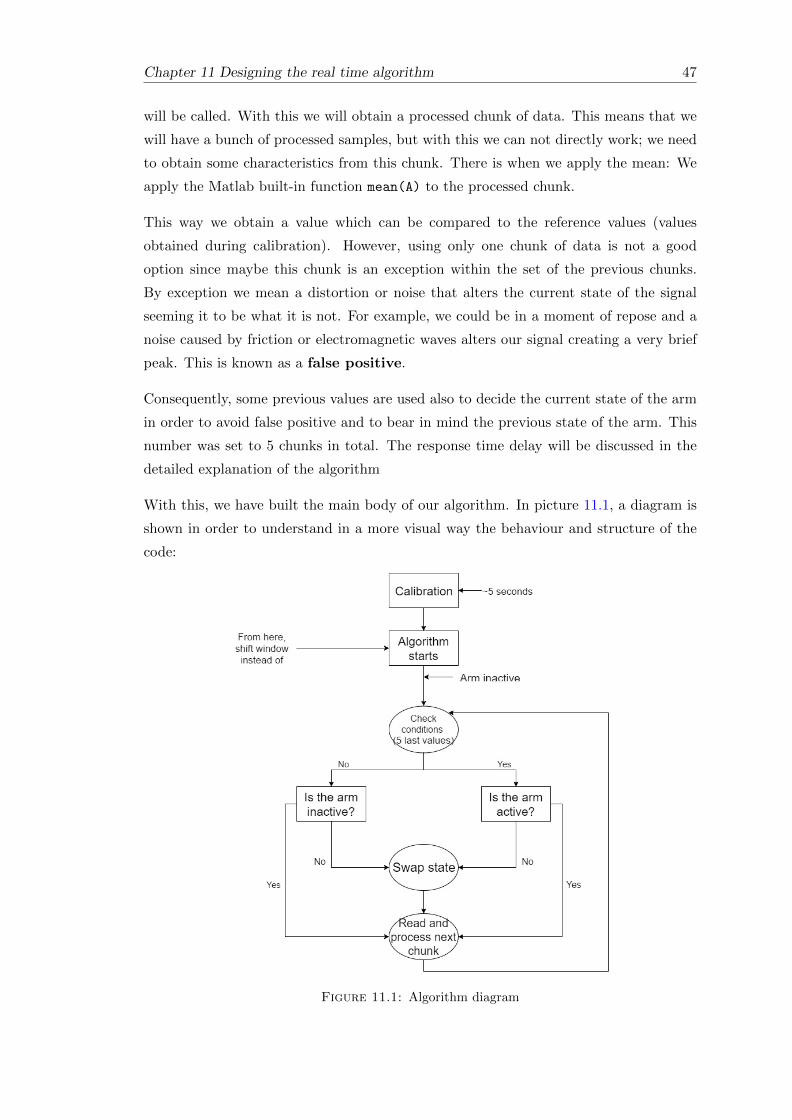
With this, we have built the main body of our algorithm. In picture 11.1, a diagram is

shown in order to understand in a more visual way the behaviour and structure of the

code:

Figure 11.1: Algorithm diagram

48 Chapter 11 Designing the real time algorithm

Now we still have to answer to the question: what number of samples will a chunk have?

In order to solve this problem, we focused on the percentages of one second, which is

the same as saying, focusing on percentages of the sampling frequency.

At the beginning, 500 samples were used, but with this number, the mean had a little

lack of meaning. More samples were needed in order for the algorithm to take into

account greater amounts of data.

Therefore, the number of samples was set to 600. It is important to remark that from

these 600 samples, 360 samples are going to be cropped because of the filtering. Hence

this leaves us with a total of 240 effective samples, which is around the 10% of

the sampling frequency. This leaves us with a time delay of 0.3 seconds per chunk.

However, as has been mentioned, the number of effective samples is 240, therefore the

real delay is around 0.12 seconds.

Nevertheless, this is not the exact delay value, since as we have already mentioned, more

than one chunk is used by the decision. The final result is 5 chunks, which means that

the final time delay is 0.6 seconds.

11.3 Algorithm detailed explanation

The first thing to mention is that in the purpose of this section is not to explain the

code line per line and explain why every command was used but to explain how the

main functions of the algorithm work. To take a direct look at the code, please address

to Appendix B.

In order to explain the algorithm in a proper way, the different functions will be detailed

in the order they appear in the algorithm. This way, one can follow the explanation in

a chronological way looking at the main algorithm.

11.3.1 Calibration - emg calibrate.m

In this function of the code we want to obtain certain aspects and characteristics of the

repose state of the arm in order to have some values with which the processed chunks

can be compared.

To do this, we will work with frames of 600 samples as explained before. In the case of

the calibration, the window shift will be 600 samples as well, which means that every

chunk has completely different samples.

Chapter 11 Designing the real time algorithm 49

Now, we thought that a calibration of 5 seconds would be enough to ensure a good

and reliable reference values. However, which values do we want to obtain? In the first

version of the algorithm, only the mean of all the processed chunks (including the mean

for every chunk) was collected.

Nevertheless, after some readings and considerations, we realised that a simple mean

was not enough to guarantee a truthful result. Thus, the standard deviation (calculated

with the Matlab built-in function) was included. Note that the standard deviation is

the one calculated out of the mean of all processed chunks.

11.3.2 Processing chunks - filter chunk.m

In this section not only the filtration of the chunks will be explained but also some

characteristics of the main bucle.

The first thing that requires explanation is the way the chunks are used in this part

of the code. In the calibration, the window shift was 600 so that a sample was never

reused in another chunk. In this part of the code though, the window shift is just 200

samples, meaning that from the total 600 samples of a chunk, 400 are taken from the

last chunk.

This is done so that every chunk keeps some part of the previous chunk in order to avoid

false positives and to keep somehow the slope of the signal in every chunk. In other

words, we always keep some information from the past. Having said that, we can now

focus on the function itself.

If we compare the code we find in this function with the code in the file emg qp.m we

can see that there is not much difference. Basically we take the chunk from both signals

and apply the filters we mentioned the ”Algorithm requirements and characteristics”

section, for exception of modulus and moving average, which are applied afterwards as

we already explained.

11.3.3 Taking decisions - check active.m

This is the most important part of our algorithm, in which the activation of the arm is

decided based on the data we have. It is important to remark again that we keep the

last 5 values that have been processed. This values are stored in the vectors values 1

and values 2 for the first and second signal respectively. At the first iteration, this

vectors are filled with the reference values obtained from the calibration.

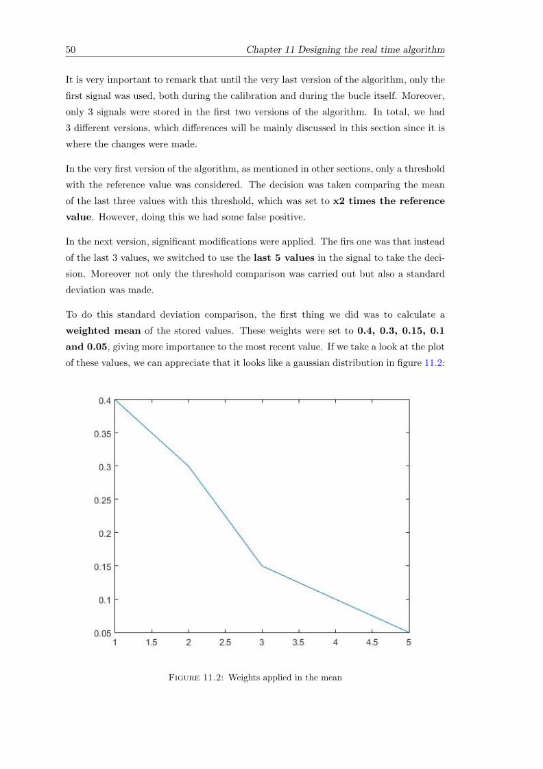
50 Chapter 11 Designing the real time algorithm

It is very important to remark that until the very last version of the algorithm, only the

first signal was used, both during the calibration and during the bucle itself. Moreover,

only 3 signals were stored in the first two versions of the algorithm. In total, we had

3 different versions, which differences will be mainly discussed in this section since it is

where the changes were made.

In the very first version of the algorithm, as mentioned in other sections, only a threshold

with the reference value was considered. The decision was taken comparing the mean

of the last three values with this threshold, which was set to x2 times the reference

value. However, doing this we had some false positive.

In the next version, significant modifications were applied. The firs one was that instead

of the last 3 values, we switched to use the last 5 values in the signal to take the deci-

sion. Moreover not only the threshold comparison was carried out but also a standard

deviation was made.

To do this standard deviation comparison, the first thing we did was to calculate a

weighted mean of the stored values. These weights were set to 0.4, 0.3, 0.15, 0.1

and 0.05, giving more importance to the most recent value. If we take a look at the plot

of these values, we can appreciate that it looks like a gaussian distribution in figure 11.2:

Figure 11.2: Weights applied in the mean

Chapter 11 Designing the real time algorithm 51

Once the mean is calculated, it is afterwards compared to the reference value plus some

standard deviations: ref1 + 3*std1; where ref1 is the reference value and std1 is the

standard deviation of the calibration.

The threshold was also modified, and instead of calculating the mean and then compare,

just the sum of the values is performed and then compared to a value based on the

reference value. In this version, the value is set to (4*(3*ref1)). A 12 is not put since

this value was obtained by adjusting multiplications of the value obtained from 3*ref1.

Another thing that must be explained is that the deciding function has two cases in it.

As can be seen in the code, within the two conditions, the comparisons performed are

the same but with different values as thresholds. This is done because while the strength

is carried out, the muscle has ups and downs. If we take a look at figure 10.14 from the

previous chapter, we can see how one cycle starts with a peak, which is followed by a

valley and ends with another peak. With these low values for deactivation of the arm,

we prevent the hand to deactivate during these valleys.

Another solution would be to just reduce the activation values, but this would suppose

a greater number of false positives, which, with this implementation of the algorithm

was reduced to 1.

However, until this point only one signal was used to perform the decision, and since

we have two signals, it would be useful to use the information provided by both of

theme. Therefore the next step was to join the two signals and perform tests based on

parameters from both.

In order to implement these changes, the first thing to do was to thing of a way to

merge the two signals. The first thing that was tried was to do the mean between the

two values from the two different signals and compare them to the mean of the reference

values, but that would suppose too much computation time and thus was discarded.

Also the addition of the two signals was considered, but then changes on the reference

points and comparison systems would had been to be applied as well.

Therefore we opted to just compare the signals separately and focus the decision on the

activation by one of them. However, we wanted to add an statistical test to the check

function because it brings information about the similarity of the chunk with the resting

value, and hence it can be used for future work to do a quantitative algorithm. To do

so, we used the Matlab built-in function ttest2(x, y).

This function assumes that both values are composed by the same distribution (e.g:

gaussian) and compares, within a confidence range, if this null hypothesis is true. This

function returns two values: [h,p]. If h=0 it accepts the null hypothesis for normal

52 Chapter 11 Designing the real time algorithm

distributions with equal means, otherwise if h=1 the test rejects the null hypothesis

at the p-value for error level. And p-value (p of the test), which tells the probability

of observing the statistic test as more extreme than the observed value under the null

hypothesis (i.e: the test error of rejection of the null hypothesis).

In our case, only p was used, independently from the state of the arm, we assumed that

it meant activated if it was greater than 10−4. This value was statistically determined

and means that the difference between the signal exists (significant difference at the

p-value) and the probability of this decision is greater than 99.99% which means a very

high significance.

Note also that to calculate these last p value, we used the addition of the two signals

compared with the mean of the references. This is the main reason why the p value

threshold is set that low.

The version of the algorithm combining the two signals, carrying state-dependent deci-

sions on direct threshold and std based thresholds; and independent comparison with p

value from statistical test, is the the final version of the algorithm. The number of false

positives with this version was reduced to 0 for the second session signals.

11.4 Other aspects of the algorithm

As can be seen in the algorithm, besides the calculations needed for the bionic arm

simulation, there a few more things that are done. One of these things is the recording

of the initial and ending positions of the cycles.

This was done in order to analyze the nature and characteristics of the EMG especially

when the muscles are activated. Some characteristics worth to investigate with this ad-

ditional tool is the frequency spectrum and fatigue on the active signals. With this data

(cycles from the real time algorithm) one can use the function normalize cycles(cycles,

s1, s2) where, for better results, s1 and s2 should be the signals avS1 and avS2 from

emg qp.m

Part III

Results, conclusions and future

work

53

Chapter 12

Results and conclusions

12.1 Results

12.1.1 About EMG

During the development of this project, the main thing which with we have worked was

EMG signals. Therefore, it is important to start the results section talking about what

has been obtained in this matter during this thesis.

Since we had different sessions for recording EMG signals, and every session had some-

thing that the other did not have, we have been able to work with some different types

of signals. Not only this, but also we learned some good ways and methods in order to

obtain good signals to work with.

Moreover, the filtration applied to this signals was completely satisfactory, since it

allowed the algorithm to achieve its goals. Regarding the goals specified over EMG

signals, we have learned the nature and characteristics of them, and we have learned

how to filter these signals in order to obtain something clear in a few steps and in quite

a fast and efficient way.

During the explanation of the project, the evolution of the EMG signals could be appre-

ciated, either by the changes realised in the recording methods or by the filters applied.

In addition, we have learned the impact of the fatigue on the EMG signals, and thus

some measures in order to apply it to the algorithm has been considerated. We will talk

about this in future work.

Therefore, the goals as for the EMG signals were successfully achieved.

55

56 Chapter 12 Results and conclusions

12.1.2 About the RT algorithm

The algorithm that has been developed during the project has successfully achieved the

requisites exposed as main goals of the project, this is, being able to recognise simple

movements for a bionic hand limbs from EMG signals.

Moreover, the platform that has been used to develop such algorithm, is not meant to

design real time algorithms, and, despite this fact, the algorithm is capable to run at

real time without any appreciable delay from the human sight. It is true that Matlab

carries out multithread operations automatically, but some cheap microchip can run

multithread operations as well.

The results for the real time simulation (this is, with the first dataset) were very sat-

isfactory. In the figure 12.1 the signal read by the algorithm is shown. This signal is

the resultant signal from the processing applied in the algorithm (mean ans modulus

included) for the signal from the forearm contractors.

Figure 12.1: Signal interpreted by the algorithm

In the case of figure 12.1 only one false positive was detected as positive (marked with

red shadow) and one relaxed position was determined as active (the period between the

first and the second cycle). The rest of small peaks between cycles were successfully

detected as false positive, and hence still detected as relaxed positions.

However, this relaxed period between the two signals has a really high value. This is

very rare for a noise, so most likely it was caused by a bad relaxed position by the

Chapter 12 Results and conclusions 57

patient. Regarding the false positive detected as active value, we can say that it is quite

a high peak (rarely seen) and that is the reason why it was detected as positive.

With this results we can say that the algorithm that has been developed has success-

fully reach the requirements stated at the beginning of this document.

12.2 Conclusions

As in the previous chapter about results, we will start talking about what we have

learned about EMG signals, and afterwards we will talk about the code.

12.2.1 Conclusions about EMG signals

The first thing to mention about this signals is that, as any other physiological signal, it

is by default a very noisy signal. As we could see in the figures while we were describing

the reading sessions, we could see how the first signals were full of noise and distortion.

As we discussed this could be caused either by the accidents such as skin, muscle, and

other biologic factor noises, cable noise, bad electrode contact... etc. This is regard-

ing the noise. Other factors that can cause this poor signals are the wrong choice of

movement to record, or a not high performance equipment.

However the biological accidents and many of the other noises were completely proven

as false during the second session. This teaches us that the set of movements to record,

as well as the way they are recorded (electrode placements) are very important at the

time to obtain clear signals.

Nevertheless, even in these signals we could still find some constant noise. This noise is

caused mainly by the equipment and the cables. This means that the equipment plays

also a very important role on taking good signals. One way we could solve this issue is

to use preamplified electrodes to reduce the cable noise, or even contact-less electrodes.

Another solution, but a little way more drastic is to replace the whole equipment by a

high performance equipment, but this suppose a big amount of money.

Also, working with such good equipment can have, depending on the point of view, a

bad impact on this thesis. This is, if we work with very high-tech devices, first we are

raising by default the price of a physical limb, and plus, this equipment is probably so

big that it is impossible to fit into a portable device.

Therefore, the fact of working with rather bad signals can be seen even as a positive

point for the thesis, since in a portable, low budget and energy optimal device, the

58 Chapter 12 Results and conclusions

signals that can be used because of the equipment available are rather low. Hence, our

algorithm can work properly on a real device.

Summing up, the concepts learned during this thesis about EMG signals, is that they

are tricky signals, that highly depend on the equipment and procedure at the time of

being recorded in order to obtain a clean signal. Despite this, the fact that not excellent

signals were used, makes our algorithm suitable for a real bionic limb.

12.2.2 Conclusions about the algorithm

Real Time algorithms are complicated de per se, but when they get mixed with signal

processing and EMG signals, the thing gets even worse. However, during the develop-

ment of the thesis, the algorithm we built achieved the main goal of the project, which

was to recognise basic movements of a hand.

We have learned how to design a software which is able to study statistic properties

from calibration values and afterwards use this values as reference for decision functions

which worked with signals obtained and processed in real time.

12.3 Future work

Regarding the future work, most of the work is based on the algorithm and not in the

EMG signal processing. The question to say this is that, if more filters are to be applied

to the EMG signals, it would have a negative time on the real time process. Either this

or raise the price of the product, since more powerful components would be required.

Therefore let us talk about what we think it can be improved in our algorithm. Until

now, we have an algorithm which is capable to detect a very basic move. This is good,

since it does it pretty well, but it is still a binary action; this is, for now, we just have

two positions for our hand: open or closed. Therefore one of the things to be improved

in the algorithm is to turn this binary state into a gradual state.

The strength one delivers when grabing a bottle of whater is not the same as the strength

delivered when holding a heavy grocery bag. When you drink from a bottle of water,

you do not want to struggle it, bot just grab it. This is why this step is really important

in a future work.

Another issue that is very important is the set that compose the movements of our

hand. Closing and opening the fist is important, but in our daily life, we use our hands

in many other different ways. It is true that, using our algorithm, many basic functions

Chapter 12 Results and conclusions 59

can be done without problem since many of these activities consist on one hand holding

an object and the other hand interacting with it (such as when someone whisks).

Because of this, it would be very interesting and important to add different types of

movements to the algorithm. Nevertheless, this a very hard work. We would like to

remin that the first attempt to register EMG signals was moving fingers separately, but

the signals looked almost the same. Hence this is not an easy work.

Another thing that could be used to improve the functionality of the prosthesis is the

study of the fatigue. During the different signals we have seen the impact of the fatigue

on the signal shape and power. Statistical properties on the evolution and characteristics

of this fatigue could be used in order to improve the performance of a prosthesis. It

could be even possible to delete the fatigue in the resultant movement. With this we

mean, act as if the muscles were not tired and perform more strength than what is being

read from the muscles.

One important thing which we consider important is the translation of the code. Now

we have a code implemented in Matlab, which is a great application for simulation,

study of the signals, and first developments. But if this algorithm has to work with real

time platforms, it would be really interesting to translate this code into a more suitable

language for real time devices, such as C, C++ or Python.

Appendix A

Extra figures

A.1 Project budget

61

62 Appendix A Extra figures

A.2 Lab equipment

Figure A.1: NI ELVIS II

Figure A.2: EKG sensor

Figure A.3: Dynamometer

Appendix B

Matlab code

B.1 EMG quick processing function - emg qp.m

1 % Script for quick EMG processing (NO DYNAMOMETER)

2 %

3 % emg_qp quickly process and EMG signal to have some feedback from it when

4 % captured in the lab. The parameters are the following:

5 %

6 % - filename: filename of the file containing the EMG

7 % - sf: samplig frequency of the signal

8 % - hp_freq: high pass frequency

9 % - lp_freq: low pass frequency

10 % - wsize: window size for filtering

11 % - f_sr: Fourier sampling rate

12 % - show_evo: if true , shows evolution of signal after filters

13 function [S1, S2 , FS1 , FS2 , avS1 , avS2] = emg_qp(filename , sf, hp_freq , ...

14 lp_freq , wsize , f_sr , show_evo)

15 % Reading signals

16 load(filename );

17 % Signals are cropped to avoid lab equipment activation and

18 % deactivation noise.

19 S1 = biosignalDev2_ai0.Data;

20 S1 = S1 (100:( size(S1) -200));

21 S2 = biosignalDev2_ai7.Data;

22 S2 = S2 (100:( size(S2) -200));

23

24 if (show_evo)

25 figure;

26 plot(S1);

27 title('Signal 1 RAW');

28 figure;

29 plot(S2);

30 title('Signal 2 RAW');

31 end

32

63

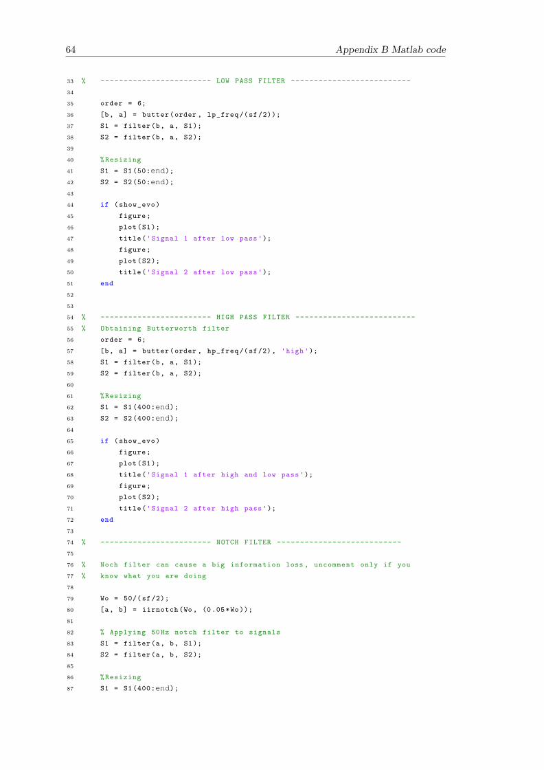
64 Appendix B Matlab code

33 % ------------------------ LOW PASS FILTER --------------------------

34

35 order = 6;

36 [b, a] = butter(order , lp_freq /(sf/2));

37 S1 = filter(b, a, S1);

38 S2 = filter(b, a, S2);

39

40 %Resizing

41 S1 = S1(50:end);

42 S2 = S2(50:end);

43

44 if (show_evo)

45 figure;

46 plot(S1);

47 title('Signal 1 after low pass');

48 figure;

49 plot(S2);

50 title('Signal 2 after low pass');

51 end

52

53

54 % ------------------------ HIGH PASS FILTER --------------------------

55 % Obtaining Butterworth filter

56 order = 6;

57 [b, a] = butter(order , hp_freq /(sf/2), 'high');

58 S1 = filter(b, a, S1);

59 S2 = filter(b, a, S2);

60

61 %Resizing

62 S1 = S1(400:end);

63 S2 = S2(400:end);

64

65 if (show_evo)

66 figure;

67 plot(S1);

68 title('Signal 1 after high and low pass');

69 figure;

70 plot(S2);

71 title('Signal 2 after high pass');

72 end

73

74 % ------------------------ NOTCH FILTER ---------------------------

75

76 % Noch filter can cause a big information loss , uncomment only if you

77 % know what you are doing

78

79 Wo = 50/(sf/2);

80 [a, b] = iirnotch(Wo, (0.05*Wo));

81

82 % Applying 50Hz notch filter to signals

83 S1 = filter(a, b, S1);

84 S2 = filter(a, b, S2);

85

86 %Resizing

87 S1 = S1(400:end);

Appendix B Matlab code 65

88 S2 = S2(400:end);

89

90 if (show_evo)

91 figure;

92 plot(S1);

93 title('Signal 1 after notch filter ');

94 figure;

95 plot(S2);

96 title('Signal 2 after notch filter ');

97 end

98

99

100 % ------------- DELETING EXTREME VALUES AND PLOTTING ----------------

101 % S1 = emg_rms(S1 , wsize);

102 % S2 = emg_rms(S2 , wsize);

103 % Deleting 0 close values at beginning and end

104 S1 = delete_zeros(S1, false );

105 S2 = delete_zeros(S2, false );

106

107 % Cropping signals again to avoid filtering initial noise

108 S1 = S1 ';

109 % S1 = S1(350: size(S1));

110 S2 = S2 ';

111 % S2 = S2(400: size(S2));

112

113 FS1 = fft(S1 , f_sr);

114 FS2 = fft(S2 , f_sr);

115

116 % -------------------- Plotting filtered signals --------------------

117 figure;

118 plot(S1);

119 title('Signal 1: Extensors ');

120 figure;

121 plot(S2);

122 title('Signal 2: Wirst tendoms ');

123

124 cor = xcorr(S1, S1);

125 figure;

126 plot(cor);

127 title('Cross correlation between signal 1 and signal 2');

128

129 % -------------------Plotting fourier transforms --------------------

130 % First , define axis as power and frequency

131 sfs1 = size(FS1);

132 sfs2 = size(FS2);

133

134 ps1 = abs(FS1/sfs1 (1));

135 ps1 = ps1 (1: sfs1 (1)/2+1);

136 ps1(2:end-1) = 2*ps1(2:end-1);

137

138 ps2 = abs(FS2/sfs2 (1));

139 ps2 = ps2 (1: sfs2 (1)/2+1);

140 ps2(2:end-1) = 2*ps2(2:end-1);

141

142 freq_dom_s1 = sf*(0:( sfs1 (1)/2))/ sfs1 (1);

66 Appendix B Matlab code

143 freq_dom_s2 = sf*(0:( sfs2 (1)/2))/ sfs2 (1);

144

145 % Now plotting

146 figure;

147 plot(freq_dom_s1 (1: int32(end/4)), ps1(1: int32(end /4)));

148 title('Signal 1 Fourier transform ');

149 xlabel('f (Hz)');

150 ylabel('|P1(f)|');

151 figure;

152

153 plot(freq_dom_s2 (1: int32(end/4)), ps2(1: int32(end /4)));

154 title('Signal 2 Fourier transform ');

155 xlabel('f (Hz)');

156 ylabel('|P1(f)|');

157

158 % -------------------- Moving Average ------------------------

159 avS1 = movavg(abs(S1), 200, 200, 'e');

160 avS2 = movavg(abs(S2), 200, 200, 'e');

161

162 figure;

163 plot(avS1);

164 title('Signal 1 moving average ');

165

166 figure;

167 plot(avS2);

168 title('Signal 2 moving average ');

169 end

Appendix B Matlab code 67

B.2 Algorithm main body - ttest RT EMG processing.m

1 % Bionic Hand Real Time Simulation script

2 % Author: Ferran Olid Dominguez

3

4 % This file is part of the Bachelor thesis carried on by Ferran Olid

5 % Dominguez , and is protected under BSD license. Therefore , any use or

6 % distribution of this code , partial or complete , must recognise the

7 % credits to the original author.

8

9 % Given an array containing EMG signals from a huma forearm , this script

10 % processes these signals in order to detect wether the muscles are active

11 % or not , hence recognising when the fist is closed or not. The signals

12 % used in this thesis are EMG signals recorded from the flexo carpum

13 % muscles (S1) and smaller forearm extensors (S2).

14 % The signal S3 is the reading of a Dynamometer recording the strength (in

15 % Newtons) of the fist when it closes. It can be used to relate the

16 % strength of the muscle signals with the final strength of the arm.

17

18 clear;

19 % Declaring general variables

20 sf = 2000; % Sampling frequency

21 filename = '2016 _05_04_2ecg_hand_2.mat ';

22 lp_freq = 150; % Low pass frequency

23 hp_freq = 20; % High pass frequency

24 wsize = 50; % window size

25 chunk_size = 600; % RT simulation chunk size

26 window_shift = 200; % After calibration , shifting of the window

27 calib_time = 5; % Seconds of calibration

28 maxmean = 0; % Mean of the maximums

29 DEBUG = true; % Debug flag

30 cycles = zeros(1, 2); % Cycle storage

31

32 % Declaring other variables

33 max_counter = 1;

34

35 % Reading data from files

36 [S1 , S2] = read_signals(filename );

37 hand = imread('images/hand.png ');

38 fist = imread('images/fist.png ');

39

40 % Starting RT simulation

41 % First seconds are for resting position calibrations

42 disp( sprintf( 'Calibrating... '));

43 iterations = calib_time /( chunk_size/sf);

44 [rest_pos1 , rest_pos2 , std1 , std2] = emg_calibrate(S1, S2, iterations , ...

45 lp_freq , hp_freq , sf, chunk_size );

46 disp( sprintf( 'Calibration done!') );

47 disp( sprintf( 'Starting bionic hand algorithm... ') );

48

49 if (DEBUG)

50 rest_pos1;

51 std1;

68 Appendix B Matlab code

52 end

53

54

55 if(~ DEBUG)

56 figure;

57 imshow(hand);

58 hold on;

59 end

60 ssample = size(S1);

61 active = false;

62 values_1 = [1, rest_pos1 , rest_pos1 , rest_pos1 , rest_pos1 ];

63 values_2 = [1, rest_pos2 , rest_pos2 , rest_pos2 , rest_pos2 ];

64 monitor = 0; % Stores mean , processed values from EMG signal

65 n = 0;

66 if (DEBUG)

67 figure;

68 plot(monitor );

69 hold on;

70 end

71 onval = 0;

72 offval = 0;

73

74 for i = (iterations*chunk_size ): window_shift:ssample

75 % Getting actual value(s)

76 [actval1 , actval2] = filter_chunk(S1(i:int32(i+chunk_size )), ...

77 S2(i:int32(i+chunk_size )), lp_freq , hp_freq , sf);

78 values_1 (1) = mean(actval1 );

79 values_2 (1) = mean(actval2 );

80

81 if (DEBUG)

82 monitor = [monitor , mean(actval1 )];

83 plot(monitor , 'b');

84 end

85

86 if (active)

87 % Arm is active here --------------------------------------------

88 if (~ ttest_check_active(values_1 , values_2 , rest_pos1 , rest_pos2 ,...

89 std1 , std2 , true))

90 active = false;

91 if (~DEBUG)

92 do_move ()

93 imshow(hand);

94 end

95 disp( sprintf( 'Hand deactivated!') );

96 offval = i;

97 % Recording cycle

98 cycles(end , :) = [onval , offval ];

99 cycles = [cycles; 0, 0];

100 end

101 values_1 = update_values(values_1 );

102 values_2 = update_values(values_2 );

103 % Updating maximum

104 maxmean = (maxmean *( max_counter -1) + values_1 (1))/( max_counter );

105 max_counter = max_counter + 1;

106 else

Appendix B Matlab code 69

107 %Arm is inactive here -------------------------------------------

108 if (ttest_check_active(values_1 , values_2 , rest_pos1 , rest_pos2 , ...

109 std1 , std2 , false))

110 active = true;

111 if (~DEBUG)

112 do_move ()

113 imshow(fist);

114 end

115 disp( sprintf( 'Hand activated!') );

116 onval = i;

117 n = n+1;

118 if (DEBUG)

119 n

120 end

121 end

122 values_1 = update_values(values_1 );

123 values_2 = update_values(values_2 );

124 end

125 pause(window_shift/sf); % RT here

126 end

127

128 % Setting positions on cycle matrix

129 cycles = cycles.*window_shift +( iterations*chunk_size );

70 Appendix B Matlab code

B.3 Reading signals - read signals.m

1 function [ S1, S2 ] = read_signals( filename )

2 %READ_SIGNALS Read emg signals from files

3

4 load(filename );

5

6 % Cutting ending of the signals (device start and stop noise)

7 S1 = biosignalDev2_ai0.Data;

8 S1 = S1 (100:( size(S1) -200));

9 S2 = biosignalDev2_ai7.Data;

10 S2 = S2 (100:( size(S2) -200));

11

12 end

B.4 Calibration function - emg calibrate.m

1 function [ rest_pos1 , rest_pos2 , std1 , std2 ] = emg_calibrate( S1, S2, ...

2 iterations , lp_freq , hp_freq , sf, chunk_size )

3 %EMG_CALIBRATE Calibrates EMG signals

4 % Given two EMG signals , this function calculates the means of some

5 % preprocessed chunks of the EMG data. Actually , it corresponds to

6 % around 5 seconds of data (i.e: 10k samples)

7

8 rest_pos1 = 0;

9 rest_pos2 = 0;

10 acc1 = [1];

11 acc2 = [1];

12 for i = 1: iterations

13 j = (i-1)* chunk_size +1;

14 j1 = i*chunk_size;

15 [fs1 , fs2] = filter_chunk(S1(j:j1), S2(j:j1), lp_freq , hp_freq , sf);

16 mfs1 = mean(fs1);

17 mfs2 = mean(fs2);

18 rest_pos1 = rest_pos1 + mfs1;

19 rest_pos2 = rest_pos2 + mfs2;

20 acc1(i) = mfs1;

21 acc2(i) = mfs2;

22 acc1 = [acc1 , 0];

23 acc2 = [acc2 , 0];

24 end

25

26 rest_pos1 = rest_pos1 / iterations;

27 rest_pos2 = rest_pos2 / iterations;

28 std1 = std(acc1(1:end-1));

29 std2 = std(acc2(1:end-1));

30 end

Appendix B Matlab code 71

B.5 Processing chunk - filter chunk.m

1 function [ fs1 , fs2 ] = filter_chunk( S1, S2, lp_freq , hp_freq , sf )

2 %FILTER_CHUNK Filters a chunk of EMG data

3 % Given a chunk of EMG data , this function applies the next

4 % signal filters:

5 %

6 % - Low pass filter at lp_freq

7 % - High pass filter at hp_freq

8 % - Notch filter at 50 Hz (change to 60Hz for american countries)

9

10

11 % ------------------------ LOW PASS FILTER --------------------------

12

13 order = 6;

14 [b, a] = butter(order , lp_freq /(sf/2), 'low');

15 S1 = filter(b, a, S1);

16 S2 = filter(b, a, S1);

17

18 %Resizing

19 S1 = S1(120:end);

20 S2 = S2(120:end);

21

22 % ------------------------ HIGH PASS FILTER --------------------------

23 % Obtaining Butterworth filter

24 order = 6;

25 [b, a] = butter(order , hp_freq /(sf/2), 'high');

26 S1 = filter(b, a, S1);

27 S2 = filter(b, a, S1);

28

29 % Resizing

30 S1 = S1(120:end);

31 S2 = S2(120:end);

32

33 % --------------------- NOTCH FILTER ----------------------------

34 Wo = 50/(sf/2);

35 [a, b] = iirnotch(Wo, (0.05*Wo));

36

37 % Applying 50Hz notch filter to signals

38 S1 = filter(a, b, S1);

39 S2 = filter(a, b, S2);

40

41 % Resizing

42 S1 = S1(120:end);

43 S2 = S2(120:end);

44

45 % Transposing and "absoluting" signals

46 S1 = abs(S1 ');

47 S2 = abs(S2 ');

48

49 % figure;

50 % plot(S1);

51 % title('Signal 1: Extensors ');

72 Appendix B Matlab code

52 % figure;

53 % plot(S2);

54 % title('Signal 2: Wirst tendoms ');

55

56 fs1 = S1;

57 fs2 = S2;

58 end

B.6 Value updater - update values.m

1 function [ values ] = update_values( vals )

2 %UPDATE_VALUES Update values in the vals array

3 % In this case , this function is just a shifting of the values in the

4 % array. However in a real RT algorithm , it should be the one in

5 % charge of reading the values from the sensors and update them in the

6 % vectors of the algorithm

7

8 values = [1, vals(2:end)];

9 end

Appendix B Matlab code 73

B.7 Deciding function - ttest check active.m

1 function [ active ] = ttest_check_active( vals1 , vals2 , ref1 , ref2 , std1 , ...

2 std2 , actived )

3 %CHECK_ACTIVE Returns whether the arm is active or not

4 % This function is the one that decides wether the robotic arm should activate

5 % or not. To do this it checks the values stored in the "vals" array , and do

6 % some tests on them , such as scope , threshold values and std. Also , in

7 % the ttest_ version , statistical test is performed and used to

8 % determinate the activation of the hand

9

10 % variables

11 conditions = zeros(1, 3);

12 weights = [0.4 , 0.3, 0.15 , 0.10 , 0.05];

13

14 refa=ones (1 ,5)* ref1;

15 refb=ones (1 ,5)* ref2;

16

17 [h,p]= ttest2(abs(vals1+vals2),mean([refa; refb ]));

18

19 % Checking threshold and std tests

20 if (~ actived)

21 conditions (1) = (sum(vals1) > (4*(3* ref1 ))) || ...

22 (sum(vals2) > (4*(3* ref2 )));

23 conditions (2) = (sum(weights .* vals1) > (ref1 + 3*std1)) || ...

24 (sum(weights .* vals2) > (ref2 + 3*std2 ));

25 else

26 conditions (1) = (sum(vals1) >= (2* ref1)) || (sum(vals2) >= (2* ref2 ));

27 conditions (2) = (sum(weights .* vals1) >= (ref1 + 1*std1)) || ...

28 (sum(weights .* vals2) >= (ref2 + 1*std2 ));

29 end

30

31 % Checking ttest value

32 if p < 0.0001

33 conditions (3) = 0;

34 else

35 conditions (3) = 1;

36 end

37 active = (sum(conditions) >= 3);

38

39 % This tells which muscle is the stronger (remove semicolon)

40 check =[[ vals1+vals2 ]/[vals1 -vals2 ]];

41

42 end

74 Appendix B Matlab code

B.8 Normalize cycles - normalize cycles.m

1 function [ out1 , out2 ] = normalize_cycles( cycles , s1 , s2 )

2 %NORMALIZE_CYCLES Normalize cycles of EMG data both in width and power

3 % Given two signals , s1 and s2, and a vector with initial and ending

4 % positions for cycles , cycles , this function normalize the cycles from

5 % signals s1 and s2 located within the frames specified in cycles.

6

7

8 % First thing is to look for the widest cycle

9 max_length = 0;

10 max_loc = 0;

11 aux = cycles(:, 2) - cycles(:, 1);

12

13 size_cycles = size(cycles) - 1;

14

15 out1 = zeros (2000 , size_cycles (1));

16 out2 = zeros (2000 , size_cycles (1));

17

18 maxpow1 = max(s1);

19 maxpow2 = max(s2);

20

21 % Normalizing

22 for i=1:( size(cycles )-1)

23 % Normalizing length

24 aux = s1(cycles(i, 1): cycles(i, 2));

25 aux2 = s2(cycles(i, 1): cycles(i, 2));

26

27 faux = fft(aux);

28 faux2 = fft(aux2);

29

30 faux = [faux (1:1000); faux((end -999):end)];

31 faux2 = [faux2 (1:1000); faux2((end -999):end)];

32

33 out1(:, i) = ifft(faux);

34 out2(:, i) = ifft(faux2 );

35

36 % Normalizing power

37 Mout1 = max(out1(:, i));

38 mout1 = min(out1(:, i));

39 Mout2 = max(out2(:, i));

40 mout2 = min(out2(:, i));

41

42 out1(:, i) = out1(:, i) - mout1;

43 out1(:, i) = out1(:, i) ./ Mout1;

44 out2(:, i) = out2(:, i) - mout2;

45 out2(:, i) = out2(:, i) ./ Mout2;

46 end

47

48 end

Appendix B Matlab code 75

B.9 Repository

All the code and datasets are available at https://github.com/FerranOlid/Bionic arm simulation

Bibliography

[1] Mark Gasson, Benjamin Hutt, Iain Goodhew, Peter Kyberd, and Kevin War-

wick. Invasive neural prosthesis for neural signal detection and nerve stimula-

tion. Adaptative Control and Signal Processing, 19:365–375, June 2005. URL

http://onlinelibrary.wiley.com/doi/10.1002/acs.854/abstract.

[2] Kent BA, Karnati N, and Engeberg ED. Electromyogram synergy control of a

dexterous artificial hand to unscrew and screw objects. J Neuroeng Rehabil, March

2014. URL http://www.ncbi.nlm.nih.gov/pubmed/24655413.

[3] Yan Z, Wang Z, and Xie H. Using diode lasers for atomic physics. Med Biol Eng

Comput, June 2008. URL http://www.ncbi.nlm.nih.gov/pubmed/18087744.

[4] Upshaw B and Sinkjaer T. Digital signal processing algorithms for the detection

of afferent nerve activity recorded from cuff electrodes. IEEE Trans Rehabil Eng,

June 1998. URL http://www.ncbi.nlm.nih.gov/pubmed/9631325.

[5] Rami N. Khushaba, Sarath Kodagoda, Maen Takruri, and Gamini Dissanayake.

Toward improved control of prosthetic fingers using surface electromyogram (emg)

signals. Expert Systems with Applications, 39:1073110738, September 2012. URL

http://www.sciencedirect.com/science/article/pii/S0957417412004654.

[6] Bebionic. The hand. -, -(-):–, - 2015. URL http://bebionic.com/.

[7] Al-Shueli AI, Clarke CT, Donaldson N, and Taylor J. Improved signal processing

methods for velocity selective neural recording using multi-electrode cuffs. IEEE

Trans Biomed Circuits Syst., September 2013. URL http://www.ncbi.nlm.nih.

gov/pubmed/24107978.

[8] Peter Konrad. The abc of emg. The ABC of EMG, March 2006. URL http:

//www.noraxon.com/wp-content/uploads/2014/12/ABC-EMG-ISBN.pdf.

[9] Tamara Grujic Supuk, Ana Kuzmanic Skelin, and Maja Cic. Design, development

and testing of a low-cost semg system and its use in recording muscle activity in

human gait. -, May 2014. URL http://www.mdpi.com/1424-8220/14/5/8235.

77

Bibliography BIBLIOGRAPHY

[10] Dennis Tkach, He Huang, and Todd A Kuiken. Study of stability of time-domain

features for electromyographic pattern recognition. J Neuroeng Rehabil, May 2010.

URL http://www.ncbi.nlm.nih.gov/pmc/articles/PMC2881049/.

[11] Carlo J. De Luca, Alexander Adam, Robert Wotiz, L. Donald Gilmore, and

S. Hamid Nawab. Decomposition of surface emg signals. Journal of Neurophysiology,

96(3):1646–1657, September 2006. URL http://jn.physiology.org/content/

96/3/1646.