Real-Time Optimization of a Solid Oxide Fuel Cell Stack

Real-Time Optimization of a Solid Oxide Fuel Cell

Stack

A. Marchetti, A. Gopalakrishnan,∗

B. Chachuat,†and D. Bonvin‡

Laboratoire d’Automatique (LA)

Ecole Polytechnique Federale de Lausanne (EPFL)

CH-1015 Lausanne, Switzerland

L. Tsikonis, A. Nakajo,

Z. Wuillemin, and J. Van herle

Laboratoire d’Energetique Industrielle (LENI), EPFL

CH-1015 Lausanne, Switzerland

Abstract

On-line control and optimization can improve the efficiency of fuel cell

systems whilst simultaneously ensuring that the operation remains within a

safe region. Also, fuel cells are subject to frequent variations in their power

demand. This paper investigates the real-time optimization (RTO) of a solid

oxide fuel cell (SOFC) stack. An optimization problem maximizing the ef-

ficiency subject to operating constraints is defined. Due to inevitable model

inaccuracies, the open-loop implementation of optimal inputs evaluated off-

line may be suboptimal, or worse, infeasible. Infeasibility can be avoided by

controlling the constrained quantities. However, the constraints that determine

optimal operation might switch with varying power demand, thus requiring a

change in the regulator structure.

∗Visiting scholar from Indian Institute of Technology, Madras.†Present address: Department of Chemical Engineering, McMaster University.‡To whom correspondence should be addressed. E-mail: [email protected]

1

In this paper, a control strategy that can handle plant-model mismatch and

changing constraints in the face of varying power demand is presented and

illustrated. The strategy consists in an integration of RTO and model predic-

tive control (MPC). A lumped model of the SOFC is utilized at the RTO level.

The measurements are not used to re-estimate the parameters of the SOFC

model at different operating points, but to simply adapt the constraints in the

optimization problem. The optimal solution generated by RTO is implemented

using MPC that uses a step-response model in this case. Simulation results

show that near-optimality can be obtained, and constraints are respected de-

spite model inaccuracy and large variations in the power demand.

SOFC Model Nomenclature

Aactive Active cell area (m2)

Astack Area of stack exposed to the furnace (m2)

cp,stack Heat capacity of stack ( Jkg K

)

Eact Energy for reaction activation ( Jmol

)

Ediss Activation energy for oxygen dissociation ( Jmol

)

Eelect Activation energy for electrolyte conductivity ( Jmol

)

F Faraday’s constant

F Radiative heat exchange transfer factor

FU Fuel utilization

FUadj FU adjustment factor

∆Greaction Free energy change for reaction ( Jmol

)

2

h Thickness (m)

∆Hgases Enthalpy change for gases ( Jsec

)

I Current (A)

i Current density ( Am2 )

i0 Exchange current density ( Am2 )

k0 Pre-exponential factor for activation overpotential

kB Boltzmann constant

LHV Lower heating value for H2 ( Jmol

)

mstack Mass of materials of stack (kg)

ne Charge number of reaction

Ncells Number of cells comprising the stack

P Power produced by the stack (W)

Pel Power density ( Wm2 )

Pblower Power consumed by blower (W)

p Partial pressure ( Nm2 )

p0 Reference ambient pressure ( Nm2 )

Qair Volumetric flow rate of air (m3

s)

Qloss Heat loss from stack to furnace (Js)

R Universal gas constant

R0 Pre-exponential factor for O2 dissociation (Ω m2)

T Temperature (K)

Ucell Cell potential (V)

UNernst Nernst potential (V)

3

Greek letters

ηact Activation overpotential (V)

ηdiff Diffusion overpotential (V)

ηdiss O2 dissociation overpotential (V)

ηionic Ionic overpotential (V)

ηeff SOFC efficiency

λair Excess air ratio

σSB Stefan-Boltzmann constant

σ0,elect Ionic conductivity of electrolyte ( 1Ω m

)

ν Stoichiometric coefficient

Subscripts

an Anode

cath Cathode

in Inlet

out Outlet

elect Electrolyte

1 Introduction

Given the prohibitive cost of non-renewable energy sources in today’s scenario, fuel

cells are intensively investigated as alternative power sources for a broad scope of ap-

plications. Solid oxide fuel cells (SOFCs) are energy conversion devices that produce

4

electrical energy by the reaction of a fuel with an oxidant. Since SOFCs typically

run continuously for long hours, and are subject to changes in the power demand, it

is desirable to keep the performance optimal throughout, while ensuring the opera-

tion remains within safety and operability constraints [1, 2]. Due to changes in the

power demand during operation, and also due to external perturbations affecting

the SOFC system, the set of optimal operating conditions will keep varying with

time. Hence, there is a need for real-time optimization, i.e., regular adjustment of

the operating variables (e.g., flow rates, temperature) to maximize the performance

(e.g., power output, efficiency) of the fuel cell.

Different approaches have been proposed in the literature for controlling fuel

cells. Aguiar et al. [3] discussed the use of PID feedback control in the presence

of power load changes. For the case of a proton exchange membrane (PEM) fuel

cell, Golbert and Lewin [2, 4] used a nonlinear MPC scheme with a target function

that attempts to simultaneously track changes in the power setpoint and maximize

efficiency. Recently, Zhang et al. [1] applied nonlinear MPC to a planar SOFC.

However, these latter authors consider a square control problem, i.e., without resid-

ual degrees of freedom available for optimization. Several other control strategies

for fuel cells have also been reported in the literature [5–7].

The RTO is typically a nonlinear program (NLP) minimizing cost or maximizing

economic productivity subject to constraints. The underlying model is derived from

steady-state mass and energy balances and physical relationships. RTO is typically

located at the higher level of a two-level cascade structure. Then, at the lower level,

the process control system implements the RTO results [8]. MPC is a natural choice

5

for this task because of its ability to handle large multivariable control problems and

to accommodate input bounds and process constraints. While originally developed

for oil refineries and power plants, the MPC technology is now used in a wide variety

of applications [9]. Recently, it has also been proposed for the control of fuel cells

[1, 4].

Because accurate mathematical models are unavailable for most industrial ap-

plications, RTO classically proceeds via a two-step approach, namely a parameter

estimation step followed by an optimization step. Parameter estimation is compli-

cated by several factors: (i) the complexity of the models and the nonconvexity of

the parameter estimation problems, and (ii) the need for model parameters to be

identifiable from the available measurements. Moreover, in the presence of structural

plant-model mismatch, parameter estimation does not necessarily lead to improved

operation since matching the plant outputs does not imply that their gradient with

respect to the inputs will be matched as well.

The constraint-adaptation approach used in this paper avoids the task of updat-

ing the model parameters on-line. Based on the observation that, for a large number

of optimization problems, most of the optimization potential arises from operating

the plant at some of the constraints [10, 11], constraint-adaptation schemes have

been developed to use appropriate measurements and adjust the constraint func-

tions in the RTO problem [11, 12].

Constraint adaptation guarantees to reach a feasible operating point upon con-

vergence, that is, a point that satisfies all the constraints. However, the iterates may

follow an infeasible path, even when adaptation is started from within the feasible

6

region. Process disturbances and changes in the power demand may also result in

constraint violation. Hence, MPC should implement the RTO results while avoiding

constraint violations. The approach for integrating RTO with MPC described in this

paper places high emphasis on how constraints are handled. A term is added to the

objective function of the MPC problem in order to assign optimal values provided

by the RTO level, to the control problem.

The paper is organized as follows. The SOFC system and its mathematical model

are described in Section 2. The optimization problem is formulated in Section 3,

as well as the nominal optimization. The differences in the optimum due to model

inaccuracies are analyzed. The constraint-adaptation approach to RTO is described

and applied to the SOFC system in Section 4. The control strategy combining

constraint adaptation and MPC is described and applied to the SOFC system in

Section 5. Finally, Section 6 concludes the paper.

2 Model of the SOFC System

The system simulated is schematically represented in Figure 1. It comprises a 5-

cell S-design planar Solid Oxide Fuel Cell stack operating in an electrically heated

furnace [13]. The stack is fueled with 3% humidified H2. Only the electro-oxidation

reaction between H2 and O2 is considered. The furnace temperature is constant

at 780 C. The gas temperatures at the entrance of the stack are also considered

constant at 750 C. A blower outside the furnace delivers air for the cathode, whereas

the fuel is provided directly at the desired pressure and flow rate.

7

SOFC stack

- -

-- -

XX

?

6

PelPblower

∆p

Fuel in (Tinlet) Fuel out (Tstack)

Air out (Tstack)Air in

(Tinlet)

Furnace

Figure 1: Schematic of SOFC stack and furnace

2.1 Dynamic Model

A lumped model is used, as it captures the fundamental behavior of the SOFC while

providing a good trade-off between accuracy and fast computation. The model has

been validated from more detailed models developed at LENI-EPFL, and it corre-

sponds to SOFC stacks typically running at LENI’s facilities [14, 15]. This lumped

model considers an homogeneous temperature throughout the whole stack. The

model comprises energy equations, mass balances and electrochemical balances at

the anode and cathode. The nomenclature used is given in SOFC model nomencla-

ture section, and the parameter values are given in Table 1.

Table 1: Parameter valuesKinetic parameters

Eact,cath 1.5326× 105 Jmol

k0,cath 4.103× 1011 1Ω m2

Eelect 7.622× 104 Jmol

σ0,elect 1.63× 104 1Ω m

R0,cath 9.2252× 10−14 Ω m2 Ediss,cath 1.489× 105 Jmol

Cell propertiesAactive 5× 10−3 m2 Astack 4.69× 10−2 m2

mstack 2.647 kg (m cp)stack 2.33× 102 Jkg K

Ncells 5 FUadj 0.15F 0.667

8

2.1.1 Energy Balance

The fuel and the oxidant (air) that enter the stack react electrochemically, releasing

heat and electrical power. The energy balance for the stack is:

(m cp)stack∂Tstack

∂t= −∆Hgases − P − Qloss (1)

where the electrical power is given by:

P = Ucell Ncells I. (2)

Only radiative heat loss from the stack is taken into account:

Qloss = Astack F σSB

(

T 4stack − T 4

furnace

)

(3)

where F is the transfer factor for the radiative heat exchange between the stack and

the furnace calculated for the case of a body enclosed into another [16].

2.1.2 Mass Balance

For the mass balance, the species considered are H2O and H2 at the anode and

O2 and N2 at the cathode. The only reaction taking place is the electrochemical

oxidation of H2, for which the overall reaction is:

H2 +1

2O2 −→ H2O

9

From Faraday’s law, the amount of H2 participating in the reaction is related to the

current produced in the reaction as,

nH2,reac =I Ncells

2F(4)

The mass balances are formulated as, Anode:

ni,an,out = ni,an,in + νi nH2,reac, i = H2, H2O (5)

Cathode:

nj,cath,out = nj,cath,in + νj nH2,reac, j = O2, N2 (6)

where νi is the stoichiometric coefficient of component i in the reaction.

2.1.3 Eletrochemical Model

The electrochemical model computes the cell potential and average current density

as a function of the operating conditions, i.e., temperature, flow rates and gas com-

positions. The reversible cell voltage UNernst is computed from the change in Gibbs

free enthalpy for the H2 oxidation reaction as,

UNernst =−∆Greaction

neF(7)

This is the maximum amount of potential that can be delivered by the cell. The

actual voltage is subject to overpotentials due to losses appearing during opera-

10

tion. The losses considered here are: ohmic losses due to the ionic resistance of the

electrolyte and current collectors; activation losses due to charge transfer kinetics;

diffusion losses due to concentration gradients between the electrode surface and the

bulk flow; and losses due to the dissociation of the oxygen molecules into ions on

the cathode surface. The effective cell potential Ucell is given by,

Ucell = UNernst − ηact,cath − ηionic,elect − ηdiss,cath − ηdiff,an − ηdiff,cath (8)

The cathode activation overpotential is expressed by the Butler-Volmer equation

[17]:

ηact,cath =R Tstack

Fsinh−1

(

i

2 i0,cath

)

(9)

i0,cath =2R Tstack

Fk0,cath exp

(

−Eact,cath

R Tstack

)

(10)

The anode overpotential is relatively small and is neglected.

The Ohmic overpotential is expressed as [18],

ηionic,elect = i

(

helect

σionic,elect

)

(11)

σionic,elect = σ0,elect exp

(

−Eelect

R Tstack

)

(12)

11

The concentration overpotential in the anode is calculated as:

ηdiff,an = −RTstack

2Fln(1− (FU + FUadj)) (13)

FU =nH2,reac

nH2,an,in

(14)

where FU is the Fuel Utilization factor, defined as the ratio of amount of H2 con-

sumed to the amount of H2 at the inlet. FUadj is an adjustment factor. The con-

centration overpotential in the cathode is calculated as:

ηdiff,cath = −R Tstack

2Fln

(

1−FU

λair

)

(15)

λair =2 nO2,cath,in

nH2,an,in

(16)

where λair is the excess air ratio, defined as the amount of oxygen to hydrogen in

the feed over the stoichiometric ratio.

The overpotential loss due to the dissociation of oxygen at the cathode is expressed

as

ηdiss,cath = R0,cath

(

pO2,in

p0

)−0.5

exp

(

Ediss,cath

R Tstack

)

i (17)

The operating conditions are listed in Table 2.

Table 2: Fixed operating conditionsFuel feed composition 3% H2O, 97% H2 Tin (fuel and air) 750 CAir feed composition 21% O2, 79% N2 Tfurnace 780 C

12

2.2 I-V Curve

A plot of cell voltage and power density as a function of the current density (I-V

curve) is shown in Figure 2 for fuel inlet flow rates of 10−3 molsec

(or mass flow density

of 6 mlmin cm2 ) and 1.2× 10−3 mol

sec(7.2 ml

min cm2 ), and an excess air ratio λair = 3.

0 0.1 0.2 0.3 0.4 0.5 0.6 0.7 0.80.2

0.4

0.6

0.8

1

1.2

0 0.1 0.2 0.3 0.4 0.5 0.6 0.7 0.80

0.2

0.4

0 0.1 0.2 0.3 0.4 0.5 0.6 0.7 0.80

0.1

0.2

0.3

0.4

0.5

Cel

lpot

enti

al(V

)

Pow

erden

sity

(W cm

2)

Current density ( Acm2 )

Figure 2: Cell voltage and power density as a function of current density. Solid lines:nfuel,in = 10−3 mol

sec; Dot-dashed lines: nfuel,in = 1.2× 10−3 mol

sec.

At nfuel,in = 10−3 molsec

, the limiting current density is 0.64 Acm2 . The maximum

power density at which the cell can operate is 0.35 Wcm2 . Increasing the current

further, would result in a sharp dip in power due to increase in the overpotential

losses. To deliver a higher power, it is necessary to increase the fuel inlet flow rate.

At nfuel,in = 1.2× 10−4 molsec

, it is possible to reach power densities of up to 0.4 Wcm2 .

13

3 Optimization Problem

3.1 Problem Formulation

The objective of RTO is the minimization or maximization of some steady-state

operating performance (e.g., minimization of operating cost or maximization of effi-

ciency), while satisfying a number of constraints (e.g., bounds on process variables

or product specifications). In the context of RTO, since it is important to distin-

guish between the plant and the model, we will use the notation (·)p for the variables

associated with the plant.

The steady-state optimization problem for the plant can be formulated as follows

[11]:

minu

Φp(u) := φ(u,yp) (18)

s.t. Hp(u) := h(u,yp) = HS

Gp(u) := g(u,yp) ≤ GU

where u ∈ IRnu denotes the decision (or input) variables1, and yp ∈ IRny are the

measured (or output) variables; φ is the scalar objective function to be minimized;

h ∈ IRnh are the equality constrained functions for which HS are the setpoint values;

g ∈ IRng are the inequality constrained functions for which GU are the upper bounds.

These inequality constraints include input bounds. Also, it is assumed throughout

that φ, h and g are known functions of u and y, i.e., they can be evaluated directly

from the measurements.

1The notation x ∈ IRn is used to indicate that x is an n-dimensional vector of real variables.

14

3.1.1 Input and Output Variables

In the case of the SOFC system considered here, there are three degrees of freedom

which can be specified as input variables: the molar fuel flow rate at the anode, the

molar air flow rate at the cathode, and the current:

u = [ nfuel,in, nair,in, I ].T (19)

A similar choice of manipulated variables has been selected in [1] in the context of

nonlinear MPC. The output variables are the stack temperature, cell potential, and

power produced.

y = [ Tstack, Ucell, P ]T. (20)

3.1.2 Objective Function and Constraints

The objective function to maximize is the electrical efficiency of the fuel cell for

a given power demand, subject to operational constraints. Electrical efficiency is

defined as the fraction of chemical power converted into useful power. Not all the

power generated by the fuel cell is available for use. Due to pressure loss along the

air channel, some power is used up internally by the blower to pump air. This power

is the product of the pressure loss along the air channel and the volumetric flow rate

of air. The electrical efficiency to maximize is thus,

η =P − Pblower

nH2,an,in LHV=

Ucell I Ncells −∆p Qair/ηblower

nH2,an,in LHV, (21)

15

where the efficiency of the blower is ηblower = 0.4, and the pressure loss along the air

channel, ∆p, is proportional to the flow rate of air. LHV is the lower heating value

of the fuel, which is the amount of heat released by combusting a specific quantity

of fuel.

The fuel cell is operated under a number of inequality constraints including

bounds on input and output variables (flow rates, cell potential, fuel utilization, stack

temperature and current density). Limitations on the potential and fuel utilization

are set due to risks of oxidation of the cell’s anode, which may degrade or even cause

the failure of the cell [14, 17]. Operating at high current densities will cause material

damage to the cell through excessive heating [19]. The low air-ratio limit is set to

avoid high thermal gradients, whilst the high limit is due to system constraints.

Current density is constrained to avoid degradation [14, 19]. The constraint bounds

are given in Table 3. The setpoint value P Sel for the produced power density is

specified as an equality constraint.

Table 3: Values of constraint bounds (L: lower, U: upper)T L

stack 730 C TUstack 800 C

ULcell 0.7 V FUU 70 %

λLair 3 λU

air 7nL

fuel,in 5× 10−4 mols

iU 0.6 Acm2

16

The optimization problem can be formulated mathematically as:

maxu

Φ := η (22)

s.t. H := Pel = P Sel

G1 := Tstack ≤ TUstack, G2 := −Tstack ≤ −T L

stack,

G3 := −Ucell ≤ −ULcell, G4 := FU ≤ FUU,

G5 := λair ≤ λUair, G6 := −λair ≤ −λL

air,

G7 := −nfuel,in ≤ −nLfuel,in, G8 := i ≤ iU.

Because the current density i and the power density Pel are not actually mea-

sured, they are considered to be proportional to the current I and the power P .

Hence, the last constraint represents an input bound on the current.

3.2 Nominal Optimization

In any practical application, the plant mapping yp(u) is not known accurately.

However, an approximate model is often available in the form

f(u,x, θ) = 0

y = H(u,x, θ),

where f ∈ IRnx is a set of process model equations including mass and energy balances

and thermodynamic relationships, x ∈ IRnx are the state variables, y ∈ IRny are the

output variables predicted by the model, and θ ∈ IRnθ is a set of adjustable model

parameters. Using one such model, the solution of the original problem (18), u⋆p,

17

can be approached by solving the following nonlinear programming (NLP) problem:

minu

Φ(u, θ) := φ(u,y(u, θ)) (23)

s.t. H(u, θ) := h(u,y(u, θ)) = HS

G(u, θ) := g(u,y(u, θ)) ≤ GU

Assuming that the feasible set U := u : H(u, θ) = HS; G(u, θ) ≤ GU is nonempty

and compact for θ given, and that Φ(u, θ) is continuous on U , a minimizing solution,

u⋆, of Problem (23) is guaranteed to exist. Furthermore, the set of active inequality

constraints at u⋆ is denoted by A := i : Gi(u⋆, θ) = 0, i = 1, . . . , ng.

3.3 Effect of Plant-Model Mismatch

In this simulation work, plant-model mismatch is considered by modifying certain

model parameters. The modified parameters are given in Table 4, together with the

corresponding values for the plant (simulated reality) and the nominal model.

Table 4: Values of the modified parameters for the plant and the nominal modelParameter Plant Nominal modelEact,cath ( J

mol) 153260.5 150000

k0,cath ( 1Ω m2 ) 4.103× 1011 4.5× 1011

Ediss,cath ( Jmol

) 2.473× 10−19 2.467× 10−19

R0,cath (Ω m2) 9.2252× 10−14 10−13

Contour maps showing the objective function and the constraints at steady state

as functions of the input variables for different power setpoints are presented in

Figure 3 for the plant (simulated reality). These plots show the location of the plant

18

3 4 5 6 7 8 9

x 10−3

4.9

5

5.1

5.2

5.3

5.4

5.5x 10

−4

0.38

0.3946

0.41

0.42

0.43

a. Power = 0.2 Wcm2

FUU

ULcell

λLair

λUair

nLfuel,in

P

Air flow rate (mols

)

Fuel

flow

rate

(mol

s)

5 6 7 8 9 10 11 12 13

x 10−3

8

8.5

9

x 10−4

0.34

0.3532

0.36

0.38

0.4

FUU

ULcell

λLair

λUair

P

b. Power = 0.3 Wcm2

Air flow rate (mols

)

Fuel

flow

rate

(mol

s)

0.008 0.01 0.012 0.014 0.016 0.018 0.02 0.0221.1

1.2

1.3

1.4

x 10−3

0.28

0.3016

0.32

0.34

0.36

0.38

FUU

ULcell

λLair

λUair

P

c. Power = 0.4 Wcm2

Air flow rate (mols

)

Fuel

flow

rate

(mol

s)

iU

0.015 0.02 0.025 0.031.5

1.6

1.7

1.8

1.9

2

2.1

2.2

2.3x 10

−3

0.2

0.2119

0.22

0.24

0.26

0.28

0.3

ULcell

λLair

λUair

P

d. Power = 0.45 Wcm2

Air flow rate (mols

)

Fuel

flow

rate

(mol

s)

iU

Figure 3: Contour maps and operational constraints for the plant at steady statecorresponding to different power setpoints. White area: feasible region; Dotted lines:contours of the objective function; Point P: optimum for the plant.

19

optimum (point P) and the constraint bounds.

The objective function is directly proportional to the power output, and inversely

dependant on the fuel flow rate. It also decreases with air flow rate, as more power

will be consumed by the blower. Notice that the set of active constraints at the

optimum may change with the requested power densities. At the power density of

0.2 Wcm2 , the optimum lies on the upper bound on fuel utilization (FU). The efficiency

is about 40%. As the power setpoint is increased, the active constraint switches to

the constraint on the cell potential, and it is not possible to reach the maximum

FU . The optimum efficiency therefore drops. At a higher power density (0.45 Wcm2 ),

the active constraint is the one on current density, and the optimal operating point

gives around 21% efficiency.

Similar contour maps can be drawn for the nominal model (Figure 4). Point

M indicates the location of the model optimum. The constraints predicted by the

model are different from those of the plant, and it is also possible that, for the

same power setpoint, the set of active constraints at the optimum are different for

the nominal model and the plant. For example, at the power density of 0.3 Wcm2 , the

active constraint for the plant is on the cell potential, whereas both the cell potential

and the fuel utilization constraints are active for the model. Even more different, at

the power density of 0.45 Wcm2 , the plant optimum is at the intersection of the lower

bound on λair and the upper bound on the current density, whereas the lower bound

on λair is not active for the nominal model.

20

3 4 5 6 7 8 9

x 10−3

4.9

5

5.1

5.2

5.3

5.4

5.5x 10

−4

0.38

0.39

0.4

0.4085

0.42

0.43

a. Power = 0.2 Wcm2

FUU

ULcell

λLair

λUair

M

Air flow rate (mols

)

Fuel

flow

rate

(mol

s)

5 6 7 8 9 10 11 12 13

x 10−3

8

8.5

9

x 10−4

0.34

0.36

0.38

0.3862

0.4

FUU

ULcell

λLair

λUair

M

b. Power = 0.3 Wcm2

Air flow rate (mols

)

Fuel

flow

rate

(mol

s)

0.008 0.01 0.012 0.014 0.016 0.018 0.02 0.0221.1

1.2

1.3

1.4

x 10−3

0.28

0.30.32

0.3489

0.36

0.38

FUU

ULcell

λLair

λUair

M

c. Power = 0.4 Wcm2

Air flow rate (mols

)

Fuel

flow

rate

(mol

s)

iU

0.015 0.02 0.025 0.031.5

1.6

1.7

1.8

1.9

2

2.1

2.2

2.3x 10

−3

0.2

0.22

0.24

0.26

0.2774

0.3

λLair

λUairM

d. Power = 0.45 Wcm2

Air flow rate (mols

)

Fuel

flow

rate

(mol

s)

iU

Figure 4: Contour maps and operational constraints for the nominal model atsteady-state corresponding to different power setpoints. White area: feasible region;Dotted lines: contours of the objective function; Point M: optimum for the model.

21

4 RTO via Constraint Adaptation

4.1 Constraint-Adaptation Scheme

In the presence of uncertainty such as plant-model mismatch or process disturbances,

the constraint values predicted by the model do not quite match those of the plant.

The idea behind constraint adaptation is to use measurements for correcting the

constraint predictions between successive RTO iterations so as to track the actual

plant constraints [11, 12]. Such a correction can be made by simply off-setting the

constraint predictions as:

H(u, θ) + εH = HS, (24)

G(u, θ) + εG ≤ GU, (25)

where εH ∈ IRnh are the equality constraint modifiers and εG ∈ IRng the inequality

constraint modifiers.

The decision variables are updated at each RTO iteration by solving an NLP

problem similar to (23), which takes the constraint modifiers into account. At the

kth iteration, the next optimal input values are computed:

u⋆k+1 = arg min

u

Φ(u, θ) (26)

s.t. H(u, θ) + εH

k = HS

G(u, θ) + εG

k ≤ GU.

where εk are the constraint modifiers at the current iteration. If constraint adapta-

22

tion alone is applied, the new operating point is obtained by applying the optimal

input directly to the plant:

uk+1 := u⋆k+1 (27)

However, when constraint adaptation is combined with MPC as described in Sec-

tion 5, the input is determined by the controller, and the value uk+1 to be used in

the next RTO iteration corresponds to the input value reached by the controlled

plant at steady state.

Then, assuming that measurements are available at steady-state operation for

every constrained quantity, the constraint modifiers can be updated for the next

RTO iteration:

εH

k+1 = Hp(uk+1)−H(uk+1, θ), (28)

εG

k+1 = Gp(uk+1)−G(uk+1, θ). (29)

On the other hand, the model parameters θ are not subject to adaptation.

The constraint-adaptation algorithm is illustrated in Figure 5. The approach

relies on constraint measurements only, and it does not require that the gradients

of the objective and constraint functions be estimated. In return, since the model

gradients do not quite match the plant gradients, the constraint-adaptation algo-

rithm may terminate at a suboptimal, yet feasible, point upon convergence. This

loss of optimality depends on the quality of the process model used in the numerical

optimization step.

23

min Φ(u,θ)u

s.t. H(u,θ) + εH

k = HS

G(u,θ) + εG

k ≤ GU

u⋆k+1

?

Nominalmodel

Realprocess

uk+1 = u⋆k+1

G(uk+1,θ)

?Gp(uk+1)j

-6

εH

k+1, εG

k+1

k ← k + 1

6εH

k , εG

k

Figure 5: Constraint-adaptation algorithm for real-time optimization. When imple-mented alone (e.g., without MPC), the optimal input u⋆

k+1 is applied directly to thereal process; otherwise, the process input is determined by the controller as detailedin Section 5.

4.2 Application to the SOFC System

The time constant of the fuel cell is around 40 s. A RTO period of 10 min is cho-

sen, which leaves sufficient time for the system to reach steady-state after an input

change. The constraint-adaptation scheme is applied using the parameter values of

Table 4 for the plant and the nominal model. The nominal model corresponds to a

steady-state model, i.e., with ∂Tstack

∂t= 0 in (1). Figure 6 shows the response of some

of the key variables. Initially, the plant is at steady-state with the power setpoint

P Sel = 0.4 W

cm2 and the corresponding input u0 = [ 19× 10−4, 14× 10−3, 26.00 ]T.

Constraint adaptation is started at t = 10 min. Since the system is not optimized up

to t = 10 min, the efficiency is low in this period. Although we start at a conserva-

tive operating point, the algorithm overestimates the adaptation of Ucell in the first

RTO iteration. This results in a slight violation of the constraint between 10 and 20

min. Convergence is reached at the second iteration. At the end of the third RTO

period, at time t = 40 min, the setpoint is changed to P Sel = 0.2 W

cm2 . As a result,

24

the fuel and air flow rates and the current are reduced, and efficiency goes up. The

active constraint is now FU . This constraint is not violated since it depends only on

the input variables that are not subject to plant-model mismatch. At t = 70 min,

the setpoint is changed back to P Sel = 0.4 W

cm2 and, again, there is violation of the

Ucell constraint.

0 10 20 30 40 50 60 70 80 90 1000.2

0.3

0.4

0.5

0.6

0.7

0 10 20 30 40 50 60 70 80 90 1000

0.005

0.01

0.015

0.02

0 10 20 30 40 50 60 70 80 90 1000.2

0.25

0.3

0.35

0.4

0 10 20 30 40 50 60 70 80 90 1000.1

0.2

0.3

0.4

0.5

0 10 20 30 40 50 60 70 80 90 1000.2

0.4

0.6

0.8

0 10 20 30 40 50 60 70 80 90 100

0.7

0.75

0.8

Time (min)Time (min)

Flo

wra

tes

(mol

s)

FU

Pow

er(

W cm2)

ηU

cell

(V)

i(

Acm

2)

nfuel,in

nair,in

Figure 6: Solid lines: Constraint-adaptation results. Dashed lines: Power setpointand constraint bounds. The three inputs are the flow rates nfuel,in and nair,in, andthe current I, which is considered proportional to the current density i.

4.3 Accuracy of Constraint Adaptation

The accuracy of the constraint-adaptation scheme upon convergence is illustrated

in Table 5. The performance loss, ηloss, is computed as,

ηloss =η⋆

p − η⋆∞

η⋆p

(30)

25

Table 5: Accuracy of the constraint-adaptation scheme.P S

el = 0.2 Wcm2 P S

el = 0.4 Wcm2

True optimum Constraintadaptation

True optimum Constraintadaptation

u1 (mols

) 5.186× 10−4 5.187× 10−4 1.338× 10−3 1.337× 10−3

u2 (mols

) 1.142× 10−3 1.138× 10−3 2.575× 10−3 2.627× 10−3

u3 (A) 14.012 14.013 28.571 28.571η 0.3946 0.3946 0.3016 0.3015ηloss 4.37× 10−7 3.69× 10−5

where η⋆p is the true optimum of the (simulated) plant, and η⋆

∞ is the objective

function value obtained upon convergence of the constraint-adapation scheme. This

optimality loss is negligible in spite of the presence of model mismatch.

5 RTO via Adaptation and Control of the Con-

straints

5.1 Enforcing Constraints via MPC

Constraint adaptation guarantees to reach a feasible operating point upon conver-

gence. However, in the presence of modeling errors or process disturbances, con-

straint adaptation does not ensure feasibility prior to convergence. An additional

complication is given by the fact that, in the presence of process disturbances and

changing operating conditions, the set of active inequality constraints may change,

thus requiring a change in the regulation structure of the plant [10, 20]. Yet, con-

straint violations can be prevented by controlling the corresponding constrained

quantities.

The equality constraints H are controlled at their setpoint values HS. Between

26

the RTO iterations k and k+1, the subset (G)r,k ∈ IR(ng)r,k of the inequality con-

straints G are controlled at the setpoints (GS)r,k := (G)r,k(u⋆k+1, θ) + (εG

k )r,k.2 The

controlled constraints (G)r,k can be selected as the active inequality constraints

at the kth RTO iteration, thus leading to (GS)r,k = (GU)r,k. However, inactive

constraints can be selected as well, as long as (ng)r,k ≤ (nu − nh) to avoid over-

specification. In practice, input-output selection criteria should also guide the selec-

tion of the inequality constraints to be included in (G)r,k. For example, consider the

optimum operating point predicted by the model for the case of Figure 4b. The op-

timum is at the intersection of the cell potential and the fuel utilization constraints.

However, because of the near collinearity between these two constraints, if both of

them were selected as controlled variables, the controlled plant would become very

sensitive to process disturbances, a behavior that we generally want to avoid.

The methodology for combining the constraint-adaptation scheme with MPC is

presented using dynamic matrix control (DMC), which is one of the original MPC

formulations, and still one of the most popular MPC algorithms in industry [21].

DMC uses a step response model of truncation order n. However, other prediction

models could be used as well. Using MPC, constraint control can be implemented

between the RTO iterations k and k+1 by minimizing the quadratic objective func-

2The notation is involved and requires some explanation. Here, εG

k are the correction termsgiven by (29), and (εG

k )r,k is the subset of εG

k corresponding to the controlled inequality constraintsbetween the RTO iterations k and k + 1. Notice that the controlled inequality constraints mightchange from one iteration to the other.

27

tion

Jk(u(t)) =

p∑

l=1

∥

∥Pl

[

H(t + l|t)−HS]∥

∥

2(31)

+∥

∥Ql,k

[

(G)r,k(t + l|t)− (GS)r,k

]∥

∥

2+

∥

∥Rl ∆u(t + l − 1)∥

∥

2

where Pl is the weighting matrix on the equality constraints, HS the steady-state

setpoints, Ql,k the weighting matrix on the controlled inequality constraints, (GS)r,k

the steady-state setpoints, and Rl the weighting matrix on the rate of change of the

inputs.

At current time t, the behavior of the process over p future time steps is consid-

ered. MPC determines the next m input moves ∆u(t+l|t) := u(t+l|t)−u(t+l−1|t),

l = 0, . . . , m − 1, with m < p and ∆u(t + l|t) = 0, ∀ l ≥ m. Only the first com-

puted change in the manipulated variables is implemented, and at time t + 1 the

28

computation is repeated with the horizon moved by one time interval:

min∆u(t|t)T,...,∆u(t+m−1|t)T

Jk(u(t)) (32)

s.t.

H(t + l|t)

G(t + l|t)

=l

∑

i=1

Si∆u(t + l − i) +n−1∑

i=l+1

Si∆u(t + l − i) (33)

+ Snu(t + l − n) + d(t + l|t), l = 1, . . . , p,

d(t + l|t) = d(t|t) =

Hp(t)

Gp(t)

−

n−1∑

i=1

Si∆u(t− i)− Snu(t− n), (34)

l = 1, . . . , p,

(G)s,k(t + l|t) ≤ (GU)s,k, l = 1, . . . , p, (35)

∆u(t + l|t) ≤ ∆uU, −∆u(t + l|t) ≤ ∆uU, l = 0, . . . , m− 1, (36)

where H(t + l|t) and G(t + l|t) are the model prediction of the equality and in-

equality constraints H and G at time t + l based on information available at time

t, respectively. This prediction involves on the right-hand side of (33) a first term

including the effect of the present and future input moves, a second and third terms

including the effect of the past input moves, and a fourth term d(t + l|t) ∈ IRnh+ng

that corresponds to the predicted constraint biases at time t + l obtained at time

t. These constraint biases are computed in (34) as the difference between the mea-

sured value of the constraints Hp(t) and Gp(t) and their model predictions. Note

that d(t + l|t) is assumed to be equal to d(t|t) for all future times (l ≥ 0). The

matrices Si ∈ IR(nh+ng)×nu , i = 1, . . . , n, contain the step responses of H and G (see

29

e.g. [21]). (G)s,k ∈ IR(ng)s,k are all the inequality constraints G that are not included

in (G)r,k. That is, in order not to violate the uncontrolled constraints (G)s,k, these

are included in the formulation of the MPC problem in equation (35), as has been

proposed in [20]. Note that (ng)r,k + (ng)s,k = ng. Equation (36) provides bounds

on the input moves.

In order to avoid possible infeasibility problems due to the presence of output-

dependent constraints in (35), it is recommended to use a soft-constraint approach

[22]. This approach consists in adding an additional penalty term to the objective

function of the MPC problem, that penalizes a measure of constraint violation. With

(τ )s,k(t + l|t) denoting the predicted constraint violations, the term∥

∥Wl,k (τ )s,k(t +

l|t)∥

∥

2+ wT

l,k(τ )s,k(t + l|t) is added to the summation of the objective function of

the MPC problem in (31). The constraints in (35) are softened as (G)s,k(t + l|t) ≤

(GU)s,k+(τ )s,k(t+l|t), with (τ )s,k(t+l|t) ≥ 0 and the constraint violations (τ )s,k(t+

l|t) are included as decision variables in the MPC problem (32).

For the case of a non-square control problem with more inputs than controlled

variables, i.e., nu > (ng)r,k + nh, an additional quadratic term is added to the MPC

objective function to exploit the additional degrees of freedom towards optimality:

Jk(u(t)) =

p∑

l=1

∥

∥Pl

[

H(t + l|t)−HS]∥

∥

2(37)

+∥

∥Ql,k

[

(G)r,k(t + l|t)− (GS)r,k

]∥

∥

2+

∥

∥Rl∆u(t + l − 1)∥

∥

2+

∥

∥Clβk(t + l − 1)∥

∥

2

30

with

βk(t + l) = VT

k+1u(t + l|t)− VT

k+1u⋆k+1, l = 0, . . . , m− 1. (38)

The columns of the matrix Vk+1 ∈ IRnu×(nu−(ng)r,k−nh) correspond to directions in

the input space. The vector βk ∈ IRnu−(ng)r,k−nh is the difference between the inputs

along these directions and their optimal values. The additional term ‖Cl βk(t + l −

1)‖2 in (37) allows controlling the inputs to their optimal values along the directions

given by Vk+1, thus addressing the (nu − (ng)r,k − nh) residual degrees of freedom

in the control problem. Vk+1 can be selected from information given by the steady-

state model used in the RTO optimization [23]. A good choice is to select directions

that are tangent to the constraints H and (G)r,k at u⋆k+1. Cl is the weighting matrix

on βk.

5.2 Application to the SOFC System

The same initial input and power setpoint changes as in Subsection 4.1 are applied.

Constraint adaptation and control is started at t = 10 min.

Since there are three input variables and one equality constraint, no more than

2 (independent) inequality constraints can be active simultaneously. For this SOFC

system, the bounds on Tstack do not become active with varying power demand. Fur-

thermore, since there is near collinearity between Ucell, FU and i, these constraints

are not controlled simultaneously. Hence, the quadratic objective function to be

31

minimized by MPC can be chosen as:

Jk(u(t)) =

p∑

l=1

p2(

Pel(t + l|t)− P Sel

)2+ q2

a,k

(

Ga,k(t + l|t)−GUa,k

)2(39)

+ ∆u(t + l − 1)TRTR ∆u(t + l − 1) + c2βk(t + l − 1)2

where Ga,k = (G)r,k is a constraint that is active during the kth RTO iteration,

chosen from among G3, G4 and G8 in (22). The remaining degree of freedom is

fixed by selecting Vk+1 = [ u⋆2,k+1, −u⋆

1,k+1, 0 ]T (see (38)). This choice of Vk+1 is

equivalent to fixing the excess air ratio λair to its optimal value given by constraint

adaptation at iteration k. An equivalent option is to directly include λair as a second

controlled inequality constraint, whether it is active or not at the optimum.

Combination of MPC with the constraint-adaptation scheme is illustrated schemat-

ically in Figure 7. At the kth RTO iteration, the optimal solution generated by the

constraint-adaptation level is passed to the MPC level in the form of information

regarding (i) the active set Ak+1, which indicates the inequality constraint Ga,k to

be controlled, and (ii) an optimal target for the additional degree of freedom, given

by Vk+1 and u⋆k+1.

A time step of 2 s is chosen for MPC. The step response model is obtained for

u = [ 8.75× 10−4, 71.5× 10−4, 20.00 ]T and its truncation order is n = 50. The

length of the control and prediction horizons are m = 6 and p = 9, respectively.

The performance of MPC is highly dependent on the weights chosen for the

different terms in the objective function and the bounds on the input moves. These

bounds for the flow rates are chosen as ∆uU1 = 5 × 10−3 and ∆uU

2 = 8.33 × 10−2.

32

RTO(constraint adaptation)

MPC

SOFC System

6

6

6

?

?Gp(uk+1)

Gp(uk)

Ak+1, Vk+1, u⋆k+1

yp(t) u(t)

-

-

-P Sel k ← k + 1

Figure 7: Combination of MPC with constraint adaptation.

No such bound is used for the current as this would hinder quick tracking of the

power setpoint. The weighting matrix for the rate of change of the inputs is R =

diag(10−4, 10−2, 10−1).

For the other weights, two different cases are presented in Table 6. In Case 1,

tracking of the power setpoint is favored over that of the active inequality constraint

and the optimal value of the additional degree of freedom. The response is shown

in Figure 8. The power tracking is virtually instantaneous, the power reaches its

setpoint in about 20 s. However, this aggressive policy leads to an abrupt increase

of the air flow rate at t = 70 min, which results in a decrease in the efficiency.

Also, small damped oscillations (not recognizable in Figure 8) are observed when

the setpoint is changed at t = 40 min and t = 70 min.

A less aggressive set of weights is used in Case 2, for which the smoother response

is shown in Figure 9. The peaks and damped oscillations are eliminated at the

expense of a slower tracking of the power setpoint, which is now reached within 2-3

min of the change. Note that the constraints are respected in both cases, which is in

33

contrast with the observed constraint violations in Subsection 4.2, where constraint

adaptation was applied without the constraint MPC controller.

Table 6: MPC Weightsp qa,k c

Case 1 5 0.005 0.01Case 2 0.001 0.05 1

0 10 20 30 40 50 60 70 80 90 1000.2

0.3

0.4

0.5

0.6

0.7

0 10 20 30 40 50 60 70 80 90 1000

0.005

0.01

0.015

0.02

0 10 20 30 40 50 60 70 80 90 1000.2

0.25

0.3

0.35

0.4

0 10 20 30 40 50 60 70 80 90 1000.1

0.2

0.3

0.4

0.5

0 10 20 30 40 50 60 70 80 90 1000.2

0.4

0.6

0.8

0 10 20 30 40 50 60 70 80 90 100

0.7

0.75

0.8

Time (min)Time (min)

FU

i(

Acm

2)

Pow

er(

W cm2)

η eff

Flo

wra

tes

(mol

s)

Uce

ll(V

)

nfuel,in

nair,in

Figure 8: Solid lines: Constraint adaptation with MPC for Case 1. Dashed lines:Power setpoint and constraint bounds. The three inputs are the flow rates nfuel,in

and nair,in, and the current I, which is considered proportional to the current densityi.

5.3 P-i Curve

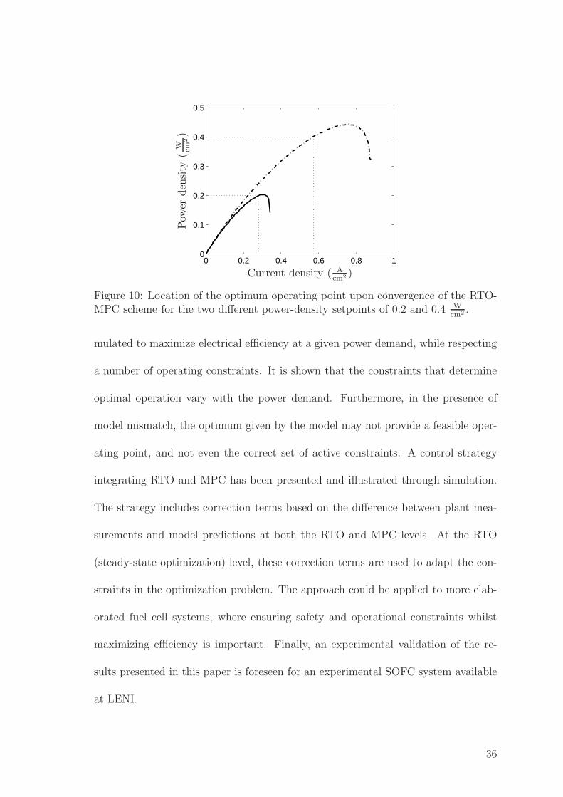
The power density vs. current density curves are shown in Figure 10. The location

of the optimal operating points obtained upon convergence of the RTO-MPC scheme

for the two different power setpoints are clearly indicated. In both cases, optimal

operation is on the left side of the maximum power density. The constraints on

34

0 10 20 30 40 50 60 70 80 90 1000.2

0.3

0.4

0.5

0.6

0.7

0 10 20 30 40 50 60 70 80 90 1000

0.005

0.01

0.015

0.02

0 10 20 30 40 50 60 70 80 90 1000.2

0.25

0.3

0.35

0.4

0 10 20 30 40 50 60 70 80 90 1000.1

0.2

0.3

0.4

0.5

0 10 20 30 40 50 60 70 80 90 1000.2

0.4

0.6

0.8

0 10 20 30 40 50 60 70 80 90 100

0.7

0.75

0.8

Time (min)Time (min)

FU

i(

Acm

2)

Pow

er(

W cm2)

η eff

Flo

wra

tes

(mol

s)

Uce

ll(V

)

nfuel,in

nair,in

Figure 9: Solid lines: Constraint adaptation with MPC for Case 2. Dashed lines:Power setpoint and constraint bounds. The three inputs are the flow rates nfuel,in

and nair,in, and the current I, which is considered proportional to the current densityi.

current density, cell potential and fuel utilization have prevented the operating point

from crossing to the right of the maximum power density. Note that the step response

model used by MPC was obtained on the left side of the maximum power density

and thus would become inadequate if the plant operation crosses to the right side.

Golbert and Lewin (2007) [2] have reported oscillatory behavior when the MPC

model and the plant are on different sides of the maximum power density.

6 Conclusions

This paper has considered the real-time optimization of a simple SOFC system. A

lumped dynamic model is used, which considers the electrochemical, energy and

mass balances taking place inside the cell. An optimization problem has been for-

35

0 0.2 0.4 0.6 0.8 10

0.1

0.2

0.3

0.4

0.5

Pow

erden

sity

(W cm

2)

Current density ( Acm2 )

Figure 10: Location of the optimum operating point upon convergence of the RTO-MPC scheme for the two different power-density setpoints of 0.2 and 0.4 W

cm2 .

mulated to maximize electrical efficiency at a given power demand, while respecting

a number of operating constraints. It is shown that the constraints that determine

optimal operation vary with the power demand. Furthermore, in the presence of

model mismatch, the optimum given by the model may not provide a feasible oper-

ating point, and not even the correct set of active constraints. A control strategy

integrating RTO and MPC has been presented and illustrated through simulation.

The strategy includes correction terms based on the difference between plant mea-

surements and model predictions at both the RTO and MPC levels. At the RTO

(steady-state optimization) level, these correction terms are used to adapt the con-

straints in the optimization problem. The approach could be applied to more elab-

orated fuel cell systems, where ensuring safety and operational constraints whilst

maximizing efficiency is important. Finally, an experimental validation of the re-

sults presented in this paper is foreseen for an experimental SOFC system available

at LENI.

36

References

[1] Zhang, X. W., Chan, S. H., Hob, H. K., Li, J., Li, G., and Feng, Z., 2008, “Non-

linear model predictive control based on the moving horizon state estimation

for the solid oxide fuel cell,” Int. J. Hydrogen Energy, 33, pp. 2355–2366.

[2] Golbert, J. and Lewin, D. R., 2007, “Model-based control of fuel cells (2):

Optimal efficiency,” J. Power Sources, 173, pp. 298–309.

[3] Aguiar, P., Adjiman, C., and Brandon, N., 2005, “Anode-supported

intermediate-temperature direct internal reforming solid oxide fuel cell II.

model-based dynamic performance and control,” J. Power Sources, 147, pp.

136–147.

[4] Golbert, J. and Lewin, D. R., 2004, “Model-based control of fuel cells: (1)

Regulatory control,” J. Power Sources, 135, pp. 135–151.

[5] Jurrado, F., 2006, “Predictive control of solid oxide fuel cells using fuzzy Ham-

merstein models,” J. Power Sources, 158, pp. 245–253.

[6] Wu, X.-J., Zhu, X.-J., Cao, G.-Y., and Tu, H.-Y., 2008, “Predictive control of

SOFC based on a GA-RBF neural network model,” J. Power Sources, 179, pp.

232–239.

[7] Mueller, F., Jabbaria, F., Gaynor, R., and Brouwer, J., 2007, “Novel solid oxide

fuel cell system controller for rapid load following,” J. Power Sources, 172, pp.

308–323.

37

[8] Marlin, T. E. and Hrymak, A. N., 1997, “Real-time operations optimization of

continuous processes,” AIChE Symposium Series - CPC-V, vol. 93, pp. 156–164.

[9] Qin, S. J. and Badgwell, T. A., 1997, “An overview of industrial model predic-

tive technology,” AIChE Symposium Series - CPC-V, vol. 93, pp. 232–256.

[10] Maarleveld, A. and Rijnsdorp, J. E., 1970, “Constraint control on distillation

columns,” Automatica, 6, pp. 51–58.

[11] Chachuat, B., Marchetti, A., and Bonvin, D., 2008, “Process optimization via

constraints adaptation,” J. Process Contr., 18, pp. 244–257.

[12] Forbes, J. F. and Marlin, T. E., 1994, “Model accuracy for economic optimizing

controllers: The bias update case,” Ind. Eng. Chem. Res., 33, pp. 1919–1929.

[13] Diethelm, S., van Herle, J., Wuillemin, Z., Nakajo, A., Autissier, N., and Mo-

linelli, M., 2008, “Impact of materials and design on solid oxide fuel cell stack

operation,” J. Fuel Cell Sci. Technol., 5(3), p. 31003.

[14] Wuillemin, Z., Autissier, N., Luong, M.-T., Van herle, J., and Favrat, D., 2008,

“Modeling and study of the influence of sealing on a solid oxide fuel cell,” J.

Fuel Cell Sci. Technol., 5, p. 011016.

[15] Nakajo, A., Wuillemin, Z., Van herle, J., and Favrat, D., 2009, “Simulation of

thermal stresses in anode-supported solid oxide fuel cell stacks. Part I: Proba-

bility of failure of the cells,” J. Power Sources, In press.

[16] Lienhard IV, J. H. and Lienhard V, J. H., 2003, A Heat Transfer Textbook,

Phlogiston Press, 3rd ed.

38

[17] Chan, S. H., Khor, K. A., and Xia, Z. T., 2001, “A complete polarization

model of a solid oxide fuel cell and its sensitivity to change of cell component

thickness,” J. Power Sources, 93, pp. 130–140.

[18] Park, J.-H. and Blumenthal, R. N., 1989, “Electronic transport in 8 mole per-

cent. Y2.O3.ZrO2,” J. Electrochem. Soc., 136, pp. 2867–2876.

[19] Larrain, D., Van herle, J., and Favrat, D., 2006, “Simulation of SOFC stack

and repeat elements including interconnect degradation and anode reoxidation

risk,” J. Power Sources, 161, pp. 392–403.

[20] Garcia, C. E. and Morari, M., 1984, “Optimal operation of integrated processing

systems. Part II: Closed-loop on-line optimizing control,” AIChE J., 30(2), pp.

226–234.

[21] Maciejowski, J. M., 2002, Predictive Control with Constraints, Prentice Hall,

New Jersey.

[22] Scokaert, P. O. M. and Rawlings, J. B., 1999, “Feasibility issues in linear model

predictive control,” AIChE J., 45(8), pp. 1649–1659.

[23] Marchetti, A., Chachuat, B., and Bonvin, D., 2008, “Real-time optimization

via adaptation and control of the constraints,” 18th European Symposium on

Computer Aided Process Engineering, ESCAPE 18, Lyon, France.

39