IEEE TRANSACTION ON IMAGE PROCESSING 1 Real-time Object Tracking via Online Discriminative Feature Selection Kaihua Zhang, Lei Zhang, and Ming-Hsuan Yang Abstract Most tracking-by-detection algorithms train discriminative classifiers to separate target objects from their surrounding background. In this setting, noisy samples are likely to be included when they are not properly sampled, thereby causing visual drift. The multiple instance learning (MIL) learning paradigm has been recently applied to alleviate this problem. However, important prior information of instance labels and the most correct positive instance (i.e., the tracking result in the current frame) can be exploited using a novel formulation much simpler than an MIL approach. In this paper, we show that integrating such prior information into a supervised learning algorithm can handle visual drift more effectively and efficiently than the existing MIL tracker. We present an online discriminative feature selection algorithm which optimizes the objective function in the steepest ascent direction with respect to the positive samples while in the steepest descent direction with respect to the negative ones. Therefore, the trained classifier directly couples its score with the importance of samples, leading to a more robust and efficient tracker. Numerous experimental evaluations with state-of-the-art algorithms on challenging sequences demonstrate the merits of the proposed algorithm. Index Terms Object tracking, multiple instance learning, supervised learning, online boosting. Kaihua Zhang and Lei Zhang are with the Department of Computing, the Hong Kong Polytechnic University, Hong Kong. E-mail: [email protected], [email protected]. Ming-Hsuan Yang is with Electrical Engineering and Computer Science, University of California, Merced, CA, 95344. E-mail: [email protected]. November 28, 2013 DRAFT

Welcome message from author
This document is posted to help you gain knowledge. Please leave a comment to let me know what you think about it! Share it to your friends and learn new things together.
Transcript
IEEE TRANSACTION ON IMAGE PROCESSING 1
Real-time Object Tracking via
Online Discriminative Feature Selection
Kaihua Zhang, Lei Zhang, and Ming-Hsuan Yang
Abstract
Most tracking-by-detection algorithms train discriminative classifiers to separate target objects from
their surrounding background. In this setting, noisy samples are likely to be included when they are not
properly sampled, thereby causing visual drift. The multiple instance learning (MIL) learning paradigm
has been recently applied to alleviate this problem. However, important prior information of instance
labels and the most correct positive instance (i.e., the tracking result in the current frame) can be
exploited using a novel formulation much simpler than an MIL approach. In this paper, we show that
integrating such prior information into a supervised learning algorithm can handle visual drift more
effectively and efficiently than the existing MIL tracker. We present an online discriminative feature
selection algorithm which optimizes the objective function in the steepest ascent direction with respect to
the positive samples while in the steepest descent direction with respect to the negative ones. Therefore,
the trained classifier directly couples its score with the importance of samples, leading to a more robust
and efficient tracker. Numerous experimental evaluations with state-of-the-art algorithms on challenging
sequences demonstrate the merits of the proposed algorithm.
Index Terms
Object tracking, multiple instance learning, supervised learning, online boosting.
Kaihua Zhang and Lei Zhang are with the Department of Computing, the Hong Kong Polytechnic University, Hong Kong.
E-mail: [email protected], [email protected].
Ming-Hsuan Yang is with Electrical Engineering and Computer Science, University of California, Merced, CA, 95344.
E-mail: [email protected].
November 28, 2013 DRAFT
IEEE TRANSACTION ON IMAGE PROCESSING 2
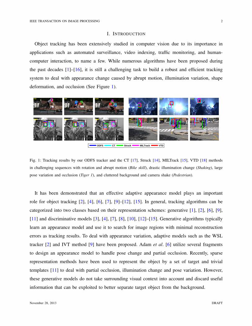
I. INTRODUCTION
Object tracking has been extensively studied in computer vision due to its importance in
applications such as automated surveillance, video indexing, traffic monitoring, and human-
computer interaction, to name a few. While numerous algorithms have been proposed during
the past decades [1]–[16], it is still a challenging task to build a robust and efficient tracking
system to deal with appearance change caused by abrupt motion, illumination variation, shape
deformation, and occlusion (See Figure 1).
#10 #60 #100 #10 #60 #320
#290 #312 #348 #52 #106 #139
#400
ODFS CT Struck MILTrack VTD
Fig. 1: Tracking results by our ODFS tracker and the CT [17], Struck [14], MILTrack [15], VTD [18] methods
in challenging sequences with rotation and abrupt motion (Bike skill), drastic illumination change (Shaking), large
pose variation and occlusion (Tiger 1), and cluttered background and camera shake (Pedestrian).
It has been demonstrated that an effective adaptive appearance model plays an important
role for object tracking [2], [4], [6], [7], [9]–[12], [15]. In general, tracking algorithms can be
categorized into two classes based on their representation schemes: generative [1], [2], [6], [9],
[11] and discriminative models [3], [4], [7], [8], [10], [12]–[15]. Generative algorithms typically
learn an appearance model and use it to search for image regions with minimal reconstruction
errors as tracking results. To deal with appearance variation, adaptive models such as the WSL
tracker [2] and IVT method [9] have been proposed. Adam et al. [6] utilize several fragments
to design an appearance model to handle pose change and partial occlusion. Recently, sparse
representation methods have been used to represent the object by a set of target and trivial
templates [11] to deal with partial occlusion, illumination change and pose variation. However,
these generative models do not take surrounding visual context into account and discard useful
information that can be exploited to better separate target object from the background.
November 28, 2013 DRAFT

IEEE TRANSACTION ON IMAGE PROCESSING 3
Discriminative models pose object tracking as a detection problem in which a classifier is
learned to separate the target object from its surrounding background within a local region [3].
Collins et al. [4] demonstrate that selecting discriminative features in an online manner improves
tracking performance. Boosting method has been used for object tracking [8] by combing weak
classifiers with pixel-based features within the target and background regions with the on-center
off-surround principle. Grabner et al. [7] propose an online boosting feature selection method
for object tracking. However, the above-mentioned discriminative algorithms [3], [4], [7], [8]
utilize only one positive sample (i.e., the tracking result in the current frame) and multiple
negative samples when updating the classifier. If the object location detected by the current
classifier is not precise, the positive sample will be noisy and result in a suboptimal classifier
update. Consequently, errors will be accumulated and cause tracking drift or failure [15]. To
alleviate the drifting problem, an online semi-supervised approach [10] is proposed to train the
classifier by only labeling the samples in the first frame while considering the samples in the
other frames as unlabeled. Recently, an efficient tracking algorithm [17] based on compres-
sive sensing theories [19], [20] is proposed. It demonstrates that the low dimensional features
randomly extracted from the high dimensional multiscale image features preserve the intrinsic
discriminative capability, thereby facilitating object tracking.
Several tracking algorithms have been developed within the multiple instance learning (MIL)
framework [13], [15], [21], [22] in order to handle location ambiguities of positive samples for
object tracking. In this paper, we demonstrate that it is unnecessary to use feature selection
method proposed in the MIL tracker [15], and instead an efficient feature selection method
based on optimization of the instance probability can be exploited for better performance.
Motivated by success of formulating the face detection problem with the multiple instance
learning framework [23], an online multiple instance learning method [15] is proposed to handle
the ambiguity problem of sample location by minimizing the bag likelihood loss function. We
note that in [13] the MILES model [24] is employed to select features in a supervised learning
manner for object tracking. However, this method runs at about 2 to 5 frames per second (FPS),
which is less efficient than the proposed algorithm (about 30 FPS). In addition, this method is
developed with the MIL framework and thus has similar drawbacks as the MILTrack method [15].
Recently, Hare et al. [14] show that the objectives for tracking and classification are not explicitly
coupled because the objective for tracking is to estimate the most correct object position while the
November 28, 2013 DRAFT

IEEE TRANSACTION ON IMAGE PROCESSING 4
-Training samples
+
Tracking resultConfidence mapTest samples
?
ζ
αβUpdate classifier
parameters ODFS
Frame (t+1)
γ
t★( )l x
t★
+1( )l x
Feature extraction
Object tracking procedure
Online classifier update procedure
Fig. 2: Main steps of the proposed algorithm.
objective for classification is to predict the instance labels. However, this issue is not addressed
in the existing discriminative tracking methods under the MIL framework [13], [15], [21], [22].
In this paper, we propose an efficient and robust tracking algorithm which addresses all the
above-mentioned issues. The key contributions of this work are summarized as follows.
1) We propose a simple and effective online discriminative feature selection (ODFS) approach
which directly couples the classifier score with the sample importance, thereby formulating
a more robust and efficient tracker than state-of-the-art algorithms [6], [7], [10]–[12], [14],
[15], [18] and 17 times faster than the MILTrack [15] method (both are implemented in
MATLAB).
2) We show that it is unnecessary to use bag likelihood loss functions for feature selection as
proposed in the MILTrack method. Instead, we can directly select features on the instance
level by using a supervised learning method which is more efficient and robust than the
MILTrack method. As all the instances, including the correct positive one, can be labeled
from the current classifier, they can be used for update via self-taught learning [25]. Here,
the most correct positive instance can be effectively used as the tracking result of the
current frame in a way similar to other discriminative models [3], [4], [7], [8].
II. PROBLEM FORMULATION
In this section, we present the algorithmic details and theoretical justifications of this work.
November 28, 2013 DRAFT

IEEE TRANSACTION ON IMAGE PROCESSING 5
Algorithm 1 ODFS TrackingInput: (t+1)-th video frame
1) Sample a set of image patches, Xγ = {x|||lt+1(x) − lt(x?)|| < γ} where lt(x?) is the
tracking location at the t-th frame, and extract the features {fk(x)}Kk=1 for each sample
2) Apply classifier hK in (2) to each feature vector and find the tracking location lt+1(x?)
where x? = arg maxx∈Xγ{c(x) = σ(hK(x))}
3) Sample two sets of image patches Xα = {x|||lt+1(x) − lt+1(x?)|| < α} and Xζ,β =
{x|ζ < ||lt+1(x)− lt+1(x?)|| < β} with α < ζ < β
4) Extract the features with these two sets of samples by the ODFS algorithm and update
the classifier parameters according to (5) and (6)
Output: Tracking location lt+1(x?) and classifier parameters
A. Tracking by Detection
The main steps of our tracking system are summarized in Algorithm 1. Figure 2 illustrates
the basic flow of our algorithm. Our discriminative appearance model is based a classifier hK(x)
which estimates the posterior probability
c(x) = P (y = 1|x) = σ(hK(x)), (1)
(i.e., confidence map function) where x is the sample represented by a feature vector f(x) =
(f1(x), . . . , fK(x))>, y ∈ {0, 1} is a binary variable which represents the sample label, and σ(·)
is a sigmoid function.
Given a classifier, the tracking by detection process is as follows. Let lt(x) ∈ R2 denote the lo-
cation of sample x at the t-th frame. We have the object location lt(x?) where we assume the cor-
responding sample is x?, and then we densely crop some patches Xα = {x |‖ lt(x)− lt(x?) ‖ <
α} within a search radius α centering at the current object location, and label them as positive
samples. Then, we randomly crop some patches from set Xζ,β = {x|ζ <‖ lt(x)− lt(x?) ‖< β}
where α < ζ < β, and label them as negative samples. We utilize these samples to update the
classifier hK . When the (t+1)-th frame arrives, we crop some patches Xγ = {x |‖ lt+1(x) −
lt(x?) ‖< γ} with a large radius γ surrounding the old object location lt(x?) in the (t+1)-
th frame. Next, we apply the updated classifier to these patches to find the patch with the
November 28, 2013 DRAFT

IEEE TRANSACTION ON IMAGE PROCESSING 6
maximum confidence i.e. x? = arg maxx(c(x)). The location lt+1(x?) is the new object location
in the (t+1)-th frame. Based on the newly detected object location, our tracking system repeats
the above-mentioned procedures.
B. Classifier Construction and Update
In this work, sample x is represented by a feature vector f(x) = (f1(x), . . . , fK(x))>, where
each feature is assumed to be independently distributed as MILTrack [15], and then the classifier
hK can be modeled by a naive Bayes classifier [26]
hK(x) = log
(∏Kk=1 p(fk(x)|y = 1)P (y = 1)∏Kk=1 p(fk(x)|y = 0)P (y = 0)
)=
K∑k=1
φk(x), (2)
where
φk(x) = log(p(fk(x)|y=1)p(fk(x)|y=0)
), (3)
is a weak classifier with equal prior, i.e., P (y = 1) = P (y = 0). Next, we have P (y = 1 |
x) = σ(hK(x)) (i.e., (1)), where the classifier hK is a linear function of weak classifiers and
σ(z) = 11+e−z
.
We use a set of Haar-like features fk [15] to represent samples. The conditional distributions
p(fk | y = 1) and p(fk | y = 0) in the classifier hK are assumed to be Gaussian distributed as
the MILTrack method [15] with four parameters (µ+k , σ
+k , µ
−k , σ
−k ) where
p(fk | y = 1) ∼ N (µ+k , σ
+k ), p(fk | y = 0) ∼ N (µ−k , σ
−k ). (4)
The parameters (µ+k , σ
+k , µ
−k , σ
−k ) in (4) are incrementally estimated as follows
µ+k ← ηµ+
k + (1− η)µ+, (5)
σ+k ←
√η(σ+
k )2 + (1− η)(σ+)2 + η(1− η)(µ+k − µ+)2, (6)
where η is the learning rate for update, σ+ =√
1N
∑N−1i=0|y=1(fk(xi)− µ+)2, and N is the number
of positive samples. In addition, µ+ = 1N
∑N−1i=0|y=1 fk(xi). We update µ−k and σ−k with similar
rules. The above-mentioned (5) and (6) can be easily deduced by maximum likelihood estimation
method [27] where η is a learning rate to moderate the balance between the former frames and
the current one.
It should be noted that our parameter update method is different from that of the MILTrack
method [15], and our update equations are derived based on maximum likelihood estimation.
November 28, 2013 DRAFT

IEEE TRANSACTION ON IMAGE PROCESSING 7
In Section III, we demonstrate that the importance and stability of this update method in
comparisons with [15].
For online object tracking, a feature pool with M > K features is maintained. As demon-
strated in [4], online selection of the discriminative features between object and background
can significantly improve the performance of tracking. Our objective is to estimate the sample
x? with the maximum confidence from (1) as x? = arg maxx(c(x)) with K selected features.
However, if we directly select K features from the pool of M features by using a brute force
method to maximize c(·), the computational complexity with CKM combinations is prohibitively
high (we set K = 15 and M = 150 in our experiments) for real-time object tracking. In the
following section, we propose an efficient online discriminative feature selection method which
is a sequential forward selection method [28] where the number of feature combinations is MK,
thereby facilitating real-time performance.
C. Online Discriminative Feature Selection
We first review the MILTrack method [15] as it is related to our work, and then introduce the
proposed ODFS algorithm.
1) Bag Likelihood with Noisy-OR Model: The instance probability of the MILTrack method
is modeled by Pij = σ(h(xij)) (i.e., (1)) where i indexes the bag and j indexes the instance in
the bag, and h =∑
k φk is a strong classifier. The weak classifier φk is computed by (3) and
the bag probability based on the Noisy-OR model is
Pi = 1−∏j
(1− Pij). (7)
The MILTrack method maintains a pool of M candidate weak classifiers, and selects K weak
classifiers from this pool in a greedy manner using the following criterion
φk = arg maxφ∈Φ
logL(hk−1 + φ), (8)
where Φ = {φi}Mi=1 is the weak classifier pool and each weak classifier is composed of a feature
(See (3)), L =∏
i Pyii (1 − Pi)1−yi is the bag likelihood function, and yi ∈ {0, 1} is a binary
label. The selected K weak classifiers construct the strong classifier as hK =∑K
k=1 φk. The
classifier hK is applied to the cropped patches in the new frame to determine the one with the
highest response as the most correct object location.
November 28, 2013 DRAFT

IEEE TRANSACTION ON IMAGE PROCESSING 8
We show that it is not necessary to use the bag likelihood function based on the Noisy-OR
model (8) for weak classifier selection, and we can select weak classifiers by directly optimizing
instance probability Pij = σ(hK(xij)) via a supervised learning method as both the most correct
positive instance (i.e., the tracking result in current frame) and the instance labels are assumed
to be known.
2) Principle of ODFS: In (1), the confidence map of a sample x being the target is computed,
and the object location is determined by the peak of the map, i.e., x? = arg maxx c(x). Providing
that the sample space is partitioned into two regions R+ = {x, y = 1} and R− = {x, y = 0},
we define a margin as the average confidence of samples in R+ minus the average confidence
of samples in R−:
Emargin =1
|R+|
∫x∈R+
c(x)dx− 1
|R−|
∫x∈R−
c(x)dx, (9)
where |R+| and |R−| are cardinalities of positive and negative sets, respectively.
In the training set, we assume the positive set R+ = {xi}N−1i=0 (where x0 is the tracking
result of the current frame) consists of N samples, and the negative set R− = {xi}N+L−1i=N is
composed of L samples (L ≈ N in our experiments). Therefore, replacing the integrals with the
corresponding sums and putting (2) and (1), we formulate (9) as
Emargin ≈1
N
(N−1∑i=0
σ( K∑k=1
φk(xi))−
N+L−1∑i=N
σ( K∑k=1
φk(xi))). (10)
Each sample xi is represented by a feature vector f(xi) = (f1(xi), . . . , fM(xi))>, a weak classifier
pool Φ = {φm}Mm=1 is maintained using (3). Our objective is to select a subset of weak classifiers
{φk}Kk=1 from the pool Φ which maximizes the average confidence of samples in R+ while
suppressing the average confidence of samples in R−. Therefore, we maximize the margin
function Emargin by
{φ1, . . . , φK} = arg max{φ1,...,φK}∈Φ
Emargin(φ1, . . . , φK). (11)
We use a greedy scheme to sequentially select one weak classifier from the pool Φ to maximize
November 28, 2013 DRAFT

IEEE TRANSACTION ON IMAGE PROCESSING 9
Emargin
φk = arg maxφ∈Φ
Emargin(φ1, . . . , φk−1, φ)
= arg maxφ∈Φ
N−1∑i=0
σ(hk−1(xi) + φ(xi))
−N+L−1∑i=N
σ(hk−1(xi) + φ(xi))
,
(12)
where hk−1(·) is a classifier constructed by a linear combination of the first (k-1) weak classifiers.
Note that it is difficult to find a closed form solution of the objective function in (12). Further-
more, although it is natural and easy to directly select φ that maximizes objective function in (12),
the selected φ is optimal only to the current samples {xi}N+L−1i=0 , which limits its generalization
capability for the extracted samples in the new frames. In the following section, we adopt an
approach similar to the approach used in the gradient boosting method [29] to solve (12) which
enhances the generalization capability for the selected weak classifiers.
The steepest descent direction of the objective function of (12) in the (N+L)-dimensional data
space at gk−1(x) is gk−1 = (gk−1(x0), . . . , gk−1(xN−1), −gk−1(xN), . . . ,−gk−1(xN+L−1))> where
gk−1(x) = −∂σ(hk−1(x))
∂hk−1
= −σ(hk−1(x))(1− σ(hk−1(x))), (13)
is the inverse gradient (i.e., the steepest descent direction) of the posterior probability function
σ(hk−1) with respect to hk−1. Since gk−1 is only defined at the points (x0, . . . , xN+L−1)>, its
generalization capability is limited. Friedman [29] proposes an approach to select φ that makes
φ = (φ(x0), . . . , φ(xN+L−1))> most parallel to gk−1 when minimizing our objective function in
(12). The selected weak classifier φ is most highly correlated with the gradient gk−1 over the data
distribution, thereby improving its generalization performance. In this work, we instead select
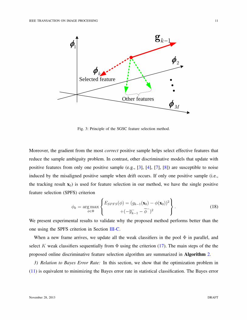
φ that is least parallel to gk−1 as we maximize the objective function (See Figure 3). Thus,
we choose the weak classifier φ with the following criterion which constrains the relationship
between Single Gradient and Single weak Classifier (SGSC) output for each sample:
φk = arg maxφ∈Φ
{ESGSC(φ) = ‖ gk−1 − φ ‖22}
= arg maxφ∈Φ
N−1∑i=0
(gk−1(xi)− φ(xi))2
+N+L−1∑i=N
(−gk−1(xi)− φ(xi))2
.
(14)
November 28, 2013 DRAFT

IEEE TRANSACTION ON IMAGE PROCESSING 10
However, the constraint between the selected weak classifier φ and the inverse gradient direction
gk−1 is still too strong in (14) because φ is limited to the a small pool Φ. In addition, both
the single gradient and the weak classifier output are easily affected by noise introduced by the
misaligned samples, which may lead to unstable results. To alleviate this problem, we relax the
constraint between φ and gk−1 with the Average Gradient and Average weak Classifier (AGAC)
criteria in a way similar to the regression tree method in [29]. That is, we take the average weak
classifier output for the positive and negative samples, and the average gradient direction instead
of each gradient direction for every sample,
φk = arg maxφ∈Φ
EAGAC(φ) = N(g+k−1 − φ
+)2
+L(−g−k−1 − φ−
)2
≈ arg max
φ∈Φ
((g+k−1 − φ
+)2 + (−g−k−1 − φ
−)2
),
(15)
where N is set approximately the same as L in our experiments. In addition, g+k−1 = 1
N
∑N−1i=0 gk−1(xi),
φ+
= 1N
∑N−1i=0 φ(xi), g−k−1 = 1
L
∑N+L−1i=N gk−1(xi), and φ
−= 1
L
∑N+L−1i=N φ(xi). It is easy to verify
ESGSC(φ) and EAGAC(φ) have the following relationship:
ESGSC(φ) = S2+ + S2
− + EAGAC(φ), (16)
where S2+ =
∑N−1i=0 (gk−1(xi)− φ(xi)− (g+
k−1 − φ+
))2 and S2− =
∑N+L−1i=N (−gk−1(xi)− φ(xi)−
(−g−k−1−φ−
))2. Therefore, (S2+ +S2
−)/N measures the variance of the pooled terms {gk−1(xi)−
φ(xi)}N−1i=0 and {−gk−1(xi)− φ(xi)}N+L−1
i=N . However, this pooled variance is easily affected by
noisy data or outliers. From (16), we have maxφ∈Φ EAGAC(φ) = maxφ∈Φ(ESGSC(φ)−(S2++S2
−)),
which means the selected weak classifier φ tends to maximize ESGSC while suppressing the
variance S2+ + S2
−, thereby leading to more stable results.
In our experiments, a small search radius (e.g., α = 4) is adopted to crop out the positive
samples in the neighborhood of the current object location, leading to the positive samples
with very similar appearances (See Figure 4). Therefore, we have g+k−1 = 1
N
∑N−1i=0 gk−1(xi) ≈
gk−1(x0). Replacing g+k−1 by gk−1(x0) in (15), the ODFS criterion becomes
φk = arg maxφ∈Φ
EODFS(φ) = (gk−1(x0)− φ+)2
+(−g−k−1 − φ−
)2
. (17)
It is worth noting that the average weak classifier output (i.e., φ+
in (17)) computed from
different positive samples alleviates the noise effects caused by some misaligned positive samples.
November 28, 2013 DRAFT
IEEE TRANSACTION ON IMAGE PROCESSING 11
1φ
Mφ
1k −g
kφ
Other features
2φ
Selected feature
Fig. 3: Principle of the SGSC feature selection method.
Moreover, the gradient from the most correct positive sample helps select effective features that
reduce the sample ambiguity problem. In contrast, other discriminative models that update with
positive features from only one positive sample (e.g., [3], [4], [7], [8]) are susceptible to noise
induced by the misaligned positive sample when drift occurs. If only one positive sample (i.e.,
the tracking result x0) is used for feature selection in our method, we have the single positive
feature selection (SPFS) criterion
φk = arg maxφ∈Φ
ESPFS(φ) = (gk−1(x0)− φ(x0))2
+(−g−k−1 − φ−
)2
. (18)
We present experimental results to validate why the proposed method performs better than the
one using the SPFS criterion in Section III-C.
When a new frame arrives, we update all the weak classifiers in the pool Φ in parallel, and
select K weak classifiers sequentially from Φ using the criterion (17). The main steps of the the
proposed online discriminative feature selection algorithm are summarized in Algorithm 2.
3) Relation to Bayes Error Rate: In this section, we show that the optimization problem in
(11) is equivalent to minimizing the Bayes error rate in statistical classification. The Bayes error
November 28, 2013 DRAFT

IEEE TRANSACTION ON IMAGE PROCESSING 12
Fig. 4: Illustration of cropping out positive samples with radius α = 4 pixels. The yellow rectangle denotes the
current tracking result and the white dash rectangles denote the positive samples.
rate [30] isPe = P (x ∈ R+, y = 0) + P (x ∈ R−, y = 1)
=
P (x ∈ R+|y = 0)P (y = 0)
+P (x ∈ R−|y = 1)P (y = 1)
=
∫R+ p(x ∈ R+|y = 0)P (y = 0)dx
+∫R− p(x ∈ R−|y = 1)P (y = 1)dx
,
(19)
where p(x|y) is the class conditional probability density function and P (y) describes the prior
probability. The posterior probability P (y|x) is computed by P (y|x) = p(x|y)P (y)/p(x), where
p(x) =∑1
j=0 p(x|y = j)P (y = j). Using (19), we have
Pe =
∫R+ P (y = 0|x ∈ R+)p(x ∈ R+)dx
+∫R− P (y = 1|x ∈ R−)p(x ∈ R−)dx
= −
∫ R+(P (y = 1|x ∈ R+)− 1)p(x ∈ R+)dx
−∫R− P (y = 1|x ∈ R−)p(x ∈ R−)dx
.
(20)
In our experiments, the samples in each set Rs, s = {+,−} are generated with equal probability,
i.e, p(x ∈ Rs) = 1|Rs| , where |Rs| is the cardinality of set Rs. Thus, we have
Pe = 1− Emargin, (21)
November 28, 2013 DRAFT

IEEE TRANSACTION ON IMAGE PROCESSING 13
Algorithm 2 Online Discriminative Feature Selection
Input: Dataset {xi, yi}N+L−1i=0 where yi ∈ {0, 1}.
1: Update weak classifier pool Φ = {φm}Mm=1 with data {xi, yi}N+L−1i=0 .
2: Update the average weak classifier outputs φ+
m and φ−m,m = 1, . . . ,M , in (15), respectively.
3: Initialize h0(xi) = 0.
4: for k = 1 to K do
5: Update gk−1(xi) by (13).
6: for m = 1 to M do
7: Em = (gk−1(x0)− φ+
m)2 + (−g−k−1 − φ−m)2.
8: end for
9: m? = arg maxm(Em).
10: φk ← φm? .
11: hk(xi)←∑k
j=1 φj(xi).
12: hk(xi)← hk(xi)/∑k
j=1 |φj(xi)| (Normalization).
13: end for
Output: Strong classifier hK(x) =∑K
k=1 φk(x) and confidence map function P (y = 1|x) =
σ(hK(x)).
where Emargin is our objective function (9). That is, maximizing the proposed objective function
Emargin is equivalent to minimizing the Bayes error rate Pe.
4) Discussion: We discuss the merits of the proposed algorithm with comparisons to the
MILTrack method and related work.
A. Assumption regarding the most positive sample. We assume the most correct positive sample
is the tracking result in the current frame. This has been widely used in discriminative models
with one positive sample [4], [7], [8]. Furthermore, most generative models [6], [9] assume the
tracking result in the current frame is the correct object representation which can also be seen
as the most positive sample. In fact, it is not possible for online algorithms to ensure a tracking
result is completely free of drift in the current frame (i.e., the classic problems in online learning,
semi-supervised learning, and self-taught learning). However, the average weak classifier output
November 28, 2013 DRAFT

IEEE TRANSACTION ON IMAGE PROCESSING 14
in our objective function of (17) can alleviate the noise effect caused by misaligned samples.
Moreover, our classifier couples its score with the importance of samples that can alleviate the
drift problem. Thus, we can alleviate this problem by considering the tracking result in the
current frame as the most correct positive sample.
B. Sample ambiguity problem. While the findings by Babenko et al. [15] demonstrate that the
location ambiguity problem can be alleviated with the online multiple instance learning approach,
the tracking results may still not be stable in some challenging tracking tasks [15]. This can be
explained by several factors. First, the Noisy-OR model used by MILTrack does not explicitly
treat the positive samples discriminatively, and instead selects less effective features. Second,
the classifier is only trained by the binary labels without considering the importance of each
sample. Thus, the maximum classifier score may not correspond to the most correct positive
sample, and a similar observation is recently stated by Hare et al. [14]. In our algorithm, the
feature selection criterion (i.e., (17)) explicitly relates the classifier score with the importance of
the samples. Therefore, the ambiguity problem can be better dealt with by the proposed method.
C. Sparse and discriminative feature selection. We examine Step 12 of Algorithm 2 in greater
detail. If we denote φj = wjψj , where ψj = sign(φj) can be seen as a binary weak classifier
whose output is only 1 or −1, and wj = |φj| is the weight of the binary weak classifier whose
range is [0,+∞) (refer to (3)). Therefore, the normalized equation in Step 12 can be rewritten
as hk ←∑k
i=1(ψiwi/∑k
j=1 |wj|), and we restrict hk to be the convex combination of elements
from the binary weak classifier set {ψi, i = 1, . . . , k}. This normalization procedure is critical
because it avoids the potential overfitting problem caused by arbitrary linear combination of
elements of the binary weak classifier set. In fact a similar problem also exists in the AnyBoost
algorithm [31]. We choose an `1 norm normalization method which helps to sparsely select the
most discriminative features. In our experiments, we only need to select 15 (K = 15) features
from a feature pool with 150 (M = 150) features, which is computationally more efficient than
the boosting feature selection techniques [7], [15] that select 50 (K = 50) features out of a pool
of 250 (M = 250) features in the experiments.
D. Advantages of ODFS over MILTrack. First, our ODFS method only needs to update the
gradient of the classifier once after selecting a feature, and this is much more efficient than
November 28, 2013 DRAFT
IEEE TRANSACTION ON IMAGE PROCESSING 15
the MILTrack method because all instance and bag probabilities must be updated M times
after selecting a weak classifier. Second, the ODFS method directly couples its classifier score
with the importance of the samples while the MILTrack algorithm does not. Thus the ODFS
method is able to select the most effective features related to the most correct positive instance.
This enables our tracker to better handle the drift problem than the MILTrack algorithm [15],
especially in case of drastic illumination change or heavy occlusion.
E. Differences with other online feature selection trackers. Online feature selection techniques
have been widely studied in object tracking [4], [7], [32]–[37]. In [36], Wang et al. use particle
filter method to select a set of Haar-like features to construct a binary classifier. Grabner et
al. [7] propose an online boosting algorithm to select Haar-like, HOG and LBP features. Liu
and Yu [37] propose a gradient-based online boosting algorithm to update a fixed number of HOG
features. The proposed ODFS algorithm is different from the aforementioned trackers. First, all
of the abovementioned trackers use only one target sample (i.e., the current tracking result) to
extract features. Thus, these features are easily affected by noise introduced by misaligned target
sample when tracking drift occurs. However, the proposed ODFS method suppresses noise by
averaging the outputs of the weak classifiers from all positive samples (See (17)). Second, the
final strong classifier in [7], [36], [37] generates only binary labels of samples (i.e., foreground
object or not). However, this is not explicitly coupled to the objective of tracking which is to
predict the object location [14]. The proposed ODFS algorithm selects features that maximize
the confidences of target samples while suppressing the confidences of background samples,
which is consistent with the objective of tracking.
The proposed algorithm is different from the method proposed by Liu and Yu [37] in another
two aspects. First, the algorithm by Liu and Yu does not select a small number of features
from a feature pool but uses all the features in the pool to construct a binary strong classifier. In
contrast, the proposed method selects a small number of features from a feature pool to construct
a confidence map. Second, the objective of [37] is to minimize the weighted least square error
between the estimated feature response and the true label whereas the objective of this work is
to maximize the margin between the average confidences of positive samples and negative ones
based on (9).
November 28, 2013 DRAFT
IEEE TRANSACTION ON IMAGE PROCESSING 16
−0.49443
0.6656−0.73772
−0.727480.097993
0.85336
−0.54569
0.018412
0.54176
−5 0 5
x 104
0
0.02
0.04
0.06
0.08
−5 −4 −3 −2 −1 0
x 105
0
0.02
0.04
0.06
0.08
0.1
0.12
0 0.5 1 1.5 2
x 105
0
0.01
0.02
0.03
0.04
0.05
0.06
0.07
0.08
0.09
Fig. 5: Probability distributions of three differently selected features that are linearly combined with two, three, four
rectangle features, respectively. The yellow numbers denote the corresponding weights. The red stair represents the
histogram of positive samples while the blue stair represents the histogram of negative samples. The red and blue
lines denote the corresponding distribution estimations by our incremental update method.
III. EXPERIMENTS
We use the same generalized Haar-like features as [15], which can be efficiently computed
using the integral image. Each feature fk is a Haar-like feature computed by the sum of weighted
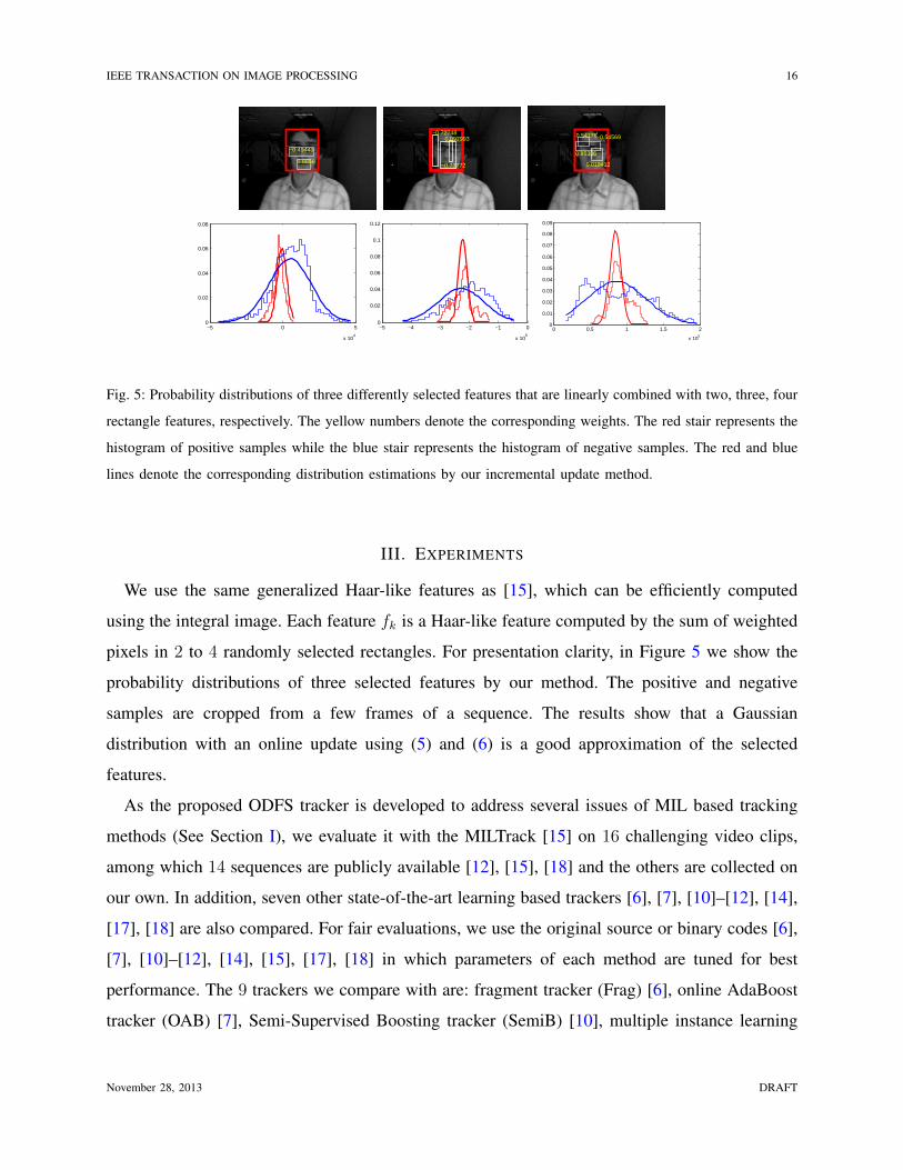
pixels in 2 to 4 randomly selected rectangles. For presentation clarity, in Figure 5 we show the
probability distributions of three selected features by our method. The positive and negative
samples are cropped from a few frames of a sequence. The results show that a Gaussian
distribution with an online update using (5) and (6) is a good approximation of the selected
features.
As the proposed ODFS tracker is developed to address several issues of MIL based tracking
methods (See Section I), we evaluate it with the MILTrack [15] on 16 challenging video clips,
among which 14 sequences are publicly available [12], [15], [18] and the others are collected on
our own. In addition, seven other state-of-the-art learning based trackers [6], [7], [10]–[12], [14],
[17], [18] are also compared. For fair evaluations, we use the original source or binary codes [6],
[7], [10]–[12], [14], [15], [17], [18] in which parameters of each method are tuned for best
performance. The 9 trackers we compare with are: fragment tracker (Frag) [6], online AdaBoost
tracker (OAB) [7], Semi-Supervised Boosting tracker (SemiB) [10], multiple instance learning
November 28, 2013 DRAFT
IEEE TRANSACTION ON IMAGE PROCESSING 17
tracker (MILTrack) [15], Tracking-Learning-Detection (TLD) method [12], Struck method [14],
`1-tracker [11], visual tracking decomposition (VTD) method [18] and compressive tracker
(CT) [17]. We fix the parameters of the proposed algorithm for all experiments to demonstrate
its robustness and stability. Since all the evaluated algorithms involve some random sampling
except [6], we repeat the experiments 10 times on each sequence, and present the averaged
results. Implemented in MATLAB, our tracker runs at 30 frames per second (FPS) on a Pentium
Dual-Core 2.10 GHz CPU with 1.95 GB RAM. Our source codes and videos are available at
http://www4.comp.polyu.edu.hk/∼cslzhang/ODFS/ODFS.htm.
0 200 400 6000
10
20
30
40
50
Frame#
Pos
ition
Err
or(p
ixel
)
David
ODFSCTStruckMILTrackVTD
0 200 400 6000
50
100
150
Frame#
Pos
ition
Err
or(p
ixel
)
Twinings
ODFSCTStruckMILTrackVTD
0 50 1000
50
100
150
Frame#
Pos
ition
Err
or(p
ixel
)
Kitesurf
ODFSCTStruckMILTrackVTD
0 200 400 600 8000
100
200
300
Frame#
Pos
ition
Err
or(p
ixel
)
Panda
ODFSCTStruckMILTrackVTD
0 500 10000
50
100
150
200
Frame#
Pos
ition
Err
or(p
ixel
)
Occluded face 2
ODFSCTStruckMILTrackVTD
0 100 200 300 4000
50
100
150
Frame#
Pos
ition
Err
or(p
ixel
)
Tiger 1
ODFSCTStruckMILTrackVTD
0 100 200 300 4000
50
100
150
Frame#
Pos
ition
Err
or(p
ixel
)
Tiger 2
ODFSCTStruckMILTrackVTD
0 100 200 300 4000
50
100
150
200
250
Frame#P
ositi
on E
rror
(pix
el)
Soccer
ODFSCTStruckMILTrackVTD
0 20 40 60 800
50
100
150
200
Frame#
Pos
ition
Err
or(p
ixel
)
Animal
ODFSCTStruckMILTrackVTD
0 50 100 1500
100
200
300
Frame#
Pos
ition
Err
or(p
ixel
)
Bike skill
ODFSCTStruckMILTrackVTD
0 100 200 300 4000
50
100
150
200
Frame#
Pos
ition
Err
or(p
ixel
)
Jumping
ODFSCTStruckMILTrackVTD
0 100 200 300 4000
50
100
150
200
Frame#
Pos
ition
Err
or(p
ixel
)
Coupon book
ODFSCTStruckMILTrackVTD
0 100 200 300 4000
50
100
150
Frame#
Pos
ition
Err
or(p
ixel
)
Cliff bar
ODFSCTStruckMILTrackVTD
0 100 200 300 4000
20
40
60
80
100
Frame#
Pos
ition
Err
or(p
ixel
)
Football
ODFSCTStruckMILTrackVTD
0 50 100 1500
50
100
150
200
Frame#
Pos
ition
Err
or(p
ixel
)
Pedestrian
ODFSCTStruckMILTrackVTD
0 100 200 300 4000
20
40
60
80
Frame#
Pos
ition
Err
or(p
ixel
)
Shaking
ODFSCTStruckMILTrackVTD
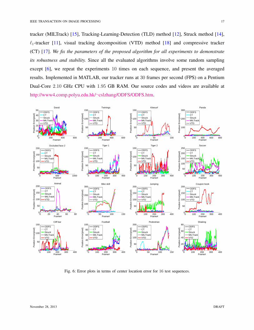
Fig. 6: Error plots in terms of center location error for 16 test sequences.
November 28, 2013 DRAFT

IEEE TRANSACTION ON IMAGE PROCESSING 18
A. Experimental Setup
We use a radius (α) of 4 pixels for cropping the similar positive samples in each frame
and generate 45 positive samples. A large α can make positive samples much different which
may add more noise but a small α generates a small number of positive samples which are
insufficient to avoid noise. The inner and outer radii for the set Xζ,β that generates negative
samples are set as ζ = d2αe = 8 and β = d1.5γe = 38, respectively. Note that we set the inner
radius ζ larger than the radius α to reduce the overlaps with the positive samples, which can
reduce the ambiguity between the positive and negative samples. Then, we randomly select a
set of 40 negative samples from the set Xζ,β which is fewer than that of the MILTrack method
(where 65 negative examples are used). Moreover, we do not need to utilize many samples to
initialize the classifier whereas the MILTrack method uses 1000 negative patches. The radius for
searching the new object location in the next frame is set as γ = 25 that is enough to take into
account all possible object locations because the object motion between two consecutive frames
is often smooth, and 2000 samples are drawn, which is the same as the MILTrack method [15].
Therefore, this procedure is time-consuming if we use more features in the classifier design. Our
ODFS tracker selects 15 features for classifier construction which is much more efficient than
the MILTrack method that sets K = 50. The number of candidate features M in the feature pool
is set to 150, which is fewer than that of the MILTrack method (M = 250). We note that we also
evaluate with the parameter settings K = 15,M = 150 in the MILTrack method but find it does
not perform well for most experiments. The learning parameter can be set as η = 0.80 ∼ 0.95.
A smaller learning rate can make the tracker quickly adapts to the fast appearance changes and
a larger learning rate can reduce the likelihood that the tracker drifts off the target. Good results
can be achieved by fixing η = 0.93 in our experiments.
B. Experimental Results
All of the test sequences consist of gray-level images and the ground truth object locations are
obtained by manual labels at each frame. We use the center location error in pixels as an index
to quantitatively compare 10 object tracking algorithms. In addition, we use the success rate to
evaluate the tracking results [14]. This criterion is used in the PASCAL VOC challenge [38]
and the score is defined as score = area(G⋂T )
area(G⋃T )
, where G is the ground truth bounding box
and T is the tracked bounding box. If score is larger than 0.5 in one frame, then the result
November 28, 2013 DRAFT
IEEE TRANSACTION ON IMAGE PROCESSING 19
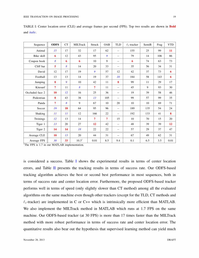
TABLE I: Center location error (CLE) and average frames per second (FPS). Top two results are shown in Bold
and italic.
Sequence ODFS CT MILTrack Struck OAB TLD `1-tracker SemiB Frag VTD
Animal 15 17 32 17 62 − 155 25 99 11
Bike skill 6 12 43 95 9 − 79 14 106 86
Coupon book 8 6 6 10 9 − 6 74 63 73
Cliff bar 5 8 14 20 33 − 35 56 34 31
David 12 17 19 9 57 12 42 37 73 6
Football 13 13 14 19 37 10 184 58 143 6
Jumping 8 9 10 42 11 8 99 11 29 17
Kitesurf 7 11 8 7 11 − 45 9 93 30
Occluded face 2 10 12 16 25 36 − 19 39 58 46
Pedestrian 8 43 38 13 105 − 99 57 99 35
Panda 7 8 9 67 10 20 10 10 69 71
Soccer 19 18 64 95 96 − 189 135 54 24
Shaking 11 11 12 166 22 − 192 133 41 8
Twinings 12 13 14 7 7 15 10 70 15 20
Tiger 1 13 20 27 12 42 − 48 39 39 12
Tiger 2 14 14 18 22 22 − 57 29 37 47
Average CLE 10 13 20 44 31 − 67 49 62 31
Average FPS 30 33 10.31 0.01 8.5 9.4 0.1 6.5 3.5 0.011The FPS is 1.7 in our MATLAB implementation.
is considered a success. Table I shows the experimental results in terms of center location
errors, and Table II presents the tracking results in terms of success rate. Our ODFS-based
tracking algorithm achieves the best or second best performance in most sequences, both in
terms of success rate and center location error. Furthermore, the proposed ODFS-based tracker
performs well in terms of speed (only slightly slower than CT method) among all the evaluated
algorithms on the same machine even though other trackers (except for the TLD, CT methods and
`1-tracker) are implemented in C or C++ which is intrinsically more efficient than MATLAB.
We also implement the MILTrack method in MATLAB which runs at 1.7 FPS on the same
machine. Our ODFS-based tracker (at 30 FPS) is more than 17 times faster than the MILTrack
method with more robust performance in terms of success rate and center location error. The
quantitative results also bear out the hypothesis that supervised learning method can yield much
November 28, 2013 DRAFT
IEEE TRANSACTION ON IMAGE PROCESSING 20
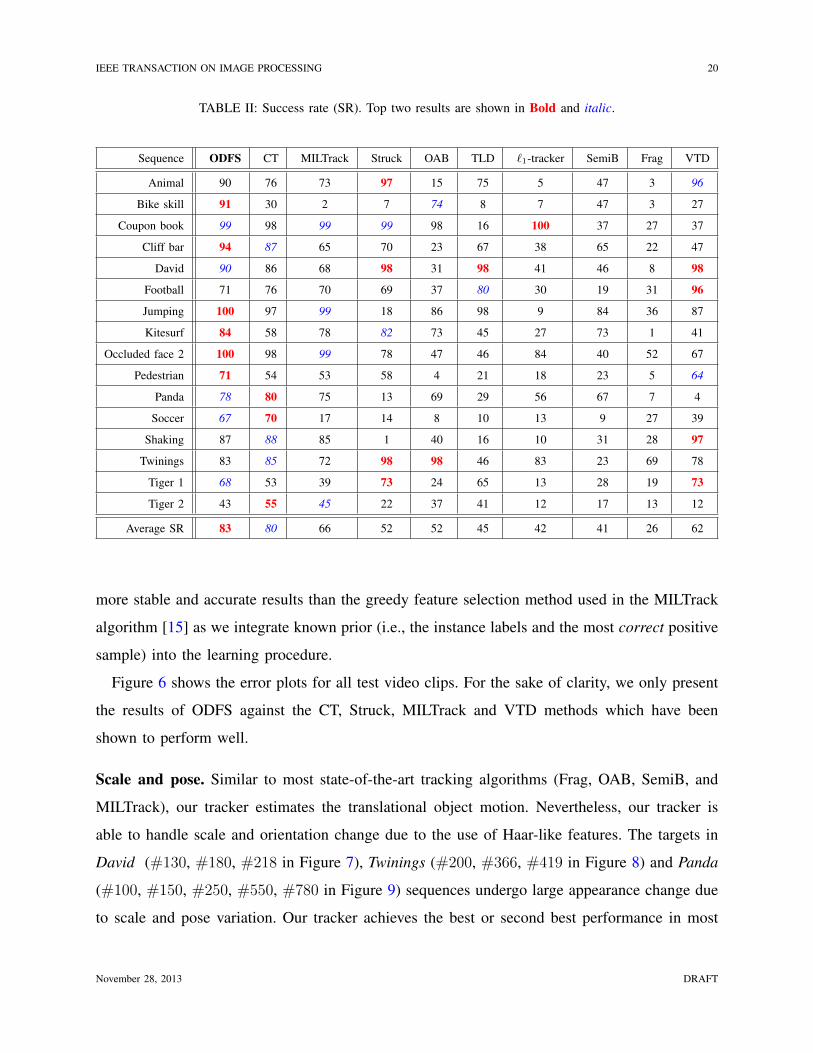
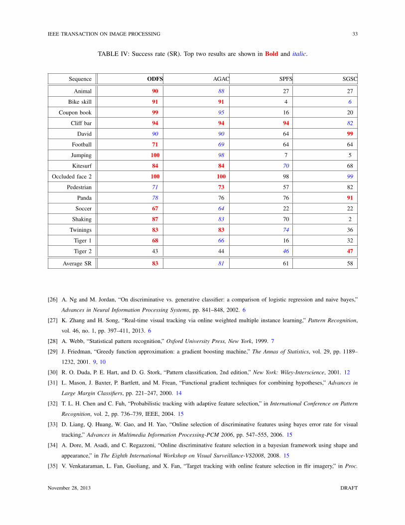
TABLE II: Success rate (SR). Top two results are shown in Bold and italic.
Sequence ODFS CT MILTrack Struck OAB TLD `1-tracker SemiB Frag VTD
Animal 90 76 73 97 15 75 5 47 3 96
Bike skill 91 30 2 7 74 8 7 47 3 27
Coupon book 99 98 99 99 98 16 100 37 27 37
Cliff bar 94 87 65 70 23 67 38 65 22 47
David 90 86 68 98 31 98 41 46 8 98
Football 71 76 70 69 37 80 30 19 31 96
Jumping 100 97 99 18 86 98 9 84 36 87
Kitesurf 84 58 78 82 73 45 27 73 1 41
Occluded face 2 100 98 99 78 47 46 84 40 52 67
Pedestrian 71 54 53 58 4 21 18 23 5 64
Panda 78 80 75 13 69 29 56 67 7 4
Soccer 67 70 17 14 8 10 13 9 27 39
Shaking 87 88 85 1 40 16 10 31 28 97
Twinings 83 85 72 98 98 46 83 23 69 78
Tiger 1 68 53 39 73 24 65 13 28 19 73
Tiger 2 43 55 45 22 37 41 12 17 13 12
Average SR 83 80 66 52 52 45 42 41 26 62
more stable and accurate results than the greedy feature selection method used in the MILTrack
algorithm [15] as we integrate known prior (i.e., the instance labels and the most correct positive
sample) into the learning procedure.
Figure 6 shows the error plots for all test video clips. For the sake of clarity, we only present
the results of ODFS against the CT, Struck, MILTrack and VTD methods which have been
shown to perform well.
Scale and pose. Similar to most state-of-the-art tracking algorithms (Frag, OAB, SemiB, and
MILTrack), our tracker estimates the translational object motion. Nevertheless, our tracker is
able to handle scale and orientation change due to the use of Haar-like features. The targets in
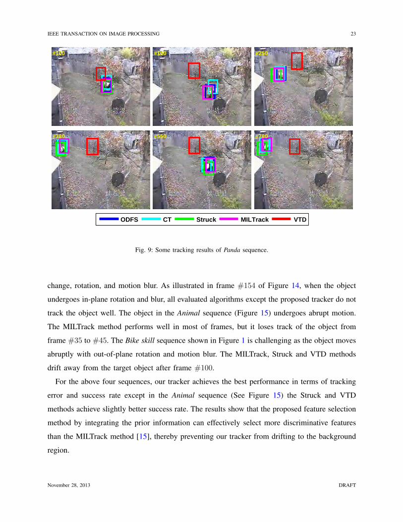
David (#130, #180, #218 in Figure 7), Twinings (#200, #366, #419 in Figure 8) and Panda
(#100, #150, #250, #550, #780 in Figure 9) sequences undergo large appearance change due
to scale and pose variation. Our tracker achieves the best or second best performance in most
November 28, 2013 DRAFT
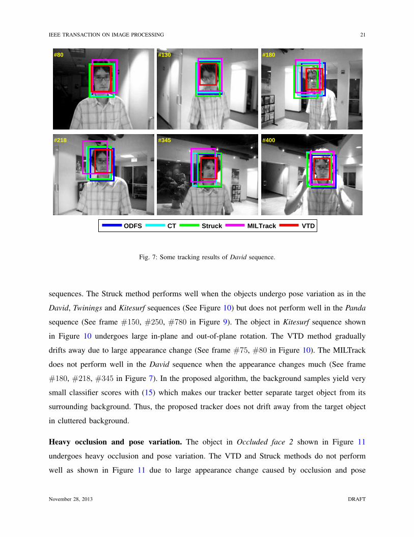
IEEE TRANSACTION ON IMAGE PROCESSING 21
#80 #130 #180
#218 #345 #400
#400
ODFS CT Struck MILTrack VTD
Fig. 7: Some tracking results of David sequence.
sequences. The Struck method performs well when the objects undergo pose variation as in the
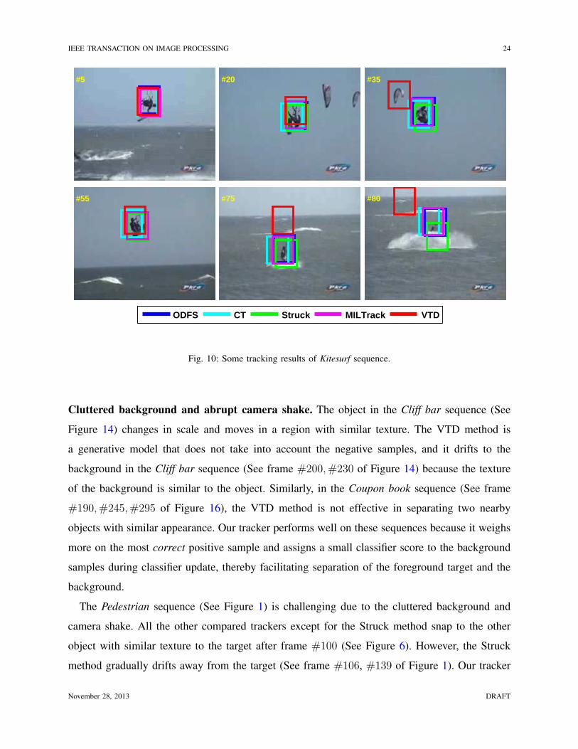
David, Twinings and Kitesurf sequences (See Figure 10) but does not perform well in the Panda
sequence (See frame #150, #250, #780 in Figure 9). The object in Kitesurf sequence shown
in Figure 10 undergoes large in-plane and out-of-plane rotation. The VTD method gradually
drifts away due to large appearance change (See frame #75, #80 in Figure 10). The MILTrack
does not perform well in the David sequence when the appearance changes much (See frame
#180, #218, #345 in Figure 7). In the proposed algorithm, the background samples yield very
small classifier scores with (15) which makes our tracker better separate target object from its
surrounding background. Thus, the proposed tracker does not drift away from the target object
in cluttered background.
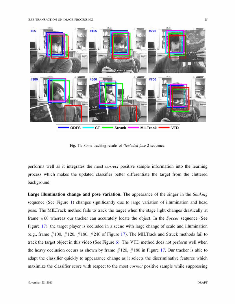
Heavy occlusion and pose variation. The object in Occluded face 2 shown in Figure 11
undergoes heavy occlusion and pose variation. The VTD and Struck methods do not perform
well as shown in Figure 11 due to large appearance change caused by occlusion and pose
November 28, 2013 DRAFT
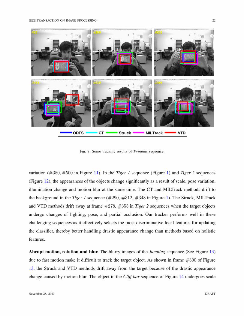
IEEE TRANSACTION ON IMAGE PROCESSING 22
#20 #100 #200
#366 #419 #466
#400
ODFS CT Struck MILTrack VTD
Fig. 8: Some tracking results of Twinings sequence.
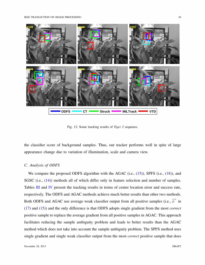
variation (#380,#500 in Figure 11). In the Tiger 1 sequence (Figure 1) and Tiger 2 sequences
(Figure 12), the appearances of the objects change significantly as a result of scale, pose variation,
illumination change and motion blur at the same time. The CT and MILTrack methods drift to
the background in the Tiger 1 sequence (#290, #312, #348 in Figure 1). The Struck, MILTrack
and VTD methods drift away at frame #278, #355 in Tiger 2 sequences when the target objects
undergo changes of lighting, pose, and partial occlusion. Our tracker performs well in these
challenging sequences as it effectively selects the most discriminative local features for updating
the classifier, thereby better handling drastic appearance change than methods based on holistic
features.
Abrupt motion, rotation and blur. The blurry images of the Jumping sequence (See Figure 13)
due to fast motion make it difficult to track the target object. As shown in frame #300 of Figure
13, the Struck and VTD methods drift away from the target because of the drastic appearance
change caused by motion blur. The object in the Cliff bar sequence of Figure 14 undergoes scale
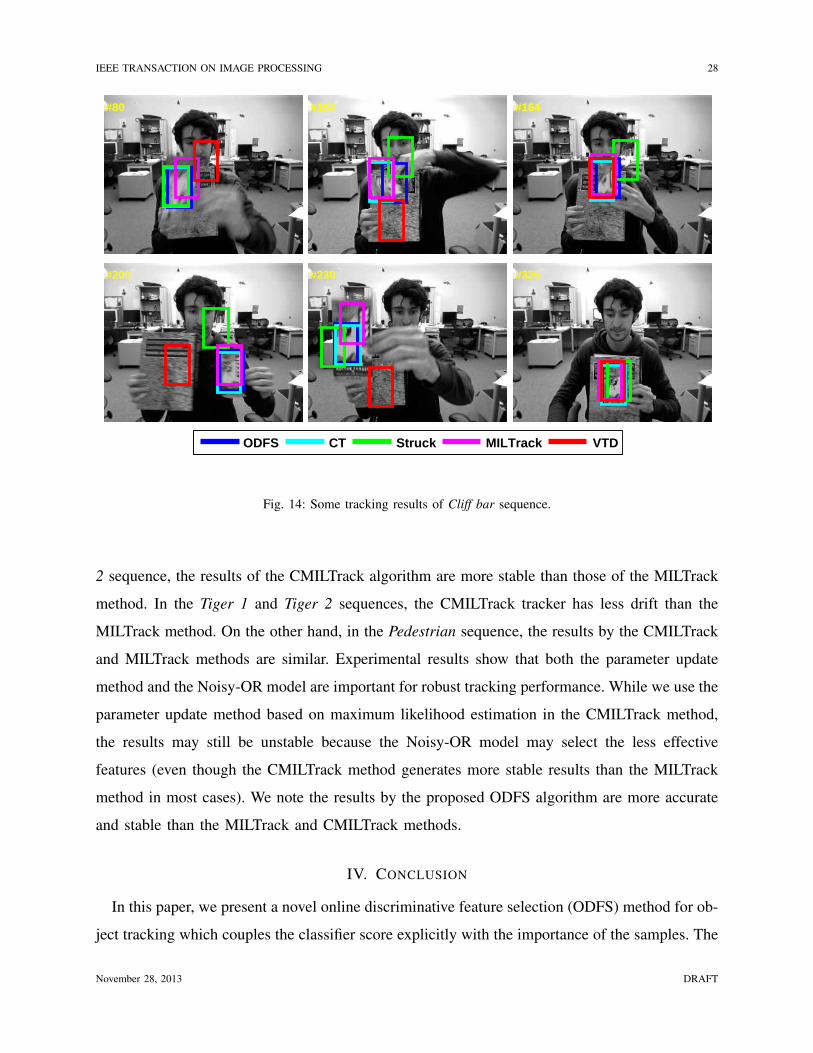
November 28, 2013 DRAFT
IEEE TRANSACTION ON IMAGE PROCESSING 23
#100 #150 #250
#380 #550 #780
#400
ODFS CT Struck MILTrack VTD
Fig. 9: Some tracking results of Panda sequence.
change, rotation, and motion blur. As illustrated in frame #154 of Figure 14, when the object
undergoes in-plane rotation and blur, all evaluated algorithms except the proposed tracker do not
track the object well. The object in the Animal sequence (Figure 15) undergoes abrupt motion.
The MILTrack method performs well in most of frames, but it loses track of the object from
frame #35 to #45. The Bike skill sequence shown in Figure 1 is challenging as the object moves
abruptly with out-of-plane rotation and motion blur. The MILTrack, Struck and VTD methods
drift away from the target object after frame #100.
For the above four sequences, our tracker achieves the best performance in terms of tracking
error and success rate except in the Animal sequence (See Figure 15) the Struck and VTD
methods achieve slightly better success rate. The results show that the proposed feature selection
method by integrating the prior information can effectively select more discriminative features
than the MILTrack method [15], thereby preventing our tracker from drifting to the background
region.
November 28, 2013 DRAFT
IEEE TRANSACTION ON IMAGE PROCESSING 24
#5 #20 #35
#55 #75 #80
#400
ODFS CT Struck MILTrack VTD
Fig. 10: Some tracking results of Kitesurf sequence.
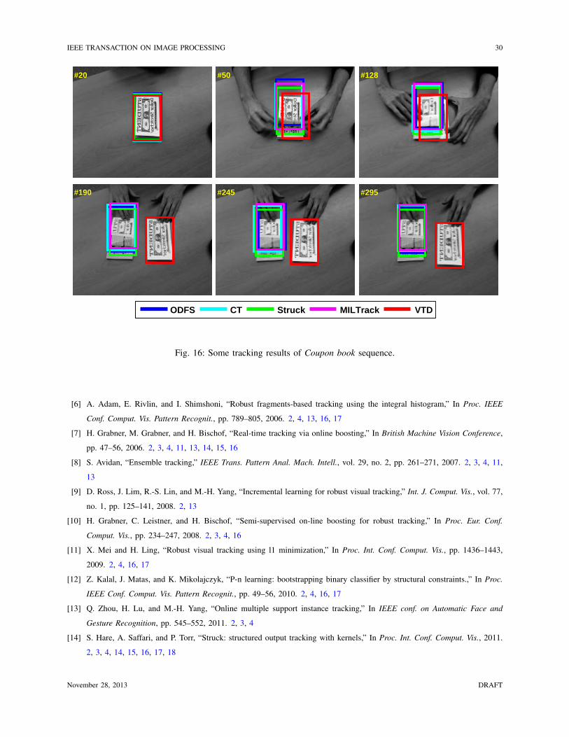
Cluttered background and abrupt camera shake. The object in the Cliff bar sequence (See
Figure 14) changes in scale and moves in a region with similar texture. The VTD method is
a generative model that does not take into account the negative samples, and it drifts to the
background in the Cliff bar sequence (See frame #200,#230 of Figure 14) because the texture
of the background is similar to the object. Similarly, in the Coupon book sequence (See frame
#190,#245,#295 of Figure 16), the VTD method is not effective in separating two nearby
objects with similar appearance. Our tracker performs well on these sequences because it weighs
more on the most correct positive sample and assigns a small classifier score to the background
samples during classifier update, thereby facilitating separation of the foreground target and the
background.
The Pedestrian sequence (See Figure 1) is challenging due to the cluttered background and
camera shake. All the other compared trackers except for the Struck method snap to the other
object with similar texture to the target after frame #100 (See Figure 6). However, the Struck
method gradually drifts away from the target (See frame #106, #139 of Figure 1). Our tracker
November 28, 2013 DRAFT
IEEE TRANSACTION ON IMAGE PROCESSING 25
#55 #155 #270
#380 #500 #700
#400
ODFS CT Struck MILTrack VTD
Fig. 11: Some tracking results of Occluded face 2 sequence.
performs well as it integrates the most correct positive sample information into the learning
process which makes the updated classifier better differentiate the target from the cluttered
background.
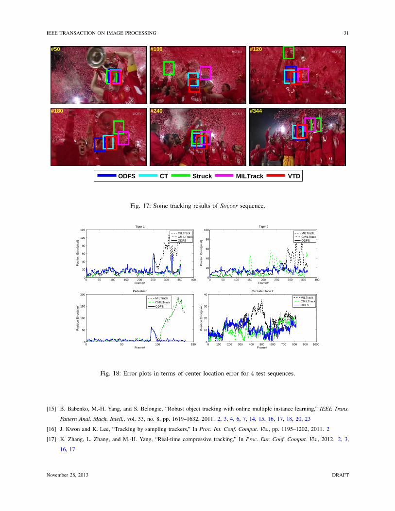
Large illumination change and pose variation. The appearance of the singer in the Shaking
sequence (See Figure 1) changes significantly due to large variation of illumination and head
pose. The MILTrack method fails to track the target when the stage light changes drastically at
frame #60 whereas our tracker can accurately locate the object. In the Soccer sequence (See
Figure 17), the target player is occluded in a scene with large change of scale and illumination
(e.g., frame #100, #120, #180, #240 of Figure 17). The MILTrack and Struck methods fail to
track the target object in this video (See Figure 6). The VTD method does not perform well when
the heavy occlusion occurs as shown by frame #120, #180 in Figure 17. Our tracker is able to
adapt the classifier quickly to appearance change as it selects the discriminative features which
maximize the classifier score with respect to the most correct positive sample while suppressing
November 28, 2013 DRAFT
IEEE TRANSACTION ON IMAGE PROCESSING 26
#108 #138 #257
#278 #330 #355
#400
ODFS CT Struck MILTrack VTD
Fig. 12: Some tracking results of Tiger 2 sequence.
the classifier score of background samples. Thus, our tracker performs well in spite of large
appearance change due to variation of illumination, scale and camera view.
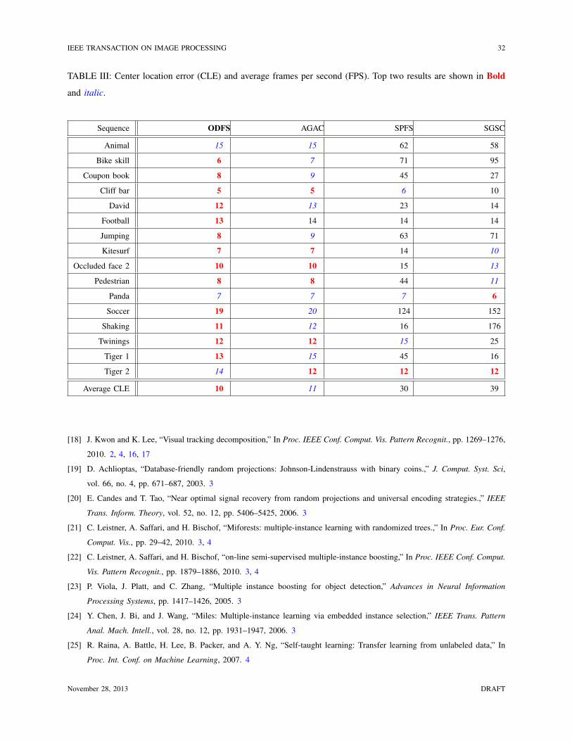
C. Analysis of ODFS
We compare the proposed ODFS algorithm with the AGAC (i.e., (15)), SPFS (i.e., (18)), and
SGSC (i.e., (14)) methods all of which differ only in feature selection and number of samples.
Tables III and IV present the tracking results in terms of center location error and success rate,
respectively. The ODFS and AGAC methods achieve much better results than other two methods.
Both ODFS and AGAC use average weak classifier output from all positive samples (i.e., φ+
in
(17) and (15)) and the only difference is that ODFS adopts single gradient from the most correct
positive sample to replace the average gradient from all positive samples in AGAC. This approach
facilitates reducing the sample ambiguity problem and leads to better results than the AGAC
method which does not take into account the sample ambiguity problem. The SPFS method uses
single gradient and single weak classifier output from the most correct positive sample that does
November 28, 2013 DRAFT

IEEE TRANSACTION ON IMAGE PROCESSING 27
#30 #100 #200
#250 #280 #300
#400
ODFS CT Struck MILTrack VTD
Fig. 13: Some tracking results of Jumping sequence.
not have the sample ambiguity problem. However, the noisy effect introduced by the misaligned
samples significantly affects its performance. The SGSC method does not work well because of
both noisy and sample ambiguity problems. Both the gradient from the most correct positive
sample and the average weak classifier output from all positive samples play important roles for
the performance of ODFS. The adopted gradient reduces the sample ambiguity problem while
the averaging process alleviates the noisy effect caused by some misaligned positive samples.
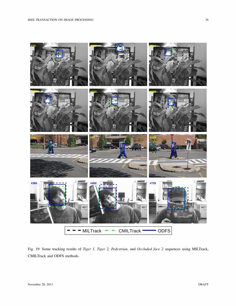
D. Online Update of Model Parameters
We implement our parameter update method in MATLAB with evaluation on 4 sequences, and
the MILTrack method using our parameter update method is referred as CMILTrack as illustrated
in Section . For fair comparisons, the only difference between the MATLAB implementations
of the MILTrack and CMILTrack methods is the parameter update module. We compare the
proposed ODFS, MILTrack and CMILTrack methods using four videos. Figure 18 shows the
error plots and some sampled results are shown in Figure 19. We note that in the Occluded face
November 28, 2013 DRAFT
IEEE TRANSACTION ON IMAGE PROCESSING 28
#80 #154 #164
#200 #230 #325
#400
ODFS CT Struck MILTrack VTD
Fig. 14: Some tracking results of Cliff bar sequence.
2 sequence, the results of the CMILTrack algorithm are more stable than those of the MILTrack
method. In the Tiger 1 and Tiger 2 sequences, the CMILTrack tracker has less drift than the
MILTrack method. On the other hand, in the Pedestrian sequence, the results by the CMILTrack
and MILTrack methods are similar. Experimental results show that both the parameter update
method and the Noisy-OR model are important for robust tracking performance. While we use the
parameter update method based on maximum likelihood estimation in the CMILTrack method,
the results may still be unstable because the Noisy-OR model may select the less effective
features (even though the CMILTrack method generates more stable results than the MILTrack
method in most cases). We note the results by the proposed ODFS algorithm are more accurate
and stable than the MILTrack and CMILTrack methods.
IV. CONCLUSION
In this paper, we present a novel online discriminative feature selection (ODFS) method for ob-
ject tracking which couples the classifier score explicitly with the importance of the samples. The
November 28, 2013 DRAFT

IEEE TRANSACTION ON IMAGE PROCESSING 29
#12 #25 #42
#56 #60 #71
#400
ODFS CT Struck MILTrack VTD
Fig. 15: Some tracking results of Animal sequence.
proposed ODFS method selects features which optimize the classifier objective function in the
steepest ascent direction with respect to the positive samples while in steepest descent direction
with respect to the negative ones. This leads to a more robust and efficient tracker without param-
eter tuning. Our tracking algorithm is easy to implement and achieves real-time performance with
MATLAB implementation on a Pentium dual-core machine. Experimental results on challenging
video sequences demonstrate that our tracker achieves favorable performance when compared
with several state-of-the-art algorithms.
REFERENCES
[1] M. Black and A. Jepson, “Eigentracking: Robust matching and tracking of articulated objects using a view-based
representation,” In Proc. Eur. Conf. Comput. Vis., pp. 329–342, 1996. 2
[2] A. Jepson, D. Fleet, and T. El-Maraghi, “Robust online appearance models for visual tracking,” IEEE Trans. Pattern Anal.
Mach. Intell., vol. 25, no. 10, pp. 1296–1311, 2003. 2
[3] S. Avidan, “Support vector tracking,” IEEE Trans. Pattern Anal. Mach. Intell., vol. 29, no. 8, pp. 1064–1072, 2004. 2, 3,
4, 11
[4] R. Collins, Y. Liu, and M. Leordeanu, “Online selection of discriminative tracking features,” IEEE Trans. Pattern Anal.
Mach. Intell., vol. 27, no. 10, pp. 1631–1643, 2005. 2, 3, 4, 7, 11, 13, 15
[5] M. Yang and Y. Wu, “Tracking non-stationary appearances and dynamic feature selection,” In Proc. IEEE Conf. Comput.
Vis. Pattern Recognit., pp. 1059–1066, 2005. 2
November 28, 2013 DRAFT
IEEE TRANSACTION ON IMAGE PROCESSING 30
#20 #50 #128
#190 #245 #295
#400
ODFS CT Struck MILTrack VTD
Fig. 16: Some tracking results of Coupon book sequence.
[6] A. Adam, E. Rivlin, and I. Shimshoni, “Robust fragments-based tracking using the integral histogram,” In Proc. IEEE
Conf. Comput. Vis. Pattern Recognit., pp. 789–805, 2006. 2, 4, 13, 16, 17
[7] H. Grabner, M. Grabner, and H. Bischof, “Real-time tracking via online boosting,” In British Machine Vision Conference,
pp. 47–56, 2006. 2, 3, 4, 11, 13, 14, 15, 16
[8] S. Avidan, “Ensemble tracking,” IEEE Trans. Pattern Anal. Mach. Intell., vol. 29, no. 2, pp. 261–271, 2007. 2, 3, 4, 11,
13
[9] D. Ross, J. Lim, R.-S. Lin, and M.-H. Yang, “Incremental learning for robust visual tracking,” Int. J. Comput. Vis., vol. 77,
no. 1, pp. 125–141, 2008. 2, 13
[10] H. Grabner, C. Leistner, and H. Bischof, “Semi-supervised on-line boosting for robust tracking,” In Proc. Eur. Conf.
Comput. Vis., pp. 234–247, 2008. 2, 3, 4, 16
[11] X. Mei and H. Ling, “Robust visual tracking using l1 minimization,” In Proc. Int. Conf. Comput. Vis., pp. 1436–1443,
2009. 2, 4, 16, 17
[12] Z. Kalal, J. Matas, and K. Mikolajczyk, “P-n learning: bootstrapping binary classifier by structural constraints.,” In Proc.
IEEE Conf. Comput. Vis. Pattern Recognit., pp. 49–56, 2010. 2, 4, 16, 17
[13] Q. Zhou, H. Lu, and M.-H. Yang, “Online multiple support instance tracking,” In IEEE conf. on Automatic Face and
Gesture Recognition, pp. 545–552, 2011. 2, 3, 4
[14] S. Hare, A. Saffari, and P. Torr, “Struck: structured output tracking with kernels,” In Proc. Int. Conf. Comput. Vis., 2011.
2, 3, 4, 14, 15, 16, 17, 18
November 28, 2013 DRAFT
IEEE TRANSACTION ON IMAGE PROCESSING 31
#50 #100 #120
#180 #240 #344
#400
ODFS CT Struck MILTrack VTD
Fig. 17: Some tracking results of Soccer sequence.
0 50 100 150 200 250 300 350 4000
20
40
60
80
100
120
Frame#
Pos
ition
Err
or(p
ixel
)
Tiger 1
MILTrackCMILTrackODFS
0 50 100 150 200 250 300 350 4000
20
40
60
80
100
Frame#
Pos
ition
Err
or(p
ixel
)
Tiger 2
MILTrackCMILTrackODFS
0 50 100 1500
50
100
150
200
Frame#
Pos
ition
Err
or(p
ixel
)
Pedestrian
MILTrackCMILTrackODFS
0 100 200 300 400 500 600 700 800 900 10000
10
20
30
40
Frame#
Pos
ition
Err
or(p
ixel
)
Occluded face 2
MILTrackCMILTrackODFS
Fig. 18: Error plots in terms of center location error for 4 test sequences.
[15] B. Babenko, M.-H. Yang, and S. Belongie, “Robust object tracking with online multiple instance learning,” IEEE Trans.
Pattern Anal. Mach. Intell., vol. 33, no. 8, pp. 1619–1632, 2011. 2, 3, 4, 6, 7, 14, 15, 16, 17, 18, 20, 23
[16] J. Kwon and K. Lee, “Tracking by sampling trackers,” In Proc. Int. Conf. Comput. Vis., pp. 1195–1202, 2011. 2
[17] K. Zhang, L. Zhang, and M.-H. Yang, “Real-time compressive tracking,” In Proc. Eur. Conf. Comput. Vis., 2012. 2, 3,
16, 17
November 28, 2013 DRAFT
IEEE TRANSACTION ON IMAGE PROCESSING 32
TABLE III: Center location error (CLE) and average frames per second (FPS). Top two results are shown in Bold
and italic.
Sequence ODFS AGAC SPFS SGSC
Animal 15 15 62 58
Bike skill 6 7 71 95
Coupon book 8 9 45 27
Cliff bar 5 5 6 10
David 12 13 23 14
Football 13 14 14 14
Jumping 8 9 63 71
Kitesurf 7 7 14 10
Occluded face 2 10 10 15 13
Pedestrian 8 8 44 11
Panda 7 7 7 6
Soccer 19 20 124 152
Shaking 11 12 16 176
Twinings 12 12 15 25
Tiger 1 13 15 45 16
Tiger 2 14 12 12 12
Average CLE 10 11 30 39
[18] J. Kwon and K. Lee, “Visual tracking decomposition,” In Proc. IEEE Conf. Comput. Vis. Pattern Recognit., pp. 1269–1276,
2010. 2, 4, 16, 17
[19] D. Achlioptas, “Database-friendly random projections: Johnson-Lindenstrauss with binary coins.,” J. Comput. Syst. Sci,
vol. 66, no. 4, pp. 671–687, 2003. 3
[20] E. Candes and T. Tao, “Near optimal signal recovery from random projections and universal encoding strategies.,” IEEE
Trans. Inform. Theory, vol. 52, no. 12, pp. 5406–5425, 2006. 3
[21] C. Leistner, A. Saffari, and H. Bischof, “Miforests: multiple-instance learning with randomized trees.,” In Proc. Eur. Conf.
Comput. Vis., pp. 29–42, 2010. 3, 4
[22] C. Leistner, A. Saffari, and H. Bischof, “on-line semi-supervised multiple-instance boosting,” In Proc. IEEE Conf. Comput.
Vis. Pattern Recognit., pp. 1879–1886, 2010. 3, 4
[23] P. Viola, J. Platt, and C. Zhang, “Multiple instance boosting for object detection,” Advances in Neural Information
Processing Systems, pp. 1417–1426, 2005. 3
[24] Y. Chen, J. Bi, and J. Wang, “Miles: Multiple-instance learning via embedded instance selection,” IEEE Trans. Pattern
Anal. Mach. Intell., vol. 28, no. 12, pp. 1931–1947, 2006. 3
[25] R. Raina, A. Battle, H. Lee, B. Packer, and A. Y. Ng, “Self-taught learning: Transfer learning from unlabeled data,” In
Proc. Int. Conf. on Machine Learning, 2007. 4
November 28, 2013 DRAFT
IEEE TRANSACTION ON IMAGE PROCESSING 33
TABLE IV: Success rate (SR). Top two results are shown in Bold and italic.
Sequence ODFS AGAC SPFS SGSC
Animal 90 88 27 27
Bike skill 91 91 4 6
Coupon book 99 95 16 20
Cliff bar 94 94 94 82
David 90 90 64 99
Football 71 69 64 64
Jumping 100 98 7 5
Kitesurf 84 84 70 68
Occluded face 2 100 100 98 99
Pedestrian 71 73 57 82
Panda 78 76 76 91
Soccer 67 64 22 22
Shaking 87 83 70 2
Twinings 83 83 74 36
Tiger 1 68 66 16 32
Tiger 2 43 44 46 47
Average SR 83 81 61 58
[26] A. Ng and M. Jordan, “On discriminative vs. generative classifier: a comparison of logistic regression and naive bayes,”
Advances in Neural Information Processing Systems, pp. 841–848, 2002. 6
[27] K. Zhang and H. Song, “Real-time visual tracking via online weighted multiple instance learning,” Pattern Recognition,
vol. 46, no. 1, pp. 397–411, 2013. 6
[28] A. Webb, “Statistical pattern recognition,” Oxford University Press, New York, 1999. 7
[29] J. Friedman, “Greedy function approximation: a gradient boosting machine,” The Annas of Statistics, vol. 29, pp. 1189–
1232, 2001. 9, 10
[30] R. O. Duda, P. E. Hart, and D. G. Stork, “Pattern classification, 2nd edition,” New York: Wiley-Interscience, 2001. 12
[31] L. Mason, J. Baxter, P. Bartlett, and M. Frean, “Functional gradient techniques for combining hypotheses,” Advances in
Large Margin Classifiers, pp. 221–247, 2000. 14
[32] T. L. H. Chen and C. Fuh, “Probabilistic tracking with adaptive feature selection,” in International Conference on Pattern
Recognition, vol. 2, pp. 736–739, IEEE, 2004. 15
[33] D. Liang, Q. Huang, W. Gao, and H. Yao, “Online selection of discriminative features using bayes error rate for visual
tracking,” Advances in Multimedia Information Processing-PCM 2006, pp. 547–555, 2006. 15
[34] A. Dore, M. Asadi, and C. Regazzoni, “Online discriminative feature selection in a bayesian framework using shape and
appearance,” in The Eighth International Workshop on Visual Surveillance-VS2008, 2008. 15
[35] V. Venkataraman, L. Fan, Guoliang, and X. Fan, “Target tracking with online feature selection in flir imagery,” in Proc.
November 28, 2013 DRAFT

IEEE TRANSACTION ON IMAGE PROCESSING 34
IEEE Conf. Comput. Vis. Pattern Recognit., pp. 1–8, 2007. 15
[36] Y. Wang, L. Chen, and W. Gao, “Online selecting discriminative tracking features using particle filter,” in Proc. IEEE
Conf. Comput. Vis. Pattern Recognit., vol. 2, pp. 1037–1042, 2005. 15
[37] X. Liu and T. Yu, “Gradient feature selection for online boosting,” in Proc. Int. Conf. on Comput. Vis., pp. 1–8, 2007. 15
[38] M. Everingham, L. Gool, C. Williams, J. Winn, and A. Zisserman, “The pascal visual object class (voc)challenge,” Int. J.
Comput. Vision., vol. 88, no. 2, pp. 303–338, 2010. 18
Kaihua Zhang received his B.S. degree in technology and science of electronic information from Ocean
University of China in 2006 and master degree in signal and information processing from the University
of Science and Technology of China (USTC) in 2009. Currently he is a Phd candidate in the department
of computing, The Hong Kong Polytechnic University. His research interests include segment by level set
method and visual tracking by detection. Email: [email protected].
Lei Zhang received the B.S. degree in 1995 from Shenyang Institute of Aeronautical Engineering,
Shenyang, P.R. China, the M.S. and Ph.D degrees in Automatic Control Theory and Engineering from
Northwestern Polytechnical University, Xi’an, P.R. China, respectively in 1998 and 2001. From 2001 to
2002, he was a research associate in the Dept. of Computing, The Hong Kong Polytechnic University.
From Jan. 2003 to Jan. 2006 he worked as a Postdoctoral Fellow in the Dept. of Electrical and Computer
Engineering, McMaster University, Canada. In 2006, he joined the Dept. of Computing, The Hong Kong
Polytechnic University, as an Assistant Professor. Since Sept. 2010, he has been an Associate Professor in the same department.
His research interests include Image and Video Processing, Biometrics, Computer Vision, Pattern Recognition, Multisensor
Data Fusion and Optimal Estimation Theory, etc. Dr. Zhang is an associate editor of IEEE Trans. on SMC-C, IEEE Trans. on
CSVT and Image and Vision Computing Journal. Dr. Zhang was awarded the Faculty Merit Award in Research and Scholarly
Activities in 2010 and 2012, and the Best Paper Award of SPIE VCIP2010. More information can be found in his homepage
http://www4.comp.polyu.edu.hk/∼cslzhang/.
November 28, 2013 DRAFT

IEEE TRANSACTION ON IMAGE PROCESSING 35
Ming-Hsuan Yang is an assistant professor in Electrical Engineering and Computer Science at University
of California, Merced. He received the PhD degree in computer science from the University of Illinois
at Urbana-Champaign in 2000. Prior to joining UC Merced in 2008, he was a senior research scientist
at the Honda Research Institute working on vision problems related to humanoid robots. He coauthored
the book Face Detection and Gesture Recognition for Human-Computer Interaction (Kluwer Academic
2001) and edited special issue on face recognition for Computer Vision and Image Understanding in 2003,
and a special issue on real world face recognition for IEEE Transactions on Pattern Analysis and Machine Intelligence. Yang
served as an associate editor of the IEEE Transactions on Pattern Analysis and Machine Intelligence from 2007 to 2011, and is
an associate editor of the Image and Vision Computing. He received the NSF CAREER award in 2012, the Senate Award for
Distinguished Early Career Research at UC Merced in 2011, and the Google Faculty Award in 2009. He is a senior member of
the IEEE and the ACM.
November 28, 2013 DRAFT
IEEE TRANSACTION ON IMAGE PROCESSING 36
#30 #280 #310
#180 #310 #330
#50 #90 #120
#380 #450 #725
#725
MILTrack CMILTrack ODFS
Fig. 19: Some tracking results of Tiger 1, Tiger 2, Pedestrian, and Occluded face 2 sequences using MILTrack,
CMILTrack and ODFS methods.
November 28, 2013 DRAFT
Related Documents