Real-Time Mass Passenger Transport Network Optimization Problems

Pagès, Jayakrishnan and Cortés 1

REAL-TIME MASS PASSENGER TRANSPORT NETWORK OPTIMIZATION PROBLEMS

Laia Pagès

Department of Civil Engineering and Institute of Transportation Studies

University of California, Irvine, CA. 92967, U.S.A.

Ph: (949) 824 5623, Fax: (949) 824 8385

Email: [email protected]

R. Jayakrishnan

Department of Civil Engineering and Institute of Transportation Studies

University of California, Irvine, CA. 92967, U.S.A.

Ph: (949) 824 2172, Fax: (949) 824 8385


Cristián E. Cortés

Department of Civil Engineering

Universidad de Chile, Santiago, Chile.

Ph: (56-2) 678 4380, Fax: (56-2) 689 4206


SUBMISSION DATE: AUGUST 1, 2005

Word count: 6.081 + 5*250 = 7.331


REAL-TIME MASS PASSENGER TRANSPORT NETWORK OPTIMIZATION PROBLEMS

ABSTRACT

The aim of Real-Time Mass Transport Vehicle Routing Problem (MTVRP) is to find a solution to route n vehicles in real time to pick up and deliver m passengers. This problem is described in the context of flexible large-scale mass transportation options that use new technologies for communication among passengers and vehicles. The solution of such a problem is relevant to future transportation options involving large scale real-time routing of shared-ride fleet transit vehicles. However, the global optimization of a complex system involving routing and scheduling multiple vehicles and passengers as well as design issues has not been strictly studied in the past. This research proposes a methodology to solve it by using a three level hierarchical optimization approach. Within the optimization process, a Mass Transport Network Design Problem (MTNDP) is solved. This paper introduces MTVRP and presents a scheme to solve it. Then, the associated algorithm to perform the MTNDP optimization is described in detail. An instance for the city of Barcelona, Spain is solved, showing promising results with regard to the applicability of the methodology for large scale transit problems.


Introduction In this paper, a new class of dynamic problems called “Mass Transport Vehicle Routing Problem” (MTVRP) is developed, in which n vehicles (of given capacity) are routed in real time in a fast varying environment to pick up and deliver m passengers when both n and m are big. The aim of the problem is to minimize the total travel time of passengers (including in vehicle travel time as well as waiting time). Therefore, the formulation has to take into account the cumulative travel time of passengers in the system. Due to the optimization being based on the passenger cost functions as opposed to being driven by time windows constraints as used in package delivery optimization, this problem is fundamentally somewhat different from the traditionally studied pick-up-and delivery problems. In addition, the MTVRP involves a fundamental design component, solved separately in this formulation under a scheme we refer as “Mass Transport Network Design Problem” (MTNDP). This paper is focused mainly on such a procedure, since it represents the most difficult piece of the global MTVRP optimization. The speed required to attain a solution strongly depends on the specific type of problem. For instance, it is not necessary for a truck company (performing interstate services) to have an algorithm that attains the solution in 5 seconds to route their vehicles. This issue is particularly important, and it is clear that the computational speed needed for an algorithm to reach a solution of a given problem depends on the time scale of the system changes. A variety of problems can arise in the dynamic case based on the time scale of the system variation in relation with the computational time of the dynamic optimization algorithm. At one extreme, we have the interstate trucking companies, for which some of the recent dynamic optimization algorithms could be used to find solutions much faster than the change in the system state itself. At the other extreme, we could identify large-scale demand responsive transit systems, where changes happen in real time possibly much faster than the running time of any real time algorithm developed for such systems, given the current development of the available technology. For this reason, it is necessary to generate algorithms that can respond to changes in the system in an optimal fashion and in real time. The dynamics of the transit passenger transportation problem add a further level of difficulty, mainly when the demand is not known in advance. The problem treated is stochastic in nature, both in terms of network conditions and in future occurrence of demand points. A possible way to tackle the entire problem would be to solve it in different stages. First, we could formulate and solve an algorithm based on passenger-costs for a time-dependent vehicle routing problem under known demand. Next, it would be possible to use the solutions from that problem for a real time vehicle routing problem with uncertain demand. These are the main ideas behind the research presented in this paper and are explained further herewith. This paper is divided into three main parts. 1) First MTVRP is described along with a solution scheme based upon three stages. The three stages are synthetically described, but focusing on stage 2, which turns out to be the most interesting and challenging development in this research. 2) Secondly, the paper describes in detail the formulation and the solution scheme for stage 2. 3) Finally, solutions for stage 2 of the process are reported and a final discussion is presented.

Description and Categorization of MTVRP Complex systems of fleet management, fleet control and vehicle routing problems (VRP) have widely been treated by many researchers. A recent review on the topic can be found in (1). However, sometimes


the problems treated have no application in the real world because they are too complex and have to be oversimplified in order to be studied, as stated by (2) and (3). In our case, the problem itself has no restrictions in terms of the formulation and can be applicable to a wide range of different areas. For package/goods pick up and delivery, the formulation and solution of a static problem is very meaningful and (4) identifies the further needs for dynamic formulations in such traditional delivery systems. The broadly studied Traveler Salesman Problem, (TSP) is perhaps the most well known example of the key component of a VRP formulation. Many generalized versions of the traditional TSP have been studied in the past. As an example, (5) conduct a good overview of methods to solve it and (6) classify several formulations for the time-dependent traveling salesman problem (TDTSP), in which costs are dependent on their position in the tour. Another generalization of the classical problem, first introduced by (7), is the Probabilistic Salesman Problem (PTSP) where not all nodes have to be visited, and the nodes that will be finally visited are not known in advance with certainly. Several researchers have largely studied similar problems, as pointed out by (8). The first instance in which time is introduced as an explicit variable in the formulation of the Traveling Salesman Problem with Time Windows (TSPTW) is found in (9) and (10) .But, as stated above, the problem size and nature of MTVRP does not fit in any of the previous formulations. Another well-known problem with parallels to MTVRP is the dial-a-ride problem. (11) reviewed the various approaches used by the research community to solve the problem, classifying the pickup and delivery problems into static and dynamic, with and without time windows. But in any case, demand is introduced in real time while vehicles are already being routed. In other words, the pattern of demand is fully defined before scheduling takes place. Nevertheless, the assumption that all trips are known in advance may be reasonable in some situations. For example, on one hand, freight companies face the problem of matching a fleet of vehicles to current and future demand, although in those cases demand, fleet size, service times, travel times, and travel costs are known in advance. On the other hand, under a dynamic scenario such as MTVRP, nothing is known about the demand a priori, and therefore the system optimization algorithm should be able to respond to the demand as it appears in real time. Approaches that rely on vehicle routes found by solving a static VRP problem (for goods delivery) and being modified through insertion heuristics, have been largely used for scheduling dynamic passenger demand in real time. A study by (12) used a sequential insertion heuristic algorithm for the dial-a-ride problem. Other researchers such as (13) and (14) have contributed to the insertion heuristics algorithms by implementing adjustments to solve the case of specific transit systems. The work of (15) and (16) is also of particular interest to our research. This study models a multimodal system comprised of taxis, demand-responsive services and conventional timetabled services, such as buses or trains. A model is developed where demand appears in real time and mode choices as well as scheduling decisions are taken based upon a time-windowed incremental insertion procedure. The author introduced a periodic optimization, followed by a simple steepest-descent improvement strategy. Neither work treated the problem as a part of a larger classification that we call MTVRP with a large fleet of vehicles. Recent research by the authors (17) has developed a new demand-responsive transit system design called High Coverage Point to Point Transit (HCPPT). The algorithms therein tackled the problem primarily in a decomposed manner, with local control using heuristic operational rules containing notions of optimal directions. A question arises in Cortes’ HCPPT model, on how much the system’s performance can be improved by changing the vehicle deployment patterns. This aspect was a pre-specified in that work (the vehicles were assigned to operate in areas). Whether a periodic re-optimization using an appropriate class of simplified optimal formulations would improve the HCPPT performance motivated this research. A second issue, perhaps more important, involved the transfer points in the system, which were also pres-


specified in that research. Our further research quickly arrived at the need for developing a class of algorithms that are fundamental to passenger transport with a large fleet of transit vehicles which are not assigned to lines or schedules. The paper is organized as follows. In the next section the global solution for MTVRP is presented briefly introducing to the reader the three stages of the process. Then, the paper focuses on an associated fundamental problem that we call Mass Transport Network Design Problem (MTNDP). First, its formulation and a discussion of its characteristics are presented followed by a description of its solution scheme. Finally, an application of the proposed method is described and its results reported, followed by a section with the conclusions and final remarks.

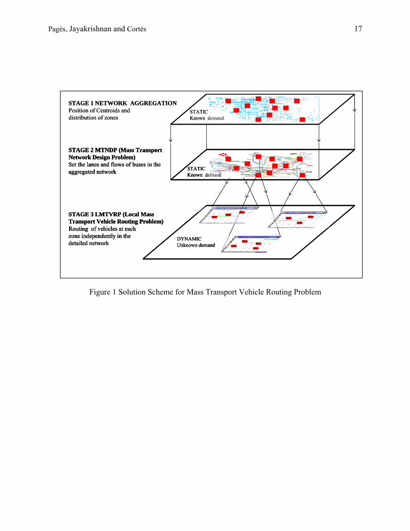
Solution Scheme for MTVRP Dynamic routing solutions have been found so far using approximations of static cases when the dimensions of the problem are small and/or using local heuristics when the dimensions get big. Generally, heuristics used for these types of problems do not consider global optimality. A procedure to solve the “MTVRP” through three different steps has been developed which seeks optimality by performing a hierarchical optimization. But the fact that the routing decisions are taken in real time does not allow the problem to have a closed form. Then, the optimization problem treated cannot be solved under a normal classical optimal control scheme because the formulation does not explicitly enumerate search directions at any of the solution points. Thus a question arises on how well the optimization schemes perform. Simulation of the optimization schemes seems to be the only viable way to study this complex problem. Due to the dimensions of the problem and the nonlinearities in the costs (passenger costs in vehicle rerouting depends on the load of vehicles), microsimulation is the plausible tool within this analysis. It is obvious that an implementation of a simulation platform for a demand-responsive transit system is needed. But it is not obvious how to simulate properly this transit system. Commercial packages are based primarily on modeling personal autos, and the capabilities needed to simulate flexible transit systems are not available in such software. Special purpose simulations have been considered in the past. (18) developed a macroscopic simulation framework for evaluating city logistics. The model is composed of two sub-models, a model for vehicle (pick-up/delivery truck) routing and scheduling problem with time windows and a dynamic traffic simulation model for the fleets of pickup/delivery trucks and passenger cars on the road network within the city. (19) simulates paratransit systems. Two types of trips are considered: advance reservation trips which are requested in advance and real-time trips which are requested after service starts and need to be serviced immediately. In this case, the simulation has no network associated. (20) described the implementation of different simulation modeling frameworks for new transit systems in PARAMICS. The scheme presented here is studied using this framework. The global optimization implemented in this research is now presented. It can be decomposed in three stages as shown in Figure 1 and further explained below. While the paper focuses on stage 2 of this optimization process, a brief description of each stage is necessary to understand the main aim of this research

< Insert Figure 1 here >


STAGE 1 - Network aggregation

In the first stage of this procedure the demand is grouped into zones in order to diminish the complexity of the network problem. Each zone in our studies has approximately 1.5 sq. miles of surface and has associated with it the following components: a) One Centroid (similar to Centroids in planning models) and b) groups of passengers with their associated origins-destinations trip desires. For brevity, this paper leaves out the details of this stage of the process. The networks considered are already aggregated.

STAGE 2 - MTNDP - Solution of the “Mass Transport Network Design Problem” (MTNDP)

Here “Mass Transport Network Design Problem” is solved. It is an acceptable static problem, which is a simplification of the proposed dynamic one in the aggregated network described above. The demand appearing in real time is not considered. The solutions of this stage are a set of “global” vehicle routes (or vehicle movement “corridors”) and their associated frequencies, which are used to develop an initial vehicle deployment pattern for stage 3. This paper focuses on this stage of the procedure and it is further explained below.

STAGE 3- LMTVRP Solution of the “Local Mass Transport Vehicle Routing Problem”

Each zone (corresponding to one centroid and, say, 10 vehicles) is taken independently. The number of vehicles being low, known vehicle routing heuristics are used to satisfy the demand appearing in real time. The cost function used is similar to the one used by Cortés (17), where the cumulative travel time of passengers in the system is taken into account. Unlike other public transportation design schemes, this modeling scheme does not consider passenger behavioral models at any stage (modal split is assumed given, and no other modes are considered in the optimization process). Under these circumstances, the solution is found by solving a flow minimization problem where the only path decision costs are based on passengers’ travel times. In other words, in a current solution, passengers are “forced” to use the vehicles of the proposed system and the path chosen will depend only on their travel and waiting times. Introducing a behavioral model into this scheme will be taken into consideration as part of further research, considering a real implementation of such a system. This paper now will focus on the important fundamental optimization problem in stage 2. First a description of the problem and its formulation are presented, followed by a solution for an example application.

Solution of the “Mass Transport Network Design Problem” (MTNDP) Formulation for MTNDP Consider a network represented by the directed graph G (N, A), with node set N and arc set A. The arcs here can be viewed as “global vehicle corridors” between nodes which represent “areas” (or even transfer hubs) in a large urban area. The intent is to find the “flow” (or frequency) of vehicle movement on these corridors, and to find how many vehicle travel on paths that go over such “nodes”, so that a global estimate can be made for mass transport vehicle movements. Note that the actual vehicle movements may involve local rerouting of these vehicles on actual network links for passenger and pick-up and delivery, as handled by the stage-3 of the scheme. The global path and flow solution and the associated vehicle deployment (mass transport network design) can then be used as the starting solution or the


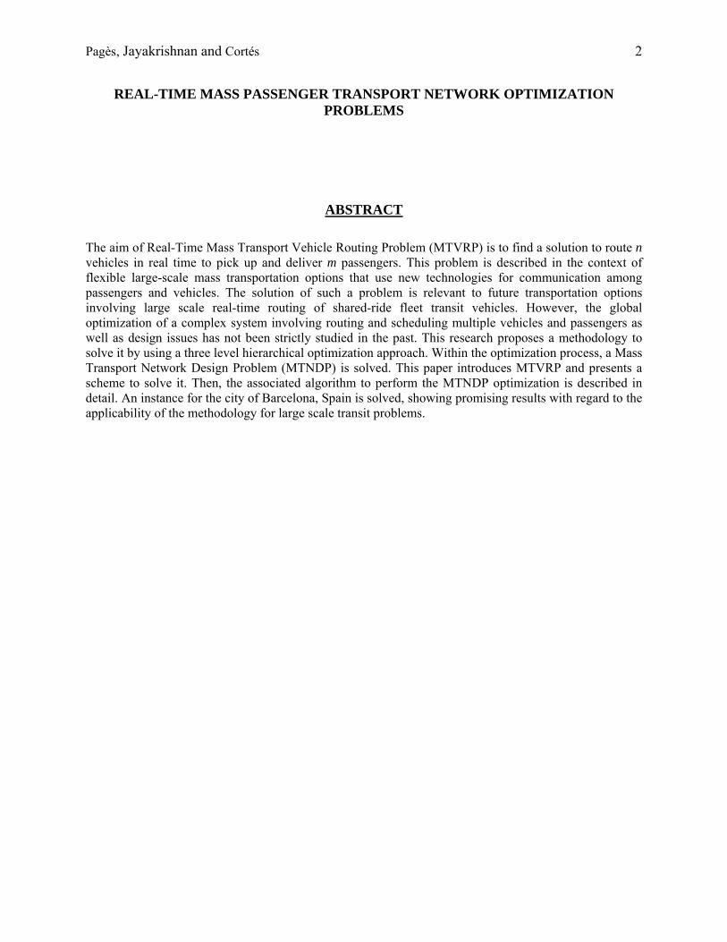
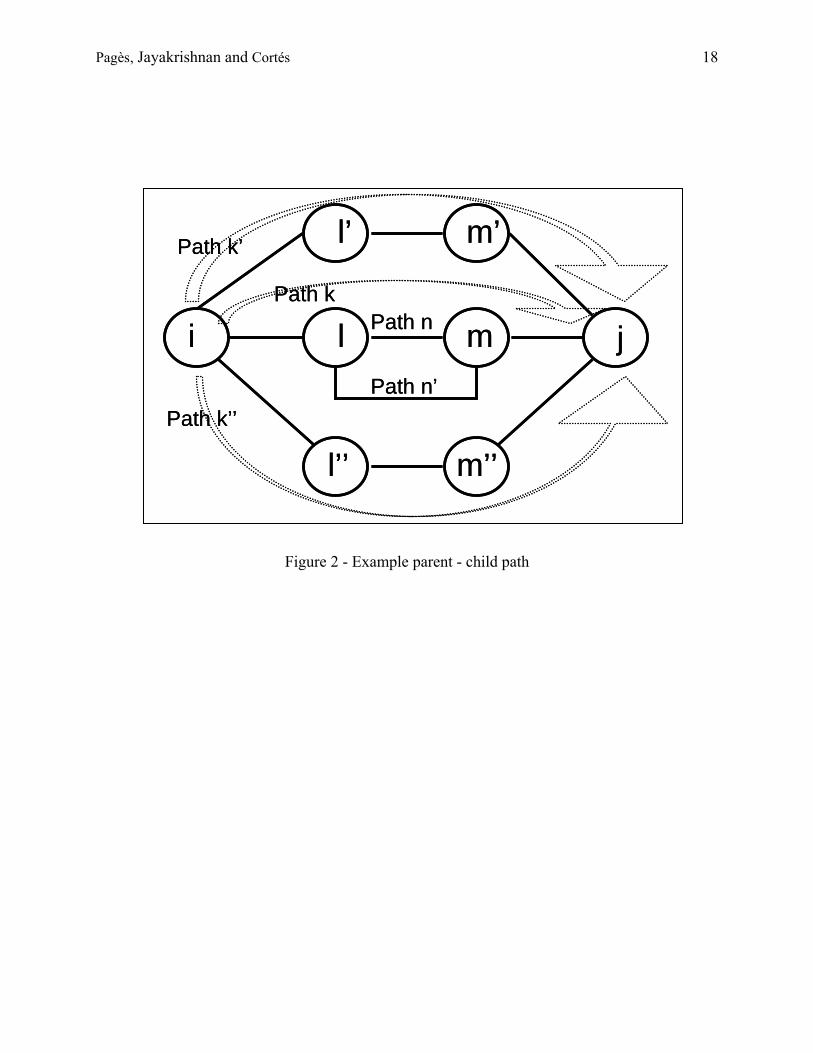
solution that set the global parameters for the LMTVRP problem (stage-3). One can also view MTNDP as solving the trunk route movement problem, if these vehicles are to have non-reroutable trunk route travel and re-routable local travel as in the HCPPT problem (17). The following discussion now focuses on these global “paths” and vehicle flows on them. Though we use the term “stops” as in the standard transit network design problem, these are not actual bus stops but are rather areas (represented by nodes) where vehicles enter the local streets or terminals rather than travel through as in express transit corridors. Thus the solutions would tell us how many vehicles travel from which areas in a large urban network to which other areas, at what type of frequency. The design thus provides us vehicle “routes” which can be viewed similar to bus lines or services in a bus network design problem, but are referring to global vehicle route corridors rather than bus lines or services with set schedules and frequencies. Consider a set of paths ( ijkp being the kith path starting at node i and finishing at node j). Some of the routes might have sub routes, which have both its origin and destination coinciding with intermediate vehicle stops of the longer vehicle routes. Let us call the long route “parent” and the sub route “child”. For the sake of clarity, Figure 2 draws a simplified example of paths ijkp , 'ijkp ''ijkp starting at node i and

ending at node j and paths lmnp and 'lmnp starting at node l and ending at node m. In this example, ijkp is a

parent of lmnp . <Insert Figure 2 here>

Mass Transport Network Design Problem (MTNDP) aims to find the routes and associated rates of vehicles to minimize the travel time of passengers (1). There are three sets of constraints. The first set of constraints (2) makes sure that all the demand is satisfied. The second group of constraints (3) are link capacity constraints valid for each line, assuring that the number of passengers traveling in one vehicle route (alternatively called a vehicle “line” or vehicle “service”) at a given time is smaller than the sum of all the available vehicle seats in that line. The last constraint (4) makes sure that the number of used vehicles is smaller than the fleet size. The formulation is the following:

lmnijk

lmnijk

lmnijklm

i j k l m n

lmijk wtttxfMinimize δ)( +∑∑∑∑∑∑

1=∑∑∑

i j k

lmijkf ml,∀ Continuity Constraint (1)

ijklmnijk

l m

almnlm

lmijk Crxf ≤∑∑ δφ kji ,,∀ Link Capacity Constraint (2)

Nrtt ijki j k

ijkijk ≤∑∑∑ Total Fleet Constraint (3)

ijkp = kth path between node i and node j

ijkr = rate of vehicles on path pijk (vehicles/unit time)

ijx = rate of demand from node i to node j (passengers/unit time)

lmnijktt = in-vehicle travel time from l to m using lmnp , child of ijkp (unit time)

lmnijkwt = waiting time from l to m using lmnp , child of ijkp (unit time)

lmijkf = fraction of demand lmx traveling on ijkp , parent of lmnp


lmnijkδ = 1 if lmnp is a child of ijkp , = 0 otherwise

aijkφ = 1 if ijkp goes over link a, = 0 otherwise

C = Vehicle capacity (passengers / vehicle) It is important to see that the objective function depends on the sum of waiting and travel time ( lmn

ijklmnijk wttt + ), while in constraint (4) only the travel time ( lmn

ijktt ) is considered. This is because the objective function represents time consumed by passengers, as opposed to the third constraint, in which only the travel time of vehicles is considered. Hence, waiting time does not need to appear in the third constraint because it does not have an effect on the vehicles travel time. Note however that it is precisely the presence of the waiting time in the objective function that makes MTNDP non-linear. the problem becomes linear only for a fixed set of routes and frequencies (in other words, for a given set of ijkr for all i, j and k) where the waiting times for each route are known. This characteristic has been exploited in the methodology explained in the next sections to solve MTNDP. An examination of the details would reveal some similarities between the MTNDP formulation and the well known Network Design Problem (NDP), studied by (21), (22), (23), (24), (25) and (26), among others. But there exist differences between MTNDP and NDP that make our problem easier to solve. MTNDP is not a subset or a simplified version of NDP; rather, these are just two different problems. The primary difference is that NDP is geared towards finding a network design that is immediately followed by frequency setting and scheduling, whereas the MTNDP finds a solution at an abstract (or aggregate) level composed of transit “flows”. Furthermore, the solution to MTNDP violates some of the basis for NDP, for example MTNDP identifies a situation without considering the return of the transit vehicles to the starting point of the vehicle route. The flow for each line “appears” at the origin of the line, and then travels along the route, picking up and dropping off passengers and later “disappears” at the destination (or terminus) of the line. Note that this would be impossible to implement in the real world, but its solution is what gives global optimality in the p[resent of local routing optimization. In terms of the theoretical details, NDP presents a concave (27) and multiobjective objective function arising from the fact that it tries to minimize both passenger and operator cost. Therefore, in the case of NDP, the tradeoffs among the conflicting objectives need to be addressed because it is multi-objective. But in MTNDP, only the passenger costs are minimized, therefore the objective function is simpler. Also, we do not accept transfers. Another difference is that the combinatorial explosion originating from the discrete nature of NDP is not present in MTNDP because its variables are continuous. Also, and perhaps most importantly, the network taken into account for MTNDP is an aggregated one; therefore the sizes of the networks needed are relatively small compared to the networks solved by researchers working on NDP (28). Finally, our problem aims to create a transit system from scratch, whereas, in general, the most conventional NDP schemes starts from an already created system adding new lines and/or changing the existing ones to optimize the system.. To further explain, imagine a “rate of passengers” willing to travel from the origins to the destinations. The solution for MTNDP is the vehicle “lines” and the associated frequencies to perform these operations with a minimum user cost. Therefore, our interest is to find the “lines” (which can be viewed as loose collection of fleet vehicles operating in some corridors) and vehicle frequencies between each OD pair, minimizing the travel time of users with two restrictions: a given fleet size (a), a maximum vehicle capacity (b). The length of the routes and the frequencies of the vehicles identify the vehicle deployment and trunk/express travel patterns in different areas of a real world network. In the next section, the steps performed to find a solution are described and an example is presented.


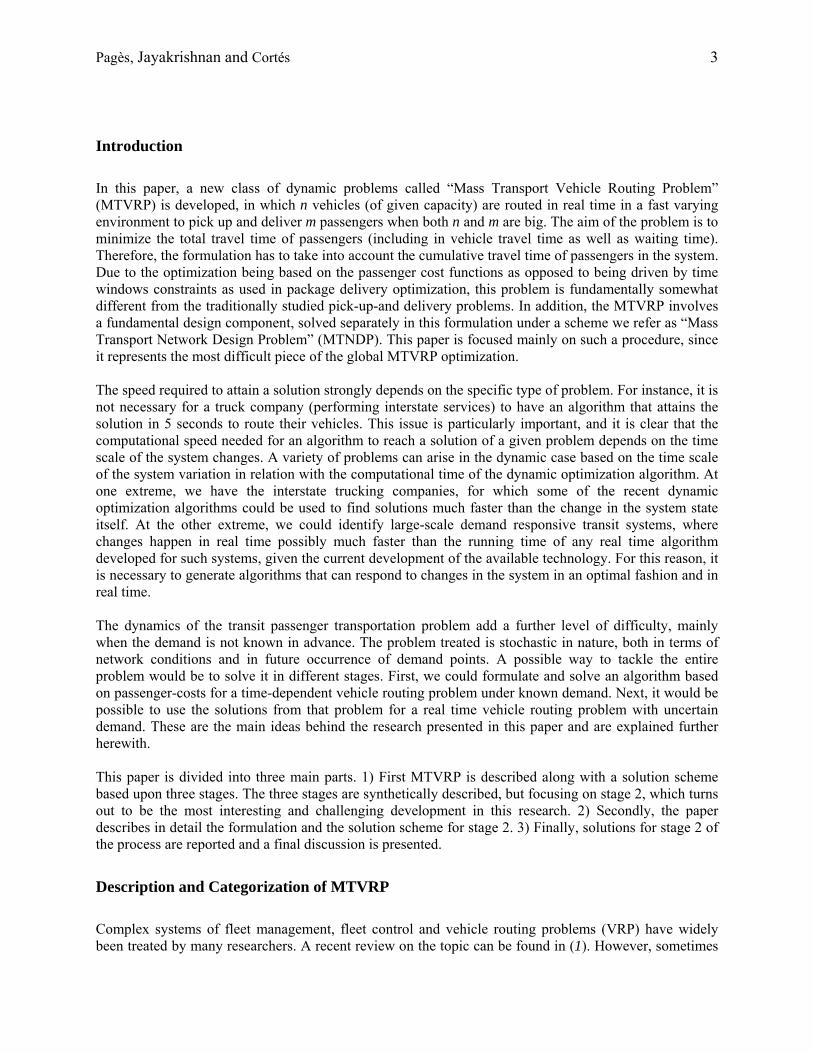
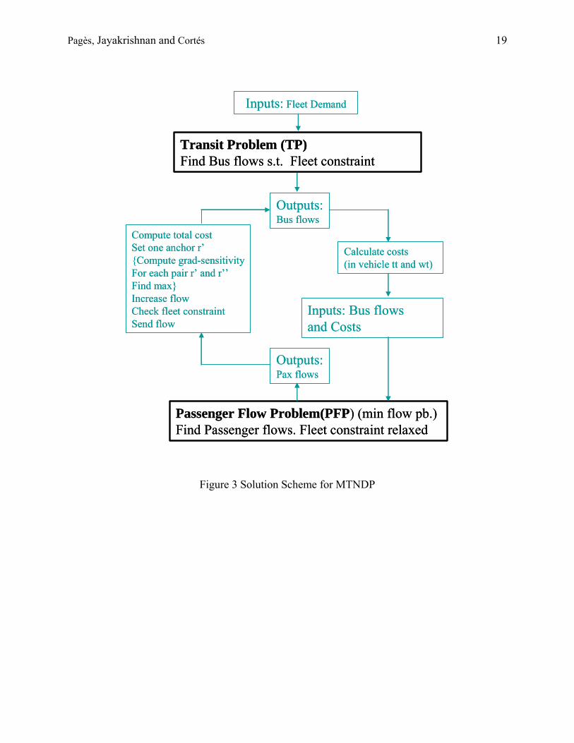
Solution Scheme for MTNDP MTNDP is a minimum cost flow problem consisting of two levels. In the first level (we call it “Transit Problem” or TP), there are vehicle flows, or “empty seats” flows. In the second level (we call it “Passenger Flow Problem” or PP) there are passenger flows. Seat flows are not explicitly present in the objective function, but passenger flows depend on vehicle flows because it is obvious that vehicle flows cannot be smaller than passenger flows at any point. In order to deal with this scenario, an iterative process is proposed where first a set of vehicle flows are found in a relaxed form of TP and then, for this fixed set of vehicle flows, the best set of passenger flows is found in the PP. Once the TP and PP are solved, we have a feasible solution, (in other words we have a set of both vehicle and passenger flows). At this point, we start the procedure again: we try to find a better set of vehicle flows (solution of TP) that improve the overall solution and fix them. For this fixed set of vehicle rates, the best passenger flows are calculated. These operations are performed successively until no more improvements are found. Figure 3 shows the implemented procedure used to solve MTNDP. In the rest of this chapter, the parts of the problem shown Figure 3 are explained in detail.

<Insert Figure 3 here>

The MTNDP is a non-linear function. As noted above, non-linearity in the objective function is induced by travel time ( lmn

ijklmnijk wttt + ), which includes the in-vehicle travel time ( lmn

ijktt ) and the waiting time

( lmnijkwt ). Furthermore, the expected waiting time for a given passenger is inversely proportional to the rate

of vehicles in the line (corridor) where he or she is traveling. For the purposes here, we conservatively assume that lmn

ijktw = 1/ ijkr , though this depends on the vehicle headway distribution, as is well-known (and furthermore, this waiting time depends on the local real-time routing heuristics in any event). It is clear however that the non-linearity of this function arises from the waiting time. Now, once the set of routes and the frequencies are known, (i.e., a feasible solution for the TP), then the vehicle rates are fixed, the waiting times are not variables anymore: they become just known constants, thus the objective function has a linear form. That is, for fixed (temporary) costs and vehicle rates, our problem is linear. Now the TP and PP are treated separately in the next sections and then the iterative process between TP and PP is described. Transit Problem (TP) TP finds a set of routes and associated frequencies to satisfy a given demand pattern. It is solved using a heuristic described above. It is important to note at this point that the heuristic is solved only once and its solution used as an initial solution for the iterative process; as it can be seen in Figure 3 shown above.

STEP 1- Feasible initial solution: A frequency is associated with each transit vehicle line with positive demand. Vehicle rates are set to its “minimum desired rate” from each node i to each other node j which is equal to the rate of demand of passengers traveling from i to j, multiplied by cost from i to j and divided by the passenger capacity of vehicle units (the number of seats).

The solution obtained under the “minimum fleet needed” step is feasible because all the constraints are satisfied, but it is sub optimal because each passenger (nodal O-D pair) is using a line with the termini at the two nodes. On the other hand, under this solution, all vehicles are full all the time. Hence, the number of vehicles needed in this solution (let us call it F1) is expected to be lower than the optimal solution.


STEP 2- Transit vehicle route integration: For each arc of each parent route, the rate of vehicles for the parent route is set equal to the maximum of the sums of all the rates needed for all child routes. The operation is performed for all parent routes with a maximum preset number of links, starting by the parent route with the highest number of child routes. The procedure checks the fleet constraint at each increase of vehicle flows. This step of the process eliminates redundant lines and creates empty space in parent line’s vehicles. Let us call the fleet size needed in this step of the process F2. In any case F1 < F2, but neither is larger than the maximum fleet size (N) fixed in the MTNDP formulation.

STEP 3- Transit vehicle route truncation: Once rates for all parent routes are set, child routes are not needed anymore. But, if all child routes were cancelled, the resulting network would only be composed of high frequency parent routes and the fleet constraint might be violated. Equilibrium between parent routes and child routes is achieved here by canceling the child routes which have a lower rate than a predefined value and setting the rest of the child rates to a variable fraction of its previous rate. Let us call the fleet size used in this situation F3. Note that F3 > F1 and F3 < F2. Again, none of the fleet sizes are larger than the maximum fleet size N.

Once the above heuristic is completed, the PP problem can be optimized. The original network topology is changed to take into account the operational restrictions of the vehicles introduced in our model. First of all, transfers are not allowed. Secondly, we are routing vehicles as if they were taking part of a public transportation service line, therefore passengers who are traveling in a sub-path of any longer path can enter into a vehicle that is serving the bigger path but not vice versa. An “expanded” network depicting these phenomena is built, for use in the linear multicommodity flow optimization in the PP problem that follows. Each OD is represented by a super sink and a super source, corresponding to one commodity and each considered path is represented separately. The TP solution allows the computation of the expected passenger waiting time for each line. A matrix with all the waiting times for each line is computed and is fed into PP, explained in the next section. Passenger Problem (PP) For a given set of vehicle rates, the waiting times for all routes are known and PP becomes a Linear Multicommodity Minimum Cost Flow Problem, (LMMCFP) dealing only with a unique set of variables: passenger flows. The well-known network simplex schemes can be implemented on the expanded network. Each origin-destination pair is treated as a different commodity. LMMCFP have been solved in the past either with partitioning methods, resource directive or price directive decomposition methods. Lately other algorithms have been developed such as the interior point methods (29). According to (30), (31) and (32), price directive decomposition methods perform better when a lot of commodities are considered; therefore a variant of this method has been implemented in this research. Price directive decomposition eliminates the bundle constraints in the matrix by placing prices to these constraints and introducing them into the objective function. The resulting system is a relaxed “minimum flow cost problem” for each commodity. The problem has a dual variable for each arc ( aw ) corresponding to the continuity constraint and a dual variable for each commodity ( kσ ) corresponding to the link capacity constraint. Following this formulation, a pricing problem is solved at each step. If the complementary slackness conditions hold, then the solution is optimal and the procedure stops, otherwise,


a new pricing problem is solved until an optimal solution is found. Interested readers are directed to (33) and (34). Iterative Process In the previous sections, both TP and PP have been described and their solution schemes have been presented separately. Both solutions are useful for our ultimate goal, but need to be combined in order to obtain a solution for the MTNDP. The last part of the scheme, which ties both problems and finds the solution for MTNDP, is introduced in this section. A particular implementation of a steepest descent method has been coded to optimize the problem. The essential idea behind our gradient-search is that each solution of TP gives one point in the solution space and the objective value for the MTNDP problem presented in equations (1) to (4). The optimization finds the gradient using a perturbation of the solution and the global optimization proceeds using a steepest descent method. The reason why this procedure is selected is that the TP solution can be found relatively easily using the LLMCFP scheme. This explains the need for us to split the optimization problems to two subproblems, PP and TP. The procedure is as follows: Start with a solution of the TP and PP and call the cost of the overall problem

,...),...,,...,,,...,,( '''''''''212211122121 kjikji rrrrrrF . An “anchor” path ''' kjip is chosen and its rate ''' kjir fixed to

''' kjir +∆r. Now, each one of the remaining paths '''''' kjip (different than ''' kjip ) is considered independently

and a unit of vehicle flow is decreased in '''''' kjip , setting the new rate to. '''''' kjir -∆r. For this new situation,

the value for F( ,....,, 122121 rr ,....,, 212211 rr ''' kjir +∆r,…, '''''' kjir -∆r, …) is computed. Then the gradient for

each pair “ ''' kjip - '''''' kjip ” can be written as follows:

r

rrrFrrrrrFr

F jkikjijkikji

kji ∆−∆−∆+

=∂∂ ,...),..., ,...r,...,r,(,...),..., ,...r,...,r,( '','','''''211122121'','','''''211122121

''''''

Once this operation has been performed for each '''''' kjip , it is possible to write the gradient vector as follows:

⎟⎟⎠

⎞⎜⎜⎝

⎛

∂∂

∂∂

∂∂

∂∂

∂∂

∂∂

=∂∂ ,...,....,,...,,,

212211123122121 ijkrF

rF

rF

rF

rF

rF

rF

.

At this step, a new cost is computed where the new objective function is then:

NewrFrrrrrrFF kjikji ∂∂

−= λ,...),...,,...,,,...,,( '''''''''212211122121

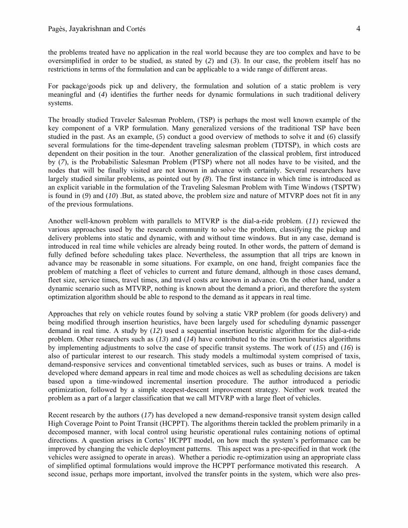
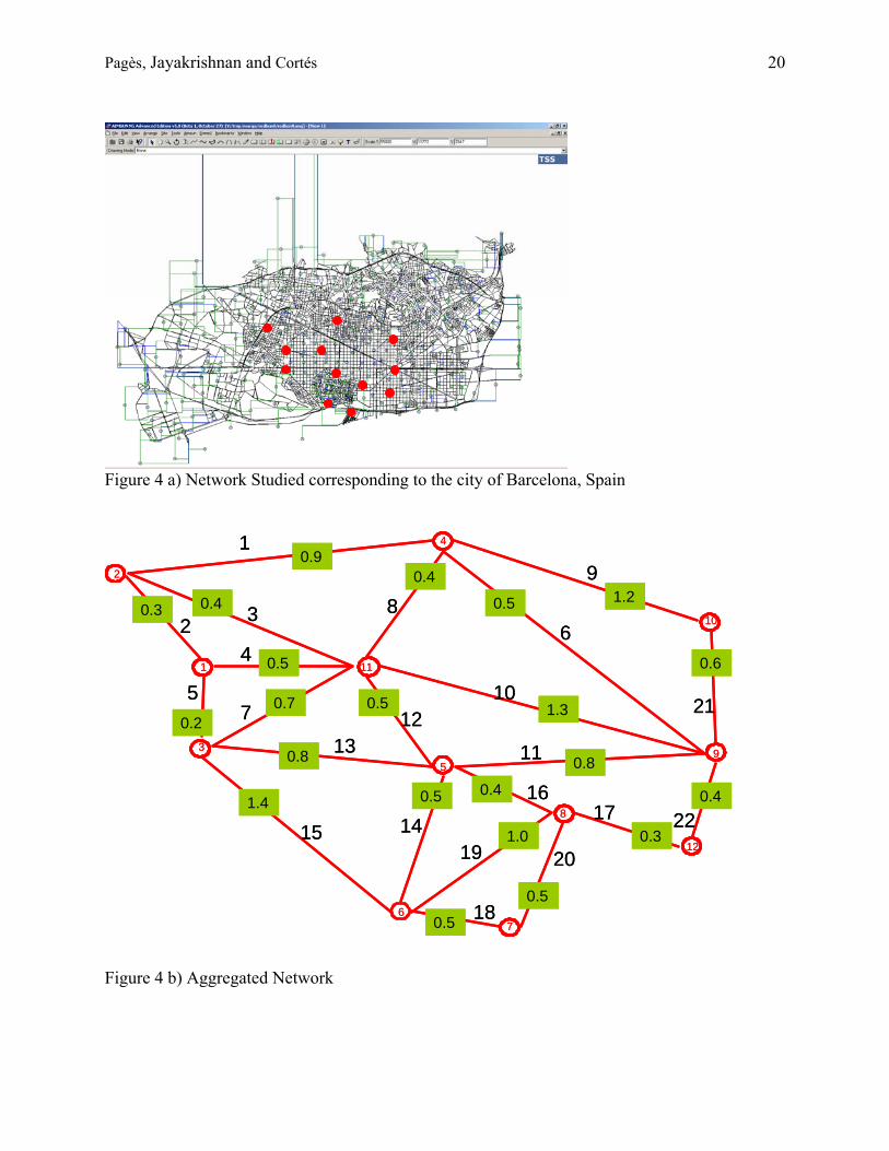
The algorithm runs until optimality is attained. Next section shows the results for one of the cases treated. Numerical Application A network corresponding to the city of Barcelona in Spain has been chosen as an example to solve MTNDP through the methodology explained in the previous sections. Figure 4 shows the original network and the remaining network after performing the aggregation of the nodes into centroids. The node numbers, link numbers and the corresponding in-vehicle travel costs (in green) are also shown in the


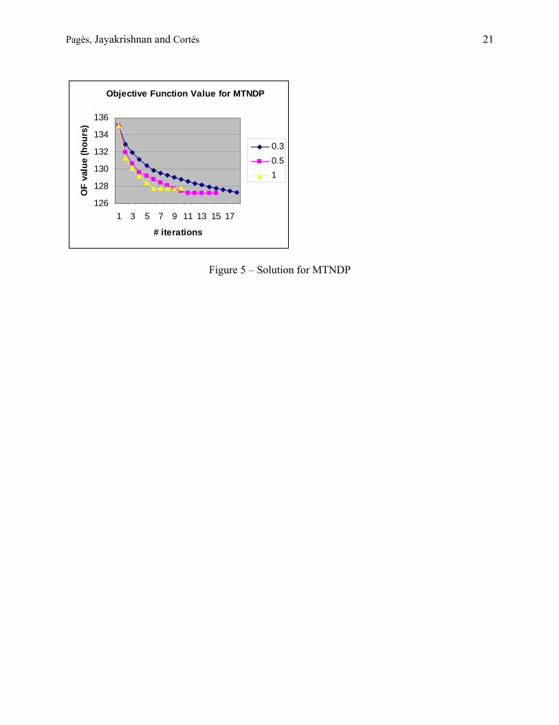
same figure. Note that the nodes of the aggregated network correspond to the main hubs of the existing underground network. Also, the links correspond to “global vehicle corridors” which do not have to coincide exactly with the existing roads of the city, because the aim of the aggregated network is just to simplify the real network and diminish the number of nodes and links. In all the scenarios considered, vehicle capacity was set to 5 passengers and the integration was done for paths with more than 2 nodes (in other words, path integration was performed for all the paths considered in this network). The code was run for different values of λ and different numbers of iterations. The values of the Objective function for MTNDP for these different settings are presented in Figure 5.

< Insert Figure 5 here> The Figure shows a decreasing trend for all curves, meaning that the sum of travel times for all passengers in the system improves in all the studied cases, starting at the same initial solution and finishing at similar solutions. Note that the values of the Objective functions for the first iteration are the same for all scenario runs. This is normal since the first iteration only depends on the solution of the TP, which, for all cases is the output of the heuristic explained above. Figure 5 shows that for all curves, there is a threshold value, after which the solution does not improve anymore, even if we continue to iterate. At this point, optimality has been achieved and the algorithm stops. Notice that, the final solution is not exactly the same in all situations. A first observation would be that the smaller the ∆r, the smother the convergence rate is and the more accurate the final solution is. This result is consistent with the intuitive thought that if “small” changes are performed in vehicle rates, the changes in passenger flows are also small, giving a more accurate solution, while if only “big” changes on rates are performed, then only a subset of passengers can travel through their best path, resulting in a suboptimal objective function value. Also, it is easy to realize that for small ∆r, the curves are smoother than for big ∆r. Again, is intuitive to think that when ∆r is small, each step of the algorithm is going to improve the solution by a small amount, drawing a smooth curve. On the other hand, when ∆r is big, each step of the algorithm is going to give a bigger change on passenger paths and passenger travel times, resulting in a less smooth curve as shown in the figure. The slope of the curves is much higher at the beginning of the algorithm than at the end, meaning that for a given experiment, the improvement of the solution for the first iterations is much higher than for the lasts iterations. In the first iteration after the initial solution, waiting times are introduced in the system for the first time, making the travel times of passengers higher and, in some cases, completely different. Therefore, it is normal that in the first iterations, the changes in vehicle rates implies a big change in passenger costs. After the initial iterations, the influence of waiting times is “stabilized” and the changes over the vehicle rates do not have such a big influence on passenger’s costs. Then, the improvements on the objective function for each step of the algorithm becomes smaller. As expected, the time required for more accurate solutions is much higher than that for the the less accurate solutions. The computational time taken by our code was compared with the time taken by CPLEX. For data on computational times and a discussion on these issues refer to (35).


Conclusions and further research The main contribution of this paper is identifying a new problem called “Real Time Mass Transport Vehicle Routing Problem” and describing a solution algorithm. The solution scheme for MTVRP involves solving an associate problem called “Mass Transport Network Design Problem” (MTNDP). This paper also describes MTNDP problem, shows its formulation and presents results on the application of the algorithm. This methodology is expected to be of use for the academic community to solve large scale dynamic routing problems. Forthcoming research is expected in MTVRP introducing improvements in stage 3, which was not developed in detail in this paper. As far as MTNDP is concerned, the solution scheme for it has been implemented using a steepest descent algorithm which seeks optimality by performing small changes in the vehicle flows and looking into the costs of passenger flows. But, this is only one of the possible solution methods for MTNDP. Inspired by the particular form of the problem, in the future it would be worth trying to solve MTNDP by using a Benders decomposition approach by dividing the linear part and the non-linear part of the objective function of the problem. Acknowledgements This research was partially financed by CALTRANS, the Henry Samueli School of Engineering at the University of California, Irvine, the University of California Transportation Center (UCTC), the California Catalonia Program. Balsells - Generalitat de Catalunya Fellowhip. Catalunya. Spain, Fondecyt, Chile, grant 1030700 and the Millennium Nucleus "Complex Engineering Systems". The authors would like to thank Jaume Barceló (Department of Statistics and Operations Research, Universitat Politècnica de Catalunya, Spain) for his valuable comments.

References

1. Bräysy O. and Gendreau M. Vehicle Routing Problem with Time Windows, Part I: Route Construction and Local Search Algorithms. Transportation Science. Vol. 39 No. 1, 2005, pp 104-118 2. Bodin, L.D. Twenty years of routing and scheduling. Operations Research, Vol. 38, 1990.pp. 571-579, 3. Hang Xu, Zhi-Long Chen, Srinivas Rajagopal, Sundar Arunapuram. Solving a Practical Pick up and Delivery Problem. Transportation Science, Vol 37, No. 3, 2003, pp. 347-364. 4. Psaraftis H. Dynamic Vehicle Routing Problems. Vehicle Routing: Methods and Studies. B. L. Golden and A.A. Assad (Editors). Elsever Science Publishers B.V. 1988. 5. Laporte, G. The Traveling Salesman Problem: An overview of Exact and Approximate Algorithms. European Journal of Operational Research Vol. 59, 1992, pp. 231-247. 6. Gouveia L., Voβ S. A classification of formulations for the (time-dependent) traveling salesman problem. European Journal of Operational Research Vol. 83, 1995, pp. 69-82. 7. Jaillet, P. A Priori Solution of a Traveling Salesman Problem in which a random subset of the customers are visited. Operations Research Vol. 18, 1988, pp. 51-70.


8. Laporte et al. New insertion and Postoptimization procedures for the Traveling Salesman Problem. Operations Research Vol. 40, 1992, No. 6. 9. Gendreau M. Hertz A. Laporte G. and Stan M. A Generalized Insertion Heuristic for the Traveling Salesman Problem with time windows. Operations Research Vol. 43, No. 3. May – June 1998.

10. Salomon et al. Solving the discrete lot sizing and scheduling problem with sequence dependent set-up costs and set-up times using the Traveler Salesman Problem with Time Windows. European Journal of Operational Research Vol. 100, 1997, pp. 494-513. 11. Savelsberg, M.W.P. and Sol. The general pickup and delivery problem. Transportation Science Vol. 29(1), 1995, pp.17-29. 12. Jaw et al. A heuristic algorithm for the multi-vehicle advance request dial-a-ride problem with time windows. Transportation Research Part B Vol. 20B No. 3, 1986, pp 243-257. 13. Quadrifoglio L., Dessouky M., Palmer K. An Insertion Heuristic for Scheduling MAST Services, Presented at UCTC conference, Irvine, February 2005. Submitted for publication in Journal of Scheduling.

14. Diana and M. Dessouky. A new Regret Insertion Heuristic for Solving Large-Scale Dial-a-Ride Problems with time windows. Transportation Research Part B Vol. 38, No. 6, 2004 pp. 539-557

15. Horn, M.E.T. Multi-modal and demand-responsive passenger transport systems: a modeling framework with embedded control systems. Transportation Research Part A Vol. 36, 2001, pp.167-188.

16. Horn, M.E.T. Fleet scheduling and Dispatching for Demand Responsive Passenger Services. Transportation Research Part C, Vol 10, No. 1, 2002 pp. 35-63.

17. Cortes C. Ph D. Dissertation. High-Coverage Point-to-Point Transit (HCPPT): A new design concept and simulation-evaluation of operational schemes for future technological deployment” UCI, 2003. 18. Taniguchi et al. City Logistics. Pergamon Elsevier Science Tokyo. 2001. 19. Fu L. Scheduling dial-a-ride paratransit under time-varying, stochastic congestion. Transportation Research Part B 36 pp. 485-506. 2002.

20. Cristián Cortés, L. Pagès and R. Jayakrishnan, Microsimulation of Flexible Transit System Designs in Realistic Urban Networks Presented at the 84nd Annual Meeting of the Transportation Research Board Meeting, Washington D.C. 2005 and forthcoming Publication in Transportation Research Record.

21. Mandl C. Evaluation and optimization of urban public transportation networks. European Jorurnal of Operational Research Vol 5, 1980, pp. 396-404. 22. Hasselstrom. Public Transportation Planning – A mathematical programming approach. PhD Dissertation. Department of Business Administration, University of Gothemburg, Sweden 1981.


23. Ceder and Wilson Bus Network Design. Transportation Research, Vol. 20B, 1986, pp 331-344. 24. Baaj and Mahmassani Hybrid Route Generation Heuristic Algorithm for the design of Transit Networks. Transportation Research Vol 3, No. 1, 1994, pp 31-50. 25. Cynthia Bahnhart, Hong Jin and Pamela H. Vance. Railroad Bocking: A network Design Application. Operations Research Vol. 48, No. 4, 1998, pp 603-614. 26. Rob Van Nes. Multi user-class urban Transit Network Design. Presented at the 82nd Annual Meeting of the Transportation Research Board Meeting, Washington D.C. January 12-16, 2003

27. Newell, G. Some issues related to the optimal design of bus routes. Transportation Science, Vol.13, 1979, pp. 20-35.

28. Cynthia Barnhart, et al. Composite Variable Formulations for Express Shipment Service Network Design. Transportation Science Vol.36, No.1, 2002, pp.1–20

29. Karmarkar N K (1984) A new polynomial time algorithm for linear programming. Combinatorica 4: 373–395

30. Kennington J L (1978) A Survey of Linear Cost Multicommodtiy Network Flows. Operations Research 26(2): 209–236

31. Ali A, Helgason R V, Kennington J L , Lall H , (1980) Computational comparison among three multicommodity network flow algorithms. Operations Research 28: 995–1000

32. Ahuja, R K, Magnanti, T L, Orlin, JB (1993) Network Flows. Prentice Hall, Englewood Cliffs, New Jersey

33. Kennington J L, Helgason RV (1980) Algorithms for network programming. John Wiley & Sons, New York

34. Kim, Barnhart C (1999) Multimodal Express Package Delivery: A service Network Design Application. Transportation Science Vol 33, No. 4: 391-407

35. Pagès and Jayakrishnan. Mass Transport Vehicle Routing Problem (MTVRP) and the Associated Network Design Problem (MTNDP). Accepted for presentation at the International Scientific Annual Conference Operational Research Bremen. Germany. 9-13 September 2005


LIST OF FIGURES

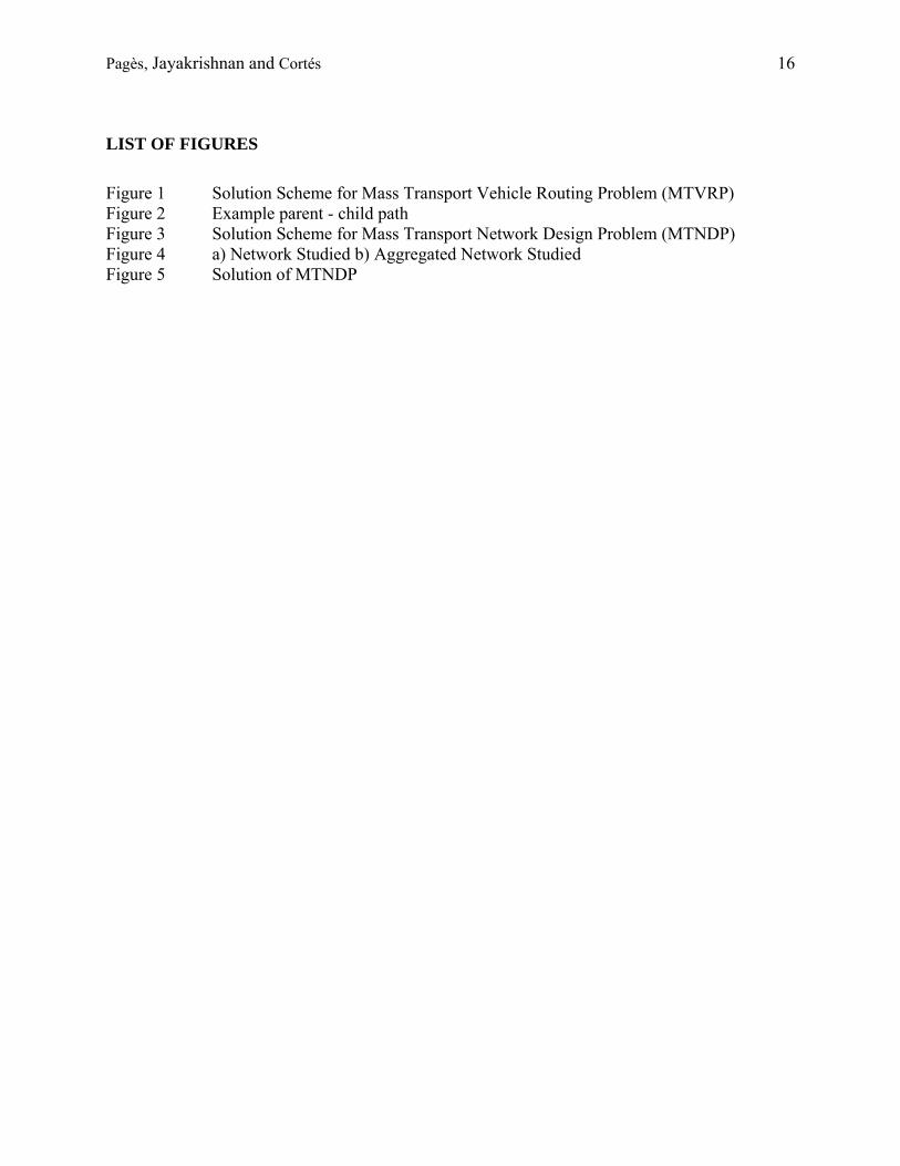
Figure 1 Solution Scheme for Mass Transport Vehicle Routing Problem (MTVRP) Figure 2 Example parent - child path Figure 3 Solution Scheme for Mass Transport Network Design Problem (MTNDP) Figure 4 a) Network Studied b) Aggregated Network Studied Figure 5 Solution of MTNDP


Figure 1 Solution Scheme for Mass Transport Vehicle Routing Problem

STAGE 1 NETWORK AGGREGATIONPosition of Centroids and distribution of zones

STATICKnown demand

STAGE 2 MTNDP (Mass Transport Network Design Problem)Set the lanes and flows of buses in the aggregated network STATIC

Known demand

STAGE 3 LMTVRP (Local Mass Transport Vehicle Routing Problem)Routing of vehicles at each zone independently in the detailed network

DYNAMICUnknown demand

STAGE 1 NETWORK AGGREGATIONPosition of Centroids and distribution of zones

STATICKnown demand


Known demand


Known demand






Figure 2 - Example parent - child path

i jl m

l’ m’

l’’ m’’

Path kPath n

Path n’

Path k’

Path k’’

i jl m

l’ m’

l’’ m’’

Path kPath n

Path n’

Path k’

Path k’’


Transit Problem (TP)Find Bus flows s.t. Fleet constraint

Inputs: Fleet Demand

Outputs:Bus flows

Passenger Flow Problem(PFP) (min flow pb.) Find Passenger flows. Fleet constraint relaxed

Inputs: Bus flows and Costs

Calculate costs (in vehicle tt and wt)

Outputs:Pax flows

Compute total costSet one anchor r’{Compute grad-sensitivityFor each pair r’ and r’’Find max}Increase flowCheck fleet constraintSend flow

Transit Problem (TP)Find Bus flows s.t. Fleet constraint

Inputs: Fleet Demand

Outputs:Bus flows

Passenger Flow Problem(PFP) (min flow pb.) Find Passenger flows. Fleet constraint relaxed

Inputs: Bus flows and Costs

Calculate costs (in vehicle tt and wt)

Outputs:Pax flows

Compute total costSet one anchor r’{Compute grad-sensitivityFor each pair r’ and r’’Find max}Increase flowCheck fleet constraintSend flow

Figure 3 Solution Scheme for MTNDP


Figure 4 a) Network Studied corresponding to the city of Barcelona, Spain Figure 4 b) Aggregated Network

1

2

3

4

5

67

8

9

10

11

12

11

2

1

5

4

3

10

9

8

7

6

1213

1415

1617

18

19

21

20

0.9

0.2

0.3

0.5

0.5 1.20.4

1.0

1.4 0.5

0.8

0.6

0.8

1.3

0.4

0.5

0.5

22

0.7

0.4

0.5

0.4

0.3

1

2

3

4

5

67

8

9

10

11

12

11

2

1

5

4

3

10

9

8

7

6

1213

1415

1617

18

19

21

20

0.9

0.2

0.3

0.5

0.5 1.20.4

1.0

1.4 0.5

0.8

0.6

0.8

1.3

0.4

0.5

0.5

22

0.7

0.4

0.5

0.4

0.3


Objective Function Value for MTNDP

126

128

130

132

134

136

1 3 5 7 9 11 13 15 17

# iterations

OF

valu

e (h

ours

)

0.30.51

Figure 5 – Solution for MTNDP

Real-Time Mass Passenger Transport Network Optimization Problems

Documents