Real-time lookahead control policies

Real-time Lookahead Control Policies

Vadim Bulitko and Ilya Levner and Russ GreinerDepartment of Computing Science

University of AlbertaEdmonton, Alberta T6G 2H1

CANADA{bulitko|ilya|greiner}@cs.ualberta.ca

Abstract

Decision-making in practical domains is usuallycomplex, asa coordinated sequence of actions is needed to reach a sat-isfactory state, andresponsive, as no fixed sequence worksfor all cases – instead we need to select actions after sensingthe environment. At each step, alookahead control policychooses among feasible actions by envisioning their effectsinto the future and selecting the action leading to the mostpromising state.

There are several challenges to producing the appropriatepolicy. First, when each individual state description is large,the policy may instead use a low-dimensionalabstractionofthe states. Second, in some situations the quality of the finalstate is not given, but can only be learned from data.

Deeper lookahead typically selects actions that lead tohigher-quality outcomes. Of course, as deep forecasts arecomputationally expensive, it is problematic when compu-tational time is a factor. This paper makes this accu-racy/efficiency tradeoff explicit, defining a system’s effective-ness in terms of both the quality of the returned response, andthe computational cost. We then investigate how deeply asystem should search, to optimize this “type II” performancecriterion.

Keywords: Decision-making, control policy, lookahead statetree expansion, abstraction, responsive image recognition,real-time best-first heuristic search, search horizon.

1 Real-time Decision-MakingWe will start with a motivating practical example. Hav-ing detailed inventories of forest resources is of tremen-dous importance to forest industries, governments, and re-searchers. It would aid planning wood logging (plantingand cutting), surveying against illegal activities, and eco-system and wild-life research. Given the dynamic natureof forest evolution, the task of forest mapping is a continu-ous undertaking, with the objective of re-mapping the esti-mated 344 million hectares of Canadian forests on a 10-20year cycle. Remote-sensing based approaches appear to bethe only feasible solution to inventorizing the estimated1011

trees. Despite numerous previous attempts (Gougeon 1993;Larsen et al. 1997; Pollock 1994), no robust forest mappingsystem exists to date.

We have been developing such a forest inventory map-ping system (FIMS) using a set of sophisticated computer

Copyright c© 2002, American Association for Artificial Intelli-gence (www.aaai.org). All rights reserved.

vision operators. FIMS problem-solving state is representedusing a layered shared data structure as shown in Figure 1.Initially, aerial images and LIDAR data are deposited at thesensory input layer. As the computer vision operators areapplied, higher layers become populated with extracted data.Finally, the top layer gains the derived 3D interpretation ofthe forest scene. At this point the scene can be renderedback onto the sensory layer to be compared with the originalimagery to assess the quality of the interpretation.

In nearly every problem-solving state several computervision operators can be applied. Furthermore, each of themcan be often executed on a subregion of interest in its in-put datum. Escalating the choice problem complexity evenhigher, the operators sometimes map a single input to severalalternative outputs to select from.

In order to address the numerous choice problems a con-trol policy guiding operator application is necessary. Asdemonstrated in (Draper et al. 2000), a dynamic control pol-icy can outperform manually engineered fixed policies bytaking into account feedback from the environment. In eachcycle the control policy chooses among applicable operatorsby selectivelyenvisioning their effects several plies ahead. Itthen evaluates the states forecasted using itsheuristic valuefunctionand selects the operator leading to the most promis-ing state.

Deeper lookahead can often increase the quality of theapproximate value function used to compare predictedproblem-solving states (Korf 1990). Unfortunately, the typeII performance (Good 1971) that explicitly takes computa-tional costs into account is negatively affected as the num-ber of envisioned states grows rapidly with the lookaheaddepth. As we will show in section 6, an adaptive lookaheaddepth selection might be necessary to optimize the overalltype II performance and make the system runnable inreal-time(e.g., on-board a surveillance aircraft).

In FIMS operators are applied to traverse the problem-solving state space. Furthermore, immediate rewards canbe assigned to operator applications. Therefore, FIMS canbe thought of as an extension of the classical Markov Deci-sion Process (MDP) (Sutton et al. 2000) framework alongthe following directions: (i) feature functions for state spacereduction, (ii) machine learning for the value function anddomain model, and (iii) explicit accuracy/efficiency tradeofffor performance evaluation.

This paper presents work in progress with the follow-ing research objectives: (i) creating a theory and a practi-

1

Sensory Input

Extracted Features

Probabilistic Maps

Canopy Clusters

3D Scene Interpretation

Feature Feature Extractor 1Extractor 1

Feature Feature Extractor nExtractor n

…

Labeler 1Labeler 1 Labeler nLabeler n…

Grouper 1Grouper 1 Grouper nGrouper n…

ReconsRecons--tructor 1tructor 1

… ReconsRecons--tructor ntructor n

Projector Projector

Figure 1:Forest Inventory Mapping System (FIMS) is based on a layered data representation. Raw sensory data such as aerialimages are deposited at the bottom layer. As various computer vision operators are applied higher layers become populatedwith derived data. The output of the system is formed at the top layer and is then projected back into 2D for quality assurance. Inaddition to deciding among operators (e.g., feature extractor #5 vs. feature extractor #12) their inputs often need to be decidedon as well (e.g., image subregion #1 vs. image subregion #87).

cal implementation of an adaptive lookahead depth selec-tion module, (ii) studying machine learning methods forvalue function and domain model approximation within thelarge-scale FIMS application, (iii) comparing the adaptiveenvisionment-based control policy for FIMS with traditionalhand-crafted scene interpretation strategies.

The rest of the paper is organized as follows. Section 2describes the challenges we faced in producing this system– many due to our efforts to make the real-world system,with its mega-byte state information, run efficiently. Wethen (section 3) present a best-first lookahead control pol-icy guided by an approximate MDP value function. Thesection discusses its advantages over optimal goal-seekingalgorithms such as A* as well as the challenges in the formof value function inaccuracies. Section 4 discusses type IIoptimality which explicitly combines performance qualityand computational time and poses the specific problem wewill address in this paper: automatically determining the ap-propriate depth of the search. Section 5 then provides anempirical study to help us address this problem. Here wefirst present the artificial ”grid world” domain, and explainwhy this domain is rich enough to capture the challenges ofthe FIMS system, while remaining sufficiently constrainedthat we can obtain precise numbers. We then draw severalimportant conclusions in section 6 and consider related re-search in section 7.

2 ChallengesLike many real-world systems, the FIMS control policy isfaced with several formidable challenges including:

Ill-defined goal states. In FIMS, a goal system state con-tains an accurate interpretation of the forest scene ob-served. Unfortunately, such a state is impossible to recog-nize since the sought forest maps are typically unknown.The lack of recognizable goal states means that we cannotuse optimal goal-searching algorithms such as A*, IDA*,RBFS, etc. (Korf 1990).

Partial state observability. Raw states are often enormousin size – FIMS requires on the order of107 bytes to de-scribe asingleproblem-solving state. Thus, the raw statespace is infeasible to handle. A common remedy is to em-ploy a state abstraction functionF that maps large rawstates to smaller abstracted states specified via extractedfeature values. ADORE (Draper et al. 2000) uses fea-ture functions to reduce multi-megabyte raw images to ahandful of real-valued parameters such as the average im-age brightness or edge curvature. As a result, the controlpolicy operates over the abstracted state space which usu-ally requires extensions beyond the classical MDP.

Value function inaccuracies. In order to help select an op-erator to apply we need a value function which maps aproblem-solving state to a numeric score, thereby setting

a preference relation over the set of reachable states. It istypically defined as the reward the system would get fromthat state on, by acting optimally. If the control policyhad access to the actual optimal value functionV ∗ (Sut-ton et al. 2000) it would be able to act optimally in asimple greedy fashion. Unfortunately, as the true valuefunction is usually unavailable, we use an approximationV ∗ (denoted with a tilde). Various inaccuracies in the ap-proximateV ∗ often lead to sub-optimal action choicesand force back-tracking (Draper et al. 2000). Section 3describes several kinds of value function errors in moredetail.

Limited decision-making time. Value function inaccura-cies can often be compensated by carrying out a deeperlookahead (Hsu et al. 1995). On the other hand, the runtime of state expansion can be exponential in the num-ber of plies, thereby severely limiting the depth possibleunder time constraints (Korf 1990). This trade-off be-comes especially pressing if real-time performance is de-sired (e.g., on-board a surveillance aircraft).

Inaccurate domain models.Advanced computer visionoperators involving EM algorithms (Cheng et al. 2002)can take hours to compute on large images. The exponen-tial number of operator applications often needed for thelookahead makes the actual operators unusable for envi-sionment. Thus, approximate versions of such operatorscomprising the domain model are employed for the looka-head. Consequently, such simplified models are inaccu-rate and, therefore, unable to foresee future states pre-cisely. Sequential noisy predictions introduce errors intoenvisioned states and thus into approximate state valuesthereby off-setting the benefits of looking ahead.

Unknown lookahead depth. Shallow lookahead can leadto suboptimal operator applications that will have to beundone (e.g., (Draper et al. 2000), Figure 2). Overly deeplookahead severely harms type-II performance by takingexcessive amounts of computational resources. There-fore, the optimal ply depth lies somewhere in betweenthe extremes. Unfortunately, it cannot be reliably deter-mined by a mere inspection of the changes in lookaheadtree node values. Producing automated methods fordy-namicoptimal ply depth determination is one of the pri-mary objectives of this research.

3 Best-First Heuristic Search3.1 Basic AlgorithmBest-first heuristic real-time search has been successfullyused in response to the challenges outlined above (Korf1990; Schaeffer et al. 1992; Hsu et al. 1995; Draper etal. 2000). FIMS control policy uses a depth-limited heuris-tic search algorithm (called MLVA*) that expands the statetree in the best-first fashion guided by an approximate MDPvalue functionV ∗ and action costs.

As with most best-first search algorithms, we evaluate in-ner nodes of the tree and, thus, expand the most promisingbranches first. This suggests gradual improvement of theexpected quality of the running solution. MLVA*, therefore,doesnot require: (i) well-defined goal states, (ii) an expo-nential time to produce a meaningful solution, (iii) a precise

value function, (iv) a perfect domain model, and (v) fullyobservable states.

3.2 Value Function ApproximationValue function plays a critical role in the best-first searchby guiding it towardssupposedlymore promising states. Infact, given an optimal value functionV ∗ a policy can selectthe best action (a∗) with a 1-ply lookahead:

a∗ = arg maxa

∑s′

δ(s, a, s′) [r(s, a, s′) + V ∗(s′)] (3.1)

here probabilistic state transition (or domain model) func-tion δ(s, a, s′) = P (s′|s, a) defines the probability of arriv-ing at states′ by applying actiona in states. The reward ofgetting to states′ by taking actiona in states is representedby r(s, a, s′).

Unfortunately, even in well-defined domains such asboard games, the actualV ∗ is usually unavailable. Thus,an approximateV ∗ (manually designed or machine learned)is used instead. In the following we consider two importantkinds of errors found in approximate value functions.

3.3 Inaccuracies due to State AbstractionA non-trivial feature functionF abstracts irrelevant state de-tails (i.e., is a many-to-one mapping) and is used to reducean unmanageably large actual state spaceS to a more man-ageable abstracted state or feature spaceF(S). In doingso,F will unavoidably put several raw states into a singleabstracted state bucket. The bucketing process introducesthe first kind of inaccuracies into theV ∗

F (F(·)) function –namely, merging two raw states that have differentV ∗ val-ues into one abstracted state:

∃s1, s2[V ∗(s1) 6= V ∗(s2) & F(s1) = F(s2) &V ∗F (F(s1)) = V ∗

F (F(s2))]. (3.2)

3.4 Inaccuracies due to Machine LearningState abstraction via feature functionF brings the deci-sion process into a more manageable abstracted state spaceF(S). On the negative side, it makes it even more difficultto hand-engineer value functionV ∗

F (F(·)). Often, machinelearning methods are then used to induce an approximationto V ∗

F (F(·)). Consequently, the second type of inaccuraciesis caused by the application of machine learning algorithms.In other words, even though the feature functionF maymapV ∗

F -distinct raw statess1 ands2 to distinct abstractedstatesF(s1) andF(s2), a machine-induced value functionV ∗ML may still misestimate their values. For instance:

∃s1, s2[V ∗(s1) < V ∗(s2) & F(s1) 6= F(s2) &

¬(V ∗ML(F(s1)) < V ∗

ML(F(s2)))]. (3.3)

Remarkably, a lookahead search is able to remedy some ofthese inaccuracies as illustrated in Figure 2 and also dis-cussed in (Korf 1990).

4 Automatic Lookahead Depth SelectionMany (Korf 1990; Schaeffer et al. 1992; Hsu et al. 1995)have argued and experimentally verified that deeper looka-head can improve the quality of action selection. On the

Figure 2:Deeper lookahead can address inaccuracies in theapproximate value function V ∗

F . The actual values of the op-timal value function V ∗ are displayed by the nodes while theaction costs are shown by the edges. Feature function Ffails to distinguish between distinct states s1 and s2 (F(s1) =

F(s2)) resulting in V ∗F (F(s1)) = V ∗

F (F(s2)). Consequently,a single-ply expansion (i.e., generating only s1 and s2) willchoose less expensive a1 since V ∗

F (F(s1)) = V ∗F (F(s2)).

Clearly, a1 is a suboptimal choice as the maximum rewardreachable via a1 is 7 while a2 can deliver as much as 26.Suppose the differences between s3, s4, s5, and s6 are pro-nounced enough for F to map them into different buckets.Thus, by expanding the tree two plies deep, the control pol-icy will optimally pick a more expensive action (a2) since itleads to a higher reward.

negative side, the number of states expanded can be as highasb p whereb is the effective branching factor andp is theply depth. Furthermore, even an efficient implementation,operating inO(b p) time, quickly incurs severe penalties oncomputational resources asp increases. Additionally, deeperenvisionment amplifies noise in the approximate versions ofthe operators (i.e.,δ) used for state tree expansion. RunningV ∗ on inaccurate envisioned states adds to the overall errorof the value function.

Therefore, a core control problem in using a best-firstany-time search is the expansion depth as a function of ap-proximate value function and domain model inaccuracies.Ideally, the lookahead search has to be conducted just deepenough to enhance theV ∗ values and therefore increase thequality of the action selected without taking an excessiveamount of time and introducing further inaccuracies. Sec-tion 7 links this concept to limited rationality.

Knowing the optimal ply depth for a lookahead policywould optimize the lookahead search performance. Unfor-tunately, the fine interplay between computational costs ofδ

andδ and inaccuracies ofV ∗ andδ makes the ”golden mid-dle” a complex function of many domain-specific parame-ters. Thus, it would be very useful to have a meta-controlmodule that dynamically selects the ply depth for a best-firstlookahead action-selection policy.

This paper takes a step towards creating the theory andimplementation of such an adaptive ply-depth selector by in-vestigating the relationship between the degree of state ab-straction, lookahead depth, and the overall performance ofbest-first search.

Figure 3:Agent’s actions in the maze domain: λ = 24, τ = 2.Cells occupied by walls are inaccessible (shown in grey).

5 Experimentation: The Maze DomainMany Reinforcement Learning projects have used the gridworld domain as a testbed (Sutton et al. 2000). In thefollowing we refine the classical definition by introducingstate abstraction in a particular fashion compatible with thereal-world FIMS domain. This compatibility enables fur-ther scalability studies via transitioning from the grid worldto the actual FIMS system. The refined grid world is referredto as the Maze Domain.

• The mazeis represented by anN × N two-dimensionalmatrix M with each cell being in two possible states:emptyM(x, y) = 0 or wall M(x, y) = 1. There is asingleagentin the maze that can occupy any of the emptycells. Additionally, one of the empty cells(xg, yg) con-tains agoal. The maze is surrounded by a solid wall pre-venting the agent from wandering off the map.

• The proportion of the wall-occupied cells is called thedensity of the maze and denoted byd.

• An agent’s raw stateis a pair of coordinates(x, y) with0 6 x, y 6 N − 1. Formally: S = {0 . . . N − 1} ×{0 . . . N − 1}.

• The setA of agent’s actions is comprised ofλ equallyspaced directions and a special action ’quit’. Each of theλ move actions transports the agent along a ray shot fromthe agent’s current location at the angle of360·a

λ degreeswherea ∈ [0, 1, . . . , λ− 1]. The Euclidean distance trav-elled is deterministically upper-bounded byτ and wallsencountered (Figure 3). We represent this with a deter-ministic state transition functionδd(s, a) = s′. The prob-abilistic transition function is then defined appropriatelyas:

δ(s, a, s′) = P (s′|s, a) =∑a′∈A

P (a′|a)I{s′ = δd(s, a)},

where probabilitiesP (a′|a) are based on an a priori spec-ified Normal distribution centered over actiona.

• The MDPimmediate rewardfunction is defined as:

r(s, a, s′) ={R(s′), if a = ’quit’ ,−‖s, s′‖, otherwise.

(5.1)

Here the cost‖s, s′‖ of actiona is defined as the Euclidiandistance along the shortest path between the new (s′) and

010

2030

4050

0

10

20

30

40

500

0.5

1

1.5

2

2.5

x 104

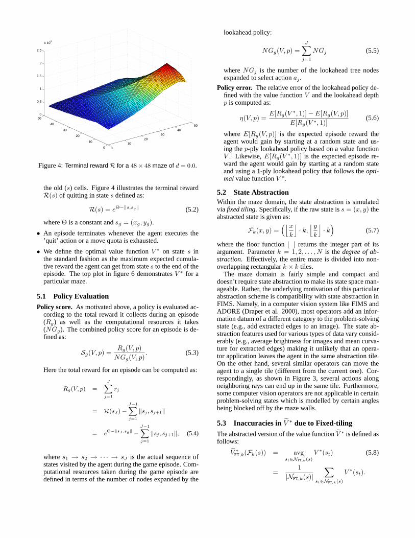
Figure 4:Terminal reward R for a 48× 48 maze of d = 0.0.

the old (s) cells. Figure 4 illustrates the terminal rewardR(s) of quitting in states defined as:

R(s) = eΘ−‖s,sg‖ (5.2)

whereΘ is a constant andsg = (xg, yg).

• An episode terminates whenever the agent executes the’quit’ action or a move quota is exhausted.

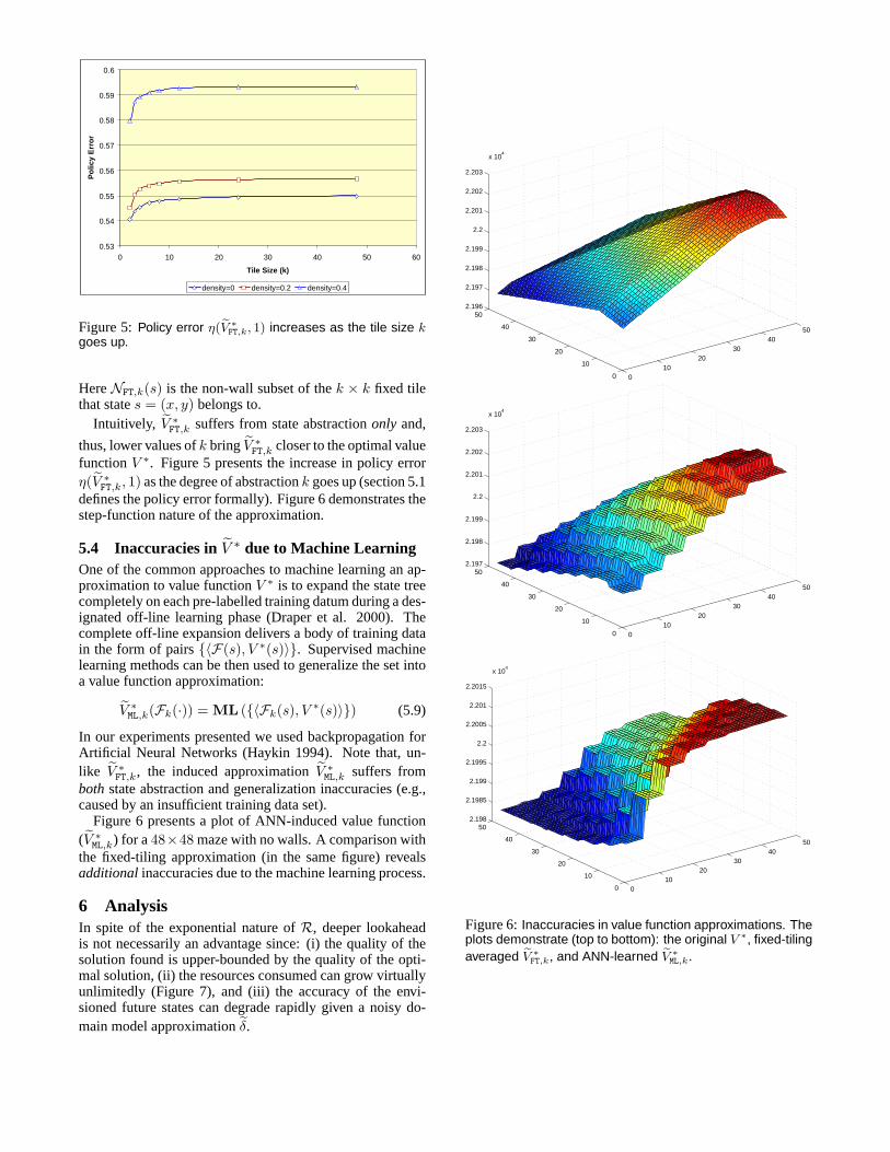
• We define the optimal value functionV ∗ on states inthe standard fashion as the maximum expected cumula-tive reward the agent can get from states to the end of theepisode. The top plot in figure 6 demonstratesV ∗ for aparticular maze.

5.1 Policy EvaluationPolicy score. As motivated above, a policy is evaluated ac-

cording to the total reward it collects during an episode(Rg) as well as the computational resources it takes(NGg). The combined policy score for an episode is de-fined as:

Sg(V, p) =Rg(V, p)

NGg(V, p). (5.3)

Here the total reward for an episode can be computed as:

Rg(V, p) =

J∑j=1

rj

= R(sJ)−J−1∑j=1

‖sj , sj+1‖

= eΘ−‖sJ ,sg‖ −J−1∑j=1

‖sj , sj+1‖, (5.4)

wheres1 → s2 → · · · → sJ is the actual sequence ofstates visited by the agent during the game episode. Com-putational resources taken during the game episode aredefined in terms of the number of nodes expanded by the

lookahead policy:

NGg(V, p) =J∑

j=1

NGj (5.5)

whereNGj is the number of the lookahead tree nodesexpanded to select actionaj .

Policy error. The relative error of the lookahead policy de-fined with the value functionV and the lookahead depthp is computed as:

η(V, p) =E[Rg(V ∗, 1)]− E[Rg(V, p)]

E[Rg(V ∗, 1)](5.6)

where E[Rg(V, p)] is the expected episode reward theagent would gain by starting at a random state and us-ing thep-ply lookahead policy based on a value functionV . Likewise, E[Rg(V ∗, 1)] is the expected episode re-ward the agent would gain by starting at a random stateand using a 1-ply lookahead policy that follows theopti-malvalue functionV ∗.

5.2 State AbstractionWithin the maze domain, the state abstraction is simulatedvia fixed tiling. Specifically, if the raw state iss = (x, y) theabstracted state is given as:

Fk(x, y) =(⌊x

k

⌋· k,

⌊y

k

⌋· k

)(5.7)

where the floor functionb c returns the integer part of itsargument. Parameterk = 1, 2, . . . , N is thedegree of ab-straction. Effectively, the entire maze is divided into non-overlapping rectangulark × k tiles.

The maze domain is fairly simple and compact anddoesn’t require state abstraction to make its state space man-ageable. Rather, the underlying motivation of this particularabstraction scheme is compatibility with state abstraction inFIMS. Namely, in a computer vision system like FIMS andADORE (Draper et al. 2000), most operators add an infor-mation datum of a different category to the problem-solvingstate (e.g., add extracted edges to an image). The state ab-straction features used for various types of data vary consid-erably (e.g., average brightness for images and mean curva-ture for extracted edges) making it unlikely that an opera-tor application leaves the agent in the same abstraction tile.On the other hand, several similar operators can move theagent to a single tile (different from the current one). Cor-respondingly, as shown in Figure 3, several actions alongneighboring rays can end up in the same tile. Furthermore,some computer vision operators are not applicable in certainproblem-solving states which is modelled by certain anglesbeing blocked off by the maze walls.

5.3 Inaccuracies inV ∗ due to Fixed-tilingThe abstracted version of the value functionV ∗ is defined asfollows:

V ∗FT,k(Fk(s)) = avg

st∈NFT,k(s)

V ∗(st) (5.8)

=1

|NFT,k(s)|∑

st∈NFT,k(s)

V ∗(st).

0.53

0.54

0.55

0.56

0.57

0.58

0.59

0.6

0 10 20 30 40 50 60

Tile Size (k)

Po

licy

Err

or

density=0 density=0.2 density=0.4

Figure 5:Policy error η(V ∗FT,k, 1) increases as the tile size k

goes up.

HereNFT,k(s) is the non-wall subset of thek × k fixed tilethat states = (x, y) belongs to.

Intuitively, V ∗FT,k suffers from state abstractiononly and,

thus, lower values ofk bringV ∗FT,k closer to the optimal value

functionV ∗. Figure 5 presents the increase in policy errorη(V ∗

FT,k, 1) as the degree of abstractionk goes up (section 5.1defines the policy error formally). Figure 6 demonstrates thestep-function nature of the approximation.

5.4 Inaccuracies inV ∗ due to Machine LearningOne of the common approaches to machine learning an ap-proximation to value functionV ∗ is to expand the state treecompletely on each pre-labelled training datum during a des-ignated off-line learning phase (Draper et al. 2000). Thecomplete off-line expansion delivers a body of training datain the form of pairs{〈F(s), V ∗(s)〉}. Supervised machinelearning methods can be then used to generalize the set intoa value function approximation:

V ∗ML,k(Fk(·)) = ML ({〈Fk(s), V ∗(s)〉}) (5.9)

In our experiments presented we used backpropagation forArtificial Neural Networks (Haykin 1994). Note that, un-like V ∗

FT,k, the induced approximationV ∗ML,k suffers from

both state abstraction and generalization inaccuracies (e.g.,caused by an insufficient training data set).

Figure 6 presents a plot of ANN-induced value function(V ∗

ML,k) for a48×48 maze with no walls. A comparison withthe fixed-tiling approximation (in the same figure) revealsadditionalinaccuracies due to the machine learning process.

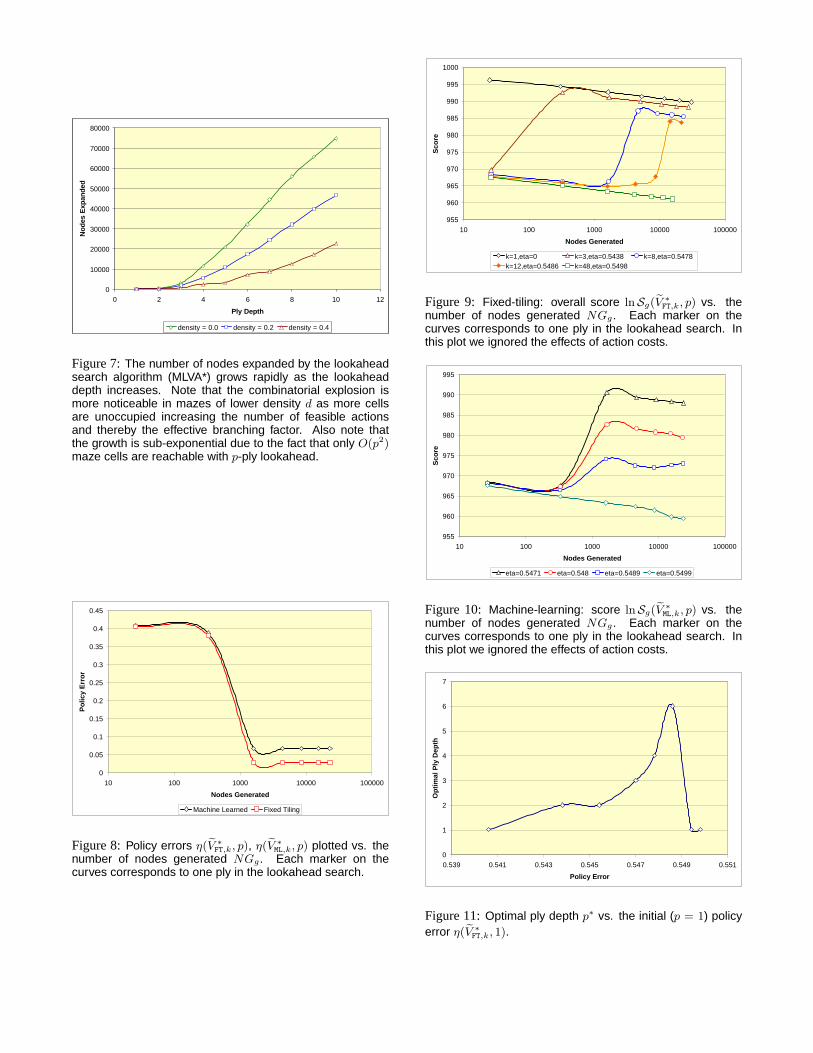
6 AnalysisIn spite of the exponential nature ofR, deeper lookaheadis not necessarily an advantage since: (i) the quality of thesolution found is upper-bounded by the quality of the opti-mal solution, (ii) the resources consumed can grow virtuallyunlimitedly (Figure 7), and (iii) the accuracy of the envi-sioned future states can degrade rapidly given a noisy do-main model approximationδ.

010

2030

4050

0

10

20

30

40

502.196

2.197

2.198

2.199

2.2

2.201

2.202

2.203

x 104

010

2030

4050

0

10

20

30

40

502.197

2.198

2.199

2.2

2.201

2.202

2.203

x 104

010

2030

4050

0

10

20

30

40

502.198

2.1985

2.199

2.1995

2.2

2.2005

2.201

2.2015

x 104

Figure 6:Inaccuracies in value function approximations. Theplots demonstrate (top to bottom): the original V ∗, fixed-tilingaveraged V ∗

FT,k, and ANN-learned V ∗ML,k.

0

10000

20000

30000

40000

50000

60000

70000

80000

0 2 4 6 8 10 12

Ply Depth

Nod

es E

xpan

ded

density = 0.0 density = 0.2 density = 0.4

Figure 7:The number of nodes expanded by the lookaheadsearch algorithm (MLVA*) grows rapidly as the lookaheaddepth increases. Note that the combinatorial explosion ismore noticeable in mazes of lower density d as more cellsare unoccupied increasing the number of feasible actionsand thereby the effective branching factor. Also note thatthe growth is sub-exponential due to the fact that only O(p2)maze cells are reachable with p-ply lookahead.

0

0.05

0.1

0.15

0.2

0.25

0.3

0.35

0.4

0.45

10 100 1000 10000 100000

Nodes Generated

Po

licy

Err

or

Machine Learned Fixed Tiling

Figure 8:Policy errors η(V ∗FT,k, p), η(V ∗

ML,k, p) plotted vs. thenumber of nodes generated NGg. Each marker on thecurves corresponds to one ply in the lookahead search.

955

960

965

970

975

980

985

990

995

1000

10 100 1000 10000 100000

Nodes Generated

Sco

re

k=1,eta=0 k=3,eta=0.5438 k=8,eta=0.5478k=12,eta=0.5486 k=48,eta=0.5498

Figure 9: Fixed-tiling: overall score lnSg(V ∗FT,k, p) vs. the

number of nodes generated NGg. Each marker on thecurves corresponds to one ply in the lookahead search. Inthis plot we ignored the effects of action costs.

955

960

965

970

975

980

985

990

995

10 100 1000 10000 100000

Nodes Generated

Sco

re

eta=0.5471 eta=0.548 eta=0.5489 eta=0.5499

Figure 10: Machine-learning: score lnSg(V ∗ML,k, p) vs. the

number of nodes generated NGg. Each marker on thecurves corresponds to one ply in the lookahead search. Inthis plot we ignored the effects of action costs.

0

1

2

3

4

5

6

7

0.539 0.541 0.543 0.545 0.547 0.549 0.551

Policy Error

Op

tim

al P

ly D

epth

Figure 11:Optimal ply depth p∗ vs. the initial (p = 1) policyerror η(V ∗

FT,k, 1).

We are currently working on an analytical study of theempirical evidence. Preliminary results are as follows:

1. As expected, lookahead reduces the policy error. Figure8 presents the empirical results for the policies guidedby a fixed-tiling abstracted approximationV ∗

FT,k and a

machine-learned approximationV ∗ML,k.

2. Lookahead initially improves overall policy performancein the presence ofinadmissiblevalue function inaccu-racies induced bystate abstractionor machine learning(Figures 9 and 10). While deeper values of lookahead dodecrease the policy error (Figure 8) they also result in thelarger numbers of nodes expanded (Figure 7) thereby ad-versely affecting the overall score.

3. The optimal lookahead search horizon (p∗) is reachedfairly rapidly. Figure 11 presents the empirical results fora fixed-tile approximation toV ∗. Note, as the value func-tion approximationV ∗

FT,k becomes progressively more in-

accurate (i.e., its policy errorη(V ∗FT,k, 1) increases), the

optimal ply depth decreases again partly due to the com-binatorial explosion ofNGg.

4. Remarkably, the nature of ANN-induced inaccuracies inV ∗ML,k, doesnot call for deeper lookahead as the policy

error increases. Indeed, figure 10 demonstrates that thebest score is always reached atp∗ = 3 regardless of theinitial η(V ∗

ML,k, p). The attributes ofV ∗ML,k leading to this

phenomenon are yet to be better characterized.

7 Related WorkAs our evaluation criteria depends on both the quality of theoutcome, and the computational time required, it is clearlyrelated to ”type II optimality” (Good 1971), ”limited ratio-nality” (Russell et al. 1991), and ”meta-greedy optimiza-tion” (Russell et al. 1993; Isukapalli et al. 2001). Our re-sults differ as we are considering a different task (depth ofsearch in the context of an image interpretation task), and weare isolating the problem of adaptively selecting the optimallookahead depth.

7.1 ADOREAdaptive image recognition system ADORE (Draper et al.2000) is a well-known MDP-based control policy imple-mentations in computer vision. The FIMS prototype canbe considered as a testbed for several significant extensionsover ADORE. The extension most relevant to this paperis the emphasis on internal lookahead. In other words,ADORE selects operators in a greedy (i.e., the lookaheadof depth 1) fashion guided by its MDP value function. As aresult, the existing inaccuracies in the value function causedby state abstraction or machine learning deficiencies, oftenforce ADORE to undo its actions and backtrack. On theother hand, FIMS attempts to predict effects ofaction se-quencesand is expected to be less sensitive to value functioninaccuracies.

7.2 Minimax and MiniminMost board game-playing programs use a lookahead search.In particular, the first computer program to ever win a

man-machine world championship, Chinook (Schaeffer etal. 1992), and the first system to defeat the human world-champion in chess, Deep Blue (Hsu et al. 1995) utilizeda minimax-based lookahead search. Like FIMS, they com-pensate for the insensitivity ofV ∗ via envisioning the fu-ture states many plies ahead. The core differences betweenminimax and minimin (Korf 1990) algorithms and FIMS in-clude minimax’s easily recognizable goal states, perfect do-main modelδ, fully deterministic actions, and the use of fullunabstracted states for the lookahead. Additionally, somealgorithms (e.g., branch and bound or minimax with alphapruning) leave out entire search subtrees by assuming an ad-missible heuristic function which is unavailable in FIMS.An interesting study of minimax pathologies is presented in(Nau 1983).

7.3 MinervaReal-time ship-board damage control system Minerva (Bu-litko 1998) demonstrated a 318% improvement over humansubject matter experts and was successfully deployed in theUS Navy. It selects actions dynamically using an approx-imate Petri Nets based domain model (δ) and a machine-learned decision-tree-based value function (V ∗). The keydistinctions between Minerva and FIMS include a fixedlookahead depth and fixed state abstraction features used forenvisionment. Therefore, the focus of this paper – the in-terplay between the lookahead depth and the degree of stateabstraction – is not considered in the research on Minerva.

8 Summary and Future ResearchThis paper describes the practical challenges of produc-ing an efficient and accurate image interpretation system(FIMS). We first indicate why this corresponds to a Markovdecision process, as we apply asequenceof operators to gofrom raw images to an interpretation, and moreover must de-cide on the appropriate operatordynamically, based on theactual state.

At each stage, FIMS uses a real-time best-first search todetermine which operator to apply. Due to the size of indi-vidual states, FIMS actually usesabstractionsof the states,rather than the states themselves making the entire processPOMDP. The heuristic value function, used to evaluate thequality of the predicted states, depends on the correctnessof the final interpretation; as FIMS is dealing with novelimages, this information is not immediately available. In-stead, we first learn an approximation to this heuristic func-tion given a small set of pre-labelled training images. In ad-dition, as FIMS must select the appropriate operator quickly,we want a search process that is both accurate and efficient.

This paper investigates the effectiveness of the lookaheadpolicy given these challenges. In particular, we take a steptowards determining, automatically, the appropriate looka-head depth we should use, as a function of inaccuracies dueto the state abstractions as well as the machine-learned es-timates of the heuristic, with respect to our specific ”type IIoptimality”. Applications of this research range from time-constrained game playing and path-finding to real-time im-age interpretation and ship-board damage control.

The empirical study in a FIMS-compatible variant of thegrid world testbed gives us a better understanding of the fine

interplay between various factors affecting performance of alookahead best-first control policy. It therefore sets the stagefor developing a theory and an implementation of a dynamicand automated lookahead depth selection module. One ofthe immediate open questions is the relation between inac-curacies in theapproximatedomain modelδ, the approxi-mate value functionV ∗, and the optimal lookahead searchdepth. Likewise, better understanding of the optimal looka-head depth in the presence of machine-learning inaccuraciesis needed.

AcknowledgementsGuanwen Zhang and Ying Yuang have assisted with the de-velopment of the maze domain environment at the Univer-sity of Alberta. We thank Terry Caelli, Omid Madani, andAlberta Research Council staff for an insightful input andversatile support. The paper also benefited from the com-ments by anonymous reviewers. Finally, we are grateful tothe funding from the University of Alberta and NSERC.

ReferencesBulitko, V. 1998. Minerva-5: A Multifunctional Dynamic Ex-pert System.MS Thesis. Department of CS, Univ. of Illinois atUrbana-Champaign.

Cheng, L., Caelli, T., Bulitko, V. 2002. Image Annotation UsingProbabilistic Evidence Prototyping Methods.International Jour-nal of Pattern Recognition and Artificial Intelligence. (in prepara-tion).

Draper, B., Bins, J., Baek, K. 2000. ADORE: Adaptive ObjectRecognition,Videre, 1(4):86–99.

Good, I.J. 1971. Twenty-seven Principles of Rationality. InFoun-dations of Statistical Inference, Godambe V.P., Sprott, D.A. (edi-tors), Holt, Rinehart and Winston, Toronto.

Gougeon, F.A. 1993. Individual Tree Identification from HighResolution MEIS Images,In Proceedings of the International Fo-rum on Airborne Multispectral Scanning for Forestry and Map-ping, Leckie, D.G., and Gillis, M.D. (editors), pp. 117-128.

Haykin, S. 1994.Neural Networks: A Comprehensive Founda-tion. Macmillian College Pub. Co.

Hsu, F.H., Campbell, M.S., Hoane, A.J.J. 1995. Deep Blue Sys-tem Overview.Proceedings of the 9th ACM Int. Conf. on Super-computing, pp. 240-244.

Isukapalli, R., Greiner, R. 2001. Efficient Interpretation Policies,Proceedings of IJCAI’01, pp. 1381–1387.

Korf, R.E. 1990. Real-time heuristic search.Artificial Intelli-gence, Vol. 42, No. 2-3, pp. 189-211.

Larsen, M. and Rudemo, M. 1997. Using ray-traced templates tofind individual trees in aerial photos.In Proceedings of the 10thScandinavian Conference on Image Analysis, volume 2, pages1007-1014.

Nau, D.S. 1983. Pathology on Game Trees Revisited, and an Al-ternative to Minimaxing.Artificial Intelligence, 21(1, 2):221-244.

Newborn, M. 1997.Kasparov vs. Deep Blue: Computer ChessComes Out of Age. Springer-Verlag.

Pollock, R.J. 1994. A Model-based Approach to AutomaticallyLocating Tree Crowns in High Spatial Resolution Images.Imageand Signal Processing for Remote Sensing. Jacky Desachy, editor.

Russell, S., Wefald, E. 1991.Do the right thing : studies in limitedrationality. Artificial Intelligence series, MIT Press, Cambridge,Mass.

Russell, S., Subramanian, D., Parr, R. 1993. Provably BoundedOptimal Agents.Proceedings of IJCAI’93.

Schaeffer, J., Culberson, J., Treloar, N., Knight, B., Lu, P.,Szafron, D. 1992. A World Championship Caliber Checkers Pro-gram.Artificial Intelligence, Volume 53, Number 2-3, pages 273-290.

Sutton, R.S., Barto, A.G., 2000.Reinforcement Learning: An In-troduction. MIT Press.