ECE 5655/4655 Real-Time DSP 7–1 Real-Time FIR Digital Filters Introduction Digital filter design techniques fall into either finite impulse response (FIR) or infinite impulse response (IIR) approaches. In this chapter we are concerned with just FIR designs. We will start with an overview of general digital filter design, but the emphasis of this chapter will be on real-time implementation of FIR filters using C and assembly. • Basic FIR filter topologies will be reviewed • To motivate the discussion of real-time implementation we will begin with a brief overview of FIR filter design • Both fixed and floating-point implementations will be con- sidered – The MATLAB signal processing toolbox and filter design toolbox will be used to create quantized filter coefficients • The use of circular addressing in assemble will be considered • Implementing real-time filtering using analog I/O will be implemented using the AIC23 codec interface and associated ISR routines Chapter 7

Welcome message from author
This document is posted to help you gain knowledge. Please leave a comment to let me know what you think about it! Share it to your friends and learn new things together.
Transcript

er
Real-Time FIR Digital FiltersIntroduction
Digital filter design techniques fall into either finite impulseresponse (FIR) or infinite impulse response (IIR) approaches. Inthis chapter we are concerned with just FIR designs. We will startwith an overview of general digital filter design, but the emphasisof this chapter will be on real-time implementation of FIR filtersusing C and assembly.
• Basic FIR filter topologies will be reviewed
• To motivate the discussion of real-time implementation wewill begin with a brief overview of FIR filter design
• Both fixed and floating-point implementations will be con-sidered
– The MATLAB signal processing toolbox and filter designtoolbox will be used to create quantized filter coefficients
• The use of circular addressing in assemble will be considered
• Implementing real-time filtering using analog I/O will beimplemented using the AIC23 codec interface and associatedISR routines
Chapt
7
ECE 5655/4655 Real-Time DSP 7–1
Chapter 7 • Real-Time FIR Digital Filters
Basics of Digital Filter Design
• A filter is a frequency selective linear time invariant (LTI)system, that is a system that passes specified frequency com-ponents and rejects others
• The discrete-time filter realizations of interest here are thoseLTI systems which have LCCDE representation and arecausal
• Note that for certain applications noncausal filters are appro-priate
• An important foundation for digital filter design are the clas-sical analog filter approximations
• The filter design problem can be grouped into three stages:
– Specification of the desired system properties (applicationdriven)
– Approximation of the specifications using causal discrete-time systems
– System realization (technology driven - hardware/soft-ware)
7–2 ECE 5655/4655 Real-Time DSP

Basics of Digital Filter Design
• A common scenario in which one finds a digital filter is in thefiltering of a continuous-time signal using an A/D- -D/Asystem
• Strictly speaking is a discrete-time filter although it iscommonly referred to as a digital filter
• Recall that for the continuous-time system described above(ideally)
(7.1)
• Using the change of variables , where is the sam-ple spacing, we can easily convert continuous-time specifica-tions to discrete-time specifications i.e.,
(7.2)
H z
Discrete-Time
SystemC/D D/C
TT
xa t ya t x n y n
H z
Heff j H ejT , T
0, otherwise
=
T= T
H ej Heff j
T----
=
ECE 5655/4655 Real-Time DSP 7–3

Chapter 7 • Real-Time FIR Digital Filters
Overview of Approximation Techniques
• Digital filter design techniques fall into either IIR or FIRapproaches
• General Approximation Approaches:
– Placement of poles and zeros (ad-hoc)
– Numerical solution of differential equations
– Impulse invariant (step invariant etc.)
– Bilinear transformation
– Minimum mean-square error (frequency domain)
• FIR Approximation Approaches
– Truncated impulse response of ideal brickwall responsesusing window functions
– Frequency sampling desired response using transition sam-ples
– Optimum equiripple approximations (use the Parks-McClellan algorithm via the Remez exchange algorithm,firpm() in MATLAB)
– Minimum mean-square error in the frequency domain
• In the FIR approaches the additional constraint of linearphase is usually imposed
7–4 ECE 5655/4655 Real-Time DSP

Basic FIR Filter Topologies
Basic FIR Filter Topologies
• Recall that a causal FIR filter containing coefficientshas impulse response
(7.3)
• The corresponding z-transform of the filter is
(7.4)
• The frequency response of the filter is
(7.5)
• The classical direct form topology for this filter is shownbelow
• Often times we are dealing with linear phase FIR designswhich have even or odd symmetry, e.g.,
M 1+
h n ak n k– k 0=
M
=
H z akzk–
k 0=
M
a0 a1z1– aM 1– z
M–+ + += =
H ej ake
jk–
k 0=
M
=
z1–
z1–
z1–
a0
y n
x n ...
...a1 a2 aM 1– aM
Direct Form FIR Structure
ECE 5655/4655 Real-Time DSP 7–5
Chapter 7 • Real-Time FIR Digital Filters
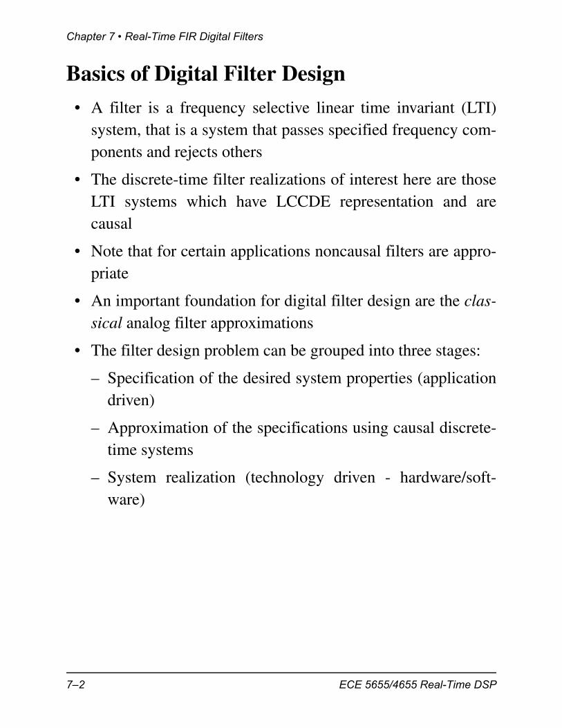
(7.6)
• In this case a more efficient structure, reducing the number ofmultiplications from to , is
• Another structure, not as popular as the first two, is the FIRlattice
– Although not discussed any further here, the reflectioncoefficients, , are related to the via a recurrence for-mula (in MATLAB we use k=tf2latc(num))
h n h M n– even=
h n h M n– odd–=
M 1+ M 2 1+
z1–
z1–
z1–
a0y n
x n ...
...
a1 a2 aM 2 1– aM 2
Modified Direct Form FIR Structure for M Even
z1–
z1–
z1–
z1–
...
FilterCenter
y n x n ...
...FIR Lattice Structure
z1–
z1–
z1–
k1k1
k2k2
kM 1–kM 1–
ki ak
7–6 ECE 5655/4655 Real-Time DSP
Overview of FIR Filter Design
– The lattice structure is very robust under coefficient quan-tization
Overview of FIR Filter Design
Why or Why Not Choose FIR?
• FIR advantages over IIR
– Can be designed to have exactly linear phase
– Typically implemented with nonrecursive structures, thusthey are inherently stable
– Quantization effects can be minimized more easily
• FIR disadvantages over IIR
– A higher filter order is required to obtain the same ampli-tude response compared to a similar IIR design
– The higher filter order also implies higher computationalcomplexity
– The higher order filter also implies greater memoryrequirements for storing coefficients
FIR Design Using Windowing
• The basic approach is founded in the fact that ideal lowpass,highpass, bandpass, and bandstop filters, have the followingnoncausal impulse responses on n –
ECE 5655/4655 Real-Time DSP 7–7
Chapter 7 • Real-Time FIR Digital Filters
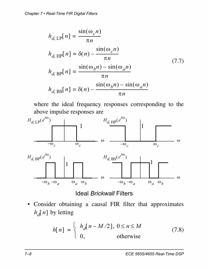
(7.7)
where the ideal frequency responses corresponding to theabove impulse responses are
• Consider obtaining a causal FIR filter that approximates by letting
(7.8)
hd LP n cn sin
n----------------------=
hd HP n n cn sin
n----------------------–=
hd BP n bn sin an sin–
n---------------------------------------------------=
hd BS n n bn sin an sin–
n---------------------------------------------------–=
Hd LP ej
Hd BP ej
Hd BS ej
Hd HP ej
c– c c– c
a b– b a– a b– b a–
Ideal Brickwall Filters
1 1
1 1
hd n
h n hd n M 2– , 0 n M
0, otherwise
=
7–8 ECE 5655/4655 Real-Time DSP
Overview of FIR Filter Design
• Effectively we have applied a rectangular window to and moved the saved portion of the impulse response to theright to insure that for causality, for
– The applied rectangular window can be represented as
(7.9)
where here is unity for and zero otherwise
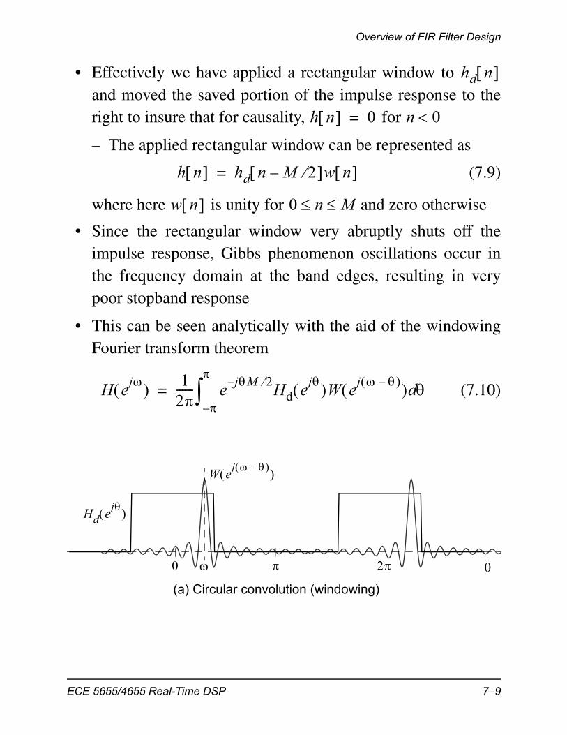
• Since the rectangular window very abruptly shuts off theimpulse response, Gibbs phenomenon oscillations occur inthe frequency domain at the band edges, resulting in verypoor stopband response
• This can be seen analytically with the aid of the windowingFourier transform theorem
(7.10)
hd n
h n 0= n 0
h n hd n M 2– w n =
w n 0 n M
H ej 1
2------ e
jM 2–Hd e
j W ej – d
–
=
2
W ej –
Hd ej
0
(a) Circular convolution (windowing)
ECE 5655/4655 Real-Time DSP 7–9

Chapter 7 • Real-Time FIR Digital Filters
– Use of the rectangular window results in about 9% peakripple in both the stopband and passband; equivalently thepeak passband ripple is 0.75 dB, while the peak sidelobelevel is down only 21 dB
• To both decrease passband ripple and lower the sidelobes, wemay smoothly taper the window to zero at each end
– Windows chosen are typically symmetrical about the cen-ter
– Additionally, to insure linear phase, the complete impulseresponse must be either symmetric or antisymmetric about
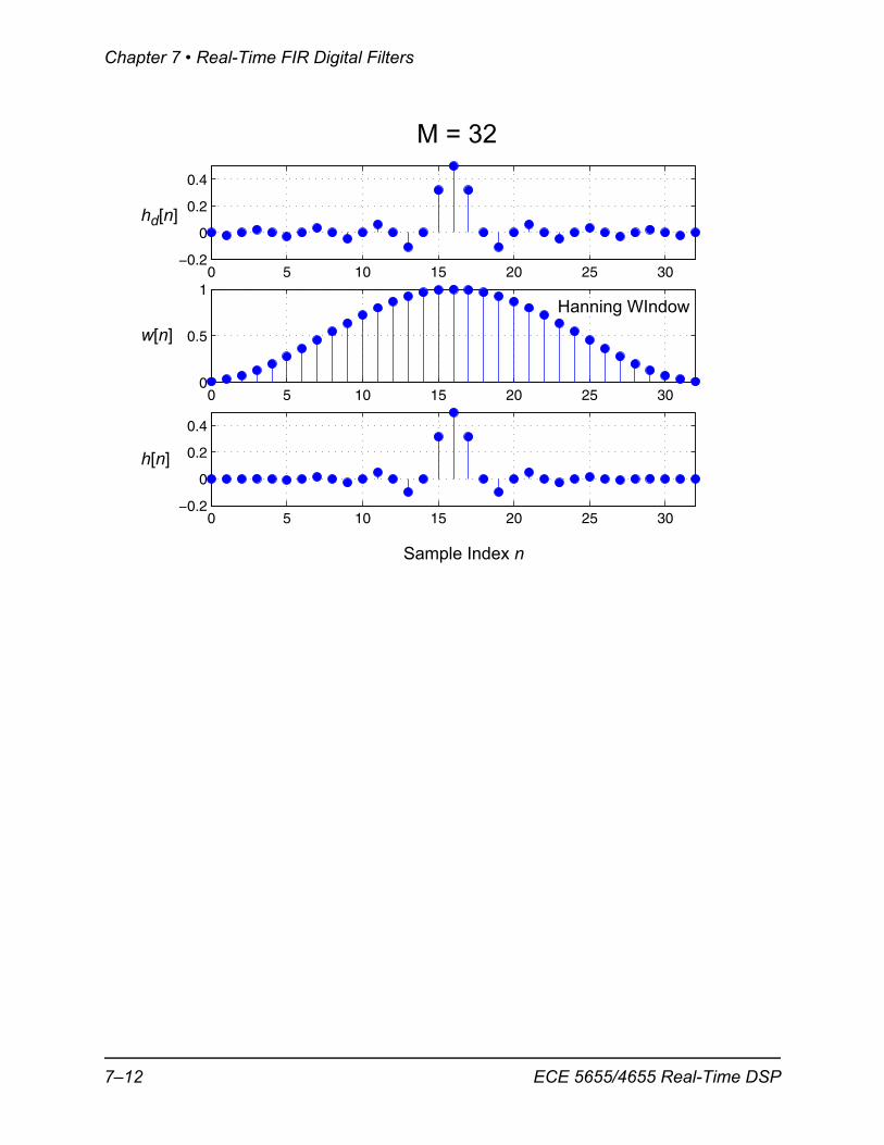
Example: Use of the Hanning Window
• The Hanning window is defined as follows
20
H ej
(b) Resulting frequency response of windowed sinc(x)
M 2
M 2
7–10 ECE 5655/4655 Real-Time DSP
Overview of FIR Filter Design
(7.11)
• Consider an point design with
• The basic response for a lowpass is of the form
(7.12)
since
• Ultimately we will use MATLAB filter design functions, butfor now consider a step-by-step approach:
>> n = 0:32;>> hd = pi/2/pi*sinc(pi/2*(n-32/2)/pi);>> w = hanning(32+1);>> h = hd.*w’;>> [Hd,F] = freqz(hd,1,512,1);>> [W,F] = freqz(w,1,512,1);>> [H,F] = freqz(hd.*w',1,512,1);
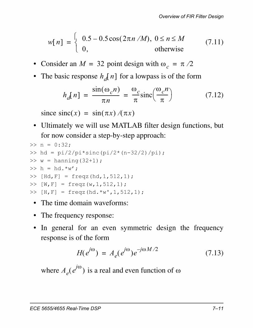
• The time domain waveforms:
• The frequency response:
• In general for an even symmetric design the frequencyresponse is of the form
(7.13)
where is a real and even function of
w n 0.5 0.5 2n M ,cos– 0 n M0, otherwise
=
M 32= c 2=
hd n
hd n cn sin
n----------------------
c
------sinccn
--------- = =
sinc x x sin x =
H ej Ae e
j e jM 2–=
Ae ej
ECE 5655/4655 Real-Time DSP 7–11
Chapter 7 • Real-Time FIR Digital Filters
0 5 10 15 20 25 30−0.2
0
0.2
0.4
0 5 10 15 20 25 300
0.5
1
0 5 10 15 20 25 30−0.2
0
0.2
0.4
Sample Index n
hd[n]
w[n]
h[n]
M = 32
Hanning WIndow
7–12 ECE 5655/4655 Real-Time DSP

Overview of FIR Filter Design
0 0.05 0.1 0.15 0.2 0.25 0.3 0.35 0.4 0.45 0.5−60
−40
−20
0
0 0.05 0.1 0.15 0.2 0.25 0.3 0.35 0.4 0.45 0.5−60−40−20
020
0 0.05 0.1 0.15 0.2 0.25 0.3 0.35 0.4 0.45 0.5−60
−40
−20
0
2------
Hd ej dB
W ej dB
H ej dB
M = 32Down only 21 dB
Hanning WIndow
ECE 5655/4655 Real-Time DSP 7–13
Chapter 7 • Real-Time FIR Digital Filters
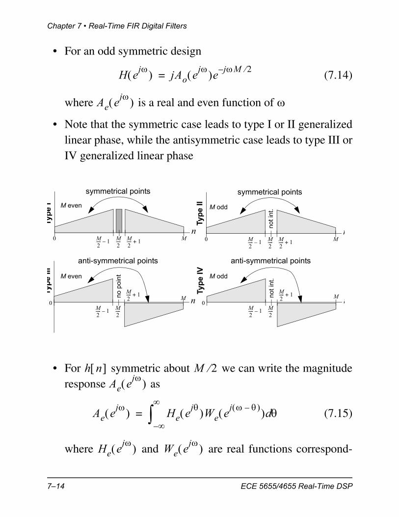
• For an odd symmetric design
(7.14)
where is a real and even function of
• Note that the symmetric case leads to type I or II generalizedlinear phase, while the antisymmetric case leads to type III orIV generalized linear phase
• For symmetric about we can write the magnituderesponse as
(7.15)
where and are real functions correspond-
H ej jAo e
j e jM 2–=
Ae ej
nMM
2----- M
2----- 1+M
2----- 1–0
symmetrical points
Typ
e I
nMM
2----- M
2----- 1+M
2----- 1–0
symmetrical pointsTy
pe
II
nM
M2-----
M2----- 1+
M2----- 1–
0
anti-symmetrical points
Typ
e III
not i
nt.
no p
oin
t
nM
M2-----
M2----- 1+
M2----- 1–
0
anti-symmetrical points
Typ
e IV
not
int.
M even
M even
M odd
M odd
h n M 2Ae e
j
Ae ej He e
j We ej – d
–
=
He ej We e
j
7–14 ECE 5655/4655 Real-Time DSP
Overview of FIR Filter Design
ing to the magnitude responses of the desired filter frequencyresponse and window function frequency response respec-tively
Lowpass Design
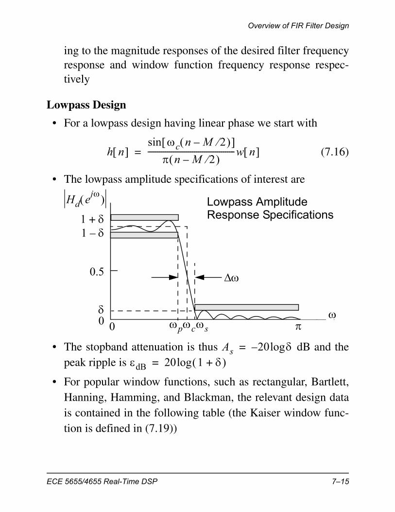
• For a lowpass design having linear phase we start with
(7.16)
• The lowpass amplitude specifications of interest are
• The stopband attenuation is thus dB and thepeak ripple is
• For popular window functions, such as rectangular, Bartlett,Hanning, Hamming, and Blackman, the relevant design datais contained in the following table (the Kaiser window func-tion is defined in (7.19))
h n c n M 2– sin
n M 2– ---------------------------------------------w n =
1 –1 +
0.5
0
pcs
Hd ej Lowpass Amplitude
Response Specifications
0
As 20 log–=dB 20 1 + log=
ECE 5655/4655 Real-Time DSP 7–15

Chapter 7 • Real-Time FIR Digital Filters
The general design steps:
1. Choose the window function, , that just meets the stop-band requirements as given in the Table 7.1
2. Choose the filter length, M, (actual length is ) such that
(7.17)
3. Choose in the truncated impulse response such that
(7.18)
4. Plot to see if the specifications are satisfied5. Adjust and M if necessary to meet the requirements; If pos-
sible reduce M
Table 7.1: Window characteristics for FIR design.
TypeTransition Bandwidth
Minimum Stopband
Attenuation
Equivalent Kaiser
Rectangle 21 dB 0
Bartlett 25 dB 1.33
Hanning 44 dB 3.86
Hamming 53 dB 4.86
Blackman 74 dB 7.04
1.81 M
1.80 M
5.01 M
6.27 M
9.19 M
w n
M 1+
s p–
c
cp s+
2-------------------=
H ej
c
7–16 ECE 5655/4655 Real-Time DSP
Overview of FIR Filter Design
• By using the Kaiser window method some of the trial anderror can be eliminated since via parameter , the stopbandattenuation can be precisely controlled, and then the filterlength for a desired transition bandwidth can be chosen
Kaiser window design steps:
1. Let be a Kaiser window, i.e.,
(7.19)
2. Chose for the specified as
(7.20)
3. The window length M is then chosen to satisfy
(7.21)
4. The value chosen for is chosen as before
w n
w n I0 1n M 2– M
-------------------------2
– 1 2
, 0 n M
0, otherwise
=
As
0.1102 As 8.7– , As 50dB
0.5842 As 21– 0.40.07886 As 21– ,+ 21 As 50
0.0, As 21
=
MAs 8–
2.285 ---------------------=
c
ECE 5655/4655 Real-Time DSP 7–17
Chapter 7 • Real-Time FIR Digital Filters
Optimum Approximations of FIR Filters
• The window method is simple yet limiting, since we cannotobtain individual control over the approximation errors ineach band
• The optimum FIR approach can be applied to type I, II, III,and IV generalized linear phase filters
• The basic idea is to minimize the weighted error between thedesired response and the actual response
(7.22)
• The classical algorithm for performing this minimization inan equiripple sense, was developed by Parks and McClellanin 1972
– Equiripple means that equal amplitude error fluctuationsare introduced in the minimization process
– In MATLAB the associated function is firpm()
• Efficient implementation of the Parks McClellan algorithmrequires the use of the Remez exchange algorithm
• For a detailed development of this algorithm see Oppenheimand Schafer1
• Multiple pass- and stopbands are permitted with this designformulation
1.A. Oppenheim and R. Schafer, Discrete-Time Signal Processing, secondedition, Prentice Hall, Upper Saddle River, New Jersey, 1999.
Hd ej H e
j
E W H ej Hd e
j – =
7–18 ECE 5655/4655 Real-Time DSP
Overview of FIR Filter Design
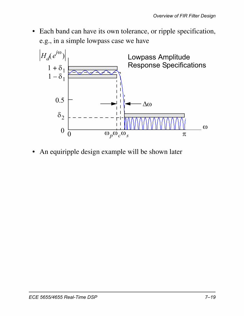
• Each band can have its own tolerance, or ripple specification,e.g., in a simple lowpass case we have
• An equiripple design example will be shown later
1 1–1 1+
0.5
0
2
pcs
Hd ej Lowpass Amplitude
Response Specifications
0
ECE 5655/4655 Real-Time DSP 7–19
Chapter 7 • Real-Time FIR Digital Filters
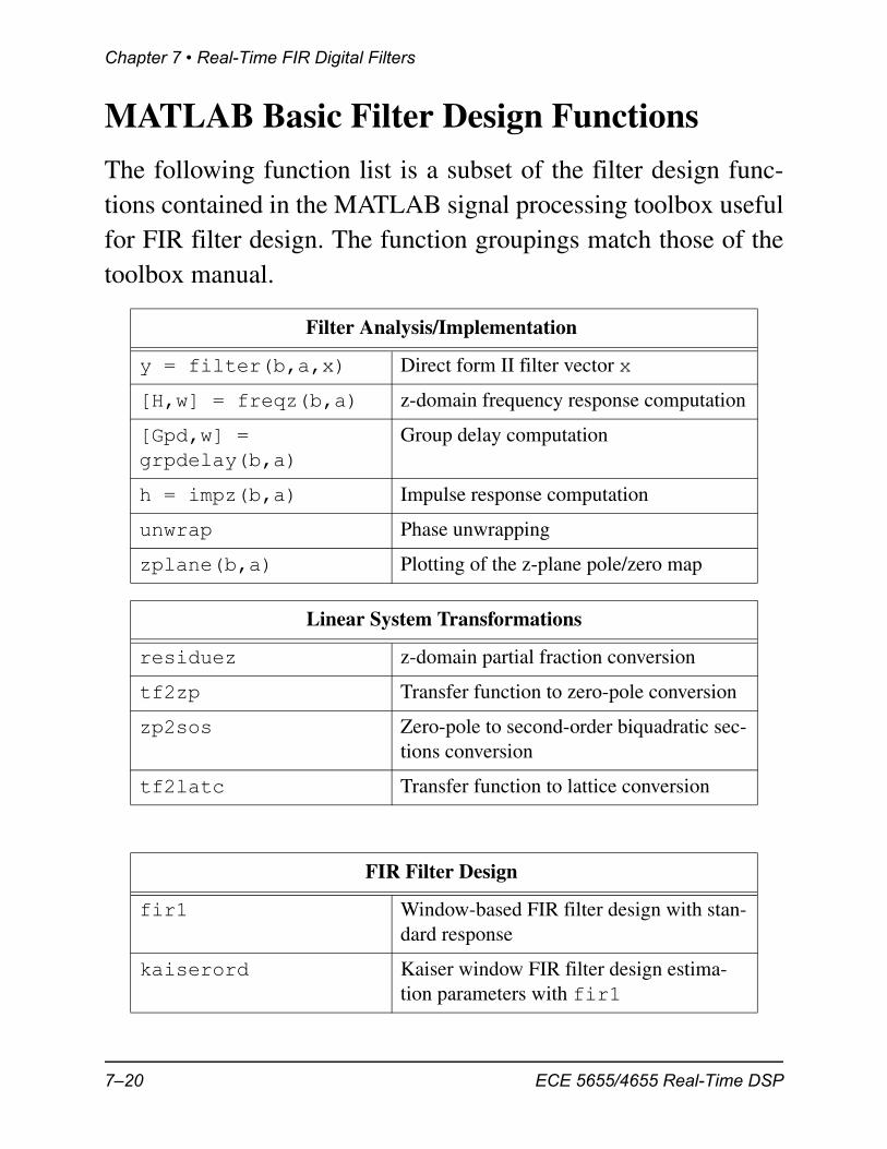
MATLAB Basic Filter Design Functions
The following function list is a subset of the filter design func-tions contained in the MATLAB signal processing toolbox usefulfor FIR filter design. The function groupings match those of thetoolbox manual.
Filter Analysis/Implementation
y = filter(b,a,x) Direct form II filter vector x
[H,w] = freqz(b,a) z-domain frequency response computation
[Gpd,w] = grpdelay(b,a)
Group delay computation
h = impz(b,a) Impulse response computation
unwrap Phase unwrapping
zplane(b,a) Plotting of the z-plane pole/zero map
Linear System Transformations
residuez z-domain partial fraction conversion
tf2zp Transfer function to zero-pole conversion
zp2sos Zero-pole to second-order biquadratic sec-tions conversion
tf2latc Transfer function to lattice conversion
FIR Filter Design
fir1 Window-based FIR filter design with stan-dard response
kaiserord Kaiser window FIR filter design estima-tion parameters with fir1
7–20 ECE 5655/4655 Real-Time DSP
MATLAB Basic Filter Design Functions
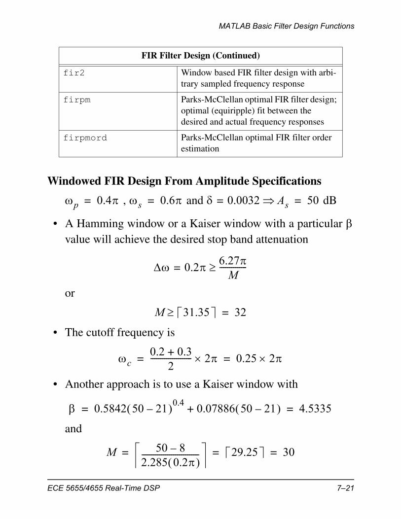
Windowed FIR Design From Amplitude Specifications
, and dB
• A Hamming window or a Kaiser window with a particular value will achieve the desired stop band attenuation
or
• The cutoff frequency is
• Another approach is to use a Kaiser window with
and
fir2 Window based FIR filter design with arbi-trary sampled frequency response
firpm Parks-McClellan optimal FIR filter design; optimal (equiripple) fit between the desired and actual frequency responses
firpmord Parks-McClellan optimal FIR filter order estimation
FIR Filter Design (Continued)
p 0.4= s 0.6= 0.0032= As 50=
0.2=6.27M
--------------
M 31.35 32=
c0.2 0.3+
2--------------------- 2 0.25 2= =
0.5842 50 21– 0.40.07886 50 21– + 4.5335= =
M 50 8–2.285 0.2 ----------------------------- 29.25 30= = =
ECE 5655/4655 Real-Time DSP 7–21
Chapter 7 • Real-Time FIR Digital Filters
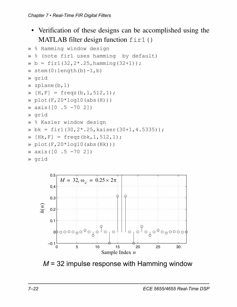
• Verification of these designs can be accomplished using theMATLAB filter design function fir1()
» % Hamming window design» % (note fir1 uses hamming by default)» b = fir1(32,2*.25,hamming(32+1));» stem(0:length(b)-1,b)» grid» zplane(b,1)» [H,F] = freqz(b,1,512,1);» plot(F,20*log10(abs(H)))» axis([0 .5 -70 2])» grid» % Kasier window design» bk = fir1(30,2*.25,kaiser(30+1,4.5335));» [Hk,F] = freqz(bk,1,512,1);» plot(F,20*log10(abs(Hk)))» axis([0 .5 -70 2])» grid
0 5 10 15 20 25 30−0.1
0
0.1
0.2
0.3
0.4
0.5
hn
Sample Index n
M 32 c 0.25 2= =
M = 32 impulse response with Hamming window
7–22 ECE 5655/4655 Real-Time DSP
MATLAB Basic Filter Design Functions
−1 −0.5 0 0.5 1 1.5
−1
−0.5
0
0.5
1
Real Part
Imag
inar
y P
art
32
Note: There are fewmisplaced zeros in this plot due to MATLAB’s problemfinding the rootsof a large polynomial.
Note: The many zeroquadruplets that appear in this linearphase design.
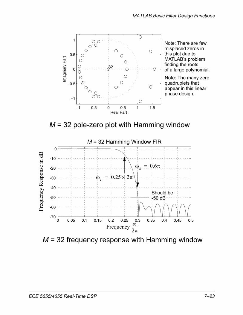
M = 32 pole-zero plot with Hamming window
Frequency 2------
Fre
quen
cy R
espo
nse
in d
B
0 0.05 0.1 0.15 0.2 0.25 0.3 0.35 0.4 0.45 0.5-70
-60
-50
-40
-30
-20
-10
0
s 0.6=
Should be-50 dB
M = 32 Hamming Window FIR
c 0.25 2=
M = 32 frequency response with Hamming window
ECE 5655/4655 Real-Time DSP 7–23
Chapter 7 • Real-Time FIR Digital Filters
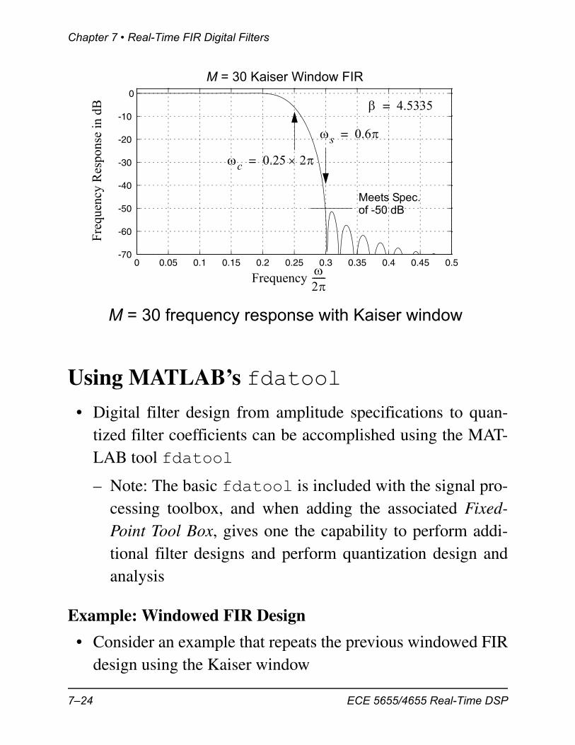
Using MATLAB’s fdatool
• Digital filter design from amplitude specifications to quan-tized filter coefficients can be accomplished using the MAT-LAB tool fdatool
– Note: The basic fdatool is included with the signal pro-cessing toolbox, and when adding the associated Fixed-Point Tool Box, gives one the capability to perform addi-tional filter designs and perform quantization design andanalysis
Example: Windowed FIR Design
• Consider an example that repeats the previous windowed FIRdesign using the Kaiser window
0 0.05 0.1 0.15 0.2 0.25 0.3 0.35 0.4 0.45 0.5-70
-60
-50
-40
-30
-20
-10
0
Frequency 2------
Fre
quen
cy R
espo
nse
in d
B
s 0.6=
Meets Spec.of -50 dB
M = 30 Kaiser Window FIR
c 0.25 2=
4.5335=
M = 30 frequency response with Kaiser window
7–24 ECE 5655/4655 Real-Time DSP
Using MATLAB’s fdatool
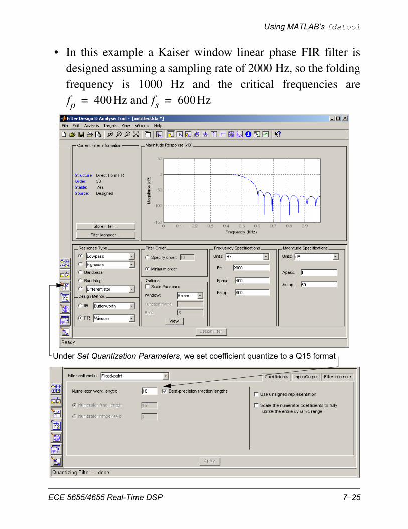
• In this example a Kaiser window linear phase FIR filter isdesigned assuming a sampling rate of 2000 Hz, so the foldingfrequency is 1000 Hz and the critical frequencies are
Hz and Hzfp 400= fs 600=
Under Set Quantization Parameters, we set coefficient quantize to a Q15 format
ECE 5655/4655 Real-Time DSP 7–25

Chapter 7 • Real-Time FIR Digital Filters
• Many other filter viewing options are available as well
– Display phase, Gain & phase, Group delay
– Impulse response, Step response
– Pole-zero plot
– Filter coefficients
• Once you are satisfied with a design, the filter coefficientscan be exported to a .h file, or to the MATLAB workspace
7–26 ECE 5655/4655 Real-Time DSP
Using MATLAB’s fdatool
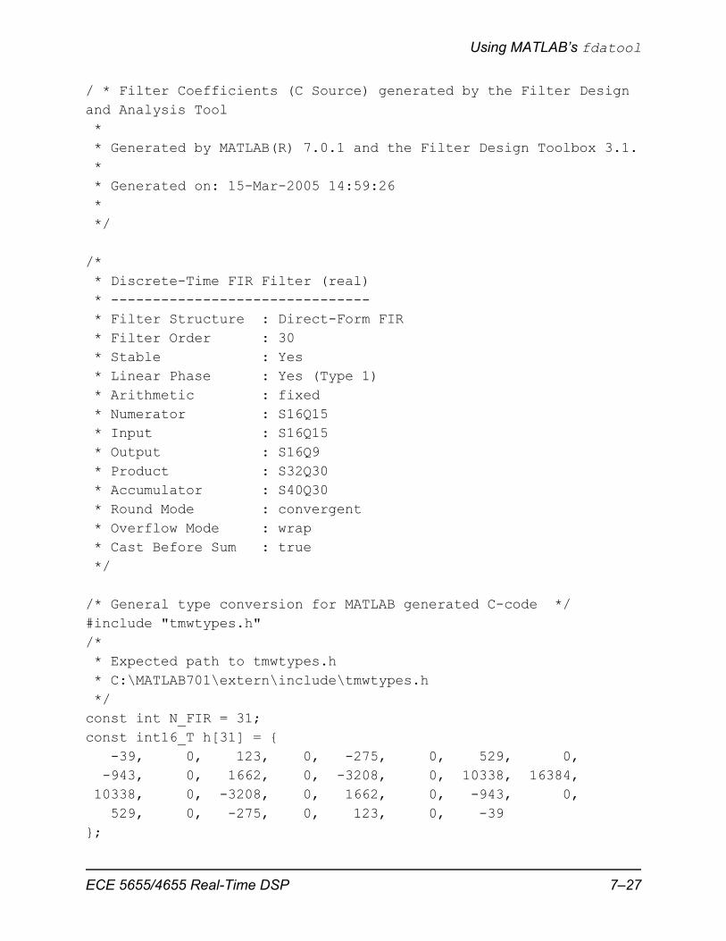
/ * Filter Coefficients (C Source) generated by the Filter Design and Analysis Tool * * Generated by MATLAB(R) 7.0.1 and the Filter Design Toolbox 3.1. * * Generated on: 15-Mar-2005 14:59:26 * */
/* * Discrete-Time FIR Filter (real) * ------------------------------- * Filter Structure : Direct-Form FIR * Filter Order : 30 * Stable : Yes * Linear Phase : Yes (Type 1) * Arithmetic : fixed * Numerator : S16Q15 * Input : S16Q15 * Output : S16Q9 * Product : S32Q30 * Accumulator : S40Q30 * Round Mode : convergent * Overflow Mode : wrap * Cast Before Sum : true */
/* General type conversion for MATLAB generated C-code */#include "tmwtypes.h"/* * Expected path to tmwtypes.h * C:\MATLAB701\extern\include\tmwtypes.h */const int N_FIR = 31;const int16_T h[31] = { -39, 0, 123, 0, -275, 0, 529, 0, -943, 0, 1662, 0, -3208, 0, 10338, 16384, 10338, 0, -3208, 0, 1662, 0, -943, 0, 529, 0, -275, 0, 123, 0, -39};
ECE 5655/4655 Real-Time DSP 7–27
Chapter 7 • Real-Time FIR Digital Filters
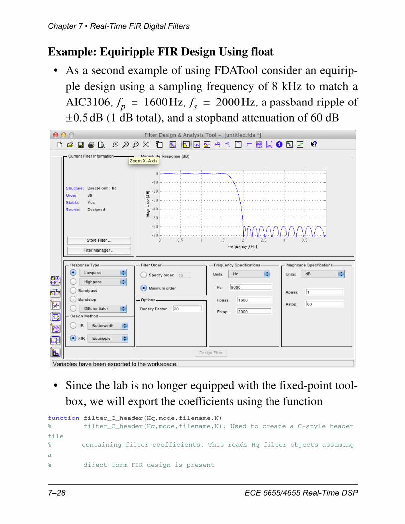
Example: Equiripple FIR Design Using float
• As a second example of using FDATool consider an equirip-ple design using a sampling frequency of 8 kHz to match aAIC3106, Hz, Hz, a passband ripple of
dB (1 dB total), and a stopband attenuation of 60 dB
• Since the lab is no longer equipped with the fixed-point tool-box, we will export the coefficients using the function
function filter_C_header(Hq,mode,filename,N)% filter_C_header(Hq,mode,filename,N): Used to create a C-style header
file% containing filter coefficients. This reads Hq filter objects assuming
a
% direct-form FIR design is present
fp 1600= fs 2000=0.5
7–28 ECE 5655/4655 Real-Time DSP

Using MATLAB’s fdatool
%
% Hq = quantized filter object containing desired coefficients
% mode = specify 'fixed', 'float', or 'exponent'
% file_name = string name of file to be created
% N = number of coefficients per line
Writing float C Coefficient Files
An alternative to using FDA tool to write header files, we can use the functionfunction filter_C_header(Hq,mode,filename,N)% filter_C_header(Hq,mode,filename,N): Used to create a C-style header file% containing filter coefficients. This reads Hq filter objects assuming a% direct-form FIR design is present%% Hq = quantized filter object containing desired coefficients% mode = specify 'fixed', 'float', or 'exponent'% file_name = string name of file to be created% N = number of coefficients per line
>> filter_C_header(Hd,'float','fir_fltcoeff.h',3)
ECE 5655/4655 Real-Time DSP 7–29

Chapter 7 • Real-Time FIR Digital Filters
• The result is//define the FIR filter length
#define N_FIR 40
/*******************************************************************/
/* Filter Coefficients */
float h[N_FIR] = {‐0.004314029307,‐0.013091321622,‐0.016515087727,
‐0.006430584433, 0.009817876267, 0.010801880238,
‐0.006567413713,‐0.016804829623, 0.000653253913,
0.022471280087, 0.010147131468,‐0.025657740989,
‐0.026558960619, 0.023048392854, 0.050385290390,
‐0.009291203588,‐0.087918503442,‐0.033770330014,
0.187334796517, 0.401505729848, 0.401505729848,
0.187334796517,‐0.033770330014,‐0.087918503442,
‐0.009291203588, 0.050385290390, 0.023048392854,
‐0.026558960619,‐0.025657740989, 0.010147131468,
0.022471280087, 0.000653253913,‐0.016804829623,
‐0.006567413713, 0.010801880238, 0.009817876267,
‐0.006430584433,‐0.016515087727,‐0.013091321622,
‐0.004314029307 };
/*******************************************************************/
• Real-time code based on ISRs_Plus.c is the following// Welch, Wright, & Morrow,
// Real‐time Digital Signal Processing, 2011
// Modified by Mark Wickert February 2012 to include GPIO ISR start/stop postings
///////////////////////////////////////////////////////////////////////
// Filename: ISRs_fir_float.c
//
// Synopsis: Interrupt service routine for codec data transmit/receive
// floating point FIR filtering with coefficients in *.h file
//
///////////////////////////////////////////////////////////////////////
#include "DSP_Config.h"
#include "fir_fltcoeff.h" //coefficients in float format
// Function Prototypes
long int rand_int(void);
// Data is received as 2 16‐bit words (left/right) packed into one
// 32‐bit word. The union allows the data to be accessed as a single
// entity when transferring to and from the serial port, but still be
// able to manipulate the left and right channels independently.
#define LEFT 0
7–30 ECE 5655/4655 Real-Time DSP
Using MATLAB’s fdatool
#define RIGHT 1
volatile union {
Uint32 UINT;
Int16 Channel[2];
} CodecDataIn, CodecDataOut;
/* add any global variables here */
float x_buffer[N_FIR]; //buffer for delay samples
interrupt void Codec_ISR()
///////////////////////////////////////////////////////////////////////
// Purpose: Codec interface interrupt service routine
//
// Input: None
//
// Returns: Nothing
//
// Calls: CheckForOverrun, ReadCodecData, WriteCodecData
//
// Notes: None
///////////////////////////////////////////////////////////////////////
{
/* add any local variables here */
WriteDigitalOutputs(1); // Write to GPIO J15, pin 6; begin ISR timing pulse
int i;
float result = 0; //initialize the accumulator
if(CheckForOverrun())// overrun error occurred (i.e. halted DSP)
return; // so serial port is reset to recover
CodecDataIn.UINT = ReadCodecData();// get input data samples
//Work with Left ADC sample
//x_buffer[0] = 0.25 * CodecDataIn.Channel[ LEFT];
//Use the next line to noise test the filter
x_buffer[0] = 0.125*((short) rand_int());//scale input by 1/8
//Filtering using a 32‐bit accumulator
for(i=0; i< N_FIR; i++)
{
result += x_buffer[i] * h[i];
}
//Update filter history
ECE 5655/4655 Real-Time DSP 7–31

Chapter 7 • Real-Time FIR Digital Filters
for(i=N_FIR‐1; i>0; i‐‐)
{
x_buffer[i] = x_buffer[i‐1];
}
//Return 16‐bit sample to DAC
CodecDataOut.Channel[ LEFT] = (short) result;
// Copy Right input directly to Right output with no filtering
CodecDataOut.Channel[RIGHT] = CodecDataIn.Channel[ RIGHT];
/* end your code here */
WriteCodecData(CodecDataOut.UINT);// send output data to port
WriteDigitalOutputs(0); // Write to GPIO J15, pin 6; end ISR timing pulse
}
//White noise generator for filter noise testing
long int rand_int(void)
{
static long int a = 100001;
a = (a*125) % 2796203;
return a;
}
• In this C routine the filter is implemented using a buffer tohold present and past values of the input in normal order
float x_buffer[N_FIR];
• In particular x_buffer[0] holds the present input,x_buffer[1] holds the past input and so on
• The filter coefficients are held in the short array h[] as =h[0]... = h[39]
• The filter output is computed by placingresult += x_buffer[i] * h[i];
in a loop running from i=0 to i=N_FIR-1, here N_FIR =40
a0a39
7–32 ECE 5655/4655 Real-Time DSP
Using MATLAB’s fdatool
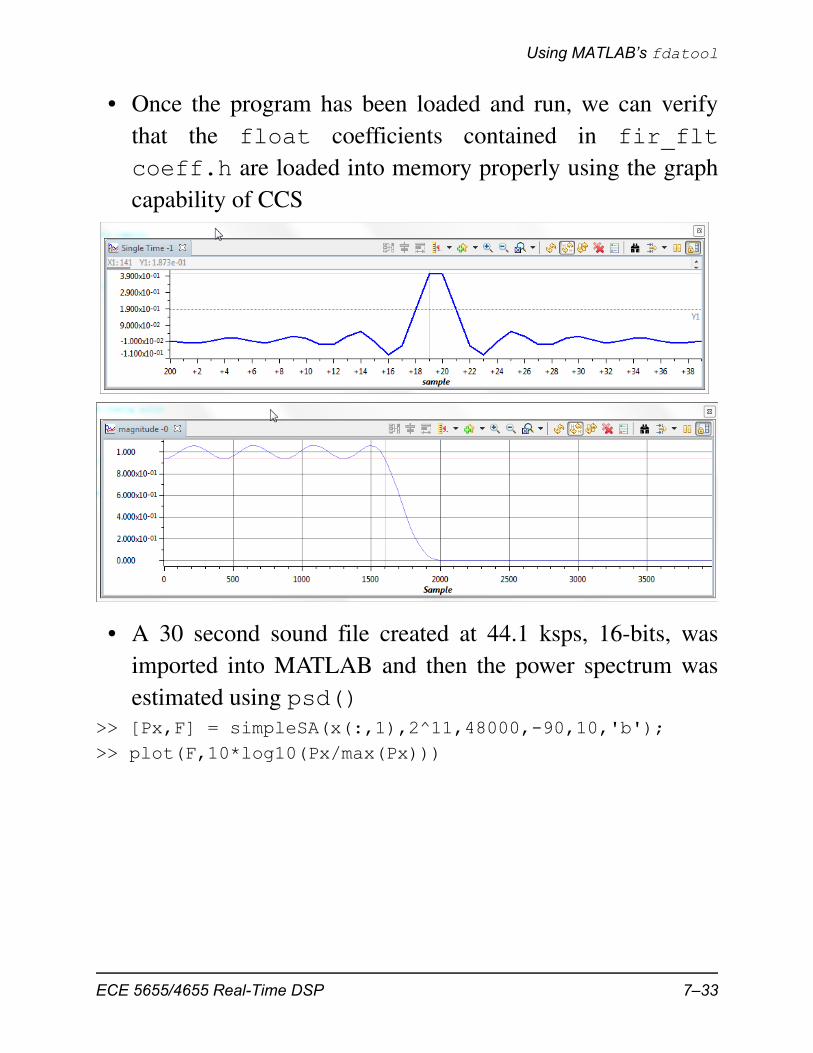
• Once the program has been loaded and run, we can verifythat the float coefficients contained in fir_fltcoeff.h are loaded into memory properly using the graphcapability of CCS
• A 30 second sound file created at 44.1 ksps, 16-bits, wasimported into MATLAB and then the power spectrum wasestimated using psd()
>> [Px,F] = simpleSA(x(:,1),2^11,48000,-90,10,'b');>> plot(F,10*log10(Px/max(Px)))
ECE 5655/4655 Real-Time DSP 7–33

Chapter 7 • Real-Time FIR Digital Filters
ISR Timing Results
• We see that the ISR running the 40 tap FIR requires a total of9 s
• In the limit this says when sampling at 8 ksps a maximum oftaps can be implemented
0 1000 2000 3000 4000 5000 6000 7000 8000−80
−70
−60
−50
−40
−30
−20
−10
0
Frequency (Hz)
Low
pass
Nor
mal
ized
Gai
n
fs 8 kHz=
fp 1.6 kHz=fs 2 kHz=
~60 dB
1 dB
Noise Test of Equiripple Linear-Phase FIR: N=40 (Order 39)(float coefficients)
125 40 9 555
7–34 ECE 5655/4655 Real-Time DSP
Using MATLAB’s fdatool
Code Enhancements
• The use of C intrinsics would allow us to utilize parallel mul-tiply accumulate operations
– This idea applies to word (32-bit) operations for the fixedfilter and double word operations on the C67 for the floatcase
• We have not yet used a circular buffer, which is part of theC6x special hardware capabilities
A Simple Fixed-Point Implementation
• Simple modification to the previous float FIR example yieldsa version using short integers
// Welch, Wright, & Morrow,
// Real‐time Digital Signal Processing, 2011
// Modified by Mark Wickert February 2012 to include GPIO ISR start/stop postings
///////////////////////////////////////////////////////////////////////
// Filename: ISRs_fir_short.c
//
// Synopsis: Interrupt service routine for codec data transmit/receive
// fixed point FIR filtering with coefficients in *.h file
//
///////////////////////////////////////////////////////////////////////
#include "DSP_Config.h"
#include "fir_fixcoeff.h" //coefficients in decimal format
// Function Prototypes
long int rand_int(void);
// Data is received as 2 16‐bit words (left/right) packed into one
// 32‐bit word. The union allows the data to be accessed as a single
// entity when transferring to and from the serial port, but still be
// able to manipulate the left and right channels independently.
#define LEFT 0
#define RIGHT 1
ECE 5655/4655 Real-Time DSP 7–35

Chapter 7 • Real-Time FIR Digital Filters
volatile union {
Uint32 UINT;
Int16 Channel[2];
} CodecDataIn, CodecDataOut;
/* add any global variables here */
short x_buffer[N_FIR]; //buffer for delay samples
interrupt void Codec_ISR()
///////////////////////////////////////////////////////////////////////
// Purpose: Codec interface interrupt service routine
//
// Input: None
//
// Returns: Nothing
//
// Calls: CheckForOverrun, ReadCodecData, WriteCodecData
//
// Notes: None
///////////////////////////////////////////////////////////////////////
{
/* add any local variables here */
WriteDigitalOutputs(1); // Write to GPIO J15, pin 6; begin ISR timing pulse
int i;
int result = 0; //initialize the accumulator
if(CheckForOverrun())// overrun error occurred (i.e. halted DSP)
return; // so serial port is reset to recover
CodecDataIn.UINT = ReadCodecData();// get input data samples
/* add your code starting here */
//Work with Left ADC sample
//x_buffer[0] = 0.25 * CodecDataIn.Channel[ LEFT];
//Use the next line to noise test the filter
x_buffer[0] = ((short) rand_int())>>3;//scale input by 1/8
//Filtering using a 32‐bit accumulator
for(i=0; i< N_FIR; i++)
{
result += x_buffer[i] * h[i];
}
//Update filter history
for(i=N_FIR‐1; i>0; i‐‐)
7–36 ECE 5655/4655 Real-Time DSP
Using MATLAB’s fdatool
{
x_buffer[i] = x_buffer[i‐1];
}
//Return 16‐bit sample to DAC; recall result is a 32 bit accumulator
CodecDataOut.Channel[ LEFT] = (short) (result >> 15);
// Copy Right input directly to Right output with no filtering
CodecDataOut.Channel[RIGHT] = CodecDataIn.Channel[ RIGHT];
/* end your code here */
WriteCodecData(CodecDataOut.UINT);// send output data to port
WriteDigitalOutputs(0); // Write to GPIO J15, pin 6; end ISR timing pulse
}
//White noise generator for filter noise testing
long int rand_int(void)
{
static long int a = 100001;
a = (a*125) % 2796203;
return a;
}
Writing fixed C Coefficient Files>> filter_C_header(Hd,'fixed','fir_fixcoeff.h',8)//define the FIR filter length
#define N_FIR 40
/*******************************************************************/
/* Filter Coefficients */
short h[N_FIR] = { ‐141, ‐429, ‐541, ‐211, 322, 354, ‐215, ‐551,
21, 736, 333, ‐841, ‐870, 755, 1651, ‐304,
‐2881,‐1107, 6139,13157,13157, 6139,‐1107,‐2881,
‐304, 1651, 755, ‐870, ‐841, 333, 736, 21,
‐551, ‐215, 354, 322, ‐211, ‐541, ‐429, ‐141 };
/*******************************************************************/
• The filter was tested with the OMAP-L138 board’s AIC3106and a white noise input generated in software
x_buffer[0] = ((short) rand_int())>>3;//scale input by 1/8
• A 30 second sound file created at 44.1 ksps, 16-bits, wasimported into MATLAB and then the power spectrum was
ECE 5655/4655 Real-Time DSP 7–37
Chapter 7 • Real-Time FIR Digital Filters
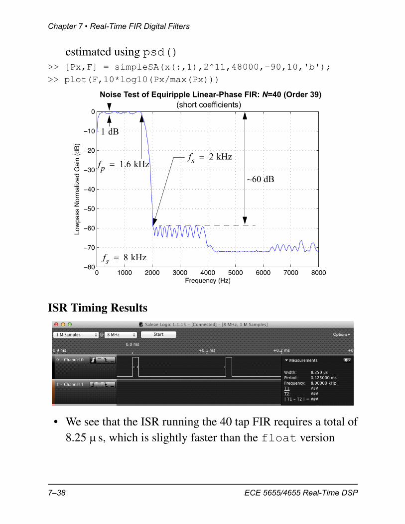
estimated using psd()>> [Px,F] = simpleSA(x(:,1),2^11,48000,-90,10,'b');>> plot(F,10*log10(Px/max(Px)))
ISR Timing Results
• We see that the ISR running the 40 tap FIR requires a total of8.25 s, which is slightly faster than the float version
0 1000 2000 3000 4000 5000 6000 7000 8000−80
−70
−60
−50
−40
−30
−20
−10
0
Frequency (Hz)
Low
pass
Nor
mal
ized
Gai
n (d
B)
fs 8 kHz=
fp 1.6 kHz=fs 2 kHz=
~60 dB
1 dB
Noise Test of Equiripple Linear-Phase FIR: N=40 (Order 39)(short coefficients)
7–38 ECE 5655/4655 Real-Time DSP
Circular Addressing
Circular Addressing
Circular Buffer in C
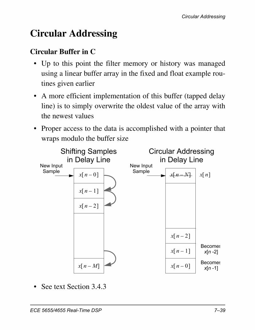
• Up to this point the filter memory or history was managedusing a linear buffer array in the fixed and float example rou-tines given earlier
• A more efficient implementation of this buffer (tapped delayline) is to simply overwrite the oldest value of the array withthe newest values
• Proper access to the data is accomplished with a pointer thatwraps modulo the buffer size
• See text Section 3.4.3
x n 0–
x n 1–
x n 2–
x n M–
Shifting Samplesin Delay Line
x n N–
x n 2–
x n 1–
x n 0–
New InputSample
New InputSample
Circular Addressingin Delay Line
x n
Becomesx[n -1]
Becomesx[n -2]
ECE 5655/4655 Real-Time DSP 7–39
Chapter 7 • Real-Time FIR Digital Filters
• See also TI Application Report SPRA645–June 2002
C Circular Buffer
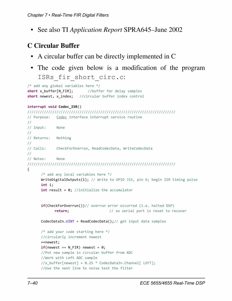
• A circular buffer can be directly implemented in C
• The code given below is a modification of the programISRs_fir_short_circ.c:
/* add any global variables here */
short x_buffer[N_FIR]; //buffer for delay samples
short newest, x_index; //circular buffer index control
interrupt void Codec_ISR()
///////////////////////////////////////////////////////////////////////
// Purpose: Codec interface interrupt service routine
//
// Input: None
//
// Returns: Nothing
//
// Calls: CheckForOverrun, ReadCodecData, WriteCodecData
//
// Notes: None
///////////////////////////////////////////////////////////////////////
{
/* add any local variables here */
WriteDigitalOutputs(1); // Write to GPIO J15, pin 6; begin ISR timing pulse
int i;
int result = 0; //initialize the accumulator
if(CheckForOverrun())// overrun error occurred (i.e. halted DSP)
return; // so serial port is reset to recover
CodecDataIn.UINT = ReadCodecData();// get input data samples
/* add your code starting here */
//circularly increment newest
++newest;
if(newest == N_FIR) newest = 0;
//Put new sample in circular buffer from ADC
//Work with Left ADC sample
//x_buffer[newest] = 0.25 * CodecDataIn.Channel[ LEFT];
//Use the next line to noise test the filter
7–40 ECE 5655/4655 Real-Time DSP
Circular Addressing
x_buffer[newest] = ((short) rand_int())>>3;//scale input by 1/8
//Filtering using a 32‐bit accumulator
x_index = newest;
for(i=0; i< N_FIR; i++)
{
result += h[i]*x_buffer[x_index];
//circularly decrement x_index
‐‐x_index;
if(x_index == ‐1) x_index = N_FIR‐1;
}
//Return 16‐bit sample to DAC; recall result is a 32 bit accumulator
CodecDataOut.Channel[ LEFT] = (short) (result >> 15);
// Copy Right input directly to Right output with no filtering
CodecDataOut.Channel[RIGHT] = CodecDataIn.Channel[ RIGHT];
/* end your code here */
WriteCodecData(CodecDataOut.UINT);// send output data to port
WriteDigitalOutputs(0); // Write to GPIO J15, pin 6; end ISR timing pulse
}
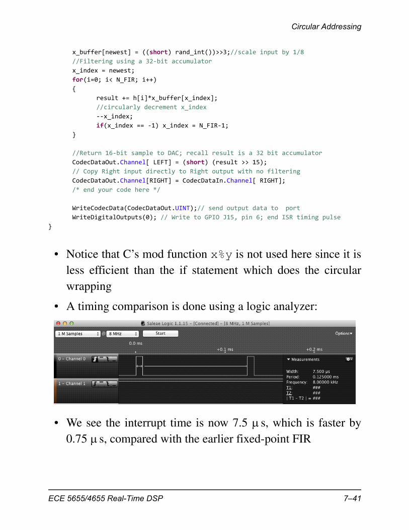
• Notice that C’s mod function x%y is not used here since it isless efficient than the if statement which does the circularwrapping
• A timing comparison is done using a logic analyzer:
• We see the interrupt time is now 7.5 s, which is faster by0.75 s, compared with the earlier fixed-point FIR
ECE 5655/4655 Real-Time DSP 7–41
Chapter 7 • Real-Time FIR Digital Filters
Circular Buffering via C Calling Assembly
• The C6x has underlying hardware to handle circular buffersetup and manipulation
• In the Chassaing text the programs FIRcirc.c, and whenusing external memory for the filter coefficients,FIRcirc_ext.c, take advantage of the C6x circularaddressing mode
– Details on the use of hardware circular addressing can befound in Chassaing Example 4.14 and Appendix B
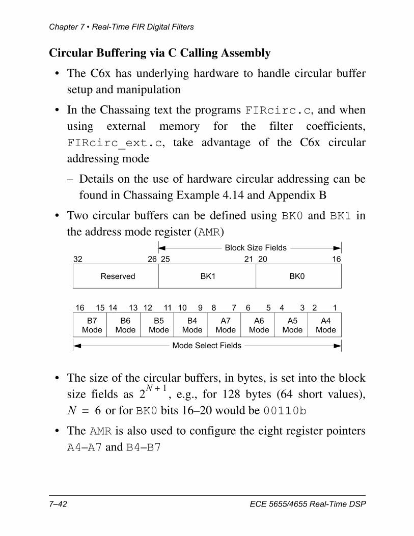
• Two circular buffers can be defined using BK0 and BK1 inthe address mode register (AMR)
• The size of the circular buffers, in bytes, is set into the blocksize fields as , e.g., for 128 bytes (64 short values),
or for BK0 bits 16–20 would be 00110b
• The AMR is also used to configure the eight register pointersA4–A7 and B4–B7
BK1 BK0
B7Mode
B6Mode
B5Mode
B4Mode
A7Mode
A6Mode
A5Mode
A4Mode
Reserved
162021252632
12345678910111213141516
Mode Select Fields
Block Size Fields
2N 1+
N 6=
7–42 ECE 5655/4655 Real-Time DSP
Circular Addressing
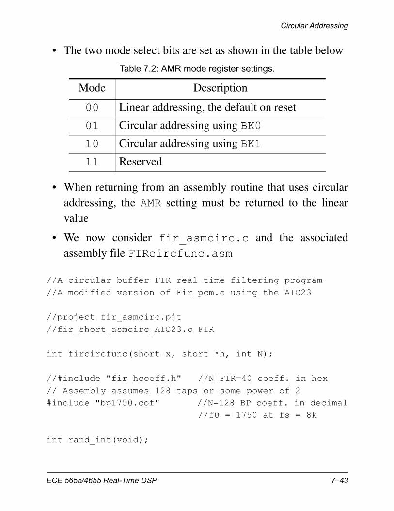
• The two mode select bits are set as shown in the table below
• When returning from an assembly routine that uses circularaddressing, the AMR setting must be returned to the linearvalue
• We now consider fir_asmcirc.c and the associatedassembly file FIRcircfunc.asm
//A circular buffer FIR real-time filtering program//A modified version of Fir_pcm.c using the AIC23
//project fir_asmcirc.pjt//fir_short_asmcirc_AIC23.c FIR
int fircircfunc(short x, short *h, int N);
//#include "fir_hcoeff.h" //N_FIR=40 coeff. in hex// Assembly assumes 128 taps or some power of 2#include "bp1750.cof" //N=128 BP coeff. in decimal //f0 = 1750 at fs = 8k
int rand_int(void);
Table 7.2: AMR mode register settings.
Mode Description
00 Linear addressing, the default on reset
01 Circular addressing using BK0
10 Circular addressing using BK1
11 Reserved
ECE 5655/4655 Real-Time DSP 7–43
Chapter 7 • Real-Time FIR Digital Filters
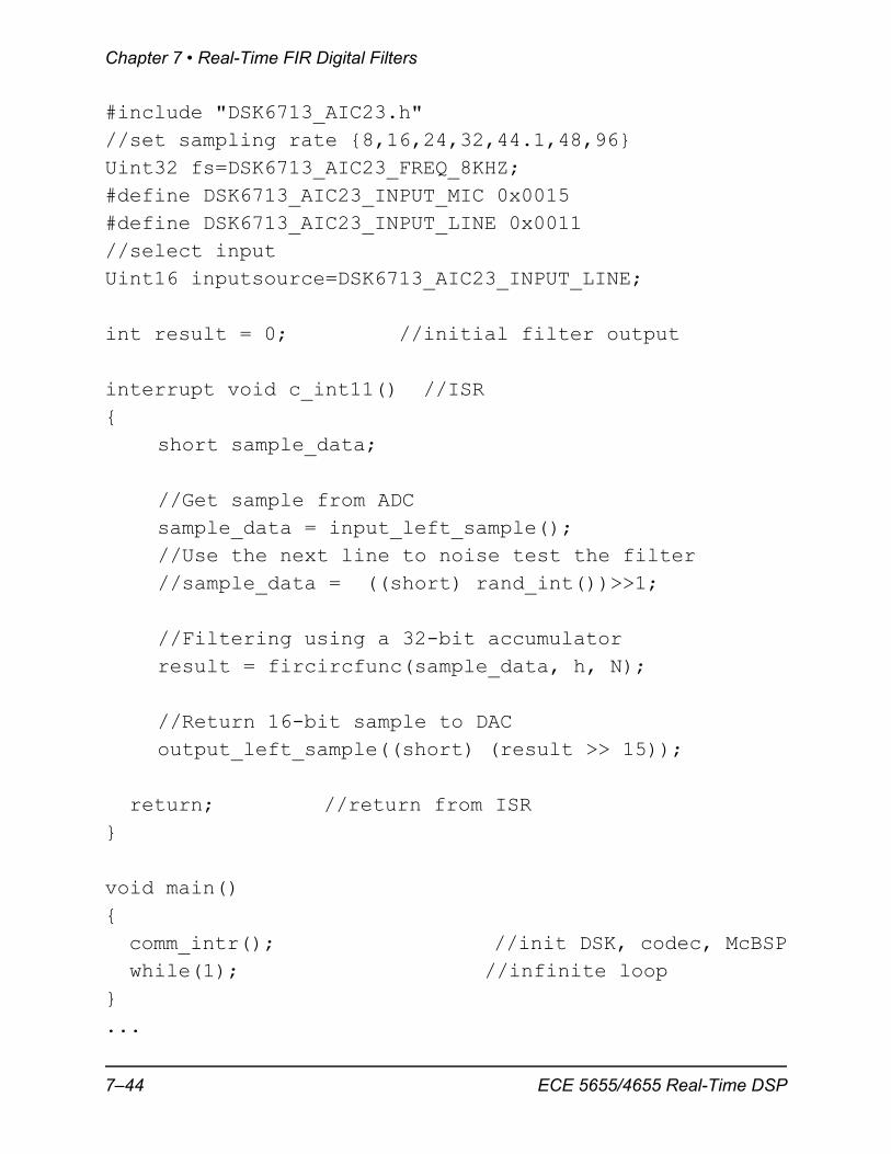
#include "DSK6713_AIC23.h"//set sampling rate {8,16,24,32,44.1,48,96}Uint32 fs=DSK6713_AIC23_FREQ_8KHZ;#define DSK6713_AIC23_INPUT_MIC 0x0015#define DSK6713_AIC23_INPUT_LINE 0x0011//select inputUint16 inputsource=DSK6713_AIC23_INPUT_LINE;
int result = 0; //initial filter output
interrupt void c_int11() //ISR{
short sample_data;
//Get sample from ADCsample_data = input_left_sample();//Use the next line to noise test the filter//sample_data = ((short) rand_int())>>1;
//Filtering using a 32-bit accumulatorresult = fircircfunc(sample_data, h, N);
//Return 16-bit sample to DACoutput_left_sample((short) (result >> 15));
return; //return from ISR}
void main(){ comm_intr(); //init DSK, codec, McBSP while(1); //infinite loop}...
7–44 ECE 5655/4655 Real-Time DSP
Circular Addressing
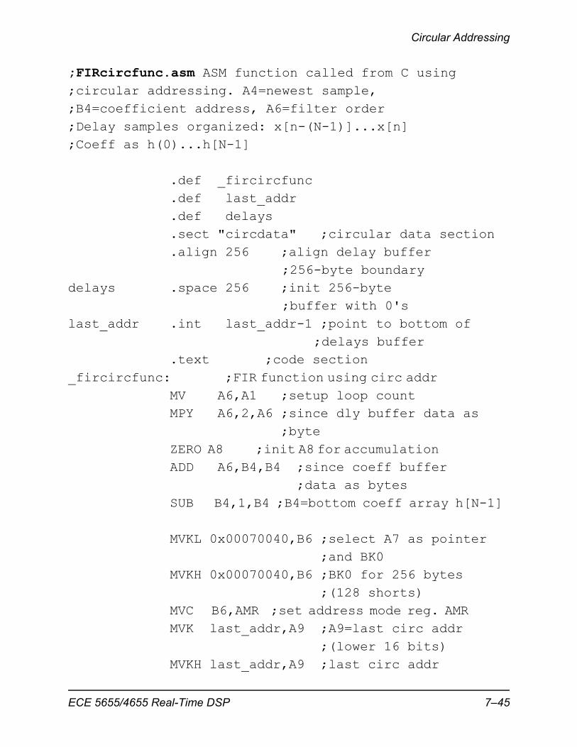
;FIRcircfunc.asm ASM function called from C using ;circular addressing. A4=newest sample, ;B4=coefficient address, A6=filter order ;Delay samples organized: x[n-(N-1)]...x[n];Coeff as h(0)...h[N-1]
.def _fircircfunc
.def last_addr
.def delays
.sect "circdata" ;circular data section
.align 256 ;align delay buffer ;256-byte boundarydelays .space 256 ;init 256-byte ;buffer with 0'slast_addr .int last_addr-1 ;point to bottom of ;delays buffer
.text ;code section_fircircfunc: ;FIR function using circ addr
MV A6,A1 ;setup loop count MPY A6,2,A6 ;since dly buffer data as ;byteZERO A8 ;init A8 for accumulation ADD A6,B4,B4 ;since coeff buffer ;data as bytesSUB B4,1,B4 ;B4=bottom coeff array h[N-1]
MVKL 0x00070040,B6 ;select A7 as pointer ;and BK0MVKH 0x00070040,B6 ;BK0 for 256 bytes ;(128 shorts) MVC B6,AMR ;set address mode reg. AMR MVK last_addr,A9 ;A9=last circ addr ;(lower 16 bits)MVKH last_addr,A9 ;last circ addr
ECE 5655/4655 Real-Time DSP 7–45
Chapter 7 • Real-Time FIR Digital Filters
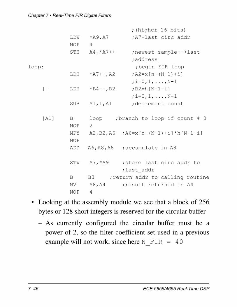
;(higher 16 bits) LDW *A9,A7 ;A7=last circ addrNOP 4 STH A4,*A7++ ;newest sample-->last ;address
loop: ;begin FIR loopLDH *A7++,A2 ;A2=x[n-(N-1)+i] ;i=0,1,...,N-1
|| LDH *B4--,B2 ;B2=h[N-1-i] ;i=0,1,...,N-1SUB A1,1,A1 ;decrement count
[A1] B loop ;branch to loop if count # 0NOP 2MPY A2,B2,A6 ;A6=x[n-(N-1)+i]*h[N-1+i]NOP ADD A6,A8,A8 ;accumulate in A8
STW A7,*A9 ;store last circ addr to ;last_addrB B3 ;return addr to calling routineMV A8,A4 ;result returned in A4NOP 4
• Looking at the assembly module we see that a block of 256bytes or 128 short integers is reserved for the circular buffer
– As currently configured the circular buffer must be apower of 2, so the filter coefficient set used in a previousexample will not work, since here N_FIR = 40
7–46 ECE 5655/4655 Real-Time DSP
Circular Addressing
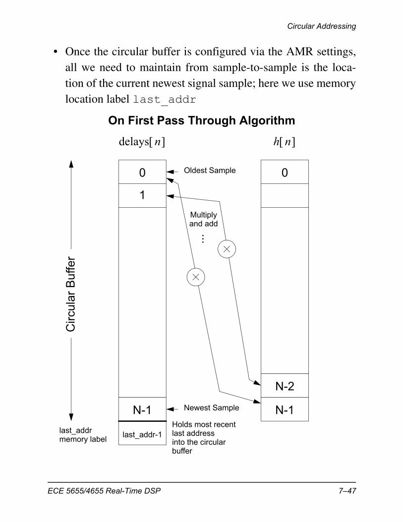
• Once the circular buffer is configured via the AMR settings,all we need to maintain from sample-to-sample is the loca-tion of the current newest signal sample; here we use memorylocation label last_addr
h n delays n
0
N-1 N-1
N-2
0
last_addr-1
Newest Sample
Oldest Sample
Circ
ular
Buf
fer
last_addrmemory label
Holds most recentlast addressinto the circularbuffer
...1
On First Pass Through Algorithm
Multiplyand add
ECE 5655/4655 Real-Time DSP 7–47
Chapter 7 • Real-Time FIR Digital Filters
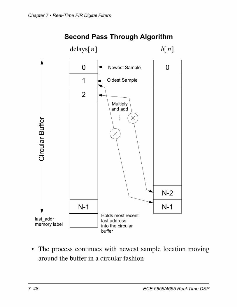
• The process continues with newest sample location movingaround the buffer in a circular fashion
h n delays n
0
N-1 N-1
N-2
0
Oldest Sample
Newest Sample
Circ
ular
Buf
fer
last_addrmemory label
Holds most recentlast addressinto the circularbuffer
...
1
Second Pass Through Algorithm
Multiplyand add
2
7–48 ECE 5655/4655 Real-Time DSP

Performance of Interrupt Driven Programs
Performance of Interrupt Driven Programs
• In the development of real-time signal processing systems,there are clearly performance trade-offs to be made
• The character of all the interrupt driven programs we haveseen thus far is that:
– We first load system parameters into memory, e.g., filtercoefficients
– Next registers are initialized on the CPU and serial port isconfigured
– The appropriate interrupt is enabled on the CPU
– The program then enters an infinite (wait) loop
– While in this infinite loop the CPU is interrupted at thesampling rate of samples per second by the AIC23,which has new analog I/O samples to exchange
– Before returning to the wait loop again, the program exe-cutes code that carries out the desired signal processingtasks (Note: here we assume for simplicity that there areno other background signal processing tasks to be per-formed)
• In order for the DSP application to maintain true real-timestatus, all signal processing computations must be completedbefore the next codec initiated interrupt is fired
• Debugging interrupt driven programs is not a simple matter
fs
ECE 5655/4655 Real-Time DSP 7–49
Chapter 7 • Real-Time FIR Digital Filters
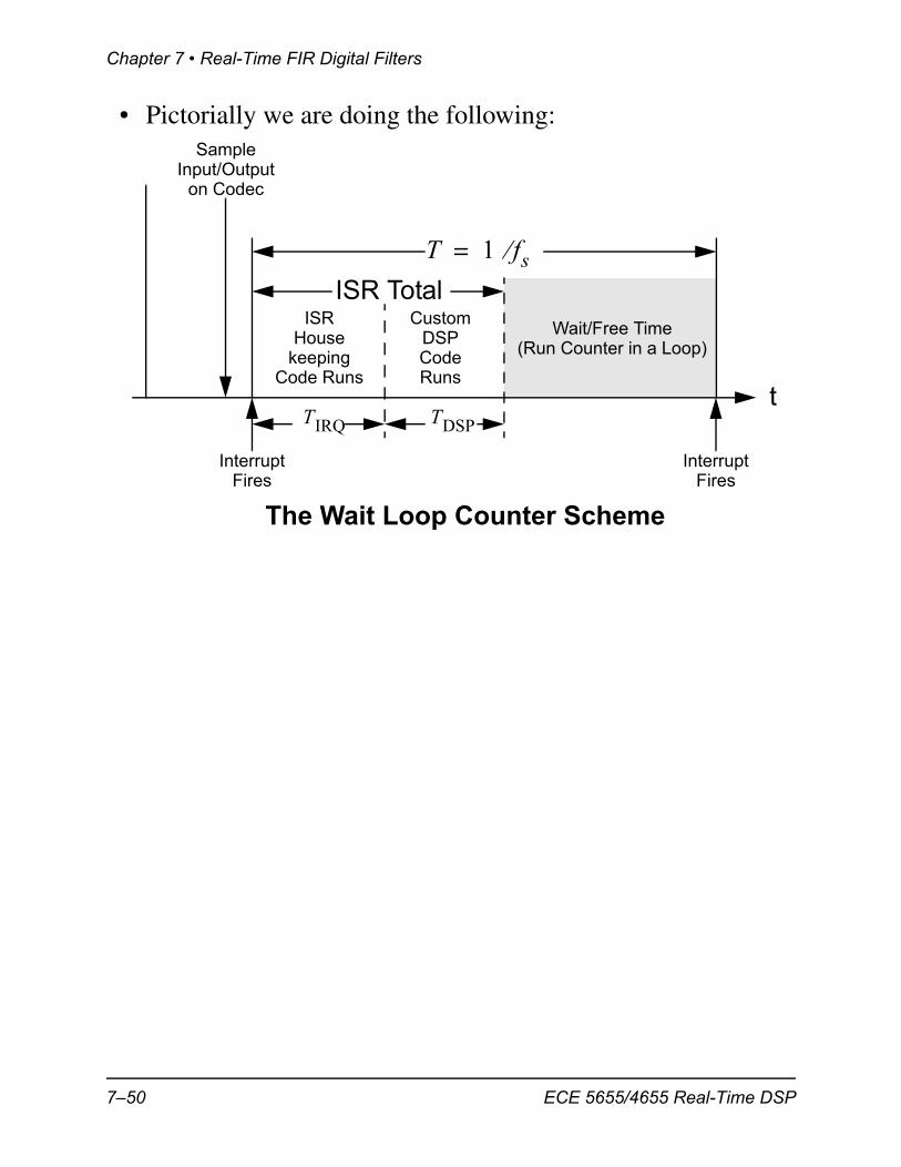
• Pictorially we are doing the following:
InterruptFires
ISRHouse
keepingCode Runs
CustomDSPCodeRuns
SampleInput/Output
on Codec
t
InterruptFires
T 1 fs=
ISR TotalWait/Free Time
(Run Counter in a Loop)
The Wait Loop Counter Scheme
TIRQ TDSP
7–50 ECE 5655/4655 Real-Time DSP
C5515 Code Example
C5515 Code Example
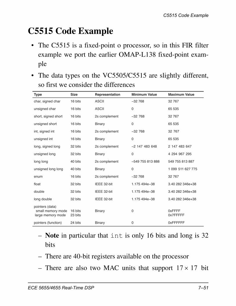
• The C5515 is a fixed-point o processor, so in this FIR filterexample we port the earlier OMAP-L138 fixed-point exam-ple
• The data types on the VC5505/C5515 are slightly different,so first we consider the differences
– Note in particular that int is only 16 bits and long is 32bits
– There are 40-bit registers available on the processor
– There are also two MAC units that support bit
Type Size Representation Minimum Value Maximum Value
char, signed char 16 bits ASCII −32 768 32 767
unsigned char 16 bits ASCII 0 65 535
short, signed short 16 bits 2s complement −32 768 32 767
unsigned short 16 bits Binary 0 65 535
int, signed int 16 bits 2s complement −32 768 32 767
unsigned int 16 bits Binary 0 65 535
long, signed long 32 bits 2s complement −2 147 483 648 2 147 483 647
unsigned long 32 bits Binary 0 4 294 967 295
long long 40 bits 2s complement −549 755 813 888 549 755 813 887
unsigned long long 40 bits Binary 0 1 099 511 627 775
enum 16 bits 2s complement −32 768 32 767
float 32 bits IEEE 32-bit 1.175 494e−38 3.40 282 346e+38
double 32 bits IEEE 32-bit 1.175 494e−38 3.40 282 346e+38
long double 32 bits IEEE 32-bit 1.175 494e−38 3.40 282 346e+38
pointers (data) small memory mode large memory mode
16 bits 23 bits
Binary 0 0xFFFF0x7FFFFF
pointers (function) 24 bits Binary 0 0xFFFFFF
17 17
ECE 5655/4655 Real-Time DSP 7–51
Chapter 7 • Real-Time FIR Digital Filters
multiplies
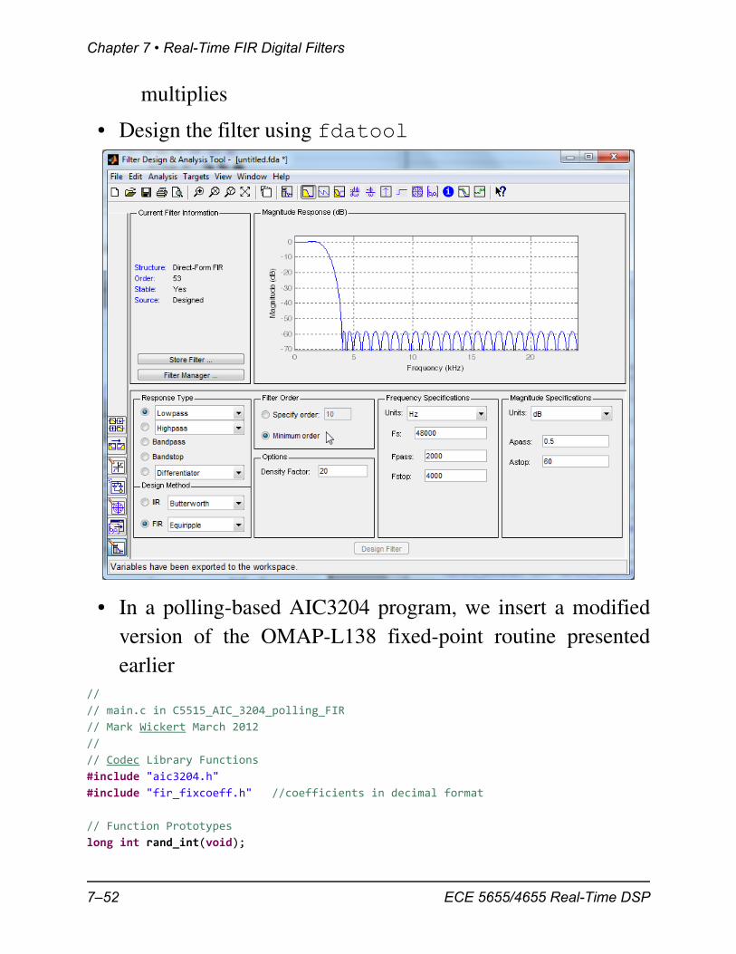
• Design the filter using fdatool
• In a polling-based AIC3204 program, we insert a modifiedversion of the OMAP-L138 fixed-point routine presentedearlier
//
// main.c in C5515_AIC_3204_polling_FIR
// Mark Wickert March 2012
//
// Codec Library Functions
#include "aic3204.h"
#include "fir_fixcoeff.h" //coefficients in decimal format
// Function Prototypes
long int rand_int(void);
7–52 ECE 5655/4655 Real-Time DSP
C5515 Code Example
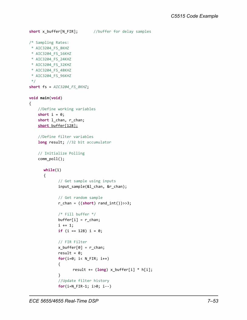
short x_buffer[N_FIR]; //buffer for delay samples
/* Sampling Rates:
* AIC3204_FS_8KHZ
* AIC3204_FS_16KHZ
* AIC3204_FS_24KHZ
* AIC3204_FS_32KHZ
* AIC3204_FS_48KHZ
* AIC3204_FS_96KHZ
*/
short fs = AIC3204_FS_8KHZ;
void main(void)
{
//Define working variables
short i = 0;
short l_chan, r_chan;
short buffer[128];
//Define filter variables
long result; //32 bit accumulator
// Initialize Polling
comm_poll();
while(1)
{
// Get sample using inputs
input_sample(&l_chan, &r_chan);
// Get random sample
r_chan = ((short) rand_int())>>3;
/* Fill buffer */
buffer[i] = r_chan;
i += 1;
if (i == 128) i = 0;
// FIR Filter
x_buffer[0] = r_chan;
result = 0;
for(i=0; i< N_FIR; i++)
{
result += (long) x_buffer[i] * h[i];
}
//Update filter history
for(i=N_FIR‐1; i>0; i‐‐)
ECE 5655/4655 Real-Time DSP 7–53

Chapter 7 • Real-Time FIR Digital Filters
{
x_buffer[i] = x_buffer[i‐1];
}
/* Write Digital audio input */
output_sample(l_chan, (short)(result>>16));
//output_sample(l_chan, r_chan);
}
}
//White noise generator for filter noise testing
long int rand_int(void)
{
static long int a = 100001;
a = (a*125) % 2796203;
return a;}
// fir_fixcoeff.h
//define the FIR filter length
#define N_FIR 40
/*******************************************************************/
/* Filter Coefficients */
short h[N_FIR] = { ‐141, ‐429, ‐541, ‐211, 322, 354, ‐215, ‐551,
21, 736, 333, ‐841, ‐870, 755, 1651, ‐304,
‐2881,‐1107, 6139,13157,13157, 6139,‐1107,‐2881,
‐304, 1651, 755, ‐870, ‐841, 333, 736, 21,
‐551, ‐215, 354, 322, ‐211, ‐541, ‐429, ‐141 };
/*******************************************************************/
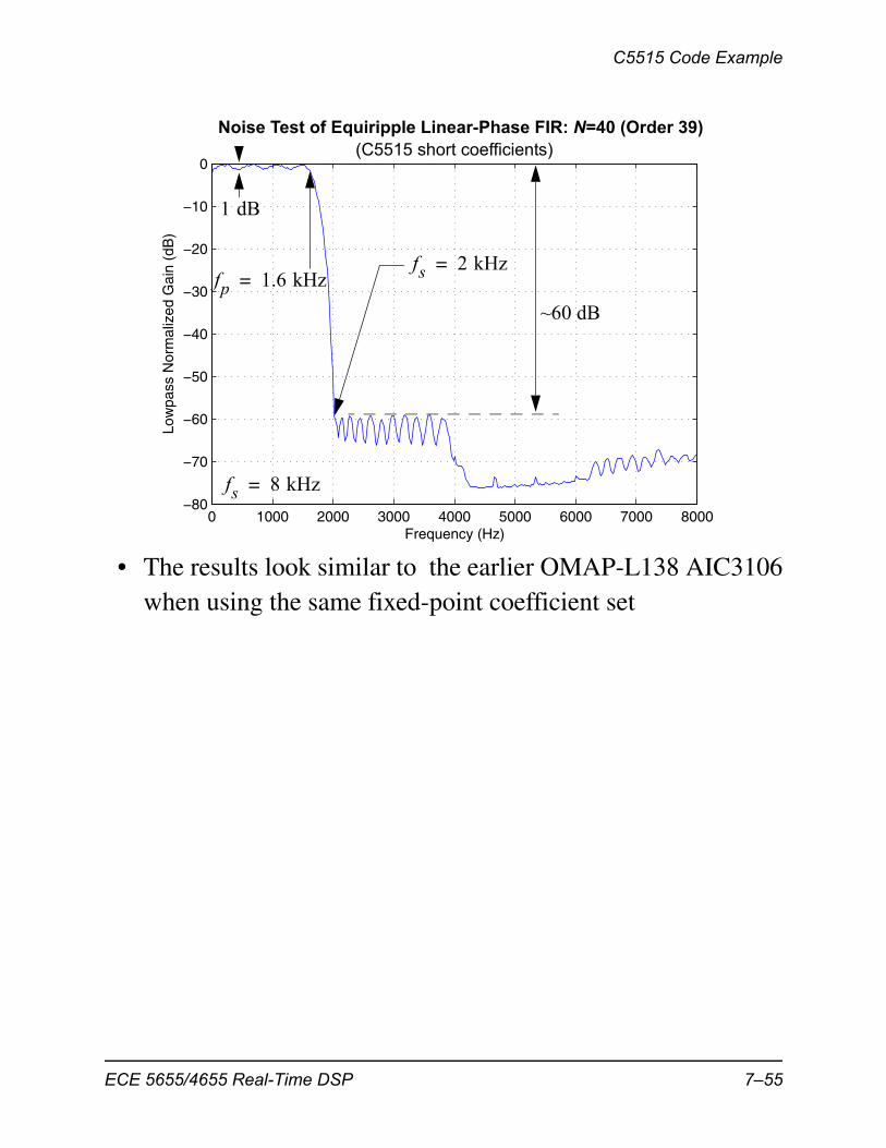
• Audio noise capture of a 2 kHz lowpass filter, assuming asampling rate of 48 kHz
>> [Px,F] = simpleSA(x(:,2),2^11,48000,-90,10,'b');>> plot(F,10*log10(Px/max(Px)))>> axis([0 8000 -80 0])
7–54 ECE 5655/4655 Real-Time DSP
C5515 Code Example
• The results look similar to the earlier OMAP-L138 AIC3106when using the same fixed-point coefficient set
0 1000 2000 3000 4000 5000 6000 7000 8000−80
−70
−60
−50
−40
−30
−20
−10
0
Frequency (Hz)
Low
pass
Nor
mal
ized
Gai
n (d
B)
fs 8 kHz=
fp 1.6 kHz=fs 2 kHz=
~60 dB
1 dB
Noise Test of Equiripple Linear-Phase FIR: N=40 (Order 39)(C5515 short coefficients)
ECE 5655/4655 Real-Time DSP 7–55
Chapter 7 • Real-Time FIR Digital Filters
7–56 ECE 5655/4655 Real-Time DSP
Related Documents