Real-Time Data Warehousing with Oracle Business ... · BI/Data Warehousing/EPM 2 257 Figure 2: Real-time Data Warehousing Options. STAGING LAYER The Staging layer is the “landing

REAL-TIME DATA WAREHOUSING WITH ORACLE BUSINESS

INTELLIGENCE AND ORACLE DATABASE

Stewart Bryson, Rittman Mead

INTRODUCTION

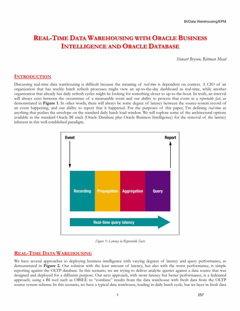
Discussing real-time data warehousing is difficult because the meaning of real-time is dependent on context. A CIO of an organization that has weekly batch refresh processes might view an up-to-the-day dashboard as real-time, while another organization that already has daily refresh cycles might be looking for something closer to up-to-the-hour. In truth, an interval will always exist between the occurrence of a measurable event and our ability to process that event as a reportable fact, as demonstrated in Figure 1. In other words, there will always be some degree of latency between the source-system record of an event happening, and our ability to report that it happened. For the purposes of this paper, I’m defining real-time as anything that pushes the envelope on the standard daily batch load window. We will explore some of the architectural options available in the standard Oracle BI stack (Oracle Database plus Oracle Business Intelligence) for the removal of the latency inherent in this well-established paradigm.

REAL-TIME DATA WAREHOUSING

We have several approaches to deploying business intelligence with varying degrees of latency and query performance, as demonstrated in Figure 2. Our solution with the least amount of latency, but also with the worst performance, is simple reporting against the OLTP database. In this scenario, we are trying to deliver analytic queries against a data source that was designed and deployed for a different purpose. Our next approach, with more latency but better performance, is a federated approach, using a BI tool such as OBIEE to “combine” results from the data warehouse with fresh data from the OLTP source system schema. In this scenario, we have a typical data warehouse, loading in daily batch cycle, but we layer in fresh data

BI/Data Warehousing/EPM

1 257

!"##$%!&'"()!"#"$%&'(##%)*+)%'(,-*./")%0*1"%#(%2"%)3$"%(4%#0"%.""5%2"4($"%#0"+%/.)/)#%(.%$"*67#/,"%23)/."))/.#"66/8".'"9

!"#$%&#'()*#&)%+,-./)#$(/01-.23#4(&#%-#+)%*-#5#6(0)#-6)#)23.2)#/%2%3)/)2-7#-&%$-.(2#$(2-&(+#%2'#89:#*"*-)/*#%&)#&)%+#-./);<=

!"#/(>.+)#06(2)#.*#&)%+#-./)7#)?)2#*(/)#(@#/"#6(/)#)2-)&-%.2/)2-#3%'3)-*#%&)#&)%+#-./)#A#>1-#B6%-#%>(1-#>1*.2)**

.2-)++.3)2$)#*"*-)/*C

52#-6)#)%&+"#'%"*#(@#95#4(&#B%*#.-#$%++)'#')$.*.(2#*100(&-#>%$D#-6)2C<#&)0(&-.23#'%-%#@(&#-6)#$1&&)2-#/(2-6#B%*#%2#%$6.)?)/)2-=

8*#-)$62.E1)*#%2'#-)$62(+(3.)*#)?(+?)'7#$(/0%2.)*#/(?)'#-(#&)0(&-#(2#-6)#0&)?.(1*#'%"#>1-#B)&)#*-.++#&)+.%2-#(2#%2#(1-,(@,

6(1&*#>%-$6#0&($)**#-(#/(?)#'%-%#@&(/#-6)#*(1&$)#*"*-)/*#%2'#*-(&)#%2'#%33&)3%-)#.-#.2#-6).&#'%-%#B%&)6(1*)*#%2'#'%-%

/%&-*=

91-#B.-6#FG,6(1&#>1*.2)**#'%"*#%2'#-6)#2))'#-(#&)0(&-#%$&(**#/1+-.0+)#-./),H(2)*7#-6)#-&%'.-.(2%+#>%-$6#B.2'(B#.*#>).23

*E1))H)'#.2-(#2)%&#2(2,)I.*-)2$)=#J)B#'%-%#)I-&%$-.(2#%2'#+(%'#0%&%'.3/*#6%?)#%+*(#>))2#')?)+(0)'#-(#-&.$D+),@))'#&)0(&-.23

*"*-)/*=#91-#%&)#-6)*)#&)%++"#&)%+#-./)#A#%2'#'()*#.-#&)%++"#/%--)&C

52#&)%+.-"7#-6)&)#.*#%+B%"*#3(.23#-(#>)#%#')3&))#(@#+%-)2$"#>)-B))2#%2#)?)2-#6%00)2.23#%2'#.-#>).23#&)$(&')'#(2#%#-&%2*%$-.(2%+

*"*-)/7#0&(0%3%-)'#-(#-6)#&)0(&-.23#*"*-)/7#+(%')'7#%2'#@.2%++"#%33&)3%-)'#(2#%#'%-%#B%&)6(1*)#>)@(&)#>).23#&)%'"#-(#E1)&"=

8''#-(#-6%-#-6)#')+%"#>)-B))2#-6)#1*)&#.**1.23#%#E1)&"#-6%-#%$$)**)*#-6.*#2)B#2133)-#(@#.2@(&/%-.(2#%2'#-6)#&)*1+-#>).23

&)-1&2)'#-(#-6)#1*)&7#%2'#"(1#@.2'#%#'.*$)&2.>+)#+%3#>)-B))2#)?)2-#%2'#(>*)&?%-.(2=

K&1)7#-6)&)#%&)#-6.23*#"(1#$%2#'(#-(#/.-.3%-)#-6.*#+%3#>1-#-6)&)#B.++#%+B%"*#>)#%#$(10+)#(@#*-)0*#.2#-6)#0&($)**#B6)&)#&)'1$.23

(2)#-./)#0)&.('#.2$&)%*)*#%2(-6)&#A#@(&#)I%/0+)7#"(1#$%2#*6(&-)2#&)0(&-#)I)$1-.(2#-./)#>"#%33&)3%-.23#-6)#'%-%#-(#>)--)&

%2*B)&#-6)#E1)&"7#>1-#-6.*#*-)0#%''*#/(&)#-./)#-(#-6)#'%-%#+(%'#%2'#%33&)3%-)#06%*)=

L1&-6)&/(&)7#'.@@)&)2-#-"0)*#(@#.2$(/.23#'%-%#$%2#6%?)#'.@@)&.23#+%-)2$.)*=#L(&#)I%/0+)7#%#2)B#-&%2*%$-.(2#/%"#6%?)#%#*6(&-)&

+%-)2$"#-6%2#%#$6%23)#-(#%#&)3.(2%+#3&(10.23#(@#*-(&)*#-6%-#/%"#2))'#-(#>)#0&(0%3%-)'#-6&(136#/%2"#+%")&*#(@#6.*-(&.$%+

%33&)3%-.(2#-%>+)*#4*))#L.31&)#M<=

K6)#'.?.*.(2#>)-B))2#'%-%#%$E1.*.-.(2#%2'#'%-%#0&)*)2-%-.(2#0&)*)2-*#%#D)"#E1)*-.(2#-6%-#%2"#$(/0%2"#2))'*#-(#%2*B)&#B6)2

$(2-)/0+%-.23#/(?.23#-(#%#&)%+,-./)#95#*"*-)/N#%&)#"(1#O1*-#.2-)&)*-)'#.2#0&(?.'.237#%*#&%0.'+"#%*#0(**.>+)7#.2@(&/%-.(2#>%*)'

(2#%+&)%'"#%$E1.&)'#'%-%7#(&#'(#"(1#%+*(#2))'#-(#&)0(&-#(2#2)B+"#%'')'#@%$-1%+#.2@(&/%-.(2C

L(&#)I%/0+)7#%#B(&D)&#.2#%#/(>.+)#06(2)#$(/0%2"P*#$%++

$)2-&)#/%"#+.D)#-(#*))#.2@(&/%-.(2#%>(1-#Q6(B#3(('#%

$1*-(/)&#.*P#%2'#-6)#+.D)+.6(('#-6%-#*(/)(2)#B.-6.2#-6%-

$1*-(/)&P*#')/(3&%06.$#B(1+'#*B.-$6#-(#%2(-6)&#

*100+.)&=

K6.*#.2@(&/%-.(2#2))'*#-(#>)#0&)*)2-)'#E1.$D+"#4B6.+*-#-6)"

%&)#*0)%D.23#-(#-6)/<#%2'#0&)@)&%>+"#B.-6.2#-6)#$(2-)I-#(@#-6)

+.2),(@,>1*.2)**#%00+.$%-.(2#-6%-#/%2%3)*#-6)#$1*-(/)&

.2-)&%$-.(2=#R(B)?)&#.-#.*#12+.D)+"#-6%-#%2"#(@#-6)#/)-&.$*#1*)'

>"#-6)#$%++#$)2-&)#%3)2-#@(&#$1*-(/)&#0&(@.-%>.+.-"#%2'

0&)'.$-)'#$61&2#B(1+'#>)#.2@+1)2$)'#>"#)?)2-*#(@#-6)#+%*-#@)B

6(1&*=

S(2?)&*)+"7#%#*"*-)/#-6%-#.*#1*.23#)/>)'')'#95#@12$-.(2%+.-"

-(#%+)&-#-(#0(-)2-.%+#@&%1'#4*-($D#/%&D)-*#%2'#$&)'.-#$%&'

$(/0%2.)*#%&)#0(**.>+)#)I%/0+)#1*)&*<#/%"#B)++#2))'#-(

D2(B#%>(1-#10,-(,-6),/(/)2-#%$-.?.-"=

***+,-./0.12345,416,+537

FIGURE 1: BI latency

Recording Propagation Aggregation Query

Event Report

Real-time query latency

Figure 1: Latency in Reportable Facts

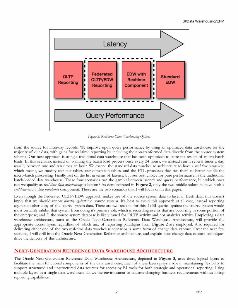
from the source for intra-day records. We improve upon query performance by using an optimized data warehouse for the majority of our data, with gains for real-time reporting by including the non-tranformed data directly from the source system schema. Our next approach is using a traditional data warehouse that has been optimized to store the results of micro-batch loads. In this scenario, instead of running the batch load process once every 24 hours, we instead run it several times a day, usually between one and ten times an hour. We extend the standard data warehouse architecture to have a real-time component, which means, we modify our fact tables, our dimension tables, and the ETL processes that run them to better handle the micro-batch processing. Finally, last on the list in terms of latency, but our best choice for pure performance, is the traditional, batch-loaded data warehouse. These four scenarios run the gambit between latency and query performance, but which ones can we qualify as real-time data warehousing solutions? As demonstrated in Figure 2, only the two middle solutions have both a real-time and a data warehouse component. These are the two scenarios that I will focus on in this paper.

Even though the Federated OLTP/EDW approach makes use of the source system data to layer in fresh data, this doesn’t imply that we should report directly against the source system. It’s best to avoid this approach at all cost, instead reporting against another copy of the source system data. There are two reasons for this: 1) BI queries against the source system would most certainly inhibit that system from doing it’s primary job, which is recording events that are occurring in some portion of the enterprise; and 2) the source system database is likely tuned for OLTP activity and not analytics activity. Employing a data warehouse architecture, such as the Oracle Next-Generation Reference Data Warehouse Architecture, will provide the appropriate access layers regardless of which mix of reporting paradigms from Figure 2 are employed. Also required for delivering either one of the two real-time data warehouse scenarios is some form of change data capture. Over the next few sections, I will drill into the Oracle Next-Generation Reference architecture, and explain how change-data capture techniques drive the delivery of this architecture.

NEXT-GENERATION REFERENCE DATA WAREHOUSE ARCHITECTURE

The Oracle Next-Generation Reference Data Warehouse Architecture, depicted in Figure 3, uses three logical layers to facilitate the main functional components of the data warehouse. Each of these layers plays a role in maintaining flexibility to support structured and unstructured data sources for access by BI tools for both strategic and operational reporting. Using multiple layers in a single data warehouse allows the environment to address changing business requirements without losing reporting capabilities.

BI/Data Warehousing/EPM

2 257

Figure 2: Real-time Data Warehousing Options

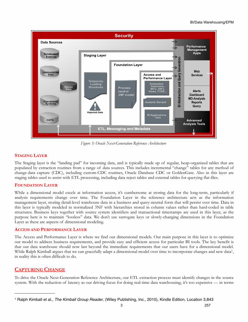
STAGING LAYER

The Staging layer is the “landing pad” for incoming data, and is typically made up of regular, heap-organized tables that are populated by extraction routines from a range of data sources. This includes incremental “change” tables for any method of change-data capture (CDC), including custom-CDC routines, Oracle Database CDC or GoldenGate. Also in this layer are staging tables used to assist with ETL processing, including data reject tables and external tables for querying flat-files.

FOUNDATION LAYER

While a dimensional model excels at information access, it’s cumbersome at storing data for the long-term, particularly if analysis requirements change over time. The Foundation Layer in the reference architecture acts as the information management layer, storing detail-level warehouse data in a business and query-neutral form that will persist over time. Data in this layer is typically modeled in normalized 3NF with hierarchies stored in column values rather than hard-coded in table structures. Business keys together with source system identifiers and transactional timestamps are used in this layer, as the purpose here is to maintain “lossless” data. We don’t use surrogate keys or slowly-changing dimensions in the Foundation Layer as these are aspects of dimensional modeling.

ACCESS AND PERFORMANCE LAYER

The Access and Performance Layer is where we find our dimensional models. Our main purpose in this layer is to optimize our model to address business requirements, and provide easy and efficient access for particular BI tools. The key benefit is that our data warehouse should now last beyond the immediate requirements that our users have for a dimensional model. While Ralph Kimball argues that we can gracefully adapt a dimensional model over time to incorporate changes and new data1, in reality this is often difficult to do.

CAPTURING CHANGE

To drive the Oracle Next-Generation Reference Architecture, our ETL extraction process must identify changes in the source system. With the reduction of latency as our driving focus for doing real-time data warehousing, it’s too expensive — in terms

BI/Data Warehousing/EPM

3 257

1 Ralph Kimball et al., The Kimball Group Reader, (Wiley Publishing, Inc., 2010), Kindle Edition, Location 3,843

Figure 3: Oracle Next-Generation Reference Architecture

of time and processing against the source system — for us to drive a real-time data warehousing approach without a change-data capture system. Oracle provides the following two solutions for standard change-data capture:

• Oracle Change Data Capture (CDC)• Oracle GoldenGate

Both of these options are superior to hand-coded SQL for determining changes, or manual detection systems that use triggers, because they use the REDO already generated by the system for fault tolerance. GoldenGate is the technologically superior choice: it’s simple, flexible, powerful and resilient. It does, however, fall outside the standard Oracle BI stacks, so for the purposes of this paper, we will consider Oracle CDC only. Oracle CDC is included with Oracle Database Enterprise Edition, and employs different combinations of LogMiner, Streams and Advanced Queues depending on the flavor selected, as demonstrated in Figure 4 below. Streams will continue to be the “free” option for data replication, and will always provide the technical implementation of the Oracle CDC feature of the database. However, GoldenGate is the preferred replication technology moving forward, so we shouldn’t expect to see many feature enhancements to Streams or CDC. Regardless of the technology selected, generic change tables would exist in the Staging layer of the data warehouse architecture.

FEDERATED OLTP/EDW REPORTING

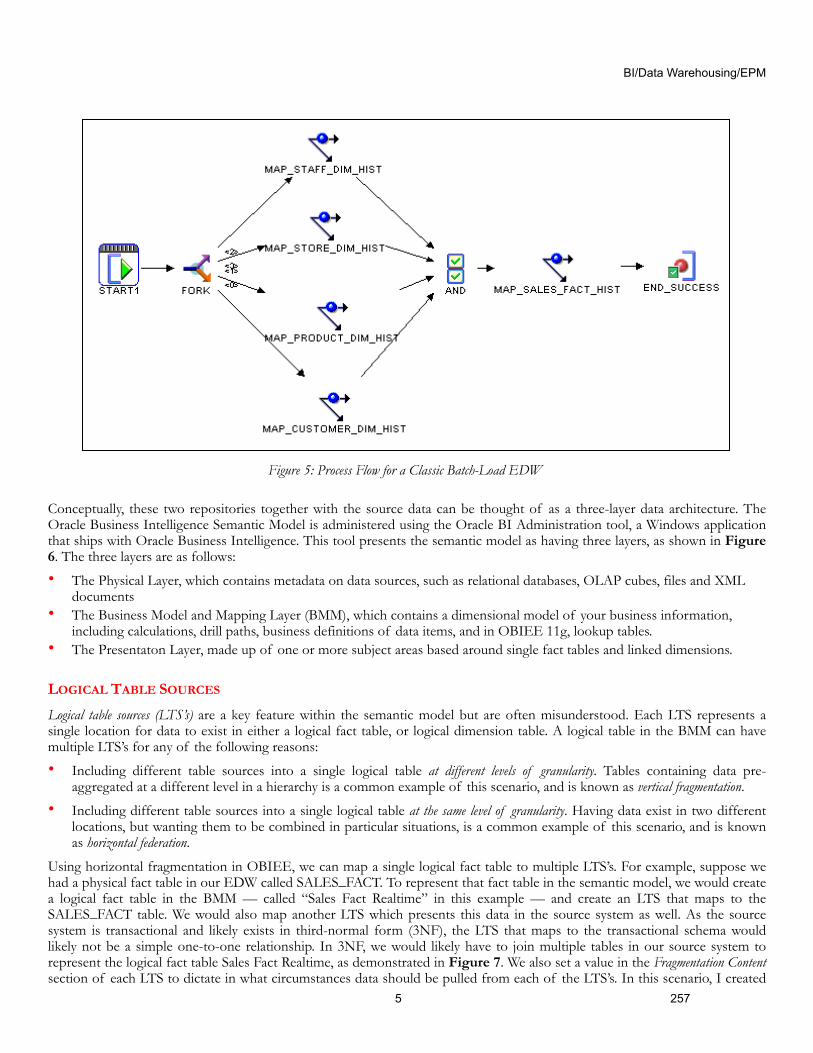
The typical approach in Federated OLTP/EDW reporting environments is to use a BI tool such as OBIEE to do horizontal federation: which means combining data from multiple sources at the same grain in a single table. One of the sources for federation is a classic, batch-loaded EDW, with ETL processes that load conformed dimension tables, followed by fact tables that store the measures and calculations for the enterprise. Oracle Warehouse Builder (OWB), the ETL tool built inside the Oracle Database, is a standard choice for data warehouses built on the Oracle Database. In Figure 5, we can see a simplified process flow for how a small subject area in an EDW might be loaded. To understand how OBIEE can combine data from an EDW with data from a source system schema, we first need to understand the OBIEE Semantic Model.

THE OBIEE SEMANTIC MODEL

Oracle Business Intelligence, like a number of enterprise business intelligence tool, has a metadata layer that aims to hide the complexity of underlying data sources and present information using business terminology. This metadata layer is called the Semantic Model and is stored in a repository, held in a single file usually referred to as an RPD file, after the file extension that it uses. The repository is accessed and navigated by a process in OBIEE called the BI Server. This metadata layer works alongside a separate repository used for holding reports, dashboards and other presentation objects, called the Web Catalog.

BI/Data Warehousing/EPM

4 257

Figure 4: Different Oracle Asynchronous CDC Implementations

Conceptually, these two repositories together with the source data can be thought of as a three-layer data architecture. The Oracle Business Intelligence Semantic Model is administered using the Oracle BI Administration tool, a Windows application that ships with Oracle Business Intelligence. This tool presents the semantic model as having three layers, as shown in Figure 6. The three layers are as follows:

• The Physical Layer, which contains metadata on data sources, such as relational databases, OLAP cubes, files and XML documents

• The Business Model and Mapping Layer (BMM), which contains a dimensional model of your business information, including calculations, drill paths, business definitions of data items, and in OBIEE 11g, lookup tables.

• The Presentaton Layer, made up of one or more subject areas based around single fact tables and linked dimensions.

LOGICAL TABLE SOURCES

Logical table sources (LTS’s) are a key feature within the semantic model but are often misunderstood. Each LTS represents a single location for data to exist in either a logical fact table, or logical dimension table. A logical table in the BMM can have multiple LTS’s for any of the following reasons:

• Including different table sources into a single logical table at different levels of granularity. Tables containing data pre-aggregated at a different level in a hierarchy is a common example of this scenario, and is known as vertical fragmentation.

• Including different table sources into a single logical table at the same level of granularity. Having data exist in two different locations, but wanting them to be combined in particular situations, is a common example of this scenario, and is known as horizontal federation.

Using horizontal fragmentation in OBIEE, we can map a single logical fact table to multiple LTS’s. For example, suppose we had a physical fact table in our EDW called SALES_FACT. To represent that fact table in the semantic model, we would create a logical fact table in the BMM — called “Sales Fact Realtime” in this example — and create an LTS that maps to the SALES_FACT table. We would also map another LTS which presents this data in the source system as well. As the source system is transactional and likely exists in third-normal form (3NF), the LTS that maps to the transactional schema would likely not be a simple one-to-one relationship. In 3NF, we would likely have to join multiple tables in our source system to represent the logical fact table Sales Fact Realtime, as demonstrated in Figure 7. We also set a value in the Fragmentation Content section of each LTS to dictate in what circumstances data should be pulled from each of the LTS’s. In this scenario, I created

BI/Data Warehousing/EPM

5 257

Figure 5: Process Flow for a Classic Batch-Load EDW

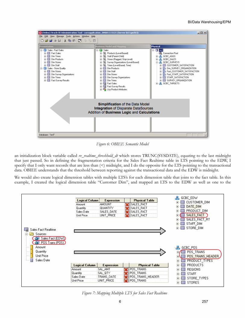
an initialization block variable called rv_realtime_threshhold_dt which stores TRUNC(SYSDATE), equating to the last midnight that just passed. So in defining the fragmentation criteria for the Sales Fact Realtime table in LTS pointing to the EDW, I specify that I only want records that are less than (<) midnight, and I do the opposite for the LTS pointing to the transactional data. OBIEE understands that the threshold between reporting against the transactional data and the EDW is midnight.

We would also create logical dimension tables with multiple LTS’s for each dimension table that joins to the fact table. In this example, I created the logical dimension table “Customer Dim”, and mapped an LTS to the EDW as well as one to the

BI/Data Warehousing/EPM

6 257

Figure 6: OBIEE Semantic Model

Figure 7: Mapping Multiple LTS for Sales Fact Realtime

transaction data, as shown in Figure 8. The interesting part about these LTS’s is that they won’t require a fragmentation threshold to be configured because we rely on the fragmentation threshold configured for Sales Fact Realtime to adequately segment the two sources.

LOGICAL UNION

What’s the result of all this complex mapping among different LTS’s in the BMM? OBIEE understands that each source schema is completely segmented, and the tables in each LTS never join to tables in the other LTS… but they do union. OBIEE will construct a complete query against the transactional schema, in this example, joining between the

CUSTOMER_DEMOG_TYPES, CUSTOMERS, POS_TRANS and POS_TRANS_HEADER tables. Additionally, OBIEE will construct another complete query against the EDW schema, in this case, only the tables SALES_FACT and CUSTOMER_DIM. OBIEE then logically unions the results between the two source schemas into a single result set that is returned whenever a user builds a report against the logical tables Customer Dim and Sales Fact Realtime.

What’s most interesting is how OBIEE does the logical union. When the EDW and the transactional schema exist in separate databases, the BI Server issues two different queries and combines them into a single result set in it’s own memory space. However, if the different schemas exist within the same database, as the Oracle Next-Generation Reference Architecture recommends, then the BI Server is able to issue a single query, transforming the logical union into an actual physical union in the SQL statement, as demonstrated in the statement below. Notice that the SQL threshold has been applied, and the UNION was constructed with a single SQL statement pushed down from the BI Server to the Oracle Database holding the Foundation and Presentation and Access layers in our Oracle architecture:

WITH SAWITH0 AS ((select T43901.CUST_FIRST_NAME as c2, T43901.CUST_LAST_NAME as c3, T43971.SAL_AMT as c4from GCBC_CRM.CUSTOMERS T43901, GCBC_POS.POS_TRANS T43971, GCBC_POS.POS_TRANS_HEADER T43978

BI/Data Warehousing/EPM

7 257

Figure 8: Mapping Multiple LTS for Customer Dim

where ( T43901.CUST_ID = T43978.CUST_ID and T43971.TRANS_ID = T43978.TRANS_ID and TO_DATE('2010-09-18 00:00:00' , 'YYYY-MM-DD HH24:MI:SS') < T43978.TRANS_DATE ) union allselect T44042.CUSTOMER_FIRST_NAME as c2, T44042.CUSTOMER_LAST_NAME as c3, T44105.AMOUNT as c4from GCBC_EDW.CUSTOMER_DIM T44042, GCBC_EDW.SALES_FACT T44105where ( T44042.CUSTOMER_KEY = T44105.CUSTOMER_KEY ) )),SAWITH1 AS (select sum(D3.c4) as c1, D3.c2 as c2, D3.c3 as c3from SAWITH0 D3group by D3.c2, D3.c3)select distinct 0 as c1, D2.c2 as c2, D2.c3 as c3, D2.c1 as c4from SAWITH1 D2

EDW WITH A REAL-TIME COMPONENT

Whereas the Federated OLTP/EDW Reporting option provides us an option to layer real-time data into an otherwise classic batch-loaded EDW, delivering the EDW with a Real-Time Component requires designing an EDW from the ground up that supports real-time reporting. Specifically, we have to design our fact tables to support what Ralph Kimball calls the “real-time partition”. “To achieve real-time reporting, we build a special partition that is physically and administratively separated from the conventional static data warehouse tables. Actually, the name partition is a little misleading. The real-time partition may be a separate table, subject to special rules for update and query.”2 So we construct a separate section for each of our fact tables to facilitate the following four requirements, as defined by Kimball:3

• Contain all activity since the last time the load was run• Link seamlessly to the grain of the static data warehouse tables• Be indexed so lightly that incoming data can “dribble in”• Support highly responsive queries

In Figure 9, we see how the real-time partition is structurally identical to the static data warehouse table, but it is a completely separate structure.

ETL

So we modify our model to support the interaction of real-time and static data, but we also modify our ETL to support this. In fact, to construct an EDW with a Real-Time Component, we have to build some very intricate interaction between the database, the data model and ETL processes. The static fact table is partitioned on a date data-type using standard Oracle partitioning strategies. The real-time partition is structured in such a way as to be able to load throughout the day. In other words, there are no indexes or constraints enabled on the table. ETL is typically loaded into real-time partition using a process comparable to a traditional load scenario, but operated instead using micro-batch, running as much as 100 times a day, or even more. Alternative methods include transactional style, record-by-record loading, possible using web services or message-based system such as JMS queues.

BI/Data Warehousing/EPM

8 257

2 Kimball, Location 13,227

3 Kimball, Location 13,231

EARLY-ARRIVING FACTS

We have one issue with the load of the real-time partition: we are assuming that we receive all of our dimension data right along with our fact data in clean CDC subscription groups. That would likely be the case if we were pulling all the records for our data warehouse from a single source-system, but with enterprise data warehouses, that is rarely the case. Receiving dimension data early causes no problems with our load scenario; it doesn’t matter if we do the surrogate key lookup for the fact table load hours or days later than the dimensions. Receiving the fact table data early does present us with ETL logic issues: the correct dimension record may or may not be there when it’s time to load the facts.

There is a simple strategy to handle early-arriving facts. In our ETL, we move through the process to below to ensure that our facts are at least reportable intra-day:

1. If a dimension record exists for the current business or natural key we are interested in, then grab the latest. This is the best we can do, and quite often, it will be the correct value.

2. If no dimension record exists yet for the current natural key, then use a default record type equating to “Not Known Yet.” Though it’s not sexy for intra-day reporting, it at least makes the data available across the dimensions we do know about. We can see what this mapping will look like in Figure 10. An outer-join to the early-arriving dimension — in this case the CUSTOMER_DIM table — provides the information necessary to attach the “Not Known Yet” record.

3. As we approach the end of the day and prepare to “close the books” for the current day, we should have run all dimension loads so that our dimension tables are all up to date.

4. We run a corrective mapping to update all the fact records in the real-time partition with the right surrogate keys.

PARTITIONING

When “closing the books” on the day, we build indexes and constraints on the real-time partition that match those on the partitioned fact table. Once this step is complete, we can then use a partition-exchange operation to combine the real-time partition as part of the static fact table. In Oracle, this is a fast, dictionary update, and occurs almost instantaneously.

Obviously, our partitioning choice for the fact table will determine exactly how this partition-exchange will occur. If we’ll agree to partition the fact table by DAY, then we can use Oracle Interval partitioning, available in Oracle 11gR1 and beyond. We have to make this concession because Interval partitioning tables cannot have partitions in the same table that contain different range-based boundaries. For instance, we can’t have some MONTH-based partitions, while also having some DAY-based partitions. Using Interval partitioning is the easiest method, however, because it requires the least amount of partition maintenance as part of the load. For instance, consider the SALES_FACT table listed below, using Interval partitioning on the SALES_DATE_KEY, which we partition on at the DAY grain:

BI/Data Warehousing/EPM

9 257

Figure 9: Separate but Equal Real-Time Partition

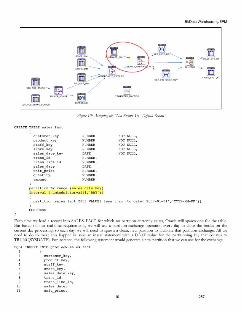
CREATE TABLE sales_fact ( customer_key NUMBER NOT NULL, product_key NUMBER NOT NULL, staff_key NUMBER NOT NULL, store_key NUMBER NOT NULL, sales_date_key DATE NOT NULL, trans_id NUMBER, trans_line_id NUMBER, sales_date DATE, unit_price NUMBER, quantity NUMBER, amount NUMBER ) partition BY range (sales_date_key) interval (numtodsinterval(1,'DAY')) ( partition sales_fact_2006 VALUES less than (to_date('2007-01-01','YYYY-MM-DD')) ) COMPRESS/

Each time we load a record into SALES_FACT for which no partition currently exists, Oracle will spawn one for the table. But based on our real-time requirements, we will use a partition-exchange operation every day to close the books on the current day processing, so each day, we will need to spawn a clean, new partition to facilitate that partition-exchange. All we need to do to make this happen is issue an insert statement with a DATE value for the partitioning key that equates to TRUNC(SYSDATE). For instance, the following statement would generate a new partition that we can use for the exchange:

SQL> INSERT INTO gcbc_edw.sales_fact 2 ( 3 customer_key, 4 product_key, 5 staff_key, 6 store_key, 7 sales_date_key, 8 trans_id, 9 trans_line_id, 10 sales_date, 11 unit_price,

BI/Data Warehousing/EPM

10 257

Figure 10: Assigning the “Not Known Yet” Default Record

12 quantity, 13 amount) 14 VALUES 15 ( 16 -1, 17 -1, 18 -1, 19 -1, 20 trunc(SYSDATE), 21 -1, 22 -1, 23 SYSDATE, 24 0, 25 0, 26 0 27 ) 28 /

1 row created.

Elapsed: 00:00:00.01SQL>

Once the insert has created our new SYSDATE-based partition, we can exchange the real-time partition in for this new partition. We can use the new PARTITION FOR clause — which allows us to reference partition names using partition key values — with a slight caveat. Though we can’t use SYSDATE explicitly in the DDL statement, we can reference it implicitly:

SQL> DECLARE 2 l_date DATE := SYSDATE; 3 l_sql LONG; 4 BEGIN 5 l_sql := q'|alter table gcbc_edw.sales_fact exchange partition|' 6 || chr(10) 7 || q'|for ('|' 8 || l_date 9 || q'|') with table gcbc_edw.sales_fact_rt|'; 10 11 dbms_output.put_line( l_sql ); 12 EXECUTE IMMEDIATE( l_sql ); 13 END; 14 /

alter table gcbc_edw.sales_fact exchange partitionfor ('03/01/2011 09:38:33 PM') with table gcbc_edw.sales_fact_rt

PL/SQL procedure successfully completed.

Elapsed: 00:00:00.07SQL>

If our requirements involve partitioning the fact table using higher-level periods, such as MONTH or QUARTER, then we will have to use standard RANGE-based partitioning, which will require partition-maintenance processes which will split a single “DAY” off of the current MAX partition so the real-time partition can then be exchanged in. Afterwards, a merge-partition process can be implemented to combine the two partitions again.

Using the preferred Interval partitioning option, the final “Close the Books” process flow is shown in Figure 11. The first step that is taken is to run any late-arriving dimension mappings, in this example, the MAP_CUSTOMER_DIM mapping. Once all the dimensions are up-to-date, we can run the process that corrects all the dimension keys in the real-time partition. Remember, the real-time partition contains small data sets, so updating these records should not be resource intensive. In this

BI/Data Warehousing/EPM

11 257

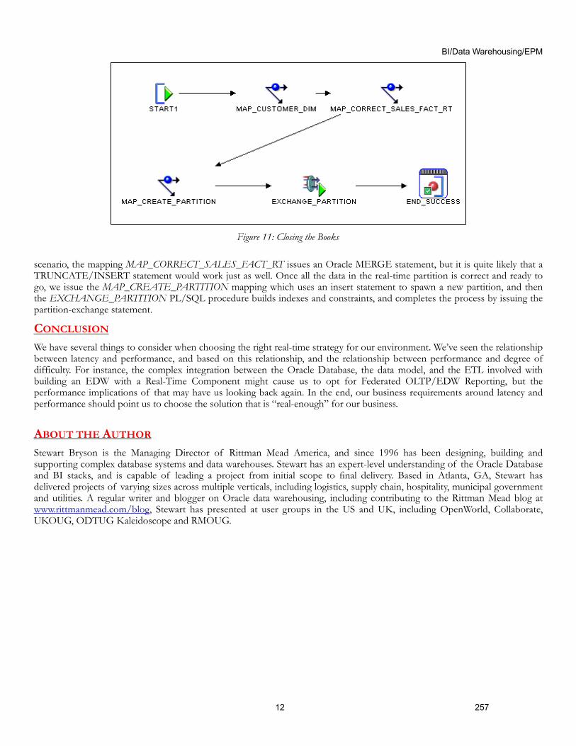
scenario, the mapping MAP_CORRECT_SALES_FACT_RT issues an Oracle MERGE statement, but it is quite likely that a TRUNCATE/INSERT statement would work just as well. Once all the data in the real-time partition is correct and ready to go, we issue the MAP_CREATE_PARTITION mapping which uses an insert statement to spawn a new partition, and then the EXCHANGE_PARTITION PL/SQL procedure builds indexes and constraints, and completes the process by issuing the partition-exchange statement.

CONCLUSION

We have several things to consider when choosing the right real-time strategy for our environment. We’ve seen the relationship between latency and performance, and based on this relationship, and the relationship between performance and degree of difficulty. For instance, the complex integration between the Oracle Database, the data model, and the ETL involved with building an EDW with a Real-Time Component might cause us to opt for Federated OLTP/EDW Reporting, but the performance implications of that may have us looking back again. In the end, our business requirements around latency and performance should point us to choose the solution that is “real-enough” for our business.

ABOUT THE AUTHOR

Stewart Bryson is the Managing Director of Rittman Mead America, and since 1996 has been designing, building and supporting complex database systems and data warehouses. Stewart has an expert-level understanding of the Oracle Database and BI stacks, and is capable of leading a project from initial scope to final delivery. Based in Atlanta, GA, Stewart has delivered projects of varying sizes across multiple verticals, including logistics, supply chain, hospitality, municipal government and utilities. A regular writer and blogger on Oracle data warehousing, including contributing to the Rittman Mead blog at www.rittmanmead.com/blog, Stewart has presented at user groups in the US and UK, including OpenWorld, Collaborate, UKOUG, ODTUG Kaleidoscope and RMOUG.

BI/Data Warehousing/EPM

12 257

Figure 11: Closing the Books