Submitted by Dipl.-Ing. Bernadett Stadler, BSc. Submitted at Industrial Mathematics Institute Supervisor and First Evaluator Univ.-Prof. Dr. Ronny Ramlau Second Evaluator Prof. Lothar Reichel Co-Supervisor Dr. Roberto Biasi October 2021 JOHANNES KEPLER UNIVERSITY LINZ Altenbergerstraße 69 4040 Linz, O sterreich www.jku.at DVR 0093696 Real-time computing methods for astronomical adaptive optics Doctoral Thesis to obtain the academic degree of Doktorin der technischen Wissenschaften in the Doctoral Program Technische Wissenschaften

Welcome message from author
This document is posted to help you gain knowledge. Please leave a comment to let me know what you think about it! Share it to your friends and learn new things together.
Transcript

Submitted byDipl.-Ing.Bernadett Stadler, BSc.
Submitted atIndustrial MathematicsInstitute
Supervisor andFirst EvaluatorUniv.-Prof. Dr.Ronny Ramlau
Second EvaluatorProf. Lothar Reichel
Co-SupervisorDr. Roberto Biasi
October 2021
JOHANNES KEPLERUNIVERSITY LINZAltenbergerstraße 694040 Linz, Osterreichwww.jku.atDVR 0093696
Real-time computingmethods for astronomicaladaptive optics
Doctoral Thesis
to obtain the academic degree of
Doktorin der technischen Wissenschaften
in the Doctoral Program
Technische Wissenschaften


Abstract
Astronomical imaging with ground-based telescopes suffers from quickly varying opticaldistortions, which cause blurring and loss of contrast. These optical distortions areinduced by turbulences in the earth’s atmosphere. Since the contrast and sharpness ofimages are essential for astronomical observations, a method that compensates for theseaberrations is required. This technique is called Adaptive Optics (AO). It utilizes acombination of wavefront sensors, that measure the deformations of wavefronts emittedby guide stars, and deformable mirrors to correct for them. Classical AO systems, usingonly one guide star, achieve high image quality only near to this guide star. Since thereare not enough bright guide stars available close to scientific objects of interest, AOsystems that achieve a good correction over a large field have been developed. Thesesystems involve a tomographic estimation of the 3D atmospheric wavefront disturbance.Mathematically, the reconstruction of turbulent layers in the atmosphere is severely ill-posed, hence, limits the achievable solution accuracy. Moreover, the reconstruction hasto be performed in real-time at a few hundred to thousand Hertz frame rates. This leadsto a computational challenge, especially for the AO systems of future Extremely LargeTelescopes (ELTs) with a primary mirror up to 40 m.
The aim of this work is to develop and implement an efficient real-time reconstructionalgorithm on the high-performance hardware of the industrial partner Microgate. Inparticular, we present a novel, conjugate gradient (CG) based method called augmentedFinite Element Wavelet Hybrid Algorithm (augmented FEWHA) for atmospheric to-mography. Our method is based on the classical FEWHA, which uses a dual-domaindiscretization strategy to obtain sparse operators. The matrix-free representation ofthese operators leads to a significant reduction in the computational load and mem-ory. Moreover, the method is highly parallelizable. A crucial indicator for the run-timeof iterative solvers is the number of iterations. We extend the classical FEWHA withan augmented Krylov subspace method in order to reduce the number of CG iterations.Moreover, we provide an efficient, parallel implementation of both algorithms on a multi-core CPU and a GPU. We analyze the performance of augmented FEWHA in terms ofquality and run-time via numerical simulations for ELT-sized test configurations. Asa quality benchmark we use the classical FEWHA, which is known to yield excellentresults. In terms of run-time augmented FEWHA requires less CG iterations comparedto the classical version, which results in a significant performance boost.
i


Zusammenfassung
Die astronomische Bilderfassung mit erdgebundenen Teleskopen leidet stark unter sichschnell veränderten optischen Effekten, welche Unschärfe und Kontrastverlust zur Folgehaben. Diese Störungen werden durch Turbulenzen in der Erdatmosphäre hervorgerufen.Um die Bildqualität zu verbessern, werden sogenannte Adaptive Optik (AO) Systemeeingesetzt. Diese Systeme benutzen Wellenfrontsensoren, welche die Aberrationen derLichtwellen von Leitsternen erkennen, sowie verformbare Spiegel, welche die atmosphäri-schen Störungen kompensieren. Klassische AO Syteme benutzen lediglich einen Leit-stern und erreichen deshalb einen hohe Bildqualität nur für Objekte in der Nähe diesesSterns. Da nicht genug helle Leitsterne für beliebige astronomische Objekte verfüg-bar sind, wurden AO Systeme entwickelt die eine gute Bildqualität über ein breitesSichtfeld liefern. Solche System erfordern die tomografische Berechnung der dreidi-mensionale atmospherischen Wellenfrontstörungen. Aus mathematischer Sicht ist dieseProblem schlecht gestellt, d.h. die Lösungsgenauigkeit ist stark eingeschränkt. Zudemmuss die Rekonstruktion in Echtzeit, bei einer Bildrate von einigen hunderten bis zutausend Hertz, passieren. Dies führt zur erheblichen Herausforderungen im Bereichder Rechenleistung, im Speziellen für die AO Syteme der zukünfigen Riesenteleskopen(ELTs), welche einen Primärspiegel von bis zu 40 m besitzen.
Das Ziel dieser Arbeit ist es, einen effiziente Echtzeitrekonstruktor zu entwickeln undin die Hardware des Industriepartners Microgate zu integrieren. Wir präsentieren denaugmented Finite Element Wavelet Hybrid Algorithm (augmented FEWHA), welcherauf dem klassichen FEWHA beruht und somit auf der Methode der konjugierten Gradi-enten. FEWHA benutzt eine duale Domän-Diskretisierungsstrategie, um eine effizientematrixfreie Darstellung aller zugrundeliegender Operatoren zu erhalten. Diese Darstel-lung reduziert den Rechenaufwand und die Speicherauslatung erheblich. Außerdem istder Algorithmus sehr gut parallelisierbar. Ein entscheidender Faktor für die Laufzeit it-erativer Löser ist die Anzahl der Iterationen. In dieser Arbeit erweitern wir FEWHA miteiner augmentierten Krylov-Unterraum-Methode und reduzieren so die Anzahl der Iter-ationen. Außerdem präsentieren wir eine parallele Implementierung beider Algorithmenauf einer multi-core CPU und einer GPU. Wir analysieren die Leistung des Algorithmushinsichtlich Qualität und Laufzeit für ELT Testkonfigurationen. Letzendlich ist es unsmöglich bei gleichbleibender Qualität die Anzahl der Iterationen für augmented FEWHAzu verringern und so die Laufzeit deutlich zu reduzieren.
iii


Acknowledgements
Foremost, I would like to express my deepest gratitude to my academic supervisor Prof.Ronny Ramlau and my industrial supervisor Dr. Roberto Biasi for giving me the uniqueopportunity to be involved in the enthralling work for the ELT. I totally appreciate theirsupport and guidance, but also the trust and freedom they offered to me.
It was an honor to have Prof. Lothar Reichel as a second referee. I am grateful for thetime he invested in reading this thesis, his support and the inspiration he gave me.
I would like to express my kindest thanks to my colleagues from the Austrian AdaptiveOptics team (Andreas Obereder, Stefan Raffetseder, Julia Shatokhina, Roland Wagner,Günter Auzinger, Simon Hubmer, Jenny Niebsch, Viktoria Hutterer, Martin Schwals-berger), especially, for sharing their expertise in the field of Adaptive Optics, whichthey built up over years. Moreover, my deep gratitude goes to my colleagues at Micro-gate (Mauro Manetti, Christian Patauner, Dietrich Pesacoller, Gerald Angerer, MarioAndrighettoni and Maurizio Groppi) for their frequent help and support, for fruitfuldiscussions, and cordial friendship. I also want to express my kindest thanks to mycolleagues in the European Industrial Doctorate program ROMSOC, especially, to theother Early Stage Researchers, who became close friends.
Without the constant support of my family, boyfriend and friends I would not be whereI am right now. I am truly thankful to my parents for encouraging me to follow mydreams and for offering me the trust and aid I needed to go my own way. The deepgratefulness I feel for this is far more than I can put into words. Moreover, I would liketo express my heartfelt thanks to my boyfriend for his professional and moral supportas well as the care and love he provided to me. Finally, I want to thank my friends andformer fellow students for their advice and the necessary distractions from work theyoffered.
This work has been carried out at the Johannes Kepler University in Linz and Microgatein Bolzano. The project was funded by European Union’s Horizon 2020 research andinnovation programme under the Marie Sklodowska-Curie Grant Agreement No. 765374.
Bernadett StadlerLinz, October 2021
v


It is thedarkest nightsthat producethe brightest stars.
JOHN GREEN


Contents
1 Introduction 51.1 Challenges in ground-based astronomy . . . . . . . . . . . . . . . . . . . . 51.2 Project origin . . . . . . . . . . . . . . . . . . . . . . . . . . . . . . . . . . 71.3 State of the art . . . . . . . . . . . . . . . . . . . . . . . . . . . . . . . . . 71.4 Overview . . . . . . . . . . . . . . . . . . . . . . . . . . . . . . . . . . . . 8
2 Astronomical adaptive optics 112.1 Extremely Large Telescopes . . . . . . . . . . . . . . . . . . . . . . . . . . 112.2 Image formation on telescopes . . . . . . . . . . . . . . . . . . . . . . . . . 142.3 Atmospheric turbulence . . . . . . . . . . . . . . . . . . . . . . . . . . . . 15
2.3.1 Kolmogorov turbulence model . . . . . . . . . . . . . . . . . . . . . 162.3.2 Von Karman turbulence model . . . . . . . . . . . . . . . . . . . . 172.3.3 Turbulence layers . . . . . . . . . . . . . . . . . . . . . . . . . . . . 17
2.4 AO components . . . . . . . . . . . . . . . . . . . . . . . . . . . . . . . . . 182.4.1 Guide stars . . . . . . . . . . . . . . . . . . . . . . . . . . . . . . . 192.4.2 Deformable mirrors . . . . . . . . . . . . . . . . . . . . . . . . . . . 232.4.3 Wavefront sensors . . . . . . . . . . . . . . . . . . . . . . . . . . . 24
2.5 AO systems . . . . . . . . . . . . . . . . . . . . . . . . . . . . . . . . . . . 282.5.1 Single Conjugate AO . . . . . . . . . . . . . . . . . . . . . . . . . . 282.5.2 Laser Tomography AO . . . . . . . . . . . . . . . . . . . . . . . . . 282.5.3 Multi Object AO . . . . . . . . . . . . . . . . . . . . . . . . . . . . 302.5.4 Multi Conjugate AO . . . . . . . . . . . . . . . . . . . . . . . . . . 30
2.6 AO delay and control . . . . . . . . . . . . . . . . . . . . . . . . . . . . . . 302.7 AO measures . . . . . . . . . . . . . . . . . . . . . . . . . . . . . . . . . . 32
2.7.1 Important quantities . . . . . . . . . . . . . . . . . . . . . . . . . . 322.7.2 Quality evaluation: Strehl ratio . . . . . . . . . . . . . . . . . . . . 33
3 Real-time systems 353.1 Hardware architecture of AO systems . . . . . . . . . . . . . . . . . . . . 35
3.1.1 Central processing units . . . . . . . . . . . . . . . . . . . . . . . . 363.1.2 Graphics processing units . . . . . . . . . . . . . . . . . . . . . . . 363.1.3 Field programmable gate arrays . . . . . . . . . . . . . . . . . . . 37
3.2 Pipelining . . . . . . . . . . . . . . . . . . . . . . . . . . . . . . . . . . . . 38
1

CONTENTS 2
3.3 Parallelization . . . . . . . . . . . . . . . . . . . . . . . . . . . . . . . . . . 393.3.1 Thread programming on CPU . . . . . . . . . . . . . . . . . . . . . 403.3.2 Parallel programming on GPU . . . . . . . . . . . . . . . . . . . . 413.3.3 Single Instruction Multiple Data . . . . . . . . . . . . . . . . . . . 423.3.4 Parallel programming on FPGAs . . . . . . . . . . . . . . . . . . . 43
4 Mathematical preliminaries 474.1 Inverse problems . . . . . . . . . . . . . . . . . . . . . . . . . . . . . . . . 47
4.1.1 Deterministic regularization . . . . . . . . . . . . . . . . . . . . . . 494.1.2 Bayesian inference . . . . . . . . . . . . . . . . . . . . . . . . . . . 52
4.2 Wavelets . . . . . . . . . . . . . . . . . . . . . . . . . . . . . . . . . . . . . 544.2.1 Discrete wavelet transform . . . . . . . . . . . . . . . . . . . . . . 564.2.2 Bounded domains . . . . . . . . . . . . . . . . . . . . . . . . . . . 564.2.3 Extension to two dimensions . . . . . . . . . . . . . . . . . . . . . 58
4.3 Solving large linear systems . . . . . . . . . . . . . . . . . . . . . . . . . . 604.3.1 Performance criteria for solvers of large linear systems . . . . . . . 614.3.2 Direct application of the inverse . . . . . . . . . . . . . . . . . . . 624.3.3 Matrix factorization . . . . . . . . . . . . . . . . . . . . . . . . . . 624.3.4 Iterative methods . . . . . . . . . . . . . . . . . . . . . . . . . . . . 634.3.5 Consecutive right-hand sides . . . . . . . . . . . . . . . . . . . . . 66
5 Atmospheric tomography 735.1 Mathematical problem formulation . . . . . . . . . . . . . . . . . . . . . . 735.2 Direct solver . . . . . . . . . . . . . . . . . . . . . . . . . . . . . . . . . . 755.3 Iterative solvers . . . . . . . . . . . . . . . . . . . . . . . . . . . . . . . . . 76
5.3.1 Fourier Domain PCG . . . . . . . . . . . . . . . . . . . . . . . . . 765.3.2 Fractal Iterative Method . . . . . . . . . . . . . . . . . . . . . . . . 775.3.3 Finite Element Wavelet Hybrid Algorithm . . . . . . . . . . . . . . 77
5.4 Direct versus iterative methods . . . . . . . . . . . . . . . . . . . . . . . . 82
6 The augmented wavelet reconstructor 856.1 General approach . . . . . . . . . . . . . . . . . . . . . . . . . . . . . . . . 85
6.1.1 The algorithm . . . . . . . . . . . . . . . . . . . . . . . . . . . . . 866.2 Pseudo open loop data . . . . . . . . . . . . . . . . . . . . . . . . . . . . . 886.3 Tip-tilt correction . . . . . . . . . . . . . . . . . . . . . . . . . . . . . . . 896.4 Atmospheric tomography . . . . . . . . . . . . . . . . . . . . . . . . . . . 90
6.4.1 Preconditioning . . . . . . . . . . . . . . . . . . . . . . . . . . . . . 916.4.2 Convergence analysis . . . . . . . . . . . . . . . . . . . . . . . . . . 93
6.5 Mirror fitting . . . . . . . . . . . . . . . . . . . . . . . . . . . . . . . . . . 956.6 Integrator control . . . . . . . . . . . . . . . . . . . . . . . . . . . . . . . . 98

3 CONTENTS
7 Numerics: Test configuration 1017.1 AO system configuration . . . . . . . . . . . . . . . . . . . . . . . . . . . . 101
7.1.1 Deformable mirrors . . . . . . . . . . . . . . . . . . . . . . . . . . . 1027.1.2 Method parameters . . . . . . . . . . . . . . . . . . . . . . . . . . 1097.1.3 System dependent parameter values . . . . . . . . . . . . . . . . . 109
7.2 Simulation environment . . . . . . . . . . . . . . . . . . . . . . . . . . . . 1107.3 Hardware configuration . . . . . . . . . . . . . . . . . . . . . . . . . . . . 113
8 Numerics: Quality evaluation 1158.1 Performance for the MCAO system . . . . . . . . . . . . . . . . . . . . . . 115
8.1.1 Analysis of convergence rates . . . . . . . . . . . . . . . . . . . . . 1158.1.2 Numerical simulations . . . . . . . . . . . . . . . . . . . . . . . . . 1178.1.3 Sensitivity with respect to the Fried parameter . . . . . . . . . . . 128
8.2 LTAO system for a wide field of view . . . . . . . . . . . . . . . . . . . . . 1288.2.1 Low flux simulations . . . . . . . . . . . . . . . . . . . . . . . . . . 1318.2.2 Sensitivity with respect to the Fried parameter . . . . . . . . . . . 133
9 Numerics: Theoretical performance analysis 1359.1 Block operators . . . . . . . . . . . . . . . . . . . . . . . . . . . . . . . . . 135
9.1.1 SH operator . . . . . . . . . . . . . . . . . . . . . . . . . . . . . . . 1369.1.2 Bilinear interpolation . . . . . . . . . . . . . . . . . . . . . . . . . 1369.1.3 Wavelet transform . . . . . . . . . . . . . . . . . . . . . . . . . . . 1379.1.4 Inverse covariance of noise . . . . . . . . . . . . . . . . . . . . . . . 1389.1.5 Tip-tilt removal operator . . . . . . . . . . . . . . . . . . . . . . . 1389.1.6 Inverse covariance of turbulence . . . . . . . . . . . . . . . . . . . . 1389.1.7 Performance estimates . . . . . . . . . . . . . . . . . . . . . . . . . 138
9.2 Parallelization . . . . . . . . . . . . . . . . . . . . . . . . . . . . . . . . . . 1399.2.1 Global parallelization . . . . . . . . . . . . . . . . . . . . . . . . . 1409.2.2 Local parallelization . . . . . . . . . . . . . . . . . . . . . . . . . . 141
9.3 Overall hard and soft real-time FLOPs . . . . . . . . . . . . . . . . . . . . 1429.3.1 Wavelet reconstructor . . . . . . . . . . . . . . . . . . . . . . . . . 1429.3.2 MVM method . . . . . . . . . . . . . . . . . . . . . . . . . . . . . 1439.3.3 Overall FLOPs for the MCAO configuration . . . . . . . . . . . . . 1449.3.4 Overall FLOPs for the LTAO configuration . . . . . . . . . . . . . 146
9.4 Memory usage . . . . . . . . . . . . . . . . . . . . . . . . . . . . . . . . . 1469.4.1 Memory usage for the MCAO configuration . . . . . . . . . . . . . 1479.4.2 Memory for the LTAO configuration . . . . . . . . . . . . . . . . . 148
9.5 Real-time system . . . . . . . . . . . . . . . . . . . . . . . . . . . . . . . . 148
10 Numerics: Performance on real-time hardware 15110.1 Implementation on CPU . . . . . . . . . . . . . . . . . . . . . . . . . . . . 151
10.1.1 Thread programming . . . . . . . . . . . . . . . . . . . . . . . . . 15210.1.2 Single Instruction Multiple Data . . . . . . . . . . . . . . . . . . . 152
10.2 Implementation on GPU . . . . . . . . . . . . . . . . . . . . . . . . . . . . 152

CONTENTS 4
10.2.1 Optimized implementation of the PCG method . . . . . . . . . . . 15410.3 Computational performance for different AO systems . . . . . . . . . . . . 154
10.3.1 Performance of the local parallelization strategy . . . . . . . . . . 15410.3.2 Overall performance for the MCAO system simulation . . . . . . . 15710.3.3 Results for the LTAO system simulation . . . . . . . . . . . . . . . 162
11 Conclusion and outlook 16511.1 Conclusion . . . . . . . . . . . . . . . . . . . . . . . . . . . . . . . . . . . 16511.2 Outlook . . . . . . . . . . . . . . . . . . . . . . . . . . . . . . . . . . . . . 167

Chapter 1
Introduction
1.1 Challenges in ground-based astronomy
More than 500 years ago Galileo invented the first telescope and started with extendingthe "eye" from 8 to 37 mm, allowing for an imaging of small objects so far undetectablefor the naked eye. This factor of almost 5 started a revolution. Since then, ground-basedastronomy is aspiring for larger telescope apertures. This ambition has been motivatedthrough a better image quality, a larger field of view and a higher sensitivity, all playinga decisive role for astronomical observations. Nowadays, 8 to 10 m telescopes, like, theKeck Telescope, the Very Large Telescope (VLT), Subaru and Gemini, are celebratingscientific successes. Figure 1.1 shows a sketch of the evolution of telescopes over time.
Figure 1.1. The evolution of telescopes - from Galileo to the ELT.
5

CHAPTER 1. INTRODUCTION 6
These outstanding achievements raised the motivation of international teams to put theireffort into the design of the next generation of Extremely Large Telescopes (ELTs), whichare planned to see first light by 2025–2030. With a diameter up to 40 m, these telescopeswill revolutionize optical instrumentation and modern astronomy. The most prominentamongst them is the Extremely Large Telescope (ELT), which will get a diameter of ap-proximately 39 m. The ELT is currently built at Cerro Armazones at more than 3000 maltitude in the Atacama Desert in Chile by the European Southern Observatory (ESO).ESO is an astronomy organization, that builds and operates earthbound telescopes. Itsmain mission is to provide state of the art research facilities to astronomers and astro-physicists. In 2008 Austria joined ESO and since then Austrian astronomers are able touse ESO facilities.
Basically, there are two reasons why astronomers aim for telescopes with larger apertures.The first one is the acquisition of collecting more energy, which scales at the surface ofthe telescopes primary mirror. Going from an 8 to a 40 m telescope multiplies theeffective area by a factor 25, which considerably increases the telescope sensitivity. Thesecond reason is the increase in theoretical angular resolution. In general, the abilityof a telescope to recognize details, i.e., the resolving power, is directly proportionalto the aperture diameter. However, this is only true for telescopes working at theirdiffraction limit, i.e., all optical distortions, induced either by atmospheric turbulencesor the telescope itself, have to be corrected by sophisticated methods. So called AdaptiveOptics (AO) techniques have been developed in the last decades with the intention tocope with this problem. At the intersection of electronics, astronomy, optics, controltheory, computer science and mathematics, AO is a technique to compensate for thequickly varying optical distortions in the earth’s atmosphere in real-time. For currentand future telescopes the utilization of AO is essential in order to obtain sharp images.The main components of AO systems are: wavefront sensors, guide stars, deformablemirrors and high performance computers. The wavefront sensors (WFSs) measure thewavefront aberrations of natural or laser guide stars. This measurement data is utilizedby high performance computing architectures, which calculates the actuator commandsto control the deformable mirrors (DMs). The DMs subsequently perform the wavefrontcorrection. Due to the rapidly changing atmosphere, the computation has to be done inreal-time, i.e., within a few milliseconds.
In classical AO systems, one natural guide star is used as a reference light source to-gether with a single WFS and a single DM to perform the compensation. Such a systemis commonly referred to as Single Conjugate Adaptive Optics (SCAO). However, a goodcorrection is only achieved for directions in the vicinity of the guide star. Because theturbulence is time and space dependent, the image quality decreases very fast with thedistance to this guide star. Since there are often not enough bright natural guide starsavailable close to scientific objects of interest, there is the need for more advanced sys-tems. In future AO systems, such as Laser Tomography Adaptive Optics (LTAO), MultiObject Adaptive Optics (MOAO) and Multi Conjugate Adaptive Optics (MCAO), mul-

7 CHAPTER 1. INTRODUCTION
tiple WFSs and DMs are employed. The data obtained from several WFSs are utilized totomographically estimate the 3D atmospheric wavefront disturbances. Moreover, the us-age of multiple DMs together with the 3D atmospheric reconstruction enables to correctfor multiple directions and a wider field of view.
Developing AO control systems for future ELTs is an ambitious and critical task, since aconsiderably higher amount of data has to be processed in real-time. In order to achievesuperb results, the combination of an efficient reconstruction algorithm implementedon a high performance computing architecture is inevitable. In this thesis we make acontribution to the further development of the state of the art technology.
1.2 Project origin
The work for this thesis was carried out in the framework of an European IndustrialDoctorate (EID) program "Reduced Order Modelling and Optimization of Coupled Sys-tems (ROMSOC)". This project brings together 15 international academic institutions,11 industry partners and 11 early stage researchers working on individual projects. Inparticular, our project is dealing with real-time computing methods for astronomicalAO systems and was carried out jointly at the Industrial Mathematics Institute of theJohannes Kepler University in Linz and the company Microgate located in Bolzano,Italy. The Engineering department of Microgate is mainly focused on large projectsfor astronomy and more specifically on AO systems for large telescopes. Over the past20 years they have developed, together with other Italian partners, the large, contact-less deformable mirror technology. The aim of our ROMSOC project was to developatmospheric layer model reduction methods and to collaborate in the development andadaption of reconstruction algorithms. Finally, these algorithms have to be optimizedand implemented in the real-time computing and DM hardware of Microgate.
1.3 State of the art
Mathematically, the atmospheric tomography problem as a limited angle tomographyproblem is severely ill-posed, i.e., there is an unstable relation between measurementsand the solution; see [1, 2]. As a consequence, sophisticated regularization techniquesare required. A common way to regularize this problem is the Bayesian framework, asit allows to incorporate statistical information about turbulence and noise. The randomvariables are typically assumed to be Gaussian, therefore the maximum a posterior(MAP) estimate is an optimal point estimate for the solution. Detailed informationabout the systems can be found in [3–7].

CHAPTER 1. INTRODUCTION 8
So far, the standard solver for atmospheric tomography is the Matrix Vector Multipli-cation (MVM), i.e., the direct application of a (regularized) generalized inverse of thesystem operator. The computational costs of the MVM scale at O(n2), where n is thedimension of the AO system. For computing the inverse the computational demandis even higher and scales at O(n3). The dimension n of the atmospheric tomographyproblem depends on the number of subapertures of the WFSs and on the number ofdegrees of freedom of the DMs, which are in general higher for bigger telescopes. More-over, the solution has to be computed in real-time leading to a highly non-trivial taskfor ELT-sized problems. Even with a very high level of parallelization, the MVM andother direct solution methods are extremely demanding. Thus, research in the last yearsmoved into the direction of iterative methods. Besides being fast, iterative methods ben-efit from on the fly system updates, whenever parameters in the atmosphere or at thetelescope change. In recent years, several solvers were developed dealing with the atmo-spheric tomography problem, either directly or iteratively; see [8–22]. A very promisingiterative method is the Finite Element Wavelet Hybrid Algorithm (FEWHA) [23–25].This algorithm utilizes a dual domain discretization approach in which the operators aretransformed into a finite element or wavelet domain, leading to sparse representations ofthe underlying matrices. This concept allows an efficient matrix-free representation ofall operators, leading to a significant reduction in floating point operations and memoryresources. The dual domain discretization of the MAP estimate is then solved using apreconditioned conjugate gradient (PCG) method. FEWHA is not perfectly paralleliz-able and for ELT-sized test configurations the real-time requirements are hard to fulfillwith an off the shelf hardware system; see [26].
1.4 Overview
In this thesis we focus on the optimization of FEWHA for certain real-time hardwarearchitectures. This includes, on the one hand, the implementation of the algorithm onthe hardware used for large AO systems together with a detailed performance study.On the other hand, we propose a new version of FEWHA that reduces the number ofPCG iterations and in this regard the run-time in order to be able to fulfill the real-timerequirements of ELTs.
A crucial indicator for the computational efficiency of iterative methods is the numberof PCG iterations. Within this thesis we propose a novel method, called augmentedFEWHA, which speeds up the convergence of the PCG method by reusing informationfrom previous time steps. In particular the Krylov subspace generated when solving theprevious system is reused in subsequent systems. The augmented CG method for solvingconsecutive linear systems was proposed in [27]. The concept is based on the idea of Saadin [28] on augmented Krylov subspace methods for solving linear systems with multipleright-hand sides. We want to emphasize that we are using an augmented Krylov subspace

9 CHAPTER 1. INTRODUCTION
method but no recycling. What is commonly known in the literature as Krylov subspacerecycling, in addition to augmentation, changes the Krylov space [29]. In our method, theKrylov subspace is not changed. By recycling we understand reusing the search directionsfrom previous time steps. In [30] a deflated version of the augmented CG is proposed,which furhter improves the convergence behavior. However, the overhead induced bytheir projection is large, and thus not feasible for the run-time requirements of ELTs. In[31] improved seed methods for linear equations with multiple right-hand sides have beenstudied. We considered this method for our application as well, but it performed worsethan the augmented CG. The reason is that the augmented CG applies an additionalprojection in every CG iteration, which improves the approximation further.
Real-time implementations for ELT AO systems are also studied in [32–37]. Suitablearchitectures have been evaluated within the Greenflash project; see [38, 39]. Based onthese investigations we mainly focus on Central Processing Units (CPUs) and Graph-ics Processing Units (GPUs) within this work. For Field Programmable Gate Arrays(FPGAs) we state some ideas, however, the full implementation is part of the ongoingresearch. We utilize common parallel programming models that have been widely stud-ied, e.g., in [40–42], to optimize the performance of our method for specific hardwarearchitectures. We demonstrate the performance of our implementations on the chal-lenging test configuration of MAORY, which is an adaptive optics module for the ELToperating in MCAO. The MAORY real-time computer is discussed in [34].
This thesis is split into two parts. In Chapters 2 – 5 we discuss the state of the art andcurrently available results. In Chapters 6 – 11 we present our research, which is based onor work in [26, 43, 44]. In the following, we briefly describe the content of the chapters:
• Chapter 2 is devoted to an introduction to astronomical AO. In particular, wepresent the mathematical models used to describe the image formation on tele-scopes and the atmospheric turbulence. Moreover, we give a brief overview on thecomponents of an AO system and specify the AO configurations which are handledthroughout this thesis.
• In Chapter 3 we give an overview on real-time hardware architectures used for thecontrol of large AO systems. Furthermore, we describe common methods, suchas pipelining and parallelization, that are used to efficiently implement controlalgorithms on these hardware architectures.
• In Chapter 4 we present some standard tools necessary to define the mathemati-cal problem formulation behind AO. This involves the fields of deterministic andstochastic inverse problems as well as wavelet methods. Further, we present math-ematical concepts that are used within this work to reduce the computational loadof solving the atmospheric tomography problem for ELTs.
• Chapter 5 is devoted to the mathematical problem formulation behind AO for

CHAPTER 1. INTRODUCTION 10
ELTs, referred to as atmospheric tomography. In addition, we give an overview onstate of the art solvers including their benefits and weaknesses.
• In Chapter 6 we present our novel augmented FEWHA, which utilizes an aug-mented Krylov subspace method to reduce the number of iterations for the PCGmethod.
• In Chapter 7 we state the test configuration used to evaluate the performance ofour method in terms of quality and speed. This test setting is related to the ELTinstrument MAORY. Moreover, we list test configurations for other AO systemsin order to be able to study the quality of the algorithm in greater detail.
• In Chapter 8 we give a detailed quality analysis of augmented FEWHA for thetest configuration defined in the previous chapter. Moreover, we analyze the per-formance for varying configurations to be able to see how the algorithm reacts ondifferent parameters settings.
• Chapter 9 is devoted to a theoretical performance study of augmented FEWHAregarding floating point operations, memory usage and parallelization possibilities.In addition, we show results for FEWHA and the MVM to be able to compare thesethree solvers. Based on this study we decide on a possible real-time hardwarearchitecture for the ELT.
• In Chapter 10 we list the run-time results for the classical FEWHA and its aug-mented version for different test configurations on the real-time system chosen inthe previous chapter. Moreover, we study the bottlenecks in terms of computa-tional speed.
• In Chapter 11 we state our conclusion and future work.

Chapter 2
Astronomical adaptive optics
The potential image quality of the new generation of ground based ELTs suffers heavilyfrom atmospheric turbulences. These turbulences are triggered by the sun and wind,which lead to an irregular mixing of hot and cold air. Turbulent air motion leads tofluctuations of the refractive index, and thus the light initially travelling through theatmosphere as planar waves gets distorted. The aim of an AO system is to mechanicallycorrect these distortions in real-time through deformable mirrors (DMs). To determinethe optimal shape of the DM, wavefronts, that either stem from bright astronomicalobjects or artificially produced laser beams, are measured by wavefront sensors (WFSs).Based on these measured wavefronts a reconstruction algorithm computes the so calledactuator commands, which are used to deform the mirror. In fact, the distorted wave-fronts are first reflected onto the DM. This DM is shaped such that the wavefronts getcorrected and the scientific instrument observes a high quality image; see Figure 2.1. Inthis chapter we provide on overview on the basics of image formation for telescopes, theconcept of atmospheric turbulence and the main components of an AO system. More-over, we describe the ELT currently built by ESO in more detail, since it acts as realworld example for the simulations carried out in the framework of this thesis.
2.1 Extremely Large Telescopes
Since the first telescopes were built in the early 1600s our view into the universe gotdeeper and deeper. Currently there are several earthbound, extremely large telescopesunder construction. Note, that the term extremely large here corresponds to the diameterof the telescope’s primary mirror. Within this thesis we focus on ground based telescopes.The drawback of such telescopes compared to space telescopes is that the light passesthrough the atmosphere of the earth before arriving at the pupil, hence, it is affected
11

CHAPTER 2. ASTRONOMICAL ADAPTIVE OPTICS 12
Figure 2.1. Basic functionality of an AO system.
by atmospheric turbulences. Space telescopes on the other hand are expensive andthe transport and maintenance is very demanding. To cope with the distortions inthe atmosphere earthbound telescopes utilize a technique called Adaptive Optics (AO)which enables a superb image quality of the newly developed ELTs. Deformable mirrorsthat correct the distorted wavefronts in real-time, make it possible to see farther andfainter objects than ever before. Such telescopes will considerably advance astrophysicalknowledge by allowing the study of, e.g., the formation of first galaxies, super massiveblack holes, dark matter and dark energy.
The most prominent amongst the ELTs is the Extremely Large Telescope (ELT), whichis currently built by the European Southern Observatory (ESO) and will become theworld’s largest earthbound telescope. The ESO is an astronomy organization with 17member states, including Austria. The headquarter is located in Garching, near Munichin Germany. The ESO builds and operates earthbound telescopes like the Very LargeTelescope (VLT), that is located in Paranal in Chile. Not far from there, the ELT isbuilt on the Cerro Armazones at more than 3000 m altitude. The primary mirror of theELT will have a diameter of approximately 38.5 m and a 11 m central obstruction. It iscomposed into 798 hexagonal mirror segments and about 5300 actuators that adapt themirror shape in real-time. It will collect more than 15 times the light of any existing stateof the art telescope. Figure 2.2 shows a graphical illustration on how large the ’biggesteye on the sky’ in fact compares to other existing large telescopes and the pyramids inEgypt. Besides the large deformable primary mirror (M4), the ELT has four smallermirrors.

13 CHAPTER 2. ASTRONOMICAL ADAPTIVE OPTICS
Figure 2.2. The ELT in comparison with other existing, large telescopes and the pyra-mids in Egypt; [45].
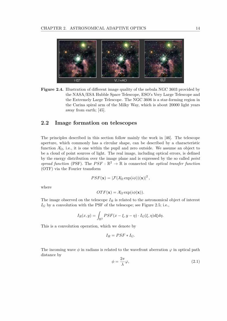
The ELT will have four first-light instruments; see Figure 2.3: the High Angular Reso-lution Monolithic Optical and Near-infrared Integral field spectograph (HARMONI), theMid-infrared ELT Imager and Spectograph (METIS), and the Multi-AO Imaging CAm-era for Deep Observations (MICADO) with the Adaptive Optics module Multi conjugateAdaptive Optics RelaY (MAORY). Having various instruments, the ELT makes observa-tions in a wide range of wavelengths possible, from optical to mid-infrared. The numeri-cal simulations within this thesis are carried out for a configuration similar to MAORY,which compensates for atmospheric turbulences over a 1 arc minute field of view in thenear-infrared regime. The correction is achieved using up to three deformable mirrorsthat are driven by a system based on several natural and laser guide stars. For a detaileddescription of the ELT and its instruments we refer to [45]. For the test specificationused throughout this thesis we refer to Chapter 7. Figure 2.4 reveals the excellent imagequality of the ELT based on the example of the nebula NGC 3603, which is about 20000light years away from the earth.
Figure 2.3. The ELT’s first-light instruments; [45].
CHAPTER 2. ASTRONOMICAL ADAPTIVE OPTICS 14
Figure 2.4. Illustration of different image quality of the nebula NGC 3603 provided bythe NASA/ESA Hubble Space Telescope, ESO’s Very Large Telescope andthe Extremely Large Telescope. The NGC 3606 is a star-forming region inthe Carina spiral arm of the Milky Way, which is about 20000 light yearsaway from earth; [45].
2.2 Image formation on telescopes
The principles described in this section follow mainly the work in [46]. The telescopeaperture, which commonly has a circular shape, can be described by a characteristicfunction XΩ, i.e., it is one within the pupil and zero outside. We assume an object tobe a cloud of point sources of light. The real image, including optical errors, is definedby the energy distribution over the image plane and is expressed by the so called pointspread function (PSF). The PSF : R2 → R is connected the optical transfer function(OTF) via the Fourier transform
PSF (x) = |F(XΩ exp(iϕ))(x)|2 ,
whereOTF (x) = XΩ exp(iϕ(x)).
The image observed on the telescope IR is related to the astronomical object of interestIG by a convolution with the PSF of the telescope; see Figure 2.5; i.e.,
IR(x, y) =∫R2PSF (x− ξ, y − η) · IG(ξ, η)dξdη.
This is a convolution operation, which we denote by
IR = PSF ∗ IG.
The incoming wave ϕ in radians is related to the wavefront aberration φ in optical pathdistance by
ϕ = 2πλφ, (2.1)

15 CHAPTER 2. ASTRONOMICAL ADAPTIVE OPTICS
for a certain wavelength λ. Note that within this thesis we omit the constant in Equa-tion (2.1) and use ϕ for the incoming wave as well as for the wavefront aberration,because we are only interested in the shape of the incoming wavefront aberrations.
If we neglect atmospheric perturbations and assume ϕ = 0, we obtain the so calleddiffraction limited PSF; see [47]. Assuming a circular telescope pupil with diameter Dwe get
PSF (x) = πD2
4λ2
(2J1(πD |x| /λ)πD |x| /λ
)2.
Here x ∈ R2, λ is the wavelength and J1 denotes the Bessel function of the first kind.This Bessel function can be represented by a series expansion around zero via
J1(x) =∞∑
n=0
(−1)n
n!Γ(n+ 2)
(x
2
)(2n+1),
where Γ(n) = (n− 1)! denotes the Gamma function for n ∈ N.
Figure 2.5. The PSF of the telescope relates the observed image IR with the astro-nomical object of interest IG; [48].
The PSF depends on the diameter D of the telescope. The larger the diameter of thetelescope the better its PSF approximates a delta distribution. Figure 2.6 illustrates atypical shape of a PSF. For ground based telescopes the PSF is affected by atmosphericturbulences. This results in oscillations that propagate outwards as well as a lowermaximum intensity. The goal in AO is to get as close as possible to the diffraction limitedPSF, because this results in a sharp image. Various PSF reconstruction algorithms forELTs exist; see [49–51].
2.3 Atmospheric turbulence
Atmospheric turbulences are caused by the irregular mixing of cold and hot air, trig-gered by the sun and wind. These irregularities make the refractive index of the airinhomogeneous, resulting in a distorted wavefront arriving at the telescope pupil. Theeffects of turbulence are non predictable, thus, they are typically modeled by a random

CHAPTER 2. ASTRONOMICAL ADAPTIVE OPTICS 16
Figure 2.6. Typical diffraction limited PSF; [48].
process. The refraction of the atmosphere in the random setting is given by the meanrefraction combined with some additive noise. Kolmogorov developed the fundamentalmodel for describing turbulence in the atmosphere.
2.3.1 Kolmogorov turbulence model
According to Kolmogorov [52] the behavior of the atmosphere is modeled via an isotropic,stationary random process. The representation of this random process is based on astructure function, which describes the expected difference of values at two points, andthe covariance function, which measures the spatial covariance. As we are dealing witha stationary process, both functions only depend on the separation ∆x of two pointsand not on a specific point x.
The structure function of a stationary process f is given by
Df (∆x) := E((f(x+ ∆x)− f(x))2),
and the covariance is defined via
Cf (∆x) := E((f(x)− E(f))(f(x+ ∆x)− E(f))).
The power spectral density (PSD) characterizes the behavior of the covariance functionin the Fourier domain and is defined by
Φf (∆x) := E((f(x)− E(f))(f(x+ ∆x)− E(f))).
Kolmogorov’s theory is limited by te two quantities l0 and L0 called inner and outerscale. The inner scale represents the size of the smallest eddy in the turbulence, whereas

17 CHAPTER 2. ASTRONOMICAL ADAPTIVE OPTICS
the outer scale corresponds to the largest size. Within this range, Kolmogorov statedthat the structure function of the refractive index of the atmosphere at a certain heighth is given by
Df (∆x) := c2n(h)|∆x|2/3 for l0 < |∆x| < L0,
where c2n(h) denotes the refractive index structure function. This quantity measures
the turbulence strength at a certain altitude h. It is usually measured empirically anddepends on weather conditions. The PSD of the refractive index n is then given by
Φn(κ) := 0.033C2n(h)|κ|−11/3 for 2πL−1
0 < |κ| < 2πl−10 ,
where κ = (κ1, κ2, κ3) is the spatial frequency and |κ| denotes the Euclidean norm. Fora very small |κ| → 0, i.e., for turbulent eddies larger than the outer scale, Kolmogorov’smodel shows problems due to a singularity. To overcome this unwanted effect, the vonKarman model was introduced.
2.3.2 Von Karman turbulence model
The von Karman model [53] modifies the Kolmogorov model in order to overcome theproblem with the singularity at κ = 0. This leads to the following, slightly modifieddefinition of the power spectral density
Φf (κ) = 0.033C2n(h)
(|κ|+ κ20)11/6 exp
(−|κ|
2
κ2m
),
with κ0 = 2πL−10 and κm = 5.92l−1
0 . For |κ| → 0 the PSD in the von Karman turbulencemodel has a finite value.
2.3.3 Turbulence layers
Most of the atmospheric turbulences are concentrated in separate layers, which travelat a certain velocity parallel to the surface of the earth; see [54]. These turbulentpatterns change slower than the wind speed, thus, for a short time frame constantso called c2
n profiles can be assumed; see [55]. During the day, the turbulences aretypically stronger near the earth’s surface, whereas during the night perturbations arestronger at higher altitudes; see [56]. The atmosphere can be modeled by L statisticallyindependent turbulent layers, which are infinitely thin; see [57]. The optical strength ofthe atmospheric turbulence at a certain layer l = 1, ..., L at height hl is given by c2
n(hl).In fact, a small number of layers is sufficient, as shown, e.g., in [48, 58, 59]. Withinour numerical simulations we consider between 3 and 9 layers, derived by ESO frommeasurements at their site in the Atacama desert in Chile. These seeing conditions are

CHAPTER 2. ASTRONOMICAL ADAPTIVE OPTICS 18
derived from c2n profiles, wind speeds and layer altitudes. They are described by the
isoplanatic angle θ0 and the Fried parameter r0. For the detailed parameters we refer toChapter 7.
The Fried parameter r0 assesses the seeing conditions with respect to a certain wave-length λ. Typically, the parameter is defined in the visible, i.e., at 500 nanometersby
r0 = 0.185 ·(
λ2∫∞0 c2
n(h)dh
)3/5
;
see [60]. The atmospheric seeing β is the ratio between the wavelength and the Friedparameter:
β = λ
r0.
The Fried parameter lies within 10 and 20 centimetres for the visible region of the spec-trum. Larger values correspond to good seeing conditions, and thus to weak turbulence,whereas smaller values refer to bad seeing and strong perturbations.
Within AO we use measurements from guide stars as reference sources to correct thedistorted wavefronts of other nearby objects of interest. In general, these measurementsare only valid for objects in the same direction as the guide star. If the angle betweenthe reference source and the object of interest increases, the error in the wavefrontbecomes uncorrelated. We denote by θ0 the angle at which two speckle images start tolook different; see [56]. Angular anisoplatism is the effect when the angle between twoobjects is bigger than θ0. For an observation at a guide star direction θ, the variance ofphase is given by
E(σ2ϕ) =
(θ
θ0
).
Assuming a single layer atmosphere at altitude h, the isoplanatic angle is given by therelation between the Fried parameter and the layer height by
θ0 = 0.31r0h.
For more details we refer to [55, 56, 61].
2.4 AO components
AO [60, 62, 63] is a technique to compensate the rapidly changing optical distortionsin the atmosphere, that heavily degrade the image quality of earthbound telescopes.The correction process is commonly split into two parts. First, the deformations of

19 CHAPTER 2. ASTRONOMICAL ADAPTIVE OPTICS
wavefronts emitted by natural or laser guide stars in the vicinity of the object of interestare measured via WFSs. This information is then used by a reconstruction algorithmto calculate the actuator commands that deform the mirror. Finally, the light fromguide stars as well as the observed object is reflected onto the deformable mirror and thedistortions get removed. Figure 2.7 illustrates the basic design of an AO system runningin closed loop. The incoming wavefront which got distorted when passing through theturbulent atmosphere, reaches the DM and gets corrected. A so called beam splitter(BS) splits the light into two parts. One part is propagated to the scientific cameraand the other to the WFS. These already corrected sensor measurements are used tocompute the actual mirror commands for the next incoming wavefront.
Figure 2.7. Basic design of an AO system.
The main components of an AO system are guide stars, wavefront sensors and deformablemirrors. In the following subsections we describe these components in greater detail.
2.4.1 Guide stars
Guide stars (GS) are bright objects, which serve as point light sources. We differentiatebetween natural guide stars (NGS), i.e., real astronomical objects, and laser guide stars(LGS) that are artificially generated by a laser beam.

CHAPTER 2. ASTRONOMICAL ADAPTIVE OPTICS 20
Natural Guide Star
An NGS is a bright star that serves as a reference point for the WFS to detect atmo-spheric distortions. The star is modeled as a point source at an infinite height. Assuminga layered atmospheric model, the wavefront aberrations in the direction θ of an NGS aregiven by
φθ(x) = (PNGSθ ϕ)(x) :=
L∑ℓ=1
ϕl(x+ θhℓ), (2.2)
where ϕℓ is the turbulent layer at altitude hl for ℓ = 1, ..., L. We call PNGSθ the geometric
propagation operator in the direction of the NGS.
We assume that the photon noise from the NGS, that affects the WFS measurements,is modeled by a Gaussian random variable with zero mean and covariance matrix Cη.The noise is identically distributed in each subaperture and the x- and y-measurementsare uncorrelated. Hence, the covariance matrix can be defined by
Cη = σ2I, (2.3)where σ2 is the noise variance of a single measurement. It is given by
σ2 = 1nphotons
, (2.4)
where nphotons is the number of photons per subaperture.
Laser Guide Star
For an LGS the model is more complex. An LGS is generated by a powerful laser beam.In this thesis we consider so called sodium LGSs. Besides this kind of LGSs so calledrayleigh LGSs are frequently used; see [62] for details. For sodium LGS the laser beamscatters in the sodium layer, at which the light is then backscattered and sensed by theWFS. These procedure induces some important effects that have to be taken into accountwhen modelling an LGS: the cone effect, spot elongation and tip-tilt indetermination.
In contrast to the infinite height assumed for an NGS, an LGS is considered to be ata finite height H. Due to the finite altitude, the light detected by the telescope passesthrough a cone-like volume of the atmosphere; see Figure 2.8. This behavior is referredto as the cone effect.
As for NGS we assume a layered model of the atmosphere. The incoming wavefrontaberrations in the direction θ of an LGS are given by
φθ(x) = (PLGSθ ϕ)(x) :=
L∑ℓ=1
ϕl((1−hℓ
H)x+ θhℓ), (2.5)

21 CHAPTER 2. ASTRONOMICAL ADAPTIVE OPTICS
Figure 2.8. Cone effect for LGS; [48]. Due to the finite height of the LGS, the lightpasses through a cone volume.
where PLGSθ is called the geometric propagation operator in the direction of the LGS.
As the sodium layer has a certain layer of thickness, the scattering of the laser beamhappens in a vertical stripe instead of in a single point. Thus, the sodium layer thicknessmust be considered when modeling the photon noise. The charge-coupled device (CCD)detector of the WFS observes this stripe as an elongated spot. The effect is commonlyknown as spot elongation and is illustrated in Figure 2.9.
Figure 2.9. Spot elongation for LGS; [48].
The vertical density profile of the laser beam scatter is modeled by a Gaussian randomvariable with mean H and the full width at half maximum (FWHM) of the sodium

CHAPTER 2. ASTRONOMICAL ADAPTIVE OPTICS 22
density profile in meters, which is defined by
FWHM = 2√
2ln(2)σ.
Further, we define the laser launch positions as (xLL1 , xLL
2 ) and the midpoint of a sub-aperture Ωij by (xi, xj) with
xi = xi + xi+12 ,
for 0 ≤ i < ns where the xi are given by Equation (2.8).
The elongation vector in a subaperture Ωij is given by
βij = (βij,1, βij,2) = FWHM
H2
((xi, xj)− (xLL
1 , xLL2 )
).
The spot elongated noise covariance matrix in a subaperture is given by
Cij = σ2(I +
α2η
f2
(β2
ij,1 βij,1βij,2βij,1βij,2 β2
ij,2
)),
where I denotes the identity matrix, σ is defined as in (2.4), f is the FWHM of thenon-elongated spot. To cope with noise sources that are not included into the modelabove, e.g., read out noise, we introduce the fine-tuning parameter αη. If αη = 0 themodel coincide with the NGS model, whereas for αη = 1 we have the full LGS model.
Summarized, the noise model for a WFS associated to an LGS is given by a Gaussianrandom variable with zero mean and covariance matrix
Cη = diag(Cij), (2.6)
with 0 ≤ i, j < ns for an active subaperture Ωij .
In every AO system at least one NGS has to be used in order to overcome the problemof tip-tilt indetermination. The laser beam passes through the atmosphere twice, oncewhen traveling up to the sodium layer and once when being scattered from this sodiumlayer. Hence, the real position of the LGS is unknown as tip or tilt modes cannot bedetermined. This leads to an uncertainty in the position of the spots of the ShackHartman sensor and, subsequently, to untrustworthy low-order aberrations of the LGS.Figure 2.10 illustrates this behavior.
Although the low-order information is unreliable, the relative motion of the spots withinthe subapertures is kept, and thus also the high-order aberrations. Note that froma measurements point of view, the tip-tilt uncertainty is nothing else than incorrectaverage slopes over the pupil of the telescope. To achieve a good correction of theincoming wavefronts it is essential to determine the tip-tilt aberrations. Thus, the LGS

23 CHAPTER 2. ASTRONOMICAL ADAPTIVE OPTICS
Figure 2.10. Tip-tilt indetermination for an LGS; [48].
are coupled with at least one NGS that senses the low-order tip-tilt modes. In this case,a so called low-order tip-tilt sensor (TTS) is used that has typically a much smaller sizeof, e.g., 2 × 2 or 1 × 1 subapertures. These two sensors can either be assigned to twodifferent mirrors, one for high-order modes and one for tip-tilt correction, or the twoproblems can be combined. Throughout this thesis we use the second approach, i.e., theNGS and the LGS problem are coupled.
2.4.2 Deformable mirrors
A deformable mirror (DM) typically consists of a thin surface which reflects the light,and a set of actuators that deform the mirror. Here, we assume a simple model of abilinear DM, i.e., the shape is described using a piecewise continuous bilinear function,which we denote by a.
We define the domain on which the DM operates by
Ω := [−D/2, D/2]2, (2.7)
where D is the telescope diameter. Further, we denote by n2a the number of actuators
or nodal points of the piecewise bilinear function. We assume that these points arearranged in a rectangular grid with a spacing of d := D/(na − 1). Since the telescopehas a circular shape, not all of these actuators are active, i.e., they have no effect on thecorrection of the wavefront.

CHAPTER 2. ASTRONOMICAL ADAPTIVE OPTICS 24
The actuator positions are given by (xi, xj) for 0 ≤ i, j ≤ na, where
xi := −D/2 + i · d.
The actuator grid is then given by the set of points
(xi, xj) : 0 ≤ i, j < na.
Moreover, we define the square sub-domains of Ω by
Ωij := [xi, xi+1]× [xj , xj+1].
To each subdomain a bilinear function defined on [0, 1]2 is associated by
bij(x, y) = aij(1− x− y + xy) + ai,j+1(x− xy) + ai+1,j(y − xy) + ai+1,j+1xy,
where the values aij are called actuator commands.
Figure 2.11 shows different types of DMs. The simplest mirror, which is considered asa low risk concept, is called segmented DM. This mirror has only up to three degrees offreedom (two axes for tilt and piston), but a wide dynamic range and a good frequencyresponse. Due to the gaps between the segments diffraction effects arise. Moreover, sucha DM has a higher fitting error compared to other types. The face-sheet DM is stableover time and changes in temperature due to its continuous faceplate. The drawbackof this DM type is the limited stroke. This stroke limitation is induced by the stress inthe faceplate, which arises due to actuator motion. The deformable mirror of the ELTcalled M4 consists of a segmented and thin shell. The mirror is driven at 500 Hertz byabout 5300 actuators. For the numerical simulations carried out in the framework ofthis thesis we assume the Fried geometry with equidistant actuator spacing for the DMs,as described in [64].
In general, one distinguishes between the shape of the DM and the mirror commands,which deform the DM. Throughout this thesis we use both wordings to denote the mirrorcommands a.
2.4.3 Wavefront sensors
A wavefront sensor (WFS) measures indirectly the distortions of the wavefronts usingthe light from an NGS or an LGS. Various WFSs are used within AO. In the following,we describe the Shack-Hartmann (SH) WFS and the pyramid WFS in more detail. Forthe numerical simulations carried in this thesis we restrict ourselves to the SH WFSmodel.

25 CHAPTER 2. ASTRONOMICAL ADAPTIVE OPTICS
Figure 2.11. Different types of DMs; [65].
Shack-Hartmann WFS
A Shack-Hartmann (SH) WFS; see [63, 66, 67]; consists of a quadratic array of smalllenslets and a CCD photon detector lying behind this array. The vertical and horizontalshifts of the focal points determine the average slope of the wavefront over the area of thelens, known as subaperture. Similar as for the actuators we introduce the subaperturegrid. Let
Ω := [−D/2, D/2]2,be the domain on which the wavefront is defined. Here D denotes again the diameter ofthe telescope. Further, we denote by n2
s the number of subapertures. As for the DM, notall subapertures need to be active. Because the telescope pupil has a circular shape, notall subapertures are illuminated. The subaperture grid consists of a set of equidistantlyspaced points and is given by
(xi, xj) : 0 ≤ i, j ≤ ns, where xi := −D/2 + i · d. (2.8)
A subaperture is then defined as an open square sub-domain of Ω by
Ωij := (xi, xi+1)× (xj , xj+1).
Within a subaperture Ωij the SH measurements are modelled as the average slopes ofthe wavefront aberration φ and given by
sxij = 1
d2
∫Ωij
∂φ
∂x(x, y)d(x, y), (2.9)
syij = 1
d2
∫Ωij
∂φ
∂y(x, y)d(x, y), (2.10)

CHAPTER 2. ASTRONOMICAL ADAPTIVE OPTICS 26
Figure 2.12. SH WFS with 7× 7 subapertures. An active subaperture Ωij is indicatedby continuous borders, whereas a non-active subaperture is surroundedby dashed lines; [23].
where s := (sx, sy) are the average slopes in x and y-direction, respectively, and d2
is the area of the subaperture Ωij . We assume that the incoming wavefront aber-ration φ is approximated by a continuous piecewise bilinear function φij at points(xi, xj) : 0 ≤ i, j ≤ ns. Then Equation (2.9) reduces to
sxij = (φi,j+1 − φi,j) + (φi+1,j+1 − φi+1,j)
2 , (2.11)
syij = (φi+1,j − φi,j) + (φi+1,j+1 − φi,j+1)
2 ; (2.12)
see [68]. In this work we denote the SH measurement vector by s = (sx, sy). The vectorssx and sy are a concatenation of values sx
ij and syij for (i, j) a set of indices that belongs
to an active subaperture Ωij . The subapertures where no measurements are available areexcluded from s. To the above defined relation between measurements s and wavefrontaberrations φ we associate a SH WFS operator, which we denote by Γ = (Γx,Γy). Here,Γx and Γy determine the slopes in x- and y-direction, respectively,
s =(sx
sy
)=(
ΓxφΓyφ
)= Γφ. (2.13)
The CCD detector senses photons over a certain time frame. Typically, the SH WFSsuffers from read-out noise and photon noise. The read-out noise is due to errors inreading photons by the CCD detector planes. This kind of noise is measured in electronsper pixel. The photon noise is related to the number of photons that are sensed by theCCD in a subaperture during a certain time frame. If we are dealing with a very faintlight beacon, too few photons are detected by the sensor. This leads to an inaccurateposition of the focal point in the subaperture. The photon noise is modelled by a poissonprocess. For a large number of photons, the noise can be approximated by a Gaussianrandom variable.

27 CHAPTER 2. ASTRONOMICAL ADAPTIVE OPTICS
Pyramid WFS
The main component of the pyramid WFS is a four-sided glass pyramidal prism in thefocal plane of the telescope; see, e.g., [69] . This prism splits the incoming light intofour beams. The relay lens, located behind the prism, re-images the beams leadingto four different images I1, I2, I3 and I4 on the CCD camera; see Figure 2.13. Similarto SH WFSs, pyramid WFS measurements are given on a grid of subapertures; seeEquation 2.7. The sensor measurements in x- and y-direction are given by
Sx(x, y) = (I1(x, y) + I2(x, y))− (I3(x, y) + I4(x, y))I0
, (2.14)
Sy(x, y) = (I1(x, y) + I4(x, y))− (I2(x, y) + I3(x, y))I0
, (2.15)
where I0 denotes the average intensity; see [70].
Figure 2.13. Pyramid WFS; [69].
It might happen that the incoming beam is not exactly focused on the spot of the pyra-midal prism. Hence, light does not fall on every side of the pyramid. To overcome thisbehavior, the spot of the pyramid can be modulated. The modulation of the incomingbeam allows a linearisation of the sensor and to increase its dynamic range; see [70–72].Several possibilities exist to dynamically modulate the beam; see, e.g., [69, 73]. Theadvantage of the pyramid WFS over the SH WFS is the increased sensitivity which en-ables the usage of fainter stars and higher sky coverage; see [74]. For recent researchon the pyramid WFS, especially on new mathematical models and accurate wavefrontreconstruction, we refer to [75–79].
The four-sided pyramidal prism of the sensor can be approximated via 2 orthogonallyplaced two-sided roof prisms. Each of the roofs creates two different images on the

CHAPTER 2. ASTRONOMICAL ADAPTIVE OPTICS 28
detector. The sensor measurements Sx and Sy are obtained by subtracting the twointensity patterns. Due to the physical decoupling of the prisms, the measurementscontain information only in x− or y−direction, respectively.
2.5 AO systems
Depending on the specific aim of the system, i.e., observing one or several objects ofinterest or correcting for a wide field of view, the number of NGS and LGS involved in thecorrection change. This is what is referred to as different operating modes. Figure 2.14shows the 4 operating modes considered throughout thesis. In the following subsectionswe describe these AO systems in more detail.
Figure 2.14. The different AO operating modes; [48]. The red or green stars indicatenatural or laser guide stars. The blue parts refer to the corrected areasand the violet spirals are the objects of interest.
2.5.1 Single Conjugate AO
If the object of interest, e.g., a star or a galaxy, is located near a bright NGS, the classicalAO system Single Conjugate AO (SCAO) is used. In a SCAO system the wavefront isreconstructed using one WFS that measures the deformations, and one DM, where theshape is chosen according to the reconstruction algorithm; see Figure 2.15(a). Thedrawback of a SCAO system is, that the further away the object of interest is from theNGS, the worse the correction of the wavefront becomes. In the general case, an NGSnear the object of interest is not available.
2.5.2 Laser Tomography AO
If no NGS is available in the vicinity of the object of interest, the usage of a SCAOsystem is not possible. The idea is to use a laser beam to generate one or more LGSs

29 CHAPTER 2. ASTRONOMICAL ADAPTIVE OPTICS
to obtain a good correction. The LGSs are combined with at least one NGS to correctfor the low-order modes; see Section 2.4.1; which are not available using LGS only. Ingeneral, a combination of several LGS and NGS is possible.
Figure 2.15. Figure(a) illustrates a SCAO system using one NGS to correct for onedirection of interest is shown. Figure(b) shows an LTAO system withtwo guide stars that corrects for the direction of one object of interest isillustrated; [48].
Within the framework of a Laser Tomography AO (LTAO) a number of GLGS and GNGS
are used in combination with a single mirror to reconstruct the wavefront. Figure 2.15(b)illustrates an LTAO system. The correction is performed through two steps. The firststep is called atmospheric tomography, where the turbulent layers are reconstructed fromsensor measurements. In the second step, the shape of the DM is chosen according to theprojection of the wavefront through the reconstructed layers in the direction of interest.For an SCAO system, the reconstructed layer is located at the altitude of the DM, hence,the grid points of the reconstructed layer are aligned with the mirror nodal values andnothing has to be done. For an LTAO system, the mirror is optimized towards a certaindirection of interest θ1. Thus, the DM has to be fitted to the reconstructed layers. Thisfitting step is defined by a projection through the reconstructed layers towards θ1
a1 = [PNGSθ1,1 · · ·PNGS
θ1,L ]
⎛⎜⎝ϕ1...ϕL
⎞⎟⎠ ,where PNGS
θ1,ℓ is a bilinear interpolation onto layer ℓ = 1, ..., L towards the direction θ1.

CHAPTER 2. ASTRONOMICAL ADAPTIVE OPTICS 30
2.5.3 Multi Object AO
In contrast to LTAO, Multi Object AO (MOAO) corrects for multiple directions of in-terest simultaneously sby using several mirrors; see Figure2.16(a). Each mirror correctsfor a specific direction. As in the LTAO case, a combination of NGS and LGS is usedfor reconstructing the layers. Since we are optimizing towards M directions of interestθ1, ..., θM , instead of only one, this leads to a slightly different mirror fitting step⎛⎜⎝ a1
...aM
⎞⎟⎠ =
⎛⎜⎜⎝PNGS
θ1,1 · · · PNGSθ1,L
......
PNGSθM ,1 · · · PNGS
θM ,L
⎞⎟⎟⎠⎛⎜⎝ϕ1
...ϕL
⎞⎟⎠ .
2.5.4 Multi Conjugate AO
Like an MOAO system, a Multi Conjugate AO (MCAO) system corrects for multipledirections, however, with the aim to achieve a uniformly good correction over the wholeFoV and not into specific directions. For a graphical illustration see Figure 2.16(b). Forthat purpose, several DMs are used conjugated to different heights in the atmosphere.As for LTAO and MOAO systems, the atmospheric tomography problem is solved in afirst step. In the second step, the shapes of the M mirrors are fitted to the reconstructedlayers in order to optimize the quality in a large FoV. The standard approach for mirrorfitting; see e.g. [63]; is to minimize the following functional∫
F oV
∫ΩM
(PNGS
ϕ ϕ)(x)− (PNGSϕ a)(x)
2dxdϕ,
where ϕ = (ϕ1, ..., ϕL) is the vector of layers and a = (a1, ..., aM ) is the vector of mirrorshapes. For details we refer to [80]. By ΩM we denote the telescope pupil and FoV isa set of directions in the FoV. The operators PNGS
ϕ and PNGSϕ are projections through
layers and DMs, respectively.
For more details on the fitting step for different AO systems we refer to [81].
2.6 AO delay and control
There is a certain delay between the time when the measurements are obtained fromthe WFSs and the time when the wavefronts get corrected by the DMs. Because theatmosphere changes rapidly, the AO system updates the DM shapes based on the currentmeasurements, collected by the WFSs, and the previous DM shapes; see [82]. We denote

31 CHAPTER 2. ASTRONOMICAL ADAPTIVE OPTICS
Figure 2.16. Figure(a) illustrates an MOAO system correcting for two objects of inter-ests using two DMs is shown. Figure (b) shows an MCAO system, thatachieves a good correction in a wide FoV, using two DMs conjugated totwo different altitudes; [48].
the previous, the current and the next time step of the loop by the superscript indices (i−1), (i) and (i+1). The superscript indices (i−1, i) and (i, i+1) denote the measurementsbetween the respective time steps. In this thesis we consider a two-step delay; see, e.g.,[23]. The new mirror shapes a(i+1) are determined from the reconstruction that uses themeasurements s(i−1,i) and from the previous mirror shapes a(i). Because of the delay,the measurements s(i,i+1) are not available at time step (i + 1) for the reconstruction.See Figure 2.17 for a graphical representation.
a(i)a(i−1) a(i+1)
s(i,i+1)s(i−1,i)i − 1 i i + 1
Figure 2.17. Two-step delay of an AO system. WFS measurements are obtained be-tween (i− 1, i) and the correction is applied in the interval (i, i+ 1). DMshapes are adapted in (i−1, i) and (i+1). The measurements s(i,i+1) arenot available at step (i+ 1) (indicated in gray).
We denote the average wavefront aberrations in the interval (i− 1, i) by φ(i−1,i) and theslope measurements obtained in this interval by s(i−1,i). In the time frame (i, i+ 1) thenumerical reconstruction algorithms determine the mirror shapes based on s(i−1,i) andin time step (i + 1) the DM is updated. There are two ways on how to align the DMand the corresponding WFS in the optical path of an AO system. If the AO system isconfigured such that the WFS is installed before the DM, the measurements are obtaineddirectly from the wavefronts by
s(i−1,i) = Γφ(i−1,i) + η,
where Γ is the SH operator and η is the measurement noise. This control scheme iscalled open loop. In Figure 2.7 a closed loop control is shown, i.e., the DM is installed

CHAPTER 2. ASTRONOMICAL ADAPTIVE OPTICS 32
before the WFS in the optical path, thus, the wavefronts are already corrected beforeobtained from the WFS. The measurements s(i−1,i) correspond to the residuals of thecorrected wavefronts minus the DM correction
s(i−1,i) = Γ(φ(i−1,i) − a(i−1)) + η. (2.16)
2.7 AO measures
In the following sections we briefly describe some important AO quantities often re-ferred to within this thesis. Moreover, we define a quantity for measuring the qualityof the reconstruction algorithms presented in this thesis, which is frequently used in thecommunity of AO.
2.7.1 Important quantities
Wavelength
For the simulations contained in this thesis we consider observations in the near infrared,i.e., in the K-band, which denotes a wavelength λ between 2.0 µm and 2.4 µm. Theastronomical band for sensing and evaluating can be different. Note that a differentwavelength λ can change the performance of an AO system significantly.
Field of View
The field of view (FoV) is commonly indicated by the diameter of a circle (in arcmin orarcsec). One distinguishes between the corrected FoV, which is determined by the GSasterism, and the scientific FoV. Throughout this thesis we refer by FoV to the correctedFoV.
Photon flux
To measure the intensity of light that reaches the telescope pupil the number of photonsnphotons for one subaperture of a WFS per frame is used. We differentiate between highand low photon flux. In general, up to 500 photons is called low photon flux, whereasmagnitudes of 10000 are referred to as high photon flux. However, the threshold dependsheavily on the signal-to-noise-ratio.

33 CHAPTER 2. ASTRONOMICAL ADAPTIVE OPTICS
Sensor noise
The most dominant error sources within AO are the photon noise and the read-out noise.The photon noise, which is described by the signal-to-noise-ratio, denotes the noise inthe sensor output. It depends on the sensor size, the number of pixels, the photonflux and the number of subapertures. The read-out noise is triggered by unpredictablephenomena and latency within the read-out process of the CCD detector. We combineall error sources into one probabilistic quantity η. Hence, the model for obtaining themeasurements from the WFS becomes
s = Wφ+ η.
Within the framework of this thesis we consider W to be the SH operator Γ. The usageof regularization methods helps in keeping the error propagation low.
Frame rate
The time in which the CCD detector is sensing the photons is called frame rate andgiven in Hertz. In our simulations the frame rate lies at about 500 Hertz, i.e., 2 ms. Thetomographic reconstruction has to be performed in approximately half the time.
2.7.2 Quality evaluation: Strehl ratio
The Strehl ratio is a frequently used quality evaluation criterion within AO. The shortexposure (SE) Strehl is defined as the ratio between the maximum of the real energydistribution of incoming light in the image plane I(x, y) over the hypothetical distributionID(x, y), which stems from the assumption of diffraction-limited imaging,
S :=max(x,y) I(x, y)
max(x,y) ID(x, y) ∈ [0, 1].
The higher the Strehl ratio the better the quality of the AO system. The maximumof 1 is reached only in the diffraction-limited case. A tip-tilt mode, which leads to ahorizontal shift of I(x, y), does not influence S. In order to detect a tip-tilt mode, thelong exposure (LE) Strehl ratio is used. The LE Strehl represents the quality of theimage from the start of the loop until a certain time step. The short and long exposureStrehl ratios are commonly indicated in %. For more details about the Strehl ratio werefer to [62].


Chapter 3
Real-time systems
Within a real-time computing system the correctness of a certain calculation dependsnot only on the value of the result, but also at which time frame it is available. Areal-time system must respond in a predictable amount of time. Moreover, such systemsneed sufficient computational power to meet the timing and processing requirements ofthe specific real-time application, such as the control of an AO system. The main partsof this chapter are based on the book in [83].
A real-time system can be classified into hard real-time (HRT) and soft real-time (SRT)systems. HRT systems have a strict predefined deadline where the results must be avail-able to guarantee that everything works properly. For SRT systems there is a specifiedlevel of urgency and the system executes the task with highest priority. Within theframework of AO, HRT is related to the computation of the DM commands from sensormeasurements, which is typically at 500−1000 Hz. SRT is related to the pre-computationof matrices whenever certain parameters at the telescope or in the atmosphere change.For our test configuration the SRT is at 6 minutes. In general, the time frame of HRTis much smaller than that of SRT.
3.1 Hardware architecture of AO systems
In general, three basic hardware technologies are used for the real-time control of largetelescopes: Central Processing Units (CPUs), Graphics Processing Units (GPUs), andField Programmable Gate Arrays (FPGAs). In the following, we provide an overviewon all of them. In Chapter 9 we decide which hardware is suitable for which algorithm.Our decision relies on a theoretical performance analysis of the wavefront reconstructionalgorithms for ELT-sized test configurations. We follow here the work in [40] for CPUs,
35

CHAPTER 3. REAL-TIME SYSTEMS 36
[41] for GPUs and [84] for the FPGA technology.
3.1.1 Central processing units
The most widespread processing units, and thus the most straightforward way to imple-ment a real-time control architecture, are Central Processing Units (CPUs). Internally,a CPU consists of several billion transistors. The number of transistors can serve as arough estimate for the computational performance. Another performance factor is theclock frequency, which determines the time a processor needs for one cycle, and hencethe time to execute a single instruction. Traditionally, a CPU carries out instructions onthe data in a sequential way. However, nowadays CPUs consists of several independentprocessor cores. All cores of a multicore processor can execute tasks simultaneously,which leads to parallel execution. In order to coordinate the control flow of the cores,parallel programming techniques are required. All cores of a processor can access thesame global memory and share caches that store frequently used data with a very fastdata access compared to global memory. Caches are arranged in different levels, start-ing from small, fast and expensive L1 cache up to slower but larger L2, L3 cache andglobal memory. Access of data in L1 cache takes about 2-4 clock cycles, whereas accessto global memory can take hundreds of cycles. Generally, CPUs are managed by theoperating system (OS). These OS often generate unintended side effects in latency, jitterand determinism of the control behavior; see [85].
For programming on CPUs we use the language C++, which was invented by BjarneStroustrup in 1979 as an extension to C; see [86]. C++ became very popular for applica-tions were the computational efficiency is essential. It offers a valuable way for hardwareoriented programming while still providing high level programming constructs. For com-piling C++ code we utilize the GNU Compiler Collection (GCC); see [87].
3.1.2 Graphics processing units
A Graphics Processing Unit (GPU) is optimized for rapid processing of simple tasks.Due to their highly parallel structure, GPUs outperform CPUs by orders of magnitude inalgorithms where a huge amount of data has to be processed in parallel. The host CPUdirects tasks to the GPU via a stream through a graphics pipeline. A GPU device has ascalable array of multithreaded Streaming Multiprocessors (SMs), each having a fixed setof processing cores. Each multiprocessor can execute hundreds of threads concurrentlyusing an architecture called Single-Instruction, Multiple-Thread (SIMT). The multipro-cessor creates, manages, schedules, and executes parallel threads in groups of 32, calledwarps. Each warp executes one instruction at a time. All instructions are pipelined,within a single thread instruction level parallelism is performed and thread level paral-

37 CHAPTER 3. REAL-TIME SYSTEMS
lelism is implemented through concurrent hardware multithreading. To coordinate thiscontrol flow parallel programming languages, such as CUDA, are used. For more detailson CUDA we refer to Section 3.3.2. In general, a GPU has 3 types of physical memory:register memory, shared memory and global memory. Register memory (256 kB) andshared memory (48 kB) reside on chip and are fast in access, whereas global memoryis usually several gigabytes, located off chip and is slow in access. As for CPUs, someunintended side effects in latency, jitter and determinism of the control behavior can beobserved for GPUs as well; see [85].
Figure 3.1 shows a schematic illustration of the CPU and GPU architectures. Theabbreviation ALU (white) denotes the arithmetic logic unit, which is a digital circuitperforming arithmetic and bitwise operations. GPUs have a much higher memory band-width compared to CPUs, because more transistors are dedicated to data processingrather than caching (light gray) or flow control (dark gray). This explains why GPUsare extremely efficient for highly parallel computations, such as graphics rendering. Theyhide memory access latencies with computational throughput. In contrast, for the CPUmemory access latencies are avoided through large data caches and flow control.
ControlALU
ALU ALU
ALU
Cache
DRAM
CPU
DRAM
GPUFigure 3.1. Schematic illustration of CPU and GPU architecture consisting of ALUs
(white), flow control (dark gray), caches (light gray) and DRAM. The GPUdedicates more transistors to data processing.
3.1.3 Field programmable gate arrays
A Field Programmable Gate Array (FPGA) is an array of logic gates that can be con-figured by the programmer. Common functions, e.g., addition and multiplication, areimplemented by interconnected digital subcircuits. These subcircuits, also called Con-figurable Logic Blocks (CLBs), build the core of the FPGAs programmable logic andprovide boolean as well as arithmetic operations and data storage. Moreover, an FPGAcontains so called I/O blocks, which consist of components that allow the communica-

CHAPTER 3. REAL-TIME SYSTEMS 38
tion between CLBs and other blocks on the board. Figure 3.2 illustrates a schematicrepresentation of the design of an FPGA. The two most dominant FPGAs manufacturerare Xilinx and Intel (former Altera). An FPGA is designed to be reconfigured by a pro-grammer many times after it was manufactured. This is the reason why they are calledfield programmable. In contrast to that, ASICs (Application Specific Integrated Cir-cuits) are fixed circuits executing a certain task. The production of such ASICs is veryexpensive, thus, the idea behind FPGAs is to provide fixed hardware, but a configurablefunctionality.
Figure 3.2. Schematic design of an FPGA.
In general, FPGA development is considered to be more difficult than programmingmicro controllers. However, FPGAs are always supported by software that convertsyour hardware design into programmings bits. The two most common programminglanguages for FPGA are called Verilog and Very High Speed Integrated Circuit HardwareDescription Language (VHDL). For more details we refer to [84].
3.2 Pipelining
For the control of a large AO system pipelining is used to increase the computationalthroughput. In a pipelined system the processor is working on different tasks at thesame time by overlapping instructions, as illustrated for a simple example in Table 3.3.

39 CHAPTER 3. REAL-TIME SYSTEMS
Instead of six clock cycles used for the non pipelined instructions 1 and 2, only four clockcycles are required when using pipelining.
cycle 1 cycle 2 cycle 3 cycle 4 cycle 5 cycle 6
Instr. 1 Fetch Decode Execute
Instr. 2 Fetch Decode Execute
Pip. Instr. 1 Fetch Decode Execute
Pip. Instr. 2 Fetch Decode Execute
Table 3.3. Cycle without (Instr. 1 and Instr. 2) and with (Pip. Instr. 1 and Pip.Instr. 2) pipelining.
This simple concept is very efficient also for AO systems. The measurement vector sis obtained in HRT from the WFS and used to calculate the mirror commands with areconstruction algorithm. However, due to the latency from the data acquisition from thesensors, s is not available at once. Hence, for operations that do not require the completevector the computation can be started before the whole vector is available. This leads toan overlap of the time frame required for the data transfer and the one for calculation,and thus speeds up the overall computational performance. As an example we considerhere the computation of pseudo open loop measurements; see also Equation (2.16);
s← s+ Γa(i−1),
where Γ denotes the SH matrix and a(i−1) is the DM shape of the previous time step.When closed loop control is applied this computation is done as a first step of a recon-struction algorithm, before the tomographic reconstruction takes place. The measure-ment vector here is only required for the final sum and computing the sum of two vectorsis perfectly pipelineable. Thus, as soon as elements of s are accessible, the first elementsof the result vector can be calculated.
3.3 Parallelization
Without parallelization it would not be possible to meet the real-time requirements of alarge AO system as, e.g., required for the ELT. Therefore, we provide a rough overviewover several parallel programming approaches for CPUs, GPUs and FPGAs. Again, wefollow the work in [40, 41, 84].

CHAPTER 3. REAL-TIME SYSTEMS 40
3.3.1 Thread programming on CPU
A thread model in which all threads have access to shared variables is a common parallelprogramming model for multi-core platforms with a shared address space. The sharedvariables are used to exchange data. Below, we describe two popular environments forthread programming: Pthreads and OpenMP.
POSIX threads (Pthreads) is a standard, based on the programming language C, forthread-based programming. All data types, interfaces and macros related to Pthreadsare available via a header file. The globally shared address space can be accessed by allthreads of a process. In addition, each thread has a separate runtime stack to store localvariables. To utilize Pthreads, a programmer has to identify parts of the program thatcan be executed concurrently and create a suitable number of user threads. This userthreads are mapped by the scheduler of the library to system threads and then brought toexecution by the scheduler of the operating system. The programmer has little influenceon the library scheduler and cannot control the operating system scheduler. On the onehand, this reduces the programming effort, on the other hand an efficient mapping isnot possible.
OpenMP is a portable standard for shared memory programming. The OpenMP APIprovides compiler directives, environmental variables as well as library routines for theprogramming languages C, C++ and Fortran. To utilize OpenMP the program needsto include the <omp.h> header file and it has to be compiled with appropriate compileroptions to be translated into multi-threaded code. OpenMP is supported by severalcompilers like GCC or Clang. An OpenMP program starts with the execution of asingle thread, which runs the program sequentially until a parallel construct is reached.At the beginning of this parallel region the initial thread becomes a master thread andcreates a team of new threads. The code inside the parallel region is then executedconcurrently by all the threads in the team. At the end of the region synchronizationtakes place and only the master thread continuous the execution.
Pthreads are a lower-level programming interface for shared memory programming.Hence, an extremely fine-grained control over threads is possible, such as creating, joiningetc., and programmers can gain better control on performance optimizations. OpenMP,on the other hand, has a higher level of abstraction and comes with a portable interface,which makes it very easy to implement compared to Pthreads. Moreover, it still providessatisfactory performance results.

41 CHAPTER 3. REAL-TIME SYSTEMS
3.3.2 Parallel programming on GPU
Since several years GPUs are employed in non-graphics applications, such as numeri-cal simulations. They are very efficient for programs where the data parallelism is solarge that a high number of compute cores gain a considerable speed up. This trendinspired GPU manufacturers to develop programming environments, such as CUDA andOpenCL, which provide a general purpose parallel programming model suitable for GPUarchitectures. For both programming environments the program is separated into a CPU(or host) part and a GPU (or device) part. In the following, we take a closer look atCUDA. Details about OpenCL can be found in [88]. For the CUDA programming modelwe follow the work in [41].
The Compute Unified Device Architecture (CUDA) is a programming language devel-oped by NVIDIA to control the parallel flow of GPUs. Nowadays, CUDA is widelyused for high performance computing in scientific research. CUDA extends the C orC++ programming language in order to support the programming of parallel machines.Moreover, there exist wrappers for other common languages like Python, Java and .NETas well as for MATLAB, Mathematica and R. The CUDA parallel programming modelassumes that all CUDA threads execute on a physically separate device, which operatesas a coprocessor to the host running the C++ program. In general, the CPU programis responsible for all input/output operations and copies data into the global memoryof the GPU. Moreover, the host calls device functions on the GPU to start the parallelprocessing. Important factors for designing appropriate GPU code are memory organi-zation and the transfer between CPU and GPU. CUDA offers special C++ functions,called kernels, that are executed in parallel by a predefined number of threads. Eachthread has a unique index that is accessible within the kernel. The thread index is athree dimensional vector, to provide a natural way of applying operations on vectors,matrices and volumes in parallel often needed within scientific computations. For recentGPUs there is a limit of 1024 threads per block, because all threads are located on thesame core and must share the memory resources there. A kernel can be executed byseveral blocks consisting up to 1024 threads. Blocks are organized in an one-, two- orthree-dimensional grid as illustrated in Figure 3.4. The architecture of NVIDIA GPUsis built on an array of Streaming Multiprocessors (SMs). When a kernel is invoked bya CUDA program, the blocks of the grid are distributed to multiprocessors with avail-able execution capacity. All threads of a thread block execute simultaneously on onemultiprocessor, and multiple blocks can execute concurrently on one multiprocessor.
The CUDA parallel programming model assumes that host and device have their ownseparate memory spaces in DRAM, called host memory and device memory, respec-tively. CUDA threads can access data from different types of memory, as illustrated inFigure 3.5. Threads can share data through shared memory, whereas register memory,also called local memory, is the memory available to a single thread. Global memoryis accessible by all threads and the host CPU. Moreover, there are two additional read-

CHAPTER 3. REAL-TIME SYSTEMS 42
Grid
Block(0,1) Block(1,1) Block(2,1)
Block(0,0) Block(1,0) Block(2,0)
Block(2,0)
Thread
(0,3)
Thread
(0,2)
Thread
(0,1)
Thread
(0,0)
Thread
(1,3)
Thread
(1,2)
Thread
(1,1)
Thread
(1,0)
Thread
(2,3)
Thread
(2,2)
Thread
(2,1)
Thread
(2,0)
Thread
(3,3)
Thread
(3,2)
Thread
(3,1)
Thread
(3,0)
Thread
(4,3)
Thread
(4,2)
Thread
(4,1)
Thread
(4,0)
Thread
(5,3)
Thread
(5,2)
Thread
(5,1)
Thread
(5,0)
Figure 3.4. A grid of thread blocks.
(Device) Grid
Host
Constant Memory
Global Memory
Block(0,0)
Shared Memory
Register Register
Thread
(0,0)
Thread
(1,0)
Block(1,0)
Shared Memory
Register Register
Thread
(0,0)
Thread
(1,0)
Figure 3.5. CUDA memory design.
only memory spaces accessible by all threads, namely the constant and texture memoryspaces. Unified memory provides a managed memory that is accessible from CPUs andGPUs. This simplifies the task of porting applications from pure C++ to CUDA byeliminating the need of explicit copy statements between host and device written by theprogrammer.
3.3.3 Single Instruction Multiple Data
The main idea behind Single Instruction Multiple Data (SIMD) is to apply the samearithmetic operation to several data elements simultaneously using proper vector in-structions. Such computations are supported by many CPUs as well as GPUs. Thebenefit of these computations is that a single vector instruction handles the compu-

43 CHAPTER 3. REAL-TIME SYSTEMS
tation of several elements, whereas a scalar instruction treats only one data element.Special vector load instructions are used to load the vector registers with the data frommain memory. There are two common ways of dealing with vectorization: the use ofvectorizing compilers (referred to as implicit or auto-vectorization) and the use of a pro-gramming language (called explicit vectorization). If there is no dependence from oneloop iteration to the following, vectorizing compilers can transform them automaticallyinto an equivalent vector statement. Since version 4.0 OpenMP supports SIMD instruc-tions by using the directive omp simd. This statement indicates that the respective loopcan be transformed into a SIMD loop. Beside the OpenMP directives, there are severalother ways to include explicit SIMD vectorization. The Streaming SIMD Extensions(SSE) provide a language based option to cope with vectorization. SSE instructions areworking on 128-bit floating point registers. The registers can store eight 16-bit values,four 32-bit values, or two 64-bit values and perform operations on these values concur-rently. With the more recently introduced Intel Advanced Vector Extensions (AVX)working on up to 512-bit floating point registers is possible. Intel AVX2 provides spe-cial intrinsics for loading and storing vectors as well applying vector operations. Thedrawback with AVX2 or SSE is that its more complicated to include and it requires torewrite the code, in contrast to OpenMP, where one additional directive is enough.
3.3.4 Parallel programming on FPGAs
A VHDL based system design includes on the one hand the functionality, describedby VHDL code and translated by a synthesis tool into a file that is executable by theFPGA. On the other hand, it is important to verify the functionality by simulations.Figure 3.6 shows the FPGA design flow. The functionality design is composed intovarious steps. In a first step, the programmer has to describe the task in VHDL. Next,the synthesis tool analyzes this code and implements it utilizing various, connected, basicdigital components. Note, that in this stage the exact placement of certain componentsand the wiring between them is not considered. After synthesis is finished the placementand routing of components is performed. For verifying the functionality a so calledtestbench file is used. These file contains test cases, written in VHDL, that are used tovalidate the correctness of the design file. Various inputs are defined and the results areevaluated within simulations. After placement and routing the exact timing of the circuitis fixed. Note, that fixed in this case means that the time for each instruction is knownbeforehand and not varying like for CPUs or GPUs. The last step is the commissioningof the design.
A VHDL module represents a hardware component of a bigger system that describes acertain functionality. To fully define such a component you need to describe the ports,i.e., the input and output signals, and the functionality. The description that is visiblefrom outside is called entity, whereas the functionality inside is called architecture. To beable to store intermediate results, similar to variables in other programming languages,

CHAPTER 3. REAL-TIME SYSTEMS 44
Design
Design file
Synthesis
Placement
Routing
FPGA Programming
Verification
Testbench
Simulation
Timing
Commissioning
Figure 3.6. VHDL design flow.
signals are used. Note, that all signals and port assignments are executed in parallel. Socalled processes extend the concept of assignments in VHDL. A process is similar to afunction for higher programming languages, with one significant difference. A process isnot called by the programmer inside the VHDL code, but is constantly active and listensto changes of signals in its signal sensitivity list. Within a process static variables canbe declared, i.e., variables that are visible only inside the process and keep the value.Moreover, constructs like for or if instructions can be used. To structure VHDL code amodule can be instantiated from other modules. Figure 3.7 illustrates a simple exampleof structuring a VHDL code with modules. Module Add3 initiates two instances ofmodule Add2 to be able to add three values.

45 CHAPTER 3. REAL-TIME SYSTEMS
Module Add2
tmp
ca b
Module Add2
result
Module Add3
Figure 3.7. VHDL hierarchy with modules.


Chapter 4
Mathematical preliminaries
In this chapter we focus on the mathematical fundamentals utilized throughout thisthesis. Besides the principles of inverse problems and methods for solving large linearsystems we present more specific techniques that serve as a basis for the algorithmspresented in the upcoming chapters. The general introduction to inverse problems andtheir handling by regularization is mainly based on the work in [89, 90]. The statisticalapproach for the regularization of inverse problems, i.e., Bayesian inference, follows thecontent in [91]. The discussion on solvers for large linear systems is to a large extentbuilt on [92]. The part on iterative solvers is also partly from [93]. The extension tomultiple right hand sides, available consecutively in every time step, is based on thework in [27, 28].
4.1 Inverse problems
Let X and Y be two Hilbert spaces with norms ∥ · ∥X and ∥ · ∥Y , respectively, and letT ∈ L(X ,Y) be a bounded linear operator between them. The problem of finding x ∈ Xfor a given y ∈ Y that satisfies
Tx = y (4.1)is called well-posed, according to Hadamard [94], if all of the following conditions aresatisfied
1. R(T ) = Y
2. N (T ) = 0
3. T−1 ∈ L(Y,X ).
47

CHAPTER 4. MATHEMATICAL PRELIMINARIES 48
If the operator T violates any of these conditions, the problem is called ill-posed.
Violation of the first condition means that for some y ∈ Y there does not exist a solutionx. In this situation, it is typical to look for an x such that Tx lies closest to y, whichleads to the definition of the least squares solution. An x ∈ X is called a least squaressolution of (4.1) if
∥Tx− y∥ = inf∥Tz − y∥ : z ∈ X.
Furthermore, it can be shown that it is an least squares solution if and only if the socalled normal equation
T ∗Tx = T ∗y (4.2)
is fulfilled, where T ∗ denotes the adjoint operator of T .
If the second condition is violated then there exist infinitely many solutions, i.e., unique-ness is not given. Uniqueness can be enforced by choosing an x with minimal norm. LetL be the set of least squares solutions
L := x : x is a least squares solution of Tx = y.
The best-approximate solution x† is defined as the least squares solution x ∈ L withminimal norm, i.e.,
x†
= inf∥z∥ : z ∈ L.
The operator which maps y to the best-approximate solution x† is called Moore-Penrose(generalized) inverse T †. It is defined by the unique linear extension T
−1 through
D(T †) :=R(T ) ∔R(T )⊥,
N (T †) =R(T )⊥,
andT := T |N (T )⊥ : N (T )⊥ → R(T ).
It holds thatT † = (T ∗T )−1T ∗.
There exists no least squares solution if y /∈ D(T †).
The third condition deals with stability. For many practical problems, such as X-raytomography or signal and image processing, the operator T does not have a closed range.Moreover, measurements are usually contaminated by noise, i.e., there is only an error-contaminated approximation yδ ∈ Y of y available. If T−1 is unbounded, the solution ofthe equation
Tx = yδ, x ∈ X , yδ ∈ Y,
even if it exists, may not be a meaningful approximation of the desired solution, i.e.,xδ → x† if yδ → y. Therefore, regularization methods have to be used to approximate

49 CHAPTER 4. MATHEMATICAL PRELIMINARIES
the real solution. There are several approaches on how regularization can be performed.In particular, we distinguish in the following between deterministic and stochastic reg-ularization.
4.1.1 Deterministic regularization
In the deterministic setting we assume to have an error-contaminated approximationyδ ∈ Y of y that satisfies
∥y − yδ∥Y ≤ δ,
with a known bound δ > 0 called noise level.
A regularization method in the deterministic setting consists of a pair (Rα, α), whereRα is a parameter dependent family of continuous regularization operators that ap-proximate T †. The regularized solution xδ
α is defined as
xδα := Rαy
δ,
where α is called regularization parameter. For δ → 0 the condition xδα → x† must be
fulfilled.
Definition 1 ([89]). Let T : X → Y be a bounded linear operator between the Hilbertspaces X and Y and α0 ∈ (0,∞]. For every α ∈ (0, α0), let
Rα : Y → X ,
be a continuous operator. The family Rα is called a regularization or a regularizationoperator (for T †), if for all y ∈ D(T †), there exists a parameter choice rule α = α(δ, yδ)such that
lim supδ→0
∥Rα(δ,yδ)yδ − T †y∥ : yδ ∈ Y, ||yδ − y|| ≤ δ = 0 (4.3)
holds. Here,α : R+ × Y → (0, α0) (4.4)
is such thatlim sup
δ→0α(δ, yδ) : yδ ∈ Y, ∥yδ − y∥ ≤ δ = 0. (4.5)
For a specific y ∈ D(T †) := R(T ) ∔ R(T )⊥, a pair (Rα, α) is called a (convergent)regularization method (for solving Tx = y) if (4.3) and (4.5) hold.
Hence, a regularization method is composed of a regularization operator and a parameterchoice rule for α. The parameter α allows to balance between stability and accuracyof the regularized solution. If α is chosen small, the problem is more accurate but lessstable. In contrast, if α is chosen large, the stability is enforced by the minimization of

CHAPTER 4. MATHEMATICAL PRELIMINARIES 50
the regularization term. However, the problem is further away from the original one.Finding the right α, i.e., the balancing between stability and accuracy, is an importanttask for inverse problems. In the following sections, we describe two different types ofparameter choice rules.
A-priori parameter choice rules
We now consider regularization methods based on spectral theory for selfadjoint linearoperators. The idea is to utilize the spectral family Eλ of (T ∗T ). If (T ∗T ) is contin-uously invertible, then (T ∗T )−1 =
∫ 1λdEλ. Via the so called normal equation (4.2), the
best-approximate solution x† can then be written as
x† =∫ 1λdEλT
∗y; (4.6)
see [89]. If R(T ) is non-closed and y /∈ D(T †), than the integral does not exist, since 1λ
has a pole in 0. However, we can approximate 1λ by a parameter dependent family of
functions gα(λ) and obtainxα :=
∫gα(λ)dEλT
∗y, (4.7)
without a pole in 0. If the operator on the right side of (4.7) is continuous, we get thefollowing formulation for noisy data
xδα :=
∫gα(λ)dEλT
∗yδ. (4.8)
If xα is defined by (4.7), then the residual has the following representation
x† − xα =∫
(1− λgα(λ))dEλx†.
We define, for all (α, λ) for which gα(λ) is defined
rα(λ) := 1− λgα(λ). (4.9)
Theorem 2 ([89]). Let, for all α > 0, gα : [0, ∥T∥2] → R fulfill the following assump-tions: gα is piecewise continuous, and there is a C > 0 such that
|λgα(λ)| ≤ C,
andlimα→0
gα(λ) = 1λ
for all λ ∈ (0, ∥T∥2]. Then, for all y ∈ D(T †),
limα→0
xα = limα→0
gα(T ∗T )T ∗y = x†
holds with x† = T †y.
51 CHAPTER 4. MATHEMATICAL PRELIMINARIES
Theorem 2 describes the convergence of the regularized solution with exact data. Thenext theorem deals with stability, i.e., the propagation of data noise.Theorem 3 ([89]). Let gα and C be as in Theorem 2, xα and xδ
α be defined by (4.7)and (4.8), respectively. For α > 0, let
Gα := sup|gα(λ)| : λ ∈ [0, ∥T∥2]. (4.10)Then,
xα − xδα
≤ δ
√CGα.
For the total error we obtainxδ
α − x†≤ ∥xα − x†∥+ δ
√CGα. (4.11)
From Theorem 2 we know that the first estimate goes to 0 if y ∈ D(T †). However, sincegα(λ)→ 1/λ as α→ 0,
limα→0
Gα =∞.
The next theorem gives an estimate for the convergence rate of ∥xδα − x†∥ in terms of
rα(λ).Theorem 4 ([89]). Let gα fulfill the assumptions of Theorem 2, rα be defined by (4.9)and µ > 0. Let for all α ∈ (0, α0) and λ ∈ [0, ∥T∥2],
λµ|rα(λ)| ≤ cµαµ (4.12)
hold for some cµ > 0 and assume that Gα as defined in (4.10) fulfils
Gα = O(α−1) as α→ 0.If x† satisfies the source condition
x† ∈ R((T ∗T )µ), (4.13)then, with the parameter choice rule
α ∼ δ2
2µ+1 ,
we obtain∥xδ
α − x†∥ = O(δ2µ
2µ+1 ).
The largest µ = µ0 for which Condition (4.12) holds is called qualification of the regu-larization method. Even if the source condition (4.13) holds for a bigger µ we cannotobtain better rates than with µ0. This phenomenon is called saturation.
In general, a µ > 0 such that (4.13) holds is not often known. However, to constructan a-priori parameter choice rule which is at least of optimal order we need to knowit. Now, we focus on a-posteriori parameter choice rules and look at the widely-useddiscrepancy principle.

CHAPTER 4. MATHEMATICAL PRELIMINARIES 52
A-posterior parameter choice rules
Let gα be defined as in Theorem 2 and let rα be defined by (4.9). Further, let
τ > sup|rα(λ)| : α > 0, λ ∈ [0, ∥T∥2].
Then the regularization parameter defined by the discrepancy principle is given by
α(δ, yδ) := supα > 0 : ∥Txδα − yδ∥ ≤ τδ.
Theorem 5 ([89]). The regularization method (Rα, α), where α is defined via the dis-crepancy principle is convergent for all y ∈ R(T ) and of optimal order in R((T ∗T )µ)for µ ∈ (0, µ0 − 1/2], i.e., ∥xα(δ,yδ) − x†∥ = O(δ
2µ2µ+1 ).
Tikhonov regularization
One of the most prominent regularization techniques is called Tikhonov regularization.Here, the regularization operator is defined by
Rα := (T ∗T + αI)−1T ∗.
The regularized solution xδα := Rαy
δ is given by the solution of the linear system ofequations
(T ∗T + αI)x = T ∗yδ.
Solving the above equation is equivalent to minimizing the so called Tikhonov functional
xδα := min
x∈X
Tx− yδ
2+ α ∥x∥2 . (4.14)
4.1.2 Bayesian inference
In contrast to the deterministic approach, in which the regularization method consistsof a family of well-posed problems, the statistical approach regularizes the problem bytaking the uncertainty of the solution and the measurements into account. Equation(4.1) is formulated in a stochastic setting, i.e., using random variables. To derive theposterior distribution a priori information about the solution, the measurements and thenoise are used.
In the literature, Bayesian inverse problems are often formulated as finite dimensionalproblems. Thus, below we assume to have a discretized version of the inverse problem

53 CHAPTER 4. MATHEMATICAL PRELIMINARIES
in (4.1). Further, we assume the presence of additive noise. Then, Equation (4.1) canbe written as
Y = TX + E,
with the unknown random variable X ∈ Rn and the known random variables Y,E ∈ Rn,that correspond to the measurements and noise, respectively. We assume that the ran-dom variables are continuous and that the noise is independent from the unknown X.Furthermore, we assume that the measurement is a realization of Y, denoted by yδ. Inthe Bayesian framework, the solution of the inverse problem is then given as the posteriordistribution
Πpost = ΠX(x|yδ) = ΠXY(x, yδ)ΠY(yδ) .
The posterior distribution can be calculated using Bayes’-formula; see, e.g., [92] for de-tails. Utilizing the posterior distribution we can calculate point estimates. One methodto do this is the maximum a-posteriori (MAP) estimate. In fact, in [8] they show thatthe MAP estimate provides an optimal point estimate for the inverse problem arising inAO. It is defined by the following optimization problem
xMAP = argmaxx∈RnΠX(x|yδ).
Using the assumption that X and E are mutually independent and that the prior andnoise random variables are modeled as Gaussian with mean x0, e0 and covariance matri-ces CX, CE the MAP estimate can be reformulated as a minimization problem
xMAP = argminx∈Rn
(∥x− x0∥2C−1
X+ ∥yδ − Tx− e0∥2C−1
E
). (4.15)
Note that the norms in equation (4.15) induced by the covariance matrices, which aresymmetric and positive definite, are defined by
∥x∥2C := (Cx, x). (4.16)
The solution to this minimization problem is given by the solution of the linear systemof equations
(T ∗C−1E T + C−1
X )x = T ∗C−1E (yδ − e0) + C−1
X x0.
If we are dealing with Gaussian random variables with zero mean and the noise isindependent and identically distributed with variance σ2
E the MAP estimate in (4.15)reduces to
xMAP = argminx∈Rn
(σ2
E∥x∥2C−1X
+ ∥yδ − Tx∥2C−1
E
). (4.17)
In this case the MAP estimate and the Tikhonov functional in (4.14) coincide. Thesolution space here depends on the prior distribution and the regularization parameteris chosen based on information about noise.

CHAPTER 4. MATHEMATICAL PRELIMINARIES 54
4.2 Wavelets
We will utilize wavelets later on for the discretization of the operators arising within theatmospheric tomography problem as proposed in [23]. Throughout this section we willbriefly recap the necessary mathematical theory behind them. We start with the generaldefinition of wavelets, continue with the wavelet decomposition and the discrete wavelettransform (DWT). The DWT is one of the fundamental tools for the efficient algorithmsin this thesis. Moreover, we extend this concept to wavelets on bounded domains andwavelets in two dimensions, because we need them for our application.
We introduce wavelets, as proposed, e.g., in [95], via the definition of multiresolutionanalysis (MRA) of L2(R). Such a MRA consists of a nested set of approximation spacesof L2(R)
0 ⊂ · · · ⊂ V−1 ⊂ V0 ⊂ V1 ⊂ · · · ⊂ L2(R) (4.18)
that fulfill the following properties⋃j∈Z
Vj = L2(R) (4.19)
⋂j∈Z
Vj = 0 (4.20)
f ∈ Vj ⇔ f(2−j ·) ∈ V0 (4.21)f ∈ V0 ⇔ f(· − k) ∈ V0 (4.22)
∀j, k ∈ Z. Further, there exists a φ ∈ V0 such that
φ(· − k) : k ∈ Z (4.23)
forms an orthonormal basis of V0. The first three conditions (4.18)-(4.20) are fulfilledby many spaces, however, the last three (4.21)-(4.23) characterize MRA. The spaces Vj
are spanned by the so called scaling functions at scale j given by
φjk(x) := 2j/2φ(2jx− k) for k ∈ Z.
If conditions (4.18)-(4.23) are fulfilled it is shown, e.g., in [95], that a wavelet functionψ exists such that the span of
ψjk(x) := 2j/2ψ(2jx− k)
forms a orthonormal basis of L2(R) for j, k ∈ Z. The orthogonal complement of Vj inVj+1 is given by the space spanned by the wavelet functions ψjk for fixed j
Wj = spanψjk : k ∈ Z,
i.e., Vj+1 = Vj ⊕Wj . Note that the spaces Wj are orthogonal to each other.

55 CHAPTER 4. MATHEMATICAL PRELIMINARIES
The remaining question is how to construct such functions ψ. One way is to utilize lowand high pass filters. Since the function φ ∈ V0 ⊂ V1, it can be represented by
φ(x) =∑k∈Z⟨φ,φ1k⟩φ1k(x). (4.24)
Here ⟨·, ·⟩ denotes the L2(R) scalar product. The coefficients lk := ⟨φ,φ1k⟩ are calledlow pass coefficients. Note that if φ has finite support, the sequence lk is finite as well.We will now look in more detail on a particular wavelet family, called Daubechies Nwavelets, with finite support
supp φ := [0, 2N − 1].
For increasing N , the support of the wavelet family becomes wider and the decay in thefrequency domain faster; see [95]. This wavelets are not available analytically, exceptfor the case N = 1, called Haar wavelets. Instead, they are defined by the low pass filtercoefficients of dimension 2N , which are given as
l := (l0, . . . , l2N−1).
The relation between the high and low pass filter coefficients is given by
h = (h0, . . . , h2N−1) = (l2N−1, . . . , l0), wherehk := (−1)kl2N−k−1 for k = 0, . . . , 2N − 1.
This low and high pass filter coefficients can be used to numerically approximate thewavelet functions. The wavelet function ψ ∈ W0 ⊂ V1 can be represented, similar tothe scaling function in (4.24), by
ψ(x) =∑k∈Z⟨ψ,ψ1k⟩ψ1k(x).
It can be shown; see [95]; that hk = ⟨ψ,ψ1k⟩.
The MRA offers the possibility to decompose L2(R) in several ways by
L2(R) =⨁j∈Z
Wj = Vj0 ⊕
⎛⎝⨁j≥j0
Wj
⎞⎠ . (4.25)
These decomposition allows to represent a function f ∈ L2(R) by
f(x) =∑
j,k∈Z⟨f, ψjk⟩ψjk.
We denote by djk :=< f,ψjk > the detail coefficients of the decomposition. An alterna-tive way is to represent f by
f(x) =∑k∈Z⟨f, φj0k⟩φj0k +
∑j≥j0
∑k∈Z⟨f, ψjk⟩ψjk.
The coefficients ajk :=< f,φj0k > are called approximation coefficients.

CHAPTER 4. MATHEMATICAL PRELIMINARIES 56
4.2.1 Discrete wavelet transform
The concept of approximation and detail coefficients allows us to define an importanttool for utilizing wavelets in practical examples, called the discrete wavelet transform(DWT).
Without loss of generality let j0 = 0. Further, we define the two wavelet scale indicesj0 and J with j0 < J . The previous derived relation Vj+1 = Vj ⊕ Wj allows therepresentation
VJ = V0 ⊕W0 ⊕W1 ⊕ · · · ⊕WJ−1,
which implies that an approximation of L2(R) at a finer scale J can be formulated asa coarser scale approximation at scale j = 0 with details at scales j = 0, . . . , J − 1.The DWT performs a wavelet decomposition by mapping approximation coefficients atthe fine level (aJk)k∈Z to wavelet coefficients (a0k, djk)0≤j<J,k∈Z at a coarse level. Theinverse DWT, also referred to as wavelet reconstruction, reconstructs the approximationcoefficients at a finer scale from the wavelet coefficients. Both operations can be definedvia recursively applying convolution operations at each scale. In particular, the approx-imation and detail coefficients of f at a certain scale j are given by convolution of theapproximation coefficients at j + 1 with the high and low pass filter coefficients
ajn =∑k∈Z
lk−2naj+1,k and
djn =∑k∈Z
hk−2naj+1,k
On the other hand, the approximation coefficients at scale j + 1 are given by
aj+1,n =∑k∈Z
ln−2kajk +∑k∈Z
hn−2kdjk.
For more details on how the convolution equations for the DWT and the inverse DWTare derived, we refer to [95].
4.2.2 Bounded domains
Since we are dealing with bounded domains in our practical examples, we have to extendthe concept of wavelets to intervals. The wavelet basis of L2(R), in general, does notprovide an orthonormal basis on an interval. However, there exist different ways on howto enhance the concept in order to form a basis of L2([a, b]). In this thesis we use theso called periodic wavelets, which extend the wavelets periodically around the border ofthe interval. For the sake of simplicity we fix the interval to [0, 1], which leads to the

57 CHAPTER 4. MATHEMATICAL PRELIMINARIES
following definition of the periodic scaling functions
φperjk (x) :=
∑t∈Z
φjk(x+ t),
ψperjk (x) :=
∑t∈Z
ψjk(x+ t).
Due to the shifts the function is periodically wrapped around the boundary. From nowon we will omit the per notation and always refer to the periodic wavelets when dealingwith wavelets on intervals. Utilizing the periodic wavelets we have a finite number of2j shifts at each scale j. Thus, the approximation space Wj and the details space Vj
have finite dimension. As a consequence the number of convolution operations, thatdetermine the direct and inverse wavelet transform, is finite as well. In matrix form theconvolution operations Wj of dimension 2j+1 × 2j+1 at each scale j = 0, . . . , J − 1 isgiven by
(Wj)i,(2i+p mod 2j+1) =∑
0≤q<2N
(q mod 2j+1)=p
lq
(Wj)2j+i,(2i+p mod 2j+1) =∑
0≤q<2N
(q mod 2j+1)=p
hq,
where the coefficients of the low as well as the high pass filter are of length 2N and0 ≤ i < 2j and 0 ≤ p < 2N . The matrix Wj is simply the DWT at a certain scalej. Figure 4.1 illustrates the DWT W4 for Daubechies 3 wavelets. This wavelet familyhas six low pass filter coefficients (indicated with blue crosses) that are contained in thefirst 2j = 16 rows of the matrix. The six high pass filter coefficients (marked with redcrosses) are listed in the last 16 rows of W4. This sparse representation of the DWT willbe important later on for an efficient implementation.
We denote the vector of approximation coefficients by aj = (aj0, . . . , aj,2j−1) and thevector of detail coefficients by dj = (dj0, . . . , dj,2j−1). The wavelet transform at the scalej is then simply a matrix vector multiplication
Wjaj+1 =(aj
dj
).
The inverse wavelet transform is a matrix vector multiplication with the transposedmatrix
W Tj
(aj
dj
)= aj+1.
The DWT maps aJ to (a0, d0, . . . , dJ−1) by sequentially multiplying with the matricesWJ−1, . . . ,W0. On the other hand, the inverse DWT maps (a0, d0, . . . , dJ−1) to aJ viamultiplications with the matrices W T
0 , . . . ,WTJ−1.

CHAPTER 4. MATHEMATICAL PRELIMINARIES 58
× × × × × × · · · · · · · · · · · · · · · · · · · · · · · · · ·· · × × × × × × · · · · · · · · · · · · · · · · · · · · · · · ·· · · · × × × × × × · · · · · · · · · · · · · · · · · · · · · ·· · · · · · × × × × × × · · · · · · · · · · · · · · · · · · · ·· · · · · · · · × × × × × × · · · · · · · · · · · · · · · · · ·· · · · · · · · · · × × × × × × · · · · · · · · · · · · · · · ·· · · · · · · · · · · · × × × × × × · · · · · · · · · · · · · ·· · · · · · · · · · · · · · × × × × × × · · · · · · · · · · · ·· · · · · · · · · · · · · · · · × × × × × × · · · · · · · · · ·· · · · · · · · · · · · · · · · · · × × × × × × · · · · · · · ·· · · · · · · · · · · · · · · · · · · · × × × × × × · · · · · ·· · · · · · · · · · · · · · · · · · · · · · × × × × × × · · · ·· · · · · · · · · · · · · · · · · · · · · · · · × × × × × × · ·· · · · · · · · · · · · · · · · · · · · · · · · · · × × × × × ×
× × · · · · · · · · · · · · · · · · · · · · · · · · · · × × × ×× × × × · · · · · · · · · · · · · · · · · · · · · · · · · · × ×× × × × × × · · · · · · · · · · · · · · · · · · · · · · · · · ·· · × × × × × × · · · · · · · · · · · · · · · · · · · · · · · ·· · · · × × × × × × · · · · · · · · · · · · · · · · · · · · · ·· · · · · · × × × × × × · · · · · · · · · · · · · · · · · · · ·· · · · · · · · × × × × × × · · · · · · · · · · · · · · · · · ·· · · · · · · · · · × × × × × × · · · · · · · · · · · · · · · ·· · · · · · · · · · · · × × × × × × · · · · · · · · · · · · · ·· · · · · · · · · · · · · · × × × × × × · · · · · · · · · · · ·· · · · · · · · · · · · · · · · × × × × × × · · · · · · · · · ·· · · · · · · · · · · · · · · · · · × × × × × × · · · · · · · ·· · · · · · · · · · · · · · · · · · · · × × × × × × · · · · · ·· · · · · · · · · · · · · · · · · · · · · · × × × × × × · · · ·· · · · · · · · · · · · · · · · · · · · · · · · × × × × × × · ·· · · · · · · · · · · · · · · · · · · · · · · · · · × × × × × ×
× × · · · · · · · · · · · · · · · · · · · · · · · · · · × × × ×× × × × · · · · · · · · · · · · · · · · · · · · · · · · · · × ×
⎛⎜⎜⎜⎜⎜⎜⎜⎜⎜⎜⎜⎜⎜⎜⎜⎜⎜⎜⎜⎜⎜⎜⎜⎜⎜⎜⎜⎜⎜⎝
⎞⎟⎟⎟⎟⎟⎟⎟⎟⎟⎟⎟⎟⎟⎟⎟⎟⎟⎟⎟⎟⎟⎟⎟⎟⎟⎟⎟⎟⎟⎠Figure 4.1. Illustration of Daubechies 3 wavelets W4 matrix. Blue crosses indicate low
pass filter coefficients, whereas red crosses mark high pass filter coefficients.Zero elements are represented by black dots. The matrix is of size 24× 24.
Later in this thesis we will use the DWT to transform the nodal values of a piecewiselinear and continuous function to wavelet coefficients. Hence, we conclude this sectionwith a discussion on how to apply the DWT to such functions. We define a set of 2J
points with equidistant spacing xk = δk for 0 ≤ k < 2J and δ > 0. Further, we denote byf : [0, δ(2J − 1)]→ R a piecewise linear function. This function is linear in each interval[xk−1, xk] for 0 < k < 2J . The nodal values of f approximate the approximationscoefficients at the finest scale by
aJk ≈ δ1/2f(δk), for 0 ≤ k < 2J .
In fact, it is shown in [95], that the scaling constant δ1/2 imposes the following normpreserving representation
∥f∥L2 ≈ ∥aJ∥ℓ2 = ∥c∥ℓ2 ,
where c = (a00, d00, d10, . . . , dJ−1,2J−1−1) denotes the wavelet coefficient vector.
4.2.3 Extension to two dimensions
Since the bounded domains in our practical examples are in two dimension, we need togeneralize the concept of wavelets to two dimensions. One way to do this are tensorproducts, i.e., the MRA of L2(R2) is generated by approximation spaces that are formed

59 CHAPTER 4. MATHEMATICAL PRELIMINARIES
by tensor products of Vj in the x and y variables by
Vj = Vj ⊗ Vj .
In 2D we are dealing with three different detail spaces, that are called horizontal, verticaland diagonal detail spaces, respectively,
W1j = Vj ⊗Wj ,
W2j = Wj ⊗ Vj ,
W3j = Wj ⊗Wj .
Similar to the one dimensional case the space L2(R2) can be represented for any indexj0 ∈ Z by
L2(R2) =⨁j∈Z
(W1j ⊕W2
j ⊕W3j ) = Vj0 ⊕
⎛⎝⨁j≥j0
(W1j ⊕W2
j ⊕W3j )
⎞⎠ .The scaling functions in two dimensions, which span Vj , are given by
φjk(x, y) = φjk1(x)φjk2(y),
and the wavelet functions by
ψ1jk(x, y) = φjk1(x)ψjk2(y),
ψ2jk(x, y) = ψjk1(x)φjk2(y),ψ3
jk(x, y) = ψjk1(x)ψjk2(y),
for k = (k1, k2) ∈ Z2 being the two dimensional shift indices.
As for the one dimensional case we utilize periodic wavelets for treating bounded do-mains. In fact, we use the periodic wavelets in x and y variables for the square domain[0, 1]2. Thus, we have a finite number of shifts 0 ≤ k1, k2 < 2j and a total numberof 22j wavelet functions. The approximation coefficients aj as well as the three detailcoefficients dt
j of f ∈ L2(R2) at a scale j are then matrices of size 2j×2j . These matricesare given by
(aj)k1k2 := ajk := ⟨f, φjk⟩,(dt
j)k1k2 := djk := ⟨f, ψtjk⟩,
where t = 1, 2, 3 and k = (k1, k2) with 0 ≤ k1, k2 < 2j .

CHAPTER 4. MATHEMATICAL PRELIMINARIES 60
In two dimensions the wavelet transform as well as its inverse at a certain scale j corre-spond to two multiplications by the transformation matrix Wj and W T
j , respectively,
(Wj(Wjaj+1)T
)T= Wjaj+1W
Tj =
(aj d1
j
d2j d3
j
)(4.26)
(W T
j (Wj
(aj d1
j
d2j d3
j
))T
)T
= W Tj
(aj d1
j
d2j d3
j
)Wj = aj+1 (4.27)
The DWT and the inverse DWT correspond to recursively applying (4.26) and (4.27)for j = J − 1, . . . , 0 and j = 0, . . . , J − 1, respectively.
Later on we will apply the DWT to a continuous piecewise bilinear function to transformits nodal values to wavelet coefficients. For that purpose, we define a grid of 22J pointsin R2 with equidistant spacing, i.e., xki
= δki for δ > 0, i = 1, 2 and 0 ≤ ki < 2J , by
(xk1 , xk2) : 0 ≤ k1, k2 < 2J,
and the corresponding bilinear function over the grid points by
f : [0, δ(2J − 1)]2 → R.
This function can be approximated by the approximation coefficients at scale j = J via
aJk ≈ δf(δk1, δk2).
As for the one dimensional case the scaling constant δ enforces a norm preserving rep-resentation; see [95] for details;
∥f∥2L2 ≈ ∥aJ∥2F = ∥c∥2ℓ2,
where ∥·∥F denotes the Frobenius norm and c the wavelet coefficients
c = (a00, d100, d
200, d
300, d
110, . . . , d
3J−1,2J−1−1).
Note, that we index the vector of wavelet coefficients according to the following bijectivemapping
λ = λ(j, k, t) = 22jt+ 2jk2 + k1,
where we call λ = 0, . . . 22J − 1 the global wavelet index.
4.3 Solving large linear systems
In order to numerically compute a solution of an operator equation, discretization isrequired. This often leads to a system of linear equations
Ax = b, (4.28)

61 CHAPTER 4. MATHEMATICAL PRELIMINARIES
with A being a square n× n matrix, x is the desired solution and b the right hand sidevector both of size n. Throughout this work we assume n to be of magnitudes up toseveral hundred thousands. Such large dimensions occur in many real world examples,e.g., within AO.
Throughout this thesis we assume A to be symmetric and positive definite (SPD). A ma-trix is called symmetric if A = AT . A symmetric matrix is positive definite if (Ax, x) > 0for all x = 0 ∈ Rn. By (·, ·) we understand the Euclidean scalar product.
4.3.1 Performance criteria for solvers of large linear systems
In order to be able to compare different solvers for large linear systems we need to defineperformance criteria. In the following, we describe five important criteria in more detail.The first three are used for a first analysis of an algorithm and measure the theoreticalperformance. The last two depend on the hardware in use and the implementation. Inthis thesis we use all of them to verify the performance of the presented algorithms.
In the mathematical context, solvers are often compared using the computational com-plexity, which is simply the number of operations required to solve the problem. Usually,this quantity is stated asymptotically in the order of n. For time sensitive problems,like the ones arising within AO, methods with linear complexity, i.e., O(n) operationsfor solving the problem, are preferred over methods with quadratic complexity O(n2).Another important aspect is the memory usage of a solver. For large systems the stor-age can come to its limits. Hence, methods that require less memory are preferred. Amore precise measure than the computational complexity is the number of floating pointoperations (FLOPs). We understand by the number of FLOPs any mathematical op-eration, such as addition or multiplication, or assignment, which involves floating pointnumbers. We illustrate the benefit of measuring the number of FLOPs instead of usingthe computational complexity on the example of a sparse matrix vector multiplication.This operation has quadratic computational complexity. We denote a matrix A ∈ Rn×n
sparse if a considerable number of entries of the matrix is zero. A matrix that is notsparse is called a dense matrix. In general, a dense matrix needs n2 units of memoryand 2n2 − n FLOPs when multiplying with a vector. A sparse matrix, on the otherhand, requires only nnz2 units of memory and 2nnz2 − nnz number of FLOPs, wherennz denotes the non-zero elements per row. Note that depending on the structure ofthe matrix, it might be necessary to additionally store the position of the non-zero en-tries. The number of FLOPs 2nnz2−nnz for sparse matrices is, in general, considerablysmaller than 2n2 − n.
Without parallelization we would not be able to solve many time sensitive problems. Wecall a method parallelizable, if the whole or at least major parts of the method can beexecuted in parallel without being dependent on intermediate results. The big advan-

CHAPTER 4. MATHEMATICAL PRELIMINARIES 62
tages of parallelization is the reduction of run-time while the number of FLOPs remainsthe same. Different hardware systems offer different possibilities for parallelization; seeSection 9.2 for details. In some applications numerical advantages can be gained when Ais formulated as a linear function A : Rn → Rn rather than as full or sparse matrix. Thisis referred to as matrix free methods, which are also used throughout the algorithms inthis thesis. For illustrating the benefit of a matrix-free method let us consider the simpleexample of a matrix A = vvT ∈ Rn×n. Saving the matrix requires n2 units of storage,whereas storing the vector v only uses n units of memory. Performing a matrix vectormultiplication Ax with the matrix requires n(2n − 1) number of FLOPs. In contrast,multiplying x with vT and then v needs only 2(2n− 1) FLOPs.
4.3.2 Direct application of the inverse
The most straightforward way to solve Equation (4.28) is to directly apply the inverseof the matrix A by
x = A−1b.
This is of course only possible if A is invertible. We refer to this method as matrixvector multiplication (MVM). The drawback here is that even if A is sparse, in general,its inverse is a dense matrix, and thus is considerably more costly to apply. Moreover,computing the inverse scales at O(n3). Altogether, this method can become very de-manding for large systems. On the other hand, the method is very well parallelizable byusing the fact that
xi = A−1i b,
where A−1i denotes that i-th row of the matrix and xi the i-th entry.
4.3.3 Matrix factorization
A way to reduce the computational demand for the MVM method is to use a matrixfactorization, i.e., to compute a decomposition of A instead of the inverse. A verycommon factorization method, based on Gaussian elimination, is called LU-factorization.Within this technique the matrix A is decomposed into triangular blocks by
A = LU,
where L is a lower triangular and U an upper triangular matrix. The solution of Equa-tion (4.28) is then given by the solution of the two systems
Lc = b,
Ux = c,

63 CHAPTER 4. MATHEMATICAL PRELIMINARIES
via back substitution. The special case of an SPD matrix is referred to as Choleskydecomposition and leads to
A = LLT .
Under the assumption that A is dense, the factorization reduces the memory usage ton2/2. However, for computing the solution the complexity is still O(n2). The compu-tation of the factorization itself scales at O(n3). Moreover, the back substitution is notwell parallelizable. Beneath these two factorization methods there exist plenty of others,e.g., eigenvalue decomposition. Every SPD matrix A has an eigenvalue decomposition
A = UΛUT ,
where Λ = diag(λi) is a diagonal matrix containing the eigenvalues and U is an orthog-onal matrix of eigenvectors. The inverse is given by
A−1 = UΛ−1UT .
The memory consumption and computational costs for this approach are the same asfor Cholesky decomposition; see [96].
4.3.4 Iterative methods
The computational demand of direct methods raises the motivation in the developmentof alternative approaches. So called iterative methods apply the forward operator A re-peatedly to obtain the solution. For sparse matrices and those that can be represented ina matrix-free way iterative methods are especially efficient. If the matrix A has a matrix-free representation where, e.g., the memory consumption and computational complexityis of linear order and the number of iterations is fixed, then the iterative approach scalesat O(n). Parallelization of an iterative method is possible if the application of A is par-allelizable, however, the iterations itself cannot be parallelized. Therefore, the numberof iterations is a crucial indicator for the computational performance. Parallelization ofthe application of A is guaranteed if the matrix is dense or sparse, whereas for a matrix-free representation parallelization is not always possible. We focus here on the mostprominent iterative solver, for A being SPD, called conjugate gradient (CG) algorithm.
The CG method is based on the idea that for an SPD matrix A, solving the linear systemAx = b is equivalent to minimize
12(Ax, x)− (b, x).
The minimization of this functional is executed in an iterative way over the subspacethat is spanned by the so called search directions p. In theory, the CG method needsat most n iterations until convergence; see [93]. However, for time sensitive problems

CHAPTER 4. MATHEMATICAL PRELIMINARIES 64
this is far too much. In many practical examples the method provides already a goodapproximation after a couple of iterations. For real-time applications, such as the onesarising within AO, the CG method is often terminated after a fixed number of maxIteriterations. Although, a sufficient accuracy cannot be guaranteed with this approach.For the algorithms presented in this thesis we apply the CG algorithm to the residualvector r0 = b − Ax0 with an initial guess x0 in order to improve the convergence. TheCG method is shown in Algorithm 1.
Algorithm 1 CG Algorithm for Ax = b
1: Input: x0 (initial guess)r0 (initial residual)maxIter (number of PCG iterations)
2: Output: xk+1 (solution after maxIter iterations)rk+1 (residual after maxIter iterations)
3: p0 = r0
4: for k = 0, ...,maxIter do5: qk = Apk
6: α = (rk, rk)/(pk, qk)7: xk+1 = xk + αpk, rk+1 = rk − αqk
8: β = (rk+1, rk+1)/(rk, rk)9: pk+1 = rk+1 + βpk
10: end for
In the following we list important properties of the CG method, that can be found,e.g., in [27]. We will use these properties later on to extend the CG method in a waythat convergence is improved when having multiple right hand sides that are availableconsecutively in every time step.
The residuals are orthogonal to each other
(ri, rj) = 0 for i, j ≥ 0, i = j.
The search directions pi are A-orthogonal to each other
(Api, pj) = 0 for i, j ≥ 1, i = j.
After m CG iterations we define the matrix of residuals Rm := (r0, ..., rm) and the matrixof conjugate search directions Pm := (p0, ..., pm). The following conditions hold
P TmAPm = Dm and span(Rm) = span(Pm) = Km(A, r0), (4.29)
where Dm is a diagonal matrix of size m ×m and Km(A, r0) is the Krylov subspace ofsize m+ 1, which is defined as
Km(A, r0) := spanr0, Ar0, . . . , Am−1r0. (4.30)

65 CHAPTER 4. MATHEMATICAL PRELIMINARIES
Further, we introduceHm = I − PmD
−1m (APm)T , (4.31)
the matrix of the A-orthogonal projections onto Km(A, r0)⊥.
The convergence behavior of the CG method is influenced by the eigenvalue decomposi-tion of the matrix A. The error at iteration m; see [93]; is bounded by
∥xk − x∥A ≤ 2 ∥x0 − x∥A
(√κ− 1√κ+ 1
)k
, (4.32)
where x denotes the exact solution. The condition number is given by
κ = λmax(A)λmin(A) ,
with λmin and λmax being the largest and smallest eigenvalue and κ is the conditionnumber of A. Note, that the norm induced by a SPD matrix is defined by
(x, y)A := (Ax, y), ∥x∥2A := (x, x)A.
There are two possibilities on how the CG method can be used in the context of inverseproblems. First, it can be applied to a regularized equation, such as (4.14) or (4.15).Since the operators involved are SPD, the CG method is simply used as for well-posedproblems. On the other hand, it is possible to directly apply the algorithm to the infinitedimensional normal equation (4.2) in Hilbert spaces where T has a closed range [97].For those T that do not have closed range, convergence was shown for y ∈ D(T †), e.g.,in [98, 99]. Note, that in general the xi do not convergence towards a stable solution,if y /∈ D(T †) [2, 100]. Although, in [100, 101] they show that the CG algorithm canserve as a regularization method, when a proper stopping rule is used. The number ofiterations is then the regularizing parameter. In this thesis we apply the CG method tothe regularized Equation (4.15).
Preconditioning
The convergence rate of an iterative method is affected by the eigenvalue distribution ofthe matrix involved. Hence, the convergence behavior can be improved by a transforma-tion into a system with the same solution, but where the matrix has a more convenientdistribution of eigenvalues. This transformation technique is called preconditioning. Apreconditioner can be multiplied from the left, the right or both sides, which is thencalled split or mixed preconditioner.

CHAPTER 4. MATHEMATICAL PRELIMINARIES 66
If we apply left preconditioning to Equation (4.28) we multiply with a preconditionerM , which should be (easily) invertible, from the left
M−1Ax = M−1b.
Right preconditioning is related to a variable transformation, i.e., after the solution ofthe preconditioned equation is found the variable has to be transformed back to obtainthe solution for the original equation,
AM−1y = b,
x = M−1y.
Because we want to preserve the symmetry of the left hand side matrix, in order to beable to apply the CG method, we prefer a split preconditioner M−1 = M−1/2M−1/2.Equation (4.28) then becomes
M−1/2AM−1/2y = b, (4.33)x = M−1/2y. (4.34)
If the preconditioner M is SPD, then the matrix M−1/2AM−1/2 is it as well. Thus, theCG method can be applied to solve the system.
Finding the right preconditioner for a certain problem is not straightforward. On theone hand, M should approximate A, but on the other hand, the inverse of M should beeasier to compute. If we set M = I, it is very simple to invert, but we do not gain anreduction in the number of iterations. If we use P = A, then an iterative solver convergesin one step, but applying the preconditioner is of same the complexity as solving theoriginal problem. Thus, finding the right preconditioner is related to finding a balancebetween those two requirements.
A split preconditioner can be directly included into the CG algorithm, which then isreferred to as Preconditioned Conjugate Gradient algorithm (PCG). The PCG methodas shown in Algorithm 2 for solving Equation (4.28) does exactly the same as usingAlgorithm 1 for Equation (4.33). Thus, we can avoid to compute the factorizationM−1 = M−1/2M−1/2 by using the PCG method.
Equation (4.32) gives us a hint on how good a preconditioner is by suggesting to use apreconditioner that reduces the condition number of the left hand side matrix. Based onthis estimate one may conclude that if the condition number of M−1/2AM−1/2 is muchsmaller than that of A the convergence of the algorithm is faster.
4.3.5 Consecutive right-hand sides
In many practical examples we are dealing with several right-hand sides b of Equa-tion (4.28) available consecutively, e.g., in every time step. Since the PCG method is an

67 CHAPTER 4. MATHEMATICAL PRELIMINARIES
Algorithm 2 PCG Algorithm for Ax = b
1: Input: x0 (initial guess)r0 (initial residual)maxIter (number of PCG iterations)M−1 (preconditioner)
2: Output: xk+1 (solution after maxIter iterations)rk+1 (residual after maxIter iterations)
3: p0 = r04: z0 = M−1r0
5: for k = 0, ...,maxIter do6: qk = Apk
7: α = (rk, zk)/(pk, qk)8: xk+1 = xk + αpk, rk+1 = rk − αqk
9: zk+1 = M−1rk+110: β = (rk+1, zk+1)/(rk, zk)11: pk+1 = zk+1 + βpk
12: end for
iterative solver we need to reapply it for every new right-hand side b. This is costly interms of computational speed compared to direct solvers, where the factorization can bereused independently of the right-hand side as long as the left-hand side matrix does notchange. If the right-hand sides are only slightly changing, so called augmented Krylovsubspace methods, see [27], can reduce the number of PCG iterations considerably.
Let us assume we want to solve the two preconditioned linear systems
M−1/2AM−1/2x(1) = M−1/2b(1), (4.35)
M−1/2AM−1/2x(2) = M−1/2b(2), (4.36)where A is a symmetric and positive definite matrix and M−1 is a preconditioner. Fur-ther, we assume that the two right-hand sides b(1) and b(2) are available consecutively.When solving Equation (4.35) for b(1) with m PCG iterations we obtain informationthat can be reused for solving the subsequent system in (4.36). In fact, we reuse theKrylov subspace Km(A, r(1)
0 ), where r(1)0 = b −M−1/2AM−1/2x(1) is the initial residual
of the previous system.
As a first step the initial guess x0 is improved by a Galerkin projection technique. Thisapproach was first proposed by Saad in [28] and adapted for the PCG algorithm in[27]. The initial residual r(2)
0 is chosen orthogonally to the Krylov subspace Km(A, r(1)0 )
generated for the previous system. This orthogonality condition is enforced by thecondition
W Tmr
(2)0 = 0, (4.37)

CHAPTER 4. MATHEMATICAL PRELIMINARIES 68
where Wm := (w0, ..., wm) is the matrix of m conjugate search directions. In the followingtheorem we will show how to choose the initial guess and the initial residual in order tofulfil this orthogonality condition. Since this result is especially important throughoutthe thesis, we briefly recap the proof, which is taken from [27].
Theorem 6 ([27]). Let x0 denote the initial guess and r0 = b(2)−Ax0 the correspondinginitial residual. Further, assume that we have already solved the problem Ax(1) = b(1)
with m PCG iterations. To enforce the orthogonality condition (4.37) we must choose
x(2)0 = x0 +WmD
−1m W T
mr0 (4.38)
and the initial residual as
r(2)0 = b(2) −Ax(2)
0 = HTmr0, (4.39)
where Wm := (w0, ..., wm) is the matrix of m conjugate search directions, Dm is definedby Equation (4.29) and Hm by Equation (4.31).
Proof. Since the matrix HTm is the A−1-orthogonal projection onto the Krylov subspace
generated for the previous system, Condition (4.37) is equivalent to
∃u : r(2)0 = HT
mu,
i.e., r(2)0 ∈ Im(HT
m). Using this information we get
r(2)0 := b2 −Ax(2)
0 = HTmu = u−AWmD
−1m W T
mu
x(2)0 = A−1(b(2) − u) +WmD
−1m W T
mu.
Let now x0 = A−1(b(2) − u), which implies u = b(2) −Ax0 = r0. Finally, we obtain
x(2)0 = x0 +WmD
−1m W T
mr0.
Another way to improve the convergence behavior is to keep the orthogonality of theresidual vectors with respect to the Krylov subspace throughout the iterations of thePCG method. As for the first idea, this method was proposed in [28] (called modifiedLanczos process) and adapted for the CG method in [27] (referred to as augmented CG).Here, we have two subspaces: the Krylov subspace generated for the previous systemKm(A, r(1)
0 ) and the subspace span(r(2)0 , ..., r
(2)k ) generated by the current residuals. To
enforce the orthogonality in each PCG iteration the residual r(2)k+1 in iteration k + 1 has
to be orthogonal to both subspaces and the direction p(2)k+1 has to be A-orthogonal to
both subspaces. Thus, this approach is a projection method onto the space
Km,k(A, r(1)0 , r
(2)0 ) := Km(A, r(1)
0 ) + span(r(2)0 , ..., r
(2)k ),

69 CHAPTER 4. MATHEMATICAL PRELIMINARIES
which is not a Krylov-subspace. The projection is defined by the following three condi-tions; see [27]:
p(2)0 = (I −WmD
−1m (AWm)T )r(2)
0 (4.40)
x(2)k+1 − x
(2)k ∈ Km,k(A, r(1)
0 , r(2)0 ) (4.41)
(r(2)k+1, z) = 0 for all z ∈ Km,k(A, r(1)
0 , r(2)0 ). (4.42)
The last condition is called a Petrov-Galerkin condition and is fulfilled if the currentresidual r(2)
k+1 is orthogonal to the residual of the previous iteration r(2)k and the current
direction p(2)k+1 is A-conjugate to p(2)
k and w(1)m .
Algorithm 3 shows the augmented PCG method. In Lines 3 to 6 the initial guess andthe initial residual are improved by Galerkin projection as presented in Equation (4.38)and (4.39). In Lines 7 to 11 the initial descent direction p
(2)0 is updated such that it is
A-orthogonal to the span(Wm). Finally, the new search direction p(2)k is orthogonalized
against the last search direction of the previous system wm in Line 19. Since this is oneof the fundamental algorithms in this thesis, we will prove in the following theorem thatit implements the conditions previously stated for the augmented PCG method. Againthe theorem as well as the proof are taken from [27].
Theorem 7 ([27]). Algorithm 3 is a realization of the augmented PCG method definedby conditions (4.38), (4.39) and (4.40) - (4.42), i.e.,
zT r(2)k+1 = 0 and zTAp
(2)k+1 = 0 ∀z ∈ Km,k(A, r(1)
0 , r(2)0 ).
Proof. Since p0 ∈ Km,k(A, r(1)0 , r
(2)0 ) = span(Wm) + span(R0) we get by induction that
pk ∈ span(Wm) + span(Rk) and Condition (4.41) immediately follows. Note that
Km,k(A, r(1)0 , r
(2)0 ) = span(Wm) + span(Rk) = span(Wm) + span(Pk).
We show by induction that W Tmr
(2)k = 0 and WmAp
(2)k = 0. These equalities are then
used to prove that (r(2)j )T r
(1)k+1 = 0 and (p(2)
j )TAp(1)k+1 = 0 for j ≤ k, which gives the
desired result.
The condition W Tmr
(2)k = 0 and W T
mAp(2)k = 0 is fulfilled for k = 0. By induction we
assume that it is true for k and prove it for k + 1. The first condition can be rewrittenas
W Tmr
(2)k+1 = W T
mr(2)k − αkW
TmAp
(2)k .
Due to the induction hypothesis both terms are zero and we obtain the desired resultW T
mr(2)k+1 = 0. For the second condition we get
W TmAp
(2)k+1 = W T
mA(r(2)k+1 − µk+1w
(1)m ) + βk+1W
TmAp
(2)k .

CHAPTER 4. MATHEMATICAL PRELIMINARIES 70
Algorithm 3 Augmented PCG Algorithm for Ax = b [27]1: Input: x0, r0 (initial guess and residual)
M−1 (preconditioner)Wm = (w1, w2, ...) (matrix of previous descent directions)
2: Output: xk+1, rk+1 (new solution and residual)P = (p1, p2, ...) (matrix of current descent directions)
3: for j = 0, ...,m do4: σj = (r, wj)/(wj , Awj)5: x0 = x0 + σjw
(i)j , r0 = r0 − σjAwj
6: end for
7: z0 = M−1r08: for j = 0, ...,m do9: z0 = z0 − (z,Awj)/(wj , Awj)wj
10: end for
11: p0 = z012: for k = 0, 1, ... until convergence do13: αk = (rk, zk)/(pk, Apk)14: xk+1 = xk + αkpk, rk+1 = rk − αkApk
15: zk+1 = M−1rk+1
16: µk+1 = (zk+1, Awm)/(wm, wm)17: zk+1 = zk+1 − µk+1wm
18: βk = (rk+1, zk+1)/(rk, zk)19: pk+1 = zk+1 + βkpk
20: end for
71 CHAPTER 4. MATHEMATICAL PRELIMINARIES
The second term is zero because of the induction hypothesis. Now it remains to showthat W T
mA(r(2)k+1 − µk+1w
(1)m ) = 0. To prove this equality we consider the term
0 = Hmr(2)k+1 = r
(2)k+1 − µk+1wm −
j=m−1∑j=1
(r(2)k+1, Ap
(2)j )
(p(2)j , Ap
(2)j )
p(2)j .
For j ≤ m − 1, Ap(2)j ∈ span(p(2)
0 , . . . , p(2)j+1) ⊂ span(Wm). Moreover, we know that
W Tmr
(2)k+1 = 0, and thus (r(2)
k+1, Ap(2)j ) = 0 and the last term in the equation above vanishes.
We get r(2)k+1 − µk+1wm = 0, which implies that W T
mAp(2)k+1 = 0.
The remaining part is the proof of (r(2)j )T r
(2)k+1 = 0 and (p(2)
j )TAp(2)k+1 = 0 for j ≤ k.
Again we use induction and the case k = 0 is trivially fulfilled. Now we assume that theconditions hold for k and get
(r(2)j )T r
(2)k+1 = (r(2)
j )T r(2)k − αk(r(2)
j )TAp(2)k .
For j < k we have (r(2)j )T r
(2)k = 0 by the induction hypothesis. Moreover, we know that
r(2)j ∈ span(Wm) + span(Pj), thus, (r(2)
j )TAp(2)k = 0. By induction and the condition
above we conclude that W TmAp
(2)k = 0. Altogether, we obtain (r(2)
j )T r(2)k+1 = 0. For the
case j = k we have
(r(2)k )T r
(2)k+1 = (r(2)
k )T r(2)k + αk(r(2)
k )TAp(2)k
= (r(2)k )T r
(2)k + αk((p(2)
k )TAp(2)k − βk(p(2)
k−1)TAp(2)k
+ µk(p(1)m )TAp
(2)k )
= (r(2)k )T r
(2)k + αk(p(2)
k )TAp(2)k
= (r(2)k )T r
(2)k ·
(1− (p(2)
k )TAp(2)k
(p(2)k )TAp
(2)k
)= 0.
The missing part is to show (p(2)j )TAp
(2)k+1 = 0 by induction. Again we distinguish
between the case j < k and j = k. For j < k we have
(p(2)j )TAp
(2)k+1 = (p(2)
j )TAr(2)k+1 + βk+1(p(2)
j )∗Ap(2)k − µk+1(p(2)
j )TAwm.
For the first term we have (p(2)j )TAr
(2)k+1 = (r(2)
k+1)TAp(2)j = (r(2)
k+1)T (r(2)j −r
(2)j+1)/αj , which
is zero by the result just above. The second term is zero by the induction hypothesisand the last term, because of the condition shown in the first part of this proof. Forj = k we have
(p(2)k )TAp
(2)k+1 = (r(2)
k+1)TAp(2)k + βk+1(p(2)
k )TAp(2)k − µk+1(p(2)
k )TAwm.

CHAPTER 4. MATHEMATICAL PRELIMINARIES 72
The term can be rewritten as (r(2)k+1)TAp
(2)k = −(r(2)
k+1)T r(2)k+1/αk+1 and
(p(2)k )TAwm = 0. Together with the definition of αk+1 and βk+1 we get
(p(2)k )TAp
(2)k+1 = 0, which completes the proof.
We are now interested in computing an asymptotic error bound at a certain iteration k.We utilize the fact that the augmented CG it nothing else than a classical CG appliedto the special matrix HT
mAHm, where Hm is defined by (4.31). Again this result is takenfrom [27].
Theorem 8 ([27]). Let κ1 denote the condition number of HTmAHm, where Hm is given
by (4.31). The error at iteration k of the augmented CG algorithm is given by
∥xk − x∥A ≤ 2 ∥x0 − x∥A (√κ1 − 1√κ1 + 1)k. (4.43)
Proof. We first briefly recap the proof in [27] that for k ≥ 0 span(r(2)0 , . . . , r
(2)k ) =
Kk(HTmAHm, r
(2)0 ) and
Km,k(A, r(1)0 , r
(2)0 ) = Km(A, r(1)
0 )⊕⊥A Kk(HTmAH
Tmr
(2)0 ).
The proof of these two conditions is based on a polynomial formulation of rk and pk inthe two variables A and H. This enables the characterization of span(r(2)
0 , . . . , r(2)k ) as
the Krylov subspace Kk(AHm, r(2)0 ). It is easy to show that HT
mAHm = AHm and byinduction (HT
mAHm)jr(2)0 = (AHm)jr
(2)0 so that finally we obtain span(r(2)
0 , . . . , r(2)k ) =
Kk(HTmAHm, r
(2)0 ).
Since this result implies that the augmented CG algorithm is just a classical CG appliedto the matrix HT
mAHm, we can use the error bound of the classical version, whichconcludes the proof.
The result of this theorem implies that the convergence rate of the augmented PCG isthe same or better than that of the classical CG method, because κ1 is no larger thanκ0, the condition number of A. Moreover, the augmented CG is simply a classical PCGwith the symmetric semidefinite preconditioner HmH
Tm; see [27].

Chapter 5
Atmospheric tomography
In this chapter we focus on the mathematical models describing atmospheric tomographywithin the AO systems LTAO, MOAO and MCAO. For more details on AO systems werefer to Chapter 2. The general problem formulation is mainly based on [60]. Further-more, we present the standard solver for solving the atmospheric tomography problem,called Matrix Vector Multiplication, and several more novel iterative approaches. In theend, we will focus on the iterative Finite Element Wavelet Hybrid Algorithm that wasfirst proposed in [24]. We adapt this solver later on in this thesis to fulfill the real-timerequirement of ELTs.
5.1 Mathematical problem formulation
In atmospheric tomography the aim is to reconstruct the turbulent layers, i.e., the re-fractive index of the turbulent atmosphere, using measurements obtained from WFSs;see [60]. For details about the concept of turbulence layers we refer to Section 2.3.3.The atmospheric tomography operator A relates WFS measurements and turbulencesat layers by
s = (sxg , s
yg)G
g=1 = Aϕ, (5.1)
where G is the number of guide stars, ϕ = (ϕ1, ..., ϕL) denote the L turbulent layers ands the WFS measurements.
In this thesis we assume the usage of a SH WFS. Then the tomography operator A iscomposed into a geometric propagation operator P into the direction of the guide starand a SH operator Γ. For a specific guide star g we obtain
sg = ΓgPgϕ for g = 1, ..., G.
73

CHAPTER 5. ATMOSPHERIC TOMOGRAPHY 74
For details on the SH operator see Section 2.4.3, for the definition of the geometricpropagation operator into the direction of NGS we refer to Section 2.4.1 and for LGS toSection 2.4.1.
In atmospheric tomography we are dealing with a limited angle problem. Mathemati-cally, Equation (5.1) is ill-posed; see [1]; i.e., the relation between the solution and themeasurements is unstable. For details on inverse problems we refer to Section 4.1. Tohandle this inverse problem regularization is required. Because the Bayesian frameworkallows the incorporation of statistical information about turbulence and noise, it is fre-quently used in the community of AO; see Section 4.1.2. In this statistical approach weassume S and Φ to be random variables corresponding to the SH WFS measurementsand turbulence layers, respectively. Moreover, we assume additive noise, modeled bythe random variable η. Altogether, we obtain the formulation of Equation (5.1) in theBayesian framework as
S = AΦ + η.
The random variables Φ and η are modeled by Gaussian variables with zero mean andcovariance matrices CΦ and Cη, respectively.
The layers are statistically independent, hence, the covariance matrix CΦ has a blockdiagonal structure
CΦ = diag(C1, . . . , CL),
where Cℓ is the covariance matrix at layer ℓ. Assuming the von Karman turbulencemodel, the covariance matrix at a certain layer is given by
Cℓ = F−1ΦℓF ;
see Section 2.3.2. Here, F denotes the Fourier transform and Φℓ is the spectral densityof the layer given by
Φℓ(κ) := 0.023r−5/30 λ2C2
n(hℓ)4π2(|κ|2 + κ2
0)11/6. (5.2)
We assume the noise to be independently distributed in every WFS, which implies ablock-diagonal structure of
Cη = diag(C1, . . . , CGLGS, CGLGS+1 , . . . , CG).
We denote by G = GLGS + GNGS the number of guide stars. The definition of thecovariance matrix for LGS is shown in Equation (2.6) and for NGS in (2.3).
For this setting it was shown in [8], that the maximum a posteriori (MAP) estimateprovides an optimal point estimate for the solution given by
xMAP = argminϕ∈Rn∥ϕ∥2C−1
ϕ
+ ∥s−Aϕ∥2C−1
η.

75 CHAPTER 5. ATMOSPHERIC TOMOGRAPHY
The inner product here is given by Equation (4.16). The solution of this minimizationproblem is equivalent to the solution of the linear system of equations
(A∗C−1η A+ C−1
ϕ )ϕ = A∗C−1η s, (5.3)
where A∗ denotes the adjoint tomography operator. Note, that the size of the operatorA is, in general, larger for bigger telescopes. In the era of the new extremely largeearthbound telescopes, solving the atmospheric tomography problem in real-time is ahighly non-trivial task. That is the reason why efficient solvers are of great interest. Inthe following sections we show direct as well as iterative solvers that are currently usedfor the atmospheric tomography problem.
5.2 Direct solver
The standard procedure to solve Equation (5.3) is called Matrix Vector Multiplication(MVM) method; see [34]. In this approach the solution is computed by a matrix-vectormultiplication with the matrix R, given by
R := (ATC−1η A+ C−1
ϕ )−1ATC−1η .
A typical choice for discretization is the basis of Zernike polynomials; see, e.g, [8]. TheMAP estimate is then obtained by simply multiplying the matrix R with the sensormeasurements s. Commonly, a mirror fitting operator F , as defined in Section 2.4.2,is used in combination with the atmospheric reconstruction, allowing a direct mappingfrom sensor measurements to actuator commands
a = (FR)s.
The calculation of (FR) is often referred to as soft real-time, since the re-computationhas to be done only when certain parameters change. In particular, the noise level, whichchanges the entries of Cη, and the turbulence parameters, that effect Cϕ, cause changesin R. Telescope rotations or misalignment influences the matrix F . In contrast, themultiplication with the vector of sensor measurements s, which is done at approximately500 − 1000 Hz, is called hard real-time. The matrix R is dense, thus, the MVM scalesat O(n2). However, the method is well parallelizable, and therefore still efficient. Thedimension n is related to the size of the telescope, in particular, it depends on the numberof subapertures of the WFSs and the number of actuators of the DMs. For ELTs n canget very large and the method becomes computationally expensive.
There exist different discretization strategies for Equation (5.3). Moreover, certain fac-torization techniques, such as Cholesky decomposition, are used to compute and storethe inverse in a more efficient way. Altogether, there are different variations of the MVMavailable.

CHAPTER 5. ATMOSPHERIC TOMOGRAPHY 76
5.3 Iterative solvers
Because the MVM becomes very demanding for ELTs, recent research is more focused oniterative methods. Such kind of methods can outperform the MVM method if the num-ber of iterations is small and the left hand side operator has an efficient representation.Since the left hand side operator of Equation (5.3) is symmetric and positive definite,the CG method can be used as an efficient solver. One way to reduce the number ofiterations is preconditioning; see Section 4.3.4. Different PCG methods have been pro-posed in the literature for atmospheric tomography. The first methods in that directionutilize multigrid preconditioners (MG-PCG); see [11, 102, 103]. With those methodsthe computational complexity has been reduced to O(n3/2). Later on, the researchin [12–14, 104] has been focused on Fourier domain preconditioning (FD-PCG), whichleads to approaches that scale with O(n log(n)). The Fourier basis turned out to bevery efficient regarding a sparse representation of the underlying operators. Algorithmsbased on the Fourier transform have been proposed in [105, 106]. The forward as wellas the inverse covariance of the noise are sparse, hence, efficient to apply. However, theinverse covariance of the layers is usually a dense matrix. This is why the research hasshifted towards the development of a sparse approximation. Ellerbroek; see [107]; uses amodified turbulence power law in combination with biharmonics for the approximation.There exist two very promising other approaches that scale at O(n). The first one, calledFractal Iterative Method (FrIM), has been proposed by Tallon in [16, 17, 108, 109]. Thesecond one is based on a dual domain discretization into a wavelet and finite elementdomain; see [23–25]; called Finite Element Wavelet Hybrid Algorithm (FEWHA). Itera-tive methods in the context of AO are also studied beyond the Bayesian framework, e.g.,an algorithm based on Kaczmarz iteration in [18, 19, 81]. In the upcoming subsectionswe give an overview on the FD-PCG, FrIM and FEWHA, because they are based onsimilar ideas. Later on we will focus on FEWHA and improve its convergence behaviorby a Krylov subspace recycling technique.
5.3.1 Fourier Domain PCG
In the Fourier domain the bilinear interpolation, the SH operator and the covariance ofturbulence layers in the MAP estimate (5.3) have a diagonal representation. Unfortu-nately, the mask itself not, because of its finite size. There are two possibilities on howto formulate the FD-PCG, both of them apply the Fourier transform and its inverse onceper PCG iteration, and thus scale at O(n log(n)). In the first approach the approxima-tion by Ellerbroek in [107] is used together with a discretization in the bilinear domain.The problem is solved using the PCG with a Fourier domain preconditioner
F−1(ATC
−1η A+ C
−1ϕ )F ,

77 CHAPTER 5. ATMOSPHERIC TOMOGRAPHY
where the hat on the respective operators indicates the discretization in the bilineardomain and F denotes the Fourier transform on each layer. On the other hand, the MAPestimate (5.3) can be directly discretized using the Fourier basis. There, all operatorsexcept the mask have a sparse representation. For applying the mask the inverse Fouriertransform is applied. As for the first approach, the problem is solved using a PCGmethod with a Fourier domain preconditioner.
5.3.2 Fractal Iterative Method
Within the Fractal Iterative Method (FrIM) the covariance matrix of turbulence layersCϕ is approximated using matrices K = K1 · . . . · Kp, where p denotes the number ofscales, with hierarchical structure
Cϕ ≈ KKT . (5.4)
The sparse matrices Ki for 1 ≤ i ≤ p are computed by a modified mid-point algorithm;see [110]. The decomposition in (5.4) into the sparse matrices Ki allows the applicationwith a complexity O(n). The MAP estimate is formulated as
(KTATC−1η A+ I)x = KTATC−1
η s, (5.5)
where the solution is given by the variable transformation ϕ = Kx and Cϕ is approx-imated by the block diagonal matrix KKT . Equation (5.5) is solved using the PCGmethod with a diagonal preconditioner.
5.3.3 Finite Element Wavelet Hybrid Algorithm
The Finite Element Wavelet Hybrid Algorithm (FEWHA) is an iterative method thatuses compactly supported orthonormal wavelets for representing the turbulent layers.In the frequency domain, these wavelet representation allows a completely diagonalapproximation of the penalty term in (5.3). To achieve a sparse representation for theatmospheric tomography operator, discretization is applied using a piecewise bilinearbasis of finite elements. Since the dual domain discretization of FEWHA is used forthe real-time implementation and algorithms developed throughout this thesis, we willdescribe it in greater detail. For more details we refer to [23–25].
Discretization of the turbulence layers
The most important feature of FEWHA is the ability to approximate the penalty termCϕ by a diagonal matrix. For that purpose, we discretize a turbulence layer ϕ : R2 → R

CHAPTER 5. ATMOSPHERIC TOMOGRAPHY 78
at height h in the wavelet domain by
ϕ(x, y) =∑j∈Z
∑k∈Z
∑t∈1,2,3
⟨ϕ, ψtjk⟩ψt
jk(x, y), for(x, y) ∈ R2,
where ψtjk denote the wavelet functions. For details on the discretization in the wavelet
domain we refer to [23]. Further, we assume that the spectral density of the turbulentfield fulfils the von Karman model; see Section 2.3.2. The covariance matrix of theturbulence layers is given by
Cϕ = c(h)F−1mF ,
where F is the Fourier transform, m is the spectral density defined by
m(κ) = (∥κ∥2 + κ20)−11/6
and c(h), see also (5.2), is given by
c(h) = 0.023r−5/30 λ2C2
n(h)4π2 .
For any f ∈ C∞0 (R2) the penalty term in the MAP estimate (5.1) can be approximated
by||C−1/2
ϕ f ||2L2 ≃1c(h)(κ11/3
0 ||f ||2L2 + ||(−∆)11/12f ||2L2). (5.6)
We refer again to [23] for more details. Since we are only interested in reconstructing theturbulent domain on a bounded region, we consider the periodically extended waveletson the domain
Ωϕ = [0, δ(2J − 1)2]− ξ,where J denotes the number of wavelet scales used for the discretization, δ > 0 is a scalingfactor and ξ ∈ R2 represents the shift from the origin. Within the discretized setting thefunction f in (5.6) is represented by a finite number of wavelet coefficients. Togetherwith the Bernstein-Jackson inequalities; see [111]; this leads to the representation ofEquation (5.6) by a diagonal matrix
Dλλ = 1c(h)(κ11/3
0 + 2(11/3j)),
where λ = 0, . . . , 22J−1 is the global wavelet index and j = 0, . . . , J − 1 corresponds tothe scale index. This concept is then extended to L turbulent layers ϕ = (ϕ1, . . . , ϕL) atheights 0 ≤ h1 < · · · < hL by introducing the square domain Ωl and the diagonal matrixDl. The full problem is defined via the block-diagonal matrix
D = diag(D1, . . . , DL).
Finally, the penalty term is approximated by
||Cϕ−1/2ϕ||2L2 =
L∑ℓ=1||C−1/2
l ϕl||2L2 ≈L∑
l=1(Dlcl, cl)L2 = (Dc, c).

79 CHAPTER 5. ATMOSPHERIC TOMOGRAPHY
Discretization of the atmospheric tomography operator
A block representation of the atmospheric tomography operator A is given by
A =
⎡⎢⎣Γ1. . .
ΓG
⎤⎥⎦⎡⎢⎣P
LGS11 · · · PLGS
1L...
...PNGS
G1 · · · PNGSGL
⎤⎥⎦ ,where Γg denotes the SH operator at the aperture of the telescope and PNGS
gℓ and PLGSgℓ
are the projection operators into NGS or LGS direction which are given by Equation (2.2)and Equation (2.5), respectively. The domain observed by a WFS in the directionθg = (θx
g , θyg) of the guide star g is given by
ΩLGSgℓ :=
(1− hℓ
H
)Ω + (θx
g , θyg)hℓ (5.7)
for an LGS and for an NGS by
ΩNGSgℓ := Ω + (θx
g , θyg)hℓ. (5.8)
The two operators ΓNGSgℓ and ΓLGS
gℓ are SH operators on the two projected domainsΩNGS
gℓ and ΩLGSgℓ , respectively.
The discretization of operator A in the wavelet domain is based on computing the inter-action of the operator between a wavelet function on a single layer and the correspondingSH measurement. This leads to the following discretized version of the atmospheric to-mography problem in (5.3)
(ATC−1
η A+ αD)ϕ = ATC−1
η s, (5.9)
where A is the atmospheric tomography operator discretized in the wavelet domain, Dis the diagonal approximation of C−1
ϕ and α is a regularization parameter.
The operator A has a more favorable structure in a finite element domain. There,continuous piecewise bilinear functions are utilized to represent layers and wavefronts.We utilize the domain of subapertures at the pupil of the telescope Ω defined by (2.7) todefine the piecewise bilinear wavefront functions. The domain for the turbulence layersΩℓ, as given in (5.8) and (5.7), is used to define the piecewise bilinear layer functions.This mesh consists of 22Jℓ points, where Jℓ denotes the number of wavelet scales. SeeFigure 5.1 for a graphical representation of Ω and Ωℓ.
The relation between the finite element discretization of the layers and the waveletdiscretization is given by the DWT W ; see Section 4.2.1; via
cℓ = δℓWϕℓ

CHAPTER 5. ATMOSPHERIC TOMOGRAPHY 80
Figure 5.1. Square grid of layers Ωℓ in black with 22Jℓ = 24 points and equidistantspacing. Projected grid of subapertures Ω in red with n2
s = 16 subaper-tures.
andϕℓ = δ−1
ℓ W−1cℓ,
where δℓ is a scaling constant at layer ℓ.
In general, the layer grid and the projected grid will not align, as shown in Figure5.1. Thus, the incoming wavefront at a layer ℓ in direction g is given by a bilinearinterpolation. In fact, the nodal values of layers ϕℓ on Ωℓ are projected onto the domainsΩNGS
gℓ and ΩLGSgℓ in the direction θg = (θx
g , θyg , 1) of the guide start g. The bilinear
interpolation can be defined via two linear interpolations, one into x− and one intoy−direction. We denote by
I(x; a, b, f(a), f(b)) := f(b)− f(a)b− a
(x− a) + f(a)
the linear interpolation at a point x ∈ [a, b]. We fix now a layer ℓ, a direction g and apoint x = (xi, xj) with 1 ≤ i, j ≤ ns on the grid of subapertures Ω. The projected pointonto Ωℓ in a NGS direction is given by
(x, y) = (xi, xj) + (θxg , θ
yg)hℓ
and for a LGS direction by
(x, y) =(
1− hℓ
H
)(xi, xj) + (θx
g , θyg)hℓ.
We define the bilinear interpolation of ϕℓ onto the point (x, y) for either a LGS or NGSdirection by
Pglϕℓ := I(y; yq, yq+1, t1, t2),
where t1 and t2 are intermediate points given via a interpolation into the x-direction by
t1 =I(x;xp, xp+1, ϕℓ,p,q, ϕℓ,p+1,q),t2 =I(x;xp, xp+1, ϕℓ,p,q+1, ϕℓ,p+1,q+1).

81 CHAPTER 5. ATMOSPHERIC TOMOGRAPHY
Finally, a incoming wavefront at a subaperture corner point (i, j) for 1 ≤ i, j ≤ ns
towards a LGS or NGS direction is given by the sum of all interpolation operationsthrough all turbulence layers by
φg,ij :=L∑
ℓ=1(PLGS
gl ϕℓ)ij
φg,ij :=L∑
ℓ=1(PNGS
gl ϕℓ)ij ,
respectively.
Dual domain discretization
By combining those finite element and wavelet representations we obtain the dual domaindiscretization of the atmospheric tomography problem by
(W−T ATCη
−1AW−1 + αD)c = W−T A
TC
−1η s, (5.10)
where A is discretized in the bilinear domain and W = diag(δ−11 W, . . . , δ−1
L W ) is theDWT. Note that from now on we omit the bold notation and simply write W for theDWT. Since we are dealing with an approximation of C−1
ϕ we utilize a scalar factor αfor tuning the balance between the fitting and the regularizing term; see [112]. Thevector c is composed into all wavelet coefficients of all turbulence layers and the vectors includes all SH sensor measurements from all guide star directions. Equation (5.10) isthe discretization of (5.3), i.e., the operators are now matrices.
For the sake of simplicity, we define the left-hand side operator of Equation (5.11) by
M := (W−T ATC
−1η AW−1 + αD) (5.11)
and the right-hand side asb := W−T A
TC
−1η s.
As proposed for FEWHA in [25] we use Daubechies N = 3 wavelets for our numericalsimulations. The wavelet family is orthogonal with compact support. Since the matrixM is symmetric and positive definite Equation (5.10) can be solved using the PCGAlgorithm 2. To reduce the number of PCG iterations, we utilize a Jacobi preconditionerwith a different weighting of the high and low frequency regimes; for details see [24]. ThePCG is started with an initial guess obtained from the previous time step, which we referto as warm restart.

CHAPTER 5. ATMOSPHERIC TOMOGRAPHY 82
The algorithm
The wavelet reconstructor is outlined in Algorithm 4. The main input of FEWHA is themeasurement vector s and the output are the mirror commands a(i+1). We denote bythe superscript indices (i−1), (i) and (i+1) the previous, the current and the next timestep. The superscript indices (i−1, i) and (i, i+1) denote the measurements in between.Within FEWHA a two-step delay is used, i.e., the new mirror shapes a(i) are determinedfrom the reconstruction based on the measurements s(i−1,i) and from the previous mirrorshapes a(i). For simplicity we write s instead of s(i−1,i). The measurements s(i,i+1) arenot available at time Step i. For details we refer to Section 2.6.
If the AO system is running in open loop, the measurements are obtained directly fromthe wavefronts. If closed loop control is applied, the DMs correct the wavefront before themeasurements are obtained. In this case the so called pseudo open loop measurements,see Equation 2.16, are computed in a first step of Algorithm 4 in Line 4. These measure-ments are calculated as the sum of the actual residuals s (stemming from the WFSs) andthe simulated SH measurements through the DMs Γa(i−1). Hence, the measurementscorrespond to the residuals of the corrected wavefront after the DM correction. Due tothe two-step delay, the DM shape from the previous step is used.
In Line 6 the right-hand side b(i) is computed with the new measurement vector s and,subsequently, the residual vector r is updated in Line 7. The atmospheric tomographytakes place in Line 8, i.e., the new wavelet coefficients are calculated using the PCGalgorithm. In Line 9 the inverse DWT together with a fitting operator are applied toobtain the mirror commands a. In Lines 11 and 13 the closed or open loop control isperformed. Here the new DM shapes are calculated as the linear combination of thecurrent and the reconstructed DM shapes. A scalar weight, denoted gain, is used tobalance between those terms. This factor has a value between zero and one. Such a gaincontrol stabilizes the reconstruction. For a closed loop control, the artificially addedDM shapes have to be removed. The term (a−a(i−1)) corresponds to the reconstructionfrom the closed loop measurements.
5.4 Direct versus iterative methods
In the following we discuss the benefits and drawbacks of direct and iterative approachesfor solving the atmospheric tomography problem. Direct methods have been, historically,the only approaches considered for a long time. Recently, research has been shifted moreinto the direction of iterative methods, mainly motivated by the computational load ofELTs.

83 CHAPTER 5. ATMOSPHERIC TOMOGRAPHY
Algorithm 4 FEWHA reconstructor1: Input: s = (sg)G
g=1 (measurement vector)gain (scalar weight)J−1 (Jacobi preconditioner)c(i) (previous wavelet coefficients)b(i) (previous right-hand side)r(i) (previous residual vector)a(i−1), a(i) (previous two DM shapes)maxIter (number of PCG iterations)
2: Output: a(i+1) (next DM shape)3: if loop = closed then4: s = s+ Γa(i−1)
5: end if
6: b(i+1) = W−TATC−1η s
7: r = b(i+1) −Mc(i) = (b(i+1) − b(i)) + r(i)
8: (c(i+1), r(i+1)) = PCG(M,J−1, c(i), r,maxIter)
9: a = FW−1c(i+1)
10: if loop = closed then11: a(i+1) = a(i) + gain · (a− a(i−1))12: else if loop = open then13: a(i+1) = (1− gain) · a(i) + gain · a14: end if
Direct solvers have been used in the context of atmospheric tomography since the begin-ning. They are convenient to use and the motivation in the community of AO to switchto other approaches is low. Moreover, they are easy to implement, its applications iswell parallelizable and pipelineable. However, they have some non negligible drawbacks.First of all, the problem dimension for ELTs is extremely high, which leads to a verylarge matrix. Saving one big matrix is memory consuming and it is very demanding tocompute the generalized inverse and to perform a matrix-vector multiplication. Fulfillingthe real-time requirements of ELTs is only possible with very expensive hardware and aclever combination of parallelization and pipelining. Moreover, if certain parameters atthe telescope or in the atmosphere change, the huge matrix has to be reassembled.
Iterative methods became of interest, because they can considerably reduce the compu-tational load. Within atmospheric tomography they all rely on a discretization schemethat leads to sparse matrices. These sparse matrices can be efficiently implemented us-ing matrix-free representations. This does not only reduce the computational load andmemory consumption, but enables to easily update parameters on the fly. Because oftheir more complex structure, they have the drawback that parallelization and pipeliningare more complicated.

CHAPTER 5. ATMOSPHERIC TOMOGRAPHY 84
With this work, we want to point out the benefits of iterative approaches for atmo-spheric tomography. In the community it is often criticized that iterative approachesare hard to implement on AO real-time systems. In this thesis, we show that an efficientimplementation of FEWHA and an augmented version of the algorithm on real-timehardware architectures is possible. In particular, the upcoming chapters provide a de-tailed analysis of FEWHA regarding its computational performance using CPUs andGPUs. For details on the hardware architectures we refer to Section 3.1. Moreover,we provide an extension of FEWHA using an augmented Krylov subspace approach inorder to decrease the number of PCG iterations.

Chapter 6
An augmented wavelet methodfor atmospheric tomography
In the following, we present our optimized, iterative method called augmented FEWHAfor solving the atmospheric tomography problem in (4.15). Our algorithm is based onFEWHA, see Section 5.3.3 for details, but in addition reuses information from previoustime steps. The warm restart, i.e., using the solution from the previous loop iterationas initial guess for the next one, is already a common procedure for iterative solvers inAO. We extend this concept by additionally reusing the search directions from the PCGmethod. The combination of the dual domain discretization of FEWHA, the frequencydependent preconditioner, proposed in [24], and the augmented Krylov subspace methoddescribed in Section 4.3.5 lead to a very fast solver for the atmospheric tomography prob-lem. The sparse matrices obtained by the discretization in either the wavelet or finiteelement domain can be efficiently implemented by utilizing matrix-free representations.This decreases the number of floating point operations and the memory usage. For adetailed performance analysis of the algorithm as well as details regarding the imple-mentation on real-time hardware architectures we refer to the upcoming chapters. Thecontent of this chapter mainly follows our paper in [44] titled "An augmented waveletreconstructor for atmospheric tomography".
6.1 General approach
FEWHA and its augmented version can be applied to various AO systems. We focushere on the three systems LTAO, MOAO and MCAO. All of them utilize informationfrom various WFSs locked on multiple guide stars to tomographically estimate the at-mospheric wavefront distortions. Classical AO systems, which utilize only one guide
85

CHAPTER 6. THE AUGMENTED WAVELET RECONSTRUCTOR 86
star, achieve high imaging quality for scientific objects of interest located near this guidestar. However, the turbulence within the atmosphere is time and space dependent. Asthe distance to this guide star increases, the image quality suffers. Often there are notenough bright guide stars available close to a scientific object of interest, hence, AO sys-tems that achieve correction over a large field are required. In the following, we brieflypoint out the main differences between the three systems LTAO, MOAO and MCAO.
LTAO uses one ground DM in combination with several LGS and NGS for the tomo-graphic reconstruction. This ground DM corrects into one direction of interest withinthe FoV, in which no guide star is available. The LTAO system is operating in closedloop, i.e., the residuals are obtained from the DM into all guide star directions. TheMOAO system is very similar, but uses M mirrors to correct for different directions ofinterest within the FoV, simultaneously. In contrast, the MCAO system uses severalDMs together with various LGS and NGS to obtain a uniform correction over the wholeFoV. The DMs are conjugated to different altitudes. Before the WFS measures thewavefronts, the DMs corrections are applied, hence, the MCAO system is operating inclosed loop.
FEWHA and its augmented version are so called two-step approaches. Such methodsfirst perform the atmospheric reconstruction, and, subsequently fit the mirror shapes tothe reconstructed atmosphere in order to obtain the actuator commands for deformingthe adaptive mirror. Within augmented FEWHA we solve the atmospheric tomogra-phy problem on L turbulent layers utilizing the Jacobi preconditioned augmented PCGmethod and, subsequently, perform the mirror fitting depending on the AO system. Forapproaches that do no split the calculation, like the MVM method, the control matrixhas to be recalculated constantly, e.g., for different guide stars or varying atmosphericconditions. Moreover, as the telescope size increases direct methods, which scale withO(n2), become extremely demanding. Beside (augmented) FEWHA, many other ap-proaches have been developed using the two-step scheme; see e.g. [8, 12, 14, 17, 102,106, 108, 113]. Most of them still rely on the formulation of the forward problem as amatrix equation, which implies frequent reassembling of the matrix during the observa-tion of a scientific object. FEWHA overcomes this limitation and allows to representthe atmospheric tomography problem without using a matrix formulation.
6.1.1 The algorithm
The general structure of the augmented wavelet reconstructor for one time step (i+ 1)is outlined in Algorithm 5. The difference to FEWHA, as proposed in [23], lies in thetomographic reconstruction, performed via an augmented conjugate gradient methodpreconditioned with a Jacobi preconditioner J = J−1/2J−1/2.
The input parameters of the algorithm are: the measurement vector s(i+1), corresponding

87 CHAPTER 6. THE AUGMENTED WAVELET RECONSTRUCTOR
Algorithm 5 Augmented wavelet reconstructor1: Input: s(i+1) = (sg)G
g=1 (measurement vector)gain (scalar weight)c(i) (previous wavelet coefficients)b(i) (previous right-hand side)r(i) (previous residual vector)a(i−1), a(i) (previous two DM shape)maxIter (number of PCG iterations)J−1/2 (Jacobi preconditioner)P (i),Q(i) (previous descent directions)
2: Output: a(i+1) (next DM shape)3: if loop = closed then4: s(i+1) = s(i+1) + Γa(i−1)
5: end if
6: b(i+1) = W−T ATC
−1η s(i+1)
7: r0 = b(i+1) −Mc(i) = (b(i+1) − b(i)) + r(i)
8: [c(i+1), r(i+1), P (i+1), Q(i+1)] = augPCG(M,J−1/2, P (i), Q(i), c(i), r0,maxIter)
9: a = FW−1c(i+1)
10: if loop = closed then11: a(i+1) = a(i) + gain · (a− a(i−1))12: else if loop = open then13: a(i+1) = (1− gain) · a(i) + gain · a14: end if
either to open or closed loop measurements, the solution from the previous time stepc(i), which acts as initial guess for the augmented PCG algorithm, and the previousright-hand side and residual b(i) and r(i), respectively. Moreover, we use the current DMshape a(i) in combination with the previous DM shape a(i−1) for applying closed loopcontrol. In order to be able to meet the real-time requirements of ELTs the number ofPCG iterations is fixed to maxIter iterations. This value is determined via a detailedanalysis by numerical simulations; see Chapter 8. The augmented PCG method requiresthe descent directions of the previous time step P (i) as input. To avoid unnecessaryrecomputations we further save M applied to these search directions and denote thismatrix by Q(i). The output is the new vector of actuator commands a(i+1), used by thecontrol scheme to deform the adaptive mirror.
An AO system can operate either in closed or in open loop. If we apply open loop control,the measurements are directly obtained from the wavefronts. In contrast, if we use aclosed loop control the pseudo open loop measurements have to be calculated as a firststep of the algorithm in Line 3. Due to a two-step delay; see [82] for details; we use theDM shape a(i−1) from time step (i− 1) to compute the pseudo open loop measurementss(i+1). The right-hand side b(i+1) is computed in Line 6 with the new measurement vector

CHAPTER 6. THE AUGMENTED WAVELET RECONSTRUCTOR 88
s(i+1), and subsequently the initial residual r(i+1)0 is updated in Line 7. The atmospheric
reconstruction takes place in Line 8, where P (i) and Q(i) are used within the augmentedPCG method to decrease the number of iterations by projection. In Line 9 the layers arefirst transformed back from the wavelet into the finite element domain by applying theinverse DWT and then the mirror shapes a are fitted to reconstructed atmosphere byapplying the mirror fitting operator F . This operator is different for each AO system;see Section 6.5. Closed or open loop control is applied in Lines 10 - 14. The new DMshapes are calculated as a linear combination of the current and the reconstructed DMshapes, weighted by a scalar value called gain ∈ [0, 1]. This gain control improves thestability of the reconstruction. For closed loop control the artificially added DM shapesa(i−1) are subtracted from the computed mirror shapes a.
In the upcoming sections we focus on several parts of the algorithm in more detail. Thisincludes the pseudo open loop data computation, the tip-tilt correction and the mirrorfitting step for different AO systems. We provide a detailed description of the aug-mentation approach for performing the tomographic estimation of the 3D atmosphericwavefront distortion. Moreover, we show how our algorithm deals with the temporaldelay introduced within an AO system, i.e., the time between the measurements areobtained and the correction is applied.
6.2 Pseudo open loop data
For each AO system the pseudo open loop data is generated in a different way, i.e., theoperator Γ in Line 3 of Algorithm 5 has a different shape. Within an LTAO system Gguide stars together with a single DM are used for correction. Hence, the operator Γ isof the form
Γ =
⎛⎜⎝Γ1...
ΓG
⎞⎟⎠ .If all WFSs have the same geometry, i.e., Γ := Γ1 = · · · = ΓG, the operator needs to beapplied only once and is then copied for each direction
Γ =
⎛⎜⎝I...I
⎞⎟⎠Γ,
which is computationally beneficial. Here I denotes the identity matrix.
In case of an MCAO system, M mirrors are used that are conjugated to different al-titudes 0 ≤ h1 < · · · < hM . The structure of the operator Γ, which creates SH WFS

89 CHAPTER 6. THE AUGMENTED WAVELET RECONSTRUCTOR
measurements through the DMs, is similar to the atmospheric tomography operator in(5.3.3) and given by
Γ =
⎛⎜⎝Γ1. . .
ΓG
⎞⎟⎠⎛⎜⎜⎝P
LGS11 · · · P
LGS1M
......
PNGSG1 · · · P
NGSGM
⎞⎟⎟⎠ .The first operator projects the wavefront through the M mirrors towards the directionof an LGS and NGS, respectively, whereas the second operator simulates the WFS. Forthe projection into an LGS direction, the cone effect is taken into account. Note thatthe MOAO system is running in open loop. Thus, the computation of pseudo open loopmeasurements is not necessary.
6.3 Tip-tilt correction
LGSs introduce a tip-tilt uncertainty, which has to be corrected in order to achieve agood correction; see Section 2.4.1. There are several ways on how to deal with thisphenomenon, e.g., noise-weighted methods as proposed in [12, 107] or split tomographyas shown in [14]. For the classical FEWHA the incorrect tip-tilt component is removeddirectly in Equation (5.10). Numerical simulations show that this procedure achievesthe best reconstruction quality for augmented FEWHA as well.
Let us denote byM the SH WFS mask associated to an LGS. We define the two tip-tiltmeasurement vectors of dimension 2 |M| by
tx = (e 0)T ty = (0 e)T ,
where e = (1, . . . , 1)T denotes a vector of ones and 0 a vector of zeros, both of dimension|M|. The tip-tilt projection operator T is then given by
T = 1|M|
(tx ty)(tx ty])T .
In order to remove the incorrect tip-tilt we apply operator T to the inverse noise co-variance matrix Cη. In fact, Cη is modified for each LGS direction g = 1, · · · , GLGS
toC
−1g = (I − T )C−1
g (I − T ),
where I is the identity matrix and the operator T applies an orthonormal projection intothe measurement space of tilt and tilt. The noise covariance matrix is given by
Cη = diag(C1, . . . , CGLGS, CGLGS+1, . . . , CGNGS
),

CHAPTER 6. THE AUGMENTED WAVELET RECONSTRUCTOR 90
where Cg denotes the noise covariance matrix for an NGS direction g. Altogether,Equation (5.10) is modified to
(W−T ATCη
−1AW−1 + αD)c = W−T A
TC
−1η s. (6.1)
6.4 Atmospheric tomography
For the classical FEWHA the atmospheric tomography problem is solved using the PCGmethod; see [23]. Since the PCG method is an iterative solver, we need to reapply itfor every single time step. This is costly in terms of computational speed compared toa direct solver, where the factorization can be reused independently of the right-handside as long as the left-hand side matrix does not change. We extended the classicalPCG method with an augmented Krylov subspace method, see Section 4.3.5, in orderto decrease the number of PCG iterations. The basic idea here is to speed up theconvergence of the current time step by reusing the search directions obtained whensolving the system with the PCG method for the previous system.
Within the control of an AO system we are dealing with several right-hand sides, cor-responding to different WFS measurements, available consecutively in every time stepi = 1, 2, ... by
Aϕ(i) = s(i).
We use the dual domain discretization approach from Section 5.3.3 and obtain the fol-lowing formulation of the atmospheric tomography problem for several time steps.
Problem 1. The dual domain discretization of the atmospheric tomography problem forseveral time steps i = 1, 2, ... is defined by
Mc(i) = b(i), (6.2)
where M is given by (5.11) and the right-hand is defined by
b(i) := W−T ATC
−1η s(i). (6.3)
We use an augmented Krylov subspace method, as described in Section 4.3.5 to improvethe convergence behavior of the algorithm. As a first step we improve the initial guessc0 by a Galerkin projection technique. The corresponding initial residual r0 is chosenorthogonally to the Krylov subspace Km(M, r
(i)0 ), i.e., the condition
(P (i)m )T r
(i+1)0 = 0, (6.4)
has to be fulfilled, where P (i)m := (p(i)
0 , ..., p(i)m ) denotes the matrix of conjugate search
directions for time step (i).

91 CHAPTER 6. THE AUGMENTED WAVELET RECONSTRUCTOR
Theorem 9. Let c0 denote the initial guess and r0 = b(i+1) −Mc0 the correspondinginitial residual. Further, assume that we have already solved the problem Mc(i) = b(i) forthe previous time step (i) with m PCG iterations. To enforce the orthogonality condition(6.4) we must choose
c(i+1)0 = c0 + P (i)
m D−1m (P (i)
m )T r0. (6.5)
and the initial residual as
r(i+1)0 = b(i+1) −Mc
(i+1)0 = HT
mr0, (6.6)
with Hm = I − P (i)m D−1
m (MP(i)m )T and Dm = (P (i)
m )TMP(i)m .
Proof. Using Theorem 6 for Mc(i+1) = b(i+1) with i = 1 and Wm := P(i)m immediately
proves the desired result.
To further improve the convergence behavior we keep the orthogonality of the resid-ual vectors with respect to the Krylov subspace throughout the iterations of the PCGmethod, see Section 4.3.5 for more details. This projection is defined by conditions(4.40)-(4.42). The augmented PCG method used within FEWHA is shown in Algorithm6.
Theorem 10. Algorithm 6 is a realization of the augmented PCG method, i.e., theinitial guess c(i+1)
0 and the initial residual r(i+1)0 are chosen according to Theorem 9 and
the conditions (4.40) - (4.42) are fulfilled.
Proof. Since Algorithm 6 is just a special form of Algorithm 3 the result follows withTheorem 7.
6.4.1 Preconditioning
We use here a modified Jacobi preconditioner in which the low and high frequencies areweighted differently; see [24]. The classical Jacobi preconditioner is a diagonal matrixgiven by J = diag(M), hence, very easy to invert and efficient to apply. We use a slightlymodified form, where J is given by
J = diag((W−T ATC
−1η AW−1) + αmax(D, τI)), (6.7)
where I denotes the identity matrix, τ is a non-negative scalar factor and D is theapproximation of the covariance matrix of layers Cϕ. The maximum value of the twomatrices is taken component wise. The benefit of a Jacobi preconditioner is the reductionof CG iterations and an increased stability and robustness of the method. However, a

CHAPTER 6. THE AUGMENTED WAVELET RECONSTRUCTOR 92
Algorithm 6 Augmented PCG Algorithm for Mc(i) = b(i)
1: Input: c0, r0 (previous wavelet coefficients)maxIter (number of PCG iterations)J−1 (preconditioner)M (left-hand side matrix given by Equation (5.11))P
(i)m (matrix of previous descent directions)Q
(i)m (M applied to the previous descent directions)
2: Output: c(i+1), r(i+1) (new wavelet coefficients and residual)P (i+1) (matrix of new descent directions after maxIter iterations)Q(i+1) (M applied to the matrix of new descent directions)
3: for j = 0, ...,m do4: σj = (r0, p
(i)j )/(p(i)
j , q(i)j )
5: c0 = c0 + σjp(i)j , r0 = r0 − σjq
(i)j
6: end for
7: z0 = J−1r08: for j = 0, ...,m do9: z0 = z0 − (z, q(i)
j )/(p(i)j , q
(i)j )
10: end for
11: p(i+1)0 = z0
12: for k = 0, ...,maxIter do13: q
(i+1)k = Mp
(i+1)k
14: αk = (r(i)k , zk)/(p(i+1)
k , q(i+1)k )
15: xk+1 = xk + αkp(i+1)k , rk+1 = rk − αkq
(i+1)k
16: zk+1 = J−1r(i+1)k+1
17: µk = (zk+1, q(i)m )/(p(i)
m , p(i)m )
18: zk+1 = zk+1 − µkp(i)m
19: βk = (r(i)k+1, zk+1)/(r(i)
k , zk)
20: p(i+1)k+1 = zk+1 + βkp
(i+1)k
21: end for
22: c(i+1) = ck+1, r(i+1) = rk+1

93 CHAPTER 6. THE AUGMENTED WAVELET RECONSTRUCTOR
standard Jacobi preconditioner dampens the high scales too much in comparison to thelower ones. The high and low wavelet scales are related to high and low frequencyregimes of the atmospheric layers. The elements inside the matrix D are increasing veryfast with these scales. Hence, we need a way to balance the level of damping for theclassical Jacobi preconditioner. This is the reason for introducing the parameter τ . Ifwe choose τ = 0 we arrive at the standard Jacobi preconditioner, whereas for a verylarge τ the term τI dominates. In Chapter 8 we analyse the influence of the parameterτ on the quality of augmented FEWHA.
For the computation of J we need the diagonal entries of the left-hand side matrix M ,given by Equation (5.11). Computing the explicit form of M is computationally verydemanding, since it involves several matrix-matrix multiplications. However, for our testconfiguration; see Section 7; the update time for M is fixed to 6 minutes. Hence, weprecompute J and reuse it for the forthcoming time steps, in which only the right-handside b(i) changes. Note that the memory required to store J is quite low as it is a diagonalmatrix. Inside the augmented PCG method the dense matrix M is never used explicitly.Instead, the sparse matrices are applied implemented a matrix-free way.
The tomographic reconstruction in Line 8 of Algorithm 5 is performed via an augmentedPCG method with maxIter iterations. The initial residual r0 is calculated in Line 7using the new and previous right-hand side b(i+1) and b(i), respectively, together withthe previous residual r(i). We utilize the solution from the previous time step c(i) asinitial guess for the augmented PCG method of the next one, often referred to as warmrestart.
6.4.2 Convergence analysis
The aim of preconditioning and the augmentation approach is to improve the conver-gence behavior of the PCG method. Thus, we list in the following some quantities thatinfluence the error in iteration k. These quantities are mainly based on the eigenvaluedistribution and eigenvectors of the left-hand side matrix. In subsequent chapters we willutilize these quantities in order to determine if the augmented Krylov subspace methodpositively influences the convergence behavior for our specific test configuration.
We start with a theorem that connects the classical CG method with the augmentedPCG method.
Theorem 11. The augmented PCG method as shown in Algorithm 6 is a classicalCG method preconditioned by the symmetric semidefinite preconditioner HHT and J−1,where H is given by (4.31) and J−1 by (6.7).
Proof. We use a result from [27]. There it is shown that the augmented CG method

CHAPTER 6. THE AUGMENTED WAVELET RECONSTRUCTOR 94
is a classical CG method applied to the matrix HTMH. Hence, the augmented PCGmethod in Algorithm 6 is a classical CG method applied to HTJ−1/2MJ−1/2H, whichproofs the desired result.
We utilize this theorem to calculate an asymptotic error bound for the augmented PCGmethod at a certain iteration k by applying the well-known theory of convergence ratesfrom the classical method.
Theorem 12. Let κ be the condition number of M := HTJ−1/2MJ−1/2H. Then theerror bound in time step (i+ 1) of Algorithm 6 for the augmented PCG at iteration k isgiven by
c(i+1)k − c(i+1)
M≤ 2
c
(i+1)0 − c(i+1)
M
(√κ− 1√κ+ 1
)k
. (6.8)
The asymptotic convergence rate of the augmented PCG method as shown in Algorithm 6is less or equal to the asymptotic convergence rate of the classical PCG.
Proof. Since Theorem 11 implies that the augmented PCG method is a classical CGmethod we can use available error bounds, see e.g. [114], which immediately provesEquation (6.8). Let κ1 denote the condition number of J−1/2MJ−1/2 and κ2 the condi-tion number of HTJ−1/2MJ−1/2H. It follows from [27] that κ1 ≤ κ2, which concludesthe proof.
The upper bound in Theorem 12 is far from sharp. The next theorem provides a toolfor analyzing the convergence behavior in more detail.
Theorem 13. The rate of convergence for the augmented PCG method in time step(i + 1) of Algorithm 5 is influenced by the eigenvalue distribution of the left-hand sidematrix M := HTJ−1/2MJ−1/2H and the decomposition of the initial residual r(i+1)
0 ,defined in Theorem 9, with respect to the eigenvectors.
Proof. The approximate solution c(i+1)k in iteration k has a non-linear relation to the
initial value c(i+1)0 ; see [115]. Let Pk denote the space of polynomials with degree at
most k. Then there exists a polynomial q ∈ Pk with q(0) = 1 that fulfills
c(i+1)k − c(i+1) = q(M)(c(i+1)
0 − c(i+1)) and r(i+1)k = q(M)r(i+1)
0 .
It is shown, e.g., in [115], that
c
(i+1)k − c(i+1)
2
M= min
q∈Pk,q(0)=1
n−1∑j=0
(uj , r(i+1)0 )2
λjq(λj)2, (6.9)

95 CHAPTER 6. THE AUGMENTED WAVELET RECONSTRUCTOR
where uj is the j-th eigenvector of M and λj the corresponding eigenvalue. We assumeλj ≥ λi for j < i. As a consequence, the rate of convergence of the CG method, and inthat sense also for augmented PCG, is influenced by the eigenvalue distribution of theleft-hand side matrix and the decomposition of the initial residual with respect to theeigenvectors.
We conclude that clustering of the eigenvalues is important. If the value of q in (6.9)is small for a specific λj , then by continuity of the polynomial we know that the valueis small at all eigenvalues clustered around λj . Note that the Jacobi preconditioningimproves the structure of the matrix in the sense that all diagonal elements become 1;see [116]; which implies that all Gerschgorin discs are centered around 1. By Gerschgorinscircle theorem [117] we know that all the eigenvalues are contained in at least one ofthese discs. However, we do not have any information about the radius of the discs.In Chapter 8.1.1 we analyze the eigenvalue distribution and the structure of the initialresidual with respect to the eigenvectors of the left-hand side matrix in detail for thetest configuration of MAORY.
6.5 Mirror fitting
Mirror fitting is the second step after atmospheric tomography in the so called two-step approaches, in which the the shapes of the mirrors are fitted to the reconstructedatmosphere. For FEWHA and augmented FEWHA the mirror fitting step coincides.For each AO system mirror fitting is performed differently, however, the general form(see Line 9 of the algorithm) is the same. First the inverse DWT is applied to transformthe layers into the bilinear domain and afterwards the actuator commands, which wemodel as continuous piecewise bilinear functions, are determined using the projectionoperator F . Altogether, we obtain
a(i+1) = FW−1c(i+1),
where W−1 is the inverse wavelet transform, F is the fitting operator, c(i+1) = (cℓ)Lℓ=1 is
the vector of wavelet coefficients at time step (i+ 1) and a(i+1) = (am)Mm=1 denotes the
vector of new mirror shapes. In the following theorems we define the fitting operator Ffor the AO system LTAO, MOAO and MCAO. For more details we refer to [18, 80].
Theorem 14 (Mirror fitting LTAO). For an LTAO system we obtain the actuator com-mands in time step (i+ 1) of Algorithm 5 by
a(i+1) = (a1) = (PNGSθ1,1 · · · P
NGSθ1,L )
⎛⎜⎜⎝δ−1
1 W−1
. . .δ−1
L W−1
⎞⎟⎟⎠⎛⎜⎜⎝c
(i+1)1
...c
(i+1)L
⎞⎟⎟⎠ ,

CHAPTER 6. THE AUGMENTED WAVELET RECONSTRUCTOR 96
where PNGSθ1,ℓ is a bilinear interpolation on layer ℓ = 1, ..., L towards the direction θ1.
The mirror fitting operator is given by F = (PNGSθ1,ℓ )L
ℓ=1.
Proof. For an LTAO system the mirror is optimized towards a certain direction of inter-est, which we denote by θ1. The fitting step is a projection through the reconstructedlayers towards the direction θ1. Since we model the actuator commands by bilinearfunctions, the projection is given by a bilinear interpolation P
NGSθm,ℓ on layer ℓ = 1, ..., L
towards the direction θ1, which proves the result.
Theorem 15 (Mirror fitting MOAO). For an MOAO system with M mirrors we obtainthe actuator commands in time step (i+ 1) of Algorithm 5 by
a(i+1) =
⎛⎜⎝ a1...aM
⎞⎟⎠ =
⎛⎜⎜⎝P
NGSθ1,1 · · · P
NGSθ1,L
......
PNGSθM ,1 · · · P
NGSθM ,L
⎞⎟⎟⎠⎛⎜⎜⎝δ−1
1 W−1
. . .δ−1
L W−1
⎞⎟⎟⎠⎛⎜⎜⎝c
(i+1)1
...c
(i+1)L
⎞⎟⎟⎠ ,
where PNGSθm,ℓ is a bilinear interpolation on layer ℓ = 1, ..., L towards the direction θm
with m = 1, . . . ,M . The fitting operator is given by F = (PNGSθ1,ℓ )L
ℓ=1.
Proof. For an MOAO system we optimize towards M directions of interest θ1, ..., θM .For each direction θm with m = 1, . . . ,M the fitting step is a projection through thereconstructed layers towards this direction. Using Theorem 14 for each direction weobtain the desired result.
Theorem 16 (Mirror fitting MCAO). For an MCAO system the M mirrors are alignedat different heights 0 ≤ h1 ≤ · · · ≤ hM . In case of L = M layers directly located at thealtitudes of the DMs the fitting operator becomes the identity. The actuator commandsin time step (i+ 1) of Algorithm 5 are then given by
a(i+1) =
⎛⎜⎝ a1...aM
⎞⎟⎠ =
⎛⎜⎜⎝δ−1
1 W−1
. . .δ−1
L W−1
⎞⎟⎟⎠⎛⎜⎜⎝c
(i+1)1
...c
(i+1)L
⎞⎟⎟⎠ .If we reconstruct more layers then DMs, i.e., L > M , the actuator commands are givenby the solution of the system
PTPW−1c(i+1) = P
TP a. (6.10)
Here P = ((PNGSθn,ℓ
)Nn=1)L
ℓ=1 denotes the matrix of projections through layer ℓ in directionθn and P = (PNGS
θn,m)Nn=1)M
m=1 is the matrix of projections through DM m in direction θn.The fitting operator is then given by F = (P T
P )−1PTP .

97 CHAPTER 6. THE AUGMENTED WAVELET RECONSTRUCTOR
Proof. For the MCAO system we have to distinguish between two cases; see [8]. If thenumber of DMs M is equal to the number of layers L and the layer heights are at thealtitude of the mirrors h1 = h1, . . . , hL = hM , the mirror shapes are determined directlyfrom the layer shapes. Since an interpolation onto the mirrors is not necessary, no fittingis required and the fitting operator becomes the identity matrix. See Figure 6.1 for agraphical illustration.
If we reconstruct more layers than DMs, i.e., L > M , we have to solve another mini-mization problem, where the cost functional is given by∫
F oV
∫ΩM
(PNGS
θ ϕ)(x)− (PNGSθ a)(x)
2dxdθ.
We choose N discrete directions of interest θ1, . . . , θN , such that these directions coverthe whole FoV; see Figure 6.2. We assume that the mirror is represented by a bilinearfunction and the layers by wavelets. Then we obtain the following discretized minimiza-tion problem
mina
⎛⎜⎜⎝PNGS
θ1,1 · · · PNGSθ1,L
......
PNGSθN ,1 · · · PNGS
θN ,L
⎞⎟⎟⎠⎛⎜⎜⎝δ−1
1 W−1c1...
δ−1L W−1cL
⎞⎟⎟⎠−⎛⎜⎜⎝P
NGSθ1,1 · · · P
NGSθ1,M
......
PNGSθN ,1 · · · P
NGSθN ,M
⎞⎟⎟⎠⎛⎜⎝ a1
...aM
⎞⎟⎠ . (6.11)
We write (6.11) in the following form
mina
PW−1c− P a
.
As for the atmospheric tomography problem, the solution of this minimization problemis equivalent to the solution of the normal equation
PTPW−1c = P
TP a,
which concludes the proof.
For solving Problem (6.10) we choose a similar approach as for solving the atmospherictomography problem and keep the sparsity by using an iterative solver. To improvenumerical stability we introduce a factor α and solve
PTPW−1c = (P T
P + αI)a,
with the CG algorithm. Again this CG approach is warm restarted by using the mirrorshapes a(i) from the previous time step. We want to stress that this is just one wayto deal with mirror fitting in MCAO. Other discretization approaches or other solutionmethods might provide better results. However, this is not taken into account in theframework of this thesis.

CHAPTER 6. THE AUGMENTED WAVELET RECONSTRUCTOR 98
Figure 6.1. MCAO mirror fitting for the case L = M , where the mirror shapes aredetermined directly from reconstructed layers.
6.6 Integrator control
Within an AO system there is a certain time delay between the moment when measure-ments are acquired by the WFS and the time when the DM correction is applied. Thesedelay is commonly measured in time steps. In this thesis, we utilize a two-step delayas illustrated in Figure 2.17. Hence, the measurements taken between time step (i− 1)and (i) are used for the reconstruction in the interval [i, i + 1). To indicate that weare in principle applying the wrong correction we use a so called output or loop gain inthe last step of Algorithm 5 as proposed in [118]. This loop gain combines the actuatorcommands from the previous time step a(i) and the current time step a to get the newactuator command vector a(i+1). In Chapter 8 we study the sensitivity of our methodagainst this parameter.

99 CHAPTER 6. THE AUGMENTED WAVELET RECONSTRUCTOR
Figure 6.2. MCAO mirror fitting for the case M > L, where the mirror shapes arefitted to the reconstructed layers. The crosses denote the actuator positionsof the DM, whereas the dots are located on the direction of interest θn.

Chapter 7
Numerics: Test configuration
To validate the performance of augmented FEWHA we test our method with numericalsimulations. In this chapter we define the test configuration, including the simulationenvironment and system as well as method specific parameters. Further, we give detailson the hardware. The test setting is motivated by the instrument MAORY, which is anAO module for the ELT operating in MCAO. Moreover, we define a test configurationfor a wide field of view LTAO system as well, to validate the performance of augmentedFEWHA for a broader set of parameters. We refer to Chapter 2 for details on the AOsystems. The hardware configuration is based on the analysis of real-time systems inChapter 3.
The ELT will become the largest optical/near-infrared telescope in the world and willconsist of two so called Nasmyth platforms on each side of the telescope. Each of theseplatforms hosts several instruments, one of these is MAORY. Figure 7.1 shows a 3Dmodel of the Nasmyth platform, including the MICADO and MAORY instrument. Thehigh angular resolution camera MICADO is a client of MAORY. MAORY requires a highquality image correction in order to perform highly accurate astrometry and photometry.
7.1 AO system configuration
We simulate a telescope that gathers light through a primary mirror with 37 m diameter,where approximately 11 % of the mirror are obstructed. The turbulence is simulatedaccording to median seeing conditions with a Fried parameter of r0 = 0.157. For theMCAO system simulation we utilize a 35 layer atmosphere as defined in Table 7.3 andfor the LTAO system a 9 layer atmosphere defined in Table 7.4. For details about theconfiguration we refer to [120]. Our algorithm reconstructs between 3 and 9 atmospheric
101

CHAPTER 7. NUMERICS: TEST CONFIGURATION 102
Figure 7.1. Model of the ELTs Nasmyth platform with the MICADO SCAO sytem andMAORY NGS WFSs (green), the MAORY post focal MCAO relay bench(red) and a possible second generation instrument (blue); see [119].
layers that follow the von Karman statistics; see [53]. The performance in terms of qualityis evaluated using the Strehl ratio in the K band, i.e., at a wavelength of 2200 nm. Thegeneral parameters are summarized in Table 7.2.
MAORY is operating at 500 Hz. The quality requirements are 30% Strehl ratio in the Kband as a baseline and 50% as a goal. Note, that the quality requirements were alreadyfulfilled for the classical FEWHA, however, the run-time still is an issue.
7.1.1 Deformable mirrors
The ELT optical design consists of three mirrors denoted by M1, M2 and M3 on-axis withtwo DMs (M4, M5) for performing the AO. Figure 7.5 illustrates the optical configurationof the ELT. The incoming light is first reflected by the primary mirror M1 and afterwardsbounces off to the two 4 m mirrors M2 and M3. The two deformable mirrors M4 and theTT mirror M5 then perform the wavefront correction. For MAORY up to two additionalDMs (DM1, DM2) inside the instrument and conjugated to different altitudes are usedfor wavefront compensation. For the numerical simulations carried out in the frameworkof this thesis we assume the Fried geometry with equidistant actuator spacing for theDMs; see [64].
MAORY has to provide two AO modes to support the imaging camera MICADO, namely

103 CHAPTER 7. NUMERICS: TEST CONFIGURATION
Parameter Value
Telescope diameter 37 m
Central obstruction 11%
Fried parameter r0 0.157
Na-layer height 90 km
Na-layer FWHM 11.4 km
Outer scale L0 25 m
FoV 1 arcmin
Simulated duration 1 s
Delay 2 frames
Evaluation criterion LE Strehl
Evaluation wavelength K band (2200 nm)
Table 7.2. General system parameters.
MCAO and SCAO. In this thesis we focus on the MAORY MCAO mode, which hasto achieve a uniform AO correction over the full MICADO FoV of 1 arcmin. Thedetails about the DM configuration utilized within our numerical simulation are listedin Table 7.6. We use all three DMs for the MCAO simulations and only the M4 for theLTAO systems configuration.
Wavefront sensors
We simulate 6 LGS for measuring the wavefront aberrations supplemented with 3 NGSfor tip-tilt correction. The laser beams are launched at the four corner points of thesquare [−21 m, 21 m]2 from the side of the telescope; see Figure 7.7 for a graphicalillustration. We model the sodium layer at which the LGS beam is scattered via aGaussian random variable with mean altitude H = 90 km and FWHM of the sodiumdensity profile of 11.4 km. To each guide star a SH WFS is assigned.
For the MCAO configuration the 6 high order SH WFSs that measure the light incomingfrom the LGS, consist of 74 × 74 subapertures, each having 10 × 10 pixels. The 3 loworder WFSs, which are used for measuring the NGS aberrations and correcting for thetip-tilt uncertainty, consist of only 2 × 2 subapertures with 125 × 125 pixels each. TheLGS are positioned in a circle of 90 arcsec diameter and the NGS in a circle of 110 arcsec

CHAPTER 7. NUMERICS: TEST CONFIGURATION 104
Layer Altitude Wind Strength
1 30 m 5.5 m/s 0.2422 90 m 5.5 m/s 0.123 150 m 5.1 m/s 0.09694 200 m 5.5 m/s 0.0595 245 m 5.6 m/s 0.04736 300 m 5.7 m/s 0.04737 390 m 5.8 m/s 0.04738 600 m 6 m/s 0.04739 1130 m 6.5 m/s 0.039910 1880 m 7 m/s 0.032411 2630 m 7.5 m/s 0.016212 3500 m 8.5 m/s 0.026113 4500 m 9.5 m/s 0.015614 5500 m 11.5 m/s 0.010415 6500 m 17.5 m/s 0.0116 7500 m 23 m/s 0.01217 8500 m 26 m/s 0.00418 9500 m 29 m/s 0.014
Layer Altitude Wind Strength
19 10500 m 32 m/s 0.01320 11500 m 27 m/s 0.00721 12500 m 22 m/s 0.01622 13500 m 14.5 m/s 0.025923 14500 m 9.5 m/s 0.019124 15500 m 6.3 m/s 0.009925 16500 m 5.5 m/s 0.006226 17500 m 6 m/s 0.00427 18500 m 6.5 m/s 0.002528 19500 m 7 m/s 0.002229 20500 m 7.5 m/s 0.001930 21500 m 8 m/s 0.001431 22500 m 8.5 m/s 0.001132 23500 m 9 m/s 0.000633 24500 m 9.5 m/s 0.000934 25500 m 10 m/s 0.000535 26500 m 10 m/s 0.0004
Table 7.3. Simulated 35 layer atmosphere for the MCAO configuration.
Layer Altitude Wind Strength
1 0 m 15 m/s 0.52242 140 m 13 m/s 0.0263 281 m 13 m/s 0.04444 562 m 9 m/s 0.1165 1125 m 9 m/s 0.09896 2250 m 15 m/s 0.02957 4500 m 25 m/s 0.05988 9000 m 40 m/s 0.0439 18000 m 21 m/s 0.06
Table 7.4. Simulated 9 layer atmosphere for the LTAO configuration.

105 CHAPTER 7. NUMERICS: TEST CONFIGURATION
Figure 7.5. Illustration of the 5-mirror optical system of the ELT. Before reaching thescience instrument the light is first reflected by the primary mirror (M1)with 38.5 m diameter and then bounces off to the two 4 m mirrors (M2and M3). The final two mirrors (M4 and M5) are deformable and form thebuilt-in AO system [45].
Parameter M4 DM1 DM2
Number of active actuators 4457 1522 2576
DM altitude 0 km 4 km 12.7 km
DM actuator spacing 0.5 m 1 m 1 m
Table 7.6. For the MCAO configuration all three DMs are used, whereas for LTAOsystem only the M4 is utilized for wavefront correction.

CHAPTER 7. NUMERICS: TEST CONFIGURATION 106
Figure 7.7. The ELT uses laser beams to generate the LGS. These LGS are used bythe SH WFSs to measure the distortion of light caused by turbulences inthe Earth’s atmosphere; see [45].
diameter. The quality is measured using 25 probe stars positioned in a 5 × 5 grid overa 1 arcmin square. The MCAO star asterism is shown in Figure 7.8. Details about theparameters can be found in Table 7.9.
The LTAO simulations in this thesis are configured to simulate a wide field of view. The6 LGS are positioned in a circle with a 7.5 arcmin diameter. The 3 NGS are positionedin a circle of 10 arcmin diameter. In contrast to the MCAO configuration, the 6 LGSand 3 LGS are equipped with 74×74 subapertures each consisting of 10×10 pixels. Thestar asterism is shown in Figure 7.10. In this configuration we use a single DM (M4)for the wavefront correction. The quality for this test setting is measured at the zenith.Details about the parameters can be found in Table 7.11.
The operating wavelength λ of the WFS influences the scaling factor between the phaseand the wavefront aberrations; see Equation (2.1). For the LGS the wavelength is fixedto 589 nm. For the NGS we use a wavelength of 1650 nm for the MCAO system and awavelength of 500 nm for the LTAO system. If not indicated otherwise, all simulationsare performed with noise due to spot elongation; see Section 2.4.1. Moreover, we varythe photon flux level between a few hundred photons per subaperture (low flux) andup to 10000 photons (high flux). Note that the number of photons is directly relatedto the noise level of the WFS. A higher number of photons corresponds to less noise.In addition to photon noise, we simulate the WFS detector read-out noise (RON). Thisnoise is related to reading errors on the CCD, which is given in number of electrons perpixel. In all our simulations this value is fixed to 3.0.

107 CHAPTER 7. NUMERICS: TEST CONFIGURATION
−60
−30
0
30
60
−60 −30 0 30 60
5 × 5 quality evaluation points1 arcmin FoV
natural guide starscircle of 110 arcsec diameter
laser guide starscircle of 90 arcsec diameter
Figure 7.8. MCAO star asterism of NGS (red) in a circle of 110 arcsec diameter andLGS (teal) in a circle of 1.5 arcmin diameter. The 5× 5 quality evaluationgrid over a 1 arcmin FoV is marked in gray.
Parameter LGS-WFS NGS-WFS
Type SH WFS SH WFS
Number 6 3
Geometry 74× 74 subap. 2× 2 subap.
GS asterism 90 arcsec diameter 110 arcsec diameter
Wavelength 589 nm 1650 nm
WFS FoV 16.8 arcsec 1.3 arcsec
Subaperture size 10× 10 pixels 125× 125 pixels
Detector RON 3.0 e−/pixel/frame 3.0 e−/pixel/frame
Table 7.9. MCAO WFS configuration for MAORY.

CHAPTER 7. NUMERICS: TEST CONFIGURATION 108
−600
−300
0
300
600
−600 −300 0 300 600
quality evaluation pointnatural guide stars
circle of 10 arcmin diameterlaser guide stars
circle of 7.5 arcmin diameter
Figure 7.10. LTAO asterism of NGS (red) in a circle of 10 arcmin diameter and LGS(teal) in a circle of 7.5 arcmin diameter. The quality evaluation is per-formed at the zenith (dark gray).
Parameter LGS-WFS NGS-WFS
Type SH WFS SH WFS
Number 6 3
Geometry 74× 74 subap. 74× 74 subap.
GS asterism 7.5 arcmin diameter 10 arcmin diameter
Wavelength 589 nm 500 nm
WFS FoV 16.8 arcsec 16.8 arcsec
Subaperture size 10× 10 pixels 10× 10 pixels
Detector RON 3.0 e−/pixel/frame 3.0 e−/pixel/frame
Table 7.11. LTAO WFS configuration.

109 CHAPTER 7. NUMERICS: TEST CONFIGURATION
7.1.2 Method parameters
In Table 7.12 we list the parameters that configure our augmented FEWHA algorithm.Besides a typical value we indicate if the parameter is an offline or online parameter.One benefit of (augmented) FEWHA is that most of the parameters can be updated onthe fly. We call such quantities online parameters. The offline parameters are relatedto the recomputation of the Jacobi preconditioner, which is precomputed and dependson the left-hand side matrix M . We indicate if the parameter value has to be eithertuned, is fixed for a certain test setting or if there is a trade-off between quality andspeed. Moreover, we list the sensitivity of the method with respect to the parameter,i.e., if a small deviation from the optimal value heavily influences the performance. Inthe following, we describe the method specific parameters in more detail. In Chapter 8we provide a sensitivity study of augmented FEWHA against these parameter valuesand list the optimal parameter values for the MCAO as well as the LTAO system.
For the discretization of the atmospheric layers in the wavelet domain we use Jℓ waveletscales. This value induces a grid of size 2Jℓ × 2Jℓ with equidistant spacing given byδℓ. If the number of wavelet scales increases, the quality improves at the expense ofhigher computational costs. Thus, for this parameter, together with the scaling, a trade-off between quality and speed has to be chosen. The same applies to the number ofPCG iterations maxIter. A higher number improves the quality, however, increases therun-time. The regularization parameter α, the spot elongation αη, the preconditionerthreshold τ and the gain are variable parameters that have to be tuned for a certaintest setting and noise level. Especially, to changes in the regularization parameter α themethod reacts very sensitive. The last three parameters correspond to the mirror fittingfor MCAO in the case where we reconstruct more DMs than layers, i.e., M > L. Againthe number of PCG iterations for the fitting problem is a trade-off between speed andquality.
7.1.3 System dependent parameter values
In the following, we provide the AO system specific parameter values. The reconstructedlayers are configured in a different way for each AO system. Moreover, some of theparameters vary with the noise level. In Table 7.13 we list the system specific methodparameters for the 9 and 3 layer configuration. Since we focus here mainly on a speedoriented set up, i.e., fulfilling the run-time requirements of the ELT, the parameters areconfigured in order to obtain a fast reconstruction.
For the LTAO system simulations we reconstruct 9 atmospheric layers. We assume thattheir position and strength is known; see Table 7.13. We utilize a grid of 128×128 pointsfor the ground layer in order to obtain an overlap of the DM grid. For higher altitudes

CHAPTER 7. NUMERICS: TEST CONFIGURATION 110
Parameter Value Update Comment
Number of wavelet scales Jℓ 1− 10 offline trade-off
Spacing δℓ (0, 1] m offline trade-off
Regularization α [0, 64] online tuned, sensitive
Elongation αη [0, 1] offline tuned, sensitive
Gain (0, 1] online tuned
Preconditioner threshold τ 100, 101, . . . , 109 online tuned
Num. of aug. PCG iterations 1− 10 online trade-off
Num. of optimization directions N 25 online trade-off
Optimization directions θn angles over FoV online trade-off
Num. of CG iterations for fitting 4 online trade-off
Table 7.12. Method parameter for FEWHA and its augmented version.
we keep this number, as it is beneficial for parallelization. However, this leads to a lowerresolution for the two highest layers. For FEWHA it has been demonstrated in [23] thatthese lower resolution for the two upper-most layers has only a marginal influence onthe overall quality.
For the MCAO system simulation we reconstruct 3 atmospheric layers, such that theselayers are conjugated with the DMs. The grid points and spacing is chosen according tothe DM specifications. We choose the layer strength heuristically. Most of the strengthis contained in the ground layer, which is verified through empirical observations. Fordetails about the layer configuration we refer to Table 7.13. Note that if all guide starsare NGS, i.e., there is no cone effect present, and the optimization directions are chosenas the guide star directions the 3 and 9 layer configurations coincide; see [19].
7.2 Simulation environment
For all simulations in this thesis we utilize the software package OCTOPUS, whichis an AO simulation tool used by the ESO; see [121, 122]. The tool was defined asthe benchmark standard for evaluating reconstruction methods developed within theAustrian AO (AAO) project "Mathematical Algorithms and Software for ELT AdaptiveOptics". It is programmed in C and runs fully parallel on an appropriate CPU cluster. Inorder to simulate the reality, i.e., the complete telescope with its components, distorted

111 CHAPTER 7. NUMERICS: TEST CONFIGURATION
Layer Altitude Strength Scales Jℓ Grid points Spacing δℓ
1 0 m 0.75 7 128× 128 0.5 m2 4000 m 0.15 6 64× 64 1.0 m3 12700 m 0.1 6 64× 64 1.0 m
1 0 m 0.5224 7 128× 128 0.5 m2 140 m 0.026 7 128× 128 0.5 m3 281 m 0.0444 7 128× 128 0.5 m4 562 m 0.116 7 128× 128 0.5 m5 1125 m 0.0989 7 128× 128 0.5 m6 2250 m 0.0295 7 128× 128 0.5 m7 4500 m 0.0598 7 128× 128 0.5 m8 9000 m 0.043 7 128× 128 1.0 m9 18000 m 0.06 7 128× 128 1.0 m
Table 7.13. Method specific configuration for 3 (top) and 9 (bottom) reconstructedlayers.
light propagation through the turbulent atmosphere and image formation on the scientificcamera, OCTOPUS is using complex models. This makes the tool trustworthy andprecise, however, also time and memory consuming. With OCTOPUS it is possible tosimulate SCAO, LTAO, MOAO, MCAO and GLAO systems. In the following, we brieflydescribe how components, which are relevant for the work in this thesis, are simulatedwithin the tool.
OCTOPUS assumes a layered structure of the turbulent atmosphere. In reality, thephase delay is time dependent, which is commonly referred to as boiling. However,within OCTOPUS the simulations are restricted to a fixed phase delay at a fixed height.Only horizontal drifts are applied with constant speed. This simplification is well jus-tified, as the perturbations caused by the wind speed have a much higher effect on thewavefronts than boiling. The benefit is that precomputed phase delays can be used,which considerably speeds up the simulation. The calculation is based on a randomnumber generator and the von Karman turbulence model. The SH WFS model of OC-TOPUS simulates the light propagation through the lenslets via a Fourier transform,which results in an optical energy distribution on the sensor plane. The trajectories ofthese distributions are generated via a Poisson process, which leads to a cloud of photonimpacts of the image of the guide star in every subaperture. Utilizing these images,the output of the sensor is computed by a centroiding algorithm, commonly a WeightedCenter of Gravity (WCoG). Photon and read-out noise are modeled statistically. Tomodel the DM reaction on the actuator commands, OCTOPUS is using an influencefunction of the DM and models the actuator response. For each DM the conjugatedheight has to be specified. In every time step the PSF; see Section 2.2; of the AO system

CHAPTER 7. NUMERICS: TEST CONFIGURATION 112
Figure 7.14. Basic functionality of OCTOPUS working with an external reconstructor;[48]. The data exchange is handled via the file system.
is computed and stored. From this data, OCTOPUS calculates quality measures suchas the Strehl ratio, see Section 2.7.2, which we use to evaluate the quality of our meth-ods. OCTOPUS is considering several error sources arising within an AO system. Thisincludes fitting errors, temporal errors, aliasing and quantum noise. Moreover, effectscaused by the LGS are taken into account, e.g., the cone effect, spot elongation andtip/tilt indetermination.
Several reconstruction methods are included into OCTOPUS, such as the standard MVM(see Section 5.2), FrIM (see Section 5.3.2) and a Fourier transform based reconstructor.However, it is easy to add new reconstruction methods as no implementation in C orrecompiling OCTOPUS is necessary. This procedure is used for the simulations carriedout in the framework of this thesis. New methods can simply be started in a separateprocess and the data transfer is handled via the file system. In fact, in every time stepOCTOPUS is updating the DM shape and the atmosphere and calculates the new sensormeasurements using the internal WFS model. The external reconstructor starts its cal-culations once the necessary files have been written by OCTOPUS. Utilizing the sensormeasurements from OCTOPUS the atmospheric reconstruction is performed, the actua-tor commands are calculated and written to a file. OCTOPUS begins with updating theDM shapes as soon as all necessary files have been written by the external reconstructorand the procedure is starting anew. This loop is running for a fixed number of timesteps. Figure 7.14 shows a graphical illustration on how OCTOPUS is working with anexternal reconstructor.

113 CHAPTER 7. NUMERICS: TEST CONFIGURATION
7.3 Hardware configuration
In general, three basic technologies are used for the real-time control of large telescopes:CPUs (Central Processing Unit), GPUs (Graphics Processing Unit), and FPGAs (FieldProgrammable Gate Array). In this thesis, we address the performance of augmentedFEWHA on a single CPU and on an NVIDIA GPU. For the implementation on the CPUwe utilize C++ 17 together with the GCC 9.2 compiler. On the NVIDIA Tesla V100GPU we use CUDA 10.1. Due to high development costs, the FPGA implementation ismarked as future task.
We run the parallel CPU implementation of augmented FEWHA on Radon1, the highperformance cluster of the Radon Institute for Computational and Applied Mathematicsin Linz. The cluster has 1168 computing cores and 10.7 TB of memory allocated and66 compute nodes, 4 GPU nodes and one login node, all running on CentOS Linux. Forour numerical simulations we use one of these compute nodes, which is equipped withtwo 8-core Intel Haswell processors (Xeon E5-2630v3, 2.4Ghz) and 128 GB of memory.For the performance tests of the GPU based implementation we use a Tesla V100 GPUwith CUDA 10.1. The Tesla V100 is a high-end GPU from NVIDIA optimized fordeep learning and high-performance computing. Listing 7.1 shows the output of theCUDA device query sample, provided by the CUDA toolkit. This example enumeratesthe properties of the available CUDA devices in the system. Important parametersfor performance considerations are the clock rate, the maximal number of blocks permultiprocessor, the number of CUDA cores and the maximal number of threads permultiprocessor.

CHAPTER 7. NUMERICS: TEST CONFIGURATION 114
CUDA Device Query ( Runtime API) version ( CUDART static linking )
Detected 1 CUDA Capable device (s)
Device 0:" Tesla V100 -PCIE -32 GB"CUDA Driver Version / Runtime Version 10.1 / 10.1CUDA Capability Major / Minor version number : 7.0Total amount of global memory : 32480 MBytes (34058272768 bytes )(80) Multiprocessors , ( 64) CUDA Cores /MP: 5120 CUDA CoresGPU Max Clock rate: 1380 MHz (1.38 GHz)Memory Clock rate: 877 MhzMemory Bus Width : 4096 - bitL2 Cache Size: 6291456 bytesMaximum Texture Dimension Size (x,y,z) 1D =(131072) , 2D =(131072 , 65536) , 3D=(16384 , 16384 , 16384)Maximum Layered 1D Texture Size , (num) layers 1D=(32768) , 2048 layersMaximum Layered 2D Texture Size , (num) layers 2D=(32768 , 32768) , 2048 layersTotal amount of constant memory : 65536 bytesTotal amount of shared memory per block : 49152 bytesTotal number of registers available per block : 65536Warp size: 32Maximum number of threads per multiprocessor : 2048Maximum number of threads per block : 1024Max dimension size of a thread block (x,y,z): (1024 , 1024 , 64)Max dimension size of a grid size (x,y,z): (2147483647 , 65535 , 65535)Maximum memory pitch : 2147483647 bytesTexture alignment : 512 bytesConcurrent copy and kernel execution : Yes with 7 copy engine (s)Run time limit on kernels : NoIntegrated GPU sharing Host Memory : NoSupport host page - locked memory mapping : YesAlignment requirement for Surfaces : YesDevice has ECC support : EnabledDevice supports Unified Addressing (UVA ): YesDevice supports Compute Preemption : YesSupports Cooperative Kernel Launch : YesSupports MultiDevice Co -op Kernel Launch : YesDevice PCI Domain ID / Bus ID / location ID: 0 / 0 / 9
Listing 7.1. CUDA device query output.

Chapter 8
Numerics: Quality evaluation
This chapter is devoted to the detailed quality analysis of augmented FEWHA for theMCAO and LTAO system defined in Chapter 7. We start with an analysis of convergencerates, which involves the condition number, eigenvalue distribution and the structure ofthe eigenvectors of the left-hand side matrix M . Moreover, we test our method utilizingnumerical simulations in OCTOPUS. For each AO system we compare our method withthe classical FEWHA. Furthermore, we examine the influence of system specific andmethod related parameters on the quality of augmented FEWHA.
8.1 Performance for the MCAO system
We start with the standard test configuration in this thesis related to MAORY. As abenchmark for the numerical simulations we use the classical FEWHA. In [23] a detailedstudy of FEWHA already showed the superb quality of the algorithm compared toother approaches, such as FrIM and the MVM algorithm. The main goal of augmentedFEWHA is to keep the quality of FEWHA, but with a lower number of PCG iterationsin order to considerably reduce the run-time.
8.1.1 Analysis of convergence rates
As mentioned in Section 6.4.2, the convergence rate of the augmented PCG is influencedby the eigenvalue distribution of the left-hand side matrix, and in relation to that alsoby the condition number κ, and the structure of the initial residual with respect to thecorresponding eigenvectors.
115

CHAPTER 8. NUMERICS: QUALITY EVALUATION 116
κ0 := cond(M) ≈ 8, 2913 · 108
κ1 := cond(J−1/2MJ−1/2) ≈ 1, 2975 · 107
κ2 := cond(J−1/2HT MHJ−1/2) ≈ 9, 8381 · 106
Table 8.1. Condition numbers for the left hand side matrix of FEWHA (unprecondi-tioned and preconditioned) and augmented FEWHA.
In the following, we analyze the condition numbers of the left-hand side matrix forFEWHA and augmented FEWHA with a flux level of 500 photons per subapertureper frame. Note that the condition number of M is influenced by the regularizationparameter α, which is 0.2 for this test configuration. During our analysis we observedthat a good choice of α positively influences the condition number. The number ofphotons and in this regard the noise level has only a marginal impact. Table 8.1 shows thecondition numbers κ0, κ1 and κ2 of the unpreconditioned matrix M , the preconditionedmatrix for FEWHA J−1/2MJ−1/2, and the preconditioned and projected matrix foraugmented FEWHA J−1/2HTMHJ−1/2, respectively. We observe κ0 > κ1 > κ2, whichalso follows from Theorem 12.
This result suggests that augmented FEWHA requires less PCG iterations than theclassical algorithm. However, this upper bound is far from sharp and the differencebetween κ1 and κ2 is small. Therefore, we validate the convergence behavior in moredetail using Theorem 13.
Figure 8.2 illustrates the eigenvalue distribution of the unpreconditioned matrix M (red),the preconditioned matrix for FEWHA J−1/2MJ−1/2 (teal) and the left-hand side foraugmented FEWHA J−1/2HTMHJ−1/2 (dashed orange). We observe that the eigen-values of the Jacobi preconditioned matrix (teal) are clustered around 1, which is notsurprising since Jacobi preconditioning improves the structure of the matrix in the sensethat all diagonal elements become 1; see [116]. This implies that all Gerschgorin discs,in which the eigenvalues are contained, are centered around 1. The projection operatorH has only a marginal influence on the eigenvalue distribution, which is not visible inthe graph. In fact, the eigenvalue distribution of J−1/2MJ−1/2 (teal) almost completelyoverlaps with that of J−1/2HTMHJ−1/2 (dashed orange). We observe the decay ofeigenvalues towards 0, a characteristic property of an ill-posed problem.
Figure 8.3 illustrates the influence of the projection, used within augmented FEWHA,in the decomposition of the initial residual with respect to the eigenvectors. The initialresidual, unprojected or projected, is taken after 100 time steps. Note that the structureof the initial residual for the original FEWHA is positively influenced by the warmrestart technique, i.e., using the solution of the previous time step as initial guess forthe next one. The upper left graph shows the energy of the initial residual with respectto the j-th eigenvector uj of the preconditioned matrix J−1/2MJ−1/2, corresponding toFEWHA. The upper right graph illustrates the influence of the Galerkin projection of

117 CHAPTER 8. NUMERICS: QUALITY EVALUATION
0 2 000 4 000 6 000 8 000 10 000
10−7
10−5
10−3
10−1
101
103
105
Index j
λj
unpreconditionedFEWHA
aug. FEWHA
Figure 8.2. Logarithmic plot of the eigenvalues λj of the left-hand side matrix M (red),the preconditioned matrix for FEWHA (teal) and the projected precondi-tioned matrix for augmented FEWHA (dashed orange) as a function of theindex number j.
the initial residual r0, again with respect to the preconditioned matrix. In the last graphthe projection by the matrix H is taken into account by considering the j-th eigenvectoruj of the projected and preconditioned matrix J−1/2HTMHJ−1/2, corresponding toaugmented FEWHA. We observe how the augmentation procedure influences the valueof (r0, uj). The structure of the initial residual for the classical FEWHA with 4 PCGiterations is similar to the one in the upper right graph. The influence of the matrix His shown in the last graph. In general, applying H decreases the value of (r0, uj), whichis beneficial for the error estimate shown in Equation (6.9).
Based on the analysis above we hypothesize that augmented FEWHA requires a lowernumber of iterations compared to the original algorithm to obtain a similar quality forthe tomographic reconstruction. We verify this hypothesis by numerical simulations inthe upcoming section.
8.1.2 Numerical simulations
In this section, we verify whether the augmentation procedure enables us to reducethe number of PCG iterations while keeping the quality of the classical FEWHA. Werestrict ourselves to the 3 layer configuration, because we want to omit the time intensivemirror fitting step. Since augmented FEWHA is designed to be fast, we verify that thequality requirements for MAORY can be fulfilled for a speed oriented set-up. Notethat the method is capable of handling a 9 layer configuration as well. Both methodsuse a Jacobi preconditioner with a different weighting of the high and low frequencyregimes. For details about the preconditioner we refer to Section 4.3.4. The optical

CHAPTER 8. NUMERICS: QUALITY EVALUATION 118
0 2 000 4 000 6 000 8 000 10 0000
0.5
1
1.5
2
·10−3
Index j
(uj,r
0)
FEWHA with 2 iterationsprecond. matrix J−1/2MJ−1/2
0 2 000 4 000 6 000 8 000 10 0000
0.5
1
1.5
2
·10−3
Index j
(uj,r
0)
aug. FEWHA with initial projected r0precond. matrix J−1/2MJ−1/2
0 2 000 4 000 6 000 8 000 10 0000
0.5
1
1.5
2
·10−3
Index j
(uj,r
0)
aug. FEWHA with initial projected r0proj. precond. matrix J−1/2HTMHJ−1/2
Figure 8.3. Plot of the energy of the unprojected and projected initial residual withrespect to the eigenvectors of the preconditioned matrix J−1/2MJ−1/2 andthe projected preconditioned matrix J−1/2HTMHJ−1/2 as a function ofthe index j.

119 CHAPTER 8. NUMERICS: QUALITY EVALUATION
strength, altitude and wind speed are listed in Table 7.3. The wavefront compensationis performed using the DMs defined in Table 7.6. To evaluate the quality we use the LEStrehl in K band, i.e., at 2200 nm, after 500 time steps. We use a photon flux of 104 forthe high flux simulations and between 100 and 500 photons per subaperture per framefor the low flux tests. If not explicitly mentioned, we simulate LGS with spot elongationand a detector read-out noise of 3.0 e− per pixel per frame for the LGS as well as theNGS WFSs. We study the sensitivity of our algorithm against the amount of noise andmethod specific parameters.
High flux simulations
First, we focus on a test setting which is not greatly influenced by noise. We fix thenumber of detected photons per subaperture to 10000. Moreover, we simulate LGSdetectors that do not suffer from spot elongation. Hence, the noise for the LGSs ismodeled as for the NGSs; see Section 2.4.1 and Section 2.4.1 for details.
In order to find the optimal parameter values for the high flux simulations, we startwith a sensitivity study of augmented FEWHA against method specific parameters. Wevary the regularization parameter α, the preconditioner threshold τ and the loop gain.Note that the spot elongation tuning parameter αη is not used here, since we simulateLGSs without spot elongation. Moreover, we analyze the influence of the number ofPCG iterations for FEWHA and its augmented version.
The left plot of Figure 8.4 illustrates the influence of the regularization parameter α onthe center (orange) and average (teal) LE Strehl. The regularization parameter variesbetween 0.2 and 32, while all other parameters are kept constant. We observe thatthe optimal α for this simulation is 16. Note that α is an online parameter, i.e., itcan be updated on the fly. In the right plot of Figure 8.4 the sensitivity of FEWHAand augmented FEWHA with respect to the number of PCG iterations is shown. Weobserve that augmented FEWHA provides already a good quality when using only 1iteration. The quality slightly improves for a higher number of PCG iterations. Thecenter (orange) and average (teal) LE Strehl of FEWHA with only 1 or 2 iterationssuffers heavily.
In the left plot of Figure 8.5 we show the influence of the preconditioning parameter τon the average (teal) and center (orange) LE Strehl, while keeping all other parametersconstant. We vary the parameter value between 100 and 109. We observe that valuesbetween 105 and 107 provide a very similar LE Strehl, with the optimal value of 106. Notethat the influence of this parameter depends on the number of PCG iterations, whichwas 2 for this setting. In contrast to the other parameters, τ is an offline parameter andhas to be fixed in advance.

CHAPTER 8. NUMERICS: QUALITY EVALUATION 120
0.2 1 4 8 16 320.3
0.4
0.5
0.6
0.7
Regularization parameter α
LE
Strehl
aug. FEWHA average LE Strehl
aug. FEWHA center LE Strehl
1 2 3 4 5 60.3
0.4
0.5
0.6
0.7
Number of iterations
LE
Streh
l
average LE Strehl FEWHA
center LE Strehl FEWHA
average LE Strehl aug. FEWHA
center LE Strehl aug. FEWHA
Figure 8.4. The left plot shows the average (teal) and center (orange) LE Strehl foraugmented FEWHA as a function of the regularization parameter α. Theright plot illustrates the influence of the number of PCG iterations forFEWHA and its augmented version.
The sensitivity of the method with respect to the gain is illustrated in the right plotof Figure 8.5. All other parameters are kept constant again. For a very high gain themethod suffers heavily in terms of quality. For values between 0.2 and 0.8 the sensitivityof augmented FEWHA against the gain is not very high. The optimal value for this testconfiguration is 0.8. The gain is an online parameter and can be updated on the fly.
The left plot of Figure 8.6 shows a contour plot of the 1 arcmin FoV simulated with aug-mented FEWHA and 2 PCG iterations. We use the optimal parameter set determinedabove, i.e., α = 8, gain = 0.8 and τ = 106. In the right plot of Figure 8.6 we illustratethe LE Strehl versus the field off-axis position. Here the number of PCG iterations forFEWHA and its augmented version vary. We can confirm the hypothesis from the pre-vious section that augmented FEWHA requires less PCG iterations to obtain a similarquality compared to the classical algorithm. In fact, augmented FEWHA with 2 PCGiterations provides almost the same quality as FEWHA with 4 iterations. Using aug-mented FEWHA with only 1 iteration yields already a good quality, which is superiorto FEWHA with 2 iterations.
Figure 8.7 shows the SE Strehl (dashed) and the LE Strehl (solid) over 500 time stepsfor FEWHA (left) and augmented FEWHA (right). From this plot we can confirm thehypothesis that augmented FEWHA with 1 or 2 iterations provides a similar SE and LEStrehl than FEWHA with 4 iterations during the whole time frame. For FEWHA with2 iterations we see fluctuations in the SE Strehl and a significant lower LE Strehl.
Note that the PCG method with only 1 iteration coincides with the steepest descentmethod, since the difference between those methods lies only in the computation of

121 CHAPTER 8. NUMERICS: QUALITY EVALUATION
100 102 104 105 106 107 108 1090.3
0.4
0.5
0.6
0.7
Preconditioning parameter τ
LE
Streh
l
aug. FEWHA average LE Strehl
aug. FEWHA center LE Strehl
0.2 0.4 0.5 0.6 0.7 0.8 0.9 10.3
0.4
0.5
0.6
0.7
loop gain
LE
Streh
l
aug. FEWHA average LE Strehl
aug. FEWHA center LE Strehl
Figure 8.5. Plot of the average (teal) and center (orange) LE Strehl of augmentedFEWHA as a function of the preconditioner parameter τ (left) and theloop gain (right).
0 20 40 60 80
0.3
0.4
0.5
0.6
0.7
Field position off-axis (arcsec)
LE
Streh
l
FEWHA iter = 2
FEWHA iter = 4
aug. FEWHA iter = 1
aug. FEWHA iter = 2
Figure 8.6. Plot of the LE Strehl over the 1 arcmin FoV (left) and versus the field off-axis position in arcsec (right) after 500 time steps. High flux simulationwith nphotons = 10000. The left plot is simulated with augmented FEWHAand 2 PCG iterations.

CHAPTER 8. NUMERICS: QUALITY EVALUATION 122
0 100 200 300 400 5000
0.2
0.4
0.6
0.8
Time steps
Streh
lratio
FEWHA
LE Strehl iter = 2
SE Strehl iter = 2
LE Strehl iter = 4
SE Strehl iter = 4
0 100 200 300 400 5000
0.2
0.4
0.6
0.8
Time steps
Strehlratio
Augmented FEWHA
LE Strehl iter = 1
SE Strehl iter = 1
LE Strehl iter = 2
SE Strehl iter = 2
Figure 8.7. Plot of the on-axis LE Strehl over 500 time steps. High flux simulationwith nphotons = 10000. For FEWHA (left) we use 2 and 4 iterations andfor augmented FEWHA (right) 1 and 2 iterations.
the search directions. For the PCG method those are chosen M -conjugate to eachother. When using the augmented PCG algorithm we choose the current search directionp
(i+1)k in addition M -conjugate to the search directions of the previous time step p
(i)k
for k = 1, . . . ,maxIter. Hence, if we use only 1 augmented PCG iteration the initialdirection p
(i+1)0 is chosen M -conjugate to the search direction of the previous time step
p(i)k .
The flux level is directly related to the amount of noise. A higher number of photonsper subaperture per frame corresponds to less noise. We increase now the noise leveland study the performance of our method for lower flux levels. Moreover, we simulateLGSs with spot elongation and use the parameter αη for fine tuning.
Low flux simulations
As before we start with optimizing the method specific parameters via numerical simu-lations. The study is performed for a flux level of nphotons = 500. In addition, we list theoptimal method specific parameter values for all other photon flux levels used through-out the thesis. An automatic adjustment of, e.g., α, with the discrepancy principle isnot possible, because of the strict real-time requirements.
The plot on the left side of Figure 8.8 illustrates the influence of the regularizationparameter α on the center (orange) and average (teal) LE Strehl. The regularizationparameter varies between 0.1 and 16, while all other parameters are kept constant asdefined in Table 8.11. We observe that the method reacts very sensitive with respect

123 CHAPTER 8. NUMERICS: QUALITY EVALUATION
0.1 0.2 0.5 1 2 4 8 160.3
0.4
0.5
0.6
0.7
Regularization parameter α
LE
Streh
l
aug. FEWHA average LE Strehl
aug. FEWHA center LE Strehl
0 0.2 0.4 0.6 0.8 10.3
0.4
0.5
0.6
0.7
Spot elongation tuning parameter αη
LE
Streh
l
aug. FEWHA average LE Strehl
aug. FEWHA center LE Strehl
Figure 8.8. Plot of the average (teal) and center (orange) LE Strehl for augmentedFEWHA as a function of the regularization parameter α (left) and thespot elongation tuning parameter αη (right).
to this parameter. A too large α has a significant negative influence on the LE Strehl.Hence, the relation between the fitting and the penalty term in Equation (4.15) hasto be balanced in the right way. High values of α induce an over regularization of theproblem, and thus degrade the reconstruction quality of the method. Note that theoptimal value of α = 0.2 for the low flux simulations is completely different than thatfor the high flux simulation with α = 16. A similar behavior was observed for theclassical FEWHA in [23]. In general, we would expect for an inverse problem that theregularization parameter is smaller for less noise. However, the number of photons inour simulations influences the covariance matrix of noise Cη, see Equation (2.3) andEquation (2.6). Hence, we are solving a different problem with a different left-hand sidematrix.
From the right plot of Figure 8.8 we observe the influence of the spot elongation pa-rameter αη on the center (orange) and average (teal) LE Strehl. The parameter variesbetween 0 (full NGS model) and 1 (full LGS model) and determines the influence of thenoise covariance matrix Cη for spot elongation. Again, all the other parameters are keptconstant as defined in Table 8.11. We conclude that the spot elongation noise has to betaken into account to obtain a good LE Strehl. When using the full NGS model, whichcorresponds to αη = 0, the quality of the method suffers heavily. Numerical simulationsshow that for a lower photon flux level the optimal value of αη is higher, independentfrom the AO system.
In the left plot of Figure 8.9 we illustrate the influence of the preconditioning parameterτ on the average (teal) and center (orange) LE Strehl, while keeping all other parametersconstant. We vary the parameter value between 100 and 109. From the plot we concludethat the LE Strehl increases with a larger thresholding parameter until the optimal value

CHAPTER 8. NUMERICS: QUALITY EVALUATION 124
100 102 104 105 106 107 108 1090.3
0.4
0.5
0.6
0.7
Preconditioning parameter τ
LE
Streh
l
aug. FEWHA average LE Strehl
aug. FEWHA center LE Strehl
0.1 0.2 0.4 0.5 0.6 0.7 0.8 10.3
0.4
0.5
0.6
0.7
loop gain
LE
Streh
l
aug. FEWHA average LE Strehl
aug. FEWHA center LE Strehl
Figure 8.9. Plot of the average (teal) and center (orange) LE Strehl of augmentedFEWHA as a function of the preconditioner parameter τ (left) and theloop gain (right).
of 107 and then starts to decrease. Here we have a very similar behavior to the high fluxsimulations in Figure 8.5 (left), but the optimal value is slightly different.
In the right plot of Figure 8.9 we show the sensitivity of the method with respect tothe gain. For a very low gain the method suffers heavily in terms of quality. For valuesbetween 0.4 and 0.8 the sensitivity of augmented FEWHA against the gain is not veryhigh. The optimal value for this test configuration is 0.6. Comparing with the highflux simulation in Figure 8.5 (right) we have a similar behavior with a slightly differentoptimal value.
Figure 8.10 shows the sensitivity of augmented FEWHA and the classical FEWHAwith respect to the number of PCG iterations. We observe that augmented FEWHAprovides already a good quality when using only 1 iteration. In contrast, the classicalFEWHA suffers heavily in terms of quality when performing only 1 iteration. More than4 iterations do not yield quality improvements neither for FEWHA nor for its augmentedversion. Comparing with the high flux simulation in Figure 8.4 (right) we observe thatthe augmentation procedure is more effective there.
This parameter optimization has to be done for different flux levels separately. Especiallythe spot elongation parameter αη is sensitive with respect to the photon flux. Table 8.11shows the method parameters for all flux levels used for the simulations in this thesis.We observe that the optimal values for the regularization parameter α and the gain donot change. The parameter αη varies slightly.
Before studying the behavior of our method against further flux levels, we provide asimilar study as for the high flux case, but with 500 photons per subaperture. In the leftplot of Figure 8.12 we show a contour plot of the 1 arcmin FoV for augmented FEWHA

125 CHAPTER 8. NUMERICS: QUALITY EVALUATION
1 2 3 4 5 60.3
0.4
0.5
0.6
0.7
Number of iterations
LE
Streh
l
average LE Strehl FEWHA
center LE Strehl FEWHA
average LE Strehl aug. FEWHA
center LE Strehl aug. FEWHA
Figure 8.10. Plot of the average (teal) and center (orange) LE Strehl of FEWHA andaugmented FEWHA as a function of the number of iterations.
Flux level
Parameter 500 400 300 200 100
α 0.2 0.2 0.2 0.2 0.2
αη 0.6 0.6 0.6 0.8 0.8
τ 107 107 107 107 107
gain 0.6 0.6 0.6 0.6 0.6
Table 8.11. MCAO method parameters for different flux levels given in photons persubaperture per frame.

CHAPTER 8. NUMERICS: QUALITY EVALUATION 126
0 20 40 60 80
0.2
0.3
0.4
0.5
0.6
Field position off-axis (arcsec)
LE
Streh
l
FEWHA iter = 2
FEWHA iter = 4
aug. FEWHA iter = 1
aug. FEWHA iter = 2
Figure 8.12. Plot of the LE Strehl over the 1 arcmin FoV (left) and versus the fieldoff-axis position in arcsec (right) after 500 time steps. Low flux simu-lation with nphotons = 500. The contour plot in (left) is obtained withaugmented FEWHA and 2 PCG iterations.
with 2 PCG iterations. The plot on the right side of Figure 8.12 presents the LE Strehlversus the field off-axis position. We observe that augmented FEWHA enables us todecrease the number of iterations, while almost keeping the quality. However, in thelow flux case the performance of augmented FEWHA seems to suffer more compared tothe classical algorithm. We conclude that with a lower photon flux and in this regarda higher level of noise, reusing search directions from previous time steps becomes lesseffective.
Figure 8.13 shows the SE Strehl (dashed) and LE Strehl (solid) over 500 time stepsfor FEWHA (left) and augmented FEWHA (right). Again we observe that augmentedFEWHA with 1 or 2 iterations provides a similar SE and LE Strehl than FEWHA with 4iterations during the whole time frame. Although for the high flux cases the performanceof augmented FEWHA was better compared to FEWHA.
Sensitivity with respect to noise
Figure 8.14 illustrates the sensitivity of our method with respect to the photon flux levelon the center LE Strehl (left) and on the average LE Strehl (right). We use the optimalparameter values listed in Table 8.11. We observe that the noise has a crucial impacton the performance of augmented FEWHA. With increasing photon flux the methodshows deficiencies in the reconstruction quality. Especially when comparing with thehigh flux simulation in Figure 8.7, where augmented FEWHA provides a significantlybetter quality.

127 CHAPTER 8. NUMERICS: QUALITY EVALUATION
0 100 200 300 400 5000
0.2
0.4
0.6
0.8
Time steps
Streh
lratio
FEWHA
LE Strehl iter = 2
SE Strehl iter = 2
LE Strehl iter = 4
SE Strehl iter = 4
0 100 200 300 400 5000
0.2
0.4
0.6
0.8
Time steps
Strehlratio
Augmented FEWHA
LE Strehl iter = 1
SE Strehl iter = 1
LE Strehl iter = 2
SE Strehl iter = 2
Figure 8.13. Plot of the on-axis SE Strehl (dashed) and LE Strehl (solid) over 500time steps. Low flux simulation with nphotons = 500. For FEWHA (left)we use 2 and 4 iterations and for augmented FEWHA (right) 1 and 2iterations.
100 200 300 400 5000
0.2
0.4
0.6
0.8
1
Number of photons/subap./frame
On-axis
LE
Streh
l
FEWHA iter = 2
FEWHA iter = 4
aug. FEWHA iter = 1
aug. FEWHA iter = 2
100 200 300 400 5000
0.2
0.4
0.6
0.8
1
Number of photons/subap./frame
Average
LE
Streh
l
FEWHA iter = 2
FEWHA iter = 4
aug. FEWHA iter = 1
aug. FEWHA iter = 2
Figure 8.14. Plot of the on-axis (left) and average (right) LE Strehl after 500 timesteps. Low flux simulation with photon flux between 100 and 500, spotelongation and a read-out noise of 3 electrons per subaperture per frame.For FEWHA we use 2 and 4 iterations and for augmented FEWHA 1 and2 iterations.

CHAPTER 8. NUMERICS: QUALITY EVALUATION 128
8.1.3 Sensitivity with respect to the Fried parameter
In Figure 8.15 we illustrate the influence of the Fried parameter r0 on the off-axis LEStrehl of FEWHA with 4 (upper left) and 2 (lower left) PCG iterations and augmentedFEWHA with 2 (upper right) and 1 (lower right) iterations. Larger values of r0 corre-spond to good seeing conditions, whereas smaller values refer to bad seeing and strongperturbations. Hence, a lower Fried parameter provides a lower LE Strehl.
The quality evaluation for the MCAO system configuration reveals that with augmentedFEWHA we are able to reduce the number of PCG iterations. Especially for higherflux levels the method outperforms the classical FEWHA, even with a considerablylower number of PCG iterations. For low flux levels the augmentation procedure is lesseffective. We conclude that augmented FEWHA with 2 iterations provides a suitablequality for all simulations performed above. Moreover, the augmentation procedureenables us to decrease the number of iterations to 1 while still providing an acceptablequality. In contrast, the quality for FEWHA with only 1 iteration is far below therequirements. We continue with studying the performance of our method for a widefield of view LTAO system.
8.2 LTAO system for a wide field of view
In order to validate the performance of augmented FEWHA in greater detail we studyan LTAO system with guide stars positioned in a wider field of view. The 6 LGS arepositioned in a circle of 7.5 arcmin diameter and the 3 NGS in a circle of 10 arcmindiameter. The telescope configuration is the same as for the MCAO system and givenin Table 7.2. The parameters for the WFSs are listed in Table 7.11. We use a singleDM (M4) for the correction. The DM configuration is given in Table 7.6. Again weuse the LE Strehl in K band after 500 time steps to evaluate the quality. The waveletmethod is configured to reconstruct 9 atmospheric layers as given in Table 7.13. Herewe use the mirror fitting step as defined in Chapter 6 to fit the mirror shape to thereconstructed atmosphere. We study the performance of FEWHA and its augmentedversion for different flux levels.
Influence of method parameters
In order to find the optimal parameter values for our simulations, we start again with an-alyzing the sensitivity of our algorithm against method specific parameters. We vary theregularization parameter α, the spot elongation tuning parameter αη, the preconditionerthreshold τ , the loop gain and the number of PCG iterations. The study is performed

129 CHAPTER 8. NUMERICS: QUALITY EVALUATION
0 20 40 60 800
0.2
0.4
0.6
Field position off-axis (arcsec)
LE
Streh
l
FEWHA with 4 iterations
r0 = 0.097
r0 = 0.139
r0 = 0.157
r0 = 0.178
r0 = 0.234
0 20 40 60 80
0
0.2
0.4
0.6
Field position off-axis (arcsec)
LE
Streh
l
Augmented FEWHA with 2 iterations
r0 = 0.097
r0 = 0.139
r0 = 0.157
r0 = 0.178
r0 = 0.234
0 20 40 60 80
0
0.2
0.4
0.6
Field position off-axis (arcsec)
LE
Streh
l
FEWHA with 2 iterations
r0 = 0.097
r0 = 0.139
r0 = 0.157
r0 = 0.178
r0 = 0.234
0 20 40 60 80
0
0.2
0.4
0.6
Field position off-axis (arcsec)
LE
Streh
l
Augmented FEWHA with 1 iteration
r0 = 0.097
r0 = 0.139
r0 = 0.157
r0 = 0.178
r0 = 0.234
Figure 8.15. Plot of the LE Strehl of FEWHA with 4 (upper left) and 2 (lower left)iterations and augmented FEWHA with 2 (upper right) and 1 (lowerright) iterations versus the field off-axis position. The LE Strehl is takenafter 500 time steps for different Fried parameters r0. Low flux simulationwith 500 photons per subaperture per frame.

CHAPTER 8. NUMERICS: QUALITY EVALUATION 130
8 16 3240 64 128 2560.1
0.2
0.3
0.4
Regularization parameter α
LE
Streh
l
augmented FEWHA iter = 8
0 0.2 0.4 0.6 0.8 10.1
0.2
0.3
0.4
Spot elongation tuning parameter αη
LE
Streh
l
aug. FEWHA iter = 8
Figure 8.16. Plot of the center LE Strehl for augmented FEWHA as a function ofthe regularization parameter α (left) and the spot elongation tuning αη
(right).
for augmented FEWHA with 8 PCG iterations and a flux level of nphotons = 500. Thehigher number of iterations for the reconstruction here is again determined via numericalsimulations; see Figure 8.18.
In the plot on the left side of Figure 8.16 we illustrate the influence of the regularizationparameter α on the on-axis LE Strehl. We vary the regularization parameter between8 and 256, while all other parameters are kept constant as defined in Table 8.19. Weobserve that the method reacts very sensitive with respect to this parameter. Choosingα too small or too large has a significant negative impact on the LE Strehl. In contrastto the MCAO system simulation, where the optimal value for α is 0.2, the optimalregularization parameter here has a significantly higher value of 40.
In the right plot of Figure 8.16 we observe the influence of the spot elongation parameterαη on the center LE Strehl. The parameter varies between 0 (full NGS model) and 1(full LGS model) and determines the influence of the noise covariance matrix Cη for spotelongation. Again, all the other parameters are kept constant as defined in Table 8.19.We examine that the spot elongation noise has to be taken into account to obtain a goodLE Strehl. When using the full NGS model, which corresponds to αη = 0, the qualityof the method suffers.
From the left plot of Figure 8.17 we observe the influence of the preconditioning pa-rameter τ on the center LE Strehl. We vary the parameter value between 100 and 108.The LE Strehl increases with a larger thresholding parameter until the optimal value of105 and then starts to decrease. Note that the influence of this parameter depends onthe number of PCG iterations, which was 8 for this setting. In contrast to the otherparameters τ is an offline parameter and has to be fixed in advance.
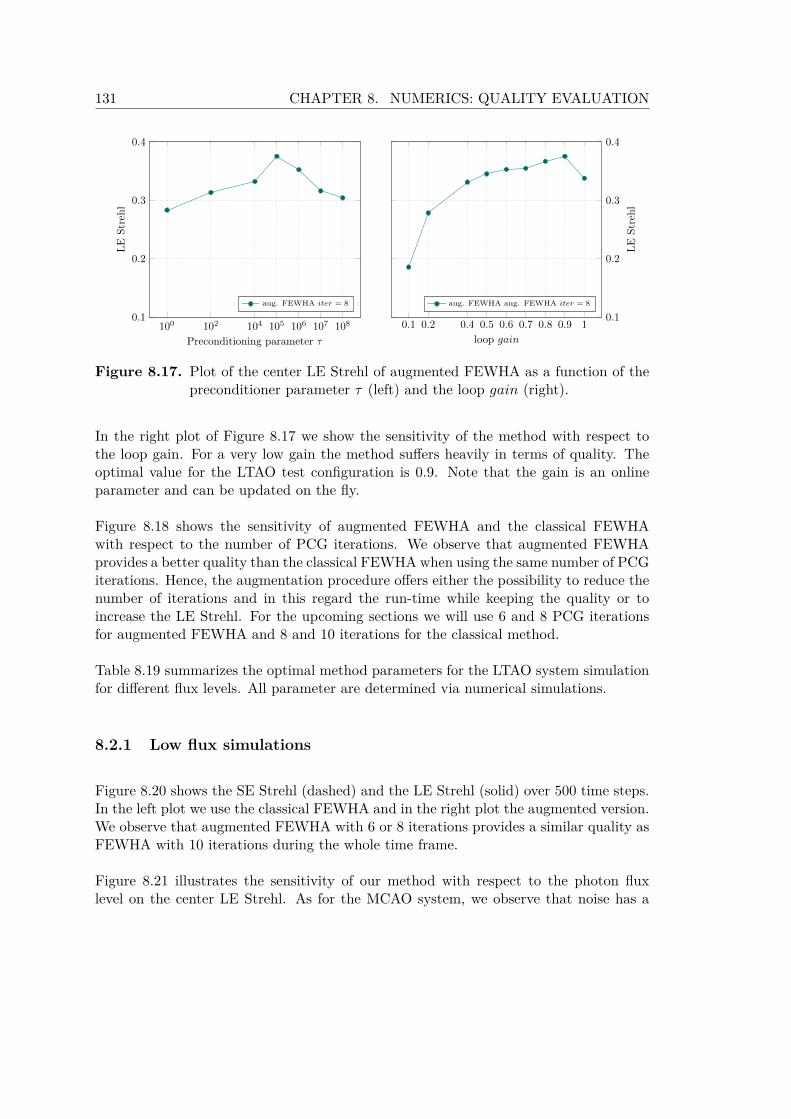
131 CHAPTER 8. NUMERICS: QUALITY EVALUATION
100 102 104 105 106 107 1080.1
0.2
0.3
0.4
Preconditioning parameter τ
LE
Streh
l
aug. FEWHA iter = 8
0.1 0.2 0.4 0.5 0.6 0.7 0.8 0.9 10.1
0.2
0.3
0.4
loop gain
LE
Streh
l
aug. FEWHA aug. FEWHA iter = 8
Figure 8.17. Plot of the center LE Strehl of augmented FEWHA as a function of thepreconditioner parameter τ (left) and the loop gain (right).
In the right plot of Figure 8.17 we show the sensitivity of the method with respect tothe loop gain. For a very low gain the method suffers heavily in terms of quality. Theoptimal value for the LTAO test configuration is 0.9. Note that the gain is an onlineparameter and can be updated on the fly.
Figure 8.18 shows the sensitivity of augmented FEWHA and the classical FEWHAwith respect to the number of PCG iterations. We observe that augmented FEWHAprovides a better quality than the classical FEWHA when using the same number of PCGiterations. Hence, the augmentation procedure offers either the possibility to reduce thenumber of iterations and in this regard the run-time while keeping the quality or toincrease the LE Strehl. For the upcoming sections we will use 6 and 8 PCG iterationsfor augmented FEWHA and 8 and 10 iterations for the classical method.
Table 8.19 summarizes the optimal method parameters for the LTAO system simulationfor different flux levels. All parameter are determined via numerical simulations.
8.2.1 Low flux simulations
Figure 8.20 shows the SE Strehl (dashed) and the LE Strehl (solid) over 500 time steps.In the left plot we use the classical FEWHA and in the right plot the augmented version.We observe that augmented FEWHA with 6 or 8 iterations provides a similar quality asFEWHA with 10 iterations during the whole time frame.
Figure 8.21 illustrates the sensitivity of our method with respect to the photon fluxlevel on the center LE Strehl. As for the MCAO system, we observe that noise has a
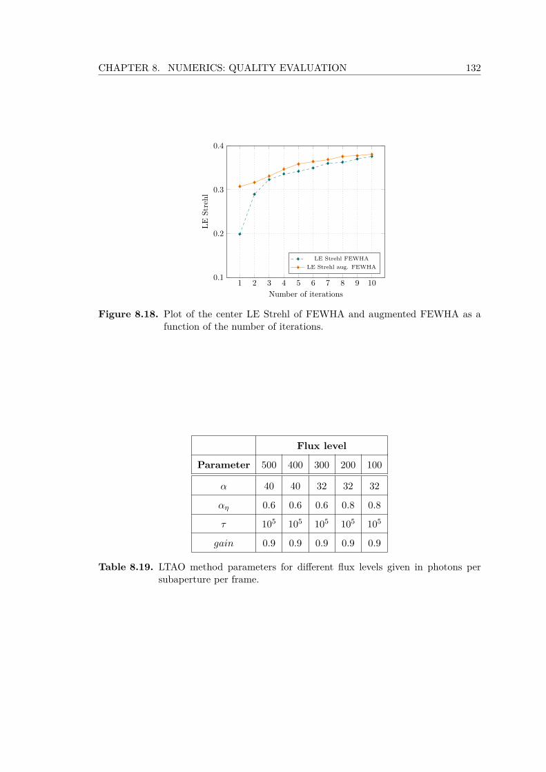
CHAPTER 8. NUMERICS: QUALITY EVALUATION 132
1 2 3 4 5 6 7 8 9 100.1
0.2
0.3
0.4
Number of iterations
LE
Strehl
LE Strehl FEWHA
LE Strehl aug. FEWHA
Figure 8.18. Plot of the center LE Strehl of FEWHA and augmented FEWHA as afunction of the number of iterations.
Flux level
Parameter 500 400 300 200 100
α 40 40 32 32 32
αη 0.6 0.6 0.6 0.8 0.8
τ 105 105 105 105 105
gain 0.9 0.9 0.9 0.9 0.9
Table 8.19. LTAO method parameters for different flux levels given in photons persubaperture per frame.

133 CHAPTER 8. NUMERICS: QUALITY EVALUATION
0 100 200 300 400 5000
0.2
0.4
0.6
Time steps
Streh
lratio
FEWHA
LE Strehl iter = 8
SE Strehl iter = 8
LE Strehl iter = 10
SE Strehl iter = 10
0 100 200 300 400 5000
0.2
0.4
0.6
Time steps
Strehlratio
Augmented FEWHA
LE Strehl iter = 6
SE Strehl iter = 6
LE Strehl iter = 8
SE Strehl iter = 8
Figure 8.20. Plot of the on-axis SE Strehl (dashed) and LE Strehl (solid) over 500time steps. Low flux simulation with nphotons = 500. For FEWHA (left)we use 8 and 10 iterations and for augmented FEWHA (right) 6 and 8iterations.
crucial impact on the performance of augmented FEWHA. With decreasing photon fluxthe method shows deficiencies in the reconstruction quality compared to the classicalmethod when using a smaller number of iterations. Note that if we would increase thenumber of iterations for augmented FEWHA to 8 or 10 the quality becomes at least asgood as for the classical algorithm.
8.2.2 Sensitivity with respect to the Fried parameter
Figure 8.22 shows the on-axis LE Strehl versus the Fried parameter r0 of FEWHA andaugmented FEWHA with PCG iterations as indicated in the legend. Larger valuescorrespond to good seeing conditions, hence, to weak turbulence, whereas smaller valuesrefer to bad seeing and strong perturbations. We observe that the difference betweenaugmented FEWHA with 8 iterations and FEWHA with 10 iterations is negligible.Augmented FEWHA with 6 iterations provides a better quality than FEWHA with 8iterations.
Similar to the MCAO system simulations, the quality evaluation for the LTAO system re-veals that with augmented FEWHA we are able to reduce the number of PCG iterations.We conclude that augmented FEWHA with 6 iterations provides a suitable quality forall simulation performed above. When using augmented FEWHA with 8 PCG iterationswe can increase the reconstruction quality compared to the classical FEWHA. In theupcoming section we focus on the computational performance of augmented FEWHAon real-time hardware architectures.

CHAPTER 8. NUMERICS: QUALITY EVALUATION 134
100 200 300 400 5000
0.2
0.4
0.6
Number of photons/subap./frame
On-axis
LE
Streh
l
FEWHA iter = 8
FEWHA iter = 10
aug. FEWHA iter = 6
aug. FEWHA iter = 8
Figure 8.21. Plot of the on-axis LE Strehl after 500 time steps. Low flux simulationwith photon flux between 100 and 500, spot elongation and a read-outnoise of 3 electrons per subaperture per frame. For FEWHA we use 8 and10 PCG iterations and for augmented FEWHA 6 and 8 PCG iterations.
0.097 0.139 0.157 0.178 0.2340
0.1
0.2
0.3
0.4
0.5
Fried parameter r0
On-axis
LE
Strehl
FEWHA iter = 8
FEWHA iter = 10
aug. FEWHA iter = 6
aug. FEWHA iter = 8
Figure 8.22. Plot of the on-axis LE Strehl of augmented FEWHA with 6 (teal) and8 (orange) iterations versus the Fried parameter r0 after 500 time steps.Low flux simulation with 500 photons per subaperture per frame.

Chapter 9
Numerics: Theoreticalperformance analysis
This section is dedicated to the complexity analysis of the real-time computing (RTC)algorithms. We provide details about the matrix-free representation of the operatorsinvolved and the parallelization possibilities for FEWHA and its augmented version.Moreover, we give a theoretical performance analysis of the MVM algorithm. An esti-mation of the system memory capabilities, necessary to implement the most demandingtasks, is also reported. The analysis treats the hard real-time as well as the soft real-timetasks. We apply the theoretical results to test configurations defined in Chapter 7. Thisenables us to estimate the computational throughput required to decide for a suitablereal-time hardware. The results in this chapter are to a large extent taken from ourpaper about the feasibility of standard and novel solvers for atmospheric tomography in[43].
9.1 Block operators
FEWHA has the ability to represent its components in a matrix-free manner. Sucha representation considerably reduces the required memory as wells as the number ofFLOPs. However, for modern real-time systems the number of FLOPs and memoryusage is not the only performance indicator. Properties such as structured memoryaccesses or parallelization possibilities play a crucial role as well. In the following, wediscuss the matrix-free representation of the block operators of (augmented) FEWHA,such as the SH operator, the bilinear interpolation and the wavelet transform. All ofthem play a significant role in the costs required for the algorithm, i.e., the applicationof M as defined in Equation (5.11). Moreover, these operators are involved in the
135

CHAPTER 9. NUMERICS: THEORETICAL PERFORMANCE ANALYSIS 136
computation of the right-hand side b defined in Equation (5.3.3). In addition, we statethe number of FLOPs and the required memory for the operators. Note that there is nodifference in the discretization between FEWHA and its augmented version, and thus thematrices involved coincide. Hence, the descriptions below are valid for both algorithms.The computational estimates are mainly based on the number of subapertures n2
s of theWFSs in use and the number of layer discretization points nlay = 22Jℓ , where Jℓ denotesthe number of wavelet scales on layer ℓ.
9.1.1 SH operator
For a specific SH WFS with n2s subapertures the operator Γ maps wavefronts to the
average x- and y-slopes of the subapertures of the WFSs. We discretize these wavefrontsby continuous piecewise bilinear functions with (ns + 1)2 nodal values. Hence, thedimension of Γ is 2n2
s × (ns + 1)2. Storing a full matrix of this dimension requires2n2
s(ns + 1)2 units of memory. The number of FLOPs for performing a matrix-vectormultiplication with this matrix sum up to 4n3
s(ns +2). The piecewise bilinear basis usedfor discretization has local support. In fact, it interacts with at most four subapertures.The measurement in a single subaperture is only influenced by the wavefront function atthe corner points of the respective subaperture. Thus, one row of Γ, which correspondsto one subaperture, has only four non zero entries. This sparse matrix representationenables to considerably reduce the FLOPs to 14n2
s and the memory requirements to 8n2s.
The structure of Γ offers the possibility to implement the operator in matrix-free way,which further reduces the FLOPs and memory usage. We split the computation of x-slopes in Equation (2.11) into two parts. In a first step, we calculate and store thedifferences between the nodal values. In a second step, we calculate the averages. Thesame procedure is applied for the y-slopes in Equation (2.12). The total number ofFLOPs for the matrix-free implementation decreases to 6n2
s + 2ns and the memoryusage to n2
s + ns.
9.1.2 Bilinear interpolation
The bilinear interpolation operator Pgℓ maps the reconstructed layers to wavefronts usingpiecewise bilinear basis functions. The layers are discretized using a grid with 2Jℓ × 2Jℓ
points and the wavefronts using a grid with (ns + 1) × (ns + 1) values projected ontolayer ℓ and guide star direction g; see Figure 9.1. The dimension of the full matrixPgℓ is 22Jℓ+1 × (ns + 1)2. Hence, the operation in a full matrix representation requires(22Jℓ+1−1)(ns+1)2 FLOPs and 22Jℓ(ns+1)2 units of memory. However, these quantitiescan be optimized by a matrix-free representation.

137 CHAPTER 9. NUMERICS: THEORETICAL PERFORMANCE ANALYSIS
Figure 9.1. Square grid of layers Ωℓ in black with 22Jℓ = 24 points and equidistantspacing. Projected grid of subapertures Ω in red with n2
s = 16 subaperturesobtained by a bilinear interpolation. The blue rectangles represent theresult after a linear interpolation in x-direction.
A bilinear interpolation is the concatenation of two linear interpolations, one in x- andone in y-direction. We utilize this fact for an efficient matrix-free representation. Weillustrate the procedure on the example of Figure 9.1. In a first step, we interpolate inx-direction and obtain as results the blue rectangles. Afterwards, we interpolate in y-direction and obtain the projected grid (red). A matrix-free linear interpolation requires2(ns + 1) units of memory and 3 operations per interpolation point. Altogether, thisleads to (ns + 1)2 + 4(ns + 1) units of memory and at most 6(ns + 1)2 FLOPs. Thenumber of operations here depends on the guide star direction and the altitude of therespective layer, thus, we state an upper bound.
9.1.3 Wavelet transform
The discrete wavelet transform (DWT) W and its transposed operator W T consist ofthe application of the direct transformation matrices Wj and W T
j , respectively, at eachwavelet scale j = 0, ..., J − 1. These matrices can be represented by a set of convolutionoperations with the corresponding wavelet coefficients. In fact, the representation as aconvolution is more efficient than using sparse matrices; see, e.g. [123].
The wavelet coefficients are stored within a matrix of dimension 2j+1×2j+1. Hence, theoverall costs for applying the direct or inverse DWT with a wavelet filter of length p are
J−1∑j=0
2(2p− 1)22(j+1) = 83(2p− 1)(22J − 1),
where J is the overall number of wavelet coefficients. In all our simulations we useDaubechies 3 wavelets, i.e., p = 6, which leads to (88/3)(22J − 1) FLOPs. In terms of

CHAPTER 9. NUMERICS: THEORETICAL PERFORMANCE ANALYSIS 138
memory we have to store the wavelet filter of length p, which is almost negligible, and atemporary variable for the intermediate results at scale j for the application of Wj andW T
j . Summarizing, this leads to 22J units of memory in the matrix-free implementation.
9.1.4 Inverse covariance of noise
The inverse noise covariance operator C−1η in the direction of an LGS consists of the
correlation information between the measurements x-x, y-y, x-y and y-x. Since thecorrelation between x-y and y-x coincides, the matrix is symmetric. Hence, we onlyneed to store 3 vectors of size n2
s. These vectors only change when the WFS geometryor the laser launch position is changed. We apply this operator by multiplying themeasurement vector by the 3 vectors. For an NGS direction we only have to store thescalar parameter σ−2. To summarize, the operator requires for an LGS direction 6n2
s
FLOPs and for an NGS direction 2n2s FLOPs. The memory consumption sums up to
6n2s for LGSs and essentially 0 for NGSs.
9.1.5 Tip-tilt removal operator
The tip-tilt removal operator (I − T ) calculates the average slopes of the measurementsin x- and y-direction, respectively. These average values correspond to the tip and tiltof the wavefront, and thus are subtracted from the measurements. In total, this leadsto 4n2
s FLOPs and no additional memory consumption.
9.1.6 Inverse covariance of turbulence
Finally, we discuss the operator D, which approximates the inverse covariance matrixof turbulence C−1
ϕ , see Section 6.4.2, with a diagonal matrix. Here we only store theweights at each wavelet scale, which sum up to 22Jℓ FLOPs and a memory consumptionof Jℓ.
9.1.7 Performance estimates
Table 9.2 and Table 9.3 summarize the performance estimates of the matrix-free opera-tors described above in terms of FLOPs and memory usage. In addition to the theoreticalresults, we provide the values for the MAORY test configuration defined in Chapter 7.We observe that both quantities have significantly smaller values when using a matrix-free representation. Especially for the wavelet transform, which is the most demanding

139 CHAPTER 9. NUMERICS: THEORETICAL PERFORMANCE ANALYSIS
operator, the difference is significant. The reduction in the number of FLOPs is of order2 · 103 and for the memory usage of order 16 · 103. A performance optimization for thefull matrix representation by using sparse matrices is possible, but not considered in thisthesis.
Operator Full matrix FLOPs Matrix-free FLOPs
SH matrix 2n2s(ns + 1)2 = 61.605M 6n2
s + 2ns = 33.004k
Bilin. interpolation (22Jℓ+1 − 1)(ns + 1)2 = 184.314M 6(ns + 1)2 = 33.750k
Wavelet transform (22Jℓ+1 − 1)22Jℓ+1 = 1.074G 883 (22Jℓ − 1) = 480.570k
Inv. cov. noise LGS (2n2s − 1)n2
s = 59.968M 6n2s = 32.856k
Inv. cov. noise NGS (2n2s − 1)n2
s = 59.968M 2n2s = 10.952k
TT removal (2n2s − 1)n2
s = 59.968M 4n2s = 21.904k
Inv. cov. turbulence (2 · 22Jℓ − 1)22Jℓ = 536.85M 22Jℓ = 16.384k
Table 9.2. Theoretical FLOPs for the operators of (augmented) FEWHA for thematrix-based as well as the matrix-free version. The values correspondto the MAORY test configuration and indicate the significant benefit of thematrix-free representation.
9.2 Parallelization
Without parallelization it would not be possible to meet the real-time requirements ofa large AO system as, e.g., required for the control of the ELT. The hard- and softreal-time costs for the MVM are mainly caused by computing the pseudo open loopslopes and the deformable mirror commands in hard real-time and the (FR) matrixupdate in soft real-time. All these operations consist of matrix-vector multiplications andcan be efficiently parallelized using standard linear algebra libraries. For (augmented)FEWHA parallelization is more complicated, because of the more complex structureof the algorithm. In fact, the method allows two types of parallelization, which werefer to as global and local parallelization. By global parallelization we understand thedecomposition of the operators involved into L or W blocks. Local parallelization refersto parallelization inside these blocks. The combination of these two strategies leadsto a very efficient parallelization scheme. The parallelization strategy for augmentedFEWHA is the same as for the original algorithm.

CHAPTER 9. NUMERICS: THEORETICAL PERFORMANCE ANALYSIS 140
Operator Full matrix mem. usage Matrix-free mem. usage
SH matrix 2n2s(ns + 1)2 = 61.61MB n2
s + ns = 5.55kB
Bilin. interpolation 22Jℓ(ns + 1)2 = 921.60kB (ns + 1)2 + 4(ns + 1) = 5.93kB
Wavelet transform 24Jℓ = 268.44MB 22Jℓ = 16.38kB
Inv. cov. noise LGS n4s = 29.987MB 6n2
s = 32.86kB
Inv. cov. noise NGS n4s = 29.987MB 0
TT removal n4s = 29.987MB 0
Inv. cov. turbulence 24Jℓ = 268.44MB Jℓ = 7B
Table 9.3. Memory usage in Byte for the operators of (augmented) FEWHA for fullmatrices as well as for the matrix-free version. The values correspond tothe memory usage for the MAORY test configuration and demonstrate thesignificant benefit of the matrix-free representation.
9.2.1 Global parallelization
We illustrate the idea behind the global parallelization strategy of FEWHA on thematrix-free application of the left-hand side matrix M of Equation (5.10). This op-erator is applied once per PCG iteration and is the computationally most demandingpart of the overall algorithm. Similar strategies are used for the right-hand side b ofEquation (4.15). The matrix M consists of several sparse matrices, in particular, adiscrete wavelet transform, a bilinear interpolation and a SH operator. These matriceshave a block diagonal structure, where the number of blocks corresponds to either thenumber of atmospheric layers L or WFSs W . Since this block structure decouples theproblem, we have the possibility to parallelize over either the number of layers L orWFSs W . However, parallelization can not be applied perfectly, because after a certainnumber of steps synchronization is necessary. Figure 9.4 shows a schematic represen-tation of the global parallelization scheme. The kernels indicated on the right side ofthe figure refer to the parallel blocks of the algorithm. Kernel1 performs an inversewavelet transform, which is parallelizable over the number of layers L. Kernel2 appliesthe atmospheric tomography operator A, decomposed into a SH-matrix Γ and a bilinearinterpolation matrix P . Further, the inverse covariance matrix C−1
η is applied togetherwith ΓT . This kernel is parallelized over the number of WFSs W . Finally, Kernel3applies the transposed bilinear interpolation matrix P T , the transposed inverse wavelettransform and adds the regularization term αD in L parallel blocks. After each kernel,FEWHA requires a synchronization step (dashed lines). This is not optimal for certainhardware architectures, especially for GPUs, since they are optimized for computationalthroughput and latency can become a problem.

141 CHAPTER 9. NUMERICS: THEORETICAL PERFORMANCE ANALYSIS
c = (cℓ)Lℓ=1
Layer ℓqℓ = W−1cℓ
Layer 1q1 = W−1c1
Layer LqL = W−1cL
Kernel1
q = (qℓ)Lℓ=1
WFS wφg = Pw1q1
for l = 2, . . . L
φw = φw + Pwlqℓ
...
WFS 1φ1 = P11q1
for l = 2, . . . L
φ1 = φ1 + P1lqℓ
...
WFS WφG = PW1q1
for l = 2, . . . L
φW = φW + PWlqℓ
...
Kernel2
q = (qw)Ww=1
Layer ℓqℓ = PT
1ℓφ1
for w = 2, . . .W
qℓ = qℓ + PTwℓφw
...
Layer 1q1 = PT
11φ1
for w = 2, . . .W
q1 = q1 + PTw1φw
...
Layer LqL = PT
1Lφ1
for w = 2, . . .W
qL = qL + PTwLφw
...
Kernel3
q = (qℓ)Lℓ=1 = Mc
Figure 9.4. Parallelization of the application of the matrix M over W WFSs and Llayers. The dashed lines indicate synchronization steps.
9.2.2 Local parallelization
Each block of the block diagonal matrices of FEWHA consists of operations that areapplied to a grid of values and can be independently computed from each other. Localparallelization is performed inside each parallel kernel of Figure 9.4. The number ofthreads for local parallelization is related to the size of the block in the respective matrix.The dimensions of the matrices correspond to the number of layer discretization pointsnlay = 22Jℓ and the number of subapertures n2
s. These quantities have values up toa few hundred. For the implementation of these parallelization strategies on certainhardware architectures we refer to Chapter 10. In the following, we provide details onthe parallelization of the matrix-free operators described in Section 9.1.
The SH operator Γ consists of two operations executed sequentially for the x- and y-directions. In particular, the operator computes differences followed by an averagingstep; see Equation (2.11) and Equation (2.12). These operations are performed for agrid of 2(ns + 1)ns values. The computation for each grid point is independent from theother points, and thus can be fully parallelized.

CHAPTER 9. NUMERICS: THEORETICAL PERFORMANCE ANALYSIS 142
The bilinear interpolation consists of two sequential operations. A linear interpolationinto the x-direction and a linear interpolation into the y-direction. Again, the compu-tation is performed on a grid of values, where the computation on each grid point isindependent from the others. Hence, the interpolation into the x- and y-directions canbe parallelized over (ns + 1)2 grid points.
The discrete wavelet transform consists also of two sequential operations at each waveletscale j = 0, . . . , J−1. The direct transform sequentially applies the operator Wj twice tomatrices of dimension 2j+1×2j+1. The inverse transform applies the same operation, butwith the matrix W T
j ; see Equation (4.26). Each of the (2j+1)2 entries of the resultingmatrices can be calculated independently from the others. Hence, parallelization isapplied over (2j+1)2 entries.
Note that the parallelization over all grid points is just a theoretical outcome. In prac-tice, one is limited by the amount of threads that are available on a certain hardwarearchitecture. Moreover, depending on the hardware it can be more efficient to split thework to a smaller number of threads.
9.3 Overall hard and soft real-time FLOPs
In this section, we present the theoretical performance estimates of FEWHA, augmentedFEWHA and the MVM algorithm in terms of FLOPs. We distinguish between FLOPsthat are required to perform the hard real-time task and those required for soft real-time.
9.3.1 Wavelet reconstructor
The most time consuming steps for the hard real-time of (augmented) FEWHA are theapplication of M in the atmospheric tomography step and partially in computing theright-hand side and the fitting step. Below, we provide the number of FLOPs requiredfor all the components within the augmented FEWHA algorithm.
Based on the estimates for the block operators in Section 9.1 we are able to analyzethe computational cost for each component of our algorithm. For the sake of simplicitywe make the following assumptions: The WFSs associated to all the guide stars use thesame geometry with n2
s subapertures. Moreover, we assume that all layers are discretizedusing the same number of points. Note that there is a linear relation between the numberof layer discretization points and the number of subapertures. The number of waveletscales J is chosen in a way that the grid of layers overlaps the wavefront grid, i.e.,
22(Jℓ−1) < (ns + 1)2 ≤ 22Jℓ .

143 CHAPTER 9. NUMERICS: THEORETICAL PERFORMANCE ANALYSIS
Let us neglect the preconditioner and the left-hand side operator for a moment. Thenthe PCG method, as shown in Algorithm 2, consists of 8 vector operations. The diagonalJacobi preconditioner is stored in a single vector of size 22JL. Hence, the applicationof the preconditioner requires 22JL FLOPs. In total, one iteration of the PCG methodrequires 9 · 22JL FLOPs plus the FLOPs for applying the left-hand side operator. Theparameter J denotes the number of wavelet scales on all layers ℓ = 1, . . . L. We can applyparallelization within the PCG method in terms of vector operations. For the augmentedPCG there are two additional parts: the projection of the initial guess c0 and the initialresidual r0 onto the Krylov subspace of the previous system and the projection of thedescent directions pk onto the last vector of the descent directions of the previous systempm in every time step. Our numerical simulations in Chapter 8 reveal that we are ableto significantly reduce the number of PCG iterations with the augmentation procedure.Hence, the overhead induced for augmented FEWHA should be easily compensated bythe reduction in the number of iterations.
In the mirror fitting step we apply two subsequent operations. First, the reconstructedlayers are transformed back from the wavelet domain into the bilinear domain. After-wards, the fitting operation is applied depending on the AO system; see Section 6.5. Inthis thesis we focus on a 3 layer MCAO and a 9 layer LTAO system. For the 3 layerMCAO system we do not need any fitting step, since the layers are directly reconstructedat the altitudes of the DMs. Hence, only the wavelet transform at every layer remains,which requires 88
3 L(22J−1) FLOPs. Note that this operation can be performed in paral-lel over the number of layers L. For the LTAO system we have an additional projectionstep, which requires 7(L− 1)n2
a FLOPs.
Table 9.5 shows the overall FLOPs for FEWHA and its augmented version. The addi-tional FLOPs for augmented FEWHA are marked in orange. The term 9n2
layL · naugIter
is related to the projection of the initial residual, whereas the term 4n2layL corresponds
to the projection in each iteration. Instead of niter only naugIter iterations are performed.
Next, we determine the number of FLOPs of the direct MVM method.
9.3.2 MVM method
The main contribution in terms of computational costs for the soft real-time part of theMVM is the update of the (FR) matrix and there, in particular, the matrix inversion.The computational costs listed in Table 9.6 are estimated assuming that the matrixinversion is performed through a Cholesky decomposition. Note that one benefit of(augmented) FEWHA is that there are no additional soft real-time costs. Because it isan iterative approach, there is no need to precompute any inverse matrix and the wholecomputation is done in hard real-time. The hard real-time computational costs for the

CHAPTER 9. NUMERICS: THEORETICAL PERFORMANCE ANALYSIS 144
Computation step FLOPs
POL data computation (8n2s + 2ns)G
Right hand side [14GLGS + 2GNGS + 6G]n2s + 2Gns
+[(L− 1)(8.5GLGS + 10GNGS) + L(G− 1)](ns + 1)2
+(L+ 1) + 883 (4n2
lay − 1) + n2layL
Update residual 2n2layL
PCG method [14GLGS + 2GNGS + 12G]n2s + 4Gns
FEWHA +[(L− 1)(15.6GLGS + 18GNGS) + L(G− 1)](ns + 1)2
+L1763 (4n2
lay − 1) + 13n2layLniter
PCG method [14GLGS + 2GNGS + 12G]n2s + 4Gns
aug. FEWHA +[(L− 1)(15.6GLGS + 18GNGS + L(G− 1)](ns + 1)2
+L1763 (4n2
lay−1)+13n2layL+(9n2
layL+ 4n2layL)naugIter
Fitting (L− 1)M(ns + 1)2 + L883 (4n2
lay − 1) + Ln2lay
Control 3n2a
Table 9.5. Hard real-time FLOPs for FEWHA and its augmented version. The ad-ditional FLOPs for augmented FEWHA and the different number of PCGiterations are marked in orange.
MVM are dominated by two contributions, which require about the same amount ofoperations: the pseudo open loop (POL) slopes computation, similar to (augmented)FEWHA, and the computation of the deformable mirror commands via a matrix-vectormultiplication. The results are summarized in Table 9.7. The parameter nopt denotesthe number of optimization directions and nml is the number of modes used in the modaldescription of each layer.
9.3.3 Overall FLOPs for the MCAO configuration
In order to compare the computational throughput required for the MVM, FEWHA andaugmented FEWHA, we apply the theoretical results from above to the MAORY testconfiguration defined in Chapter 7. The MCAO system is considerably complex andprovides a suitable example to illustrate the advantages of (augmented) FEWHA.
The left plot of Figure 9.8 shows the hard and soft real-time FLOPs for the MVM (red),

145 CHAPTER 9. NUMERICS: THEORETICAL PERFORMANCE ANALYSIS
Computation step FLOPs
Computation of R n6s + 4nmln
4sL+ (2n2
mlL− nmlL+ 2)n2s
Computation of F n3a + (2nml + 2nmlL+ nopt − 1)n2
s
+(2n2mlL+ n2
optnmlL− 3nmlL)na
Computation of FR (2nmlL− 1)n2an
2s
Table 9.6. Soft real-time FLOPs for the MVM algorithm.
Computation step FLOPs
POL data computation 2n2sGn
2a − n2
sG+ 6nsG
Matrix vector mult. (FR)s 2n2an
2sG− n2
a
Table 9.7. Hard real-time FLOPs for the MVM algorithms.
FEWHA (teal) and augmented FEWHA (orange). We observe the benefits of FEWHAand its augmented version compared to the MVM. Both wavelet reconstructors requireonly about 1/12 of the hard real-time FLOPs compared to the MVM. For the soft real-time part, since (augmented) FEWHA does not involve any significant computation,there is an evident advantage compared to the MVM algorithm.
HRT SRT
0
0.5
1
1.5
2
2.5
TFL
OPs
MVMFEWHA
aug. FEWHA
HRT SRT
0
0.5
1
1.5
2
2.5
TFL
OPs
MVMFEWHA
aug. FEWHA
Figure 9.8. Hard and soft real-time FLOPs for one time step for the MVM algorithm(red), FEWHA (teal) and augmented FEWHA (orange). In the left plotwe simulate the MCAO system and in the right plot the LTAO system.
We assume naugIter = niter/2, i.e., 4 iterations for FEWHA and 2 for augmented FE-WHA. Then the classical PCG method used within FEWHA requires 63.5 MFLOPs andthe augmented PCG 33.5 MFLOPs. This results in a reduction of about 20% of FLOPs
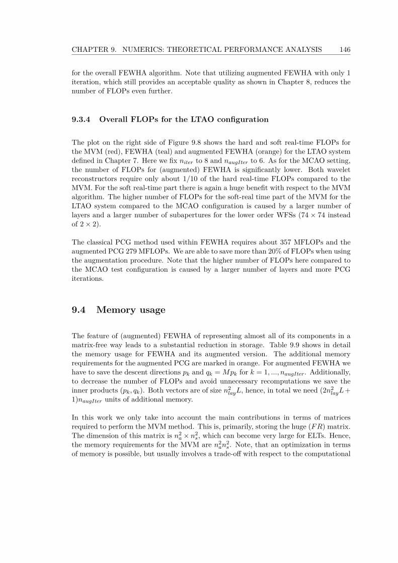
CHAPTER 9. NUMERICS: THEORETICAL PERFORMANCE ANALYSIS 146
for the overall FEWHA algorithm. Note that utilizing augmented FEWHA with only 1iteration, which still provides an acceptable quality as shown in Chapter 8, reduces thenumber of FLOPs even further.
9.3.4 Overall FLOPs for the LTAO configuration
The plot on the right side of Figure 9.8 shows the hard and soft real-time FLOPs forthe MVM (red), FEWHA (teal) and augmented FEWHA (orange) for the LTAO systemdefined in Chapter 7. Here we fix niter to 8 and naugIter to 6. As for the MCAO setting,the number of FLOPs for (augmented) FEWHA is significantly lower. Both waveletreconstructors require only about 1/10 of the hard real-time FLOPs compared to theMVM. For the soft real-time part there is again a huge benefit with respect to the MVMalgorithm. The higher number of FLOPs for the soft-real time part of the MVM for theLTAO system compared to the MCAO configuration is caused by a larger number oflayers and a larger number of subapertures for the lower order WFSs (74 × 74 insteadof 2× 2).
The classical PCG method used within FEWHA requires about 357 MFLOPs and theaugmented PCG 279 MFLOPs. We are able to save more than 20% of FLOPs when usingthe augmentation procedure. Note that the higher number of FLOPs here compared tothe MCAO test configuration is caused by a larger number of layers and more PCGiterations.
9.4 Memory usage
The feature of (augmented) FEWHA of representing almost all of its components in amatrix-free way leads to a substantial reduction in storage. Table 9.9 shows in detailthe memory usage for FEWHA and its augmented version. The additional memoryrequirements for the augmented PCG are marked in orange. For augmented FEWHA wehave to save the descent directions pk and qk = Mpk for k = 1, ..., naugIter. Additionally,to decrease the number of FLOPs and avoid unnecessary recomputations we save theinner products (pk, qk). Both vectors are of size n2
layL, hence, in total we need (2n2layL+
1)naugIter units of additional memory.
In this work we only take into account the main contributions in terms of matricesrequired to perform the MVM method. This is, primarily, storing the huge (FR) matrix.The dimension of this matrix is n2
a × n2s, which can become very large for ELTs. Hence,
the memory requirements for the MVM are n2an
2s. Note, that an optimization in terms
of memory is possible, but usually involves a trade-off with respect to the computational

147 CHAPTER 9. NUMERICS: THEORETICAL PERFORMANCE ANALYSIS
Computation step Memory usage
POL data computation (2n2s + nsnphi)G
Right hand side G+ [0.7GLGS +GNGS ](L− 1)(ns + 1)2 + Ln2lay
Update residual L22Jl
PCG method 2Gn2s +G+ [0.7GLGS +GNGS ](L− 1)(ns + 1)2
FEWHA +Gnsnphi + 4Ln2lay
PCG method 2Gn2s +G+ [0.7GLGS +GNGS ](L− 1)(ns + 1)2
aug. FEWHA +Gnsnphi + 4Ln2lay + (2n2
layL+ 1)naugIter
Fitting G(L− 1)(ns + 1)2 + 2Ln2lay
Control Mn2a
Table 9.9. Required memory for FEWHA and the additional memory consumption foraugmented FEWHA (orange).
time. Here, we do not consider any optimization strategies.
9.4.1 Memory usage for the MCAO configuration
We illustrate the benefits of FEWHA and its augmented version in terms of memoryusage on the test case of MAORY. The left plot of Figure 9.10 shows the units ofmemory in GB required for the MVM (red), FEWHA (teal) and augmented FEWHA(orange). Note that we assume here single precision (32 bit) floating point numbers. Weobserve the significant lower memory requirement of FEWHA (8 MB) and its augmentedversion (8.8 MB) compared to the MVM algorithm. The memory intensive MVM methodrequires 53 GB, mainly caused by storing the huge (FR) matrix.
The additional units of memory required for the augmentation procedure sum up toapproximately 0.8 MB for this test configuration. Compared to the overall memoryusage of FEWHA and especially compared to the memory intensive MVM method thisadditional units of memory are almost negligible.

CHAPTER 9. NUMERICS: THEORETICAL PERFORMANCE ANALYSIS 148
Memory usage
0
20
40
60G
Byte
MVMFEWHA
aug. FEWHA
Memory usage
0
20
40
60
GBy
te
MVMFEWHA
aug. FEWHA
Figure 9.10. Memory usage for the MVM (red), FEWHA (teal) and augmented FE-WHA (orange) for the MCAO (left) and LTAO (right) configuration.
9.4.2 Memory for the LTAO configuration
In the plot on the right side of Figure 9.10 we illustrate the amount of memory inGB required for the MVM (red), FEWHA (teal) and augmented FEWHA (orange) forthe LTAO system configuration. We observe a significant lower memory requirementfor FEWHA (15 MB) and its augmented version (20.6 MB) compared to the MVMalgorithm (60 GB).
The additional storage costs for the augmentation procedure sum up to 5.6 MB for thistest configuration. Again we conclude that compared to the overall memory usage thesecontributions are almost negligible.
9.5 Real-time system
We determine a possible real-time hardware architecture, on the basis of the computa-tional throughput requirements ascertained in the previous sections. We base the archi-tectural design on the results accumulated within the GreenFlash research activity; see[38, 39]. The outcome of this study, in which CPU, FPGA and GPU technologies havebeen compared, has indicated that the most suitable technology for the computationalengine of an ELT-class real-time hardware system is the GPU. Another important out-come of the study is that the FPGA technology is still superior for the smart-interfacing,i.e., at providing the interfaces between sensors and mirrors and the computational core.However, the Greenflash studied assumed the MVM as a reconstruction algorithm anddid not consider (augmented) FEWHA.

149 CHAPTER 9. NUMERICS: THEORETICAL PERFORMANCE ANALYSIS
Taking into account the computational load determined for the MVM, a single GPUwould not achieve the computational throughput needed to meet the real-time require-ments of MAORY. Thus, we suggest to use an off-the-shelf product, namely, the DGX-1supercomputer by NVIDIA; see [124]. This workstation is equipped with 8 Tesla V100GPUs connected by a dedicated ultra high speed bus (NVLINK). We suggest to use theDGX-1 for the hard as well as the soft real-time engine. Since the computational loadof FEWHA is significantly lower, in theory, a single Tesla V100 or an off-the-shelf CPUshould provide enough computational power to meet the real-time requirements. More-over, for FEWHA no additional soft real-time engine is needed. Altogether, this leadsto significant lower hardware requirements and likewise costs for (augmented) FEWHAcompared to the MVM.


Chapter 10
Numerics: Performance onreal-time hardware
This chapter is dedicated to a detailed study on the computational performance ofFEWHA and augmented FEWHA on different real-time hardware architectures. Thecontrol of a large AO system, required for the new generation of ELTs, is a complexand crucial task. In order to meet the real-time requirements, an efficient reconstructorimplemented on a high performance hardware architecture is inevitable. We focus hereon the implementation of FEWHA and its augmented version on CPU and GPU, basedon our analysis in Section 9.5. We provide an overview on several parallel programmingmodels for CPUs and GPUs, which we utilize for performance optimization. We followthe work in [40] for CPUs and [41] for GPUs. The run-time analysis for FEWHA andits augmented version on CPU and GPU is performed for the test configurations definedin Chapter 7. The results presented in this chapter are mainly based on our work aboutthe parallel implementation of an iterative solver for atmospheric tomography in [26].
10.1 Implementation on CPU
In the following, we describe two concepts for parallelization on a multi-core CPU,namely, threads and vectorization. We use both of them for the parallelization of FE-WHA and augmented FEWHA. The first one is employed for the global parallelizationscheme, whereas the second one is used for local parallelization of the individual op-erators; see Section 9.2. The global parallelization strategy on CPUs is implementedthrough the popular environment OpenMP1, which is a portable standard for shared
1https://www.openmp.org/
151

CHAPTER 10. NUMERICS: PERFORMANCE ON REAL-TIME HARDWARE 152
memory programming. OpenMP is supported by several compilers like, e.g., GCC orClang. For local parallelization we apply the concept of vectorization using Intel AVX22
vector instructions.
10.1.1 Thread programming
We implemented the global parallelization scheme of (augmented) FEWHA on the CPUusing OpenMP, which turned out to be very efficient for parallelizing simple loops indifferent applications as shown, e.g., in [125–127]. Each kernel in Figure 9.4 correspondsto a parallel OpenMP region. In addition to the omp parallel for directive, whichindicates a parallelizable loop, we use the variable OMP_NUM_THREADS to restrictthe regions to either L or W threads. For more details on OpenMP we refer to Chapter 3.
10.1.2 Single Instruction Multiple Data
For CPUs it has been shown, e.g. in [128], that for problems involving task and dataparallelization techniques, Single Instruction Multiple Data (SIMD) vectorization is acrucial concept for achieving reasonable performance. This is in agreement with whatwe observe for FEWHA and its augmented version. During our studies it turned outthat the combination of OpenMP parallel regions for global parallelization and vectorextensions for local parallelization provides best results. In contrast, using OpenMPnested parallelism induces too much overhead. This is reported for other applicationsas well, e.g., in [129]. Several loops inside the FEWHA algorithm are already auto-vectorized by the GCC compiler. However, when dealing with more complex constructs,compilers come to their limits; see, e.g., [130]. That is why we add explicit vectorizationfor the discrete wavelet transform, the SH operator and the bilinear interpolation to fullyexploit the computational potential of the CPU. Since version 4.0 OpenMP supportsSIMD instructions by using the directive omp simd. This statement indicates that therespective loop can be transformed into a SIMD loop. Beside OpenMP, there existseveral other ways to include explicit SIMD vectorization. In fact, in all our simulationsIntel intrinsics provide best results.
10.2 Implementation on GPU
On the NVIDIA Tesla V100 GPU; see Section 7.3 for the hardware specifications; weutilize CUDA 10.1 to implement the parallelization scheme. CUDA offers special C++
2https://software.intel.com/content/www/us/en/develop/documentation/cpp-compiler-developer-guide-and-reference/top/compiler-reference/intrinsics.html

153 CHAPTER 10. NUMERICS: PERFORMANCE ON REAL-TIME HARDWARE
functions, called kernels, that are executed in parallel by a certain number of threads.For more details on CUDA we refer to Chapter 3.
In a first attempt, we utilized unified memory for the parallel version on the GPU.This concept handles the copy operations between CPU and GPU automatically, andthus provides an easy way to port an existing C++ code to CUDA. However, numericalsimulations show that this approach is not satisfying and we decided to handle these copyoperations by our own. In fact, for the final implementation of FEWHA and augmentedFEWHA all computations are done by the GPU. This strategy minimizes host/devicememory transfers, which are costly in terms of computational performance. We utilizeCUDA kernels with L or W blocks for global parallelization. Although, L and W areusually low (below 10) the global parallelization strategy provides a significant speed upof the overall method, since the computations inside are very time intensive.
CPU GPU CPU GPU
Without dynamic parallelism With dynamic parallelism
Figure 10.1. Concept of dynamic parallelism.
The local parallelization scheme on the GPU is implemented using CUDA dynamicparallelism with an optimized number of threads; see Figure 10.1. This concept makesit possible to launch kernels from threads, which run on the device, i.e., a thread canlaunch other threads. We implement the discrete wavelet transform similar to the oneproposed in [131] and [132]. Moreover, we apply various optimization techniques thatare common for NVIDIA GPUs. Global memory loads and stores of the 32 threads of awarp are merged by NVIDIA GPUs into the fewest possible number of transactions. Thiseffect is known as memory coalescing. We utilize this feature and align the data for theoperators to minimize the DRAM bandwidth usage. In addition, CUDA provides userdefined vectorized memory load and store instructions, similar to the SIMD instructionswe used for local parallelization on the CPU. Utilizing these vectorization strategy it waspossible to improve the performance of the operators even further. These operations loadand store data in 64- or 128-bit widths, and thus reduce the total number of instructions

CHAPTER 10. NUMERICS: PERFORMANCE ON REAL-TIME HARDWARE 154
and latency, and improve bandwidth utilization. The fact that global memory and sharedmemory have different speed in access by several orders of magnitude offers anotherpossibility to improve performance. Because shared memory is on-chip, the latency isroughly 100 times lower than for uncached global memory on a NVIDIA Tesla V100GPU; see [124]. We utilize shared memory for the implementation of the matrix-free SHoperator. This operator reuses data elements from memory, thus, moving these elementsfirst to shared memory and being able to access them afterwards with lower latency isbeneficial for the computational performance. Unfortunately, the other operators do notshare this structure and shared memory does not yield comparable gains.
10.2.1 Optimized implementation of the PCG method
Based on the work in [133] we use an optimized version of the PCG for GPUs, whichis shown in Algorithm 7. Our aim is to minimize the number of kernel calls, globalmemory loads and the communication overhead. By (·, ·) we denote the standard ℓ2scalar product. These scalar products are grouped together and computed within asingle kernel to reduce the number of synchronizing steps and kernels on GPU and CPU(steps 6-7). Within the main loop we load vectors at the same place and apply vectoroperations within a single kernel to allow multiple operations to reuse the data (steps9-12). In the end, this approach has more floating point operations than the originalone, however, shows a better performance on the GPU.
10.3 Computational performance for different AO systems
This section is dedicated to a detailed study of the computational performance of aug-mented FEWHA for different AO systems on a multi-core CPU and a GPU. We startwith analyzing the local parallelization strategy, which is valid for both methods andall test configurations listed in Chapter 7. We continue with the overall run-time of thealgorithms for the LTAO and MCAO system configuration defined in Chapter 7.
10.3.1 Performance of the local parallelization strategy
The performance verification for the local parallelization strategy of augmented FEWHAinvolves the run-time analysis of the matrix-free block operators, i.e., the bilinear inter-polation, the SH operator and the discrete wavelet transform as described in Section 9.1.Figure 10.2 shows the block operators on the CPU (red) and on the GPU (green). Notethat there is no difference between FEWHA and its augmented version in the localparallelization strategy. Hence, the graphs are valid for both algorithms. Although all

155 CHAPTER 10. NUMERICS: PERFORMANCE ON REAL-TIME HARDWARE
Algorithm 7 PCG on GPU for Mc = b
1: Input: r (residual vector)J (Jacobi preconditioner)M (FEWHA left-hand side operator)c (wavelet coefficient vector)maxIter (max. number of PCG iterations)
2: Output: c (new wavelet coefficient vector), r (new residual vector)3: for iter = 0, 1, ...,maxIter do4: z = J−1r5: s = Mz
6: ρ = (r, z)7: µ = (s, z)8: β = ρ/ρold
9: α = ρ/(µ− ρβ/α)10: ρold = ρ
11: p = z + βp12: q = s+ βq13: c = c+ αp14: r = r − αq15: end for
these operators are applied in a matrix-free manner, the dimensions of the matrices stillinfluence the computational speed. For all simulations we run 1000 loop iterations andtake the average run-time.
In the upper left plot of Figure 10.2 we study the scalability of the discrete wavelettransform W of dimension n2
lay ×n2lay with respect to the number of layer discretization
points nlay. For our test configurations this parameter has a value of 128. We observethat for small matrix sizes the CPU clearly outperforms the GPU version. However,for bigger matrix dimensions the GPU shows its benefits. The time required for theexecution on the GPU grows almost linearly with the matrix sizes. The reason is thatparallelization on GPUs is very efficient. Note that for a higher value of nlay the localparallelization strategy on the CPU, implemented through vectorization, might not beoptimal. However, the optimization for large values of nlay with, e.g., OpenMP nestedparallelism, are beyond the scope of this thesis, since they are not relevant for the testconfigurations defined in Chapter 7.
The upper right plot of Figure 10.2 shows the scalability of the bilinear interpolationoperator P of size (ns +1)2×n2
lay with respect to the number of subapertures ns. We fixnlay to 128 for these test runs. Since the number of entries per row of P is constant; seeSection 9.1; nlay does not influence the overall performance. The number of subapertures
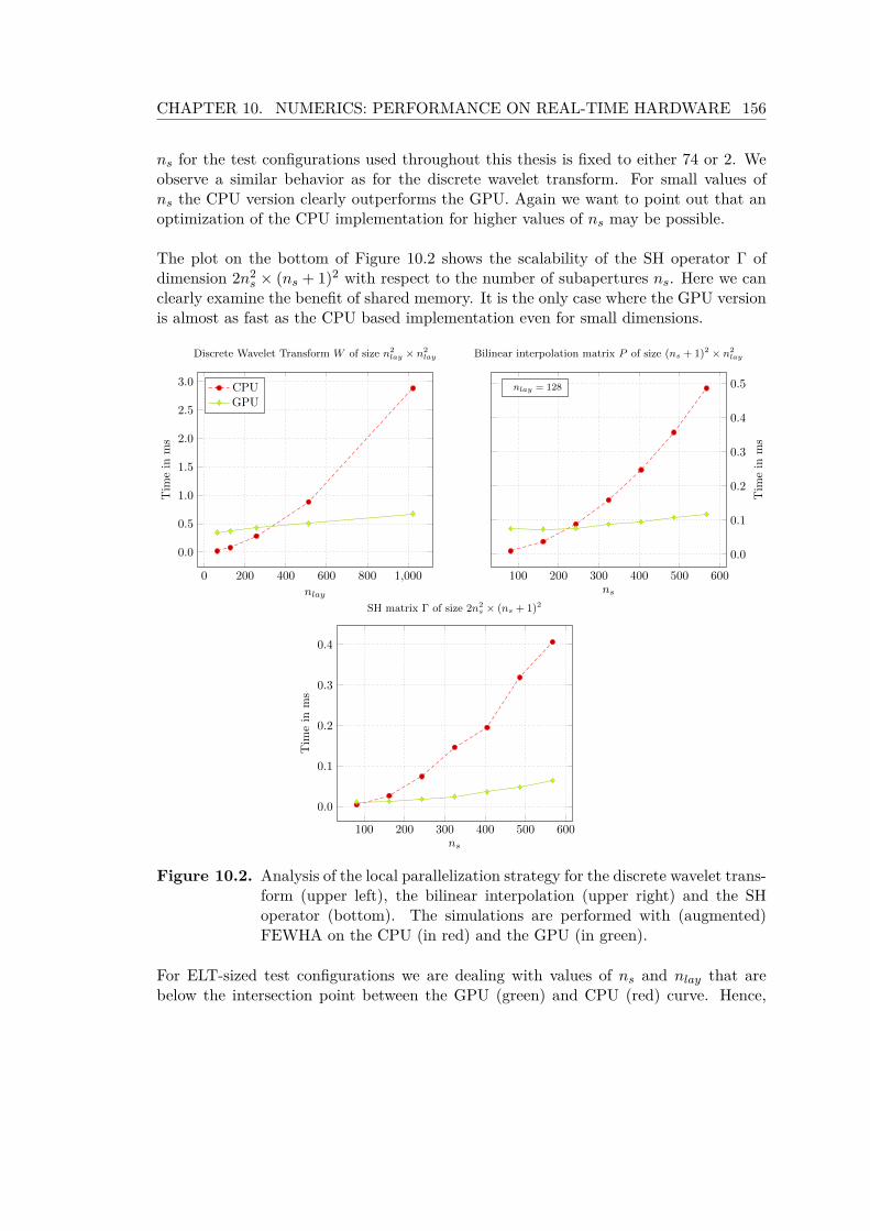
CHAPTER 10. NUMERICS: PERFORMANCE ON REAL-TIME HARDWARE 156
ns for the test configurations used throughout this thesis is fixed to either 74 or 2. Weobserve a similar behavior as for the discrete wavelet transform. For small values ofns the CPU version clearly outperforms the GPU. Again we want to point out that anoptimization of the CPU implementation for higher values of ns may be possible.
The plot on the bottom of Figure 10.2 shows the scalability of the SH operator Γ ofdimension 2n2
s × (ns + 1)2 with respect to the number of subapertures ns. Here we canclearly examine the benefit of shared memory. It is the only case where the GPU versionis almost as fast as the CPU based implementation even for small dimensions.
0 200 400 600 800 1,000
0.0
0.5
1.0
1.5
2.0
2.5
3.0
nlay
Tim
ein
ms
Discrete Wavelet Transform W of size n2lay × n2
lay
CPUGPU
100 200 300 400 500 600
0.0
0.1
0.2
0.3
0.4
0.5
ns
Tim
ein
ms
Bilinear interpolation matrix P of size (ns + 1)2 × n2lay
100 200 300 400 500 600
0.0
0.1
0.2
0.3
0.4
ns
Tim
ein
ms
SH matrix Γ of size 2n2s × (ns + 1)2
nlay = 128
Figure 10.2. Analysis of the local parallelization strategy for the discrete wavelet trans-form (upper left), the bilinear interpolation (upper right) and the SHoperator (bottom). The simulations are performed with (augmented)FEWHA on the CPU (in red) and the GPU (in green).
For ELT-sized test configurations we are dealing with values of ns and nlay that arebelow the intersection point between the GPU (green) and CPU (red) curve. Hence,

157 CHAPTER 10. NUMERICS: PERFORMANCE ON REAL-TIME HARDWARE
for our test configurations the CPU based implementation clearly outperforms the GPUversion for all the matrix-free block operators. Only for larger matrix sizes the GPUstarts to show its benefits. However, these large values are far beyond the scope of theELT specifications and just of academic interest. GPUs outperforming CPUs only foran increasing workload was observed for other applications as well; see, e.g., [134]. Notethat this outcome does not contradict with the GreenFlash study in [38], since theyanalyzed feasible real-time architectures for the MVM method. The MVM approachinvolves considerably more FLOPs; see Section 9.3.3.
10.3.2 Overall performance for the MCAO system simulation
In the following, we provide the run-time results of FEWHA and its augmented versionfor the MAORY test configuration defined in Chapter 7. As hardware we use again onenode of Radon1 for the CPU implementation and a Tesla V100 GPU; see Section 7.3.The main goal of this section is to verify that augmented FEWHA is able to fulfill therun-time requirements of MAORY. To prove this, we use a 3 layer MCAO configurationwith 1 or 2 augmented PCG iterations. In Chapter 8 we verified that this configurationis able to provide a suitable reconstruction quality in terms of LE Strehl ratio. MAORYis operating at 500 Hz, hence, the real-time requirement is 2 ms.
From the left plot of Figure 10.3 we observe the computational performance of FEWHA(teal) and augmented FEWHA (orange) on the multi-core CPU with a varying numberof threads for global parallelization. For augmented FEWHA we use 1 and 2 iterations,whereas for FEWHA we utilize 4 PCG iterations. We observe that we already obtain agood performance with only 3 threads, related to the 3 layers. In fact, the best resultis obtained when using 6 threads. The number 6 here corresponds to the number ofhigh-order WFSs, which have a larger number of subapertures of 74× 74, and thus alsosignificant more computations involved than the 3 low-order ones with 2×2 subapertures.For more than 6 threads the elapsed time stays the same or slightly increases. ComparingFEWHA and its augmented version we observe that augmented FEWHA is faster, causedby the lower number of PCG iterations.
Figure 10.4 shows the performance of FEWHA (teal) and augmented FEWHA (orange)with a different number of PCG iterations on the GPU (left) and the CPU (right). Wereconstruct 3 layers using 3 DMs for wavefront correction as defined in Chapter 7. Weobserve the linear increase in run-time with an increasing number of PCG iterations.This is what we expect as the PCG iterations are not parallelizable. Moreover, we seethat the performance of augmented FEWHA is slightly worse compared to FEWHAwhen using the same number of PCG iterations. This behavior is caused by additionalcomputations involved for the augmentation procedure, such as scalar products andvector updates. Comparing the GPU and the CPU performance we observe that theCPU implementation clearly outperforms the GPU one. On the multi-core CPU we are

CHAPTER 10. NUMERICS: PERFORMANCE ON REAL-TIME HARDWARE 158
1 2 3 4 5 6 7 8 9
1
2
3
4
5
6
7
8
#Threads
Tim
ein
ms
MCAO system
FEWHA iter = 4
aug. FEWHA iter = 1
aug. FEWHA iter = 2
0 1 2 3 4 5 6 7 8 9 10 11 12 130
5
10
15
20
25
30
35
40
45
50
55
#Threads
Tim
ein
ms
LTAO system
FEWHA iter = 8
aug. FEWHA iter = 6
aug. FEWHA iter = 8
Figure 10.3. Scalability of FEWHA and augmented FEWHA with different numberof threads on the CPU for the MCAO configuration (left) and the LTAOsystem (right).
able to fulfill the real-time requirements of 2 ms with augmented FEWHA when using 2 orless PCG iterations. On the GPU the computational performance is far beyond the goal.When using 2 PCG iterations on the CPU the run-time limit is only barely undercut withabout 1.8 ms. However, we have shown in Chapter 8 that the augmentation approachenables to decrease the number of iterations even to 1. Hence, it offers the possibilityto perform the reconstruction in about 1.3 ms with acceptable sacrifices in terms of LEStrehl. If we consider the classical FEWHA with 4 PCG iterations, we are not ableto run the MAORY configuration in real-time. Note that this outcome depends highlyon the CPU in use. An optimization in terms of CPU hardware, e.g., a higher clockfrequency, is possible and would improve the run-time.
Figure 10.5 illustrates the influence of the number of layers in the computational perfor-mance of (augmented) FEWHA. The different number of PCG iterations are indicatedin the legend. The number of DMs is fixed here to the number of layers, in order toomit the mirror fitting step. The first three DMs are configured as listed in Chapter 7,whereas for the additional DMs we use the setting of DM2 in Table 7.6 with altitudesequal to the layer heights. We observe that both algorithms parallelize very well withrespect to the number of layers on the GPU as well as on the CPU. For an increasingnumber of layers, the elapsed time only slightly increases. Moreover, we examine againthat the CPU is considerably faster then the GPU.
We conclude that augmented FEWHA for the MAORY test configuration with 3 layersand 2 PCG iterations is able to meet the real-time requirements on an off-the-shelfCPU, as shown in Figure 10.4. The classical FEWHA with 4 PCG iterations is notable to fulfill this requirement. The poor performance of the GPU compared to the

159 CHAPTER 10. NUMERICS: PERFORMANCE ON REAL-TIME HARDWARE
1 2 3 4 5 6 7 80
2
4
6
8
10
12
14
16
18
#PCG iterations
Tim
ein
ms
Run-time on GPU
FEWHA
aug. FEWHA
1 2 3 4 5 6 7 80
1
2
3
4
5
6
#PCG iterations
Tim
ein
ms
Run-time on CPU
FEWHA
aug. FEWHA
Figure 10.4. Scalability of FEWHA (teal) and augmented FEWHA (orange) with dif-ferent number of PCG iterations on the GPU (left) and CPU (right) forthe MCAO system configuration.
CPU of all our test runs is mainly caused by the following reasons: For the globalparallelization scheme we are just parallelizing over up to 9 layers, or 9 WFSs, which isfar too little to fully exploit GPU resources. This outcome is not new and was observedfor other applications as well, e.g., in [134]. The GPU is designed to handle a bigamount of simple tasks in parallel. On the other hand, CPUs are better for algorithmsthat are more difficult to run in parallel and require synchronization steps; see [135]. Allthese observations indicate that our implementation for the MAORY test configurationis memory bandwidth bounded, i.e., further parallelization or vectorization does notimprove the run-time as memory accesses are the bottleneck. The term bandwidthhere refers to the amount of data that is moved from or to a given destination. Theproblem of bandwidth bound occurs when the computational intensity is too low. Sincefor augmented FEWHA the number of FLOPs is drastically reduced by the matrix-freeimplementation, the memory bandwidth becomes the limiting factor. Moreover, some ofthe matrix-free operators involve random memory access, which is a common problemfor, e.g., sparse matrix algebra or hash table lookups; see [136]. If memory is accessedsequentially it is very likely that the next requested data already resides in the cache,and thus can be accessed very fast. For random memory accesses, this becomes verymuch unlikely, resulting in a high percentage of calls to the slow main memory. Thisbehavior is commonly referred to as cache misses.
For many recent and future scientific simulations off-chip memory bandwidth is a limitingfactor for the computational performance. We hypothesize that this is the case forFEWHA and its augmented version as well. To validate this hypothesis we utilize theroofline model; see [137]; which offers an intuitive way to visualize the trade-off betweencomputational intensity and data movement. In the context of this model we use the

CHAPTER 10. NUMERICS: PERFORMANCE ON REAL-TIME HARDWARE 160
3 4 5 6 7 8 90
1
2
3
4
5
6
7
8
9
10
11
#Layer
Tim
ein
ms
Run-time on GPU
FEWHA iter = 4
aug. FEWHA iter = 1
aug. FEWHA iter = 2
3 4 5 6 7 8 90
1
2
3
4
#Layer
Tim
ein
ms
Run-time on CPU
FEWHA 4
aug. FEWHA iter = 1
aug. FEWHA iter = 2
Figure 10.5. Scalability of FEWHA (teal) and augmented FEWHA (orange) with dif-ferent number of layer on the GPU (left) and CPU (right) for the MCAOsystem configuration. For FEWHA we utilize 4 PCG iterations and foraugmented FEWHA 1 or 2 iterations. The number of DMs is chosenequally to the number of layers.
term operational intensity, by which we understand the number of operations per byteof DRAM traffic. The total bytes accessed are those that go to main memory after beingfiltered by the cache hierarchy. The roofline model visualizes FLOPs, the operationalintensity and the memory performance together in a two dimensional graph. The x-axis shows the operational intensity in FLOPs/Byte, whereas the y-axis indicates thefloating point performance in GFLOPs/sec, both in logarithmic scale. The peak floatingpoint performance is represented by a horizontal line. Obviously, the performance of anykernel cannot be better than that. Moreover, the DRAM bandwidth, i.e., how manybytes of data a given memory can deliver per second, is shown as a diagonal line. Thesetwo lines give the model its name, as they set an upper bound for the performance ofkernels.
Figure 10.6 shows the roofline model for one node of the Radon1 cluster (left) andfor the NVIDIA Tesla V100 (right); see Section 7.3 for the hardware specifications.The computationally most demanding kernels of the global parallelization scheme ofaugmented FEWHA for the MAORY test configuration are indicated by dots for amulti-core CPU of Radon1 (orange) and for the Telsa V100 GPU (red). These kernelsare related to the application of the matrix M as shown in Figure 9.4. For a detaileddescription of the kernels we refer to Section 9.2. Since the kernels do not differ forFEWHA and its augmented version, the roofline models are valid for both algorithms.For the GPU we use NVIDIA Nsight Compute, which is part of the CUDA toolkit, todetermine the measurements of the roofline model. For the CPU we utilize the IntelAdvisor 2021. Both profiling tools offer an intuitive way to create roofline models either

161 CHAPTER 10. NUMERICS: PERFORMANCE ON REAL-TIME HARDWARE
for NVIDIA or Intel hardware. Kernels that lie on left side of the dashed, black lineare memory bandwidth bounded, whereas kernels that lie on the right side are computebounded. We can observe that all our kernels lie within the memory bandwidth boundedarea. All these test runs are based on a matrix-free implementation. For a matrix-basedversion of FEWHA we would have to store a huge amount of data, which leads to timeconsuming copy operations for MAORY-sized test configurations. Moreover, a (sparse)matrix representation is even more memory bandwidth bounded.
10−3 10−2 10−1 100 101 102 103 104
10−4
10−2
100
102
104
106
DRAM
Band
width
Peak performance
FLOPs/Byte
GFLOPs/sec
Roofline Model Radon1
Radon1Kernel 1Kernel 2Kernel 3
10−3 10−2 10−1 100 101 102 103 104
10−4
10−2
100
102
104
106
DRAM
Band
width
Peak performance
FLOPs/Byte
GFLOPs/sec
Roofline Model Tesla V100
Tesla V100Kernel 1Kernel 2Kernel 3
Figure 10.6. Roofline model for one node of Radon1 (left) and a Tesla V100 GPU(right) of the computationally most demanding parts of (augmented) FE-WHA.
Note that the number of FLOPs computed by the Intel Advisor or NVIDIA NSightCompute differ from the theoretically calculated FLOPs shown in Figure 9.8. It isknown that the hardware performance counters which are used to count floating pointarithmetic operations tend to over count on recent processors; see, e.g., [138]. The eventcounter increments every time the processor is dispatching the corresponding floatingpoint instruction to the execution units. If the input data is not available due to acache miss, the instruction will be rejected and retried a few cycles later. Especially forapplications with a high cache miss rate this results in a significant over count. For ourapplication the over count ratio is at about 2.
To analyze the computational performance of our method in greater detail, we studynext the wide field of view LTAO system as defined in Chapter 7.
CHAPTER 10. NUMERICS: PERFORMANCE ON REAL-TIME HARDWARE 162
10.3.3 Results for the LTAO system simulation
In the following, we provide the run-time results of FEWHA and its augmented versionfor the LTAO test configuration defined in Chapter 7. We reconstruct 9 layers using asingle DM. The PCG method within FEWHA is configured with 8 iterations, whereasfor the augmented PCG we use 6 and 8 iterations. We run our numerical simulationsagain on one node of Radon1 for the CPU implementation and on a Tesla V100 GPU.
The plot on the right side of Figure 10.3 illustrates the performance of FEWHA (teal)and augmented FEWHA (orange) on the multi-core CPU with a varying number ofthreads for global parallelization. In contrast to the MCAO configuration, we require9 threads for a good performance. This is caused by the larger number of layers andthe higher number of subapertures for the low-order WFSs (74 × 74 instead of 2 × 2)used within this test configuration. For more than 9 threads the elapsed time stays thesame or slightly increases. Note that for some measurement points augmented FEWHAis even slightly faster than the classical algorithm. This is caused by side effects onthe CPU, such as jitter, which influence the computational performance. We concludethat the additional steps for augmentation procedure are almost negligible for the run-time. Since augmented FEWHA with 6 PCG iterations provides a similar quality thanFEWHA with 8 iterations, we can again considerably improve the run-time with theaugmentation procedure.
Figure 10.7 shows the performance of FEWHA (dashed) and augmented FEWHA (solid)with a different number of PCG iterations on the GPU (left) and the CPU (right). Wereconstruct 9 layers using a single DM for wavefront correction as defined in Chap-ter 7. As for the MCAO configuration we observe the linear increase in run-time with anincreasing number of PCG iterations. Moreover, we notice that the additional computa-tions for the augmentation procedure have a negligible performance impact. Comparingthe GPU and the CPU performance we observe a similar behavior as for the MCAOsystem. The CPU implementation clearly outperforms the GPU one.
Figure 10.8 illustrates the influence of the number of layers on the computational per-formance of FEWHA and augmented FEWHA. The different number of PCG iterationsare indicated in the legend. As for the MCAO system we observe that both algorithmsparallelize very well with respect to the number of layers on the GPU as well as on theCPU. Note that in contrast to the MCAO system simulation the number of DMs is fixedto 1 here. For an increasing number of layers the elapsed time almost stays the same,because we apply here global parallelization using L threads. Moreover, we notice againthat the CPU is considerably faster than the GPU.
Our performance study reveals that augmented FEWHA provides a significant speed-up of the algorithm, while still providing a similar reconstruction quality as FEWHA.Especially for the MAORY simulations the augmentation procedure is crucial to meet

163 CHAPTER 10. NUMERICS: PERFORMANCE ON REAL-TIME HARDWARE
1 2 3 4 5 6 7 8 9 100
2
4
6
8
10
12
14
16
18
20
22
24
#PCG iterations
Tim
ein
ms
Run-time on GPU
FEWHA
aug. FEWHA
1 2 3 4 5 6 7 8 9 100
1
2
3
4
5
6
7
#PCG iterations
Tim
ein
ms
Run-time on CPU
FEWHA
aug. FEWHA
Figure 10.7. Scalability of FEWHA (teal) and augmented FEWHA (orange) with dif-ferent number of PCG iterations on the GPU (left) and the CPU (right)for the LTAO system configuration.
the real-time requirements. As expected, the choice of the computational architecturehas a crucial impact on the performance of both methods. There are various applicationsin different scientific areas that can gain a significant speed-up from GPUs. However, wedemonstrated by numerical simulations that for ELT-sized problems FEWHA and itsaugmented version perform better on CPUs. This is mainly caused by the low level ofparallelization possibilities. The mathematical methodologies utilized within the waveletbased algorithms allow to solve the atmospheric tomography problem with a very lownumber of FLOPs; see Chapter 9. This is a huge benefit on CPUs. However, GPUsare made for computational throughput, and thus are not the optimal hardware forsolving an ELT-sized problem with augmented FEWHA. Nonetheless, we show that foran increasing number of subapertures and actuators, the GPU tends to outperform themulti-core CPU.

CHAPTER 10. NUMERICS: PERFORMANCE ON REAL-TIME HARDWARE 164
3 4 5 6 7 8 90
2
4
6
8
10
12
14
16
18
20
22
24
#Layer
Tim
ein
ms
Run-time on GPU
FEWHA iter = 8
aug. FEWHA iter = 6
aug. FEWHA iter = 8
3 4 5 6 7 8 90
1
2
3
4
5
6
7
8
9
#Layer
Tim
ein
ms
Run-time on CPU
FEWHA iter = 8
aug. FEWHA iter = 6
aug. FEWHA iter = 8
Figure 10.8. Scalability of FEWHA with 8 PCG iterations (teal) and augmented FE-WHA with 6 (orange) and 8 (blue) PCG iterations on the GPU (left) andthe CPU (right) for the LTAO system configuration.

Chapter 11
Conclusion and outlook
In order to obtain good results with AO it is inevitable to implement an efficient real-time reconstructor on a high performance hardware architecture. Especially for thenext generation of ELTs, e.g., the ELT of the ESO, the demands on the AO systems willget much higher. In real-time huge amounts of data from WFSs have to be processedand thousands of actuators of the DMs have to be controlled by elaborated algorithms.In this thesis, we present a novel iterative solver for wavefront reconstruction, calledaugmented FEWHA, which is based on the Finite Element Wavelet Hybrid Algorithmproposed in [23]. Moreover, we provide a parallel implementation of FEWHA and itsaugmented version on the hardware solutions of the company Microgate based on GPUsand CPUs. Below, we summarize the outcome of our studies regarding quality andcomputational speed and state several ideas for future investigations.
11.1 Conclusion
The trade-off between optimal performance and computational complexity for the at-mospheric tomography problem of ELTs has triggered the development of iterative real-time reconstructors with a complexity of O(n) operations. Most of them still rely onthe formulation of the forward problem as a matrix equation, i.e., the matrix has to beassembled frequently during the observation of one scientific object. To overcome thislimitation, the Finite Element Wavelet Hybrid Algorithm (FEWHA) has been proposedin [23–25], which allows the inversion of the operator without using a matrix formulation.FEWHA utilizes a conjugate gradient based approach to compute the MAP estimateof the atmospheric tomography problem in the Bayesian framework. The algorithmis known to yield an excellent reconstruction quality for LTAO, MOAO, and MCAOsystems. However, the real-time requirements of ELTs are hard to fulfill.
165
CHAPTER 11. CONCLUSION AND OUTLOOK 166
In this thesis, we extended FEWHA with an augmented Krylov subspace method, whichenables us to reduce the number of PCG iterations, and thus the run-time of the algo-rithm. Within AO we are dealing with several right-hand sides b of Equation (5.3),available consecutively in every time step. Since the PCG method is an iterative solverwe need to reapply it in each time step. This is costly in terms of computational speedcompared to direct solvers, where the factorization can be reused independently of theright-hand side as long as the left-hand side matrix does not change. However, whensolving the atmospheric tomography problem in (5.3) we can exploit the fact that theright-hand side only changes slightly from one time step to another. The basic ideais to speed up the convergence of the current time step by using the search directionsobtained from the previous system.
In terms of quality, augmented FEWHA provides similar results as the classical FEWHA,since only the PCG method is changed. However, the number of PCG iterations canbe considerably reduced. In fact, our analysis of convergence rates in Chapter 8 revealsthat the PCG iterations can be reduced to almost 50%. We verified this hypothesis vianumerical simulations for configurations similar to MAORY and a wide field of viewLTAO system.
In Chapter 9 we provide a theoretical performance analysis of the MVM, FEWHA andaugmented FEWHA in order to be able to decide on a suitable real-time hardwarearchitecture for MAORY. The analysis of FLOPs and memory usage shows the significantadvantage of the wavelet methods compared to the MVM. Based on these theoreticalresults we provide in Chapter 10 a parallel implementation of both wavelet algorithms ona multi-core CPU and a GPU. On the CPU we use C++ and a combination of OpenMPand Intel AVX instructions for parallelization. The GPU version is implemented inCUDA 10.1. In all our simulations the GPU shows a rather poor performance comparedto the CPU. This is mainly caused by the low level of parallelization possibilities, whichare far too little to fully utilize GPU resources. Since for augmented FEWHA thenumber of FLOPs is drastically reduced by the matrix-free implementation, the memorybandwidth becomes the limiting factor. Moreover, some of the matrix-free operatorsinvolve random memory access, which is a common problem for, e.g., sparse matrixalgebra or hash table lookups.
In conclusion, we show that the reduction of PCG iterations is crucial for the computa-tional performance. In fact, the augmentation procedure enables to fulfill the real-timerequirements of MAORY.

167 CHAPTER 11. CONCLUSION AND OUTLOOK
11.2 Outlook
In this thesis, we provide a parallel implementation of augmented FEWHA on CPUsand GPUs, but omitted the FPGA technology due to high development costs. In future,we plan to go further into the direction of efficient real-time reconstruction for ELTsand investigate an implementation of the algorithm on FPGAs. The industrial part-ner Microgate has developed a very specific know-how in developing fully customizedsolutions based on large clusters of mixed DSP-FPGA boards and, more recently, onFPGAs only. This hardware has been employed to perform fundamental tasks in AO,like wavefront sensing and real-time wavefront reconstruction. Providing a package forthe real-time control of AO systems, including their custom solutions based on FPGAstogether with the efficient real-time reconstructor augmented FEWHA would make thecompany uniquely positioned in the marketplace. As programming language we use theVery High Speed Integrated Circuit Hardware Description Language (VHDL), which isa formal language intended for use in all phases of the creation of electronic systems.Because it is both, machine readable and human readable, it supports the development,verification, synthesis, and testing of hardware designs, the communication of hardwaredesign data, and the maintenance, modification, and procurement of hardware.
In order to achieve a good correction with AO not only an efficient wavefront recon-struction algorithm implemented on high performance hardware is necessary, but alsoan accurate model of the deformable mirror. The company Microgate is engaged in thefinal design and construction of the adaptive mirrors for the next generation of ELTs,which requires accurate and demanding simulations of the mirror dynamics. In future,we aim to optimize the Digital Twin of the electromagnetically secondary mirror, whichincludes the structural dynamics, its interaction with the fluid film interposed betweenthe mirror and its reference back plate and the disturbances due to local air turbulences.
Summarizing, we believe that the presented algorithm is a very promising tool for thewavefront reconstruction for the new generation of extremely large ground based tele-scopes. So far, the evaluation has only been performed via numerical simulations. Infuture, it would be amazing to have the opportunity to run the algorithm on a realtelescope.


Notation
In this chapter we list abbreviations and variables, which are frequently used throughoutthis thesis. Table 11.1 shows a collection of abbreviations in alphabetical order andTable 11.2 a set of variables.
Abbreviation DescriptionAI Arithmetic IntensityALU Arithmetic Logical UnitAO Adaptive OpticsASIC Application Specific Integrated CircuitAVX Advanced Vector ExtensionCCD Charge Coupled DeviceCG Conjugate GradientCPU Central Processing UnitCUDA Compute Unified Devices ArchitectureCUDART CUDA RuntimeDM Deformable MirrorDRAM Dynamic Random Access MemoryDSP Digital Signal ProcessorDWT Discrete Wavelet TransformELT Extremely Large TelescopeESA European Space AgencyESO European Southern ObservatoryFEM Finite Element MethodFEWHA Finite Element Wavelet Hybrid AlgorithmFLOP Floating Point OperationsFPGA Field Programmable Gate Array
169
CHAPTER 11. CONCLUSION AND OUTLOOK 170
FWHM Full Width Half MaximumGCC GNU Compiler CollectionGLAO Ground Layer Adaptive OpticsGPU Graphics Processing UnitGS Guide StarHARMONI High Angular Resolution Monolithic Optical and Near-infrared
Integral field spectographHO High OrderHRT Hard Real TimeLE Long ExposureLGS Laser Guide StarLL Laser Launch positionLO Low OrderLTAO Laser Tomography Adaptive OpticsMAORY Multi conjugate Adaptive Optics RelaYMAP Maximum A PosterioriMB Mega ByteMCAO Multi Conjugate Adaptive OpticsMETIS Mid-infrared ELT Imager and SpectographMICADO Multi-AO Imaging CAmera for Deep ObservationsMOAO Multi Object Adaptive OpticsMVM Matrix Vector MultiplicationNASA National Aeronautics and Space AdministrationNGS Natural Guide StarNVLINK NVIDIA LinkOS Operating SystemOTF Optical Transfer FunctionPCG Preconditioned Conjugate GradientPCI Peripheral Component InterconnectPOL Pseudo Open LoopPOSIX Portable Operating System InterfacePSD Power Spectral DensityPSF Point Spread Function

171 CHAPTER 11. CONCLUSION AND OUTLOOK
PWFS Pyramid Wavefront SensorRHS Right Hand SideROMSOC Reduced Order Modelling Simulation and Optimization
of Coupled systemsRON Read Out NoiseRTC Real Time ComputingSCAO Single Conjugate Adaptive OpticsSE Short ExposureSH Shack HartmannSIMD Single Instruction Multiple DataSIMT Single Instruction Multiple ThreadsSPD Symmetric and Positive DefiniteSRT Soft Real TimeSSE Streaming SIMD ExtensionsTBB Thread Building Blocks
Table 11.1. List of abbreviations in alphabetical order.
Variable DescriptionD Telescope diameterm = 1, . . . ,M Number of mirrorsℓ = 1, . . . , L Number of layersw = 1, . . . ,W Number of wavefront sensorsg = 1, . . . , G Number of guide starsGNGS Number of natural guide starsGLGS Number of laser guide starsns Number of subaperturesna Number of actuatorsnml Number of modesnopt Number of optimization directionsnphotons Number of photonsniter Number of PCG iterationsnaugIter Number of augmented PCG iterationsnlay Number of layer discretization points

CHAPTER 11. CONCLUSION AND OUTLOOK 172
λ Wavelengthr0 Fried parameterθ Directionl0, L0 Inner and outer scale in Kolomogorov turbulence modelhℓ Height of layer ℓJℓ Number of wavelet scales on layer ℓδℓ Spacing on layer ℓα Regularization parameterαη Spot elongation tuning parameterτ Preconditioner threshold parameterPgℓ Projection operatorΓ Shack Hartmann operatorW Discrete wavelet transformF Mirror fitting operatorCη Covariance matrix of noiseCϕ Covariance matrix of turbulence layerT Tip-tilt operatorJ Jacobi preconditionerA Atmospheric tomography operatorP Matrix of search directions for augmented PCGc Wavelet coefficientss Vector of sensor measurementsa Vector of mirror commandsκ Condition number
Table 11.2. List of frequently used variables.

List of Figures
1.1 The evolution of telescopes - from Galileo to the ELT. . . . . . . . . . . . 5
2.1 Basic functionality of an AO system. . . . . . . . . . . . . . . . . . . . . . 12
2.2 The ELT in comparison with other existing, large telescopes and the pyra-mids in Egypt; [45]. . . . . . . . . . . . . . . . . . . . . . . . . . . . . . . 13
2.3 The ELT’s first-light instruments; [45]. . . . . . . . . . . . . . . . . . . . . 13
2.4 Illustration of different image quality of the nebula NGC 3603 providedby the NASA/ESA Hubble Space Telescope, ESO’s Very Large Telescopeand the Extremely Large Telescope. The NGC 3606 is a star-formingregion in the Carina spiral arm of the Milky Way, which is about 20000light years away from earth; [45]. . . . . . . . . . . . . . . . . . . . . . . . 14
2.5 The PSF of the telescope relates the observed image IR with the astro-nomical object of interest IG; [48]. . . . . . . . . . . . . . . . . . . . . . . 15
2.6 Typical diffraction limited PSF; [48]. . . . . . . . . . . . . . . . . . . . . . 16
2.7 Basic design of an AO system. . . . . . . . . . . . . . . . . . . . . . . . . 19
2.8 Cone effect for LGS; [48]. Due to the finite height of the LGS, the lightpasses through a cone volume. . . . . . . . . . . . . . . . . . . . . . . . . . 21
2.9 Spot elongation for LGS; [48]. . . . . . . . . . . . . . . . . . . . . . . . . . 21
2.10 Tip-tilt indetermination for an LGS; [48]. . . . . . . . . . . . . . . . . . . 23
2.11 Different types of DMs; [65]. . . . . . . . . . . . . . . . . . . . . . . . . . . 25
2.12 SH WFS with 7× 7 subapertures. An active subaperture Ωij is indicatedby continuous borders, whereas a non-active subaperture is surroundedby dashed lines; [23]. . . . . . . . . . . . . . . . . . . . . . . . . . . . . . . 26
2.13 Pyramid WFS; [69]. . . . . . . . . . . . . . . . . . . . . . . . . . . . . . . 27
173

LIST OF FIGURES 174
2.14 The different AO operating modes; [48]. The red or green stars indicatenatural or laser guide stars. The blue parts refer to the corrected areasand the violet spirals are the objects of interest. . . . . . . . . . . . . . . . 28
2.15 Figure(a) illustrates a SCAO system using one NGS to correct for onedirection of interest is shown. Figure(b) shows an LTAO system withtwo guide stars that corrects for the direction of one object of interest isillustrated; [48]. . . . . . . . . . . . . . . . . . . . . . . . . . . . . . . . . . 29
2.16 Figure(a) illustrates an MOAO system correcting for two objects of inter-ests using two DMs is shown. Figure (b) shows an MCAO system, thatachieves a good correction in a wide FoV, using two DMs conjugated totwo different altitudes; [48]. . . . . . . . . . . . . . . . . . . . . . . . . . . 31
2.17 Two-step delay of an AO system. WFS measurements are obtained be-tween (i− 1, i) and the correction is applied in the interval (i, i+ 1). DMshapes are adapted in (i− 1, i) and (i+ 1). The measurements s(i,i+1) arenot available at step (i+ 1) (indicated in gray). . . . . . . . . . . . . . . . 31
3.1 Schematic illustration of CPU and GPU architecture consisting of ALUs(white), flow control (dark gray), caches (light gray) and DRAM. TheGPU dedicates more transistors to data processing. . . . . . . . . . . . . . 37
3.2 Schematic design of an FPGA. . . . . . . . . . . . . . . . . . . . . . . . . 38
3.4 A grid of thread blocks. . . . . . . . . . . . . . . . . . . . . . . . . . . . . 42
3.5 CUDA memory design. . . . . . . . . . . . . . . . . . . . . . . . . . . . . . 42
3.6 VHDL design flow. . . . . . . . . . . . . . . . . . . . . . . . . . . . . . . . 44
3.7 VHDL hierarchy with modules. . . . . . . . . . . . . . . . . . . . . . . . . 45
4.1 Illustration of Daubechies 3 wavelets W4 matrix. Blue crosses indicatelow pass filter coefficients, whereas red crosses mark high pass filter co-efficients. Zero elements are represented by black dots. The matrix is ofsize 24 × 24. . . . . . . . . . . . . . . . . . . . . . . . . . . . . . . . . . . . 58
5.1 Square grid of layers Ωℓ in black with 22Jℓ = 24 points and equidistantspacing. Projected grid of subapertures Ω in red with n2
s = 16 subapertures. 80
6.1 MCAO mirror fitting for the case L = M , where the mirror shapes aredetermined directly from reconstructed layers. . . . . . . . . . . . . . . . . 98

175 LIST OF FIGURES
6.2 MCAO mirror fitting for the case M > L, where the mirror shapes arefitted to the reconstructed layers. The crosses denote the actuator posi-tions of the DM, whereas the dots are located on the direction of interestθn. . . . . . . . . . . . . . . . . . . . . . . . . . . . . . . . . . . . . . . . . 99
7.1 Model of the ELTs Nasmyth platform with the MICADO SCAO sytemand MAORY NGS WFSs (green), the MAORY post focal MCAO relaybench (red) and a possible second generation instrument (blue); see [119]. 102
7.5 Illustration of the 5-mirror optical system of the ELT. Before reaching thescience instrument the light is first reflected by the primary mirror (M1)with 38.5 m diameter and then bounces off to the two 4 m mirrors (M2and M3). The final two mirrors (M4 and M5) are deformable and formthe built-in AO system [45]. . . . . . . . . . . . . . . . . . . . . . . . . . . 105
7.7 The ELT uses laser beams to generate the LGS. These LGS are used bythe SH WFSs to measure the distortion of light caused by turbulences inthe Earth’s atmosphere; see [45]. . . . . . . . . . . . . . . . . . . . . . . . 106
7.8 MCAO star asterism of NGS (red) in a circle of 110 arcsec diameter andLGS (teal) in a circle of 1.5 arcmin diameter. The 5×5 quality evaluationgrid over a 1 arcmin FoV is marked in gray. . . . . . . . . . . . . . . . . . 107
7.10 LTAO asterism of NGS (red) in a circle of 10 arcmin diameter and LGS(teal) in a circle of 7.5 arcmin diameter. The quality evaluation is per-formed at the zenith (dark gray). . . . . . . . . . . . . . . . . . . . . . . . 108
7.14 Basic functionality of OCTOPUS working with an external reconstructor;[48]. The data exchange is handled via the file system. . . . . . . . . . . . 112
8.2 Logarithmic plot of the eigenvalues λj of the left-hand side matrix M(red), the preconditioned matrix for FEWHA (teal) and the projected pre-conditioned matrix for augmented FEWHA (dashed orange) as a functionof the index number j. . . . . . . . . . . . . . . . . . . . . . . . . . . . . . 117
8.3 Plot of the energy of the unprojected and projected initial residual withrespect to the eigenvectors of the preconditioned matrix J−1/2MJ−1/2 andthe projected preconditioned matrix J−1/2HTMHJ−1/2 as a function ofthe index j. . . . . . . . . . . . . . . . . . . . . . . . . . . . . . . . . . . . 118
8.4 The left plot shows the average (teal) and center (orange) LE Strehl foraugmented FEWHA as a function of the regularization parameter α. Theright plot illustrates the influence of the number of PCG iterations forFEWHA and its augmented version. . . . . . . . . . . . . . . . . . . . . . 120

LIST OF FIGURES 176
8.5 Plot of the average (teal) and center (orange) LE Strehl of augmentedFEWHA as a function of the preconditioner parameter τ (left) and theloop gain (right). . . . . . . . . . . . . . . . . . . . . . . . . . . . . . . . . 121
8.6 Plot of the LE Strehl over the 1 arcmin FoV (left) and versus the fieldoff-axis position in arcsec (right) after 500 time steps. High flux simula-tion with nphotons = 10000. The left plot is simulated with augmentedFEWHA and 2 PCG iterations. . . . . . . . . . . . . . . . . . . . . . . . . 121
8.7 Plot of the on-axis LE Strehl over 500 time steps. High flux simulationwith nphotons = 10000. For FEWHA (left) we use 2 and 4 iterations andfor augmented FEWHA (right) 1 and 2 iterations. . . . . . . . . . . . . . 122
8.8 Plot of the average (teal) and center (orange) LE Strehl for augmentedFEWHA as a function of the regularization parameter α (left) and thespot elongation tuning parameter αη (right). . . . . . . . . . . . . . . . . 123
8.9 Plot of the average (teal) and center (orange) LE Strehl of augmentedFEWHA as a function of the preconditioner parameter τ (left) and theloop gain (right). . . . . . . . . . . . . . . . . . . . . . . . . . . . . . . . . 124
8.10 Plot of the average (teal) and center (orange) LE Strehl of FEWHA andaugmented FEWHA as a function of the number of iterations. . . . . . . . 125
8.12 Plot of the LE Strehl over the 1 arcmin FoV (left) and versus the fieldoff-axis position in arcsec (right) after 500 time steps. Low flux simulationwith nphotons = 500. The contour plot in (left) is obtained with augmentedFEWHA and 2 PCG iterations. . . . . . . . . . . . . . . . . . . . . . . . . 126
8.13 Plot of the on-axis SE Strehl (dashed) and LE Strehl (solid) over 500 timesteps. Low flux simulation with nphotons = 500. For FEWHA (left) we use2 and 4 iterations and for augmented FEWHA (right) 1 and 2 iterations. 127
8.14 Plot of the on-axis (left) and average (right) LE Strehl after 500 timesteps. Low flux simulation with photon flux between 100 and 500, spotelongation and a read-out noise of 3 electrons per subaperture per frame.For FEWHA we use 2 and 4 iterations and for augmented FEWHA 1 and2 iterations. . . . . . . . . . . . . . . . . . . . . . . . . . . . . . . . . . . . 127
8.15 Plot of the LE Strehl of FEWHA with 4 (upper left) and 2 (lower left)iterations and augmented FEWHA with 2 (upper right) and 1 (lowerright) iterations versus the field off-axis position. The LE Strehl is takenafter 500 time steps for different Fried parameters r0. Low flux simulationwith 500 photons per subaperture per frame. . . . . . . . . . . . . . . . . 129
8.16 Plot of the center LE Strehl for augmented FEWHA as a function of theregularization parameter α (left) and the spot elongation tuning αη (right).130

177 LIST OF FIGURES
8.17 Plot of the center LE Strehl of augmented FEWHA as a function of thepreconditioner parameter τ (left) and the loop gain (right). . . . . . . . . 131
8.18 Plot of the center LE Strehl of FEWHA and augmented FEWHA as afunction of the number of iterations. . . . . . . . . . . . . . . . . . . . . . 132
8.20 Plot of the on-axis SE Strehl (dashed) and LE Strehl (solid) over 500 timesteps. Low flux simulation with nphotons = 500. For FEWHA (left) we use8 and 10 iterations and for augmented FEWHA (right) 6 and 8 iterations. 133
8.21 Plot of the on-axis LE Strehl after 500 time steps. Low flux simulationwith photon flux between 100 and 500, spot elongation and a read-outnoise of 3 electrons per subaperture per frame. For FEWHA we use 8 and10 PCG iterations and for augmented FEWHA 6 and 8 PCG iterations. . 134
8.22 Plot of the on-axis LE Strehl of augmented FEWHA with 6 (teal) and8 (orange) iterations versus the Fried parameter r0 after 500 time steps.Low flux simulation with 500 photons per subaperture per frame. . . . . . 134
9.1 Square grid of layers Ωℓ in black with 22Jℓ = 24 points and equidistantspacing. Projected grid of subapertures Ω in red with n2
s = 16 subaper-tures obtained by a bilinear interpolation. The blue rectangles representthe result after a linear interpolation in x-direction. . . . . . . . . . . . . . 137
9.4 Parallelization of the application of the matrix M over W WFSs and Llayers. The dashed lines indicate synchronization steps. . . . . . . . . . . 141
9.8 Hard and soft real-time FLOPs for one time step for the MVM algorithm(red), FEWHA (teal) and augmented FEWHA (orange). In the left plotwe simulate the MCAO system and in the right plot the LTAO system. . 145
9.10 Memory usage for the MVM (red), FEWHA (teal) and augmented FE-WHA (orange) for the MCAO (left) and LTAO (right) configuration. . . . 148
10.1 Concept of dynamic parallelism. . . . . . . . . . . . . . . . . . . . . . . . 153
10.2 Analysis of the local parallelization strategy for the discrete wavelet trans-form (upper left), the bilinear interpolation (upper right) and the SH oper-ator (bottom). The simulations are performed with (augmented) FEWHAon the CPU (in red) and the GPU (in green). . . . . . . . . . . . . . . . . 156
10.3 Scalability of FEWHA and augmented FEWHA with different number ofthreads on the CPU for the MCAO configuration (left) and the LTAOsystem (right). . . . . . . . . . . . . . . . . . . . . . . . . . . . . . . . . . 158
10.4 Scalability of FEWHA (teal) and augmented FEWHA (orange) with dif-ferent number of PCG iterations on the GPU (left) and CPU (right) forthe MCAO system configuration. . . . . . . . . . . . . . . . . . . . . . . . 159

LIST OF FIGURES 178
10.5 Scalability of FEWHA (teal) and augmented FEWHA (orange) with dif-ferent number of layer on the GPU (left) and CPU (right) for the MCAOsystem configuration. For FEWHA we utilize 4 PCG iterations and foraugmented FEWHA 1 or 2 iterations. The number of DMs is chosenequally to the number of layers. . . . . . . . . . . . . . . . . . . . . . . . . 160
10.6 Roofline model for one node of Radon1 (left) and a Tesla V100 GPU(right) of the computationally most demanding parts of (augmented) FE-WHA. . . . . . . . . . . . . . . . . . . . . . . . . . . . . . . . . . . . . . . 161
10.7 Scalability of FEWHA (teal) and augmented FEWHA (orange) with dif-ferent number of PCG iterations on the GPU (left) and the CPU (right)for the LTAO system configuration. . . . . . . . . . . . . . . . . . . . . . . 163
10.8 Scalability of FEWHA with 8 PCG iterations (teal) and augmented FE-WHA with 6 (orange) and 8 (blue) PCG iterations on the GPU (left) andthe CPU (right) for the LTAO system configuration. . . . . . . . . . . . . 164

List of Algorithms
1 CG Algorithm for Ax = b . . . . . . . . . . . . . . . . . . . . . . . . . . . 642 PCG Algorithm for Ax = b . . . . . . . . . . . . . . . . . . . . . . . . . . 673 Augmented PCG Algorithm for Ax = b [27] . . . . . . . . . . . . . . . . . 704 FEWHA reconstructor . . . . . . . . . . . . . . . . . . . . . . . . . . . . . 835 Augmented wavelet reconstructor . . . . . . . . . . . . . . . . . . . . . . . 876 Augmented PCG Algorithm for Mc(i) = b(i) . . . . . . . . . . . . . . . . . 927 PCG on GPU for Mc = b . . . . . . . . . . . . . . . . . . . . . . . . . . . 155
179


List of Tables
3.3 Cycle without (Instr. 1 and Instr. 2) and with (Pip. Instr. 1 and Pip.Instr. 2) pipelining. . . . . . . . . . . . . . . . . . . . . . . . . . . . . . . . 39
7.2 General system parameters. . . . . . . . . . . . . . . . . . . . . . . . . . . 103
7.3 Simulated 35 layer atmosphere for the MCAO configuration. . . . . . . . . 104
7.4 Simulated 9 layer atmosphere for the LTAO configuration. . . . . . . . . . 104
7.6 For the MCAO configuration all three DMs are used, whereas for LTAOsystem only the M4 is utilized for wavefront correction. . . . . . . . . . . 105
7.9 MCAO WFS configuration for MAORY. . . . . . . . . . . . . . . . . . . . 107
7.11 LTAO WFS configuration. . . . . . . . . . . . . . . . . . . . . . . . . . . . 108
7.12 Method parameter for FEWHA and its augmented version. . . . . . . . . 110
7.13 Method specific configuration for 3 (top) and 9 (bottom) reconstructedlayers. . . . . . . . . . . . . . . . . . . . . . . . . . . . . . . . . . . . . . . 111
8.1 Condition numbers for the left hand side matrix of FEWHA (unprecon-ditioned and preconditioned) and augmented FEWHA. . . . . . . . . . . . 116
8.11 MCAO method parameters for different flux levels given in photons persubaperture per frame. . . . . . . . . . . . . . . . . . . . . . . . . . . . . . 125
8.19 LTAO method parameters for different flux levels given in photons persubaperture per frame. . . . . . . . . . . . . . . . . . . . . . . . . . . . . . 132
9.2 Theoretical FLOPs for the operators of (augmented) FEWHA for thematrix-based as well as the matrix-free version. The values correspond tothe MAORY test configuration and indicate the significant benefit of thematrix-free representation. . . . . . . . . . . . . . . . . . . . . . . . . . . . 139
181

LIST OF TABLES 182
9.3 Memory usage in Byte for the operators of (augmented) FEWHA for fullmatrices as well as for the matrix-free version. The values correspond tothe memory usage for the MAORY test configuration and demonstratethe significant benefit of the matrix-free representation. . . . . . . . . . . 140
9.5 Hard real-time FLOPs for FEWHA and its augmented version. The addi-tional FLOPs for augmented FEWHA and the different number of PCGiterations are marked in orange. . . . . . . . . . . . . . . . . . . . . . . . . 144
9.6 Soft real-time FLOPs for the MVM algorithm. . . . . . . . . . . . . . . . 145
9.7 Hard real-time FLOPs for the MVM algorithms. . . . . . . . . . . . . . . 145
9.9 Required memory for FEWHA and the additional memory consumptionfor augmented FEWHA (orange). . . . . . . . . . . . . . . . . . . . . . . . 147
11.1 List of abbreviations in alphabetical order. . . . . . . . . . . . . . . . . . . 171
11.2 List of frequently used variables. . . . . . . . . . . . . . . . . . . . . . . . 172

Bibliography
[1] M. Davison, „The ill-conditioned nature of the limited angle tomography prob-lem“, SIAM J. Appl. Math., vol. 43, pp. 428–448, 1983.
[2] F. Natterer, The Mathematics of Computerized Tomography. Wiley, 1986.[3] F. Hammer, F. Sayède, E. Gendron, T. Fusco, D. Burgarella, V. Cayatte,
J.-M. Conan, F. Courbin, H. Flores, I. Guinouard, et al., „The FALCON Con-cept: Multi-Object Spectroscopy Combined with MCAO in Near-IR“, ScientificDrivers for ESO Future VLT/VLTI Instrumentation ESO Astrophysics Symposia,pp. 139–148, 2002.
[4] D. R. Andersen, S. S. Eikenberry, M. Fletcher, B. L. William Gardhuose, J.-P.Veran, D. Gavel, R. Clare, R. G. L. Jolissaint, R. Julian, and W. Rambold,„The MOAO system of the IRMOS near-Infrared Multi-Object Spectrograph forTMT“, Proceedings of the SPIE, vol. 6269, 2006.
[5] F. Rigaut, B. Ellerbroek, and R. Flicker, „Principles, limitations and performanceof multiconjugate adaptive optics“, Proc. SPIE, vol. 4007, pp. 1022–1031, 2000.
[6] M. Puech, H. Flores, M. Lehnert, B. Neichel, T. Fusco, P. Rosati, J.-G. Cuby,and G. Rousset, „Coupling MOAO with integral field spectroscopy: specificationsfor the VLT and the E-ELT“, Mon. Not. R. Astron. Soc., vol. 390, pp. 1089–1104,2008.
[7] E. Diolaiti, A. Baruffolo, M. Bellazzini, V. Biliotti, G. Bregoli, C. Butler, P.Ciliegi, J.-M. Conan, G. Cosentino, S. D’Odorico, B. Delabre, H. Foppiani, T.Fusco, N. Hubin, M. Lombini, E. Marchetti, S. Meimon, C. Petit, C. Robert, P.Rossettini, L. Schreiber, and R. Tomelleri, „MAORY: A Multi-conjugate AdaptiveOptics RelaY for the E-ELT“, Messenger, 28–9, Jun. 2010.
[8] T. Fusco, J.-M. Conan, G. Rousset, L. Mugnier, and V. Michau, „Optimal wave-front reconstruction strategies for multi conjugate adaptive optics“, J. Opt. Soc.Am. A, vol. 18, no. 10, pp. 2527–2538, 2001.
[9] B. Ellerbroek, L. Gilles, and C. Vogel, „A Computationally Efficient WavefrontReconstructor for Simulation or Multi-Conjugate Adaptive Optics on Giant Tele-scopes“, Proc. SPIE, vol. 4839, 2002.
183

BIBLIOGRAPHY 184
[10] L. Gilles, B. Ellerbroek, and C. Vogel, „Layer-Oriented Multigrid WavefrontReconstruction Algorithms for Multi-Conjugate Adaptive Optics“, Proc. SPIE,vol. 4839, 2002.
[11] L. Gilles, B. Ellerbroek, and C. Vogel, „Preconditioned conjugate gradient wave-front reconstructors for multiconjugate adaptive optics“, Applied Optics, vol. 42,no. 26, pp. 5233–5250, 2003.
[12] Q. Yang, C. Vogel, and B. Ellerbroek, „Fourier domain preconditioned conjugategradient algorithm for atmospheric tomography“, Applied Optics, vol. 45, no. 21,pp. 5281–5293, 2006.
[13] L. Gilles, B. Ellerbroek, and C. Vogel, „A comparison of Multigrid V-cycle versusFourier Domain Preconditioning for Laser Guide Star Atmospheric Tomography“,in Adaptive Optics: Analysis and Methods/Computational Optical Sensing andImaging/Information Photonics/Signal Recovery and Synthesis Topical Meetingson CD-ROM, OSA Technical Digest (CD), Optical Society of America, 2007.
[14] L. Gilles and B. Ellerbroek, „Split atmospheric tomography using laser and nat-ural guide stars“, J. Opt. Soc. Am., vol. 25, no. 10, pp. 2427–35, 2008.
[15] C. Robert, J.-M. Conan, D. Gratadour, L. Schreiber, and T. Fusco, „Tomographicwavefront error using multi-LGS constellation sensed with Shack-Hartmann wave-front sensors“, JOSA A, vol. 27, no. 11, A201–A215, 2010.
[16] E. Thiébaut and M. Tallon, „Fast minimum variance wavefront reconstructionfor extremely large telescopes“, J. Opt. Soc. Am. A, vol. 27, pp. 1046–1059, 2010.
[17] M. Tallon, I. Tallon-Bosc, C. Béchet, F. Momey, M. Fradin, and É. Thiébaut,„Fractal iterative method for fast atmospheric tomography on extremely largetelescopes“, in Proc. SPIE 7736, Adaptive Optics Systems II, 2010, pp. 77360X-77360X–10. doi: 10.1117/12.858042. [Online]. Available: +%20http://dx.doi.org/10.1117/12.858042.
[18] R. Ramlau and M. Rosensteiner, „An efficient solution to the atmospheric turbu-lence tomography problem using Kaczmarz iteration“, Inverse Problems, vol. 28,no. 9, p. 095 004, 2012.
[19] M. Rosensteiner and R. Ramlau, „The Kaczmarz algorithm for multi-conjugateadaptive optics with laser guide stars“, J. Opt. Soc. Am. A, vol. 30, no. 8,pp. 1680–1686, 2013.
[20] R. Ramlau, A. Obereder, M. Rosensteiner, and D. Saxenhuber, „Efficient iterativetip/tilt reconstruction for atmospheric tomography“, Inverse Problems in Scienceand Engineering, vol. 22, no. 8, pp. 1345–1366, 2014. doi: 10.1080/17415977.2013.873534. eprint: http://dx.doi.org/10.1080/17415977.2013.873534.[Online]. Available: http://dx.doi.org/10.1080/17415977.2013.873534.
[21] D. Saxenhuber and R. Ramlau, „A Gradient-based method for atmospheric to-mography“, Inverse Problems and Imaging, vol. 10, no. 3, pp. 781–805, 2016. doi:http://dx.doi.org/10.3934/ipi.2016022.

185 BIBLIOGRAPHY
[22] S. Raffetseder, R. Ramlau, and M. Yudytskiy, „Optimal mirror deformationfor multi conjugate adaptive optics systems“, Inverse Problems, vol. 32, no. 2,p. 025 009, 2016. [Online]. Available: http://stacks.iop.org/0266-5611/32/i=2/a=025009.
[23] M. Yudytskiy, „Wavelet methods in adaptive optics“, Ph.D. dissertation, Jo-hannes Kepler University Linz, 2014.
[24] M. Yudytskiy, T. Helin, and R. Ramlau, „A frequency dependent preconditionedwavelet method for atmospheric tomography“, in Third AO4ELT Conference -Adaptive Optics for Extremely Large Telescopes, May 2013. doi: 10 . 12839 /AO4ELT3.13433.
[25] ——, „Finite element-wavelet hybrid algorithm for atmospheric tomography“, J.Opt. Soc. Am. A, vol. 31, no. 3, pp. 550–560, Mar. 2014. doi: 10.1364/JOSAA.31.000550. [Online]. Available: http://josaa.osa.org/abstract.cfm?URI=josaa-31-3-550.
[26] B. Stadler, R. Biasi, M. Manetti, and R. Ramlau, „Parallel implementation of aniterative solver for atmospheric tomography“, 2021.
[27] J. Erhel and F. Guyomarc’h, „An Augmented Conjugate Gradient Method forSolving Consecutive Symmetric Positive Definite Linear Systems“, SIAM J. Ma-trix Anal. Appl., vol. 21, no. 4, pp. 1279–1299, Mar. 2000.
[28] Y. Saad, „On the Lanczos Method for Solving Symmetric Linear Systems withSeveral Right-Hand-Sides.“, Mathematics of computation, vol. 48, pp. 651–662,1987.
[29] K. M. Soodhalter, E. de Sturler, and M. Kilmer, A survey of subspace recyclingiterative methods, 2020. arXiv: 2001.10347 [math.NA].
[30] Y. Saad, M. Yeung, J. Erhel, and F. Guyomarc’h, „A deflated version of theconjugate gradient algorithm“, SIAM Journal on Scientific Computing, vol. 21,no. 5, pp. 1909–1926, 2000.
[31] A. M. Abdel-Rehim, R. B. Morgan, and W. Wilcox, „Improved seed methodsfor symmetric positive definite linear equations with multiple right-hand sides“,Numer. Linear Algebra Appl., vol. 21, no. 3, pp. 453–471, 2014.
[32] J. Bernard, D. Gratadour, D. Perret, and A. Sevin, „A GPU based RTC forE-ELT Adaptive optics : Real Time Controller prototype“, AO4ELT5, 2017.
[33] C. Patauner, R. Biasi, M. Andrighettoni, G. Angerer, D. Pescoller, F. Porta,and D. Gratadour, „FPGA based microserver for high performance real-timecomputing in Adaptive Optics“, AO4ELT5, 2017.

BIBLIOGRAPHY 186
[34] L. Schreiber, E. Diolaiti, C. Arcidiacono, A. Baruffolo, G. Bregoli, E. Cascone,G. Cosentino, S. Esposito, C. Felini, I. Foppiani, P. Ciliegi, P. Feautrier, andP. Torroni, „Dimensioning the MAORY real time computer“, in Adaptive OpticsSystems V, E. Marchetti, L. M. Close, and J.-P. Véran, Eds., International Societyfor Optics and Photonics, vol. 9909, SPIE, 2016, pp. 1353–1363. doi: 10.1117/12.2231527. [Online]. Available: https://doi.org/10.1117/12.2231527.
[35] N. Dipper, A. Basden, U. Bitenc, R. Myers, A. Richards, and E. Younger,„ADAPTIVE OPTICS REAL-TIME CONTROL SYSTEMS FOR THE E-ELT“,AO4ELT3, 2013.
[36] L. Wang and B. Ellerbroek, „Computer simulations and real-time control of ELTAO systems using graphical processing units“, in Adaptive Optics Systems III,B. L. Ellerbroek, E. Marchetti, and J.-P. Véran, Eds., International Society forOptics and Photonics, vol. 8447, SPIE, 2012, pp. 780–790. doi: 10.1117/12.926500. [Online]. Available: https://doi.org/10.1117/12.926500.
[37] F. Ferreira, D. Gratadour, A. Sevin, N. Doucet, F. Vidal, V. Deo, and E. Gen-dron, „Real-time end-to-end AO simulations at ELT scale on multiple GPUswith the COMPASS platform “, in Adaptive Optics Systems VI, L. M. Close, L.Schreiber, and D. Schmidt, Eds., International Society for Optics and Photon-ics, vol. 10703, SPIE, 2018, pp. 1155–1166. doi: 10.1117/12.2312593. [Online].Available: https://doi.org/10.1117/12.2312593.
[38] D. Gratadour, „Green Flash: Exploiting future and emerging computing tech-nologies for AO RTC at ELT scale“, in Adaptive Optics Systems V, InternationalSociety for Optics and Photonics, vol. 9909, AO4ELT5, 2017.
[39] D. Gratadour, N. Dipper, R. Biasi, H. Deneux, J. Bernard, J. Brule, R. Dembet,N. Doucet, F. Ferreira, E. Gendron, M. Laine, D. Perret, G. Rousset, A. Sevin,U. Bitenc, D. Geng, E. Younger, M. Andrighettoni, G. Angerer, C. Patauner, D.Pescoller, F. Porta, G. Dufourcq, A. Flaischer, J.-B. Leclere, A. Nai, P. Palazzari,D. Pretet, and C. Rouaud, „Green FLASH: energy efficient real-time controlfor AO“, in Adaptive Optics Systems V, E. Marchetti, L. M. Close, and J.-P.Véran, Eds., International Society for Optics and Photonics, vol. 9909, SPIE,2016, pp. 1314–1326. doi: 10.1117/12.2232642. [Online]. Available: https://doi.org/10.1117/12.2232642.
[40] T. Rauber and G. Ruenger, Parallel Programming: For Multicore and Cluster Sys-tems, 2nd. Springer Publishing Company, Incorporated, 2013, isbn: 3642378005.
[41] NVIDIA, NVIDIA CUDA C++ Programming Guide, Version 10.2, 2019.[42] M. Voss, R. Asenjo, and J. Reinders, Pro TBB: C++ Parallel Programming with
Threading Building Blocks, 1st. USA: Apress, 2019, isbn: 1484243978.[43] B. Stadler, R. Biasi, M. Manetti, and R. Ramlau, „Feasibility of standard and
novel solvers in atmospheric tomography for the ELT“, in Proc. AO4ELT6, 2019.

187 BIBLIOGRAPHY
[44] R. Ramlau and B. Stadler, „An augmented wavelet reconstructor for atmospherictomography“, Electron. Trans. Numer. Anal., vol. 54, pp. 256–275, 2021. doi:10.1553/etna_vol54s256.
[45] European Southern Observatory, Tech. Rep. [Online]. Available: http://www.eso.org.
[46] F. Roddier, „Adaptive Optics in Astronomy“, Cambridge, U.K. ; New York: Cam-bridge University Press, 1999.
[47] J. Goodman, Introduction to Fourier Optics, 3rd ed. Roberts & Company Pub-lishers, Dec. 2004.
[48] G. Auzinger, „New Reconstruction Approaches in Adaptive Optics for ExtremelyLarge Telescopes“, Ph.D. dissertation, Johannes Kepler University Linz, 2017.
[49] C. Hofer, „Point spread function reconstruction for singleconjugated adaptiveoptics systems“, M.S. thesis, Johannes Kepler University Linz, 2014.
[50] R. Wagner, „From Adaptive Optics systems to Point Spread Function Recon-struction and Blind Deconvolution for Extremely Large Telescopes“, Ph.D. dis-sertation, Johannes Kepler University Linz, 2017.
[51] R. Wagner, C. Hofer, and R. Ramlau, „Point spread function reconstruction forSingle-conjugate Adaptive Optics“, Journal of Astronomical Telescopes, Instru-ments, and Systems, vol. 4, no. 4, p. 049 003, 2018. doi: 10.1117/1.JATIS.4.4.049003.
[52] A. N. Kolmogorov, „The local structure of turbulence in incompressible viscousfluid for very large reynolds numbers“, In Dokl. Akad. Nauk SSSR volume 30,pages 299–303, 1941.
[53] T. von Karman, „Mechanische Ähnlichkeit und Turbulenz“, Int. Congress of Ap-plied Mechanics, 1930.
[54] T. G. I., „The Spectrum of Turbulence“, in Proc. R. Soc., vol. 8447, 1938.[55] A. Quirrenbach and A. Quirrenbach, The Effects of Atmospheric Turbulence on
Astronomical Observations.[56] J. W. Hardy, Adaptive optics for astronomical telescopes. Oxford University Press,
1998.[57] F. Roddier, „V The Effects of Atmospheric Turbulence in Optical Astronomy“,
in ser. Progress in Optics, E. Wolf, Ed., vol. 19, Elsevier, 1981, pp. 281–376. doi:https://doi.org/10.1016/S0079- 6638(08)70204- X. [Online]. Available:http://www.sciencedirect.com/science/article/pii/S007966380870204X.
[58] D. Saxenhuber, G. Auzinger, M. L. Louarn, and T. Helin, „Comparison of meth-ods for the reduction of reconstructed layers in atmospheric tomography“, Appl.Opt., vol. 56, no. 10, pp. 2621–2629, Apr. 2017. doi: 10.1364/AO.56.002621.[Online]. Available: http://ao.osa.org/abstract.cfm?URI=ao-56-10-2621.

BIBLIOGRAPHY 188
[59] G. Auzinger, M. L. Louarn, A. Obereder, and D. Saxenhuber, „Effects of recon-struction layer profiles on atmospheric tomography in E-ELT AO systems“, inAdaptive Optics for Extremely Large Telescopes 4–Conference Proceedings, vol. 1,2015. doi: http://dx.doi.org/10.20353/K3T4CP1131383.
[60] M. C. Roggemann and B. Welsh, Imaging through turbulence, ser. CRC Presslaser and optical science and technology series. CRC Press, 1996.
[61] D. L. Fried, „Anisoplanatism in adaptive optics“, J. Opt. Soc. Am., vol. 72, no. 1,pp. 52–61, Jan. 1982. doi: 10.1364/JOSA.72.000052. [Online]. Available: http://www.osapublishing.org/abstract.cfm?URI=josa-72-1-52.
[62] F. Roddier, Adaptive Optics in Astronomy. Cambridge: Cambridge, U.K. ; NewYork : Cambridge University Press, 1999, p. 411.
[63] B. Ellerbroek and C. Vogel, „Inverse problems in astronomical adaptive optics“,Inverse Problems, vol. 25, no. 6, p. 063 001, 2009.
[64] M. Cayrel, „E-ELT optomechanics: overview“, in Ground-based and AirborneTelescopes IV, L. M. Stepp, R. Gilmozzi, and H. J. Hall, Eds., InternationalSociety for Optics and Photonics, vol. 8444, SPIE, 2012, pp. 674–691. doi: 10.1117/12.925175. [Online]. Available: https://doi.org/10.1117/12.925175.
[65] N. Doble, D. T. Miller, G. Yoon, and D. R. Williams, „Requirements for discreteactuator and segmented wavefront correctors for aberration compensation in twolarge populations of human eyes“, Appl. Opt., vol. 46, no. 20, pp. 4501–4514, Jul.2007. doi: 10.1364/AO.46.004501. [Online]. Available: http://ao.osa.org/abstract.cfm?URI=ao-46-20-4501.
[66] B. C. Platt and R. Shack, „History and Principles of Shack-Hartmann WavefrontSensing“, Journal of Refractive Surgery, vol. 17, no. 5, 2001.
[67] R. Shack, „Production and use of a lenticular Hartmann screen“, J. Opt. Soc.Am., vol. 61, no. 656, 1971.
[68] D. Saxenhuber, „Gradient-based reconstruction algorithms for atmospheric to-mography in Adaptive Optics systems for Extremely Large Telescopes“, Ph.D.dissertation, Johannes Kepler University Linz, 2016.
[69] R. Ragazzoni, „Pupil plane wavefront sensing with an oscillating prism“, J. ofModern Optics, vol. 43, no. 2, pp. 289–293, 1996.
[70] C. Vérinaud, „On the nature of the measurements provided by a pyramid wave-front sensor“, Optics Communications, vol. 233, pp. 27–38, 2004.
[71] R. M. Clare, B. Engler, S. Weddell, I. Shatokhina, A. Obereder, and M. L. Louarn,„Numerical Evaluation of Pyramid Type Sensors for Extreme Adaptive Opticsfor the European Extremely Large Telescope“, in AO4ELT5 Conference, 2017.doi: http://dx.doi.org/10.26698/AO4ELT5.0011.
[72] R. Ragazzoni and J. Farinato, „Sensitivity of a pyramidic Wave Front sensor inclosed loop Adaptive Optics“, Astronomy and Astrophysics, vol. 350, pp. L23–L26, 1999.

189 BIBLIOGRAPHY
[73] A. Burvall, E. Daly, S. R. Chamot, and C. Dainty, „Linearity of the pyramidwavefront sensor“, Optics Express, vol. 14 (25), pp. 11 925–11 934, 2006.
[74] Esposito, S. and Riccardi, A., „Pyramid Wavefront Sensor behavior in partialcorrection Adaptive Optic systems“, A&A, vol. 369, no. 2, pp. L9–L12, 2001.doi: 10.1051/0004-6361:20010219. [Online]. Available: https://doi.org/10.1051/0004-6361:20010219.
[75] V. Hutterer and R. Ramlau, „Wavefront reconstruction from non-modulatedpyramid wavefront sensor data using a singular value type expansion“, InverseProblems, vol. 34, no. 3, p. 035 002, 2018. [Online]. Available: http://stacks.iop.org/0266-5611/34/i=3/a=035002.
[76] ——, „Nonlinear wavefront reconstruction methods for pyramid sensors usingLandweber and Landweber-Kaczmarz iteration“, Appl. Opt., vol. 57, no. 30,pp. 8790–8804, Oct. 2018. doi: 10.1364/AO.57.008790. [Online]. Available:http://ao.osa.org/abstract.cfm?URI=ao-57-30-8790.
[77] V. Hutterer, I. Shatokhina, A. Obereder, and R. Ramlau, „Advanced wavefrontreconstruction methods for segmented Extremely Large Telescope pupils usingpyramid sensors“, J. Astron. Telesc. Instrum. Syst., vol. 4, no. 4, p. 049 005,2018. doi: 10.1117/1.JATIS.4.4.049005.
[78] V. Hutterer, R. Ramlau, and I. Shatokhina, „Real-time adaptive optics withpyramid wavefront sensors: part I. A theoretical analysis of the pyramid sensormodel“, Inverse Problems, vol. 35, no. 4, p. 045 007, Mar. 2019. doi: 10.1088/1361- 6420/ab0656. [Online]. Available: https://doi.org/10.1088/1361-6420/ab0656.
[79] ——, „Real-time adaptive optics with pyramid wavefront sensors: part II. Accu-rate wavefront reconstruction using iterative methods“, Inverse Problems, vol. 35,no. 4, p. 045 008, Mar. 2019. doi: 10.1088/1361-6420/ab0900. [Online]. Avail-able: https://doi.org/10.1088/1361-6420/ab0900.
[80] S. Raffetseder, „Optimal Mirror Deformation for Multi-Conjugate Adaptive Op-tics“, M.S. thesis, Johannes Kepler University Linz, 2014.
[81] M. Rosensteiner and R. Ramlau, „Efficient iterative atmospheric tomographyreconstruction from LGS and additional tip/tilt measurements“, in SPIE 8447,Adaptive Optics Systems III, 2012, 84475S-84475S–6.
[82] M. Pöttinger, R. Ramlau, and G. Auzinger, „A new temporal control approachfor SCAO systems“, Inverse Problems, vol. 36, no. 1, p. 015 002, Dec. 2019. doi:10.1088/1361-6420/ab44dc. [Online]. Available: https://doi.org/10.1088%2F1361-6420%2Fab44dc.
[83] I. Lee, J. Y.-T. Leung, and S. H. Son, Handbook of Real-Time and EmbeddedSystems, 1st. Chapman Hall/CRC, 2007, isbn: 1584886781.
[84] W. Gehrke, M. Winzker, K. Urbanski, and R. Woitowith, Digitaltechnik, 7th.Springer Vieweg, 2016, isbn: 978-3-662-49731-9.

BIBLIOGRAPHY 190
[85] L. Rodriguez Ramos, J. Diaz Garcia, J. Fernández Valdivia, H. Chulani, C.Colodro-Conde, and J. Rodriguez Ramos, „The use of CPU, GPU and FPGAin real-time control of adaptive optics systems“, in Proc. AO4ELT4, 2015.
[86] B. Stroustrup, The C++ Programming Language, 4th. 2013.[87] GNU Compiler Collection, Tech. Rep. [Online]. Available: https://gcc.gnu.
org/.[88] A. Munshi, B. Gaster, T. G. Mattson, J. Fung, and D. Ginsburg, OpenCL Pro-
gramming Guide, 1st. Addison-Wesley Professional, 2011, isbn: 0321749642.[89] H. Engl, M. Hanke, and A. Neubauer, Regularization of Inverse Problems. Dor-
drecht, Boston, London: Kluwer Academic Publishers, 2000.[90] A. K. Louis, Inverse und schlecht gestellte Probleme. B. G. Teubner Stuttgart,
1989. doi: https://doi.org/10.1002/zamm.19900700920.[91] J. Kaipio and E. Somersalo, Statistical and Computational Inverse Problems,
ser. Applied Mathematical Sciences. Springer Science+Business Media, Inc, 2005,vol. 160.
[92] L. N. Trefethen and D. Bau, Numerical Linear Algebra. SIAM, 1997, isbn:0898713617.
[93] Y. Saad, Iterative Methods for Sparse Linear Systems, 2nd. USA: Society forIndustrial and Applied Mathematics, 2003, isbn: 0898715342.
[94] J. Hadamard, Lectures on Cauchy’s Problem in Linear Partial Differential Equa-tions. Yale University Press, 1923.
[95] I. Daubechies, Ten Lectures on Wavelets. SIAM, 1992.[96] G. H. Golub and C. F. Van Loan, Matrix Computations, Third. The Johns Hop-
kins University Press, 1996.[97] I. P. W.M., Iterative Methods for the Solution of a Linear Operator Equation in
Hilbert Space. Springer-Verlag Berlin Heidelberg, 1974, isbn: 978-3-540-06805-1.[98] A. K. Louis, „CONVERGENCE OF THE CONJUGATE GRADIENT METHOD
FOR COMPACT OPERATORS“, in Inverse and Ill-Posed Problems, H. W. England C. Groetsch, Eds., Academic Press, 1987, pp. 177–183, isbn: 978-0-12-239040-1. doi: https://doi.org/10.1016/B978-0-12-239040-1.50015-6.
[99] H. Brakhage, „ON ILL-POSED PROBLEMS AND THE METHOD OF CON-JUGATE GRADIENTS“, in Inverse and Ill-Posed Problems, H. W. Engl andC. Groetsch, Eds., Academic Press, 1987, pp. 165–175, isbn: 978-0-12-239040-1.doi: https://doi.org/10.1016/B978-0-12-239040-1.50014-4.
[100] M. Hanke, Conjugate gradient type methods for ill-posed problems. Pitman Re-search Notes in Mathematics Series. 327. Harlow: Longman Scientific & Techni-cal., 1995.

191 BIBLIOGRAPHY
[101] A. Nemirovskii, „The regularizing properties of the adjoint gradient method in ill-posed problems“, USSR Computational Mathematics and Mathematical Physics,vol. 26, no. 2, pp. 7–16, 1986, issn: 0041-5553. doi: https://doi.org/10.1016/0041-5553(86)90002-9.
[102] L. Gilles, C. Vogel, and B. Ellerbroek, „Multigrid preconditioned conjugate-gradient method for large-scale wave-front reconstruction“, J. Opt. Soc. Am. A,vol. 19, no. 6, pp. 1817–1822, 2002.
[103] C. Vogel and Q. Yang, „Multigrid algorithm for least-squares wavefront recon-struction“, Applied Optics, vol. 45, no. 4, pp. 705–715, 2006.
[104] ——, „Fast optimal wavefront reconstruction for multi-conjugate adaptive opticsusing the Fourier domain preconditioned conjugate gradient algorithm“, OpticsExpress, vol. 14, no. 17, 2006.
[105] A. Tokovinin, M. L. Louarn, and M. Sarazin, „Isoplanatism in a multiconjugateadaptive optics system“, JOSA A, vol. 17, no. 10, pp. 1819–1827, 2000.
[106] D. Gavel, „Tomography for multiconjugate adaptive optics systems using laserguide stars“, SPIE Astronomical Telescopes and Instrumentation, vol. 5490,pp. 1356–1373, Jun. 2004.
[107] B. Ellerbroek, „Efficient computation of minimum-variance wave-front recon-structors with sparse matrix techniques“, J. Opt. Soc. Am., vol. 19, no. 9,pp. 1803–1816, 2002.
[108] M. Tallon, C. Béchet, I. Tallon-Bosc, M. Le Louarn, E. Thiébaut, R. Clare, andE. Marchetti, „Performances of MCAO on the E-ELT using the Fractal IterativeMethod for fast atmospheric tomography“, Adaptive Optics for ELTs II, 2011.
[109] E. Brunner, C. Béchet, and M. Tallon, „Optimal projection of reconstructed layersonto deformable mirrors with fractal iterative method for AO tomography“, inAdaptive Optics Systems III, B. L. Ellerbroek, E. Marchetti, and J.-P. Véran, Eds.,International Society for Optics and Photonics, vol. 8447, SPIE, 2012, pp. 1802–1810. doi: 10.1117/12.926809. [Online]. Available: https://doi.org/10.1117/12.926809.
[110] R. G. Lane, A. Glindemann, and J. C. Dainty, „Simulation of a Kolmogorovphase screen“, Waves in Random Media, vol. 2, no. 3, pp. 209–224, 1992. doi:10.1088/0959-7174/2/3/003.
[111] Y. Meyer, Wavelets and Operators, D. H. Salinger, Ed., ser. Cambridge Studiesin Advanced Mathematics. Cambridge University Press, 1993, vol. 1. doi: 10.1017/CBO9780511623820.
[112] T. Helin and M. Yudytskiy, „Wavelet methods in multi-conjugate adaptive op-tics“, Inverse Problems, vol. 29, no. 8, p. 085 003, 2013. [Online]. Available: http://stacks.iop.org/0266-5611/29/i=8/a=085003.

BIBLIOGRAPHY 192
[113] B. Ellerbroek and C. Vogel, „Simulations of closed-loop wavefront reconstructionfor multiconjugate adaptive optics on giant telescopes“, Proc. SPIE, vol. 5169,pp. 206–217, 2003.
[114] A. van der Sluis and H. van der Vorst, „The Rate of Convergence of Conju-gate Gradients.“, Numerische Mathematik, vol. 48, pp. 543–560, 1986. [Online].Available: http://eudml.org/doc/133086.
[115] Z. Strakoš and P. Tichý, „On error estimation in the conjugate gradient methodand why it works in finite precision computations“, Electron. Trans. Numer.Anal., vol. 13, 56–80 (electronic), 2002, issn: 1068-9613.
[116] Y. Saad, Iterative Methods for Sparse Linear Systems, Second. Society for Indus-trial and Applied Mathematics, 2003. doi: 10.1137/1.9780898718003. eprint:https://epubs.siam.org/doi/pdf/10.1137/1.9780898718003. [Online].Available: https://epubs.siam.org/doi/abs/10.1137/1.9780898718003.
[117] S. A. Gershgorin, „Über die Abgrenzung der Eigenwerte einer Matrix“, German,Bull. Acad. Sci. URSS, vol. 1931, no. 6, pp. 749–754, 1931.
[118] M. Rosensteiner, „Cumulative Reconstructor: fast wavefront reconstruction al-gorithm for Extremely Large Telescopes“, J. Opt. Soc. Am. A, vol. 28, no. 10,pp. 2132–2138, Oct. 2011.
[119] M. B. et al., „Design and status of the NGS WFS of MAORY“, in Proc. AO4ELT5,2017.
[120] J. Kolb, H. Gonzalez, C. Juan, and R. Tamai, „Relevant Atmospheric Parametersfor E-ELT AO Analysis and Simulations, ESO-258292 Issue“, Tech. Rep., 2015.
[121] M. Le Louarn, C. Verinaud, V. Korkiakoski, N. Hubin, and E. Marchetti, „Adap-tive optics simulations for the European Extremely Large Telescope - art. no.627234“, in Advances in Adaptive Optics II, Prs 1-3, vol. 6272, 2006, U1048–U1056.
[122] ESO, „Online description of OCTOPUS“, Tech. Rep. [Online]. Available: http://www.eso.org/sci/facilities/develop/ao/tecno/octopus.html.
[123] D. Sundararajan, „Implementation of the Discrete Wavelet Transform“, in Dis-crete wavelet Transform. John Wiley & Sons, Ltd, 2015, ch. 11, pp. 189–222. doi:https://doi.org/10.1002/9781119113119.ch11.
[124] N. Corporation, „Nvidia Tesla V100 GPU Architecture, The World’s Most Ad-vanced DataCenter GPU.“, Tech. Rep., 2017.
[125] H. Zhou and G. Tòth, „Efficient OpenMP parallelization to a complex MPI paral-lel magnetohydrodynamics code“, Journal of Parallel and Distributed Computing,vol. 139, pp. 65–74, 2020, issn: 0743-7315.
[126] J. Hofierka, M. Lacko, and S. Zubal, „Parallelization of interpolation, solar radi-ation and water flow simulation modules in GRASS GIS using OpenMP“, Com-puters & Geosciences, vol. 107, pp. 20–27, 2017.

193 BIBLIOGRAPHY
[127] A. Amritkar, S. Deb, and D. Tafti, „Efficient parallel CFD-DEM simulationsusing OpenMP“, J. Comp. Phys., vol. 256, pp. 501–519, 2014.
[128] P. Stpiczyński, „Language-based vectorization and parallelization using intrinsics,OpenMP, TBB and Cilk Plus“, The Journal of Supercomputing, vol. 74, pp. 1461–1472, 2018. [Online]. Available: https://doi.org/10.1007/s11227-017-2231-3.
[129] Dimakopoulos, Vassilios V. and Hadjidoukas, Panagiotis E. and Philos, Gior-gos Ch., „A Microbenchmark Study of OpenMP Overheads under Nested Paral-lelism“, in OpenMP in a New Era of Parallelism, Berlin, Heidelberg, 2008, pp. 1–12.
[130] H. Amiri, A. Shahbahrami, A. Pohl, and B. Juurlink, „Performance evaluation ofimplicit and explicit SIMDization“, Microprocessors and Microsystems, vol. 63,pp. 158–168, 2018.
[131] J. Franco, G. Bernabé, J. Fernández, and M. E. Acacio, „A Parallel Implementa-tion of the 2D Wavelet Transform Using CUDA“, in 2009 17th Euromicro Inter-national Conference on Parallel, Distributed and Network-based Processing, 2009,pp. 111–118.
[132] C. Tenllado, J. Setoain, M. Prieto, L. Piñuel, and F. Tirado, „Parallel Imple-mentation of the 2D Discrete Wavelet Transform on Graphics Processing Units:Filter Bank versus Lifting“, IEEE Transactions on Parallel and Distributed Sys-tems, vol. 19, no. 3, pp. 299–310, 2008.
[133] M. Mehri Dehnavi, D. Fernández, and D. Giannacopoulos, „Enhancing the per-formance of conjugate gradient solvers on graphic processing units“, in Digests ofthe 2010 14th Biennial IEEE Conference on Electromagnetic Field Computation,2010, pp. 1–1.
[134] W. Thomas and R. D. Daruwala, „Performance comparison of CPU and GPUon a discrete heterogeneous architecture“, in 2014 International Conference onCircuits, Systems, Communication and Information Technology Applications(CSCITA), 2014, pp. 271–276.
[135] D. B. Kirk and W.-m. W. Hwu, „Chapter 13 - CUDA dynamic parallelism“,in Programming Massively Parallel Processors (Third Edition), Third Edition,Morgan Kaufmann, 2017, pp. 275–304, isbn: 978-0-12-811986-0.
[136] A. Hutcheson and V. Natoli, „Memory Bound vs . Compute Bound : A Quantita-tive Study of Cache and Memory Bandwidth in High Performance Applications“,2011.
[137] S. Williams, A. Waterman, and D. A. Patterson, Roofline: An Insightful Vi-sual Performance Model for Multicore Architectures, Apr. 2009. doi: 10.1145/1498765.1498785. [Online]. Available: https://doi.org/10.1145/1498765.1498785.

BIBLIOGRAPHY 194
[138] O. G. Lorenzo, T. F. Pena, J. C. Cabaleiro, J. C. Pichel, and F. F. Rivera, „Usingan extended Roofline Model to understand data and thread affinities on NUMAsystems“, Annals of Multicore and GPU Programming, vol. 1, no. 1, pp. 56–67,2014.

Eidesstattliche Erklärung
Ich, Dipl. Ing. Bernadett Stadler, BSc, geboren am 16. Februar 1992, erkläre an Eidesstatt, dass ich die vorliegende Dissertation selbstständig und ohne fremde Hilfe verfasst,andere als die angegebenen Quellen und Hilfsmittel nicht benutzt bzw. die wörtlich odersinngemäß entnommenen Stellen als solche kenntlich gemacht habe. Die vorliegendeDissertation ist mit dem elektronisch übermittelten Textdokument identisch.
Linz, Oktober 2021 Dipl. Ing. Bernadett Stadler, BSc
195

Bernadett StadlerCurriculum Vitae
Personal DataName DI Bernadett Stadler, BSc
Citizenship AustriaDate of Birth 16/02/1992
Business Address Industrial Mathematics Institute, JKU LinzAltenberger Straße 694020 Linz, Austria
Phone +43 (0)732 2468 4119E-mail [email protected]
Educationsince 05/2018 European Industrial Doctoral program ROMSOC,
Engineering Sciences, JKU Linz, Austria2014 – 2016 Master Studies, Industrial Mathematics, with distinction,
Master thesis: Collapsed Lung Detection Through Segmentation ofCT Images, JKU Linz, Austria
2011 – 2014 Bachelor Studies, Technical Mathematics,Bachelor thesis: Mapped B-Splines for Shape Design and Isogeomet-ric Analysis over an arbitrary Parametrization, JKU Linz, Austria
2006 – 2011 Technical High School for Information Technology withFocus on Internet and Media Engineering, with distinction,Final Year Project: Multimedia E-Learning Application: Germantrainer for children with migration background, Ybbs a.d. Donau,Austria
Employmentsince 05/2021 Technical Developer, MathConsult, Linz, Austria,
Mathematical models for high-quality heavy platessince 11/2019 PhD Research Scientist, JKU Linz, Austria,
Real Time Computing Methods for Adaptive Optics05/2018 – 10/2019 PhD Research Scientist, Microgate, Bolzano, Italy,
Real Time Computing Methods for Adaptive Optics04/2018 PhD Research Scientist, RICAM, Linz, Austria
Mathematical Methods in Adaptive Optics

09/2016 – 03/2018 Software Engineer, Primetals Technologies GmbH, Linz, Austria,Development of mathematical models for the steel manufacturingindustry, respective continuous casting. Java and C# based softwareengineering for products and projects
2013 – 2016 Trainer for Mathematics, Schülerhilfe Linz, Austria07/2008, 08/2009 System Administrator, soft technics Engelmaier, Erlauf, Austria
Journal Publications and Proceedings[1] A. Rivero Jimenez, P.Solano Lopez, A. Gomez Tato, D. Garcia-Selfa,
M. Diaz Mendez, F. Pena, M. Martinolli, B. Stadler, N. Auer andU. Morelli. Order Reduction on Dynamic Systems using MachineLearning. In Proc. ESGI139, 2018.
[2] B. Stadler, R. Biasi, and R. Ramlau. Feasibility of standard andnovel solvers in atmospheric tomography for the ELT. In Proc.AO4ELT6, 2019.
[3] R. Ramlau and B. Stadler. An augmented wavelet reconstructor foratmospheric tomography. In Electron. Trans. Numer. Anal, 2021.
[4] B. Stadler, R. Biasi, M. Manetti and R. Ramlau. Parallel implemen-tation of an iterative solver for atmospheric tomography. Acceptedfor Publication.
[5] R. Ramlau and B. Stadler. Performance of an iterative solver forMAORY. In Preparation.
Conferences and Workshops10/2021 ROMSOC Workshop. Talk: Real-Time Computing Methods for
Astronomical Adaptive Optics, Catania, Italy.10/2021 KLAIM 2021 Conference. Talk: An Efficient Real-Time Reconstruc-
tor for Extremely Large Telescopes, Kaiserslautern, Germany.05/2021 LIT Lecture JKU. Invited talk: ROMSOC - An European Graduate
School for Applied Mathematics with Industry, online.01/2021 ECCOMAS 2020 Conference. Talk: Performance of an iterative
solver for atmospheric tomography on real-time hardware, online.12/2020 SPIE 2020 Conference. Talk: Performance of an iterative solver for
atmospheric tomography on real-time hardware, online.11/2020 ROMSOC Seminar. Talk: Real time computing methods for Adaptive
Optics, online.10/2020 WFS Workshop. Talk: Real-time implementation of an iterative
solver for atmospheric tomography, online.09/2020 ROMSOC Workshop. Talk: RTC implementation of high-
performance algorithms for adaptive optics control, online.02/2020 AHPC Conference. Talk: Performance optimizations for the atmo-
spheric tomography problem of extremely large telescopes on real-timehardware, Klosterneuburg, Austria.

10/2019 WIM 2019 Workshop. Talk: Efficient solvers for atmospheric to-mography, Strobl, Austria.
07/2019 ICIAM 2019 Conference. Talk: Efficient solvers for atmospherictomography, Valencia, Spain.
06/2019 AO4ELT6 Conference. Poster: Feasibility of Standard and NovelSolvers in Atmospheric Tomography, Quebec, Canada.
11/2018 L2 Meeting. Talk: Feasibility of standard and novel solvers foratmospheric tomography, JKU Linz, Austria.
10/2018 ROMSOC Midterm Check. Talk: Real-time computing methods forastronomical adaptive optics. Bremen, Germany.
Technical ReportsROMSOC Deliverable D5.1 N. Auer, P. Barral, J. Benamou, D. Comesana Fernandez, M. Gir-
foglio, L. Hauberg-Lotte, M. Hintermüller, W. Ijzerman, K. Knall,P. Maass, G. Marconi, M. Martinolli, P. Monticone, U. Morelli, A.Nayak, L. Polverelli, A. Prieto, P. Quintela, R. Ramlau, R. Conte,G. Rozza, G. Rukhaia, N. Shah, B. Stadler, C. Vergara. Reportsabout 8 selected benchmark cases of model hierarchies. 2018.
ROMSOC Deliverable D5.2 N. Auer, P. Barral, J. Benamou, D. Comesana Fernandez, M. Gir-foglio, L. Hauberg-Lotte, M. Hintermüller, W. Ijzerman, K. Knall,P. Maass, G. Marconi, M. Martinolli, P. Monticone, U. Morelli, A.Nayak, L. Polverelli, A. Prieto, P. Quintela, R. Ramlau, R. Conte,G. Rozza, G. Rukhaia, N. Shah, B. Stadler, C. Vergara. Software-based representation of selected benchmark hierarchies equipped withpublically available data. 2019.
ROMSOC Deliverable D3.1 G. Rozza, B. Stadler, R. Ramlau, O. Jadhav, U. Morelli and N.Shah. Reports on specific reduced order modelling techniques fordifferent applications. 2019.
ROMSOC Deliverable D3.2 R. Ramlau and B. Stadler. Model Reduction and Inverse Prob-lems. In Reports about new model order reduction techniques, errorestimators and algorithms. 2020.
ROMSOC Deliverable D4.1 R. Ramlau and B. Stadler. Inverse problems in atmospheric tomogra-phy. In Reports about error estimators and data-driven adaptationsfor modelling and optimization errors. 2020.
ROMSOC Deliverable D4.3 R. Ramlau and B. Stadler. Optimization of an iterative solver foratmospheric tomography on real-time hardware architectures. 2021.
ROMSOC Deliverable D5.4 P. Barral, J. Benamou, D. Comesana Fernandez, M. Girfoglio, L.Hauberg-Lotte, M. Hintermüller, W. Ijzerman, K. Knall, P. Maass,G. Marconi, M. Martinolli, P. Monticone, U. Morelli, A. Nayak, L.Polverelli, A. Prieto, P. Quintela, R. Ramlau, R. Conte, G. Rozza,G. Rukhaia, N. Shah, B. Stadler, C. Vergara. Description of theselected benchmark cases. 2021.

Teaching Activities02/2021 Seminar in mathematics for high-school students
A cooperation of JKU Linz and the society "Talents Upper Austria"07/2020 Supervision of a student intern
A cooperation of JKU Linz and the society "Talents Upper Austria"
Schools and Training Courses09/2020 3rd Ethics Workshop, online.07/2019 2nd Ethics Workshop, Nuremberg, Germany.07/2019 Optimization methods, FAU Erlangen, Germany.04/2019 Reduced order methods for comp. mechanics, SISSA Trieste, Italy.03/2019 Communicating scientific research, MOX Milano, Italy.11/2018 Introduction to information-based complexity, JKU Linz, Austria.10/2018 1st Ethics Workshop, Nuremberg, Germany.10/2018 Advanced programming for scientific computing, MOX Milano, Italy.08/2018 Hierarchical energy based modeling, TU Berlin, Germany.07/2018 ESGI 139, ITMATI Santiago de Compostela, Spain.06/2018 Multiphysics modelling, ITMATI Santiago de Compostela, Spain.
Language SkillsGerman NativeEnglish FluentItalian Basic Knowledge
Technical SkillsProgramming Languages C, C++, Java, C#, Python, R, CUDA, VHDL
Markup Languages XML, HTML, CSS, PHP, JavascriptMathematical Programs Mathematica, Matlab
Databases MySQL and Oracle
Linz, October, 2021 DI Bernadett Stadler, BSc
Related Documents