Real-time 3D reconstruction from single-photon lidar ... - Nature

ARTICLE

Real-time 3D reconstruction from single-photonlidar data using plug-and-play point clouddenoisersJulián Tachella 1, Yoann Altmann1*, Nicolas Mellado2, Aongus McCarthy 1, Rachael Tobin1, Gerald S. Buller1,

Jean-Yves Tourneret3 & Stephen McLaughlin 1

Single-photon lidar has emerged as a prime candidate technology for depth imaging through

challenging environments. Until now, a major limitation has been the significant amount of

time required for the analysis of the recorded data. Here we show a new computational

framework for real-time three-dimensional (3D) scene reconstruction from single-photon

data. By combining statistical models with highly scalable computational tools from the

computer graphics community, we demonstrate 3D reconstruction of complex outdoor

scenes with processing times of the order of 20ms, where the lidar data was acquired in

broad daylight from distances up to 320metres. The proposed method can handle an

unknown number of surfaces in each pixel, allowing for target detection and imaging through

cluttered scenes. This enables robust, real-time target reconstruction of complex moving

scenes, paving the way for single-photon lidar at video rates for practical 3D imaging

applications.

https://doi.org/10.1038/s41467-019-12943-7 OPEN

1 School of Engineering and Physical Sciences, Heriot-Watt University, Edinburgh, UK. 2 IRIT, CNRS, University of Toulouse, Toulouse, France. 3 ENSEEIHT-IRIT-TeSA, University of Toulouse, Toulouse, France. *email: [email protected]

NATURE COMMUNICATIONS | (2019) 10:4984 | https://doi.org/10.1038/s41467-019-12943-7 | www.nature.com/naturecommunications 1

1234

5678

90():,;

Reconstruction of three-dimensional (3D) scenes has manyimportant applications, such as autonomous navigation1,environmental monitoring2 and other computer vision

tasks3. While geometric and reflectivity information can beacquired using many scanning modalities (e.g., RGB-D sensors4,stereo imaging5 or full waveform lidar2), single-photon systemshave emerged in recent years as an excellent candidate technol-ogy. The time-correlated single-photon counting (TCSPC) lidarapproach offers several advantages: the high sensitivity of single-photon detectors allows for the use of low-power, eye-safe lasersources; and the picosecond timing resolution enables excellentsurface-to-surface resolution at long range (hundreds of metres tokilometres)6. Recently, the TCSPC technique has proved suc-cessful at reconstructing high resolution three-dimensional ima-ges in extreme environments such as through fog7, with clutteredtargets8, in highly scattering underwater media9, and in free-spaceat ranges greater than 10 km6. These applications have demon-strated the potential of the approach with relatively slowlyscanned optical systems in the most challenging optical scenarios,and image reconstruction provided by post-processing of thedata. However, recent advances in arrayed SPAD technology nowallow rapid acquisition of data10,11, meaning that full-field 3Dimage acquisition can be achieved at video rates, or higher, pla-cing a severe bottleneck on the processing of data.

Even in the presence of a single surface per transverse pixel,robust 3D reconstruction of outdoor scenes is challenging due tothe high ambient (solar) illumination and the low signal returnfrom the scene. In these scenarios, existing approaches are eithertoo slow or not robust enough and thus do not allow rapidanalysis of dynamic scenes and subsequent automated decision-making processes. Existing computational imaging approachescan generally be divided into two families of methods. The firstfamily assumes the presence of a single surface per observed pixel,which greatly simplifies the reconstruction problem as classicalimage reconstruction tools can be used to recover the range andreflectivity profiles. These algorithms address the 3D recon-struction by using some prior knowledge about these images. Forinstance, some approaches12,13 propose a hierarchical Bayesianmodel and compute estimates using samples generated byappropriate Markov chain Monte Carlo (MCMC) methods.Despite providing robust 3D reconstructions with limited usersupervision (where limited critical parameters are user-defined),these intrinsically iterative methods suffer from a high compu-tational cost (several hours per reconstructed image). Fasteralternatives based on convex optimisation tools and spatial reg-ularisation, have been proposed for 3D reconstruction14–16 butthey often require supervised parameter tuning and still need torun several seconds to minutes to converge for a single image. Arecent parallel optimization algorithm17 still reported recon-struction times of the order of seconds. Even the recent algo-rithm18 based on a convolutional neural network (CNN) toestimate the scene depth does not meet real-time requirementsafter training.

Although the single-surface per pixel assumption greatly sim-plifies the reconstruction problem, it does not hold for complexscenes, for example with cluttered targets, and long-range sceneswith larger target footprints. Hence, a second family of methodshas been proposed to handle multiple surfaces per pixel15,19–21.In this context, 3D reconstruction is significantly more difficult asthe number of surfaces per pixel is not a priori known. Theearliest methods21 were based on Bayesian models and so-calledreversible-jump MCMC methods (RJ-MCMC) and were mostlydesigned for single-pixel analysis. Faster optimisation-basedmethods have also been proposed15,19, but the recent ManiPoPalgorithm20 combining RJ-MCMC updates with spatial pointprocesses has been shown to provide more accurate results with a

similar computational cost. This improvement is mostly due toManiPoP’s ability to model 2D surfaces in a 3D volume usingstructured point clouds.

Here we propose a new algorithmic structure, differing sig-nificantly from existing approaches, to meet speed, robustnessand scalability requirements. As in ManiPoP, the method effi-ciently models the target surfaces as two-dimensional manifoldsembedded in a 3D space. However, instead of designing explicitprior distributions, this is achieved using point cloud denoisingtools from the computer graphics community22. We extend andadapt the ideas of plug-and-play priors23–25 and regularisation bydenoising26,27, which have recently appeared in the image pro-cessing community, to point cloud restoration. The resultingalgorithm can incorporate information about the observationmodel, e.g., Poisson noise28, the presence of hot/dead pixels29,30,or compressive sensing strategies31,32, while leveraging powerfulmanifold modelling tools from the computer graphics literature.By choosing a massively parallel denoiser, the proposed methodcan process dozens of frames per second, while obtaining state-of-the-art reconstructions in the general multiple-surface perpixel setting.

ResultsObservation model. A lidar data cube of Nr ´Nc pixels and Thistogram bins is denoted by Z, where the photon-count recordedin pixel ði; jÞ and histogram bin t is½Z�i;j;t ¼ zi;j;t 2 Zþ ¼ f0; 1; 2; ¼ g. We represent a 3D pointcloud by a set of NΦ points Φ ¼ fðcn; rnÞ n ¼ 1; ¼ ;NΦg,where cn 2 R

3 is the point location in real-world coordinates andrn 2 Rþ is the intensity (unnormalised reflectivity) of the point.A point cn is mapped into the lidar data cube according to thefunction f ðcnÞ ¼ ½i; j; tn�T , which takes into account the cameraparameters of the lidar system, such as depth resolution and focallength, and other characteristics, such as super-resolution orspatial blurring. For ease of presentation, we also denote the set oflidar depths values by t ¼ ½t1; ¼ ; tNΦ

�T and the set of intensity

values by r ¼ ½r1; ¼ ; rNΦ�T . Under the classical assumption14,28

that the incoming light flux incident on the TCSPC detector isvery low, the observed photon-counts can be accurately modelledby a linear mixture of signal and background photons corruptedby Poisson noise. More precisely, the data likelihood whichmodels how the observations Z relate to the model parameterscan be expressed as

zi;j;t jðt; r; bi;jÞ � PX

N i;j

gi;jrnhi;jðt � tnÞ þ gi;jbi;j

0@

1A ð1Þ

where t 2 f1; ¼ ;Tg, hi;jð�Þ is the known (system-dependent)per-pixel temporal instrumental response, bi;j is the backgroundlevel in present in pixel ði; jÞ and gi;j is a scaling factor thatrepresents the gain/sensitivity of the detector. The set of indicesN i;j correspond to the points ðcn; rnÞ that are mapped into pixelði; jÞ. Figure 1 shows an example of a collected depth histogram.

Assuming mutual independence between the noise realizationsin different time bins and pixels, the negative log-likelihoodfunction associated with the observations zi;j;t can be written as

g t; r; bð Þ ¼ �XNc

i¼1

XNr

j¼1

XT

t¼1

log p ðzi;j;t jt; r; bi;jÞ ð2Þ

where pðzi;j;t jt; r; bi;jÞ is the probability mass associated with thePoisson distribution. This function contains all the informationassociated with the observation model and its minimisationequates to maximum likelihood estimation (MLE). However,

ARTICLE NATURE COMMUNICATIONS | https://doi.org/10.1038/s41467-019-12943-7

2 NATURE COMMUNICATIONS | (2019) 10:4984 | https://doi.org/10.1038/s41467-019-12943-7 | www.nature.com/naturecommunications

MLE approaches are sensitive to data quality and additionalregularisation is required, as discussed below.

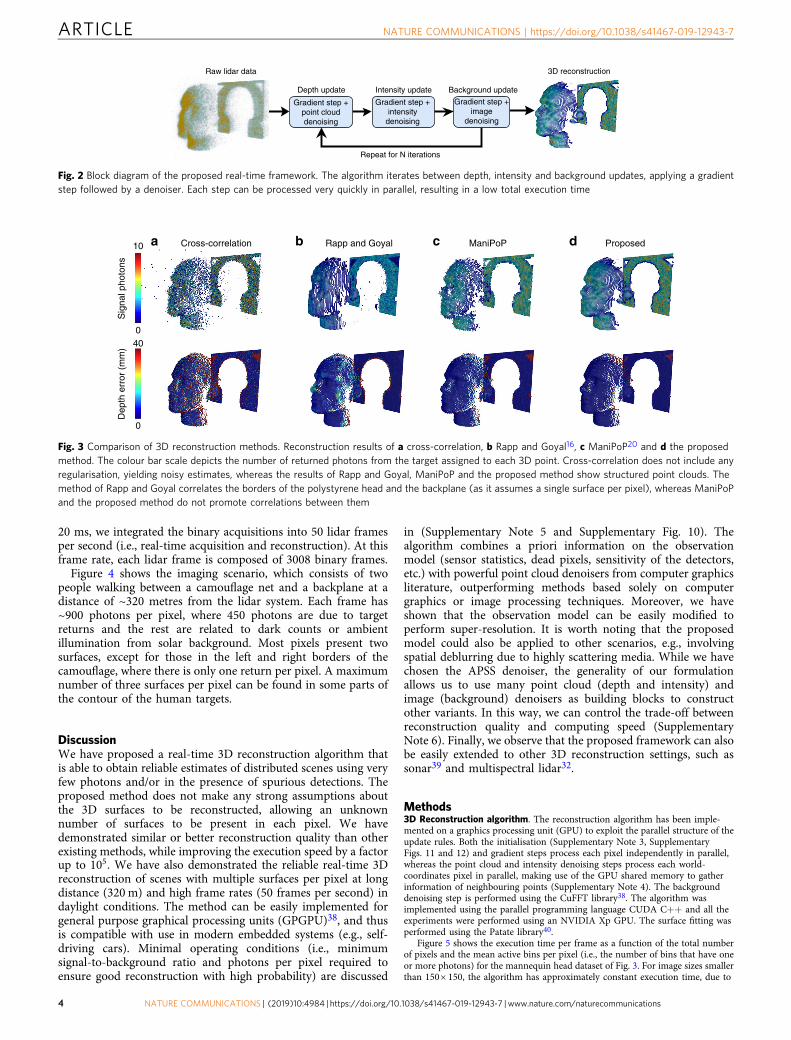
Reconstruction algorithm. The reconstruction algorithm followsthe general structure of PALM33, computing proximal gradientsteps on the blocks of variables t, r and b, as illustrated in Fig. 2.Each update first adjusts the current estimates with a gradientstep taken with respect to the log-likelihood (data-fidelity) termg t; r; bð Þ, followed by an off-the-shelf denoising step, which playsthe role of a proximal operator34. While the gradient step takesinto account the single-photon lidar observation model (i.e.,Poisson statistics, presence of dead pixels, compressive sensing,etc.), the denoising step profits from off-the-shelf point clouddenoisers. A summary of each block update is presented below,whereas an in-detail explanation of the full algorithm can befound in (Supplementary Notes 1–3).

Depth update: A gradient step is taken with respect to thedepth variables t and the point cloud Φ is denoised with thealgebraic point set surfaces (APSS) algorithm35,36 working in thereal-world coordinate system. APSS fits a smooth continuoussurface to the set of points defined by t, using spheres as localprimitives (Supplementary Fig. 1). The fitting is controlled by akernel, whose size adjusts the degree of low-pass filtering of thesurface (Supplementary Fig. 2). In contrast to conventional depthimage regularisation/denoisers, the point cloud denoiser canhandle an arbitrary number of surfaces per pixel, regardless of thepixel format of the lidar system. Moreover, all of the 3D pointsare processed in parallel, equating to very low execution times.

Intensity update: In this update, the gradient step is taken withrespect to r, followed by a denoising step using the manifoldmetrics defined by Φ in real-world coordinates. In this way, weonly consider correlations between points within the samesurface. A low-pass filter is applied using the nearest neighboursof each point (Supplementary Fig. 3), as in ISOMAP37. This stepalso processes all the points in parallel, only accounting for localcorrelations. After the denoising step, we remove the points withintensity lower than a given threshold, which is set as theminimum admissible reflectivity (normalised intensity) (Supple-mentary Fig. 4).

Background update: In a similar fashion to the intensity anddepth updates, a gradient step is taken with respect to b. Here, theproximal operator depends on the characteristics of the lidarsystem. In bistatic raster-scanning systems, the laser source andsingle-photon detectors are not co-axial and background countsare not necessarily spatially correlated. Consequently, no spatialregularisation is applied to the background. In this case, thedenoising operator reduces to the identity, i.e., no denoising. Inmonostatic raster-scanning systems and lidar arrays, the

background detections resemble a passive image. In this case,spatial regularisation is useful to improve the estimates(Supplementary Fig. 5). Thus, we replace the proximal operatorwith an off-the-shelf image denoising algorithm. Specifically, wechoose a simple denoiser based on the fast Fourier transform(FFT), which has low computational complexity.

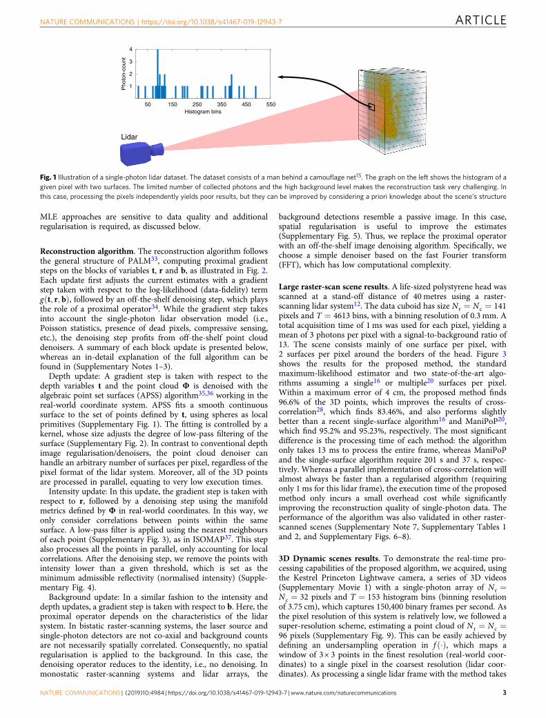
Large raster-scan scene results. A life-sized polystyrene head wasscanned at a stand-off distance of 40 metres using a raster-scanning lidar system12. The data cuboid has size Nr ¼ Nc ¼ 141pixels and T ¼ 4613 bins, with a binning resolution of 0.3 mm. Atotal acquisition time of 1 ms was used for each pixel, yielding amean of 3 photons per pixel with a signal-to-background ratio of13. The scene consists mainly of one surface per pixel, with2 surfaces per pixel around the borders of the head. Figure 3shows the results for the proposed method, the standardmaximum-likelihood estimator and two state-of-the-art algo-rithms assuming a single16 or multiple20 surfaces per pixel.Within a maximum error of 4 cm, the proposed method finds96.6% of the 3D points, which improves the results of cross-correlation28, which finds 83.46%, and also performs slightlybetter than a recent single-surface algorithm16 and ManiPoP20,which find 95.2% and 95.23%, respectively. The most significantdifference is the processing time of each method: the algorithmonly takes 13 ms to process the entire frame, whereas ManiPoPand the single-surface algorithm require 201 s and 37 s, respec-tively. Whereas a parallel implementation of cross-correlation willalmost always be faster than a regularised algorithm (requiringonly 1 ms for this lidar frame), the execution time of the proposedmethod only incurs a small overhead cost while significantlyimproving the reconstruction quality of single-photon data. Theperformance of the algorithm was also validated in other raster-scanned scenes (Supplementary Note 7, Supplementary Tables 1and 2, and Supplementary Figs. 6–8).

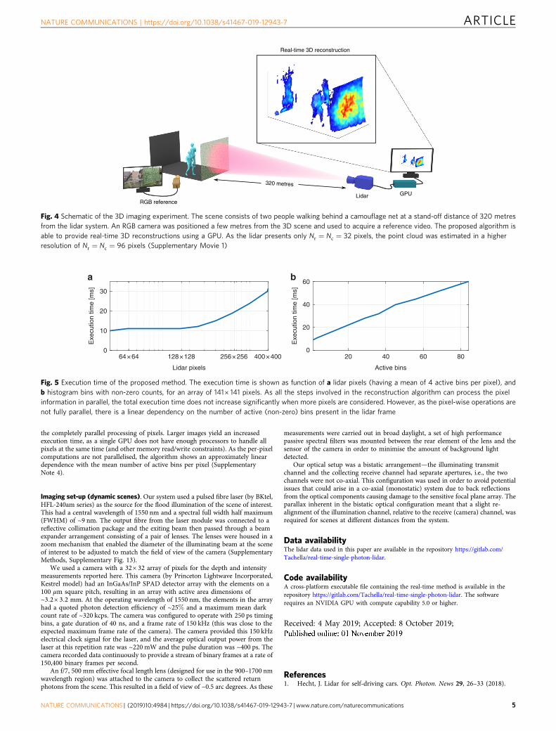
3D Dynamic scenes results. To demonstrate the real-time pro-cessing capabilities of the proposed algorithm, we acquired, usingthe Kestrel Princeton Lightwave camera, a series of 3D videos(Supplementary Movie 1) with a single-photon array of Nr ¼Nc ¼ 32 pixels and T ¼ 153 histogram bins (binning resolutionof 3.75 cm), which captures 150,400 binary frames per second. Asthe pixel resolution of this system is relatively low, we followed asuper-resolution scheme, estimating a point cloud of Nr ¼ Nc ¼96 pixels (Supplementary Fig. 9). This can be easily achieved bydefining an undersampling operation in f ð�Þ, which maps awindow of 3 ´ 3 points in the finest resolution (real-world coor-dinates) to a single pixel in the coarsest resolution (lidar coor-dinates). As processing a single lidar frame with the method takes

1

2

3

4

Pho

ton-

coun

t

50 150 250 350 450 550Histogram bins

Lidar

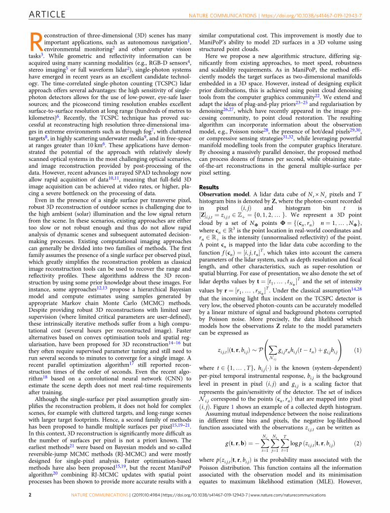
Fig. 1 Illustration of a single-photon lidar dataset. The dataset consists of a man behind a camouflage net15. The graph on the left shows the histogram of agiven pixel with two surfaces. The limited number of collected photons and the high background level makes the reconstruction task very challenging. Inthis case, processing the pixels independently yields poor results, but they can be improved by considering a priori knowledge about the scene’s structure

NATURE COMMUNICATIONS | https://doi.org/10.1038/s41467-019-12943-7 ARTICLE

NATURE COMMUNICATIONS | (2019) 10:4984 | https://doi.org/10.1038/s41467-019-12943-7 | www.nature.com/naturecommunications 3

20 ms, we integrated the binary acquisitions into 50 lidar framesper second (i.e., real-time acquisition and reconstruction). At thisframe rate, each lidar frame is composed of 3008 binary frames.

Figure 4 shows the imaging scenario, which consists of twopeople walking between a camouflage net and a backplane at adistance of ~320 metres from the lidar system. Each frame has~900 photons per pixel, where 450 photons are due to targetreturns and the rest are related to dark counts or ambientillumination from solar background. Most pixels present twosurfaces, except for those in the left and right borders of thecamouflage, where there is only one return per pixel. A maximumnumber of three surfaces per pixel can be found in some parts ofthe contour of the human targets.

DiscussionWe have proposed a real-time 3D reconstruction algorithm thatis able to obtain reliable estimates of distributed scenes using veryfew photons and/or in the presence of spurious detections. Theproposed method does not make any strong assumptions aboutthe 3D surfaces to be reconstructed, allowing an unknownnumber of surfaces to be present in each pixel. We havedemonstrated similar or better reconstruction quality than otherexisting methods, while improving the execution speed by a factorup to 105. We have also demonstrated the reliable real-time 3Dreconstruction of scenes with multiple surfaces per pixel at longdistance (320 m) and high frame rates (50 frames per second) indaylight conditions. The method can be easily implemented forgeneral purpose graphical processing units (GPGPU)38, and thusis compatible with use in modern embedded systems (e.g., self-driving cars). Minimal operating conditions (i.e., minimumsignal-to-background ratio and photons per pixel required toensure good reconstruction with high probability) are discussed

in (Supplementary Note 5 and Supplementary Fig. 10). Thealgorithm combines a priori information on the observationmodel (sensor statistics, dead pixels, sensitivity of the detectors,etc.) with powerful point cloud denoisers from computer graphicsliterature, outperforming methods based solely on computergraphics or image processing techniques. Moreover, we haveshown that the observation model can be easily modified toperform super-resolution. It is worth noting that the proposedmodel could also be applied to other scenarios, e.g., involvingspatial deblurring due to highly scattering media. While we havechosen the APSS denoiser, the generality of our formulationallows us to use many point cloud (depth and intensity) andimage (background) denoisers as building blocks to constructother variants. In this way, we can control the trade-off betweenreconstruction quality and computing speed (SupplementaryNote 6). Finally, we observe that the proposed framework can alsobe easily extended to other 3D reconstruction settings, such assonar39 and multispectral lidar32.

Methods3D Reconstruction algorithm. The reconstruction algorithm has been imple-mented on a graphics processing unit (GPU) to exploit the parallel structure of theupdate rules. Both the initialisation (Supplementary Note 3, SupplementaryFigs. 11 and 12) and gradient steps process each pixel independently in parallel,whereas the point cloud and intensity denoising steps process each world-coordinates pixel in parallel, making use of the GPU shared memory to gatherinformation of neighbouring points (Supplementary Note 4). The backgrounddenoising step is performed using the CuFFT library38. The algorithm wasimplemented using the parallel programming language CUDA C++ and all theexperiments were performed using an NVIDIA Xp GPU. The surface fitting wasperformed using the Patate library40.

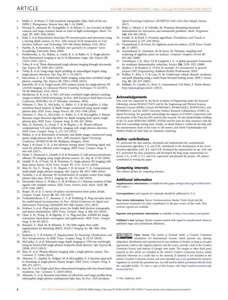
Figure 5 shows the execution time per frame as a function of the total numberof pixels and the mean active bins per pixel (i.e., the number of bins that have oneor more photons) for the mannequin head dataset of Fig. 3. For image sizes smallerthan 150 ´ 150, the algorithm has approximately constant execution time, due to

ManiPoPCross-correlation Rapp and Goyal Proposed

0

Dep

th e

rror

(m

m)

0

Sig

nal p

hoto

ns

40

10 cba d

Fig. 3 Comparison of 3D reconstruction methods. Reconstruction results of a cross-correlation, b Rapp and Goyal16, c ManiPoP20 and d the proposedmethod. The colour bar scale depicts the number of returned photons from the target assigned to each 3D point. Cross-correlation does not include anyregularisation, yielding noisy estimates, whereas the results of Rapp and Goyal, ManiPoP and the proposed method show structured point clouds. Themethod of Rapp and Goyal correlates the borders of the polystyrene head and the backplane (as it assumes a single surface per pixel), whereas ManiPoPand the proposed method do not promote correlations between them

Gradient step +point clouddenoising

Depth update

Gradient step +intensity

denoising

Intensity update Background update

Repeat for N iterations

Raw lidar data 3D reconstruction

Gradient step +image

denoising

Fig. 2 Block diagram of the proposed real-time framework. The algorithm iterates between depth, intensity and background updates, applying a gradientstep followed by a denoiser. Each step can be processed very quickly in parallel, resulting in a low total execution time

ARTICLE NATURE COMMUNICATIONS | https://doi.org/10.1038/s41467-019-12943-7

4 NATURE COMMUNICATIONS | (2019) 10:4984 | https://doi.org/10.1038/s41467-019-12943-7 | www.nature.com/naturecommunications

the completely parallel processing of pixels. Larger images yield an increasedexecution time, as a single GPU does not have enough processors to handle allpixels at the same time (and other memory read/write constraints). As the per-pixelcomputations are not parallelised, the algorithm shows an approximately lineardependence with the mean number of active bins per pixel (SupplementaryNote 4).

Imaging set-up (dynamic scenes). Our system used a pulsed fibre laser (by BKtel,HFL-240am series) as the source for the flood illumination of the scene of interest.This had a central wavelength of 1550 nm and a spectral full width half maximum(FWHM) of ~9 nm. The output fibre from the laser module was connected to areflective collimation package and the exiting beam then passed through a beamexpander arrangement consisting of a pair of lenses. The lenses were housed in azoom mechanism that enabled the diameter of the illuminating beam at the sceneof interest to be adjusted to match the field of view of the camera (SupplementaryMethods, Supplementary Fig. 13).

We used a camera with a 32 ´ 32 array of pixels for the depth and intensitymeasurements reported here. This camera (by Princeton Lightwave Incorporated,Kestrel model) had an InGaAs/InP SPAD detector array with the elements on a100 μm square pitch, resulting in an array with active area dimensions of~3:2 ´ 3:2 mm. At the operating wavelength of 1550 nm, the elements in the arrayhad a quoted photon detection efficiency of ~25% and a maximum mean darkcount rate of ~320 kcps. The camera was configured to operate with 250 ps timingbins, a gate duration of 40 ns, and a frame rate of 150 kHz (this was close to theexpected maximum frame rate of the camera). The camera provided this 150 kHzelectrical clock signal for the laser, and the average optical output power from thelaser at this repetition rate was ~220 mW and the pulse duration was ~400 ps. Thecamera recorded data continuously to provide a stream of binary frames at a rate of150,400 binary frames per second.

An f/7, 500 mm effective focal length lens (designed for use in the 900–1700 nmwavelength region) was attached to the camera to collect the scattered returnphotons from the scene. This resulted in a field of view of ~0.5 arc degrees. As these

measurements were carried out in broad daylight, a set of high performancepassive spectral filters was mounted between the rear element of the lens and thesensor of the camera in order to minimise the amount of background lightdetected.

Our optical setup was a bistatic arrangement—the illuminating transmitchannel and the collecting receive channel had separate apertures, i.e., the twochannels were not co-axial. This configuration was used in order to avoid potentialissues that could arise in a co-axial (monostatic) system due to back reflectionsfrom the optical components causing damage to the sensitive focal plane array. Theparallax inherent in the bistatic optical configuration meant that a slight re-alignment of the illumination channel, relative to the receive (camera) channel, wasrequired for scenes at different distances from the system.

Data availabilityThe lidar data used in this paper are available in the repository https://gitlab.com/Tachella/real-time-single-photon-lidar.

Code availabilityA cross-platform executable file containing the real-time method is available in therepository https://gitlab.com/Tachella/real-time-single-photon-lidar. The softwarerequires an NVIDIA GPU with compute capability 5.0 or higher.

Received: 4 May 2019; Accepted: 8 October 2019;

References1. Hecht, J. Lidar for self-driving cars. Opt. Photon. News 29, 26–33 (2018).

20 40 60 80

Active bins

0

20

40

60

Exe

cutio

n tim

e [m

s]

64×64 128×128 256×256 400×400

Lidar pixels

0

10

20

30

Exe

cutio

n tim

e [m

s]

a b

Fig. 5 Execution time of the proposed method. The execution time is shown as function of a lidar pixels (having a mean of 4 active bins per pixel), andb histogram bins with non-zero counts, for an array of 141 ´ 141 pixels. As all the steps involved in the reconstruction algorithm can process the pixelinformation in parallel, the total execution time does not increase significantly when more pixels are considered. However, as the pixel-wise operations arenot fully parallel, there is a linear dependency on the number of active (non-zero) bins present in the lidar frame

RGB referenceLidar GPU

320 metres

Real-time 3D reconstruction

Fig. 4 Schematic of the 3D imaging experiment. The scene consists of two people walking behind a camouflage net at a stand-off distance of 320 metresfrom the lidar system. An RGB camera was positioned a few metres from the 3D scene and used to acquire a reference video. The proposed algorithm isable to provide real-time 3D reconstructions using a GPU. As the lidar presents only Nr ¼ Nc ¼ 32 pixels, the point cloud was estimated in a higherresolution of Nr ¼ Nc ¼ 96 pixels (Supplementary Movie 1)

NATURE COMMUNICATIONS | https://doi.org/10.1038/s41467-019-12943-7 ARTICLE

NATURE COMMUNICATIONS | (2019) 10:4984 | https://doi.org/10.1038/s41467-019-12943-7 | www.nature.com/naturecommunications 5

2. Mallet, C. & Bretar, F. Full-waveform topographic lidar: State-of-the-art.ISPRS J. Photogramm. Remote Sens. 64, 1–16 (2009).

3. Horaud, R., Hansard, M., Evangelidis, G. & Ménier, C. An overview of depthcameras and range scanners based on time-of-flight technologies. Mach. Vis.Appl. 27, 1005–1020 (2016).

4. Izadi, S. et al. Kinectfusion: Real-time 3D reconstruction and interaction usinga moving depth camera. In Proc. 24th Annual ACM Symposium on UserInterface Software and Technology 559–568 (Santa Barbara, USA, 2011).

5. Hartley, R. & Zisserman, A. Multiple view geometry in computer vision(Cambridge University Press, 2003).

6. Pawlikowska, A. M., Halimi, A., Lamb, R. A. & Buller, G. S. Single-photonthree-dimensional imaging at up to 10 kilometers range. Opt. Express 25,11919–11931 (2017).

7. Tobin, R. et al. Three-dimensional single-photon imaging through obscurants.Opt. Express 27, 4590–4611 (2019).

8. Tobin, R. et al. Long-range depth profiling of camouflaged targets usingsingle-photon detection. Opt. Eng. 57, 1–10 (2017).

9. Maccarone, A. et al. Underwater depth imaging using time-correlated single-photon counting. Opt. Express 23, 33911–33926 (2015).

10. Entwistle, M. et al. Geiger-mode APD camera system for single-photon 3DLADAR imaging. In Advanced Photon Counting Techniques VI vol 8375,78–89 (Baltimore, USA, 2012).

11. Henderson, R. K. et al. A 192 ´ 128 time correlated single photon countingimager in 40nm CMOS technology. In Proc. 44th European Solid State CircuitsConference (ESSCIRC) 54–57 (Dresden, Germany, 2018).

12. Altmann, Y., Ren, X., McCarthy, A., Buller, G. S. & McLaughlin, S. Lidarwaveform-based analysis of depth images constructed using sparse single-photon data. IEEE Trans. Image Process. 25, 1935–1946 (2016).

13. Altmann, Y., Ren, X., McCarthy, A., Buller, G. S. & McLaughlin, S. RobustBayesian target detection algorithm for depth imaging from sparse single-photon data. IEEE Trans. Comput. Imag. 2, 456–467 (2016).

14. Shin, D., Kirmani, A., Goyal, V. K. & Shapiro, J. H. Photon-efficientcomputational 3-D and reflectivity imaging with single-photon detectors.IEEE Trans. Comput. Imag. 1, 112–125 (2015).

15. Halimi, A. et al. Restoration of intensity and depth images constructed usingsparse single-photon data. In Proc. 24th European Signal ProcessingConference (EUSIPCO) 86–90 (Budapest, Hungary, 2016).

16. Rapp, J. & Goyal, V. K. A few photons among many: Unmixing signal andnoise for photon-efficient active imaging. IEEE Trans. Comput. Imag. 3,445–459 (2017).

17. Heide, F., Diamond, S., Lindell, D. B. & Wetzstein, G. Sub-picosecond photon-efficient 3D imaging using single-photon sensors. Sci. Rep. 8, 17726 (2018).

18. Lindell, D. B., O’Toole, M. & Wetzstein, G. Single-photon 3D imaging withdeep sensor fusion. ACM Trans. Graph. 37, 113:1–113:12 (2018).

19. Shin, D., Xu, F., Wong, F. N., Shapiro, J. H. & Goyal, V. K. Computationalmulti-depth single-photon imaging. Opt. Express 24, 1873–1888 (2016).

20. Tachella, J. et al. Bayesian 3D reconstruction of complex scenes from single-photon lidar data. SIAM J. Imaging Sci. 12, 521–550 (2019).

21. Hernandez-Marin, S., Wallace, A. M. & Gibson, G. J. Bayesian analysis of lidarsignals with multiple returns. IEEE Trans. Pattern Anal. Mach. Intell. 29,2170–2180 (2007).

22. Berger, M. et al. A survey of surface reconstruction from point clouds.Comput. Graph. Forum 36, 301–329 (2017).

23. Venkatakrishnan, S. V., Bouman, C. A. & Wohlberg, B. Plug-and-play priorsfor model based reconstruction. In Proc. Global Conference on Signal andInformation Processing (GlobalSIP) 945–948 (Austin, USA, 2013).

24. Sreehari, S. et al. Plug-and-play priors for bright field electron tomographyand sparse interpolation. IEEE Trans. Comput. Imag. 2, 408–423 (2016).

25. Chan, S. H., Wang, X. & Elgendy, O. A. Plug-and-play ADMM for imagerestoration: fixed-point convergence and applications. IEEE Trans. Comput.Imag. 3, 84–98 (2017).

26. Romano, Y., Elad, M. & Milanfar, P. The little engine that could:regularization by denoising (RED). SIAM J. Imaging Sci. 10, 1804–1844(2017).

27. Reehorst, E. T. & Schniter, P. Regularization by Denoising: Clarifications andNew Interpretations. In IEEE Trans. Comput. Imag. 5, 52–67 (2019).

28. McCarthy, A. et al. Kilometer-range depth imaging at 1550 nm wavelengthusing an InGaAs/InP single-photon avalanche diode detector. Opt. Express 21,22098–22113 (2013).

29. Shin, D. et al. Photon-efficient imaging with a single-photon camera. Nat.Commun. 7, 12046 (2016).

30. Altmann, Y., Aspden, R., Padgett, M. & McLaughlin, S. A bayesian approachto denoising of single-photon binary images. IEEE Trans. Comput. Imag. 3,460–471 (2017).

31. Sun, M.-J. et al. Single-pixel three-dimensional imaging with time-based depthresolution. Nat. Commun. 7, 12010 (2016).

32. Altmann, Y. et al. Bayesian restoration of reflectivity and range profiles fromsubsampled single-photon multispectral lidar data. In Proc. 25th European

Signal Processing Conference (EUSIPCO) 1410–1414 (Kos Island, Greece,2017).

33. Bolte, J., Sabach, S. & Teboulle, M. Proximal alternating linearizedminimization for nonconvex and nonsmooth problems. Math. Programm.146, 459–494 (2014).

34. Parikh, N. & Boyd, S. Proximal algorithms. Foundations and Trends inOptimization 1, 127–239 (2014).

35. Guennebaud, G. & Gross, M. Algebraic point set surfaces. ACM Trans. Graph.26, 23 (2007).

36. Guennebaud, G., Germann, M. & Gross, M. Dynamic sampling andrendering of algebraic point set surfaces. Computer Graphics Forum 27,653–662 (2008).

37. Tenenbaum, J. B., Silva, Vd & Langford, J. C. A global geometric frameworkfor nonlinear dimensionality reduction. Science 290, 2319–2323 (2000).

38. Sanders, J. & Kandrot, E. CUDA by example: An introduction to general-purpose GPU programming (Addison-Wesley Professional, 2010).

39. Petillot, Y., Ruiz, I. T. & Lane, D. M. Underwater vehicle obstacle avoidanceand path planning using a multi-beam forward looking sonar. IEEE J. Ocean.Eng. 26, 240–251 (2001).

40. Mellado, N., Ciaudo, G., Boyé, S., Guennebaud, G.& Barla, P. Patate library.http://patate.gforge.inria.fr/ (2013).

AcknowledgementsThis work was supported by the Royal Academy of Engineering under the ResearchFellowship scheme RF201617/16/31 and by the Engineering and Physical SciencesResearch Council (EPSRC) Grants EP/N003446/1, EP/M01326X/1, EP/K015338/1, andEP/S000631/1, and the MOD University Defence Research Collaboration (UDRC) inSignal Processing. We gratefully acknowledge the support of NVIDIA Corporation withthe donation of the Titan Xp GPU used for this research. We also thank Bradley Schillingof the US Army RDECOM CERDEC NVESD and his team for their assistance with thefield trial (camouflage netting data). Finally, we thank Robert J. Collins for his help withthe measurements made of the scene at 320 metres, and David Vanderhaeghe andMathias Paulin for their help on volumetric rendering.

Author contributionsJ.T. performed the data analysis, developed and implemented the computationalreconstruction algorithm; Y.A. and N.M. contributed to the development of the recon-struction algorithm; A.M., R.T. and G.S.B. developed the experimental set-up; A.M. andR.T. performed the data acquisition and developed the long-range experimental sce-narios; Y.A., G.S.B., J.-Y.T. and S.M. supervised and planned the project. All authorscontributed to writing the paper.

Competing interestsThe authors declare no competing interests.

Additional informationSupplementary information is available for this paper at https://doi.org/10.1038/s41467-019-12943-7.

Correspondence and requests for materials should be addressed to Y.A.

Peer review information Nature Communications thanks Vivek Goyal and theanonymous reviewer(s) for their contribution to the peer review of this work. Peerreviewer reports are available.

Reprints and permission information is available at http://www.nature.com/reprints

Publisher’s note Springer Nature remains neutral with regard to jurisdictional claims inpublished maps and institutional affiliations.

Open Access This article is licensed under a Creative CommonsAttribution 4.0 International License, which permits use, sharing,

adaptation, distribution and reproduction in any medium or format, as long as you giveappropriate credit to the original author(s) and the source, provide a link to the CreativeCommons license, and indicate if changes were made. The images or other third partymaterial in this article are included in the article’s Creative Commons license, unlessindicated otherwise in a credit line to the material. If material is not included in thearticle’s Creative Commons license and your intended use is not permitted by statutoryregulation or exceeds the permitted use, you will need to obtain permission directly fromthe copyright holder. To view a copy of this license, visit http://creativecommons.org/licenses/by/4.0/.

© The Author(s) 2019

ARTICLE NATURE COMMUNICATIONS | https://doi.org/10.1038/s41467-019-12943-7

6 NATURE COMMUNICATIONS | (2019) 10:4984 | https://doi.org/10.1038/s41467-019-12943-7 | www.nature.com/naturecommunications