Real Interest Rate Is Falling Macroeconomic …myweb.liu.edu/~uroy/resume/myPDF/JEE-2015.pdfdemand curve becomes a kinked curve with a negatively sloped segment (when the ZLB is non-

Full Terms & Conditions of access and use can be found athttp://www.tandfonline.com/action/journalInformation?journalCode=vece20

Download by: [LIU Libraries], [Professor Udayan Roy] Date: 13 September 2015, At: 12:53

The Journal of Economic Education

ISSN: 0022-0485 (Print) 2152-4068 (Online) Journal homepage: http://www.tandfonline.com/loi/vece20

Macroeconomic Stabilization When the NaturalReal Interest Rate Is Falling

Sebastien Buttet & Udayan Roy

To cite this article: Sebastien Buttet & Udayan Roy (2015) Macroeconomic Stabilization Whenthe Natural Real Interest Rate Is Falling, The Journal of Economic Education, 46:4, 376-393, DOI:10.1080/00220485.2015.1071218

To link to this article: http://dx.doi.org/10.1080/00220485.2015.1071218

Accepted online: 15 Jul 2015.

Submit your article to this journal

Article views: 4

View related articles

View Crossmark data

THE JOURNAL OF ECONOMIC EDUCATION, 46(4), 376–393, 2015Copyright C© Taylor & Francis Group, LLCISSN: 0022-0485 / 2152-4068 onlineDOI: 10.1080/00220485.2015.1071218

CONTENT ARTICLE IN ECONOMICS

Macroeconomic Stabilization When the Natural RealInterest Rate Is Falling

Sebastien Buttet and Udayan Roy

The authors modify the Dynamic Aggregate Demand-Dynamic Aggregate Supply model in Mankiw’swidely used intermediate macroeconomics textbook to discuss monetary policy when the natural realinterest rate is falling over time. Their results highlight a new role for the central bank’s inflationtarget as a tool of macroeconomic stabilization. They show that even when the zero lower bound isnot binding, a prudent central bank must match every decrease in the natural real interest rate with anequal increase in the target rate of inflation in order to stabilize the risk of the economy falling into adeflationary spiral, which is an acute case of simultaneously falling output and inflation in which theeconomy’s self-correcting forces are inactive.

Keywords intermediate macroeconomics, natural interest rate, secular stagnation, zero lower bound

JEL codes E12, E52, E58

Recent discussions of secular stagnation have drawn attention to the steady decrease in thenatural real interest rate in the United States since the 1980s.1 In this article, we investigate howa nation’s central bank should respond to decreases in the natural real interest rate when thezero lower bound (ZLB) on nominal interest rates is potentially binding. In particular, if outputis at the full-employment level and inflation is at the central bank’s inflation target, should thecentral bank feel free to ignore decreases in the natural real interest rate? Our answer is no.We argue that decreases in the natural real interest rate increase an economy’s vulnerability tothe deflationary spiral, which is an acute case of simultaneously falling output and inflation inwhich the economy’s self-correcting forces become inactive. We also show that a central bankcan neutralize this danger by simply raising its inflation target.

Intermediate macroeconomics textbooks do not discuss what policymakers should do in re-sponse to changes in the natural real interest rate.2 We hope to show that a standard textbook

Sebastien Buttet (e-mail: [email protected]) is an associate professor of economics at the CityUniversity of New York, Guttman Community College. Udayan Roy (e-mail: [email protected]) is a professor ofeconomics at Long Island University. Buttet is the corresponding author.

Color versions of one or more of the figures in this article can be found online at www.tandfonline.com/vece.

Dow

nloa

ded

by [

LIU

Lib

rari

es],

[Pr

ofes

sor

Uda

yan

Roy

] at

12:

53 1

3 Se

ptem

ber

2015

TEACHING SECULAR STAGNATION 377

model and standard graphical techniques can be used to present this new aspect of macroeconomicstabilization to students. We work out the comparative static effects of a fall in the natural real in-terest rate in the Dynamic Aggregate Demand-Aggregate Supply (DAD-DAS) model of short-runmacroeconomic dynamics in Mankiw (2013, ch. 15), a widely used intermediate macroeconomicstextbook, modified, as in Buttet and Roy (2014), to formally include the ZLB on the nominalinterest rate.

In Mankiw’s DAD-DAS model, equilibrium output and inflation are determined at the intersec-tion of two curves: a negatively sloped dynamic aggregate demand curve and a positively slopeddynamic aggregate supply curve. Irrespective of the equilibrium levels of inflation and output ata given date, the economy converges over time to the model’s unique long-run equilibrium, inwhich output is at the full-employment level and inflation is at the central bank’s target rate. How-ever, when the explicit requirement that the nominal interest rate set by the central bank must benon-negative is added, Buttet and Roy (2014) show that the familiar negatively sloped aggregatedemand curve becomes a kinked curve with a negatively sloped segment (when the ZLB is non-binding) and a positively sloped segment (when the ZLB is binding).3 This leads to two (ratherthan one) long-run equilibria: (1) the stable equilibrium discussed above and (2) an unstableequilibrium at which the ZLB is binding and the slightest shock can set off a deflationary spiral.4

The equilibrium inflation rate at any given date turns out to be the crucial determinant of theeconomy’s subsequent destiny. If inflation at a given date is higher than the negative of the naturalreal interest rate, then all is well: the economy converges to the stable long-run equilibrium. If,on the other hand, inflation at a given date drops below the negative of the natural real interestrate, the economy enters a deflationary spiral. Inflation’s danger level is equal to the negative ofthe natural real interest rate; inflation must be kept above this danger level at all costs.

Consider an economy that is at the stable long-run equilibrium, with inflation equal to thecentral bank’s target inflation rate and higher than the danger level. An unfavorable demand shock(or a favorable inflation shock) could reduce inflation from the central bank’s target inflation rateto below the danger level, thereby initiating a deflationary spiral. This is why the job of the centralbank in our model is no longer restricted to the standard one of achieving full employment andlow inflation. The central bank must also do what it can to reduce the risk of a shock-induceddeflationary spiral. This is why a decrease in the natural real interest rate makes macroeconomicstabilization harder. When the natural real interest rate decreases, the negative of it increases,raising the danger level of inflation closer to the central bank’s target rate. Consequently, thepossibility that a shock would cause inflation to fall from the central bank’s target rate (in thestable equilibrium) to below the danger level becomes more likely.5

Luckily, the very nature of the danger points to a way of neutralizing it. If the risk of adeflationary spiral has increased because the danger level of inflation has increased and comescloser to the target rate, an obvious solution is to raise the target rate as well. We show that anyincrease in the economy’s vulnerability to the deflationary spiral can be neutralized by an increasein the central bank’s inflation target.6 If the natural real interest rate decreases by a certain amountand if the central bank responds by increasing the target inflation by the same amount, then thegap between the inflation target and the negative of the natural real interest rate would remainunaffected, and therefore the chance that a shock of a given size would precipitate a deflationaryspiral would stay unchanged.7

While it is fairly obvious that when the ZLB is binding, a central bank that wishes to maintainfull employment must increase its target inflation rate in lockstep with decreases in the natural

Dow

nloa

ded

by [

LIU

Lib

rari

es],

[Pr

ofes

sor

Uda

yan

Roy

] at

12:

53 1

3 Se

ptem

ber

2015

378 BUTTET AND ROY

real interest rate, the analysis outlined above shows that even when the ZLB is not binding, aprudent central bank must match every decrease in the natural real interest rate with an equalincrease in the target inflation rate in order to keep the economy’s vulnerability to the deflationaryspiral from increasing.8 Intermediate macroeconomics textbooks do not address this issue. Wehope to show that a standard textbook model and standard graphical techniques can be used topresent this new aspect of macroeconomic stabilization to students.

Note that our focus on the natural real interest rate is related to the current research anddebate on secular stagnation (e.g., Eggertsson and Mehrotra 2014). In an address to the NationalAssociation for Business Economics that is often cited in discussions of secular stagnation, LarrySummers referred to “changes in the structure of the economy that have led to a significant shift inthe natural balance between savings and investment, causing a decline in the equilibrium or normalreal rate of interest that is associated with full employment” (Summers 2014b, 69).9 However,economists do not agree on how to define secular stagnation, what causes it, or whether it existsat all (Eichengreen 2014).10 Our article shows how macroeconomic stabilization is affected bysecular stagnation as defined by Summers.

The rest of the article is organized as follows. The next section reviews historical data about realinterest rates and the output gap for the United States in the last thirty years, and proposes a simpleway to estimate the natural real interest rate for use in intermediate macroeconomics courses. Inthe following section, we present the DAD-DAS model of Mankiw (2013) modified to includethe ZLB constraint. We derive the kinked demand curve and characterize the model’s long-runequilibria and study their stability. In the subsequent two sections, we show how decreases in thenatural real interest rate increase the economy’s vulnerability to a deflationary spiral and howraising the central bank’s target inflation can insulate the economy from this danger. We concludeby discussing some issues not formally modeled in this article.

MOTIVATING EVIDENCE

A salient feature of bond markets, both in the United States and abroad, is that real interest ratesand the natural real interest rate have been in a downward trend for the past thirty years (Kingand Low 2014; Barsky, Justiniano, and Melosi 2014; Laubach and Williams 2003).11 While realinterest rates can be easily inferred from inflation and nominal yield data, the natural real interestrate is a theoretical construct that is not directly observable and must be estimated.12 Here, wepropose a model, simple enough to be included in intermediate macroeconomics courses, toestimate the natural real interest rate. We run a linear regression between real interest rates, rt ,and the output gap, �Yt

13:

rt = β0 + β1�Yt + εt (1)

where the disturbance term εt is independent and identically distributed (i.i.d.) over time. Weinterpret the estimate of the intercept β0 as an estimate of the natural real interest rate because β0

estimates the real interest rate when output gap is zero.We present estimates of β0 and β1 for each decade between 1981 and 2013 in table 1. While

our model is much simpler than Laubach and Williams (2003), we also find that the natural realinterest rate has been falling since the 1980s and has become negative after the financial crisis.14

Dow

nloa

ded

by [

LIU

Lib

rari

es],

[Pr

ofes

sor

Uda

yan

Roy

] at

12:

53 1

3 Se

ptem

ber

2015

TEACHING SECULAR STAGNATION 379

TABLE 1The Natural Real Interest Rate, 1981–2013 Quarterly Data (Std Error in Parentheses)

Decade β0 β1 R2 N

1981–1990 0.0507 −8.5510−5.36 40

(0.0041) (1.810−5)

1991–2000 0.0366 −2.1610−6.26 40

(0.0013) (5.910−6)

2001–2008 0.0184 −1.2110−5.03 32

(0.0030) (1.410−5)

2009–2013 −0.0118 −2.1110−5.16 20

(0.0104) (1.210−5)

All: 1981–2013 0.0240 −6.8810−6.06 132

(0.0021) (6.510−6)

In the next section, we present a theoretical macroeconomic model of the business cycle wherethe ZLB is potentially binding. Later, we use this model to analyze the impact of a decline in thenatural interest rate on inflation and output.

A MODEL OF MACROECONOMIC DYNAMICS

As we saw in the previous section, the natural real interest rate has been decreasing in the UnitedStates since the 1980s. We wish to show that a decrease in the natural real interest rate hasimportant implications for macroeconomic stabilization and that these implications can be easilydiscussed in undergraduate intermediate macroeconomics courses. To that end, we analyze inthe next section the comparative static effects of a decrease in the natural real interest rate usinga modified version of Mankiw’s DAD-DAS model that incorporates the ZLB on the nominalinterest rate. That modified DAD-DAS model (discussed in Buttet and Roy 2014) is summarizedin this section.

The Kinked DAD Curve

The DAD curve of the DAD-DAS model is shown in figure 1. Aggregate demand is inverselyrelated to inflation when the ZLB is nonbinding but directly related to inflation when the ZLB isbinding. To understand the kinked shape of the DAD curve, we must look at the equations thatdrive Mankiw’s DAD-DAS model. Goods market equilibrium in period t is given by

Yt = Yt − α · (rt − ρ) + εt . (2)

Here, Yt denotes the natural or long-run level of output, rt is the real interest rate, ρ is the natural orlong-run real interest rate, α is a positive parameter representing the responsiveness of aggregateexpenditure to the real interest rate, and εt represents demand shocks. Under fiscal stimulus (anincrease in government expenditure or a decrease in taxes), εt is positive; under fiscal austerity,εt is negative.15

Dow

nloa

ded

by [

LIU

Lib

rari

es],

[Pr

ofes

sor

Uda

yan

Roy

] at

12:

53 1

3 Se

ptem

ber

2015

380 BUTTET AND ROY

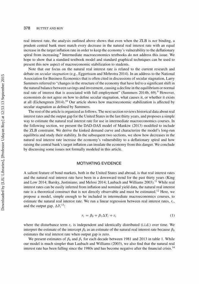
FIGURE 1 The Kinked DAD Curve. It is assumed that εt = 0 and Yt = Y for all t. The negatively sloped segment ofthe DAD curve satisfies equation (7), the positively sloped segment satisfies equation (8), and the ZLB border satisfiesequation (6)

The ex ante real interest rate in period t is determined by the Fisher equation and is equal tothe nominal interest rate it minus the inflation expected for the next period:

rt = it − Etπt+1. (3)

The expected inflation in the above equation is assumed to follow adaptive expectations:

Etπt+1 = πt . (4)

The nominal interest rate in the Fisher equation (3) is assumed to be set by the central bankaccording to its monetary policy rule. This rule is it = πt + ρ + θπ · (πt − π∗) + θY · (Yt − Yt ),where π∗ is the central bank’s inflation target, and the parameters θπ and θY are non-negative. Thenominal interest rate must obey the ZLB (i.e., it must be non-negative). Therefore, the generalizedmonetary policy rule is

it = max{0, πt + ρ + θπ · (πt − π∗) + θY · (Yt − Yt )}. (5)

Figure 1 shows the border that separates the (Yt , πt )-outcomes for which the ZLB is notbinding from the (Yt , πt )-outcomes for which the ZLB is binding. Algebraically, the monetarypolicy rule (5) implies that the ZLB border satisfies

πt + ρ + θπ · (πt − π∗) + θY · (Yt − Yt ) = 0. (6)

Above this border, the ZLB is not binding, and the nominal interest rate set by the central bankis positive (it = πt + ρ + θπ · (πt − π∗) + θY · (Yt − Yt ) > 0). On the border, the central bankchooses a zero interest rate but does so willingly, and not because it wanted a negative rate butcould not choose it. Below the border, the ZLB is binding (it = 0).

Dow

nloa

ded

by [

LIU

Lib

rari

es],

[Pr

ofes

sor

Uda

yan

Roy

] at

12:

53 1

3 Se

ptem

ber

2015

TEACHING SECULAR STAGNATION 381

Using equations (2) through (5), it is straightforward to show, following Buttet and Roy (2014),that

Yt = Yt − αθπ

1 + αθY

(πt − π∗) + 1

1 + αθY

εt (7)

when the ZLB is nonbinding and

Yt = Yt + α · (πt + ρ) + εt . (8)

when the ZLB is binding.Equation (7) is graphed in figure 1 as the negatively sloped segment of the DAD curve above

the ZLB border, which is where the ZLB is not binding. Equation (8) is graphed as the positivelysloped segment of the DAD curve below the ZLB border, which is where the ZLB is binding. Inthis way, the introduction of the ZLB on the nominal interest rate yields a kinked DAD curve.

The positively sloped segment is meant to capture the idea that falling inflation is a specialnightmare at the ZLB. As it = 0, any decline in current inflation (πt ↓) means an increase in thecurrent real interest rate (rt = it − Etπt+1 = it − πt = 0 − πt = −πt ↑). The rising real interestrate reduces aggregate demand and output (Yt ↓), as the familiar IS curve (2) dictates.16

The kinked DAD curve in figure 1 has been drawn assuming that the demand shock is absent(εt = 0). Consequently, πt = π∗ and Yt = Yt satisfy equation (7). This is point O in the figure.Similarly, it is straightforward to check that πt = −ρ and Yt = Yt satisfy equation (8). This ispoint D in the figure. Outcomes O and D will play an important role in our discussion of themodel’s equilibrium below.

The DAS Curve

Coming now to aggregate supply, inflation, πt , is determined in Mankiw’s DAD-DAS model bya conventional Phillips Curve augmented to include the role of expected inflation, Et−1πt , andan exogenous inflation shock, νt :

πt = Et−1πt + φ · (Yt − Yt ) + νt (9)

where φ is a positive parameter.When adaptive expectations (4) is substituted into the Phillips Curve (9), we get Mankiw’s

dynamic aggregate supply or DAS curve:

πt = πt−1 + φ · (Yt − Yt ) + νt . (10)

It follows that the slope of the DAS curve is dπt/dYt = φ > 0. Note also that Yt = Yt andπt = πt−1 + νt satisfy equation (10). Figure 2 shows three positively sloped DAS curves (DASO ,DASR , and DASD) for three different predetermined values of πt−1 (π∗, πR , and −ρ, respectively)and zero inflation shock (νt = 0). It follows that the heights of these three DAS curves at thefull-employment output must also be π∗, πR , and −ρ, respectively, as shown. Specifically, pointO, at which Yt = Yt and πt = π∗, must be on DASO , which is the DAS curve when πt−1 = π∗.Point D, at which Yt = Yt and πt = −ρ, must be on DASD , which is the DAS curve whenπt−1 = −ρ. In short, when there are no shocks, the height of the DAS curve at full employmentis necessarily equal to the previous period’s inflation rate.

Dow

nloa

ded

by [

LIU

Lib

rari

es],

[Pr

ofes

sor

Uda

yan

Roy

] at

12:

53 1

3 Se

ptem

ber

2015

382 BUTTET AND ROY

FIGURE 2 Points O and D are long-run equilibria, while point R is a short-run equilibrium. Both shocks are assumedzero. The DAS curves all satisfy equation (10) but for different levels of the previous period’s inflation. Note that theheight of a DAS curve at Y , the full-employment output, is equal to the previous period’s inflation rate.

Following Buttet and Roy (2014), we make the technical assumption that φ, the slope of theDAS curve, is smaller than 1/α, the slope of the positively sloped segment of the DAD curve(with ZLB binding): 1/α > φ.

Short-Run and Long-Run Equilibrium

A short-run equilibrium at any period t is graphically represented by the intersection of the DADand DAS curves for period t . Figure 2 shows three short-run equilibria (at O, R, and D) for thesame DAD curve and three different DAS curves. Let us consider these three equilibria one byone.

Unless otherwise specified, we assume that (a) there are no demand or inflation shocks(εt = νt = 0 for all t), (b) the full-employment output is constant (Yt = Y ), and (c) the parametersof the model (α, φ, ρ, θπ , θY , π∗, and Y ) are constant. We do this to focus on the dynamic forcesof change that are internal or endogenous to the economy (as opposed to change caused by shocksand parameter changes). As we saw in our subsection on the kinked DAD curve, under theseassumptions, the DAD curve does not shift over time. Therefore, let the DAD curve in figure 2be the economy’s DAD curve in all periods.

Suppose the economy is in short-run equilibrium in period t − 1 at R′′ in figure 2.17 Therefore,πt−1 = πR . Recall from our subsection on the DAS curve that under our no-shocks and constant-parameters assumptions, the height of the DAS curve at the full-employment output, Y , is equal

Dow

nloa

ded

by [

LIU

Lib

rari

es],

[Pr

ofes

sor

Uda

yan

Roy

] at

12:

53 1

3 Se

ptem

ber

2015

TEACHING SECULAR STAGNATION 383

to the predetermined rate of the previous period’s inflation. Therefore, the DAS curve in periodt must be DASR and the short-run equilibrium in period t must therefore be at R with inflationat πt = πr > πR = πt−1. This example illustrates the internal dynamics of the DAD-DAS modelwhereby change can occur (in this case, from R′′ at t − 1 to R at t) even though there are noshocks or parameter changes. (The reader can check that the short-run equilibrium at t + 1 willbe somewhere between R and O on the DAD curve and that the economy converges to O overtime.)

Next, suppose πt−1 = π∗, which is the central bank’s inflation target. Therefore, the DAScurve in period t must be DASO . Therefore, the short-run equilibrium in period t must be at O

because, as we saw in our subsections on the kinked DAD curve and the DAS curve, point O

lies on both DAD and DASO . Consequently, πt = π∗ = πt−1. In other words, O is a long-runequilibrium, which is a short-run equilibrium that repeats forever, as long as there are no shocksor parameter changes. Following Buttet and Roy (2014), we will refer to O as the orthodoxlong-run equilibrium. It can be checked that D is also a long-run equilibrium. Following Buttetand Roy (2014), we will refer to D as the deflationary long-run equilibrium.

Now that we have seen a short-run equilibrium, R, and two long-run equilibria, O and D, wecan state the stability results established by Buttet and Roy (2014). They show that if πt−1 > −ρ,then in subsequent periods inflation and output will converge to π∗ and Y , respectively. That is,if inflation in some period exceeds the negative of the natural real interest rate, there is nothing toworry about as long as there are no shocks and no parameter changes: the economy will convergeto the orthodox long-run equilibrium at O. On the other hand, if πt−1 < −ρ, then in subsequentperiods, inflation and output will decrease indefinitely, moving southwest along the DAD curveaway fron D. This is the deflationary spiral, an especially undesirable outcome.18

Having discussed the model’s equilibrium and stability properties, we next explain how afall in the natural real interest rate, which is Summers’s definition of secular stagnation, affectsinflation and output in the short and long runs.

THE EFFECTS OF A DECREASE IN THE NATURAL RATE

As the natural real interest rate ρ does not appear in equation (10), it is clear that changes in ρ

cannot shift the DAS curve. Similarly, ρ does not appear in equation (7), implying that changesin ρ cannot shift the negatively sloped segment of the DAD curve, which applies when the ZLBis not binding. We therefore have the following lemma:

Lemma 1: When the ZLB is not binding in equilibrium (short-run or long-run), a decline inthe natural real interest rate has no effect on the DAD and DAS curves. Therefore, the short-runequilibrium values of output and inflation are unaffected.

This result, when coupled with the relevant monetary policy rule it = πt + ρ + θπ · (πt −π∗) + θY · (Yt − Yt ), implies that for any decrease (respectively, increase) in the natural rate, ρ,the nominal interest rate decreases (respectively, increases) by the same percentage-point amount.Substituting adaptive expectations (4) into the Fisher equation (3) then yields the same result forthe real interest rate. In an informal sense, it is this full adjustment of the two interest rates, itand rt , to changes in ρ that makes it unnecessary for either output or inflation to adjust. There arelimits, however, to the adjustment of the nominal interest rate to a falling natural rate. Althoughρ can decrease indefinitely, the nominal interest rate cannot: it cannot fall below zero. Once ithas been driven down to zero by repeated decreases in ρ, the economy will reach the ZLB.

Dow

nloa

ded

by [

LIU

Lib

rari

es],

[Pr

ofes

sor

Uda

yan

Roy

] at

12:

53 1

3 Se

ptem

ber

2015

384 BUTTET AND ROY

FIGURE 3 The effect of a fall in the natural rate (ρ ↓) on output and inflation. It is assumed that εt = 0 and Yt = Y forall t . A falling ρ has no effect on the orthodox long-run equilibrium, O, but moves the deflationary long-run equilibriumfrom D to D′, thereby bringing the deflationary equilibrium closer to the orthodox equilibrium. The short-run equilibriummoves from Z to D′, implying decreases in both output and inflation. Had the natural real interest rate fallen even slightlybelow ρ′, a deflationary spiral would have been initiated.

For the ZLB case, note that the natural real interest rate ρ does appear in the equations for theZLB border (6) and the positively sloped segment of the DAD curve (8). It is straightforward tocheck that a decrease in ρ shifts both the ZLB border (6) and the positively sloped segment of theDAD curve upward, as shown by the dashed lines in figure 3. It is also clear from equation (8)that any decrease (respectively, increase) in ρ leads to an equal upward (respectively, downward)shift in the rising segment of the kinked DAD curve. The effects of these shifts on short-runequilibrium are shown in figure 3. The economy is initially at Z but then moves to D′. Wetherefore have the following lemma:

Lemma 2: When the ZLB on the nominal interest rate is binding in equilibrium (short-run orlong-run), a decrease in the natural real interest rate (ρ ↓) leads to decreases in both output andinflation in the short run.

To sum up, we have shown that in the short run, a fall in the natural real interest rate has noimpact on inflation and output when the ZLB is not binding, but leads to declines in inflation andoutput when the ZLB is binding.

Next, we show that a decrease in the natural real interest rate brings the (unstable) deflationarylong-run equilibrium closer to the (stable) orthodox long-run equilibrium, and thereby increasesthe likelihood that a demand and/or inflation shock might push the economy from the (stable)orthodox long-run equilibrium into a deflationary spiral.

Proposition 1: A decrease in the natural real interest rate makes an economy more vulnerableto a deflationary spiral in the sense that the minimum size, in absolute value, that a demand orinflation shock must be in order to be big enough to initiate a deflationary spiral becomes smallerwhen the natural real interest rate decreases.

Dow

nloa

ded

by [

LIU

Lib

rari

es],

[Pr

ofes

sor

Uda

yan

Roy

] at

12:

53 1

3 Se

ptem

ber

2015

TEACHING SECULAR STAGNATION 385

FIGURE 4 The natural real interest rate and the deflationary spiral-demand shock. A fall in the natural real interest ratemakes the economy more vulnerable to a deflationary spiral. It is assumed that νt = 0 and Yt = Y for all t. When thenatural real interest rate decreases, the adverse demand shock that can tip the economy into a deflationary spiral becomessmaller. When ρ = ρ1, a deflationary spiral can be initiated by the DAD curve moving to the left of DAD2. On the otherhand, when ρ = ρ2 < ρ1, the DAD curve must move only to the left of DAD3.

As in figure 1, let the DAD curve in figure 4 initially be OKD. Note that the DAD and DAScurves intersect at O, indicating that the economy is initially at the orthodox long-run equilibriumwith Yt = Y and πt = π∗. Now, consider a decrease in the natural or long-run real interest ratefrom ρ1 to ρ2 < ρ1. As in figure 3, the DAD curve shifts from OKD to OK ′D′. The deflationarylong-run equilibrium shifts from D to D′, coming closer to O, the orthodox long-run equilibrium.

From equations (7) and (8), for the negatively sloped and positively sloped segments of thekinked DAD curve, and from equation (6) for the ZLB border, it is straightforward to check thatan adverse demand shock (a decrease in εt ) shifts the kinked DAD curve to the left and leavesthe ZLB border unaffected.19 Therefore, when ρ = ρ1, if there is a big enough negative demandshock, the DAD curve could shift just to the left of DAD2 in figure 4, and thereby precipitate adeflationary spiral by reducing the inflation rate below −ρ1.20 On the other hand, when ρ = ρ2,the demand shock must only be big enough to shift the DAD curve to the left of DAD3. In otherwords, a fall in the natural real interest rate makes the economy more vulnerable to a deflationaryspiral because it reduces the size of the adverse demand shock that is just big enough to start adeflationary spiral.

We now consider the effect of an inflation shock in figure 5. Recall from the section on theDAS curve that a negative inflation shock (νt < 0) leads to a vertically downward shift of theDAS curve. When ρ = ρ1, a big enough negative (i.e., favorable) inflation shock could take theDAS curve to somewhere below DAS2, which would reduce inflation below −ρ1, and therebyinitiate a deflationary spiral. However, when ρ = ρ2 < ρ1, a smaller inflation shock would beable to initiate a deflationary spiral because the DAS curve must be pushed down only somewherebelow DAS3.

Dow

nloa

ded

by [

LIU

Lib

rari

es],

[Pr

ofes

sor

Uda

yan

Roy

] at

12:

53 1

3 Se

ptem

ber

2015

386 BUTTET AND ROY

FIGURE 5 The natural real interest rate and the deflationary spiral-inflation shock. A fall in the natural real interestrate makes the economy more vulnerable to a deflationary spiral. It is assumed that εt = 0 and Yt = Y for all t. Whenthe natural real interest rate decreases from ρ1 to ρ2, the deflationary long-run equilibrium moves from D to D′. Whenρ = ρ1, a favorable inflation shock can initiate a deflationary spiral by moving the DAS curve to below DAS2. On theother hand, when ρ = ρ2 < ρ1, the DAS curve must drop only to below DAS3.

Finally, consider an extreme scenario where the natural real interest rate decreases to suchan extent that π∗ = −ρ. Then, the two long-run equilibria collapse into the same long-runequilibrium. In figure 6, this case is represented by the DAD curve AOE2. Here, O is still thelong-run equilibrium in the sense that an economy at O remains at O in the absence of shocks,parameter changes, and policy changes. However, this long-run equilibrium is neither stable norunstable. If πt−1 > π∗ = −ρ2, then the economy will converge to O (in the absence of anyfurther shocks, parameter changes, and policy changes). However, if πt−1 < π∗ = −ρ2, then adeflationary spiral will take the economy away from O. If ρ falls further to ρ3, then −ρ3 > π∗

and the DAD curve becomes AK3E3 in figure 6. In this case, there are no long-run equilibria.For all values of πt−1, the economy will be in a deflationary spiral (in the absence of any furthershocks, parameter changes, and policy changes).

As we will show in the next section, the good news is that this extreme case can be avoidedby steadily raising the central bank’s inflation target (π∗) whenever the natural real interest ratefalls, thereby ensuring that −ρ would never catch up to π∗.

Dow

nloa

ded

by [

LIU

Lib

rari

es],

[Pr

ofes

sor

Uda

yan

Roy

] at

12:

53 1

3 Se

ptem

ber

2015

TEACHING SECULAR STAGNATION 387

FIGURE 6 If ρ falls to −π∗ or below, the economy has either one neither-stable-nor-unstable long-run equilibrium orno long-run equilibrium. It is assumed that εt = νt = 0 and Yt = Y for all t. As the natural real interest rate falls from ρ0

to ρ1 < ρ0 to ρ2 to ρ3, the DAD curve shifts from AKE to AK1E1 to AOE2 to AK3E3. For each of the first two, there aretwo long-run equilibria: O, which is stable, and the other unstable. For AOE2, O is the only long-run equilibrium, and itis neither stable nor unstable. When the DAD curve is AK3E3, there is no long-run equilibrium; the deflationary spiral isthe only possible outcome.

RAISING THE INFLATION TARGET TO NEUTRALIZE DECREASES INTHE NATURAL RATE

We have just seen in figures 4 and 5 that a decline in the natural real interest rate brings the(unstable) deflationary long-run equilibrium closer to the (stable) orthodox long-run equilibrium,thereby increasing the danger that a demand or inflation shock might push the economy fromthe orthodox long-run equilibrium into a deflationary spiral. An obvious solution is to move theorthodox long-run equilibrium in response to every move of the deflationary long-run equilibriumin such a way that a constant distance is maintained between the two.

While a decrease in ρ raises the positively sloped segment of the DAD curve (8) by the samepercentage-point amount and leaves the negatively sloped segment (7) unaffected, it can be easilychecked that an increase in π∗ raises the negatively sloped segment by the same percentage-pointamount and leaves the positively sloped segment unaffected. Therefore, as shown in figure 7, ifρ decreases by � percentage points, and simultaneously, π∗ increases by � percentage points,then the DAD curve will shift from DAD (or, OKD) to DAD2 (or, O ′K ′′D′). Therefore, while thedeflationary long-run equilibrium will move from D to D′, the orthodox long-run equilibriumwill move from O to O ′. In this way, an increase in the central bank’s inflation target insulates

Dow

nloa

ded

by [

LIU

Lib

rari

es],

[Pr

ofes

sor

Uda

yan

Roy

] at

12:

53 1

3 Se

ptem

ber

2015

388 BUTTET AND ROY

FIGURE 7 An effective way to neutralize a fall in the natural real interest rate is to raise the central bank’s inflationtarget. It is assumed that εt = νt = 0, Yt = Y for all t, and � > 0. When the natural real interest rate decreases from ρ

to ρ − �, the deflationary long-run equilibrium moves from D to D′, coming closer to the stable long-run equilibrium,O, and increasing the chance that a shock would push the economy into a deflationary spiral. However, an increase inthe central bank’s target inflation from π∗ to π∗ + � maintains the distance between the two long-run equilibria andtherefore does not allow the economy to become more vulnerable to a deflationary spiral when the natural real interestrate decreases.

the economy from the increased risk of a deflationary spiral associated with a decrease in thenatural real interest rate.

We thus have the following proposition:Proposition 2: Although a decrease in the natural real interest rate increases an economy’s

vulnerability to a deflationary spiral, the threat would be neutralized if the central bank raisesits target inflation rate by the same percentage-point amount as the decrease in the natural realinterest rate.

Dow

nloa

ded

by [

LIU

Lib

rari

es],

[Pr

ofes

sor

Uda

yan

Roy

] at

12:

53 1

3 Se

ptem

ber

2015

TEACHING SECULAR STAGNATION 389

To see the irony in this result, consider an economy that is safely ensconced at the orthodoxlong-run equilibrium with Yt = Y and πt = π∗, and then imagine steady decreases in ρ. As wesaw in lemma 1, output and inflation would be unaffected, and no danger would be apparent.Nevertheless, the probability that a sudden shock would push the economy into a deflationaryspiral would be rising all the while, in an invisible, subterranean way. Therefore, our analysissuggests that decreases in the natural real interest rate should be counteracted with matchingincreases in the central bank’s inflation target even when output is at full employment andinflation satisfies the central bank’s inflation target.

Another notable point is that a negative natural real interest rate makes it possible for aneconomy to be in a deflationary spiral even when there is no deflation! The natural real interestrate could very well drop to negative levels, as indeed our estimates in the section on motivatingevidence suggest it did in the post-2009 United States. Therefore, −ρ, the critical rate of inflationat which a deflationary spiral is triggered, could be positive. In such a situation, inflation couldbe positive and yet be low enough to trigger a deflationary spiral!

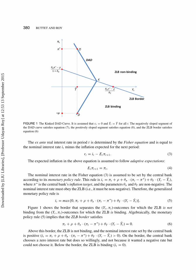
As the estimates in Laubach and Williams (2003) and our own estimates in this article suggest,the natural real interest rate has been falling in the United States since the 1980s, but nobodysaw any reason for worry at the time because output and inflation were doing fine. Our lemma1 explains why decreases in the natural real interest rate did not affect the economy back then:the ZLB on the nominal interest rate was not binding before December 2008. Our proposition 1argues that the decrease in the natural real interest rate back in the pre-December 2008 period wasmaking the economy more and more vulnerable to a deflationary spiral even though there was novisible impact on output and inflation at the time. As our proposition 2 argues, matching increasesin the Fed’s inflation target should have been implemented in the placid period before 2008.

Put another way, central banks should question the strategy of keeping inflation stable overthe long run and consider instead a strategy of keeping the nominal interest rate stable over thelong run. To see why, recall that Yt = Y and πt = π∗ in the stable orthodox long-run equilibrium.Then, from (2), the real interest rate in this equilibrium is rt = ρ, and by (5), the nominal interestrate is it = rt + πt = ρ + π∗. In line with our argument that decreases in ρ should be matchedby equal increases in π∗, it follows that ρ + π∗ should be kept constant. In other words, insteadof keeping inflation stable over the long run, central banks should consider keeping the nominalinterest rate stable over the long run.

These are new ideas in intermediate macroeconomics that follow from a standard model ina standard textbook. These ideas can be taught to intermediate macroeconomics students usingstandard graphical and algebraic techniques.

Finally, let us briefly consider how an economy that is in the orthodox long-run equilibriumwould adjust over time if and when the central bank raises its inflation target.21 Suppose at time t

the DAD curve is OKD in figure 7, the DAS is DASO , and the economy is therefore at the (stable)orthodox long-run equilibrium at O. Therefore, at t , output is Yt = Y , and inflation is πt = π∗.At time t + 1, the DAS curve would still be DASO . (Recall from our subsection on the DAScurve that the height of the DAS curve at the full-employment output is the previous period’sinflation, assuming no shocks.) However, the DAD curve at t + 1 would be DAD2, following thesimultaneous decrease in ρ by � percentage points and an equal increase in π∗. Therefore, theshort-run equilibrium at t + 1 would be at R, with Yt+1 > Y = Yt and πt+1 > π∗ = πt .

In subsequent periods, it can be shown, by following the reasoning by which we showedthe movement of the economy from R′′ to R in figure 2 in our subsection on the DAS curve,

Dow

nloa

ded

by [

LIU

Lib

rari

es],

[Pr

ofes

sor

Uda

yan

Roy

] at

12:

53 1

3 Se

ptem

ber

2015

390 BUTTET AND ROY

that the economy will over time move from R toward O ′, the new (stable) orthodox long-runequilibrium, along O ′K ′′. In short, when the central bank raises its inflation target, the economywill go immediately from O to R and then gradually from R to O ′. Output will rise above (andthen return to) the full-employment level. Inflation will rise gradually from π∗ to π∗ + �. Asfor the interest rates, it can be shown that the real interest rate will fall from rt = ρ in the initialorthodox long-run equilibrium, by more than � percentage points, to rt+1 < ρ − � and thensteadily increase to the new stable level of ρ − �. The nominal interest rate will also fall fromit = ρ + π∗ in the initial orthodox long-run equilibrium and then steadily increase to return tothe unchanged level of (ρ − �) + (π∗ + �) = ρ + π∗.

CONCLUSION

We have argued that changes in the natural real interest rate have important implications forthe conduct of macroeconomic stabilization. We have made our argument using the DAD-DASmodel in Mankiw (2013, ch. 15), modified to incorporate the ZLB on nominal interest rates. Onekey prescription for monetary policy that emerges from our analysis is that a prudent central bankshould raise its target inflation rate when the natural real interest rate decreases, irrespective ofwhether the ZLB is binding or not. A higher target inflation insulates the economy from adversedemand shocks and favorable inflation shocks that could trigger a deflationary spiral.

We end by discussing two issues that have been mentioned in recent debates but are not dis-cussed in our article. First, Summers (2013) has argued that attempts to fight negative real interestrates by raising the target inflation will lead to asset price bubbles and related financial instability.Krugman (2013) and Kocherlakota (2014) have argued that a separate set of policies (calledmacroprudential policies), aimed directly at the regulation of financial markets, are appropriateways of addressing Summers’s concerns.

Finally, both Summers (2013) and Krugman (2013) have argued in favor of prolonged fiscalstimulus as a response to secular stagnation. While aware that such fiscal stimulus would requiregovernment borrowing and increasing levels of government debt, both have argued that when realinterest rates are lower than the growth rate of real GDP, prolonged government borrowing maybe possible without any increase in the debt-to-GDP ratio, and should therefore be consideredsafe.

While we accept the importance of the issues summarized in the last two paragraphs, wewere unable to address them formally in the model that we have used in this article. Our goalthroughout has been to take a topic that is at the center of current macroeconomic debate (i.e., howto conduct monetary policy when real rates are decreasing) and show that a formal analysis of itcan be made accessible to undergraduates without requiring them to learn a whole new model.

NOTES

1. See Summers (2014a) and the collection of papers in Teulings and Baldwin (2014).2. Current editions of prominent intermediate macroeconomics textbooks (e.g., Mankiw 2013; Blanchard

and Johnson 2013; Jones 2011; and Mishkin 2011) all discuss the ZLB, and all make the pointthat expansionary fiscal policy works at the ZLB, whereas expansionary monetary policy (at leastof the conventional kind) does not. However, these textbooks do not explain the implications for

Dow

nloa

ded

by [

LIU

Lib

rari

es],

[Pr

ofes

sor

Uda

yan

Roy

] at

12:

53 1

3 Se

ptem

ber

2015

TEACHING SECULAR STAGNATION 391

macroeconomic stabilization of changes in the natural real interest rate. Carlin and Soskice (2015,Section 3.3.3) provide a detailed account of the deflationary spiral.

3. The positively sloped segment of the DAD curve captures the idea that falling inflation is a specialnightmare at the ZLB. As nominal interest rates cannot be reduced any further, any decline in inflationmeans an increase in the real interest rate, which in turn reduces aggregate demand and output.

4. Several central banks, including the Swiss National Bank, the European Central Bank, and the DanishNational Bank, have recently adopted a negative nominal interest rate policy and as a result, thezero lower bound is not a firm lower bound. Negative nominal interest rates are not an issue for ouranalysis, however, because the only assumption needed for our theoretical results to carry through isthat nominal interest rates are bounded from below. The floor value, whether positive or negative, isinconsequential. The negative nominal interest rates charged by banks reflect the cost of storage, andbecause of competitive pressure, this cost is unlikely to become much greater than 1 percent of deposit,thereby creating a floor on nominal interest rates (Cecchetti and Schoenholtz 2014).

5. In the extreme scenario where the natural real interest rate has fallen into negative territory, the economycould experience a deflationary spiral even though current inflation is positive (and presumably low).

6. Fiscal stimulus also can reverse a deflationary spiral, as shown in Buttet and Roy (2014), but taxcuts and/or increases in government purchases necessarily require increases in government borrowing,which may not always be an available option, especially in a weak economy and especially if thegovernment has already piled up so large a debt that private lenders would be leery of lending it more.Therefore, there is a need to avoid getting into a deflationary spiral in the first place, and to avoid adeflationary spiral tomorrow, it is necessary to ensure that today’s inflation stays above the negative ofthe natural real interest rate, which is the danger level.

7. Chadha and Perlman (2014), who analyzed the Gibson Paradox, note that in the presence of an uncertainnatural rate, the need to stabilize the banking sector’s reserve ratio can lead to persistent deviations ofthe market rate of interest from its natural level and consequently long-run swings in the price level.

8. Note that real interest rates have been declining in the United States since the 1980s with steadydecreases in the estimated natural real interest rate, but central banks have not raised their inflationtargets during that period. (Even the Bank of Japan’s recent move in this direction was to increase itsinflation target from 2 percent to a mere 3 percent.) This unwillingness must be reexamined in the lightof our article.

9. In his address to the National Association for Business Economics and elsewhere, Summers (2014b,67, 69) cautioned that even though the ZLB is not technically binding, low nominal and real interestrates undermine financial stability in various ways. The financial stability channel is not present in ourarticle.

10. Eichengreen (2014) emphasized four different causes of secular stagnation in his review essay: slowergrowth of technological progress (Gordon 2014); stagnant aggregate demand (Summers 2014b; Krug-man 2014); the failure of countries like the United States to invest in infrastructure, education, andtraining; and finally atrophy of skills caused by long-term unemployment and forgone on-the-job train-ing (Crafts 1989; Gordon and Krenn 2010). It would be very hard (let alone undesirable) to write anarticle which encompasses all aspects of secular stagnation, so we focus on analyzing only one aspectof secular stagnation.

11. A recent International Monetary Fund (IMF) report (IMF 2014) cited three main reasons for the declinein real rates since the mid-1980s: (a) higher saving rates in emerging market economies, (b) greaterdemand for safe assets reflecting the rapid reserve accumulation of emerging market economies as wellas increased riskiness of equity relative to bonds, and (c) a sharp and persistent decline in investmentrates in advanced economies since the global financial crisis. All three factors lead to greater savingpropensities and lower investment propensities.

12. Knut Wicksell (1898/1936, 102) offered the following definition for the natural real interest rate: “Thereis a certain rate of interest on loans which is neutral in respect to commodity prices, and tends neither toraise nor to lower them. This is necessarily the same as the rate of interest which would be determinedby supply and demand if no use were made of money and all lending were effected in the form ofreal capital goods.” More recently, Kocherlakota (2014) referred to the natural real interest rate as themandate-consistent real interest rate.

Dow

nloa

ded

by [

LIU

Lib

rari

es],

[Pr

ofes

sor

Uda

yan

Roy

] at

12:

53 1

3 Se

ptem

ber

2015

392 BUTTET AND ROY

13. Laubach and Williams (2003) used maximum likelihood to estimate changes in the natural real interestrate over time, while the equilibrium results in Barsky, Justiniano, and Melosi (2014) are derived fromsolving a dynamic utility-maximization problem. We believe that the technical and critical thinkingskills needed to fully understand these two modeling techniques are beyond the skill set that studentspossess when they take their intermediate macroeconomics courses at most colleges.

14. There are potential econometric issues with estimating changes in the natural rate using equation (1),such as co-integration of the variables, which could affect our estimates for the natural rate of interest.For the sake of space, however, and because our article proposes an innovation for intermediatemacroeconomics courses, we do not discuss econometric issues related to estimating changes inthe natural real interest rate here. Rather, we leave this discussion for an upper elective course oneconometrics or time series analysis.

15. Note that an increase in the real interest rate leads to a decrease in aggregate demand, as in the standardIS curve. For the graphical analysis in the rest of the article, we will make the simplifying assumption:γt = γ for all t.

16. The negative feedback loop between output and inflation is the mechanism that leads to a deflation-induced depression, as previously explained by Fisher (1933) and Krugman (1998). In normal times,when nominal interest rates are positive, the central bank can afford to cut interest rates followinga negative demand shock to provide short-run stimulus to the economy. When the ZLB is binding,however, cutting rates is not feasible, and real interest rates spike up as a result of lower inflation.Higher real interest rates in turn depress the economy further, which put further pressure on real rates,which depress the economy further, and so on and so forth.

17. The DAS curve through R′′ has not been drawn for simplicity.18. To see the logic behind the unstable nature of the deflationary long-run equilibrium, D, and the

deflationary spiral, see pages 46 and 47 of Buttet and Roy (2014). We saw above in figure 2 how aneconomy starting at R′′ moves to R in the next period and further towards O in subsequent periods. Itis straightforward to see the workings of the deflationary spiral by repeating that analysis, but startingat D′ instead of R′′. Buttet and Roy (2014) emphasize the need to keep inflation above −ρ, and discusshow fiscal and monetary policy can be used (a) to stop inflation from falling below −ρ and therebyprecipitating a deflationary spiral, and (b) to raise inflation above −ρ after it has already fallen belowthat level, thereby ending the deflationary spiral. They show that as the only way out of a deflationaryspiral once it has begun is fiscal stimulus. Now, fiscal stimulus usually involves a tax cut or an increasein government purchases or both, and this usually requires an increase in government borrowing. Andsuch borrowing, especially in conditions of economic weakness, may not be possible, especially for agovernment that has already borrowed a lot and is, therefore, treated warily by private lenders. That iswhy it is crucial that πt−1 < −ρ be avoided at all costs.

19. See figure 2 of Buttet and Roy (2014) for a more detailed explanation.20. Recall our discussion of the stability result in Buttet and Roy (2014): if inflation falls below the negative

of the natural real interest rate, the economy will thereafter be in a deflationary spiral (if there are nofurther shocks or parameter changes), with output and inflation falling repeatedly.

21. A detailed discussion of this dynamic adjustment is provided in Mankiw (2013, 449–53).

REFERENCES

Barsky, R., A. Justiniano, and L. Melosi. 2014. The natural rate of interest and its usefulness for monetary policy.American Economic Review: Papers and Proceedings 104 (5): 37–43.

Blanchard, O., and D. R. Johnson. 2013. Macroeconomics. 6th ed. Upper Saddle River, NJ: Prentice Hall.Buttet, S., and U. Roy. 2014. A simple treatment of the liquidity trap for intermediate macroeconomics courses. Journal

of Economic Education 45 (1): 36–55.Carlin, W., and D. Soskice. 2015. Macroeconomics: Institutions, instability, and the financial system. Oxford, UK: Oxford

University Press.Cecchetti, S., and K. L. Schoenholtz. 2014. Money, banking, and financial markets. 4th ed. New York: McGraw-Hill.

Dow

nloa

ded

by [

LIU

Lib

rari

es],

[Pr

ofes

sor

Uda

yan

Roy

] at

12:

53 1

3 Se

ptem

ber

2015

TEACHING SECULAR STAGNATION 393

Chadha, J. S., and M. Perlman. 2014. Was the Gibson paradox for real? A Wicksellian study of the relationship betweeninterest rates and prices. Financial History Review 21 (2): 139–63.

Crafts, N. 1989. Long term unemployment and the wage equation in Britain, 1925–1939. Economica 56: 247–54.Eggertsson, G. B., and N. R. Mehrotra. 2014. A model of secular stagnation. NBER Working Paper No. 20574. Cambridge,

MA: National Bureau of Economic Research.Eichengreen, B. 2014. Secular stagnation: A review of the issues. In Secular stagnation: Facts, causes, and cures, ed. C.

Teulings and R. Baldwin, 41–46. London, UK: Centre for Economic Policy Research, VoxEU.org.Fisher, I. 1933. The debt-deflation theory of great depressions. Econometrica 1 (4): 337–57.Gordon, R. J. 2014. The demise of U.S. economic growth: Restatement, rebuttal, and reflections. NBER Working Paper

No. 19895. Cambridge, MA: National Bureau of Economic Research.Gordon, R. J., and R. Krenn. 2010. The end of the Great Depression 1939–41: Policy contributions and fiscal multipliers.

NBER Working Paper No. 16380. Cambridge, MA: National Bureau of Economic Research. http://www.nber.org/papers/w16380.

International Monetary Fund (IMF). 2014. Perspectives on global real interest rates. World economic outlook: Recoverystrengthens, remains uneven, chapter 3. Washington, DC: IMF. http://www.imf.org/external/pubs/ft/weo/2014/01/pdf/c3.pdf.

Jones, C. I. 2011. Macroeconomics. 2nd ed. New York: W. W. Norton.King, M., and D. Low. 2014. Measuring the world real interest rate. NBER Working Paper No. 19887. Cambridge, MA:

National Bureau of Economic Research.Kocherlakota, N. 2014. Low real interest rates. Speech at the Ninth Annual Finance Conference, Carroll School of

Management, Boston College, Boston, Massachusetts, June 5. http://www.bis.org/review/r140606c.htm.Krugman, P. 1998. It’s baack! Japan’s slump and the return of the liquidity trap. Brookings Papers on Economic Activity

1998 (2): 137–87. Washington, DC: The Brookings Institution.———. 2013. Bubbles, regulation, and secular stagnation. The New York Times, November 16. http://krugman.blogs.

nytimes.com/2013/11/16/secular-stagnation-coalmines-bubbles-and-larry-summers/.———. 2014. Four observations on secular stagnation. In Secular stagnation: Facts, causes, and cures, ed. C. Teulings

and R. Baldwin, 61–68. London, UK: Centre for Economic Policy Research, VoxEU.org.Laubach, T., and J. C. Williams. 2003. Measuring the natural rate of interest. Review of Economics and Statistics 85 (4):

1063–70.Mankiw, G. N. 2013. Macroeconomics. 8th ed. Duffield, UK: Worth Publishers.Mishkin, F.S. 2011. Macroeconomics: Policy and practice. 1st ed. Upper Saddle River, NJ: Prentice Hall.Summers, L. H. 2013. Untitled speech. IMF Fourteenth Annual Research Conference in Honor of Stanley

Fischer, Washington, DC, November 8. http://larrysummers.com/imf-fourteenth-annual-research-conference-in-honor-of-stanley-fischer.

———. 2014a. Reflections on the new secular stagnation hypothesis. In Secular stagnation: Facts, causes, and cures,ed. C. Teulings and R. Baldwin, 27–38. London, UK: Centre for Economic Policy Research, VoxEU.org.

———. 2014b. U.S. economic prospects: Secular stagnation, hysteresis, and the zero lower bound. Business Economics49: 65–73.

Teulings, C., and R. Baldwin. 2014. Introduction. In Secular stagnation: Facts, causes, and cures, ed. C. Teulings and R.Baldwin, 1–23. London, UK: Centre for Economic Policy Research, VoxEU.org.

Wicksell, K. 1898/1936. Interest and prices. Trans. R. F. Kahn. London: Macmillan.

Dow

nloa

ded

by [

LIU

Lib

rari

es],

[Pr

ofes

sor

Uda

yan

Roy

] at

12:

53 1

3 Se

ptem

ber

2015