Real Exchange Rate, Exports, and Imports Movements: A Trivariate Analysis

The Pakistan Development Review 44 : 2 (Summer 2005) pp. 177–195

Real Exchange Rate, Exports, and Imports Movements: A Trivariate Analysis

M. ALI KEMAL and USMAN QADIR*

The exchange rate exerts a strong influence on a country’s trade. It is depicted

from the high correlation between the real exchange rate and exports (0.90) and that between the real exchange rate and imports (0.88). In the present-day scenario of falling levels of tariff and a reduced number of non-tariff barriers, the exchange rate has assumed a crucial role in influencing the trade deficit. Imports have a very significant association with exports as shown by the correlation between exports and imports (0.97). The increase in exports in the absence of surplus stocks requires an increase in production, which in turn requires capital and raw material. We analysed the long-run relationship and the short-run dynamics among the three variables. It is concluded that there exists a long-run relationship between real exchange rate, exports, and imports; and real exchange rate is negatively associated with the exports and positively associated with the imports. In the short-run, imports and exports adjust towards their equilibrium when there is disequilibrium. But the adjustment in the imports is greater than the adjustment in the exports. Moreover, exports do not respond to the shock caused by the real exchange rate, but imports respond to the sudden shock in the real exchange rate. The study ends up with the note that the sudden movements in the real exchange rate do not affect exports. Therefore, Pakistan should not worry about exchange rate shocks.

I. INTRODUCTION

There has been an increasing role of macroeconomic policies, especially the exchange rate policy, to enhance the exports and provide neutral incentives to import-competing and export-oriented industries. However, these policies have undergone significant changes over time. Countries across the globe, regardless of their level of development, are now pursuing policies that will allow them to enter the new era of globalisation and reap the benefits from such an unprecedented development in the international economic order, and Pakistan is no exception. Trade

M. Ali Kemal is Research Economist, Pakistan Institute of Development Economics, Islamabad. Usman Qadir is Staff Economist, Pakistan Institute of Development Economics, Islamabad.

Kemal and Qadir 178

is being promoted as a necessary catalyst for fostering economic growth in developing countries,1 and over the past several decades policy-makers have used the foreign trade policy and the exchange rate to influence trade flows and hence the level of economic development.

The exchange rate exerts a strong influence on a country’s trade as shown by very high correlation between the real exchange rate and exports (0.90) and that between the real exchange rate and imports (0.88). It is a major factor in determining the international competitiveness of a country. An overvaluation of the exchange rate leads to a rising trade deficit and falling reserves, which often prompt the increased use of exchange control and trade barriers, and vice versa. In the present day scenario of falling levels of tariff and a reduced number of non-tariff barriers, the exchange rate has assumed a crucial role in influencing the trade deficit.

Imports have a very significant association with exports as shown by the correlation between exports and imports (0.97). The increase in exports in the absence of surplus stocks requires an increase in production, which in turn requires capital and raw material. Less developed or developing countries are generally agro-based, labour-abundant economies with in adequate capital. Therefore, capital can only be imported from other countries to boost production.

Trade policy plays a vital role in determining the trade of a country. If we have import substitution policies, then there could be a decline in the level of imports. Conversely, if the trade is open, it could hinder the exports in short run but exports might increase in the long run. Low level of imports may cause a decline in exports due to a decline in production, and similarly a low level of exports may cause a decline in imports due to lack of foreign exchange. Therefore, developing countries would be well advised to gain a better understanding of the link between real exchange rate, exports, and imports. Our primary objective is to investigate the long-run behaviour of real exchange rate, exports, and imports of Pakistan. We shall also explore that in the short run, whether there is an adjustment towards the equilibrium path in response to a sudden shock.

The organisation of the paper is as follows. Section II discusses the theoretical underpinnings of our hypothesis and presents a review of past studies undertaken on this subject. Section III presents the data sources, methodology, and the empirical model we have used to verify our hypothesis. The evolution of the exchange rate regime and the trend of trade flows in Pakistan, descriptive analysis, and the structure of exports and imports are spelled out in Section IV. Empirical results are given in Section V, while Section VI sums up the discussion and presents the policy implications.

1The share of trade in GDP in South Asian countries has increased from 34.93 percent in the 1980s to 42.60 percent in the 1990s.

Real Exchange Rate, Exports, and Imports Movements 179

II. REVIEW OF LITERATURE

The four theoretical approaches to the analysis of the impact of devaluation on the external sector of the economy have their own arguments. Proponents of the trade/elasticities approach [Robinson (1947) and Metzler (1948)] describe the necessary and sufficient conditions for an improvement in the trade balance in terms of elasticities of demand and supply. It is argued that if the demand elasticities are sufficiently large enough and the supply elasticities sufficiently small enough, devaluation should improve the trade balance. Advocates of the absorption approach [Alexander (1952) and Johnson (1967)] describe how devaluation may change the terms of trade, increase production, switch expenditure from foreign to domestic goods, or have some other effect in reducing domestic absorption relative to production and thus improving the trade balance. International monetarists [Mundell (1971); Dornbusch (1973); Frenkel and Rodriguez (1975)] argue that devaluation reduces the real value of cash balances and/or changes the relative price of traded and non-traded goods, thus improving both the trade balance and the balance of payments, this is known as balance of payments approach. Exchange rate is also determined by the change in monetary policy [Khan (1999)], known as monetary approach. This approach postulates that the exchange rate is determined by the process of equilibrating the demand and supply of currency stocks.

Given the fact that it is not at all certain whether devaluation actually helps in improving the trade balance, a number of studies have analysed the empirical evidence on the effect of devaluations on the trade balance of a wide variety of countries. These studies initially used import and export demand elasticities to infer the response of trade flows to a price or exchange rate change, while more recent studies, constructed reduced form models that include components of all three approaches (exchange rate, income and money supply). Cooper (1971, 1971a), Connolly and Taylor (1972), Salant (1976), Himarios (1989), to name a few, found evidence to support their contention that devaluations do in general lead to an improvement in the trade balance and can thus be considered to be beneficial for the economy. However, studies by Magee (1973), Junz and Rhomberg (1973), Laffer (1976), Williamson (1983), and Bahmani-Oskooee (1985) show that in general, devaluation has an undesirable impact on the trade balance of countries.

Cointegration techniques are used alternatively to establish the long-run relationship between macroeconomic variables. Bahmani-Oskooee (1994) examines the case of Australian exports and imports, concluding that “Australia’s macroeconomic policies have indeed been effective in making exports and imports converge toward equilibrium in the long run”. Paleologos and Georgantelis (1997) use Johansen cointegration analysis to show that there is a long run relationship between the Greek trade balance and real effective exchange rate of the Greek currency. In contrast with these studies that highlight the beneficial impact of

Kemal and Qadir 180

devaluations on trade balance, there are a number of studies which show that devaluations may not have been so advantageous.

Husted (1992) uses the Engle and Granger (1987) methodology to study the long run relation between US exports and imports and found indications that the US was in violation of its inter-temporal budget constraint. In a more recent study, for a sample of four South Asian countries, Upadhayaya, et al. (1998) found that devaluation has a positive and significant effect on the trade balance in India and Nepal.

It is quite apparent that the long- and short-run relationships between exports, imports, and exchange rate do exist but the exact nature of the relationships is still not clear. The literature on the subject suggests that the trade balance improves with devaluation in some cases, while quite the opposite holds true in other cases. It is expected that the current study will make a substantial contribution to the debate on this important issue by shedding some light on the phenomenon in Pakistan for the last 22 years.

III. DATA AND METHODOLOGY Data

Monthly data is taken from December 1981 to January 2003 on exchange rate, exports, imports, domestic prices and US prices from various issues of the monthly International Financial Statistics (IFS). The cointegration test is applied on log of real exchange rate, log of imports and log of exports. Data on imports and exports are available in rupees and it is converted into dollars by dividing it by the same period’s exchange rate. Price-weighted real exchange rate is used in the analysis and is calculated by the following formula,

d

f

PPERRER *

=

where, RER denotes real exchange rate, ER denotes nominal exchange rate measured in rupee per dollar, Pf denotes foreign prices and Pd denotes domestic prices. Methodology

Our primary objective is to check the long-run and short-run relationship between the real exchange rates exports and imports. For this we used cointegration technique, which states that variables, x, y and z are said to be cointegrated if they are non-stationary but integrated of the same order and their linear combination is integrated of the order less than the order of the integration of these variables.

Engle-Granger approach and the Johansen cointegration technique are the two most popular approaches used for this analysis. However, due to some shortcomings

Real Exchange Rate, Exports, and Imports Movements 181

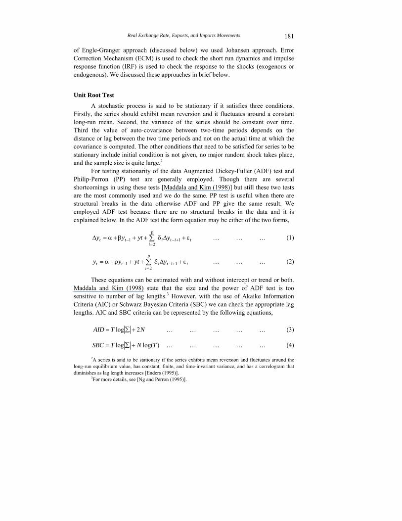
of Engle-Granger approach (discussed below) we used Johansen approach. Error Correction Mechanism (ECM) is used to check the short run dynamics and impulse response function (IRF) is used to check the response to the shocks (exogenous or endogenous). We discussed these approaches in brief below.

Unit Root Test

A stochastic process is said to be stationary if it satisfies three conditions. Firstly, the series should exhibit mean reversion and it fluctuates around a constant long-run mean. Second, the variance of the series should be constant over time. Third the value of auto-covariance between two-time periods depends on the distance or lag between the two time periods and not on the actual time at which the covariance is computed. The other conditions that need to be satisfied for series to be stationary include initial condition is not given, no major random shock takes place, and the sample size is quite large.2

For testing stationarity of the data Augmented Dickey-Fuller (ADF) test and Philip-Perron (PP) test are generally employed. Though there are several shortcomings in using these tests [Maddala and Kim (1998)] but still these two tests are the most commonly used and we do the same. PP test is useful when there are structural breaks in the data otherwise ADF and PP give the same result. We employed ADF test because there are no structural breaks in the data and it is explained below. In the ADF test the form equation may be either of the two forms,

titi

p

itt yytyy ε+∆δ++β+α=∆ +−

=− ∑ 1

21 … … … (1)

titi

p

itt yytyy ε+∆δ++ρ+α= +−

=− ∑ 1

21 … … … (2)

These equations can be estimated with and without intercept or trend or both. Maddala and Kim (1998) state that the size and the power of ADF test is too sensitive to number of lag lengths.3 However, with the use of Akaike Information Criteria (AIC) or Schwarz Bayesian Criteria (SBC) we can check the appropriate lag lengths. AIC and SBC criteria can be represented by the following equations,

NTAID 2log +∑= … … … … … (3)

)log(log TNTSBC +∑= … … … … … (4)

2A series is said to be stationary if the series exhibits mean reversion and fluctuates around the long-run equilibrium value, has constant, finite, and time-invariant variance, and has a correlogram that diminishes as lag length increases [Enders (1995)].

3For more details, see [Ng and Perron (1995)].

Kemal and Qadir 182

where Σ represents the determinant of the variance/covariance matrix of the residuals, N represents the total number of parameters estimated in all equations, and T represents the number of used observations in the regression. Minimum value of criterion is the indication that the model is better/best. Therefore there is a chance that ADF equation might not have any lagged difference variables. In ADF test, our one-tailed null and alternative hypotheses are,

HO: β = 0 or ρ = 1 (where β = ρ –1) HA: β ≠ 0 or ρ ≠ 1

Series is said to be a stationary if null hypothesis is rejected. However, if the series is not stationary at level we can check by taking the first difference of it. If the first difference is not stationary then we can take the second difference and apply the ADF test and so on. The test statistic used for the significance of coefficient is McKinnon τ-values.4

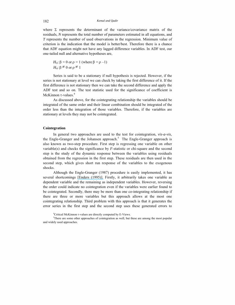
As discussed above, for the cointegrating relationship the variables should be integrated of the same order and their linear combination should be integrated of the order less than the integration of those variables. Therefore, if the variables are stationary at levels they may not be cointegrated.

Cointegration

In general two approaches are used to the test for cointegration, vis-a-vis, the Engle-Granger and the Johansen approach.5 The Engle-Granger approach is also known as two-step procedure. First step is regressing one variable on other variable(s) and checks the significance by F-statistic or chi-square and the second step is the study of the dynamic response between the variables using residuals obtained from the regression in the first step. These residuals are then used in the second step, which gives short run response of the variables to the exogenous shocks.

Although the Engle-Granger (1987) procedure is easily implemented, it has several shortcomings [Enders (1995)]. Firstly, it arbitrarily takes one variable as dependent variable and the remaining as independent variables. However, reversing the order could indicate no cointegration even if the variables were earlier found to be cointegrated. Secondly, there may be more than one co-integrating relationship if there are three or more variables but this approach allows at the most one cointegrating relationship. Third problem with this approach is that it generates the error series in the first step and the second step uses these generated errors to

4Critical McKinnon τ-values are directly computed by E-Views. 5There are some other approaches of cointegration as well, but these are among the most popular

and widely used approaches.

Real Exchange Rate, Exports, and Imports Movements 183

estimate a regression equation of error correction model. Thus the errors committed at the first step carry over to the second step.

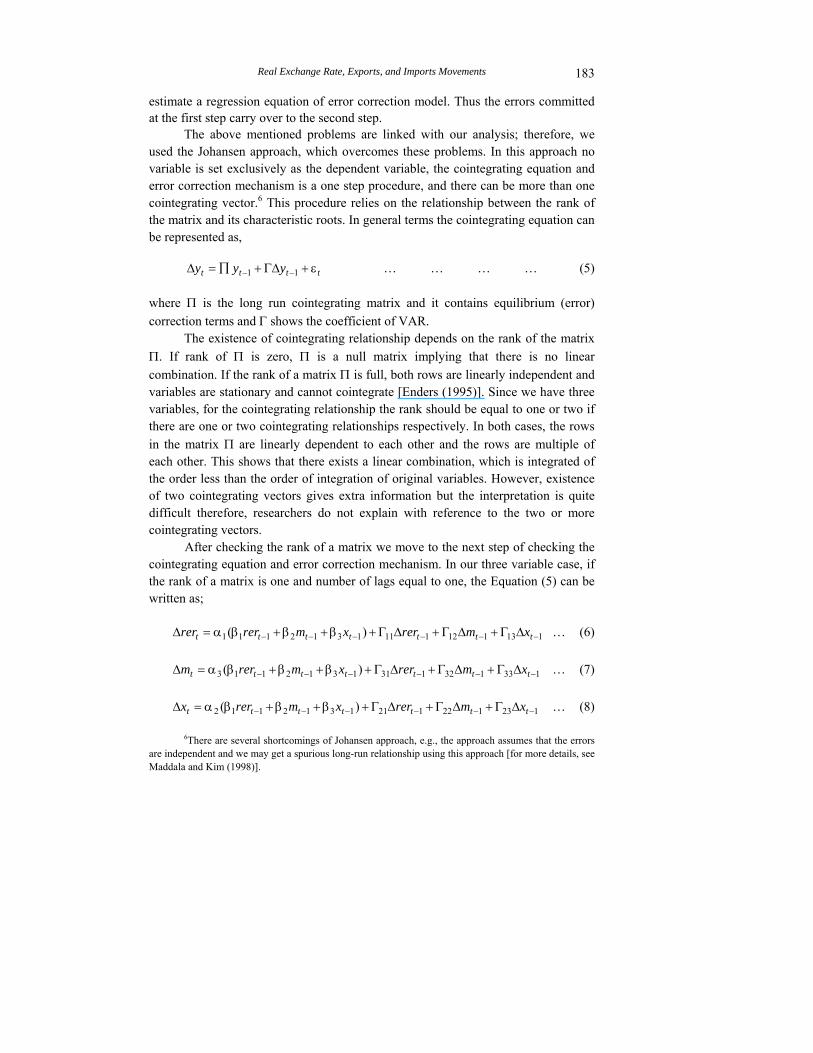
The above mentioned problems are linked with our analysis; therefore, we used the Johansen approach, which overcomes these problems. In this approach no variable is set exclusively as the dependent variable, the cointegrating equation and error correction mechanism is a one step procedure, and there can be more than one cointegrating vector.6 This procedure relies on the relationship between the rank of the matrix and its characteristic roots. In general terms the cointegrating equation can be represented as,

tttt yyy ε+Γ∆+∏=∆ −− 11 … … … … (5)

where Π is the long run cointegrating matrix and it contains equilibrium (error) correction terms and Γ shows the coefficient of VAR.

The existence of cointegrating relationship depends on the rank of the matrix Π. If rank of Π is zero, Π is a null matrix implying that there is no linear combination. If the rank of a matrix Π is full, both rows are linearly independent and variables are stationary and cannot cointegrate [Enders (1995)]. Since we have three variables, for the cointegrating relationship the rank should be equal to one or two if there are one or two cointegrating relationships respectively. In both cases, the rows in the matrix Π are linearly dependent to each other and the rows are multiple of each other. This shows that there exists a linear combination, which is integrated of the order less than the order of integration of original variables. However, existence of two cointegrating vectors gives extra information but the interpretation is quite difficult therefore, researchers do not explain with reference to the two or more cointegrating vectors.

After checking the rank of a matrix we move to the next step of checking the cointegrating equation and error correction mechanism. In our three variable case, if the rank of a matrix is one and number of lags equal to one, the Equation (5) can be written as;

1131121111312111 )( −−−−−− ∆Γ+∆Γ+∆Γ+β+β+βα=∆ ttttttt xmrerxmrerrer … (6)

1331321311312113 )( −−−−−− ∆Γ+∆Γ+∆Γ+β+β+βα=∆ ttttttt xmrerxmrerm … (7)

1231221211312112 )( −−−−−− ∆Γ+∆Γ+∆Γ+β+β+βα=∆ ttttttt xmrerxmrerx … (8)

6There are several shortcomings of Johansen approach, e.g., the approach assumes that the errors

are independent and we may get a spurious long-run relationship using this approach [for more details, see Maddala and Kim (1998)].

Kemal and Qadir 184

where rer represents log of real exchange rate, x represents log of exports and m represents log of imports. Subscript t represents the current period and ∆ represents the first difference. β1, β2, and β3 are the cointegrating vectors and α1, α2, and α3 are the coefficients of the cointegrating combination or the error correction term in the equations. However, there is a possibility that some of these terms are equal to zero. Γs are the VAR coefficients attached with each variable.

Error Correction Mechanism

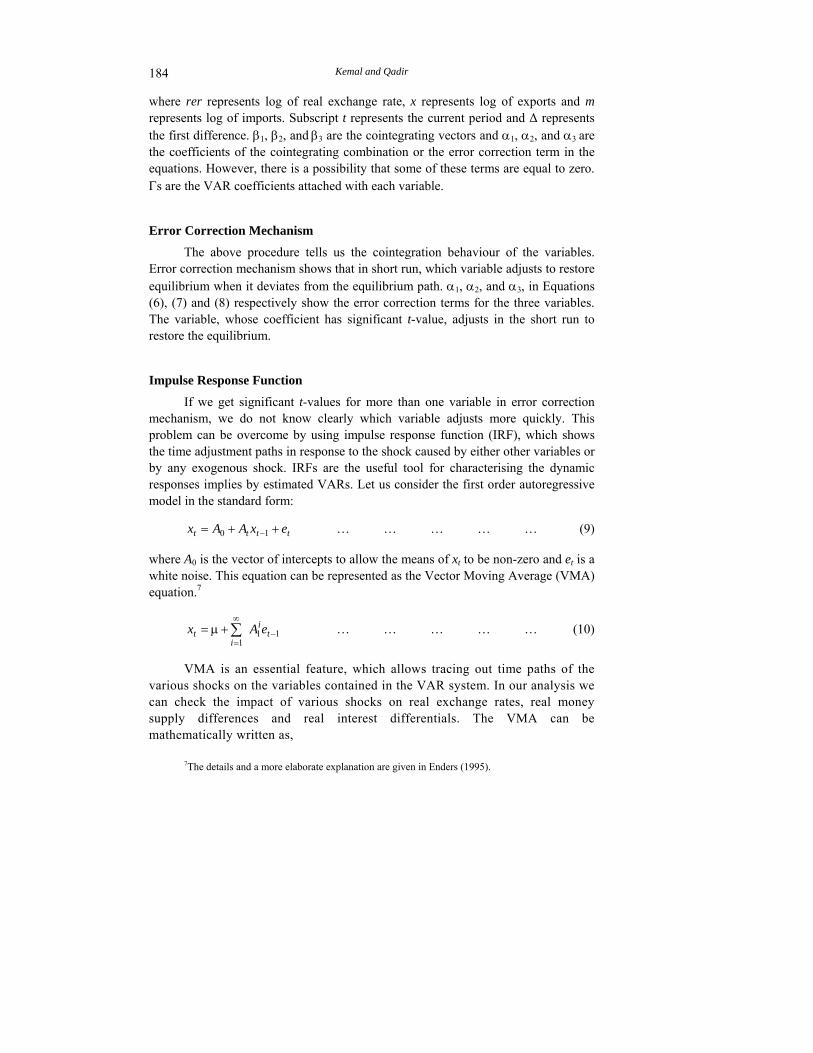
The above procedure tells us the cointegration behaviour of the variables. Error correction mechanism shows that in short run, which variable adjusts to restore equilibrium when it deviates from the equilibrium path. α1, α2, and α3, in Equations (6), (7) and (8) respectively show the error correction terms for the three variables. The variable, whose coefficient has significant t-value, adjusts in the short run to restore the equilibrium.

Impulse Response Function

If we get significant t-values for more than one variable in error correction mechanism, we do not know clearly which variable adjusts more quickly. This problem can be overcome by using impulse response function (IRF), which shows the time adjustment paths in response to the shock caused by either other variables or by any exogenous shock. IRFs are the useful tool for characterising the dynamic responses implies by estimated VARs. Let us consider the first order autoregressive model in the standard form:

tttt exAAx ++= −10 … … … … … (9)

where A0 is the vector of intercepts to allow the means of xt to be non-zero and et is a white noise. This equation can be represented as the Vector Moving Average (VMA) equation.7

111

−

∞

=∑+µ= t

i

it eAx … … … … … (10)

VMA is an essential feature, which allows tracing out time paths of the various shocks on the variables contained in the VAR system. In our analysis we can check the impact of various shocks on real exchange rates, real money supply differences and real interest differentials. The VMA can be mathematically written as,

7The details and a more elaborate explanation are given in Enders (1995).

Real Exchange Rate, Exports, and Imports Movements 185

⎥⎥⎥

⎦

⎤

⎢⎢⎢

⎣

⎡

εεε

⎥⎥⎥

⎦

⎤

⎢⎢⎢

⎣

⎡

φφφφφφφφφ

+⎥⎥⎥

⎦

⎤

⎢⎢⎢

⎣

⎡

=⎥⎥⎥

⎦

⎤

⎢⎢⎢

⎣

⎡

∑∞

=t

t

t

it

t

t

t

t

t

xmrer

iiiiiiiii

xmrer

xmrer

)()()()()()()()()(

333231

232221

131211

0

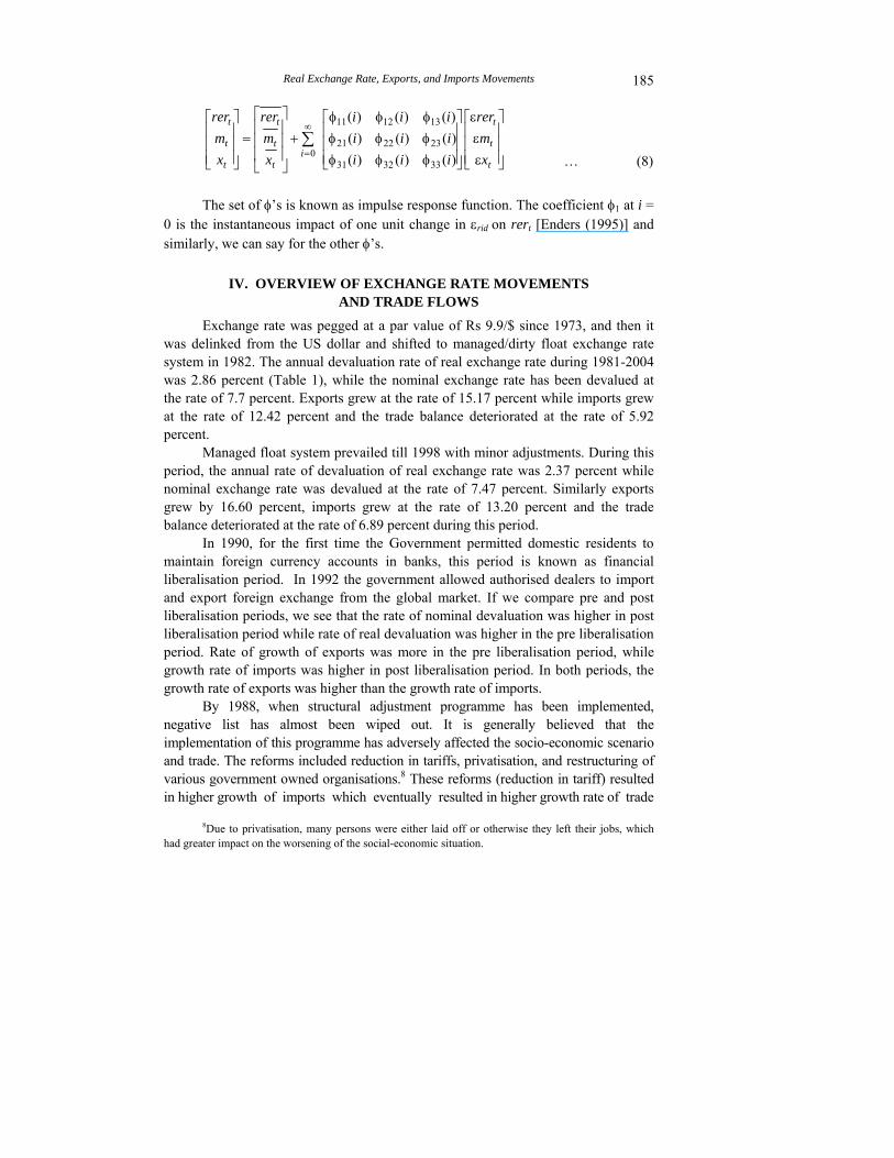
The set of φ’s is known as impulse response function. The coefficient φ1 at i = 0 is the instantaneous impact of one unit change in εrid on rert [Enders (1995)] and similarly, we can say for the other φ’s.

IV. OVERVIEW OF EXCHANGE RATE MOVEMENTS AND TRADE FLOWS

Exchange rate was pegged at a par value of Rs 9.9/$ since 1973, and then it was delinked from the US dollar and shifted to managed/dirty float exchange rate system in 1982. The annual devaluation rate of real exchange rate during 1981-2004 was 2.86 percent (Table 1), while the nominal exchange rate has been devalued at the rate of 7.7 percent. Exports grew at the rate of 15.17 percent while imports grew at the rate of 12.42 percent and the trade balance deteriorated at the rate of 5.92 percent.

Managed float system prevailed till 1998 with minor adjustments. During this period, the annual rate of devaluation of real exchange rate was 2.37 percent while nominal exchange rate was devalued at the rate of 7.47 percent. Similarly exports grew by 16.60 percent, imports grew at the rate of 13.20 percent and the trade balance deteriorated at the rate of 6.89 percent during this period.

In 1990, for the first time the Government permitted domestic residents to maintain foreign currency accounts in banks, this period is known as financial liberalisation period. In 1992 the government allowed authorised dealers to import and export foreign exchange from the global market. If we compare pre and post liberalisation periods, we see that the rate of nominal devaluation was higher in post liberalisation period while rate of real devaluation was higher in the pre liberalisation period. Rate of growth of exports was more in the pre liberalisation period, while growth rate of imports was higher in post liberalisation period. In both periods, the growth rate of exports was higher than the growth rate of imports.

By 1988, when structural adjustment programme has been implemented, negative list has almost been wiped out. It is generally believed that the implementation of this programme has adversely affected the socio-economic scenario and trade. The reforms included reduction in tariffs, privatisation, and restructuring of various government owned organisations.8 These reforms (reduction in tariff) resulted in higher growth of imports which eventually resulted in higher growth rate of trade

8Due to privatisation, many persons were either laid off or otherwise they left their jobs, which had greater impact on the worsening of the social-economic situation.

… (8)

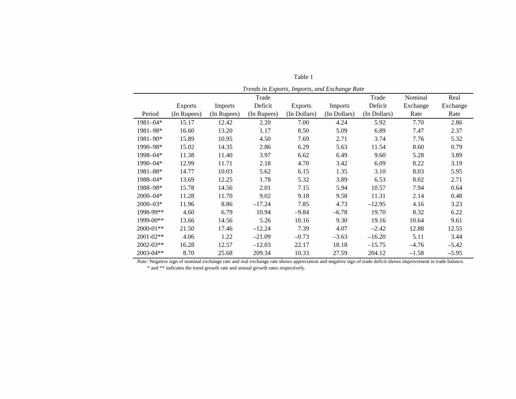
Table 1

Trends in Exports, Imports, and Exchange Rate

Period Exports

(In Rupees) Imports

(In Rupees)

Trade Deficit

(In Rupees) Exports

(In Dollars) Imports

(In Dollars)

Trade Deficit

(In Dollars)

Nominal Exchange

Rate

Real Exchange

Rate 1981–04* 15.17 12.42 2.20 7.00 4.24 5.92 7.70 2.86 1981–98* 16.60 13.20 1.17 8.50 5.09 6.89 7.47 2.37 1981–90* 15.89 10.95 4.50 7.69 2.71 3.74 7.76 5.32 1990–98* 15.02 14.35 2.86 6.29 5.63 11.54 8.60 0.79 1998–04* 11.38 11.40 3.97 6.62 6.49 9.60 5.28 3.89 1990–04* 12.99 11.71 2.18 4.70 3.42 6.09 8.22 3.19 1981–88* 14.77 10.03 5.62 6.15 1.35 3.10 8.03 5.95 1988–04* 13.69 12.25 1.78 5.32 3.89 6.53 8.02 2.71 1988–98* 15.78 14.56 2.01 7.15 5.94 10.57 7.94 0.64 2000–04* 11.28 11.70 9.02 9.18 9.58 11.31 2.14 0.48 2000–03* 11.96 8.86 –17.24 7.85 4.73 –12.95 4.16 3.23 1998-99** 4.60 6.79 10.94 –9.84 –6.78 19.70 8.32 6.22 1999-00** 13.66 14.56 5.26 10.16 9.30 19.16 10.64 9.61 2000-01** 21.50 17.46 –12.24 7.39 4.07 –2.42 12.88 12.55 2001-02** 4.06 1.22 –21.09 –0.73 –3.63 –16.20 5.11 3.44 2002-03** 16.28 12.57 –12.03 22.17 18.18 –15.75 –4.76 –5.42 2003-04** 8.70 25.68 209.34 10.33 27.59 204.12 –1.58 –5.95 Note: Negative sign of nominal exchange rate and real exchange rate shows appreciation and negative sign of trade deficit shows improvement in trade balance. * and ** indicates the trend growth rate and annual growth rates respectively.

Real Exchange Rate, Exports, and Imports Movements 187

balance. The rate of nominal devaluation was similar if we compare 1981–88 with 1988–98, however, the rate of real devaluation was higher in pre structural adjustment programme. Balance of trade situation worsened further in the post structural adjustment period; the rate of deterioration of trade balance which was 3.10 in the pre structural adjustment period increases to 10.57 percent (1988–98) in the post structural adjustment period. It is noted that in dollar terms the rate of deterioration in trade balance was higher in pre structural adjustment programme.

In July 1998, instead of adjusting the currency, the country moved to a dual exchange rate system (inter bank floating rate9 and composite rate).10 The dual exchange rate system was replaced by the unitary exchange rate system after one year in May 1999. Under this regime, the State Bank was able to intervene in the market for the sale and purchase of foreign exchange and authorised dealers were allowed to fix their own buying and selling rates subject to the condition that the difference between the two rates should not exceed Rs 0.50/$. In 1998 Pakistan had faced severe sanctions by international communities after the nuclear detonation. Pakistan was in deep trouble at that time because of having low level of reserves and our exports were not acceptable in many countries. During 1998-99 real devaluation was 6.22 percent and nominal devaluation was 8.30 percent. Exports grew by 4.60 percent, imports grew by 6.79 percent in rupee terms and declined in dollar terms and trade balance deteriorated in both rupee and dollar terms. The unitary exchange rate system was discontinued in July 2000 and replaced by the free float exchange rate regime. During 1999-00, real devaluation was 9.61 percent and nominal devaluation was 10.64 percent. Exports grew by 13.66 percent, imports grew by 14.56 percent, and the trade balance deteriorated by 19.16 percent. During 2000-2002 real exchange rate devalued at the rate of 3.16 percent and nominal devaluation was 4 percent, and during 2003-04 real exchange rate was appreciated by 5.95 percent and nominal exchange rate was appreciated by 1.58 percent. Under this regime, exports grew at 9.21 percent during 2000-2003, imports grew at 5.83 percent, and the trade balance improved by 11.68 percent. In the last year (2003–04) the growth rate of exports were recorded 10.33 percent while growth rate of imports was 27.59 percent. After 1997, it was the first time that in 2003–04 the trade deficit has exceeded 3 Billion dollars and put pressure on exchange rate to depreciate by 2.92 percent even in the presence of high inflow of foreign exchange reserves.

The above explanation shows that when the rate of real devaluation was lower there was a significant increase in the growth rate of imports; when the real devaluation was higher there was a significant increase in the growth rate of exports. This implies that there exists some kind of a long-run relationship between exports and real exchange rate and imports and real exchange rate. On the other hand, 96

9Determined by demand and supply of foreign exchange. 10Computed from a weighted average of the official and inter-bank floating rate.

Kemal and Qadir 188

percent correlation between imports and exports shows that there are strong long-run linkages between these two variables.

V. EMPIRICAL FINDINGS AND INTERPRETATION

OF THE RESULTS

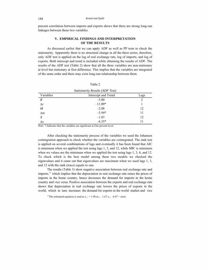
As discussed earlier that we can apply ADF as well as PP tests to check the stationarity. Apparently there is no structural change in all the three series, therefore, only ADF test is applied on the log of real exchange rate, log of imports, and log of exports. Both intercept and trend is included while obtaining the results of ADF. The results of the ADF test (Table 2) show that all the three variables are non-stationary at level but stationary at first difference. This implies that the variables are integrated of the same order and there may exist long-run relationship between them.

Table 2

Stationarity Results (ADF Test) Variables Intercept and Trend Lags R –3.00 2 ∆r –11.00* 1 M –2.08 12 ∆m –5.94* 11 X –1.83 12 ∆x –6.35* 11

Note: * Indicates that the variables are significant at One percent level.

After checking the stationarity process of the variables we used the Johansen

cointegration approach to check whether the variables are cointegrated. The rank test is applied on several combinations of lags and eventually it has been found that AIC is minimum when we applied the test using lags 1, 3, and 12, while SBC is minimum when we values are the minimum when we applied the test using lags 1, 3, 6, and 12. To check which is the best model among these two models we checked the eigenvalues and it came out that eigenvalues are maximum when we used lags 1, 3, and 12 with the rank (trace) equals to one.

The results (Table 3) show negative association between real exchange rate and imports,11 which implies that the depreciation in real exchange rate raises the prices of imports in the home country, hence decreases the demand for imports in the home country and vice versa. Positive association between the exports and real exchange rate shows that depreciation in real exchange rate lowers the prices of exports in the world, which in turn increases the demand for exports in the world market and vice

11The estimated equation is read as rt–1 + 1.98 mt–1 –1.67 xt–1 –6.07 = error.

Real Exchange Rate, Exports, and Imports Movements 189

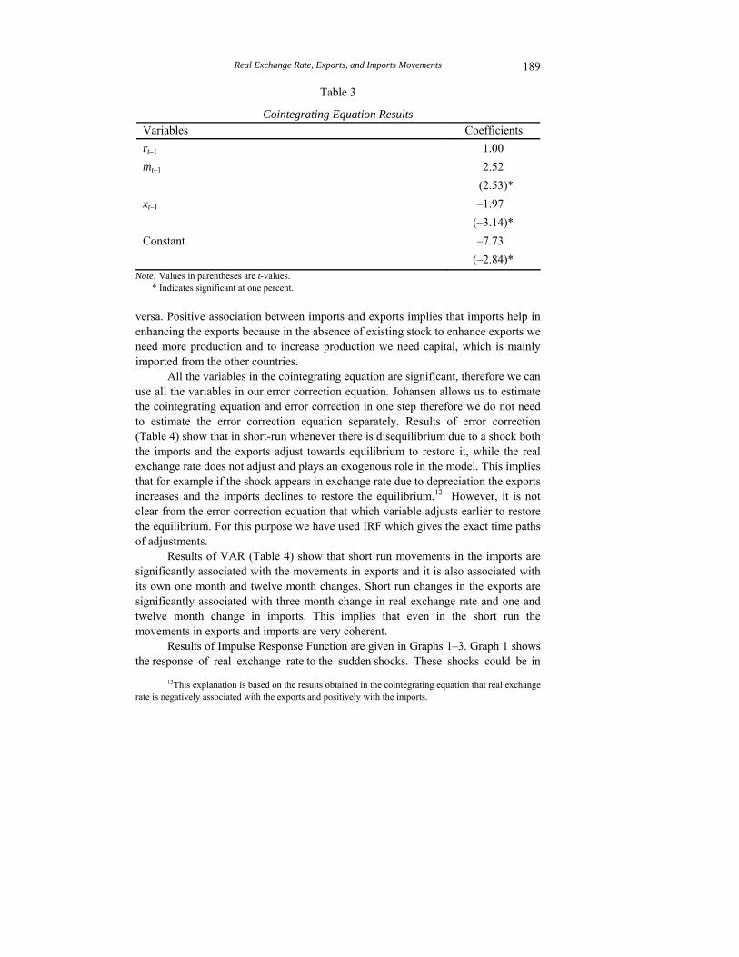
Table 3

Cointegrating Equation Results Variables Coefficients rt–1 1.00 mt–1 2.52 (2.53)* xt–1 –1.97 (–3.14)* Constant –7.73 (–2.84)*

Note: Values in parentheses are t-values. * Indicates significant at one percent. versa. Positive association between imports and exports implies that imports help in enhancing the exports because in the absence of existing stock to enhance exports we need more production and to increase production we need capital, which is mainly imported from the other countries.

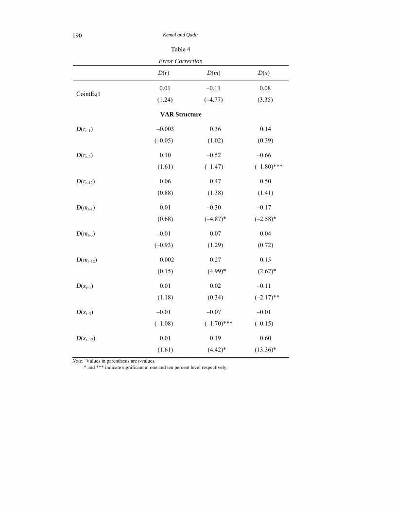
All the variables in the cointegrating equation are significant, therefore we can use all the variables in our error correction equation. Johansen allows us to estimate the cointegrating equation and error correction in one step therefore we do not need to estimate the error correction equation separately. Results of error correction (Table 4) show that in short-run whenever there is disequilibrium due to a shock both the imports and the exports adjust towards equilibrium to restore it, while the real exchange rate does not adjust and plays an exogenous role in the model. This implies that for example if the shock appears in exchange rate due to depreciation the exports increases and the imports declines to restore the equilibrium.12 However, it is not clear from the error correction equation that which variable adjusts earlier to restore the equilibrium. For this purpose we have used IRF which gives the exact time paths of adjustments.

Results of VAR (Table 4) show that short run movements in the imports are significantly associated with the movements in exports and it is also associated with its own one month and twelve month changes. Short run changes in the exports are significantly associated with three month change in real exchange rate and one and twelve month change in imports. This implies that even in the short run the movements in exports and imports are very coherent.

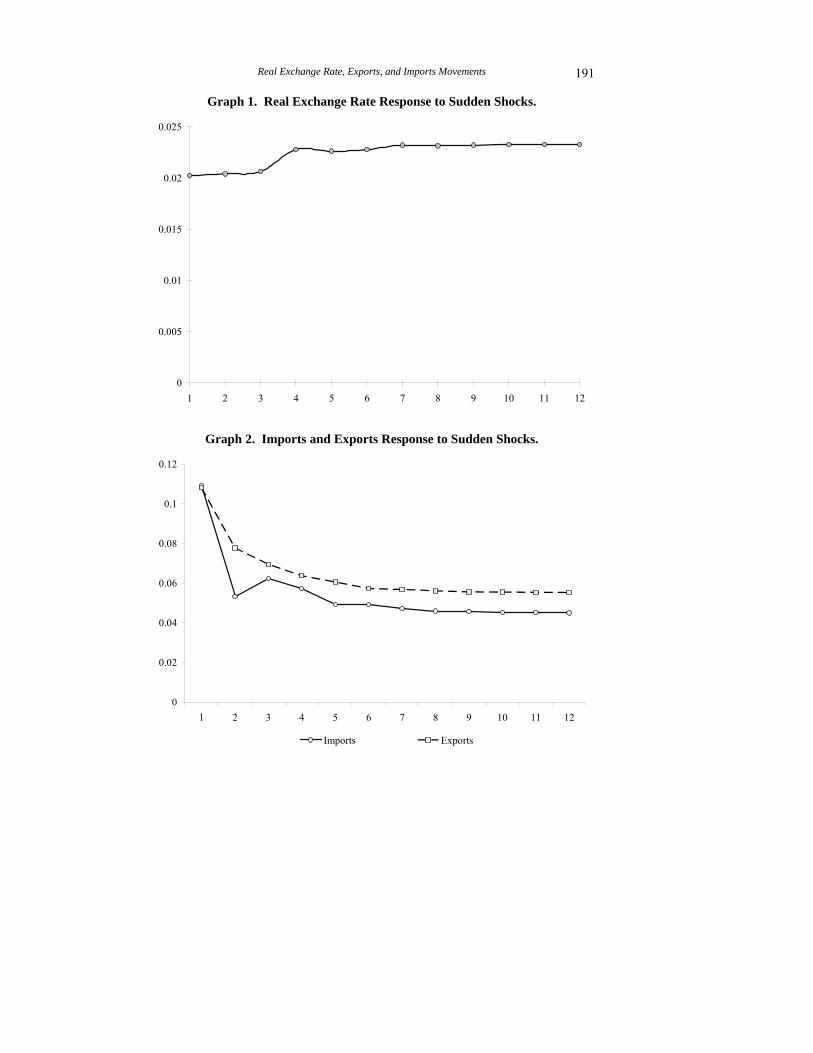
Results of Impulse Response Function are given in Graphs 1–3. Graph 1 shows the response of real exchange rate to the sudden shocks. These shocks could be in

12This explanation is based on the results obtained in the cointegrating equation that real exchange rate is negatively associated with the exports and positively with the imports.

Kemal and Qadir 190

Table 4

Error Correction

D(r) D(m) D(x)

CointEq1 0.01

(1.24)

–0.11

(–4.77)

0.08

(3.35)

VAR Structure

D(rt–1) –0.003

(–0.05)

0.36

(1.02)

0.14

(0.39)

D(rt–3) 0.10

(1.61)

–0.52

(–1.47)

–0.66

(–1.80)***

D(rt–12) 0.06

(0.88)

0.47

(1.38)

0.50

(1.41)

D(mt–1) 0.01

(0.68)

–0.30

(–4.87)*

–0.17

(–2.58)*

D(mt–3) –0.01

(–0.93)

0.07

(1.29)

0.04

(0.72)

D(mt–12) 0.002

(0.15)

0.27

(4.99)*

0.15

(2.67)*

D(xt–1) 0.01

(1.18)

0.02

(0.34)

–0.11

(–2.17)**

D(xt–3) –0.01

(–1.08)

–0.07

(–1.70)***

–0.01

(–0.15)

D(xt–12) 0.01

(1.61)

0.19

(4.42)*

0.60

(13.36)*

Note: Values in parenthesis are t-values. * and *** indicate significant at one and ten percent level respectively.

Real Exchange Rate, Exports, and Imports Movements 191

Graph 1. Real Exchange Rate Response to Sudden Shocks.

0

0.005

0.01

0.015

0.02

0.025

1 2 3 4 5 6 7 8 9 10 11 12

Graph 2. Imports and Exports Response to Sudden Shocks.

0

0.02

0.04

0.06

0.08

0.1

0.12

1 2 3 4 5 6 7 8 9 10 11 12

Imports Exports

Kemal and Qadir 192

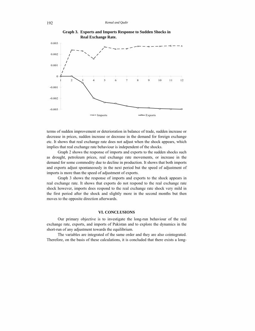
Graph 3. Exports and Imports Response to Sudden Shocks in Real Exchange Rate.

-0.003

-0.002

-0.001

0

0.001

0.002

0.003

1 2 3 4 5 6 7 8 9 10 11 12

Imports Exports terms of sudden improvement or deterioration in balance of trade, sudden increase or decrease in prices, sudden increase or decrease in the demand for foreign exchange etc. It shows that real exchange rate does not adjust when the shock appears, which implies that real exchange rate behaviour is independent of the shocks.

Graph 2 shows the response of imports and exports to the sudden shocks such as drought, petroleum prices, real exchange rate movements, or increase in the demand for some commodity due to decline in production. It shows that both imports and exports adjust spontaneously in the next period but the speed of adjustment of imports is more than the speed of adjustment of exports.

Graph 3 shows the response of imports and exports to the shock appears in real exchange rate. It shows that exports do not respond to the real exchange rate shock however, imports does respond to the real exchange rate shock very mild in the first period after the shock and slightly more in the second months but then moves to the opposite direction afterwards.

VI. CONCLUSIONS

Our primary objective is to investigate the long-run behaviour of the real exchange rate, exports, and imports of Pakistan and to explore the dynamics in the short-run of any adjustment towards the equilibrium.

The variables are integrated of the same order and they are also cointegrated. Therefore, on the basis of these calculations, it is concluded that there exists a long-

Real Exchange Rate, Exports, and Imports Movements 193

run relationship between the real exchange rate, exports, and imports. It is also concluded that the real exchange rate is negatively associated with the exports and positively associated with the imports. This implies that devaluation might be helpful in improving the trade balance.

In short-run imports and exports adjust towards their equilibrium when there is disequilibrium. The adjustment in imports is spontaneous; it starts adjusting in the next period soon after the appearing of the shock. Similarly, adjustment in exports is spontaneous as well, and it starts adjusting in the next period soon after the appearing of the shock. However, adjustment in the imports is greater than the adjustment in the exports. The exports do not respond to the shock caused by the real exchange rate. This implies that exporters are the least bothered by the shocks in the real exchange rate. They only need to have more orders (consignments) and if the orders are sufficient shocks in exchange rate does not have any impact on exports. Imports respond to the sudden shock in the real exchange rate. This implies that importers have fear of excessive appreciation and depreciation, which they want to avoid.

Good news for the government that the sudden movements in the real exchange rate do not affect exports, therefore, Pakistan should not worry of exchange rate shocks. However, after September 11, 2001 the rupee has gained strength because of high inflow of foreign exchange and remittances and higher value of rupee will compete out Pakistani exports. But it is observed that this is not the case in the last four years. In a survey13 of various industrialists, it has been found that exporters do not want to export at the appreciated exchange rate in the market. However, they are still exporting because they have found new markets and they do not want to lose their old markets. This leads us to the conclusion that to enhance exports, we must explore more markets through international trade fairs and Commercial Attaché positions in the other countries.

REFERENCES

Alexander, Sidney S. (1952) The Effects of Devaluation on a Trade Balance. IMF Staff Papers 2 (April), 263–278.

Bahmani-Oskooee, M. (1985) Devaluation and the J-Curve: Some Evidence from LDCs. The Review of Economics and Statistics (August), 500–504.

Bahmani-Oskooee, M. (1994) Are Imports and Exports of Australia Cointegrated. Journal of Economic Integration 9, 525–533.

Connolly, M., and Dean Taylor (1972) Devaluation in Less Developed Countries. Prepared for a conference on Devaluation sponsored by the Board of Governors, Federal Reserve System, Washington, D. C., December 14-15.

13The survey on “Trade Export Promotion and Industry” was conducted by the Pakistan Institute

of Development Economics in March-April 2002 and was sponsored by Asian Development Bank.

Kemal and Qadir 194

Cooper, Richard N. (1971) An Assessment of Currency Devaluation in Developing Countries. In Gustav Ranis (ed.) Government and Economic Development. New Haven, Conn.: Yale University Press (for Yale University, Economic Growth Centre).

Cooper, Richard N. (1971a) Currency Devaluation in Developing Countries. Essays in International Finance, No. 86. Princeton University, International Finance Section.

Dornbusch, R. (1973) Devaluation, Money and Non-traded Goods. American Economic Review 63:5 (December), 871–80.

Ender, Walter (1995) Applied Econometric Time Series. Canada: John Willey & Sons.

Engle, Robert F., and C. W. J. Granger (1987) Cointegration and Error Corrrection: Representation, Estimation and Testing. Econometrica 55, 251–276.

Frenkel, Jacob A., and Carlos Rodriguez (1975) Portfolio Equilibrium and the Balance of Payments: A Monetary Approach. American Economic Review 65:4, 143–59.

Himarios, Daniel (1989) Do Devaluations Improve the Trade Balance? The Evidence Revisited. Economic Inquiry (January), 143–168.

Husted, S. (1992) The Emerging U. S. Current Account Deficit in the 1980’s: A Cointegration Analysis. Review of Economics and Statistics 74, 159–166.

International Monetary Fund (Various Issues) International Financial Statistics. Washington, D. C.: IMF.

Johansen, S., and K. Juselius (1990) The Maximum Likelihood Estimation and Inference on Cointegration—With Application to Demand for Money. Oxford Bulletin of Economics and Statistics 52, 169–210.

Johnson, Harry G. (1967) Towards a General Theory of the Balance of Payments. In International Trade and Economic Growth: Studies in Pure Theory. Cambridge, Mass.: Harvard University Press.

Junz, M., and Rudolph R. Rhomberg (1973) Price Competitiveness in Export Trade among Industrial Countries. American Economic Review, Papers and Proceedings 63 (May), 412–418.

Khan, Farzana Naheed (1999) Real Exchange Rate Movements and Purchasing Power Parity: The Asian Experience. (M.Phil Thesis, Quaid-i-Azam Univetrsity).

Laffer, Arthur B. (1976) Exchange Rates, the Terms of Trade and the Trade Balance. In Effects of Exchange Rate Adjustments. Washington, D. C.: Treasury Dept., OASIA Res.

Maddala, G. S., and I. M. Kim (1998) Unit Roots, Cointegration, and Structural Change. Cambridge University Press.

Magee, Stephen P. (1973) Currency Contracts, Pass Through and Devaluation. Brookings Papers on Economic Activity 1, 303–325.

Real Exchange Rate, Exports, and Imports Movements 195

Metzler, Lloyd (1948) The Theory of International Trade. In Howard S. Ellis (ed.) A Survey of Contemporary Economics. Vol. I. Philadelphia: Blakiston.

Mundell, Robert A. (1971) Monetary Theory: Inflation, Interest, and Growth in the World Economy. Pacific Palisades, Calif.: Goodyear.

Ng, S., and P. Perron (1995) Unit Root Tests in ARMA Models with Data—Dependent Methods for the Selection of the Truncation Lag. Journal of American Statistical Association 90, 268–81.

Paleologos, John M., and Spyros E. Georgantelis (1997) Exchange Rate Movements and the Trade Balance Deficit: A Multivariate Analysis. Economia Internazionale 3 (August), 459–474.

Robinson, Joan (1947) The Foreign Exchanges. In Essays in the Theory of Employment. Oxford: Blackwell.

Salant, Michael (1976) Devaluations Improve the Balance of Payments Even if Not the Trade Balance. In Effects of Exchange Rate Adjustments. Washington, D. C.: Treasury Dept., OASIA Res.

Trade Export Promotion and Industry (TEPI) (2002) Project financed by Asian Development Bank, Conducted by Pakistan Institute of Development Economics.

Upadhayaya, Kamal P., Franklin G. Mixon, Jr., and Dharmendra Dhakal (1998) “Do Devaluations Improve Trade Balances? Evidence from Four South Asian Countries. Indian Economic Journal 46:3 (January-March), 91–97.

Williamson, J. (1983) The Open Economy and the World Economy. Basic Books Inc.