Reaction-Diffusion - Traveling Waves in Oregonator Model of Belousov-Zhabotinsky Reaction Richard K. Herz, [email protected], April 2015 Below are results of numerical simulations showing traveling waves in the Oregonator model. A simple finite difference method was used to solve the system of partial differential equations (PDE) in order to illustrate basic principles. For a one dimensional spatial field, the equations are in the form, ∂ C i ∂ t = D i ∂ 2 C i ∂ x 2 + r i For explanations, see www.ReactorLab.net, Math Tools, MATLAB examples, the last three rows. The notes on that page for integration of PDEs are attached to this document for convenience. Once you understand the principles, you can use the pdepe function in MATLAB, or a finite element tool such as COMSOL for more complex examples. In this simulation, bromous acid and bromide ion diffuse. The cerium redox catalyst does not diffuse: it is coated over a surface or impregnated in a membrane which contact the liquid reactants. Below, a wave is initiated on the left side of the field. Zero-flux boundary conditions are specified on both sides. Time proceeds down the image. You can see a sequence of waves propagating from left to right. 1 of 7

Welcome message from author
This document is posted to help you gain knowledge. Please leave a comment to let me know what you think about it! Share it to your friends and learn new things together.
Transcript

Reaction-Diffusion - Traveling Waves in Oregonator Model of Belousov-Zhabotinsky Reaction
Richard K. Herz, [email protected], April 2015
Below are results of numerical simulations showing traveling waves in the Oregonator model. A simplefinite difference method was used to solve the system of partial differential equations (PDE) in order to illustrate basic principles. For a one dimensional spatial field, the equations are in the form,
∂Ci
∂ t=D
i
∂2C
i
∂ x2 +r
i
For explanations, see www.ReactorLab.net, Math Tools, MATLAB examples, the last three rows. The notes on that page for integration of PDEs are attached to this document for convenience. Once you understand the principles, you can use the pdepe function in MATLAB, or a finite element tool such as COMSOL for more complex examples.
In this simulation, bromous acid and bromide ion diffuse. The cerium redox catalyst does not diffuse: itis coated over a surface or impregnated in a membrane which contact the liquid reactants. Below, a wave is initiated on the left side of the field. Zero-flux boundary conditions are specified on both sides. Time proceeds down the image. You can see a sequence of waves propagating from left to right.
1 of 7

Here is a plot of the HBrO2 signal across the 1D field, with lines at different times. This is another way to see the wave propagating from left to right.
Waves and 2D patterns require that the activator (HBrO2 here) and inhibitor (Ce(IV) here) have different diffusion coeffient values. The boundary conditions and coarse grid used in this simulation arenot the best case for investigating this effect. Below we have run the simulation above after changing the diffusion coefficient for Ce(IV) from zero to the same value as for HBrO2. The traveling waves do not appear now. Instead, the entire 1D field oscillates at the same time.
R. K. Herz, [email protected], p. 2 of 7
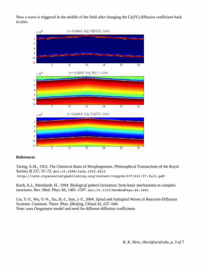
Now a wave is triggered in the middle of the field after changing the Ce(IV) diffusion coefficient back to zero.
References
Turing, A.M., 1952. The Chemical Basis of Morphogenesis. Philosophical Transactions of the Royal Society B 237, 37–72. doi:10.1098/rstb.1952.0012 http://rstb.royalsocietypublishing.org/content/royptb/237/641/37.full.pdf
Koch, A.J., Meinhardt, H., 1994. Biological pattern formation: from basic mechanisms to complex structures. Rev. Mod. Phys. 66, 1481–1507. doi:10.1103/RevModPhys.66.1481
Liu, Y.-F., Wu, Y.-N., Xu, H.-J., Sun, J.-F., 2004. Spiral and Antispiral Waves in Reaction-Diffusion Systems. Commun. Theor. Phys. (Beijing, China) 42, 637–640. Note: uses Oregonator model and need for different diffusion coefficients
R. K. Herz, [email protected], p. 3 of 7

Listing of Matlab script
% 1D waves in scaled Oregonator model of BZ reaction% Here write a finite difference method% Alternatively use Matlab function pdepe or COMSOL (finite element)% Use scaled rate equations from this link% http://www.scholarpedia.org/article/Oregonator
clear allclose allfprintf('--------------------------------- \n') % run separator
% x = HBrO2% y = Br(-)% z = Ce(IV)
% see oregonatorParams.m for paramsinve = 1.01010101010101e+02;invep = 5.05050505050505e+04;qp = 7.69696969696970e-03;qpp = 3.84848484848485e+00;fp = 5.05050505050505e+04;
% diffusion coefficientDx = 0.2e-5; % HBrO2Dy = Dx; % Br(-)Dz = 0; % Ce(IV)/Ce(III) doesn't diffuse in this example% example is cerium impregnated membrane in which other components diffuse
% set up finite difference grid% tdiv must vary with sdiv for numerical stability% tdiv >= 10*sdiv^2sdiv = 30; % number spatial divisionstfinal = 12; % final time
dt = 1e-5; % time step needed for Euler integration of ODEs = 1e-5% check criterion for numerical stability % see notes, the one here may not be the besttdiv = round(tfinal/dt);if tdiv < 10*sdiv^2 fprintf('WARNING: decrease dt or sdiv for stability \n')endlen = 0.1; % length of field, use len since length is reserved
ds = len/sdiv;ds2 = ds^2; % do once here to save time in repeat
% initial conditions from ode45 run% just before a "pulse"% x0 = 3.3266e-4; % HBrO2% y0 = 0.06619; % Br(-)% z0 = 3.5645e-4; % Ce(IV)
% set initial conditions with Ce(IV) high% such that onset of oscillations is suppressedx = 3.3266e-4 * ones(tdiv+1, sdiv+1); % HBrO2y = 0.06619 * ones(tdiv+1, sdiv+1); % Br(-)z = 4 * 3.5645e-4 * ones(tdiv+1, sdiv+1); % Ce(IV)
R. K. Herz, [email protected], p. 4 of 7

% TRIGGER WAVE by lowering Ce(IV) to critical value at one node% z(1, round(sdiv/2)) = 0.8905*z(1,1); % <<<< ACTIVATE THIS LINE, CENTERz(1,1) = 0.8905 *z(1,1); % <<<< ACTIVATE THIS LINE, LEFT SIDE
% boundary conditions and coarse grid here not best to investigate% effect of diffusion coefficients on presence or absence of waves% near center, wave at 0.8905 & no wave at Dz=Dx% near center, no wave >= 0.891 but still get wave at 0.890 & Dz=Dx% left side, wave at 0.8905 & no wave at Dz=Dx% left side, no wave >= 0.892, no wave 0.891 with Dz=Dx, wave 0.890 Dz=Dx
for j = 1:tdiv % step in time
% first do both boundary conditions at s = 0 & s = len (length) % use zero-flux BC at both boundaries, d2y/ds2 = 0, etc.
i = 1; % at s = 0
% compute local rates rx = qp*y(j,i) - inve*x(j,i)*y(j,i) + inve*x(j,i)*(1 - x(j,i)); ry = -qpp*y(j,i) - invep*x(j,i)*y(j,i) + fp*z(j,i); rz = x(j,i) - z(j,i);
dxdt = Dx*((2*x(j,i+1) - 2*x(j,i))/ds2) + rx; dydt = Dy*((2*y(j,i+1) - 2*y(j,i))/ds2) + ry; dzdt = Dz*((2*z(j,i+1) - 2*z(j,i))/ds2) + rz;
x(j+1,i) = x(j,i) + dxdt * dt; y(j+1,i) = y(j,i) + dydt * dt; z(j+1,i) = z(j,i) + dzdt * dt;
i = sdiv+1; % at s = len (length)
% compute local rates rx = qp*y(j,i) - inve*x(j,i)*y(j,i) + inve*x(j,i)*(1 - x(j,i)); ry = -qpp*y(j,i) - invep*x(j,i)*y(j,i) + fp*z(j,i); rz = x(j,i) - z(j,i);
% note change to 2*x(j,i-1) from 2*x(j,i+1) for s = 0 above dxdt = Dx*((2*x(j,i-1) - 2*x(j,i))/ds2) + rx; dydt = Dy*((2*y(j,i-1) - 2*y(j,i))/ds2) + ry; dzdt = Dz*((2*z(j,i-1) - 2*z(j,i))/ds2) + rz;
x(j+1,i) = x(j,i) + dxdt * dt; y(j+1,i) = y(j,i) + dydt * dt; z(j+1,i) = z(j,i) + dzdt * dt;
% now do interior spatial nodes
for i = 2:sdiv
% compute local rates rx = qp*y(j,i) - inve*x(j,i)*y(j,i) + inve*x(j,i)*(1 - x(j,i)); ry = -qpp*y(j,i) - invep*x(j,i)*y(j,i) + fp*z(j,i); rz = x(j,i) - z(j,i);
R. K. Herz, [email protected], p. 5 of 7

dxdt = Dx*((x(j,i+1)-2*x(j,i)+x(j,i-1))/ds2) + rx; dydt = Dy*((y(j,i+1)-2*y(j,i)+y(j,i-1))/ds2) + ry; dzdt = Dz*((z(j,i+1)-2*z(j,i)+z(j,i-1))/ds2) + rz;
x(j+1,i) = x(j,i) + dxdt * dt; y(j+1,i) = y(j,i) + dydt * dt; z(j+1,i) = z(j,i) + dzdt * dt;
endend
%% plot results
% put plotting in separate% "code sections" starting with %%% so can change plots% by clicking "Run Section" in Editor% without having to redo integraton
colormap(jet(255))logx = log10(x);logy = log10(y);logz = log10(z);maxLogX = max(max(logx));maxLogY = max(max(logy));maxLogZ = max(max(logz));minLogX = min(min(logx));minLogY = min(min(logy));minLogZ = min(min(logz));logx = 255 * (logx-minLogX)/(maxLogX-minLogX);logy = 255 * (logy-minLogY)/(maxLogY-minLogY);logz = 255 * (logz-minLogZ)/(maxLogZ-minLogZ);
subplot(3,1,1), image(logx), title('x = scaled log HBrO2 conc','FontSize',14)subplot(3,1,2), image(logy), title('y = scaled log Br(-) conc','FontSize',14)subplot(3,1,3), image(logz), title('z = scaled log Ce(IV) conc','FontSize',14)
%% plot wave
% plot wave across field% stepping in time
% wait for multiple sets of waves
% here plot logx (HBrO2)
figure(2)plot(logx(1,:),'r')axis([0 35 0 300]) % here for sdiv = 30 & color scaled to 255title('Oregonator Waves - scaled log HBrO2','FontSize',14)hold onpp = 0.1;pause(pp)plot(logx(1,:),'w') % erase last line [rows cols] = size(logx);nf = 5000;
R. K. Herz, [email protected], p. 6 of 7

jmax = round(rows/nf);for j = 2:jmax % wait for multiple sets of waves plot(logx(1+j*nf,:),'r') pause(pp) plot(logx(1+j*nf,:),'w') % erase last lineendplot(logx(1+j*nf,:),'r')hold off
Listing of file oregonatorParams.m to compute parameter values
% params for oregonator model% http://www.scholarpedia.org/article/Oregonator% use scaled equations from this link% calculate params here to save time in repeats
A = 0.06;B = 0.02;q = 7.62e-5;e = 9.90e-3;ep = 1.98e-5;f = 1;
format long e
inve = 1/einvep = 1/epqp = inve*qqpp = invep*qfp = invep*f
% results copied to script% inve = 1.01010101010101e+02;% invep = 5.05050505050505e+04;% qp = 7.69696969696970e-03;% qpp = 3.84848484848485e+00;% fp = 5.05050505050505e+04;
CHECK FOR FOLLOWING PAGES >>>>
R. K. Herz, [email protected], p. 7 of 7

Numerical Integration of Differential Equations, PART Bby Richard K. Herz <[email protected]>
Finite Difference Method for Integration of PDE’s
These notes will consider integration of the following parabolic PDE using the finite difference method.
∂c∂t
= D∂2c
∂x2
Note that this mass diffusion equation has an analogous form for heat conduction, with temperature, T, replacing concentration, c, and thermal diffusivity, α = kt / ρCp, replacing the mass diffusivity D.
Since there is variation with time we need an initial condition and since there is a second derivative with respect to position we need two boundary conditions.
Initial Condition: c(x,0) = K1Boundary condition at x = 0, c(0,t) = K2Boundary condition at x = xmax
∂c∂x x = xmax
= 0
Imagine that spatial position x and time t are represented by a grid, with each node of the grid representing a point in x and a point in time. The spacing of the nodes along the x direction is ∆x and the spacing of the nodes along the t direction is ∆t. We use the subscript i to indicate which x location we are at and the superscript j to indicate which t location we are at on the grid.
x x = xmaxx = 0
i = 0 i = m
j = 0
j = 5
t
node i = 3, j = 2 hasconcentration value
c j
i= c2
3

The first derivative of c with respect to x is approximated by the “finite difference” approximation
∂c∂x ≈
ci + 1 – ci
Δx
The second derivative of c with respect to x is approximated by the following “centered finite difference derivative”:
∂2c
∂x2≈ lim
Δx → 0
∂c∂x i + 1
–∂c∂x i
Δx≈
ci + 1 – ci
Δx–
ci – ci – 1
ΔxΔx
∂2c
∂x2≈
ci + 1 – 2 ci + ci – 1
Δx2
The time derivative is approximated by the following “forward finite divided difference” which is equivalent to using Euler’s method to integrate in time:
∂c∂t
≈ci
j + 1– ci
j
Δt
The finite difference approximation to our PDE is:
ci
j + 1– ci
j
Δt= D
ci + 1
j– 2 ci
j+ ci – 1
j
Δx 2
Rearranging, we have the result for the concentration c at the next time step, j+1, as a function of concentrations at the current time step j:
ci
j + 1= ci
j+ λ ci + 1
j– 2 ci
j+ ci – 1
j
λ =D Δt
Δx 2
The above equation can be applied at all the internal nodes, that is, all nodes except those at the boundaries: node i = 0 representing position x = 0 and node i = m representing x = xmax.
At x = 0, the boundary condition above specifies that c0 equals the constant K2.
At x = xmax, the boundary condition above is the “zero flux” boundary condition. This type of
boundary condition is also encountered at planes of symmetry:

i = m
x = xmax
conc
x
plane of symmetry orimpermeable surface
dc/dx = 0
We can formulate the difference equation for the node at i = m, x = xmax, by referencing an imaginary
node at an imaginary grid location i = m + 1, where this imaginary node has the same concentration c as the node at i = m – 1. This would be the case for a concentration profile that is symmetrical about the plane at x = xmax, i = m.
i = 0 i = m
j = 0
j = 5
t
x
i = m+1
imaginary node
these two nodeshave the same concentrationfor a zero-flux boundary condition(symmetry condition) at i = m
x = xmaxx = 0
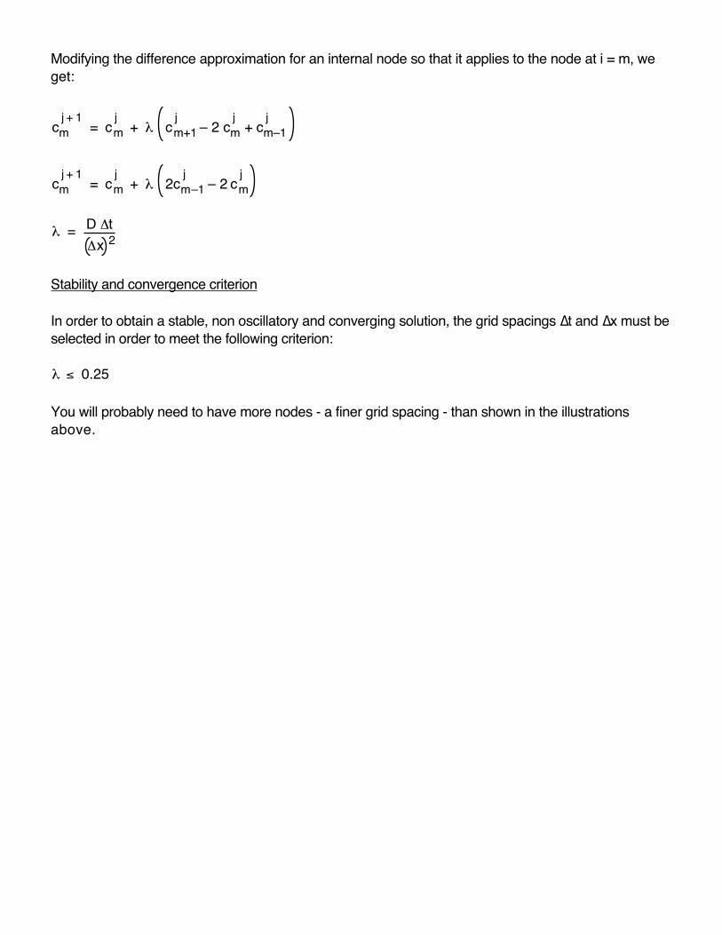
Modifying the difference approximation for an internal node so that it applies to the node at i = m, we
get:
cm
j + 1= cm
j+ λ cm+1
j– 2 cm
j+ cm–1
j
cm
j + 1= cm
j+ λ 2cm–1
j– 2 cm
j
λ =D Δt
Δx 2
Stability and convergence criterion
In order to obtain a stable, non oscillatory and converging solution, the grid spacings ∆t and ∆x must be
selected in order to meet the following criterion:
λ ≤ 0.25
You will probably need to have more nodes - a finer grid spacing - than shown in the illustrations
above.
Related Documents