1 Re-localisation of Microscopic Lesions in their Macroscopic Context for Surgical Instrument Guidance Baptiste Allain A dissertation submitted for the degree of Doctor of Philosophy of the University College London - UCL Centre for Medical Image Computing - CMIC Department of Medical Physics and Bioengineering University College London Submitted in July 2011

Welcome message from author
This document is posted to help you gain knowledge. Please leave a comment to let me know what you think about it! Share it to your friends and learn new things together.
Transcript

1
Re-localisation of Microscopic Lesions in their
Macroscopic Context for Surgical Instrument
Guidance
Baptiste Allain
A dissertation submitted for the degree of
Doctor of Philosophy
of the
University College London - UCL
Centre for Medical Image Computing - CMIC
Department of Medical Physics and Bioengineering
University College London
Submitted in July 2011

2
I, Baptiste Allain, confirm that the work presented in this thesis is my own. Where
information has been derived from other sources, I confirm that this has been indicated in the
thesis.
3
Abstract Optical biopsies interrogate microscopic structure in vivo with a 2mm diameter miniprobe
placed in contact with the tissue for detection of lesions and assessment of disease
progression. After detection, instruments are guided to the lesion location for a new optical
interrogation, or for treatment, or for tissue excision during the same or a future examination.
As the optical measurement can be considered as a point source of information at the surface
of the tissue of interest, accurate guidance can be difficult. A method for re-localisation of the
sampling point is, therefore, needed.
The method presented in this thesis has been developed for biopsy site re-localisation
during a surveillance examination of Barrett’s Oesophagus. The biopsy site, invisible
macroscopically during conventional endoscopy, is re-localised in the target endoscopic
image using epipolar lines derived from its locations given by the tip of the miniprobe visible
in a series of reference endoscopic images. A confidence region can be drawn around the re-
localised biopsy site from its uncertainty that is derived analytically. This thesis also presents
a method to improve the accuracy of the epipolar lines derived for the biopsy site re-
localisation using an electromagnetic tracking system.
Simulations and tests on patient data identified the cases when the analytical
uncertainty is a good approximation of the confidence region and showed that biopsy sites
can be re-localised with accuracies better than 1mm. Studies on phantom and on porcine
excised tissue demonstrated that an electromagnetic tracking system contributes to more
accurate epipolar lines and re-localised biopsy sites for an endoscope displacement greater
than 5mm. The re-localisation method can be applied to images acquired during different
endoscopic examinations. It may also be useful for pulmonary applications. Finally, it can be
combined with a Magnetic Resonance scanner which can steer cells to the biopsy site for
tissue treatment.

4
The patient data collection was undertaken with the ethical approval 08/H0808/08 in the
Department of Gastroenterology of University College London Hospitals, UCLH NHS.

5
Acknowledgements I would like to thank my supervisors and employers Dr. Richard J. Cook, Dr. Mingxing Hu,
and Professor David J. Hawkes. They welcomed me in the department of Biomaterials,
Dental Institute, King’s College London, and in the Centre for Medical Image Computing,
University College London. They encouraged and guided me, but they also helped me find
my own solutions and make contributions. They put a lot of effort to correct and to suggest
improvements to my publications and my thesis. I am grateful to Dr. Richard Cook who
provided me with my salary through the Department of Health, UK, in order to accomplish
my work and my thesis and who gave me full access to his Fibered Confocal Microscope
(Cellvizio®, Mauna Kea Technologies, Paris, France).
My acknowledgements go as well to Dr. Tom Vercauteren who helped me find the
clinical application of the surveillance examination of Barrett’s Oesophagus and who
participated actively to the corrections of the publications, to Dr. Laurence Lovat who gave
me the patient data that he acquired during the surveillance examinations of Barrett’s
Oesophagus, and to Dr. Frederic Festy and Julien Festy who assisted me for the preparation
of the experiments on phantom and on excised organs of pigs and who gave me access to
their optics lab in the department of Biomaterials, Dental Institute, King’s College London.
I had also the chance to do some collaborative work with Johannes Riegler, Manfred
Junemann Ramirez, Dr. Anthony Price, and Dr. Mark Lythgoe. I would like to thank them for
providing me with tissue samples and cells in order to perform microscopic observations with
the Fibered Confocal Microscope or for giving me access to the 9.4T MR scanner at the
Centre for Advanced Biomedical Imaging, University College London. Our collaborative
work resulted in common publications.
I would like to thank all of my colleagues at the Centre for Medical Image
Computing, especially Yipeng Hu, Daniel Heanes, and Dr. Xiahai Zhuang, who were open to
discussions and who helped me at any stage of my project.
Finally, I would like to thank my family Professor Hervé Allain, Nicole Allain,
Pierre-Yves Allain, Bertrand and Jae-Hyun Allain, Solene and Adriano Zammito, my dear
Katy Ordidge as well as my friends, in particular Yvan and Lorraine Wibaux, Mathieu
Lemaire, Caroline Rodier, Jamie Brothwell, Tom MacDermott, Maria Antonia Gabarro
Aurell, and Lehna Hewitt for their encouragements over the last three years.

6
Table of contents
ABSTRACT.............................................................................................................................................3
ACKNOWLEDGEMENTS .....................................................................................................................5
TABLE OF CONTENTS.........................................................................................................................6
LIST OF FIGURES................................................................................................................................12
LIST OF TABLES .................................................................................................................................25
NOMENCLATURE AND ABBREVIATIONS ....................................................................................26
CHAPTER 1 INTRODUCTION: THE NEED FOR ACCURATE RE-LOCALISATION OF
MICROSCOPIC LESIONS IN THEIR MACROSCOPIC CONTEXT AFTER DETECTION BY
OPTICAL BIOPSY................................................................................................................................29
1.1 INTRODUCTION.............................................................................................................................29
1.2 BACKGROUND: DETECTION OF LESIONS STARTING AT THE SUPERFICIAL LAYERS OF TISSUE BY
OPTICAL BIOPSY .................................................................................................................................29 1.2.1 Development of cancers ......................................................................................................30 1.2.2 In vivo and in situ detection of lesions by optical biopsy ....................................................31
1.3 EXAMPLES OF INFORMATION EXTRACTED BY OPTICAL BIOPSY.....................................................32 1.3.1 Optical biopsy for the study of the spectrum of light after interaction with the tissue ........32 1.3.2 Optical biopsy for the study of the morphology of the cells................................................32 1.3.3 Detection of lesions based on functional imaging ...............................................................34
1.4 MOTIVATION ................................................................................................................................36 1.4.1 Extensions of the field of view of microscopic images .......................................................36 1.4.2 Need for accurate re-localisation of microscopic lesions detected by optical biopsy in the
macroscopic space of the organ of interest ...................................................................................37
1.5 STATEMENT OF CONTRIBUTION ....................................................................................................38
1.6 STRUCTURE OF THE THESIS...........................................................................................................39
CHAPTER 2 INITIAL PILOT WORK TO ASSESS THE IN VIVO USE OF THE FIBERED
CONFOCAL MICROSCOPE AND ITS USE IN COMBINATION WITH MRI.................................43

7 2.1 INTRODUCTION.............................................................................................................................43
2.2 FIBERED CONFOCAL MICROSCOPY...............................................................................................43 2.2.1 Confocal microscopy ...........................................................................................................43 2.2.2 Fibered confocal microscopy...............................................................................................45 2.2.3 Experiment: Level of details reached by the fibered confocal microscope .........................46
2.2.3.1 Materials and method...................................................................................................................46 2.2.3.2 Results and discussion .................................................................................................................47
2.3 POTENTIAL COMBINATION WITH MAGNETIC RESONANCE IMAGING FOR THE MONITORING OF THE
DELIVERY OF MAGNETIC CELLS TOWARDS A SITE OF INTEREST ..........................................................49 2.3.1 Delivery of cells using a magnetic resonance imaging system............................................49
2.3.1.1 Materials and method...................................................................................................................49 2.3.1.2 Results and discussion .................................................................................................................50
2.3.2 Localisation of the fibered confocal microscope miniprobe in high-field Magnetic
Resonance images.........................................................................................................................52 2.3.2.1 Materials and method...................................................................................................................52 2.3.2.2 Results..........................................................................................................................................53
2.3.3 Tracking of the FCM miniprobe in an MR scanner.............................................................54
2.4 CONCLUSION ................................................................................................................................55
CHAPTER 3 LITERATURE REVIEW: POSSIBLE APPROACHES FOR BIOPSY SITE RE-
LOCALISATION AND APPLICATION FOR THE SURVEILLANCE EXAMINATION OF
BARRETT’S OESOPHAGUS...............................................................................................................56
3.1 INTRODUCTION.............................................................................................................................56
3.2 RE-LOCALISING MICROSCOPIC LESIONS IN THEIR MACROSCOPIC CONTEXT ..................................57 3.2.1 Re-localising lesions within a pre-operative image .............................................................57 3.2.2 Re-localising lesions in endoscopic images.........................................................................59 3.2.3 Re-localising lesions in interventional Magnetic Resonance Images ..................................62
3.3 A CLINICAL APPLICATION: DETECTION OF CANCERS IN BARRETT’S OESOPHAGUS........................64 3.3.1 Cancers in Barrett’s Oesophagus and conventional diagnosis.............................................64 3.3.2 Detection of the biopsy sites in BO by optical biopsy .........................................................66 3.3.3 Need for accurate re-localisation of biopsy sites during a surveillance examination of BO....
......................................................................................................................................................67

8 3.4 COMPUTATION OF A MAPPING BETWEEN ENDOSCOPIC IMAGES.....................................................69
3.4.1 Endoscopic images acquired during a surveillance examination of BO..............................70 3.4.2 Possible mappings ...............................................................................................................72 3.4.3 Computation of a mapping by recovery of the epipolar geometry ......................................74
3.5 REVIEW OF THE METHODS FOR THE RECOVERY OF THE EPIPOLAR GEOMETRY ..............................76 3.5.1 Endoscope camera calibration and correction of image distortions.....................................76 3.5.2 Feature detection and matching ...........................................................................................78
3.5.2.1 Feature trackers: the example of the Lucas-Kanade tracker.........................................................78 3.5.2.2 Feature detection in the image scale-space and matching of descriptors: the example of the Scale
Invariant Feature Transform ....................................................................................................................81 3.5.3 Computation of the fundamental matrix ..............................................................................84
3.5.3.1 Properties of the fundamental matrix ...........................................................................................84 3.5.3.2 Computation of the fundamental matrix from a minimal set of matches .....................................85 3.5.3.3 Robust estimations of the fundamental matrix.............................................................................86 3.5.3.4 Optimisation of the computation of the fundamental matrix........................................................91 3.5.3.5 Summary of the computation of the fundamental matrix for a pair of images .............................92
3.6 CONCLUSION ................................................................................................................................94
CHAPTER 4 FEATURE ANALYSIS IN ENDOSCOPIC IMAGES AND ENDOSCOPE CAMERA
MOVEMENT.........................................................................................................................................95
4.1 INTRODUCTION.............................................................................................................................95
4.2 ANALYSIS OF FEATURES IN ENDOSCOPIC IMAGES .........................................................................96 4.2.1 Feature detection in the image scale-space and matching of descriptors.............................96 4.2.2 Experiment: study of the error for the localisation of the features.....................................100
4.2.2.1 Materials and method.................................................................................................................101 4.2.2.2 Results........................................................................................................................................101
4.3 ANALYSIS OF THE METHODS FOR THE ESTIMATION OF THE CAMERA MOVEMENT .......................102 4.3.1 Experiment: comparison of the estimations of the fundamental matrix with LMedS,
RANSAC, and MAPSAC...........................................................................................................103 4.3.1.1 Materials and method.................................................................................................................103 4.3.1.2 Results and discussion ...............................................................................................................104
4.3.2 Experiment: number of matches for the computation of the fundamental matrix .............104 4.3.2.1 Materials and method.................................................................................................................105 4.3.2.2 Results and discussion ...............................................................................................................106

9 4.4 CONCLUSION ..............................................................................................................................107
CHAPTER 5 RE-LOCALISATION OF BIOPSY SITES DURING ENDOSCOPY EXAMINATIONS
..............................................................................................................................................................109
5.1 INTRODUCTION...........................................................................................................................109
5.2 RE-LOCALISATION PRINCIPLE .....................................................................................................109 5.2.1 Re-localisation with 2 epipolar lines..................................................................................110 5.2.2 Limits of the re-localisation with 2 epipolar lines due to their uncertainty .......................111 5.2.3 Extension of the re-localisation with N epipolar lines .......................................................112
5.3 EXPERIMENT 1: STUDY BY SIMULATIONS OF THE RE-LOCALISATION PRECISION AND BIAS WITH THE
LOCATIONS OF THE MATCHES PERTURBED BY A GAUSSIAN NOISE AND WITH THE PRESENCE OF
OUTLIERS .........................................................................................................................................116 5.3.1 Method...............................................................................................................................116 5.3.2 Results ...............................................................................................................................122
5.4 EXPERIMENT 2: STUDY OF THE INFLUENCE OF THE ANGLE OF THE EPIPOLAR LINES ON THE
ACCURACY OF THE RE-LOCALISED BIOPSY SITE USING PATIENT DATA..............................................126 5.4.1 Materials and method ........................................................................................................126 5.4.2 Results ...............................................................................................................................127
5.5 CONCLUSION ..............................................................................................................................128
CHAPTER 6 UNCERTAINTY OF THE RE-LOCALISED BIOPSY SITE.......................................130
6.1 INTRODUCTION...........................................................................................................................130
6.2 EXPERIMENTAL AND ANALYTICAL COMPUTATIONS OF THE UNCERTAINTY OF A VECTOR ...........131 6.2.1 Confidence ellipse and precision .......................................................................................131 6.2.2 Experimental estimation of the uncertainty and of the precision.......................................131 6.2.3 Error propagation for the analytical estimation of the uncertainty ....................................132
6.3 DERIVATION OF THE UNCERTAINTY OF THE RE-LOCALISED BIOPSY SITE ....................................135 6.3.1 Discussion of the hypotheses of the experimental and analytical derivation of the
uncertainty in the case of the re-localised biopsy site computed with N epipolar lines..............135

10 6.3.2 Analytical estimation of the uncertainty of the biopsy site re-localised with N > 2 epipolar
lines ............................................................................................................................................137
6.4 EXPERIMENT: COMPARISON OF THE UNCERTAINTIES DERIVED ANALYTICALLY AND
STATISTICALLY BY SIMULATIONS.....................................................................................................138 6.4.1 Method...............................................................................................................................139 6.4.2 Results and discussion .......................................................................................................140
6.4.2.1 Results of the simulations ..........................................................................................................140 6.4.2.2 Results on patients .....................................................................................................................143
6.5 CONCLUSION ..............................................................................................................................143
CHAPTER 7 TEST OF THE RE-LOCALISATION METHODS ON PHANTOM AND PATIENT
DATA ..................................................................................................................................................145
7.1 INTRODUCTION...........................................................................................................................145
7.2 METHOD.....................................................................................................................................145
7.3 RESULTS.....................................................................................................................................148
7.4 CONCLUSION ..............................................................................................................................153
CHAPTER 8 COMBINATION OF AN ELECTROMAGNETIC TRACKING SYSTEM WITH THE
RE-LOCALISATION METHOD ........................................................................................................154
8.1 INTRODUCTION...........................................................................................................................154
8.2 RE-LOCALISATION WITH AN EM TRACKING SYSTEM ..................................................................155 8.2.1 Context, hypotheses, and description of an EM tracking system.......................................155 8.2.2 Combination of the EM tracking system with the re-localisation algorithm .....................158
8.2.3 Computation of ( ( )TIF ,i)EM during the first step of the hybrid method.............................160
8.3 EXPERIMENTS AND RESULTS ......................................................................................................161 8.3.1 Experiment 1: error of an EM tracking system for the determination of the displacement
and of the orientation of the EM sensor......................................................................................162 8.3.1.1 Materials and method.................................................................................................................163 8.3.1.2 Results and discussion ...............................................................................................................164

11 8.3.2 Experiment 2: error of the positioning of the epipolar lines derived with the re-localisation
system.........................................................................................................................................165 8.3.2.1 Methods and materials ...............................................................................................................165 8.3.2.2 Results and discussion ...............................................................................................................168
8.3.3 Experiment 3: test of the method on excised organs from pigs .........................................177 8.3.3.1 Materials and method.................................................................................................................177 8.3.3.2 Results........................................................................................................................................179
8.4 CONCLUSION ..............................................................................................................................180
CHAPTER 9 CONCLUSION AND FUTURE WORK.......................................................................182
9.1 CONCLUSION ..............................................................................................................................182
9.2 RE-LOCALISATION IN REAL TIME ................................................................................................184
9.3 BIOPSY SITE RE-LOCALISATION IN A FUTURE EXAMINATION ......................................................187
9.4 BIOPSY SITE RE-LOCALISATION IN LUNGS AND FUSION OF IMAGING MODALITIES.......................188
9.5 INTEGRATION OF THE RE-LOCALISATION METHOD IN A MAGNETIC RESONANCE-GUIDED SYSTEM ...
.........................................................................................................................................................190
PUBLICATIONS.................................................................................................................................191
BIBLIOGRAPHY................................................................................................................................192
12
List of Figures Fig. 1-1: Development of cancer in the epithelium: dysplasias correspond to abnormal cells that grow
within the epithelium and that can progress to a cancer.........................................................................30
Fig. 1-2: Example of an observation of the oesophageal tissue by OCT and comparison with histologic
images: a) corresponds to healthy tissue and shows a regular glandular pattern; b) is the observation of
the same piece of tissue by histopathology; c) shows large and irregular glands corresponding to
lesions (indicated with the arrows); d) is the observation of the same piece of tissue by histopathology.
................................................................................................................................................................33
Fig. 1-3: Example of a) an observation by FCM of the oesophageal tissue stained with cresyl violet and
b) comparison of the images with microscopic images acquired by histopathology: FCM shows
enlarged pits that characterise lesions in the oesophagus. These pits are similar to those observed by
histopathology. .......................................................................................................................................34
Fig. 1-4: Uptake of the fluorescein over time in colon during an optical biopsy with in vivo FCM:
fluorescein moves from the lumen of the crypt to the lamina propria mucosae which is the thin layer of
loose connective tissue which lies beneath the epithelium. The fluorescein accumulates into focused
points of fluorescence termed vesicles. The time of the uptake of fluorescein in the lamina propria may
be an indicator of abnormal tissues. .......................................................................................................35
Fig. 1-5: Reconstructions of a larger field of view of microscopic images: a) images acquired by OFDI
are stitched together in 3D in order to derive an entire volume of the scanned organ; b) images
acquired by FCM are stitched together in order to derive a 2D mosaic. ................................................37
Fig. 2-1: A confocal microscope: a) the laser is focused by an objective lens into a small focal volume
on the tissue in the focal plane. The fluorescence light from a focused point in the focal plane b) is
reflected with the beam splitter and passes through the aperture of the detector. Fluorescence light from
a point which is not focused, c) and d), is blocked by the aperture: out-of-focus light is, therefore,
obstructed. ..............................................................................................................................................44
Fig. 2-2: The fibered confocal microscope by Mauna Kea Technologies, Paris: a) the system is made
up of a laser scanning unit and a miniprobe formed by tens of thousands of optical fibres; b) a laser
beam is sent to each individual optical fibre of the miniprobe for imaging one point of the fluorescent
tissue. A raw image of 500µm x 500µm is reconstructed at the detector...............................................45
13 Fig. 2-3: a) Structure of the carotid artery: the thickness from the collagen layer to the endothelium
layer is approximately 70µm, b) whole tissue reconstruction after the scanning with the conventional
confocal microscope. The artery was scanned by moving the microscope objective lens. The mosaic
shows a series of connected patches. Each patch has been acquired for one position of the microscope
objective lens. The reconstructed mosaic is a maximum intensity projection of the slices acquired at
each depth of the tissue for each position of the objective lens. The bright green points correspond to
macrophages labelled with Invitrogen stain. A repetitive pattern is visible at the junction of the
patches: this is due to distortions from the objective lens (Courtesy Manfred Junemann Ramirez). .....46
Fig. 2-4: Ex vivo interrogation of the cellular processes involved in the healing in a rat carotid artery
wound healing model by conventional confocal fluorescence microscopy (left) and by FCM (right)
(Courtesy for images acquired by conventional confocal microscopy Manfred Junemann Ramirez).
The inside walls of the carotid artery were damaged in vivo. A fluorochrome was administered after
injury to provide macrophage specific fluorescence staining. The macrophages moved to the damaged
regions. The artery was excised and scanned under a conventional confocal microscope and a year later
by FCM. Both imaging techniques showed similar groups of macrophages (bright green or white dots
in the images). The image acquired by conventional confocal microscopy was a z-projection of a xyz
tile scan stack. The image resolution was 1.46µm/pixel and the dimensions of one acquired image were
512 pixels x 512 pixels. The resolution of the FCM image was 0.83µm/pixel and its dimensions were
336 pixels x 480 pixels...........................................................................................................................47
Fig. 2-5: Fluorescence loss of macrophages during the scanning with the fibered confocal microscope
(macrophages are surrounded by a red ring from a) to b)). ....................................................................48
Fig. 2-6: Experimental setup: a) the phantom was made up of a pipe of internal diameter 0.8mm. The
FCM miniprobe was placed in the pipe for the acquisition of microscopic images; b) the whole setup
was placed into the bore of a 9.4T MR scanner of diameter 60mm. ......................................................50
Fig. 2-7: Cell aggregation: a) control image: the cells (bright points) did not aggregate since the setup
was not inserted into the MR scanner; b) image acquired for an injection speed of 1cm per second: the
cells aggregated by groups of 20 to 80 cells since the setup was inserted into the MR scanner and the
flow velocity was low; c) image acquired for an injection speed of 3cm per second: the cells
aggregated by groups of 2 to 10 cells (identified with the red circles) since the setup was inserted into
the MR scanner and the flow velocity was high.....................................................................................50
Fig. 2-8: Results for the microscopic images acquired when the setup was placed into the MR scanner
without application of a gradient: the magnetic cells (bright points of approximately 10μm diameter)
were moving along one direction. Images 1, 2, 3, and 4 show the same cell (identified with the red
circle) in 4 consecutive microscopic images acquired with the fibered confocal microscope. ..............51
14 Fig. 2-9: Results for the microscopic images acquired when the setup was placed into the MR scanner
with application of a gradient: the cells moved along a different direction from that obtained when no
gradient was applied. Images 1, 2, 3, and 4 show the same cell (identified with the red circle) in 4
consecutive microscopic images acquired with the fibered confocal microscope. ................................51
Fig. 2-10: Miniprobe in an axial view of the MR images: a) Centroid for one slice; b) Intensity of each
centroid along the MR image slices. ......................................................................................................53
Fig. 2-11: Precision errors for the computation of the centroids over the 5 MR image slices containing
the miniprobe: graphs a) and b) show respectively the x and y coordinates of the measured centroids
and of the fitted straight line. .................................................................................................................54
Fig. 2-12: Visualisation of an FCM miniprobe in an MR image acquired with a 9.4T MR scanner
(Varian): a) coronal view of the miniprobe mounted with a Gadolinium-based marker and placed in
air; b) axial view of the miniprobe mounted with a Gadolinium-based marker and placed in air..........55
Fig. 3-1: Use of a virtual scene for the re-localisation of lesions detected during an endoscopic
examination: a) a real-time bronchoscopic image shows the biopsy needle in contact with the lesion; b)
the location of the lesion is computed in the virtual scene generated from a 3D pre-operative CT image.
As the bronchoscopic camera movement is tracked in the virtual scene, this scene can be used to guide
the bronchoscope and the surgical instruments to the lesion for tissue excision or treatment. ..............57
Fig. 3-2: First approach for lesion re-localisation: the movement of the miniprobe within the organ can
be tracked and registered in a pre-operative 3D image using a localiser such as an Electromagnetic
(EM) tracking system: the green circles with the addition sign indicate that data from multiple sources
are combined. In this case, a localiser is mounted at the tip of the miniprobe to track its movement. The
combination of the miniprobe with the localiser is used with a pre-operative image to track the
miniprobe movement. ............................................................................................................................58
Fig. 3-3: Second approach for lesion re-localisation: the positions of the miniprobe tip are tracked in
the endoscopic images while the endoscope keeps moving. By tracking of the endoscope camera
movement in a pre-operative image, the positions of the miniprobe can be recorded in this image. Here
the miniprobe is used in combination with the endoscope in order to localise its position within the
endoscopic images. If the endoscope movement is tracked in the pre-operative image, the positions of
the miniprobe are known in the space of the image. ..............................................................................61
Fig. 3-4: Illustration of the re-localisation of a lesion detected by optical biopsy in endoscopic images:
a) the lesion (indicated by a red point) located at the tip of the optical biopsy miniprobe (blue
15 instrument) in an endoscopic image is b) re-localised in the current endoscopic image (indicated by a
red point) after the computation of the mapping which relates the two images. ....................................62
Fig. 3-5: Third approach for lesion re-localisation: the miniprobe tip is tracked in an MR scanner and
its positions are known, therefore, in the 3D space of the organ of interest. In this approach the
miniprobe movement is tracked in the images acquired with an MR scanner. ......................................62
Fig. 3-6: Markers for instrument tracking in an MR image: a) a coil (indicated by the arrow) can be
mounted at the tip of the instrument, b) a Gadolinium-based coating can cover the instrument
(indicated by the arrows)........................................................................................................................64
Fig. 3-7: Pathology and conventional diagnosis of BO: a) the BO segment is characterised by the
replacement of normal squamous epithelium by a metaplastic columnar epithelium; b) during a
surveillance examination, biopsies (black crosses) are taken at regular spaces along the BO segment.....
................................................................................................................................................................66
Fig. 3-8: The combination of macroscopic and microscopic views during endoscopy: a) An endoscope
is inserted into the patient’s oesophagus; b) the miniprobe is passed via the working channel of the
endoscope; c) the endoscope returns a macroscopic view of the analysed structure and the miniprobe
used for imaging the tissue at the cellular level is visible in the macroscopic view; d) a microscopic
image showing the cell structures is available at the same time.............................................................67
Fig. 3-9: Illustration of the problem of re-localisation of the biopsy sites detected by optical biopsy
during an endoscopic surveillance of BO: a) endoscopic view of the gastro-oesophageal junction, b)
insertion of a 2mm diameter miniprobe, c) once the miniprobe has been removed, the biopsy site needs
to be re-localised (the ellipse and the interrogation mark illustrate the difficulty to decide where the re-
localised biopsy site is), d) the re-localisation is useful for the guidance of forceps since the endoscope
camera may have moved and the endoscopist may have lost the biopsy site from visual control. ........69
Fig. 3-10: Endoscopic system: a) subsystems of the endoscope; b) description of the endoscope tip. ......
................................................................................................................................................................70
Fig. 3-11: Absorption of lights in the tissue: the blue and green lights highlight the vessels in the
superficial layers of the tissue. The red light and near-infrared (NIR) lights are less absorbed by the
tissue so penetrate deeper and can be reflected from deeper tissues. .....................................................71
Fig. 3-12: Red, Green, and Blue (RGB) channels of an endoscopic image: a) acquired endoscopic
image, b) R-channel of image a), c) G-channel of image a), and d) B-channel of image a). .................71

16 Fig. 3-13: Epipolar geometry formed by the pair of reference endoscopic image I1 and of target
endoscopic image T................................................................................................................................73
Fig. 3-14: Illustration of the process of SLAM. .....................................................................................73
Fig. 3-15: Pinhole camera model and projection of the biopsy site onto the camera image plane.........75
Fig. 3-16: Main steps for the recovery of the epipolar geometry. ..........................................................76
Fig. 3-17: Barrel distortions in endoscopic images: a) barrel distortions are such that a point appears
closer to the principal point than it is in reality and the distortions are greater on the sides of the image;
b) illustration of barrel distortions on a flat checkerboard pattern imaged with an endoscope mounted
with a fisheye lens at the tip; c) endoscopic image of the flat checkerboard after correction for
distortions...............................................................................................................................................78
Fig. 3-18: Illustration of the tracking of an LK feature through endoscopic images: the feature is
detected at the centre of a pixel window (dashed green lines) in a first reference image Ii. The LK
tracker tracks this window through the images assuming a translation only between consecutive
images. The tracker refines the tracking by assuming an affine mapping between the first reference
image Ii and the current target image, for example, T............................................................................79
Fig. 3-19: Detection of SIFT features and computation of their descriptors: a) the scale-space of the
image is built: for each octave or downsampling level of the image, the image is repeatedly convolved
with a Gaussian kernel. Adjacent Gaussian images are subtracted to generate the Difference of
Gaussian images; b) Extrema of the Difference of Gaussian images are detected by comparison of the
pixel (marked with X) to its 8 neighbours at the same scale and to its 18 neighbours in the lower and
higher scales; c) the descriptor is a window centred on the detected feature. The size of the window is
proportional to the scale of the feature and is oriented in the same direction as the feature orientation.
The window is divided in 16 regions x 16 regions and for each region, the gradient magnitude and
orientation are computed. Regions are stacked into 4 regions x 4 regions in order to build an
orientation histogram. The descriptor is a vector whose entries are the orientation histograms ................
................................................................................................................................................................83
Fig. 3-20: Example of a SIFT feature in two different views of the same physical surface of the
oesophagus acquired during an endoscopy: a) a feature is detected in a reference image Ii at the
intersection of vessels. Its location is at the centre of the circle whose radius is proportional to the scale
at which the feature was detected. The drawn radius indicates the feature orientation; b) zoomed image
on the feature detected in a); c) the matching feature corresponding to the same anatomical point is
detected in the target image T; d) zoomed image on the feature............................................................83

17 Fig. 3-21: The process of matches’ selection: a) the image is divided in buckets to group together the
features that are spatially close; b) the buckets are selected based on the number of features...............93
Fig. 3-22: Summary of the framework and possible algorithms for the computation of the fundamental
matrix. ....................................................................................................................................................93
Fig. 4-1: Framework for the estimation of the fundamental matrices that each reference image Ii forms
with the target image T...........................................................................................................................95
Fig. 4-2: Results of the matching of features using the LK tracker for the first pair of endoscopic
images acquired during an endoscopy examination for the surveillance of BO: a) a feature (green
point) was detected in the reference image and was located at the intersection of blood vessels; b)
zoomed image on the feature; c) the LK tracker tracked the feature successfully and the resulting
matched feature in the target image was located at the intersection of the same blood vessels; d)
zoomed image on the matched feature. ..................................................................................................97
Fig. 4-3: Illustration of a mismatch with the SIFT for the first pair of endoscopic images acquired
during a surveillance examination of Barrett’s Oesophagus: a) a feature has been detected in the
reference image of the oesophagus at a given scale and with a given orientation: the feature is at the
centre of the circle whose radius is proportional to the scale of the feature and the drawn radius
indicates the orientation of the feature; b) zoomed image on the detected feature in a); c) the drawn
feature in the target image is the actual match of the feature drawn in a) but the matching process does
not match these two features; d) the zoomed image on the detected feature in c) shows that the
orientation of the feature is not the same as that of the feature in a); e) the matching process matches
the feature in a) with the feature in e) which does not correspond to the same anatomical point; f)
zoomed image on the feature detected in e). ..........................................................................................98
Fig. 4-4: Illustration of a mismatch with the SIFT for the second pair of endoscopic images: a) a
feature has been detected in the reference image of the oesophagus at a given scale and with a given
orientation; b) zoomed image on the detected feature in a); c) the drawn feature in the target image is
the actual match of the feature drawn in a) but the matching process does not match these two features;
d) the zoomed image on the detected feature in c) shows that the orientation of the feature is not the
same as that of the feature in a); e) the matching process matches the feature in a) with the feature in e)
which does not correspond to the same anatomical point; f) zoomed image on the feature detected in
e). ...........................................................................................................................................................99
Fig. 4-5: Results of the matching of features using the LK tracker for the second pair of endoscopic
images acquired during an endoscopy examination for the surveillance of BO: a) a feature (green
point) was detected in the reference image and was located at the intersection of blood vessels; b)
18 zoomed image on the feature; c) the LK tracker tracked the feature successfully and the resulting
matched feature in the target image was located at the intersection of the same blood vessels; d)
zoomed image on the matched feature. ................................................................................................100
Fig. 4-6: Illustration of the error of the localisation of 4 detected features in an endoscopic image: a) a
255 pixels x 165 pixels endoscopic image of the pattern corresponding to an endoscopic image
acquired on a patient during a surveillance examination of Barrett’s Oesophagus; b) the green points
correspond to the 100 estimations of the features detected with the LK tracker in 100 endoscopic
images of the pattern; c) the green points correspond to the 100 estimations of the features detected
with SIFT in 100 endoscopic images of the pattern. ............................................................................100
Fig. 4-7: Pair of reference and target images for the study of the accuracy of an epipolar line as a
function of the number of feature matches: a) the biopsy site was selected in the reference image on a
blob at the tissue surface, b) this biopsy site was identified in the target image and is the ground truth.
..............................................................................................................................................................105
Fig. 5-1: Method for biopsy site re-localisation with 2 reference images I1 and I2, a target image T and
two epipolar lines ( )1Iel and ( )2Iel : the biopsy site is seen under 2 different viewpoints of the
endoscope camera. This results in two distinct epipolar lines ( )1Iel and ( )2Iel that form an intersection
at the location of the biopsy site in T. ..................................................................................................110
Fig. 5-2: Uncertainty of the epipolar line: it corresponds to a confidence region which is a hyperbola.
The matched point is located on the epipolar line where the two arms narrow to a minimum. ...........112
Fig. 5-3: Condition of triangulation: the two axes passing respectively through Camera centre i and ( )iIp , and through Camera centre T and p, must meet at the position of the biopsy site P in the 3D
space.....................................................................................................................................................113
Fig. 5-4: The definition of the re-localised biopsy site p: it is defined such that it minimises the sum of
the perpendicular distances to the epipolar lines. .................................................................................115
Fig. 5-5: Framework for the biopsy site re-localisation in the target image T. ....................................115
Fig. 5-6: Creation of a virtual endoscopy scene and generation of the images: a) a virtual 3D surface
mimics a tubular organ; b) and c) 3D points are extracted from the surface and a camera is simulated;
d) the 3D points are projected onto the image plane of the simulated camera moving along the surface.
..............................................................................................................................................................117
19 Fig. 5-7: Intersection of two epipolar lines and locus of the possible re-localised biopsy sites: the
epipolar lines are characterised by their envelope whose thickness represents the confidence level
(50% confidence, for example). The lines can be anywhere within this envelope with the
corresponding probability. The re-localised biopsy site is in the region corresponding to the overlap of
the two envelopes. The overlap depends on the angle that the two epipolar lines subtend: a) the two
epipolar lines subtend a large angle; b) the two epipolar lines subtend a small angle..........................121
Fig. 5-8: Accuracy of an epipolar line in the target image T derived from the biopsy site in the
reference image Ii with a varying standard deviation of the Gaussian noise (a) for 30% outliers among
the feature matches and (b) for 20% outliers among the feature matches. The image dimensions were
700 pixels x 700 pixels.........................................................................................................................123
Fig. 5-9: Distribution of the re-localised biopsy sites in the target image T: a) the re-localised biopsy
site was computed 1000 times with 2 epipolar lines: because of the uncertainty of the epipolar lines,
the re-localised biopsy sites (green points) could lie very far from the ground truth; b) zoom on the
region where most of the re-localised biopsy sites were determined: 50% of these sites were selected
with the MVE algorithm. The blue ellipse is the 99% confidence ellipse centred on the mean of the
biopsy sites; c) the green points are the 1000 re-localised biopsy sites computed with N > 2 epipolar
lines: these sites were close to the ground-truth, the blue ellipse is the 99% confidence ellipse centred
on the mean of the biopsy site. .............................................................................................................124
Fig. 5-10: Bias and precision of the biopsy site re-localised with 2 epipolar lines for a varying standard
deviation of the noise on the features and for 30% outliers. ................................................................124
Fig. 5-11: Bias and precision of the biopsy site re-localised with 2 epipolar lines for a varying standard
deviation of the noise on the features and for 20% outliers. ................................................................124
Fig. 5-12: Average of the minimum Cmin of the cost function C used for the computation of the re-
localised biopsy site with N epipolar lines for a varying standard deviation of the noise on the features.
..............................................................................................................................................................125
Fig. 5-13: Bias and precision of the biopsy site re-localised with 50 epipolar lines for a varying
standard deviation of the noise on the features and for 30% outliers. ..................................................125
Fig. 5-14: Bias and precision of the biopsy site re-localised with 10 epipolar lines for a varying
standard deviation of the noise on the features and for 20% outliers. ..................................................125
Fig. 5-15: Re-localisation with 2 epipolar lines derived from consecutive images: a) and b) the 2
reference images I1 and I2 show the miniprobe in the field of view in contact with the tissue. A mark

20 was visible to the right of the miniprobe which helped track the location of the biopsy site until the
target image T c). The epipolar geometries derived from the pairs of images I1 ↔ T and I2 ↔ T were
very similar; d) and e) show the epipolar lines in T (red lines) derived from the features detected in I1
and I2. The lines have a unique intersection which is the epipole; f) the epipolar lines derived in T from
the biopsy site locations in I1 and I2 formed an intersection which was far from the biopsy site.........127
Fig. 5-16: Re-localisation with 2 epipolar lines derived from images acquired under different
viewpoints: a) and b) the 2 reference images I1 and I2 show the miniprobe in the field of view in
contact with the tissue. A mark was visible to the right of the miniprobe which helped track the
location of the biopsy site until the target image T c). The epipolar geometries derived from the pairs
of images I1 ↔ T and I2 ↔ T were different as the endoscope camera moved down; d) and e) show the
epipolar lines in T (red lines) derived from the features detected in I1 and I2. The lines have a unique
intersection which is the epipole; f) the epipolar lines derived in T from the biopsy site locations in I1
and I2 formed an intersection which was near the biopsy site. .............................................................128
Fig. 5-17: Re-localisation with N epipolar lines and variations of the re-localisation accuracy with the
angle subtended by the epipolar lines: a) bundle of epipolar lines generated by the large camera
movement; b) when the angle subtended by the epipolar lines grew, the RMS error of the re-localised
biopsy site decreased............................................................................................................................128
Fig. 6-1: Comparison of the experimental and analytical precisions for various standard deviations of
the noise in the images of the simulations: the re-localised biopsy site was computed with a) 50
epipolar lines and the percentage of outliers among the matches was 30%, and with b) 10 epipolar lines
and the percentage of outliers among the matches was 20%................................................................141
Fig. 6-2: Examples of analytical and experimental 99% confidence ellipses: a) the two Kullback-
Leibler divergences were small and similar (30% outliers, σ = 0.6), b) the two divergences were small
but one was higher than the other (30% outliers, σ = 0.4), c) one of the two divergences was very high
(20% outliers, σ = 2). ...........................................................................................................................142
Fig. 6-3: Analytical and experimental 99% confidence ellipses for N > 2 epipolar lines in the target
image: each row corresponds to a sequence acquired on a patient and presents first the target image
with the location of the biopsy site, secondly the analytical ellipse (green) and the experimental ellipse
(blue), and finally the KL divergences. ................................................................................................144
Fig. 7-1: Endoscopic image of a) the phantom with a white-light endoscope: the blue point corresponds
to the ground truth of the biopsy site and b) a patient’s oesophagus with an NBI endoscope: an APC
burn indicates the ground truth of the biopsy site. ...............................................................................146
21 Fig. 7-2: Two gastroscopic sequences acquired with an NBI endoscope: a) to d) are images extracted
from a sequence where the biopsy site (APC mark) was observed under various viewpoints; e) to h) are
from a sequence with a miniprobe in the camera FOV. .......................................................................146
Fig. 7-3: Failure case of the re-localisation method: the camera moved along the endoscope central
axis. In a), b), and c), the epipole derived from 3 reference images is displayed in the target image. It is
the intersection of the epipolar lines (red) derived from each feature of the reference image. The
epipole does not move much. This results in d): the bundle of epipolar lines (blue lines) used for the re-
localisation of the biopsy site subtend very small angles. The yellow point indicates the ground-truth
position of the biopsy site. The red point indicates the re-localised biopsy site...................................150
Fig. 7-4: Movement of the epipole in the target image T: figures a), b), c), and d) show the position of
the epipole in T derived from a series of consecutive reference images Ii. The epipole moves towards
the centre of the image T which is the result of the rotation of the endoscope tip. ..............................151
Fig. 7-5: Examples of re-localised biopsy sites: for each sequence, the four images are the target image
of each sequence with the features displayed (green dots) or the epipolar lines (blue lines) derived from
the previous images or the confidence region (green ellipse). These are the results obtained for feature
detection and matching with the LK tracker. For the two first sequences, the fourth image is an
enlargement around the confidence region...........................................................................................151
Fig. 8-1: Critical cases for a good performance of the LK tracker: two sequences of endoscopic images
aquired during a surveillance examination of Barrett’s Oesophagus (BO) are presented as examples.
For each sequence, 3 endoscopic images are extracted to illustrate the problems that may be
encountered during endoscopy. For sequence 1 and sequence 2, the oesophagus surface is interrogated
by optical biopsy (top row), air/water bubbles may obstruct the endoscope Field Of View (FOV) or the
endoscope may move too fast when the miniprobe is removed (middle row), and the endoscopic
images are clear again (bottom row). ...................................................................................................154
Fig. 8-2: Main components of an EM tracking system (medSAFE system by Ascension Technology
Corporation): a) the emitter which generates electromagnetic waves in order to help measure the
position of b) the EM sensor which may be attached to the tip of the endoscope. The position and the
orientation of the EM sensor in the emitter coordinate system are measured. .....................................157
Fig. 8-3: Description of the EM sensor coordinate system (S, xS, yS, zS) in the EM emitter coordinate
system (O, xem, yem, zem) with spherical coordinates: the azimuth ψ, elevation θ, and roll Φ angles. ..158
Fig. 8-4: Hybrid method for biopsy site re-localisation: information from the EM tracking system helps
recover approximately the epipolar geometry formed by each pair of endoscopic images Ii ↔ T. This

22
returns a set of fundamental matrices ( ( )TIF ,i)EM which help constrain the matching process of the SIFT
features. Once the features have been matched, the estimation of the epipolar geometries is refined
which returns a set of more accurate fundamental matrices ( ( )TIF ,i)fused and the re-localisation method
can be applied.......................................................................................................................................159
Fig. 8-5: Spatial constraint during SIFT feature matching: the search in the target image T for the
feature matching the feature ( )ijIp in Ii is constrained in a bounded region (blue dotted lines) centred on
the epipolar line ( ( )ijIel )EM derived from ( )i
jIp . The green dots are the features. .................................160
Fig. 8-6: Relations between the coordinate systems of the camera, of the EM sensor, and of the EM
emitter. .................................................................................................................................................161
Fig. 8-7: Experimental setup: a) the EM sensor was mounted at the tip of the endoscope; b) the
endoscope and the EM sensor were clamped by a probe holder that could be moved in various
directions; c) the phantom was a carton box in which holes were drilled every centimetre.................162
Fig. 8-8: Experimental setup: a) the phantom was a rigid tube of diameter 2.5cm; b) a texture
mimicking a vascular network was printed onto a piece of paper and stuck to the inner surface of the
tube and rolled into the phantom; c) a fibered endoscope was used in combination with a CCD camera
placed at the end of the fibered endoscope; d) the EM sensor was attached to the tip of the endoscope;
e) the tip of the endoscope and the EM sensor were held with a probe holder that could move along 3
orthogonal directions............................................................................................................................165
Fig. 8-9: Epipolar geometries recovered from the EM sensor for a contrast of 0.5 for a displacement of
2mm (a), 4mm (b), and 8mm (c): the set of images at the bottom row shows in image Ti the epipolar
line derived from the biopsy site in image I (red line) and from the epipolar geometry computed with
the EM tracking system only (top row). It also shows the ground-truth position of the biopsy site
(green point). ........................................................................................................................................172
Fig. 8-10: Epipolar geometries recovered from the EM sensor for a contrast of 0.3 for a displacement
of 2mm (a), 4mm (b), and 8mm (c): the set of images at the bottom row shows in image Ti the epipolar
line derived from the biopsy site in image I (red line) and from the epipolar geometry computed with
the EM tracking system only (top row). It also shows the ground-truth position of the biopsy site
(green point). ........................................................................................................................................173
Fig. 8-11: Epipolar geometries recovered from the EM sensor for a contrast of 0.2 for a displacement
of 2mm (a), 4mm (b), and 8mm (c): the set of images at the bottom row shows in image Ti the epipolar
23 line derived from the biopsy site in image I (red line) and from the epipolar geometry computed with
the EM tracking system only (top row). It also shows the ground-truth position of the biopsy site
(green point). ........................................................................................................................................173
Fig. 8-12: Decrease of the contrast of a vessel intersection in the endoscopic images with the
displacement of the endoscope camera: as long as the illumination was high, the intersection was
detected as a SIFT feature located at the centre of the green circle, representing the descriptor
(displacements from 0mm to 2mm). When the illumination decreased, the vessel intersections were not
detected anymore as features since their contrast with the background was getting too weak. ...........175
Fig. 8-13: Variations of the descriptor (green circle) and of its main orientation (green ray) with the
displacement of the endoscope camera: as the feature located in the centre of the green circle was
characterised by a smaller contrast and by a more blurred neighbourhood when the camera moved
backwards, the descriptor could be different in Ti from the descriptor of the corresponding feature in I.
This might make the feature matching more difficult. .........................................................................175
Fig. 8-14: Illustration of the SIFT feature matching with spatial constraint: a feature, green point, in the
reference image I of the phantom was matched to a feature in the bounded region in Ti (blue lines
surrounding the epipolar line). .............................................................................................................176
Fig. 8-15: Illustration of the contribution of the spatial constraint from the EM tracking system: a) a
SIFT feature was detected in reference image I; b) the correct matching feature in the target image Ti
looks similar to c) another feature in Ti which is why the matching without the spatial constraint did
not return a match while d) a matching with spatial constraint within a bounded region (2 blue lines)
centred on the epipolar line (red line) returned the correct match (green point). .................................176
Fig. 8-16: Experimental setup: endoscopic images of 2 pigs’ trachea and bronchus were acquired with
an endoscope mounted with an EM sensor and controlled with a probe holder...................................177
Fig. 8-17: Examples of endoscopic images acquired in the pig bronchus and trachea. The biopsy site
was a natural pigment spot of approximately 2mm diameter...............................................................177
Fig. 8-18: Results of the experiment on excised pig bronchus and trachea: columns a) and b) re-
localisation results in bronchus and trachea: the blue epipolar lines were derived in T from the biopsy
site locations in the reference images Ii, and the green point is the re-localised biopsy site; column c)
illustration of erroneous matching (bottom) of SIFT features (top) that would be excluded by the
constraint provided by the EM tracker: a SIFT feature is represented in Ii (top row) at the centre of a
circle whose radius is proportional to the feature scale and whose drawn radius indicates the feature
orientation. The bottom row shows the matched feature in T. .............................................................179

24 Fig. 9-1: Similar vascular patterns between a first and a second surveillance examination of Barrett’s
Oesophagus (BO) performed on the same patient within 3 months interval: the arrows indicate the
location of vascular segments that are visible in both images. The colours help identify the similar
segments. Images a) and b) correspond to the same region in the first (left column) and second (right
column) examinations. Images c) and d) correspond to the same region in the first (left column) and
second (right column) examinations. ...................................................................................................186
Fig. 9-2: Epipolar geometry formed by a pair of endoscopic images acquired during a first examination
and during a second examination: a) reference image from the first examination; b) epipolar lines (red
lines) in the target image acquired during the second examination derived from seven features of the
reference image; c) epipolar line (green line) derived in the target image from a ‘biopsy site’ of the
reference image and the true location of the ‘biopsy site’ (red point) in the target image. ..................186
Fig. 9-3: Characterisation of a tumour with various imaging modalities: a) normal cell arrangements at
the surface of the lung walls observed with in vivo fibered confocal microscopy are differentiated from
b) abnormal arrangements for which the cells look disorganised; c) tumours can also be detected in the
pre-operative CT image and under a guidance of the bronchoscope, the endoscopist can perform d)
endobronchoscopic ultra sound imaging in order to detect the tumour in vivo and e) to excise tissue for
observation under a microscope; f) the tumour can also be observed with optical coherence
tomography. .........................................................................................................................................188
25
List of Tables Table 3-1: Minimum number m of matches to draw for the estimation of the fundamental matrix: .....93
Table 4-1: Percentage of sample observations after feature detection with the LK tracker for various α:
..............................................................................................................................................................102
Table 4-2: Percentage of sample observations after feature detection with the SIFT for various α:....102
Table 4-3: RMS errors in pixels of the distances from the epipolar lines to the ground-truth of the
biopsy site in the target image T when the lines are computed with LMedS, RANSAC, or MAPSAC: ...
..............................................................................................................................................................103
Table 4-4: Accuracy of the epipolar line as a function of the number of matches in the pair of reference
image and target image. .......................................................................................................................106
Table 6-1: Values of DKL1, and DKL2 for re-localisations with 50 epipolar lines for varying standard
deviations of noise on the features (percentage of outliers 30%). ........................................................143
Table 6-2: Values of DKL1, and DKL2 for re-localisations with 10 epipolar lines for varying standard
deviations of noise on the features (percentage of outliers 20%). ........................................................143
Table 7-1: Results of the biopsy site re-localisation with 2 epipolar lines: for each sequence, features
were detected and matched using the LK tracker.................................................................................148
Table 7-2: Results of the biopsy site re-localisation with several epipolar lines: for each sequence,
features were detected and matched using the LK tracker. ..................................................................149
Table 7-3: Results of the biopsy site re-localisation with several epipolar lines: for each sequence,
features were detected and matched using SIFT. .................................................................................150
Table 8-1: Results of the errors between the measured distances and the exact distance (in millimetres)
and between the angles (in degrees):....................................................................................................164
Table 8-2: Errors of the epipolar lines for various camera positions: contrast = 0.5............................169
Table 8-3: Errors of the epipolar lines for various camera positions: contrast = 0.3............................170
Table 8-4: Errors of the epipolar lines for various camera positions: contrast = 0.2............................171

26
Nomenclature and abbreviations Transpose operator of a vector or a matrix m: tr for mtr
Reference endoscopic image acquired for the position i of the endoscope camera centre: Ii
Target endoscopic image acquired for the position T of the endoscope camera centre: T
Biopsy site coordinates in the 3D endoscope camera coordinate system: P = [Px, Py, Pz]tr
Biopsy site coordinates in the 2D coordinate system of Ii: ( ) ( ) ( )[ ]tr, iii
yx pp IIIp =
Biopsy site coordinates in the 2D coordinate system of T: p = [px, py] tr
Epipolar line derived in T from the biopsy site ( )iIp in Ii: ( ) ( ) ( ) ( )[ ]tr,, iiii
myx elelel IIIIel =
Epipole corresponding to the projection of the centre of the endoscopic camera at position i
onto the camera image plane acquired for the endoscopic camera at position T: ( )iIe
Fundamental matrix from image Ii to image T: ( )TIF ,i
9-vector of the fundamental matrix from image Ii to image T: ( )TIf ,i
Translation of the endoscopic camera from the position camera centre i to the position camera
centre T: ( )TIt ,i
Rotation of the endoscopic camera from the position camera centre i to the position camera
centre T: ( )TIR ,i
jth feature in Ii: ( ) ( ) ( )[ ]tr, iii
jyjxj pp IIIp =
Feature in T matching ( )ijIp : pj = [pjx, pjy] tr

27
Epipolar line derived in T from the jth feature ( )ijIp in Ii: ( ) ( ) ( ) ( )[ ]tr
,, iiiijmjyjxj elelel IIIIel =
Epipolar line derived in Ii from the feature pj in T matching the jth feature ( )ijIp in Ii: elj = [eljx,
eljy, eljm] tr
Number of matched features between Ii and T: L
Algebraic residual for the match ( ( )ijIp , pj) to fit the fundamental matrix ( )TIF ,i
: ( )ije I
Algebraic residual for the match ( ( )iIp , p) to fit the fundamental matrix ( )TIF ,i: ( )ie I
Cost or criterion function to minimise for the determination of ( )TIF ,i: ( )TI ,i
S
Ground-truth or gold standard position of the biopsy site in T: p0 = [p0x, p0y]tr
Cost or criterion function to minimise for the re-localised biopsy site determination in T: C
Number of reference images used for the biopsy site re-localisation: N
Hessian matrix computed at the point (x, y): H(x, y)
Partial derivative of the function Φ relative to x at the point (x, y) = (x0, y0):
( )
00
yyxxx
yxΦ
==∂
∂ ,
Rotation component of the rigid-body transformation matrix from the electromagnetic sensor
coordinate system at position S to the endoscope camera coordinate system at position C: CSM
Rotation component of the rigid-body transformation matrix from the electromagnetic emitter
coordinate system at position O to the electromagnetic sensor coordinate system at position
S_Ii: iISOM _

28
Rotation component of the rigid-body transformation matrix from the electromagnetic emitter
coordinate system at position O to the electromagnetic sensor coordinate system at position
S_T: TSOM _
Barrett’s Oesophagus: BO
Lucas Kanade tracker: LK
Scale Invariant Feature Transform: SIFT
Least Median of Squares: LMedS
Random SAmple Consensus: RANSAC
Maximum A Posteriori Sample Consensus: MAPSAC
Root Mean Squared error: RMS
Kullback-Leibler divergence: KL
ElectroMagnetic: EM
29
Chapter 1 Introduction: The Need for Accurate Re-
localisation of Microscopic Lesions in their Macroscopic
Context after Detection by Optical Biopsy
1.1 Introduction
‘Many important diseases arise from and exist within superficial tissue layers. For example,
epithelial metaplasia, dysplasia, and early cancers may be found in luminal organ mucosa,
and high-risk coronary atherosclerotic plaques occupy the intima. Finding these lesions can
be difficult, however, as they are characterized by microscopic features not visible to the eye
and may be focally and heterogeneously distributed over a large luminal surface area. A
catheter or endoscope capable of comprehensively conducting microscopy in patients over
large surface areas and throughout the entire mucosa or intima could provide new
possibilities for early diagnosis and characterization of these prevalent diseases’ (Yun et al.,
2006).
Techniques for tissue interrogation in vivo and in situ, termed optical biopsy
techniques, have been developed over the last few years. They make use of the properties of
light to detect lesions at the superficial layers of tissue (Wang et al., 2004). These techniques
have the potential to improve the detection and the localisation of lesions in vivo. However,
these techniques are considered as a point source of information in the macroscopic context
of the surface of the tissue of interest. Therefore, there is a need for accurate re-localisation of
the lesions detected by optical biopsy in the space of the body for guidance of biopsy forceps,
or surgical instruments, or optical miniprobe to the lesions during the same or a future
examination or during a surgery.
This chapter presents a few optical biopsy techniques and reviews the type of
information that they return. The motivation of this thesis is stated and the contributions are
listed. Finally, the structure of the thesis is introduced and each chapter is summarised.
1.2 Background: Detection of lesions starting at the superficial layers
of tissue by optical biopsy
Early detection of cancers is the leading application of optical biopsy techniques. A class of
cancers is characterised by malignant surface (skin and epithelium) derived lesions that
30
intrude upon and destroy adjacent tissues. Optical biopsy techniques have the potential to
follow the progression of cancers at an early stage.
1.2.1 Development of cancers
Surface-derived cancers typically follow a development process that starts at the surface of
tissues and progresses until they reach the deeper layers containing the blood vessels.
Malignant surface-derived lesions or cancers are characterised by an uncontrolled
growth and spread of abnormal cells and are the second leading cause of death worldwide.
Colorectal cancer, for example, is the third most common cancer in men and women in the
United States (Hsiung et al., 2008). The detection and removal of premalignant polypoid
lesions during endoscopy can prevent its development. Nevertheless, there is a risk of
missing these polypoid lesions when they are flat or depressed (Hsiung et al., 2008). There is
also a high risk that patients with chronic inflammatory bowel disease develop malignancies
due to undetected lesions (Hsiung et al., 2008).
These epithelial lesions are typically preceded by a curable, non-invasive stage that
progresses without symptoms for several years before reaching an invasive stage (Spence and
Johnston, 2001; Abrat et al., 2006; Ruddon, 2007). The lowest cell layer in the epithelium,
called basal membrane, is the layer of cells that are dividing to make the skin or mucosa grow
and renew (Fig. 1-1). Errors in cell division at this layer can lead, for example, to dysplasias.
A dysplasia is an alteration of the epithelium that may progress to invasive malignancy, but
that remains confined within the basement membrane of the epithelium. As there are no
blood vessels in the epithelium, the anomalous cells cannot spread to other parts of the body.
Thus, it is important to detect the lesions at a very early stage before the cancer breaks
through the basal membrane to become invasive.
Optical biopsy techniques have been developed for early detection of lesions and
several of them are packaged as miniprobes that interrogate the tissue surfaces in vivo and in
situ (Fig. 1-1).
Normal surface
Abnormal surface
Miniprobe
Epithelium
Basal membrane
Blood vessels
Invasive cancerous cellsDysplasia
Fig. 1-1: Development of cancer in the epithelium: dysplasias correspond to abnormal cells that grow
within the epithelium and that can progress to a cancer.
Image not displayed for Copyright reasons
31
1.2.2 In vivo and in situ detection of lesions by optical biopsy
A large range of optical endoscopic techniques are being investigated for tissue interrogation
in vivo and in situ. These new techniques employ light to study the morphology or physiology
of tissues, aiming to define pre-malignancies for treatment before invasion has begun and to
develop non invasive replacements for traditional histological or cytological analyses for
pathologies, in particular malignancies (Wang et al., 2004; Lovat et al., 2004). Tissue may be
interrogated by optical biopsy with a miniprobe of approximately 1mm in diameter. Some of
these new optical techniques analyse the spectrum of light in the interrogated tissue while
others return images of the tissue at the cellular level. For most techniques, the miniprobe has
to be in contact with the tissue for interrogation.
In vivo fluorescence spectroscopy relies on detecting longer wavelength emissions by
molecules excited by shorter wavelengths in order to evaluate the presence of structural
proteins in the tissues (Wagnieres et al., 1998). RAMAN spectroscopy studies local
vibrational modes associated with chemical functional groups specific to mucosal proteins,
lipids, and nucleic acids in order to provide information on the chemical content of tissue and
to differentiate the precancers from other tissues (Mahadevan-Jansen, A., et al., 1998). Elastic
Scattering Spectroscopy (ESS) studies the backscattering of light in the tissue and is a
measurement sensitive to the size and packing of dense sub-cellular components (Lovat et al.,
2006). These techniques usually measure the spectrum of a piece of tissue that has an extent
of 0.5mm x 0.5mm and are called, therefore, point measurements.
Among the techniques for image acquisitions, Optical Coherence Tomography
(OCT) derives X-Z section images by scanning an optical beam across the tissue and
measuring the phase delay and intensity of backscattered light (Fujimoto, 2003). OCT returns
images with resolutions of the order of 10μm (Wang et al., 2004). Optical Frequency Domain
Imaging (OFDI) delivers infrared light and collects photons that are backscattered from the
refractive index inhomogeneities of microscopic structures (Yun et al., 2006). OFDI returns
images with a three-dimensional resolution of approximately 15μm x 15μm x 10μm and is
able to image over large tissue areas greater than 25cm2 and depths up to 2mm. Finally, tissue
imaging at the micrometer resolution is also possible via Fibered Confocal Microscopy
(FCM), often employing fluorescence (Wang et al., 2007). This technique is based on the
principles of laser confocal microscopy (Denk et al., 1995) and the system contains a
miniprobe made up of thousands of optical fibres to guide the laser beam for observations of
the tissues in vivo. Even if these techniques scan a tissue extent that is usually of the
micrometer order, recent developed algorithms have made it possible to build a microscopic

32
panorama of a region up to 10cm2 by stitching the microscopic images together (Vercauteren
et al., 2005, 2006; Yun et al., 2006).
Currently, the diagnosis of a disease arising from superficial layers of tissue, like
cancer, typically requires multiple tissue excisions or biopsies from a suspicious area for
histological analysis. As these optical biopsy techniques return information about the
structure of tissue at the cellular level or about the presence of chemical constituents, they
have the potential to improve the detection of malignancy invisible macroscopically, to guide
the biopsy sampling, and to increase, therefore, the accuracy of the diagnosis of the disease
(Wang et al., 2004; Meining et al., 2007a; Meining et al., 2007b; Morgner et al., 2007; Pohl
et al., 2008; Wallace et al., 2009).
1.3 Examples of information extracted by optical biopsy
Each optical biopsy technique processes in a specific way information from the light which is
scattered by the tissue to help make a diagnosis of a disease. Many authors have presented the
results of the interpretation of information acquired by optical biopsy for specific clinical
applications.
1.3.1 Optical biopsy for the study of the spectrum of light after interaction with
the tissue
Spectral analyses of the light within the tissue have found applications mainly for the
diagnosis of cancers in gastroenterology.
Wallace et al. (2000) led a study of the classification of tissues in the oesophagus.
The tissues were classified based on the corresponding spectra measured by ESS. The results
were compared to those obtained during histopathologic examination by logistic regression
and cross-validation. The authors demonstrated that dysplasia can be distinguished from
healthy tissues. Dysplasia could be detected with a sensitivity and specificity of 90% and
90%. Molckovsky et al. (2003) gave clinical evidence of the potential of Raman spectroscopy
with an in vivo study for the distinction of polyp types in colon. This technique was shown to
have 100% sensitivity, 89% specificity, and 95% accuracy.
These methods have, therefore, the potential to detect very early changes associated
with cancer transformation in gastroenterology (Wang et al., 2004).
1.3.2 Optical biopsy for the study of the morphology of the cells
The acquisition of microscopic images in vivo and in situ has the potential to bridge the gap
between non-invasive radiologic techniques that provide wide-field imaging but lack
33
sufficient resolution for cellular diagnosis and point-sampling approaches such as excisional
biopsy (Yun et al., 2006). Many studies have shown that a simple observation of the cellular
structure in vivo and in situ may help detect lesions (Yun et al., 2006; Evans et al., 2006;
Thiberville et al., 2007; Morgner et al., 2007; Meining et al., 2007c; Mielhke et al., 2007;
Becker et al., 2007; Meining et al., 2008).
Yun et al. (2006) have developed an imaging technology termed OFDI that returns
cross-sectional images at the cellular level over large surface areas. They tested their
technology on 2 pig oesophagi and acquired large volumes of microscopic images in a
4.5cm-long oesophagus in 5 to 8 minutes. The volumetric renderings depicted the anatomy of
the oesophagus and allowed the visualisation of the vascular network supplying the
oesophagus. The authors suggested that this technology could be used to identify cancers in
the oesophagus. Moreover, Yun et al. (2006) tested their technology on long segments of
coronary arteries and showed that lipid-rich plaques responsible of disease in the arteries
could be detected before rupture. Evans et al. (2006) focused on OCT and showed with
comparisons of histologic observations and OCT images that OCT has the potential to help
follow the progression stages of oesophageal cancers (Fig. 1-2).
Thiberville et al. (2007) have analysed the microscopic autofluorescence structure of
normal and pathological mucosae using FCM in combination with bronchoscopy. Ex vivo and
in vivo experiments have shown that autofluorescence mainly originates from the elastin
component of the basal membrane. Thiberville et al. (2007) have also shown that pre-invasive
lesions modify the fibered network in the basement membrane and have concluded that
cancer can be diagnosed when there is a disorganised fibered network.
a) c)
b) d)
500µm 500µm
500µm 500µm
Fig. 1-2: Example of an observation of the oesophageal tissue by OCT and comparison with histologic
images: a) corresponds to healthy tissue and shows a regular glandular pattern; b) is the observation of
the same piece of tissue by histopathology; c) shows large and irregular glands corresponding to
lesions (indicated with the arrows); d) is the observation of the same piece of tissue by histopathology.
Image not displayed for Copyright reasons

34
b)a) Fig. 1-3: Example of a) an observation by FCM of the oesophageal tissue stained with cresyl violet and
b) comparison of the images with microscopic images acquired by histopathology: FCM shows
enlarged pits that characterise lesions in the oesophagus. These pits are similar to those observed by
histopathology.
More generally, several authors have demonstrated that an observation with FCM
returns cell structures and patterns similar to those observed by conventional histology and
that FCM has the potential to improve the diagnosis of a disease during endoscopic
procedures (Morgner et al., 2007; Meining et al., 2007c; Mielhke et al., 2007; Becker et al.,
2007; Meining et al., 2008). Morgner et al. (2007) have shown that FCM improves the
accuracy of the detection of lesions in patients suspected for gastric lymphoma. Meining et al.
(2007c) could find similarities in the cell patterns between an observation of the oesophagus
tissue by FCM and the excised tissue by histopathology (Fig. 1-3). Mielhke et al. (2007) have
shown that a combination of FCM with advanced endoscopes which highlight the vessels in
the acquired video images can improve the endoscopic detection of abnormal proliferation of
cells or neoplasia in Barrett’s Oesophagus. Meining et al. (2008) have shown that FCM
contributes to a better detection of neoplasia in vivo in the biliary tract. Finally, Becker et al.
(2007) have shown that the mosaicing of the microscopic images acquired with FCM can be
used to improve the resolution of the images and the accuracy of the diagnoses during
colonoscopies.
1.3.3 Detection of lesions based on functional imaging
Some of the techniques for acquisition of images in vivo like FCM acquire images in real
time. Thus, cell migrations and other dynamic processes can be followed by leaving the
miniprobe at a point position of the tissue.
Al-Gubory et al. (2006) have observed the expression of the Green Fluorescent
Protein (GFP) and its transfers with FCM. They used rabbits expressing the enhanced GFP
for an in vivo observation of the gene and non-transgenic female rabbits mated with
transgenic males to visualise the protein expression in extra-foetal membranes and the
placenta. As FCM allowed observations of the GFP expression in the tissues, Al-Gubory et
al. (2006) concluded that this technology has the potential to study biological processes in the
natural physiological environment of living animals.
Image not displayed for Copyright reasons
35
Fig. 1-4: Uptake of the fluorescein over time in colon during an optical biopsy with in vivo FCM:
fluorescein moves from the lumen of the crypt to the lamina propria mucosae which is the thin layer of
loose connective tissue which lies beneath the epithelium. The fluorescein accumulates into focused
points of fluorescence termed vesicles. The time of the uptake of fluorescein in the lamina propria may
be an indicator of abnormal tissues.
Wang et al. (2007) have studied the movement of fluorescein from the tissue crypts
to the lamina propria surrounding the crypts in colon (Fig. 1-4). The crypt is a pit that extends
below the surface of the tissue and that renews the lining of the intestine. Fluorescein is a
fluorophore which enables structures to be observed by FCM. Wang et al. (2007) have shown
that for a time less than 5 seconds, fluorescein passed through normal epithelium and
accumulated into lamina propria, while the passage time was much longer for abnormal
tissue. Therefore, the contrast ratio between the mean intensity from the lamina propria to
that of a crypt at a time less than 5 seconds was a good discriminator for the detection of
abnormal tissues. The contrast value decreased when the tissue presented abnormalities.
Thus, a combination of this time with the contrast can be used to distinguish normal from
lesional mucosae with FCM.
Hsiung et al. (2008) have synthesized a peptide conjugated fluorescein stain that
bound strongly to colonic dysplasia. The migration of this peptide to the dysplasia could be
observed by FCM. The benefit of this method is that the specificity of the conjugated peptide
highlights only abnormal tissue. Thus, Hsiung et al. (2008) have shown that there was a
difference in contrast between normal and abnormal crypts in colon.
Finally, Burstin et al. (2008) have observed the shapes of cells and molecular
processes in pancreatic cancer by FCM and have concluded that this technique can improve
the diagnosis of malignancies.
Image not displayed for Copyright reasons
36
1.4 Motivation
Microscopic lesions located in the superficial layers of tissue may be detected in vivo and in
situ by optical biopsy techniques. These lesions may, for example, be in the gastrointestinal,
respiratory, or genitourinary tracts. Optical biopsy techniques are typically point
measurements of a 0.5mm x 0.5mm tissue extent. They provide all sorts of information at the
cellular level, like the density of the cells, their chemical constituents, their shape, or their
functionality. It may be necessary to re-localise these microscopic lesions in their
macroscopic context for example within the organ of interest in order to guide forceps for
tissue excision or other surgical tools for tissue treatment. A method for such a re-localisation
needs developing.
1.4.1 Extensions of the field of view of microscopic images
Optical biopsy techniques have the potential to return images of cells which have a diameter
of approximately 10μm. The image dimensions are typically 500μm x 500μm. Vercauteren et
al. (2006 and 2008) and Yun et al. (2006) addressed the issue of finding these cells again
after a first observation. To solve this problem, they developed methods to build up an entire
panorama of microscopic images. Yun et al. (2006) developed an optical biopsy technique,
OFDI, for the reconstruction of the volume of microscopic structures of organs (Fig. 1-5 a)).
Their method allowed, for example, for the reconstruction of a segment of 4.5cm of a pig
oesophagus and a segment of 60mm of a pig artery. Vercauteren et al. (2006) suggested a
method for the construction of a 2D mosaic from a set of successive microscopic images
acquired by FCM (Fig. 1-5 b)).
Such panoramas give a wider Field Of View (FOV) of the scanned tissue and have
the advantage of indicating the location of a cell with regard to the other cells. During clinical
practice, the operator can use the panorama which is updated in real-time to provide
assistance when the operator moves the miniprobe and to observe again the cells of interest.
Optical biopsy techniques have the potential to improve the detection and localisation
of lesions and guide surgical instruments towards these lesions for tissue sampling or
treatment during the same or a future examination. Methods for reconstruction of mosaics or
volumes of microscopic images as developed by Vercauteren et al. (2006 and 2008) and Yun
et al. (2006) are limited to the real-time guidance of the miniprobe and do not allow for the
guidance of other instruments to the lesions. These two authors mentioned, therefore, that
these microscopic images or these extensions of FOV have to be placed in their macroscopic
context, for example, in the volume of the organ.

37
a) b)
Fig. 1-5: Reconstructions of a larger field of view of microscopic images: a) images acquired by OFDI
are stitched together in 3D in order to derive an entire volume of the scanned organ; b) images
acquired by FCM are stitched together in order to derive a 2D mosaic.
1.4.2 Need for accurate re-localisation of microscopic lesions detected by optical
biopsy in the macroscopic space of the organ of interest
Optical biopsy techniques can be considered as a point source of information within the
conventional 3D medical image and can return a spectrum of light or an image of the cells at
the microscopic resolution. For image-based techniques, the FOV can be extended in order to
localise microscopic lesions within the whole scanned tissue. However, once the lesions have
been detected at the tissue surface, they need to be treated directly or during a future
examination.
Section 1.3 Examples of information extracted by optical biopsy’ concluded that
optical biopsies are mainly used for in vivo tissue classification in order to detect and localise
lesions at an early stage, for example, in the oesophagus (Lovat et al., 2004; Meining et al.,
2007c; Pohl et al., 2008), in the colon (Molckovsky et al., 2003; Dahr et al., 2006), or in the
lung (Colt et al., 2010; Thiberville and Salaun, 2010). Optical biopsies have the potential to
decide when a physical biopsy is needed, but their locations need to be identified in the space
of the organ of interest for forceps guidance or for surgical instrument guidance for tissue
excision, for example polyp removal, during the same examination (Wang et al., 2004;
Meining et al., 2007c; Morgner et al., 2007; Pohl et al., 2008; Wallace et al., 2009).
After a first examination during which biopsy sites were detected by optical biopsy,
physical biopsies are analysed by histopathology in order to make the diagnosis. In case the
diagnosis of a disease is positive, the tissue extent from which the physical biopsy was taken
can be treated or entirely removed by surgery weeks after the first examination (Botoman et
al., 1994; British Society of Gastroenterology, 2005). There is, therefore, a need for re-
localisation of the lesions detected by optical biopsy for the guidance of either surgical
instruments or of treating drugs towards to the lesions during a future examination or surgery.
Finally, patients who have been diagnosed with a disease after a first examination
and afer histopathology may enter a surveillance examination process in order to follow the
progress of the lesions (British Society of Gastroenterology, 2005). In the oesophagus, for
Image not displayed for Copyright reasons
38
example, such a process follows up the persistence, regression, or progression of dysplasia.
This process requires repetition of endoscopy examinations at regular time intervals over
years. During future examinations, it may be useful to perform optical biopsies and to take
physical biopsies at the same location as those which were done during a previous
examination and which confirmed the diagnosis of a disease. Thus, there is a need for re-
localisation of the lesions in the space of the organ during future examinations for guidance
of an optical miniprobe.
After an optical biopsy performed during a first examination, the detected lesions
have to be re-localised in their macroscopic context in order to perform:
− physical biopsies
− or tissue removal
− or tissue treatment
during the same examination, during a future examination, or during surgery.
1.5 Statement of contribution
This thesis presents a method to re-localise lesions in their macroscopic context. It focuses on
the re-localisation of biopsy sites in endoscopic images during the same examination for
instrument guidance towards the sites detected by optical biopsy. Instruments can be forceps,
or surgical instruments for tissue removal, or the optical miniprobe for a new observation of
the tissue, or any other instrument for tissue treatment. In this thesis, images acquired during
a surveillance examination of Barrett’s Oesophagus (BO) are used to test the re-localisation
method. Nevertheless, this method intends to be applied to any other endoscopy, especially
for colonoscopic or pulmonary examinations. This thesis made three main contributions:
− The first contribution is presented in Chapter 5 ‘Re-localisation of Biopsy Sites
during Endoscopy Examinations’. Given the location of the biopsy site in reference
endoscopic images, the re-localised biopsy site is computed in a future target
endoscopic image using the epipolar geometries formed between the target image and
each reference image. The locus of the possible re-localised biopsy sites can be found
using the known location of the biopsy site in each reference image and the
corresponding epipolar geometry. The re-localised biopsy site is computed at the
intersection of the loci. The method for the re-localisation using two reference images
and a target image was found with the help of Dr. Mingxing Hu. This method has the
advantage of using endoscopic images only while many systems for guidance of
instruments to a lesion made use of a 3D reconstruction of the organ derived from
pre-operative Computed Tomography or Magnetic Resonance images (Helferty et al.,
39
2007; Mori et al., 2005-2008). Furthermore, this method represents a contribution to
the computer vision field since it solves the point tracking problem in video images
of anatomical regions where traditional camera and point tracking methods fail.
− The re-localisation method returns a point corresponding to the re-localised biopsy
site in the target image determined with uncertainty. In practice, the endoscopist may
need the display of a confidence region around the re-localised biopsy site for
instrument guidance. The second contribution of this thesis presented in Chapter 6
‘Uncertainty of the Re-localised Biopsy Site’ is the analytical computation of this
confidence region. This computation propagates the error of the estimations of the
epipolar geometries to the re-localised biopsy site. The implicit function theorem is
applied for the analytical propagation of the error. This analytical derivation was
inspired from the computation of the uncertainty of an epipolar geometry presented
by Csurka et al. (1997) and Zhang (1998), but the authors did not aim to develop the
derivation for the case of a point computed from a set several epipolar geometries.
Thus, the analytical computation of the uncertainty of a point computed from a set of
epipolar lines represents a contribution of this thesis.
− During endoscopy, especially gastroscopies, the camera may move quickly and
return blurred images or air/water bubbles may obstruct the camera Field Of View
(FOV). For these critical cases, the re-localisation method is combined with an
ElectroMagnetic (EM) tracking system in order to recover accurate epipolar
geometries and, therefore, accurate re-localised biopsy sites. This last contribution is
presented in Chapter 8 ‘Combination of an Electromagnetic Tracking System with
the Re-Localisation Method’. Previous work, such as the study of Mori et al. (2005),
has been limited to a demonstration of the contribution of an EM tracking system to
the accuracy of registration algorithms for pulmonary applications, and the authors
did not aim to demonstrate that the EM tracking system can also help improve the
accuracy of the computed epipolar geometry.
1.6 Structure of the thesis
Cancers as well as other important diseases start at the superficial layers of tissue. Malignant
cells grow in the epithelium before breaking the basal membrane to reach the blood vessels
and spreading to other regions of the body. The process of development of cancers and other
surface-derived diseases is typically characterised by microscopic features invisible
macroscopically. This first chapter reviewed the potential contribution of optical biopsy
techniques to the detection of these microscopic processes in vivo and to early diagnosis of
40
the corresponding diseases. These techniques are especially useful for the detection and
localisation of early cancers in gastroenterology and for the guidance of tissue sampling or
biopsies for analysis by histopathology.
Optical biopsy techniques are typically point-sampling measurements. They
interrogate a 0.5mm x 0.5mm tissue extent and make use of the properties of light to return
information which can be an image of the microscopic structures or the spectrum of the
returned light for point analysis (Wang et al., 2004). The clinician, for example, may want to
go back to the location of the lesion detected by optical biopsy for re-interrogation of the
tissue or for taking a biopsy or for treatment during the same or a future examination.
Therefore, a method for the re-localisation of the detected lesions in the macroscopic space of
the organ needs developing.
As optical biopsy techniques are novel technologies, especially Fibered Confocal
Microscopy which has been the technique of interest for this thesis, a study of this technique
was done in Chapter 2 ‘Initial Pilot Work to Assess the In Vivo Use of the Fibered Confocal
Microscope and its Use in Combination with MRI’. It aims to emphasize the importance for
accurate re-localisation of biopsy sites. It also investigates through the results of initial
experiments the potential application of optical biopsy techniques for tissue treatment in
combination with a Magnetic Resonance (MR) scanner.
Chapter 3 ‘Literature Review: Possible Approaches for Biopsy Site Re-localisation
and Application for the Surveillance Examination of Barrett’s Oesophagus’ presents and
discusses possible routes for re-localising a lesion in a macroscopic image. Three main routes
were identified. The first route is a combination of endoscopic images with a pre-operative
Computed Tomography (CT) or Magnetic Resonance (MR) image and with positional
sensors such as an EM tracking system. The second and third routes make use of respectively
endoscopic images only and interventional MR images only. The choice of the route,
however, depends on the clinical application since it constrains the use of imaging systems
and other sources of information. As discussed in this current chapter, the optical biopsy
techniques are mainly used clinically in the oesophagus for the detection of dysplasias
invisible in the macroscopic endoscopic images. Thus, the clinical application discussed in
this thesis is in gastroenterology and the method was developed for the re-localisation of
biopsy sites in endoscopic images only acquired during the same examination. The method
makes use of epipolar geometry which returns information about the rotations and
translations of a camera from one pose to another (Hartley and Zisserman, 2004).
The epipolar geometry formed by a pair of reference images where the biopsy site
location is known and a target image where the re-localised biopsy site needs to be computed
41
is described algebraically by a mapping which transforms the biopsy site in the reference
image as a line termed the epipolar line in the target image. This line indicates the locus of
the possible re-localised biopsy sites. Chapter 4 ‘Feature Analysis in Endoscopic Images and
Endoscope Camera Movement’ discusses the algorithms for accurate computation of an
epipolar line.
At least two reference images are necessary for the biopsy site re-localisation with
epipolar lines. Methods for re-localisations with N ≥ 2 epipolar lines are presented in Chapter
5 ‘Re-localisation of Biopsy Sites during Endoscopy Examinations’. Results of experiments
by simulations and with real data discuss the influence of the noise in the endoscopic images,
of the accuracy of the epipolar lines, and of the angle the lines subtend on the re-localised
biopsy site.
A confidence region can be drawn in the endoscopic images around the re-localised
biopsy site using its uncertainty or covariance matrix. Chapter 6 ‘Uncertainty of the Re-
localised Biopsy Site’ demonstrates that this matrix can be computed experimentally which
requires a lot of estimations of the re-localised biopsy site in one target image or analytically
which requires one estimation only but which returns an approximation of the covariance
matrix. The two computations were compared by simulations and with real patient data.
Chapter 7 ‘Test of the Re-localisation Methods on Phantom and Patient Data’
presents the results of the biopsy site re-localisations on data acquired on a phantom and
patients undergoing an endoscopic examination for the surveillance of Barrett’s Oesophagus.
The computation of the epipolar geometry is based on the detection of features in the
reference image and in the target image and on their matching. Features can be detected in the
reference image and tracked through the consecutive images until the target image using the
Lucas Kanade (LK) tracker. This returns matched features. Another method is the Scale
Invariant Feature Transform (SIFT). Features are detected independently in the images and
matched using the similarity of their gradient neighbourhoods. As features correspond to
vessel intersections, their neighbourhoods look similar and the matching of the SIFT features
may return a lot of wrong matches. These wrong matches affect the accuracy of the epipolar
geometry, of the epipolar lines, and of the re-localised biopsy site. Thus, the LK tracker is
preferred since it preserves the spatial arrangement of features by tracking them through
consecutive endoscopic images. For some endoscopic sequences in the oesophagus, images
can be blurred due to a quick camera movement or air/water bubbles may obstruct the FOV
of the endoscope camera. In these critical cases, SIFT features are detected and matched
instead of LK features. Chapter 8 ‘Combination of an Electromagnetic Tracking System with
the Re-Localisation Method’ studies the contribution of an EM tracking system to improve
42
the matching process of SIFT features and to increase the proportion of good matches. The
EM tracking system constrains spatially the feature matching. This chapter presents also the
results of the method on excised tracheas and bronchus from pigs.
Chapter 9 ‘Conclusion and Future Work’ presents extensions and new applications of
the re-localisation method developed earlier in the thesis. The implementation of the re-
localisation method in real-time is discussed. Approaches for optical biopsy miniprobe
segmentation in video images and the implementation of feature detection and matching
techniques using a graphical processing unit (GPUs) are presented. Preliminary results
present also the biopsy site re-localisation given reference endoscopic images acquired during
a first examination and target images acquired during a second examination a few months
later. A workflow for the use of the re-localisation method in the lungs is introduced. Finally,
a system that would combine cell delivery using the magnetic forces from an MR scanner
with biopsy site re-localisation in endoscopic images is described.
43
Chapter 2 Initial Pilot Work to Assess the In Vivo Use of the
Fibered Confocal Microscope and its Use in Combination
with MRI
2.1 Introduction
Optical biopsy techniques can be used for the detection of lesions at an early stage. Once
detected, these lesions need to be re-localised in their macroscopic context. This chapter
introduces a series of preliminary experiments that motivate the importance of the re-
localisation. A first part focuses on the use of the fibered confocal microscope that was the
optical biopsy technique of interest for this thesis and on its ability to identify cells of
dimensions of the order of 10μm. The second part demonstrates that the fibered confocal
microscope can be used to monitor the delivery of cells of dimensions of 10μm towards a site
of interest in an organ, for example. If labelled magnetically, these cells can be delivered
using the gradient forces derived from a Magnetic Resonance (MR) scanner coil. Such an
application motivates the need for the development of a method to localise the tip of the
miniprobe of the fibered confocal microscope in an MR scanner.
2.2 Fibered Confocal Microscopy
2.2.1 Confocal microscopy
Confocal microscopy is an imaging technique for the acquisition of thin optical sections out
of thick fluorescent specimens (Denk et al., 1995). It allows reconstructions of 3D views of
thick tissue at very high resolutions by scanning a specimen point by point along its surface at
different depths. Laser is usually chosen as the light source as it produces an intense
monochromatic light. It is common to use the fluorescence imaging mode in confocal
microscopy. A photon emitted by the laser beam excites the tissue molecules stained with
fluorophores which triggers the emission of another photon at a different wavelength.
The process of imaging the tissue consists of scanning it point by point. The laser is
focused by an objective lens into a small focal volume on the tissue in the focal plane (Fig.
2-1 a)). Fluorescence light is emitted by the illuminated point and is mixed with the reflected
light of the laser beam. Both lights are uncorrelated and have different spectra. Therefore, a
beam splitter is placed in the system in order to reflect the fluorescent light only towards the
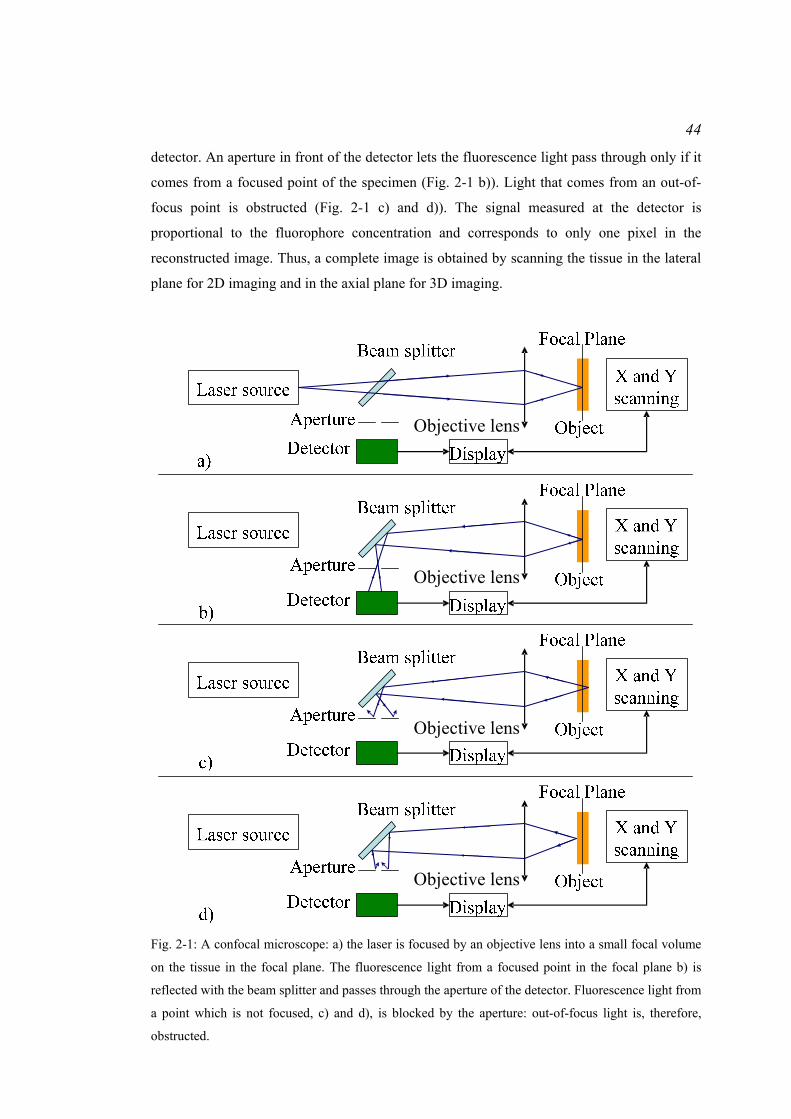
44
detector. An aperture in front of the detector lets the fluorescence light pass through only if it
comes from a focused point of the specimen (Fig. 2-1 b)). Light that comes from an out-of-
focus point is obstructed (Fig. 2-1 c) and d)). The signal measured at the detector is
proportional to the fluorophore concentration and corresponds to only one pixel in the
reconstructed image. Thus, a complete image is obtained by scanning the tissue in the lateral
plane for 2D imaging and in the axial plane for 3D imaging.
Objective lens
Objective lens
Objective lens
Objective lens
Fig. 2-1: A confocal microscope: a) the laser is focused by an objective lens into a small focal volume
on the tissue in the focal plane. The fluorescence light from a focused point in the focal plane b) is
reflected with the beam splitter and passes through the aperture of the detector. Fluorescence light from
a point which is not focused, c) and d), is blocked by the aperture: out-of-focus light is, therefore,
obstructed.
45
2.2.2 Fibered confocal microscopy
Optical fibres can replace the objective lens of a conventional confocal microscope for
remote laser delivery in order to perform optical biopsies. Mauna Kea Technologies, Paris,
developed such a system called Cellvizio®, a fibered confocal microscope that is usually
used in combination with a widefield endoscope. This system has been designed such that
individual cells can be distinguished; therefore, the resolution of the system must not exceed
a few microns (Vercauteren, 2008).
The fibered confocal microscope is made up of a Laser Scanning Unit (LSU) which
generates a laser beam at a wavelength of 488nm (Fig. 2-2 a)). The laser passes through each
individual fibre of a miniprobe which is made up of tens of thousands of optical fibres (Fig.
2-2 a) and b)). The laser beam from an optical fibre hits the biological tissue and fluorescent
light is emitted as well as a reflected laser beam. Only the mixture of lights coming from the
focal point passes through the optical fibre which has, therefore, the role of an aperture as
well. A dichroic filter filters wavelengths between 505nm and 700nm to keep only the
fluorescence light and send it to the detector. In order to build a whole image of the tissue
with typical dimensions of 500µm x 500µm, the laser beam is oriented to each individual
optical fibre with a set of two mirrors which rotate in two directions.
The raw image at the detector shows a strong honeycomb pattern, which makes it
hard to read by the user. A calibration step segments first the fibres to return a mapping
between the fibres and the sampling points of the raw image. Each sampling point
corresponds to a centre of a fibre. Secondly, the calibration step helps recover the background
signal Ib, and the signal for each fibre Is, and estimate the true signal Irestored for each fibre (Le
Goualher et al., 2004, and Perchant et al., 2005). The final image is reconstructed on a regular
grid by Gaussian weighting (Vercauteren et al., 2006).
a) b)
Fig. 2-2: The fibered confocal microscope by Mauna Kea Technologies, Paris: a) the system is made
up of a laser scanning unit and a miniprobe formed by tens of thousands of optical fibres; b) a laser
beam is sent to each individual optical fibre of the miniprobe for imaging one point of the fluorescent
tissue. A raw image of 500µm x 500µm is reconstructed at the detector.
Image not displayed for Copyright reasons

46
Fig. 2-3: a) Structure of the carotid artery: the thickness from the collagen layer to the endothelium
layer is approximately 70µm, b) whole tissue reconstruction after the scanning with the conventional
confocal microscope. The artery was scanned by moving the microscope objective lens. The mosaic
shows a series of connected patches. Each patch has been acquired for one position of the microscope
objective lens. The reconstructed mosaic is a maximum intensity projection of the slices acquired at
each depth of the tissue for each position of the objective lens. The bright green points correspond to
macrophages labelled with Invitrogen stain. A repetitive pattern is visible at the junction of the
patches: this is due to distortions from the objective lens (Courtesy Manfred Junemann Ramirez).
2.2.3 Experiment: Level of details reached by the fibered confocal microscope
Fibered Confocal Microscopy (FCM) returns images with typical dimensions of 500µm x
500µm. The purpose of this experiment was to determine the detail level that can be observed
in the images. To this aim, observations of a tissue by FCM and by conventional confocal
microscopy were compared. This experiment was done as part of a collaborative work with
Manfred Junemann Ramirez at University College London who prepared the experiment and
who ran the observation with the conventional confocal microscope.
2.2.3.1 Materials and method
For this experiment, a carotid artery of a rat was damaged in vivo using a balloon catheter.
The damage provoked an agglomeration of the macrophages around it. A fluorescent stain
(Invitrogen) was injected into the artery of the rat to bind to the macrophages. This stain
emits fluorescence for a 488nm excitation. Once the injection was done, the artery was taken
away for microscopic scanning with both a conventional confocal microscope and a fibered
confocal microscope.
The scanning with the conventional confocal microscope returned images of the
tissue at a depth of 45μm from the endothelial surface to the inner tissue (the tissue was
approximately 70μm thick). The artery structure is presented in Fig. 2-3 a). The carotid artery

47
images had a resolution of 1.46μm/pixel and can be presented by the maximum intensity
projection of a series of slices acquired at various depths into the tissue for each position of
the microscope objective lens, stitched together to create a whole mosaic image of the tissue
as shown in Fig. 2-3 b). This mosaic could be used as a map for the scanning during FCM.
The macrophages appear as points with the brightest intensities in the mosaic (Fig. 2-3 b)). A
650μm diameter miniprobe was used for the scanning with a fibered confocal microscope and
images with a pixel resolution of 0.83μm/pixel were obtained.
Once the corresponding images were acquired, they were visually matched to the
same region in the mosaic. The matching process was based on the recognition of the
macrophages arrangement in the microscopic image acquired during FCM and the
corresponding mosaic patch coming from conventional confocal microscopy.
2.2.3.2 Results and discussion
Fig. 2-4: Ex vivo interrogation of the cellular processes involved in the healing in a rat carotid artery
wound healing model by conventional confocal fluorescence microscopy (left) and by FCM (right)
(Courtesy for images acquired by conventional confocal microscopy Manfred Junemann Ramirez).
The inside walls of the carotid artery were damaged in vivo. A fluorochrome was administered after
injury to provide macrophage specific fluorescence staining. The macrophages moved to the damaged
regions. The artery was excised and scanned under a conventional confocal microscope and a year later
by FCM. Both imaging techniques showed similar groups of macrophages (bright green or white dots
in the images). The image acquired by conventional confocal microscopy was a z-projection of a xyz
tile scan stack. The image resolution was 1.46µm/pixel and the dimensions of one acquired image were
512 pixels x 512 pixels. The resolution of the FCM image was 0.83µm/pixel and its dimensions were
336 pixels x 480 pixels.

48
The carotid artery was scanned by FCM one year after the scanning with the conventional
confocal microscope. The artery was unfolded, hydrated and scanned from one extremity to
the other. The dimensions of the FCM images were 336pixels x 480pixels with a pixel
resolution of 0.83μm/pixel. Some microscopic images showed bright points, whose
dimensions were about 10μm and whose arrangement was similar to that of the bright points
(macrophages) in the mosaic (Fig. 2-4). The shape of the bright points helped also recognise
the corresponding mosaic patch.
This study showed that the scanning with a fibered confocal microscope allows
observations of cells with a diameter of approximately 10μm. Many macrophages could not,
however, be seen in the images acquired by FCM. The macrophages had been scanned a first
time with a conventional confocal microscope. The interaction of the laser beam with the
fluorescent region had already induced a loss of fluorescence. Moreover, the scanning of the
tissue with the fibered confocal microscope was performed a year later. Thus, macrophages
could have lost their fluorescence in the mean time. Finally, they were scanned several times
with the miniprobe, which induced the same interaction effect as that with the conventional
confocal microscope. A case was observed during the scanning with the fibered confocal
microscope and showed that a few macrophages lost their fluorescence while the miniprobe
was sweeping the corresponding region (Fig. 2-5). Thus, the lack of fluorescence seemed to
be the likeliest reason for not observing macrophages.
In conclusion, an observation of fluorescent structures by FCM returns similar results
as an observation by conventional confocal microscopy. Cells with a diameter of the order of
10μm are identifiable by FCM. Thus, the accuracy of the re-localisation technique has to be
of the order of 10μm. The next part presents a potential application of FCM and of the re-
localisation of a biopsy site.
a) b)
c) d)
165μm 165μm
165μm165μm
Fig. 2-5: Fluorescence loss of macrophages during the scanning with the fibered confocal microscope
(macrophages are surrounded by a red ring from a) to b)).

49
2.3 Potential combination with Magnetic Resonance Imaging for the
monitoring of the delivery of magnetic cells towards a site of interest
2.3.1 Delivery of cells using a magnetic resonance imaging system
A collaborative work with Riegler et al. (2010) demonstrated that cell delivery to specific
sites for tissue treatment could be done using Magnetic Resonance Targeting (MRT). This
delivery could be monitored using FCM. Johannes Riegler performed the MRT part of the
study. My contribution was to help set up the experiment with the fibered confocal
microscope and run the image acquisition. This section summarises the experiment.
2.3.1.1 Materials and method
Johannes Riegler’s idea consisted of using the force generated from the MR imaging coils to
form aggregates of magnetically labelled cells and to steer them. His aim was to demonstrate
with an experiment combining Magnetic Resonance Imaging (MRI) and FCM that when
injected through a tube placed in the permanent magnetic field of the MR scanner:
− The cells tend to form aggregates due to the dipole-dipole interactions.
− The cells tend to move along one direction which changes when a gradient is applied.
This experiment and the results were published in Riegler et al. (2011).
This principle was demonstrated using a phantom made up of pipes whose internal
diameter was 0.8mm designed by Johannes Riegler (Fig. 2-6 a)). Cells had a diameter of
10μm and were magnetically labelled. Given that their diameter is similar to that of the
macrophages studied in the previous section ‘2.2.3 Experiment: Level of details reached by
the fibered confocal microscope’, these cells could be observed by FCM after staining with a
fluorophore. The miniprobe of the fibered confocal microscope was, therefore, placed in the
phantom pipe and held tightly in order to acquire microscopic images at this position only
(Fig. 2-6 a)). The miniprobe was an MR-compatible probe of 7m long and 650μm diameter.
A 7m miniprobe was used in order to leave the fibered confocal microscope outside the MR
scanner room. The whole setup was introduced into the isocentre of a 9.4T MR scanner
(VNMRS, Varian, Inc. Palo Alto, CA) equipped with a bore of 60mm diameter (Fig. 2-6 b)).
Microscopic images were acquired with the fibered confocal microscope. Cells were in a
serum solution and were flushed into the phantom pipe using an infusion pump in order to
give them an initial speed. Control microscopic images were acquired when the setup was
outside the MR scanner. When the setup was inside the scanner, the cells were flushed at
different speeds to assess the impact of the flow velocity on the size of the aggregates.
Finally, the gradient was applied for short periods in order to change the direction of the cells.
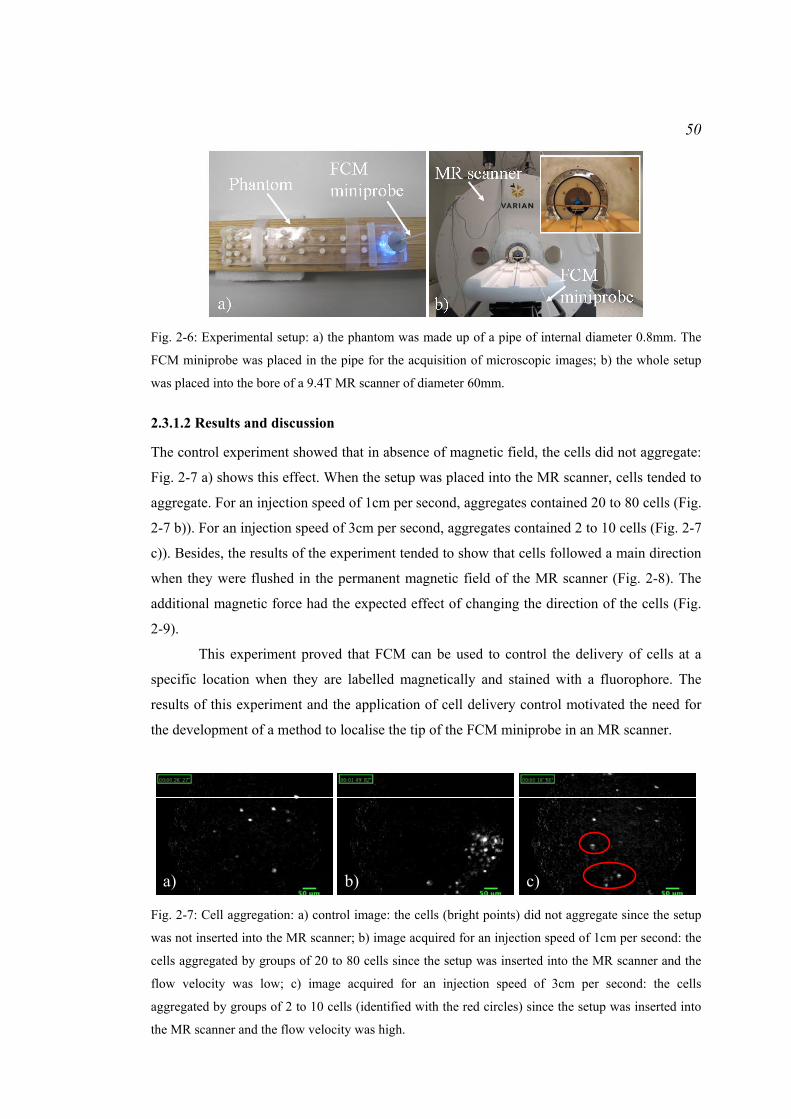
50
Fig. 2-6: Experimental setup: a) the phantom was made up of a pipe of internal diameter 0.8mm. The
FCM miniprobe was placed in the pipe for the acquisition of microscopic images; b) the whole setup
was placed into the bore of a 9.4T MR scanner of diameter 60mm.
2.3.1.2 Results and discussion
The control experiment showed that in absence of magnetic field, the cells did not aggregate:
Fig. 2-7 a) shows this effect. When the setup was placed into the MR scanner, cells tended to
aggregate. For an injection speed of 1cm per second, aggregates contained 20 to 80 cells (Fig.
2-7 b)). For an injection speed of 3cm per second, aggregates contained 2 to 10 cells (Fig. 2-7
c)). Besides, the results of the experiment tended to show that cells followed a main direction
when they were flushed in the permanent magnetic field of the MR scanner (Fig. 2-8). The
additional magnetic force had the expected effect of changing the direction of the cells (Fig.
2-9).
This experiment proved that FCM can be used to control the delivery of cells at a
specific location when they are labelled magnetically and stained with a fluorophore. The
results of this experiment and the application of cell delivery control motivated the need for
the development of a method to localise the tip of the FCM miniprobe in an MR scanner.
a) b) c)
Fig. 2-7: Cell aggregation: a) control image: the cells (bright points) did not aggregate since the setup
was not inserted into the MR scanner; b) image acquired for an injection speed of 1cm per second: the
cells aggregated by groups of 20 to 80 cells since the setup was inserted into the MR scanner and the
flow velocity was low; c) image acquired for an injection speed of 3cm per second: the cells
aggregated by groups of 2 to 10 cells (identified with the red circles) since the setup was inserted into
the MR scanner and the flow velocity was high.

51
1 2
3 4
Fig. 2-8: Results for the microscopic images acquired when the setup was placed into the MR scanner
without application of a gradient: the magnetic cells (bright points of approximately 10μm diameter)
were moving along one direction. Images 1, 2, 3, and 4 show the same cell (identified with the red
circle) in 4 consecutive microscopic images acquired with the fibered confocal microscope.
1 2
3 4
Fig. 2-9: Results for the microscopic images acquired when the setup was placed into the MR scanner
with application of a gradient: the cells moved along a different direction from that obtained when no
gradient was applied. Images 1, 2, 3, and 4 show the same cell (identified with the red circle) in 4
consecutive microscopic images acquired with the fibered confocal microscope.
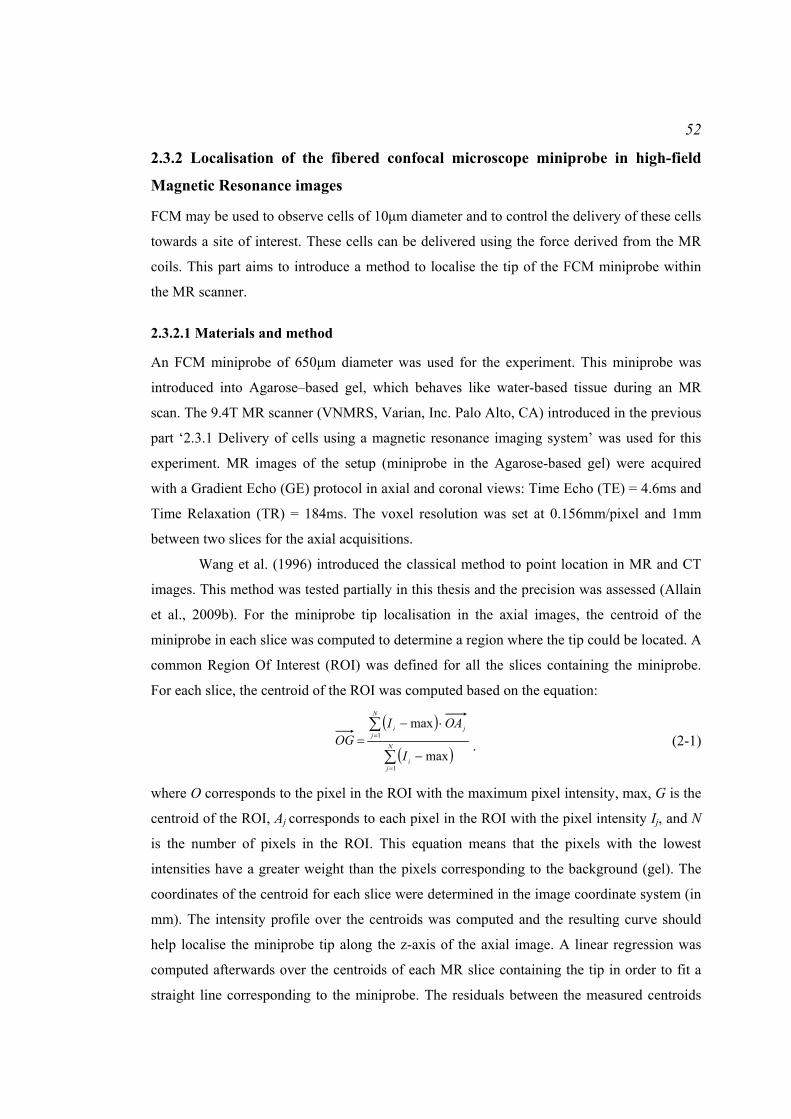
52
2.3.2 Localisation of the fibered confocal microscope miniprobe in high-field
Magnetic Resonance images
FCM may be used to observe cells of 10μm diameter and to control the delivery of these cells
towards a site of interest. These cells can be delivered using the force derived from the MR
coils. This part aims to introduce a method to localise the tip of the FCM miniprobe within
the MR scanner.
2.3.2.1 Materials and method
An FCM miniprobe of 650μm diameter was used for the experiment. This miniprobe was
introduced into Agarose–based gel, which behaves like water-based tissue during an MR
scan. The 9.4T MR scanner (VNMRS, Varian, Inc. Palo Alto, CA) introduced in the previous
part ‘2.3.1 Delivery of cells using a magnetic resonance imaging system’ was used for this
experiment. MR images of the setup (miniprobe in the Agarose-based gel) were acquired
with a Gradient Echo (GE) protocol in axial and coronal views: Time Echo (TE) = 4.6ms and
Time Relaxation (TR) = 184ms. The voxel resolution was set at 0.156mm/pixel and 1mm
between two slices for the axial acquisitions.
Wang et al. (1996) introduced the classical method to point location in MR and CT
images. This method was tested partially in this thesis and the precision was assessed (Allain
et al., 2009b). For the miniprobe tip localisation in the axial images, the centroid of the
miniprobe in each slice was computed to determine a region where the tip could be located. A
common Region Of Interest (ROI) was defined for all the slices containing the miniprobe.
For each slice, the centroid of the ROI was computed based on the equation:
( )
( )∑
∑
=
=
−
⋅−= N
ji
N
jji
I
OAIOG
1
1
max
max
.
(2-1)
where O corresponds to the pixel in the ROI with the maximum pixel intensity, max, G is the
centroid of the ROI, Aj corresponds to each pixel in the ROI with the pixel intensity Ij, and N
is the number of pixels in the ROI. This equation means that the pixels with the lowest
intensities have a greater weight than the pixels corresponding to the background (gel). The
coordinates of the centroid for each slice were determined in the image coordinate system (in
mm). The intensity profile over the centroids was computed and the resulting curve should
help localise the miniprobe tip along the z-axis of the axial image. A linear regression was
computed afterwards over the centroids of each MR slice containing the tip in order to fit a
straight line corresponding to the miniprobe. The residuals between the measured centroids
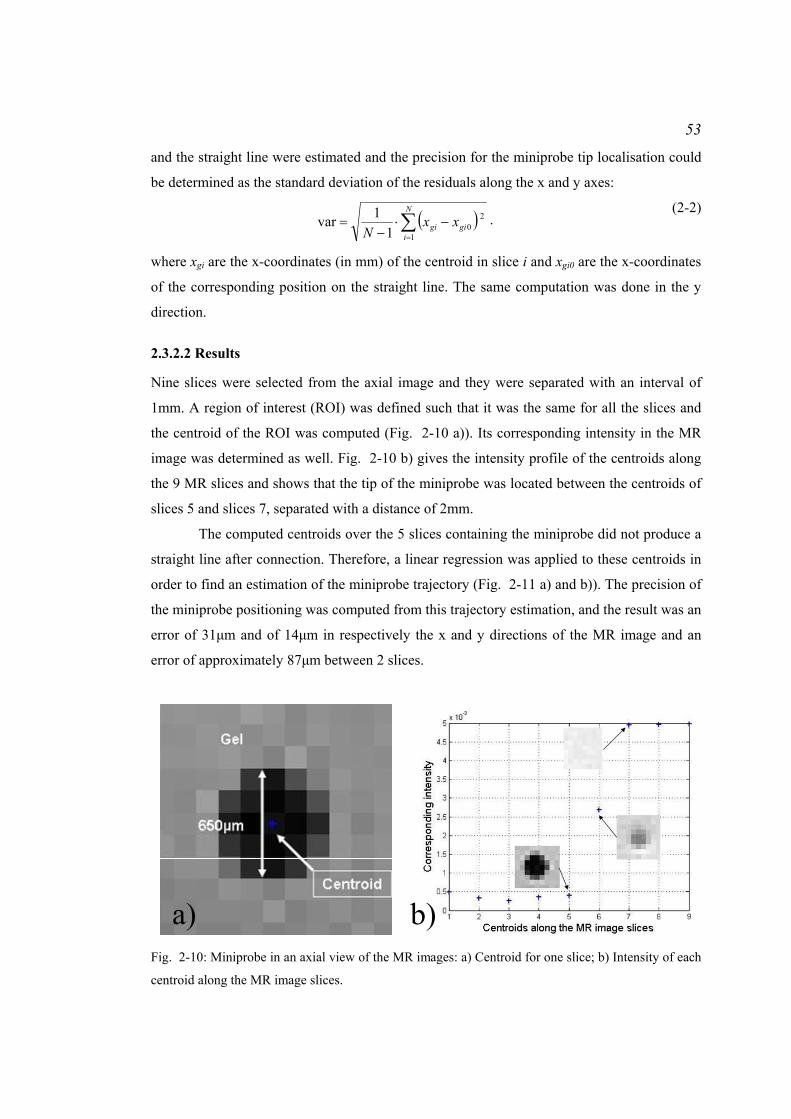
53
and the straight line were estimated and the precision for the miniprobe tip localisation could
be determined as the standard deviation of the residuals along the x and y axes:
( )∑=
−⋅−
=N
igigi xx
N 1
201
1var . (2-2)
where xgi are the x-coordinates (in mm) of the centroid in slice i and xgi0 are the x-coordinates
of the corresponding position on the straight line. The same computation was done in the y
direction.
2.3.2.2 Results
Nine slices were selected from the axial image and they were separated with an interval of
1mm. A region of interest (ROI) was defined such that it was the same for all the slices and
the centroid of the ROI was computed (Fig. 2-10 a)). Its corresponding intensity in the MR
image was determined as well. Fig. 2-10 b) gives the intensity profile of the centroids along
the 9 MR slices and shows that the tip of the miniprobe was located between the centroids of
slices 5 and slices 7, separated with a distance of 2mm.
The computed centroids over the 5 slices containing the miniprobe did not produce a
straight line after connection. Therefore, a linear regression was applied to these centroids in
order to find an estimation of the miniprobe trajectory (Fig. 2-11 a) and b)). The precision of
the miniprobe positioning was computed from this trajectory estimation, and the result was an
error of 31μm and of 14μm in respectively the x and y directions of the MR image and an
error of approximately 87μm between 2 slices.
a) b)
Fig. 2-10: Miniprobe in an axial view of the MR images: a) Centroid for one slice; b) Intensity of each
centroid along the MR image slices.
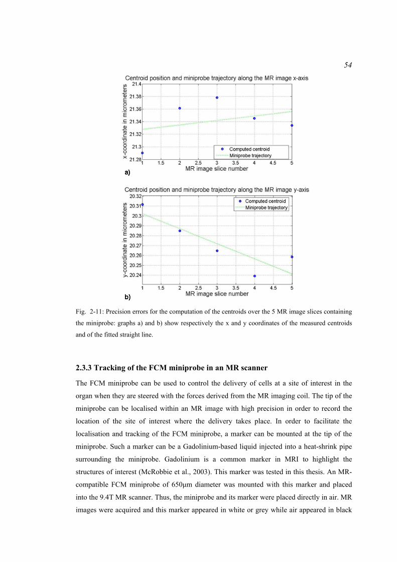
54
Fig. 2-11: Precision errors for the computation of the centroids over the 5 MR image slices containing
the miniprobe: graphs a) and b) show respectively the x and y coordinates of the measured centroids
and of the fitted straight line.
2.3.3 Tracking of the FCM miniprobe in an MR scanner
The FCM miniprobe can be used to control the delivery of cells at a site of interest in the
organ when they are steered with the forces derived from the MR imaging coil. The tip of the
miniprobe can be localised within an MR image with high precision in order to record the
location of the site of interest where the delivery takes place. In order to facilitate the
localisation and tracking of the FCM miniprobe, a marker can be mounted at the tip of the
miniprobe. Such a marker can be a Gadolinium-based liquid injected into a heat-shrink pipe
surrounding the miniprobe. Gadolinium is a common marker in MRI to highlight the
structures of interest (McRobbie et al., 2003). This marker was tested in this thesis. An MR-
compatible FCM miniprobe of 650μm diameter was mounted with this marker and placed
into the 9.4T MR scanner. Thus, the miniprobe and its marker were placed directly in air. MR
images were acquired and this marker appeared in white or grey while air appeared in black

55
(Fig. 2-12 a) and b)). In case the miniprobe needs to be used in air and imaged with an MR
scanner, Gadolinium-based gel can help highlight the miniprobe and the method to localise
the tip in an MR image could be used.
2.4 Conclusion
This chapter introduced initial experiments that demonstrated the potential of FCM to return
images showing structures of 10μm diameter. FCM can, therefore, be used to monitor the
delivery of cells for tissue treatment, for example. This chapter showed that cell delivery is
possible using an MR scanner. Thus, there is a potential need for recording the location of the
FCM miniprobe where the delivery was done in the MR image. A localisation method was
tested in this chapter and showed that the miniprobe tip could be localised with a precision of
the order of 10μm in MR images acquired with a 9.4T MR scanner. Although these
experiments demonstrated a potential interest for a combination of FCM and MRI, the
remainder of this thesis focuses on the development of a re-localisation method adapted to a
clinical application, the re-localisation of biopsy sites detected by optical biopsy during the
surveillance examination of Barrett’s Oesophagus.
a)air
Gadolinium-based marker
FCM miniprobe
b)
air
Gadolinium-based marker
FCM miniprobe
1mm 650μm
Fig. 2-12: Visualisation of an FCM miniprobe in an MR image acquired with a 9.4T MR scanner
(Varian): a) coronal view of the miniprobe mounted with a Gadolinium-based marker and placed in
air; b) axial view of the miniprobe mounted with a Gadolinium-based marker and placed in air.
56
Chapter 3 Literature Review: Possible Approaches for
Biopsy Site Re-localisation and Application for the
Surveillance Examination of Barrett’s Oesophagus
3.1 Introduction
Lesions detected in vivo and in situ by optical biopsy techniques need to be re-localised on
the macroscopic surface of the organ in order to go back to their position at a later time with
surgical instruments for tissue excision or for treatment, for example. As the lesions are
characterised by microscopic features that may have a size of the order of 10µm, the position
of the miniprobe has to be recorded ideally with an accuracy of the order of 10µm. The 2mm
diameter miniprobe is the physical instrument whose position can be tracked in the
macroscopic surface of the organ and indicates the presence of the lesions. Thus, the re-
localisation problem consists of tracking and recording the position of the miniprobe at the
macroscopic surface of the organ.
The choice of a re-localisation strategy may be mainly influenced by the clinical
application. As the main application of optical biopsy techniques is the early detection of
cancers in the oesophagus, colon, or lungs, the various methods and systems developed for
the tracking and guidance of surgical instruments in the macroscopic surface of the organ are
reviewed in this chapter. Their contribution to the re-localisation problem is also discussed.
The interventional examinations for the detection of cancers in the oesophagus, colon, and
lungs typically make use of an endoscope. The optical biopsy miniprobe is passed via the
working channel of this endoscope. Many systems developed for instrument tracking and
guidance made use of a 3D pre-operative image in order to extract the geometry of the organ.
During the interventions, the movement of the surgical instruments or of endoscopes was
tracked with positional sensors and registered in the pre-operative image. Other methods
made use of endoscopic images, only, to track the movement and record the positions of the
instruments. Finally, biopsy site re-localisation at the macroscopic surface of the organ may
also be useful for tissue treatment by cell delivery. Some results in Chapter 2 demonstrated
that Magnetic Resonance scanners have the potential to guide cell delivery. As these scanners
may also be used to acquire images of the oesophagus and colon, a potential strategy for
optical miniprobe tracking and guidance with Magnetic Resonance scanners are reviewed and
discussed.

57
The choice of a re-localisation strategy is a compromise between the clinical
application which may restrict the range of imaging systems and positional sensors, and the
accuracy of the methods developed for instrument tracking and guidance to a point of interest
at the macroscopic surface of the organ for tissue excision or treatment. As presented in
Chapter 1 ‘Introduction: The Need for Accurate Re-localisation of Microscopic Lesions in
their Macroscopic Context after Detection by Optical Biopsy’, the re-localisation of lesions is
particularly useful for biopsy sampling in the colon or in the oesophagus where the biopsy
sites may be invisible macroscopically. Thus, a re-localisation strategy is presented for such
applications. It is based on the epipolar geometry formed by the set of endoscopic images.
This chapter presents a method to recover the epipolar geometry.
3.2 Re-localising microscopic lesions in their macroscopic context
Various systems and methods have been developed for the tracking of the position of the tips
of surgical instruments, catheters, needles, probes, or forceps, and for their guidance at the
macroscopic surface of the organ during interventions.
3.2.1 Re-localising lesions within a pre-operative image
A variety of systems were developed for lesion localisation and instrument guidance during
interventions with the support of a pre-operative Computed Tomography (CT) or Magnetic
Resonance (MR) image (Deguchi et al., 2003, 2007; Helferty et al., 2002, 2007; Mori et al.,
2007, 2008). These were mainly developed for pulmonary applications, and make use of
endoscopes to provide interventional images. During the intervention with these systems,
lesions could be detected in the endoscopic images and their locations recorded in the 3D pre-
operative image thanks to a registration of the endoscope movement in the pre-operative
image (Fig. 3-1 a) and b)). The registration could be facilitated using positional sensors
mounted at the tip of the endoscope.
Fig. 3-1: Use of a virtual scene for the re-localisation of lesions detected during an endoscopic
examination: a) a real-time bronchoscopic image shows the biopsy needle in contact with the lesion; b)
the location of the lesion is computed in the virtual scene generated from a 3D pre-operative CT image.
As the bronchoscopic camera movement is tracked in the virtual scene, this scene can be used to guide
the bronchoscope and the surgical instruments to the lesion for tissue excision or treatment.
Image not displayed for Copyright reasons
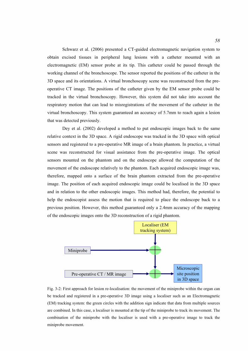
58
Schwarz et al. (2006) presented a CT-guided electromagnetic navigation system to
obtain excised tissues in peripheral lung lesions with a catheter mounted with an
electromagnetic (EM) sensor probe at its tip. This catheter could be passed through the
working channel of the bronchoscope. The sensor reported the positions of the catheter in the
3D space and its orientations. A virtual bronchoscopy scene was reconstructed from the pre-
operative CT image. The positions of the catheter given by the EM sensor probe could be
tracked in the virtual bronchoscopy. However, this system did not take into account the
respiratory motion that can lead to misregistrations of the movement of the catheter in the
virtual bronchoscopy. This system guaranteed an accuracy of 5.7mm to reach again a lesion
that was detected previously.
Dey et al. (2002) developed a method to put endoscopic images back to the same
relative context in the 3D space. A rigid endoscope was tracked in the 3D space with optical
sensors and registered to a pre-operative MR image of a brain phantom. In practice, a virtual
scene was reconstructed for visual assistance from the pre-operative image. The optical
sensors mounted on the phantom and on the endoscope allowed the computation of the
movement of the endoscope relatively to the phantom. Each acquired endoscopic image was,
therefore, mapped onto a surface of the brain phantom extracted from the pre-operative
image. The position of each acquired endoscopic image could be localised in the 3D space
and in relation to the other endoscopic images. This method had, therefore, the potential to
help the endoscopist assess the motion that is required to place the endoscope back to a
previous position. However, this method guaranteed only a 2.4mm accuracy of the mapping
of the endoscopic images onto the 3D reconstruction of a rigid phantom.
Miniprobe
Pre-operative CT / MR imageMicroscopic site position in 3D space
Localiser (EM tracking system)
Fig. 3-2: First approach for lesion re-localisation: the movement of the miniprobe within the organ can
be tracked and registered in a pre-operative 3D image using a localiser such as an Electromagnetic
(EM) tracking system: the green circles with the addition sign indicate that data from multiple sources
are combined. In this case, a localiser is mounted at the tip of the miniprobe to track its movement. The
combination of the miniprobe with the localiser is used with a pre-operative image to track the
miniprobe movement.

59
Szpala et al. (2005) presented a concept similar to Dey et al. (2002) applied to a
beating heart phantom. A rigid endoscope moved in space and acquired images of the heart.
The real phantom and the endoscope were tracked optically. A virtual scene was
reconstructed with the 3D model of the heart derived from the CT images. The virtual model
of the phantom was animated in synchronisation with the ECG signal of the ‘heartbeat’. The
presented method displayed the endoscopic images in front of the 3D model of the heart
moving dynamically in the virtual scene. This method took into account the organ motion.
The accuracy of the localisation of the endoscopic images at the surface of the organ was
1.4mm±1mm. Nevertheless, this method required optical sensors mounted on the heart
phantom and on the surgical instruments.
For the problem of re-localisation of lesions detected by optical biopsy, a 3D pre-
operative image can be used to provide the geometry of the organ of interest and a map of
lesions. A first strategy can be the use of the catheter mounted with the EM sensor to carry
the optical biopsy miniprobe (Fig. 3-2). When a lesion has been detected, the position of the
tip of the catheter reported by the EM sensor can be recorded in the space of the 3D pre-
operative image. The catheter is used after detection to guide instruments such as forceps to
the lesion using information from the EM sensor and visual feedback from the 3D pre-
operative image. However, the accuracy of the re-localisation of the lesions may be worse
than 2mm according to the results reported for these systems.
3.2.2 Re-localising lesions in endoscopic images
Using a 3D pre-operative image as a map for guidance of surgical instruments towards the
lesion may result in large inaccuracies for the instrument repositioning. Moreover, some
examinations for the detection of lesions may be based on interventional endoscopic images
only. For such examinations, the re-localisation problem consists, therefore, of guiding the
instruments to the lesion after detection with an optical miniprobe using real-time endoscopic
images only. As the lesion is located at the tip of the miniprobe, its tip has to be tracked in the
images. In addition to this, once the lesion has been detected, its location has to be updated in
the subsequent images acquired with a moving flexible endoscope.
Speidel et al. (2006) and Wengert et al. (2007) developed methods to segment
instruments, detect their tip, and compute their trajectories in space, in order to automate the
surgery and to control the movement of the instruments very accurately. However, these
proposed methods did not focus on the guidance of the instruments to a target point, while
Krupa et al. (2003) suggested a system that automatically positions the instruments in a
60
region of interest during laparoscopic examinations. The system was composed of a surgical
robot, an endoscopic optical camera, and an endoscopic laser pointing instrument holder. The
camera was inserted into a first incision point on the surface of the abdominal cavity and
placed in front of the region of interest. The instrument holder was moved by the robotic arm
and was inserted through a second incision point. It was mounted with a laser emitter to
project on the organ surface laser patterns that were visible in the camera image. The robot
moved the instrument inside the holder by an accurate depth based on the laser spot patterns.
Thus, the instrument was placed automatically in contact with the region of interest. Using a
laser pattern to indicate the location of the biopsy site is of interest for endoscopy since it is a
marker that does not destroy the tissue and that gives precise locations. However, this method
can work only if the camera and the laser probe remain still which is not the case for all
endoscopy examinations.
Voros et al. (2006) developed a method for instrument tracking in laparoscopic
images and guidance of the endoscope camera to a point of interest at the tissue surface. The
method used information on the 3D position of the insertion point in the abdominal cavity to
detect automatically and accurately the instruments in the laparoscopic images. The previous
positions of the tip of the instrument were localised in the current endoscopic image.
Unfortunately, these methods made the assumption that the camera of the rigid endoscope
remained still.
Methods and systems previously presented made use of additional hardware and rigid
endoscopes for the tracking and guidance of instruments in video images. However, space is
limited during endoscopic procedures and does not always allow an insertion of multiple
probes such as a laser holder. Also, optical biopsy techniques have been used mainly for
colonoscopic, gastroscopic, or pulmonary applications for which endoscopes are flexible and
keep moving within the organ. Thus, the guidance of instruments to the lesion must be
performed without additional hardware or any use of geometrical information that make the
assumption of rigidity of the endoscope.
Mori et al. (2002), Burschka et al. (2005), Hu et al. (2007), and Wang et al. (2008)
developed methods based only on image processing in order to track the motion of a flexible
endoscopic camera. The spatial transformations of the endoscopic camera that are rotations
and translations relative to the tissue surface were computed in order to determine the spatial
relation between endoscopic images. Such tracking may help reposition the endoscope near a
region of interest at the tissue surface. Hu et al. (2007) have applied the epipolar geometry
(Hartley and Zisserman, 2004) and the computer vision algorithms to endoscopic images
acquired during minimally invasive surgery of the heart. The goal of the work of Hu et al.

61
(2007) was to stitch the endoscopic images together to build a broader field of view and to
put these images together back to the same relative context. Two dimensional mosaics of
endoscopic images could be reconstructed. The mosaic was mapped onto a 3D model of the
organ of interest derived from a pre-operative image. This work may be used for the re-
localisation of lesions since the 2D mosaics can provide the endoscopist with a visual support
to know how he has to move the endoscope in order to observe a same region again. The 3D
pre-operative image can be used to derive a 3D reconstruction of the organ on which the
lesions detected in the endoscopic images can be mapped.
A strategy for lesion re-localisation may consist of determining the motion of the
endoscopic camera in relation to the imaged tissue in order to re-localise in the currently
acquired endoscopic image a lesion whose location is known in previously acquired
endoscopic images (Fig. 3-3). As shown in Hu et al. (2007), the recovery of this motion can
help compute the mapping from one endoscopic image where the lesion location is known to
another endoscopic image where it needs re-localising (Fig. 3-4). A registration of the camera
motion in a 3D pre-operative image has the potential to localise the endoscopic images and,
therefore, lesions in the 3D space of the organ.
Miniprobe
Endoscope
Pre-operative CT / MR image
Microscopic site position in
3D space
Microscopic site position in
endoscopic image
Fig. 3-3: Second approach for lesion re-localisation: the positions of the miniprobe tip are tracked in
the endoscopic images while the endoscope keeps moving. By tracking of the endoscope camera
movement in a pre-operative image, the positions of the miniprobe can be recorded in this image. Here
the miniprobe is used in combination with the endoscope in order to localise its position within the
endoscopic images. If the endoscope movement is tracked in the pre-operative image, the positions of
the miniprobe are known in the space of the image.
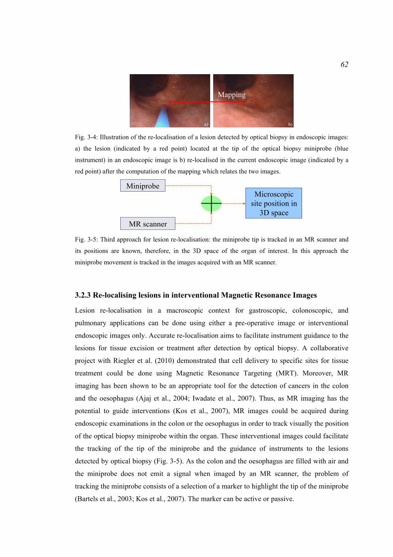
62
a) b)
Mapping
Fig. 3-4: Illustration of the re-localisation of a lesion detected by optical biopsy in endoscopic images:
a) the lesion (indicated by a red point) located at the tip of the optical biopsy miniprobe (blue
instrument) in an endoscopic image is b) re-localised in the current endoscopic image (indicated by a
red point) after the computation of the mapping which relates the two images.
MiniprobeMicroscopic
site position in 3D space
MR scanner Fig. 3-5: Third approach for lesion re-localisation: the miniprobe tip is tracked in an MR scanner and
its positions are known, therefore, in the 3D space of the organ of interest. In this approach the
miniprobe movement is tracked in the images acquired with an MR scanner.
3.2.3 Re-localising lesions in interventional Magnetic Resonance Images
Lesion re-localisation in a macroscopic context for gastroscopic, colonoscopic, and
pulmonary applications can be done using either a pre-operative image or interventional
endoscopic images only. Accurate re-localisation aims to facilitate instrument guidance to the
lesions for tissue excision or treatment after detection by optical biopsy. A collaborative
project with Riegler et al. (2010) demonstrated that cell delivery to specific sites for tissue
treatment could be done using Magnetic Resonance Targeting (MRT). Moreover, MR
imaging has been shown to be an appropriate tool for the detection of cancers in the colon
and the oesophagus (Ajaj et al., 2004; Iwadate et al., 2007). Thus, as MR imaging has the
potential to guide interventions (Kos et al., 2007), MR images could be acquired during
endoscopic examinations in the colon or the oesophagus in order to track visually the position
of the optical biopsy miniprobe within the organ. These interventional images could facilitate
the tracking of the tip of the miniprobe and the guidance of instruments to the lesions
detected by optical biopsy (Fig. 3-5). As the colon and the oesophagus are filled with air and
the miniprobe does not emit a signal when imaged by an MR scanner, the problem of
tracking the miniprobe consists of a selection of a marker to highlight the tip of the miniprobe
(Bartels et al., 2003; Kos et al., 2007). The marker can be active or passive.

63
Adding a micro-coil at the tip of the device is an active technique since the coil
resonates within the MR scanner at a different frequency from that of the surrounding tissues
(Fig. 3-6 a)). Therefore, the coil has high signal intensities in the MR image (bright regions)
while the tissues have lower signal intensities (darker regions). Among the active techniques,
there is also the use of electrified wire loops. A small direct current of about 10 to 150mA
induces distortions of the magnetic field within the MR scanner. Finally, self-resonant
radiofrequency circuits may be used as active techniques. Such circuits are coils or antennas
set on the device and tuned to the Larmor frequency of the MR scanner. In general, the active
techniques emit an accurate and robust signal, which is useful for the localisation of the
device in any situation. However, rapid radiofrequency heating occurs, making these
techniques not necessarily safe for in vivo applications (Bartels et al., 2003), and a strong
hardware development has to be done to make these techniques work correctly within an MR
environment.
Passive techniques allow avoiding the limitations of the active techniques and exploit
either the susceptibility effects of the markers (negative markers) or the signal enhancing
(positive markers). Negative markers are usually paramagnetic rings or ferrite-mixtures
(Mekle et al., 2006), which are set on the device, and which create susceptibility artefacts
when in contact with water molecules-based regions (Schenk, 1996; Nitatori, 1999). The
choice of the marker mainly depends on the application and on the analysed region. For
example, Dysprosium oxide markers may be used for catheter tracking in arteries
(Seppenwoolde et al., 2006), but an image acquisition protocol needs setting up to clearly
observe the artefacts. Although the use of negative markers is an easy method, the
visualisation of the markers mainly depends on their orientation about the magnetic field, on
the respiratory motion artefacts and on the presence of water molecules in contact with them.
Positive markers are also paramagnetic agents and they induce changes in the relaxation
times of water molecules in the surrounding regions. For example, a solution containing the
Gadolinium-DTPA complex shortens the T1 relaxation of the surrounding water molecules,
which results in a bright intensity for the Gadolinium-filled region and in a darker intensity
for the tissues (Fig. 3-6 b)). Gadolinium-Diethylenetriamine Pentaacetic Acid (DTPA)
complex in a water molecules-based solution is typically used as a contrast agent, but
coatings have to be designed in order to make surgical devices MR visible (Unal et al., 2006).
Although such coatings allow a good visualisation of the surgical tools and do not deteriorate
over time, they need to swell inside the body to make the device visible and they require a
careful chemical preparation.
64
a) b)
Fig. 3-6: Markers for instrument tracking in an MR image: a) a coil (indicated by the arrow) can be
mounted at the tip of the instrument, b) a Gadolinium-based coating can cover the instrument
(indicated by the arrows).
In conclusion, lesions may be localised at the tip of the optical biopsy miniprobe
within an MR image acquired during interventions. The re-localisation problem consists,
therefore, of selecting a marker to be mounted at the tip of the miniprobe to make it visible in
the image and of developing the method for computing the tip position within the MR image.
3.3 A clinical application: detection of cancers in Barrett’s
Oesophagus
The problem of lesion re-localisation in a macroscopic context may be solved with
interventional imaging systems or with a combination of positional sensors and pre-operative
images. Three main strategies were suggested, but they can be combined to give more
potential strategies. Nevertheless, the choice of a strategy may be mainly influenced by the
clinical application, by the imaging systems, and by other tools used for this application. As
the optical biopsy techniques were mainly used for the early detection of cancers in the
oesophagus, the lesion re-localisation method has been developed for the application of
endoscopic surveillance of Barrett’s Oesophagus (BO).
3.3.1 Cancers in Barrett’s Oesophagus and conventional diagnosis
Many of the published studies related to the clinical use of optical biopsies mentioned their
important role for the detection of lesions in the oesophagus in vivo and in situ. The optical
biopsy miniprobe can help target the biopsy sites in BO that need to be extracted for an
analysis by a histopathologist.
BO or Columnar Lined Oesophagus (CLO) is defined as a transformation of the
lower oesophageal mucosa from its usual stratified squamous non-keratinising phenotype to a
Image not displayed for Copyright reasons

65
metaplastic columnar epithelium (British British Society of Gastroenterology, 2005). This
may be visible macroscopically as a change of the oesophagus wall texture along a segment
typically developing as a region of altered mucosa above the normal gastro-oesophageal
junction (Fig. 3-7 a)). BO is a precursor lesion of oesophageal adenocarcinoma. During the
development of adenocarcinoma, the features of the epithelium change from ‘indefinite for
dysplasia’, to Low Grade Dysplasia (LGD), and to High Grade Dysplasia (HGD). A
dysplasia may manifest with macroscopic abnormalities such as a subtle granular appearance
to the mucosa of BO, isolated plaques of altered epithelium leading to a red-white mixed
lesion which is very unstable, or even a large mass region. However, in some cases, no
macroscopic manifestation occurs. LGD is the most frequently seen dysplasia. It may persist,
regress, or progress to HGD or adenocarcinoma. HGD carries a cancer risk of 16-59% within
5 years (Lovat et al., 2006). The risk is much lower for LGD. In the UK, the 5-year survival
rate in case of presence of adenocarcinoma is less than 10% (Lovat et al., 2006).
In order to make a positive diagnosis of BO, a segment of the suspected oesophageal
mucosa must be visible above the gastro-oesophageal junction and the clinical observational
suspicion must be confirmed histologically, mandating biopsies if a zone of change is
suspected. When pathology has been detected, the patient may enter a surveillance process.
Surveillance endoscopy examinations are undertaken at regular time intervals depending on
the diagnosed pathology. In surveillance endoscopy, quadrant biopsies are taken every 2cm in
the columnar segment together with biopsies of any visible lesion (Fig. 3-7 b)). If the
pathology is only chronic heartburn, the endoscopic surveillance is performed every 2 years.
For ‘Indefinite for dysplasia’, LGD, or HGD, the surveillance is performed more frequently
and the patient may even be sent to surgery. Both LGD and HGD may be managed by
ablation techniques removing all suspicious tissue, notably laser, photodynamic therapy
(PDT), and Argon Plasma Coagulation (APC) (British British Society of Gastroenterology,
2005).
Routine endoscopy is limited in its ability to identify dysplasia and sampling errors
are likely to occur if insufficient biopsies are taken (British Society of Gastroenterology,
2005). Unsuspected carcinoma in a BO segment may still be missed. Even if the quadrant
protocol is followed throughout the length of CLO and well into the normal squamous, errors
are still common. The main reason for missing these pathologies is maybe that epithelial
cancers and their precursors are frequently focal and can be distributed heterogeneously
across a wide field (Yun et al., 2006). Herein lies the next challenge which is establishing
where in the zone of change of the BO segment each biopsy should be taken from or has
come from.

66
Barrett’s Oesophagus segment
Normal Epithelium
Sites of excisions
Barrett’s Oesophagus segment
Boundary of Normal Epithelium
a) b) Fig. 3-7: Pathology and conventional diagnosis of BO: a) the BO segment is characterised by the
replacement of normal squamous epithelium by a metaplastic columnar epithelium; b) during a
surveillance examination, biopsies (black crosses) are taken at regular spaces along the BO segment.
3.3.2 Detection of the biopsy sites in BO by optical biopsy
Endoscopy is performed for diagnosis of BO and for guidance of forceps in order to take
biopsies in the BO segment. Optical biopsy techniques have the potential to improve
targeting of biopsy sites and to guide biopsy procedures during an endoscopic surveillance
examination of BO (Meining et al., 2007b.; Wallace et al., 2009).
An endoscope is introduced into the patient’s oesophagus (Fig. 3-8 a)). It returns real-
time videos of the tissue surface at a macroscopic level. This macroscopic view allows the
endoscopist to identify the zones of change at the tissue surface above the gastro-oesophageal
junction. Moreover, this view allows the endoscopist to guide the instruments passed via the
working channel of the endoscope such as optical biopsy miniprobes or biopsy forceps (Fig.
3-8 b) and c)).
The optical biopsy miniprobe is first passed via the single working channel of the
endoscope. The miniprobe is placed in contact with the tissue in order to scan it and two
views are available if microscopic imaging is performed: a macroscopic view from the
endoscope showing the miniprobe and a microscopic view from the miniprobe (Fig. 3-8 c)
and d)). If spectroscopy is performed, the miniprobe is still seen in the endoscopic view, but
it returns a spectrum instead of an image. Commonly, a tissue surface of approximately
0.5mm diameter is scanned. The optical biopsy has the benefit to allow the endoscopist to
make in real-time a diagnosis which is confirmed by histopathology a few weeks after the
examination. After tissue interrogation by optical biopsy, the miniprobe is taken out from the
endoscope working channel and replaced with forceps to take ‘colocalised’ biopsies at the
detected sites.
Image not displayed for Copyright reasons
67
Endoscope
Miniprobe
Oesophagus
Stomach
a) b)
c)
d) Fig. 3-8: The combination of macroscopic and microscopic views during endoscopy: a) An endoscope
is inserted into the patient’s oesophagus; b) the miniprobe is passed via the working channel of the
endoscope; c) the endoscope returns a macroscopic view of the analysed structure and the miniprobe
used for imaging the tissue at the cellular level is visible in the macroscopic view; d) a microscopic
image showing the cell structures is available at the same time.
For endoscopes with a single working channel, the biopsy excision consists of
guiding forceps to the biopsy site identified by optical biopsy. Typically during endoscopy
and especially during a surveillance examination of BO, the endoscope moves around the
detected biopsy site and air/water bubbles obstruct the endoscope camera field of view. Thus,
the task of taking ‘colocalised’ biopsies may be difficult.
3.3.3 Need for accurate re-localisation of biopsy sites during a surveillance
examination of BO
Optical biopsy techniques have the potential to improve detection and targeting of biopsy
sites during a surveillance examination of BO. The optical biopsy miniprobe is passed via the
working channel of the endoscope to take ‘colocalised’ biopsies. The excised tissue sample
has to match accurately the optical biopsy as the final diagnosis is done by the
histopathologist after the intervention.
The problem of an accurate matching between the excised tissue and the optical
measurement for many endoscopic applications combined with many optical biopsy
techniques has been raised in a series of published works like Wang et al. (2004), Dahr et al.
(2005), Evans et al. (2006), Lovat et al. (2006), and Pohl et al. (2008). Meining et al. (2007c.)
suggested that a potential sampling error may happen in case of focal lesions. Indeed, small
Image not displayed for Copyright reasons

68
focal lesions may be invisible macroscopically which makes the excision task more difficult
when the piece of tissue needs to be taken at the same location as the optical measurement.
Furthermore, the accurate matching is difficult to achieve since the endoscopist has to keep
the endoscope stable and still (Dahr et al., 2006).
A few methods were suggested for accurate matching. Lovat et al. (2006) explained
that a good match could be obtained thanks to the small indent that the miniprobe used for the
optical measurement left at the surface of the tissue. Nevertheless, 20% of the excised tissues
were not used for a comparison with the optical measurement since patient’s movement and
camera movement did not guarantee a perfect match. Pohl et al. (2008) created marks with
APC at the biopsy site locations during the quadrant process in BO for accurate re-
localisation of the lesions. The optical measurement was obtained next to each mark and
biopsies were taken from the same area and in the same endoscopic sequence. Nevertheless,
this technique burns the tissue. This may create a scar at the tissue surface which can lead to
erroneous diagnoses during future surveillance examinations of BO. Another method was
based on the tattooing of the tissue with ink. This was used for the re-localisation of small flat
polyps in colon in order to secure adequate margins during the surgery that occurs after the
colonoscopy (Botoman et al., 1994). The authors suggested tattooing the tissue with ink
before colon surgery. This ink is permanent which allows for preoperative radiation and other
delays without loss of the marked site. This also shortens operative times. However, these
methods do not prevent the endoscopist from taking useless biopsies. Indeed, a realistic
workflow would consist of interrogating first the tissue to target the biopsy site, of localising
this biopsy site secondly, and of extracting the tissue finally.
Physical makers at the tissue surface are not favourite methods to help for accurate
re-localisation of biopsy sites during a surveillance examination of BO. One of the three re-
localisation strategies presented earlier in this chapter or a combination of these strategies can
be useful for biopsy site re-localisation in the oesophagus. As the examination is based
principally on endoscopic images, an approach could be the development of an augmented
reality method for guidance of forceps to the biopsy site in the endoscopic images. The
workflow could be as follows: once the miniprobe has been removed from the endoscope
working channel, a virtual point or confidence region could be drawn in the digital
endoscopic images and tracked through them in order to indicate the location of the biopsy
site (Fig. 3-9). As mentioned earlier in this chapter, a mapping between endoscopic images is
required.
The re-localisation method has the potential to reduce the necessity of taking biopsies
and to target them better (Meining et al., 2007c.). An accurate re-localisation method is also

69
required for the validation of the accuracy of the diagnosis done by optical biopsy. For
example, so far, Meining et al. (2007c.) have done such a validation for tissues extracted from
BO, from the distal oesophagus, from the duodenum, or from rectal polyps. The validation
was done from lesions that were all clearly visible by endoscopy before the optical biopsy
was done. Therefore, the excised tissue matched accurately the optical measurement.
However, a more complete validation of the accuracy of the diagnosis done by optical biopsy
requires a comparison of the excised tissue with the optical measurement when the lesions are
invisible macroscopically. Finally, a re-localisation method may be useful not only for biopsy
sites during surveillance examination of BO, but also for flat polyp to determine the margins
for resection, or for microscopic colitis in vivo in colon (Meining et al., 2007a.). This method
could also be applied to any optical biopsy technique for which the miniprobe has to be in
contact with the tissue such as fibered confocal microscopy, elastic scattering spectroscopy,
or optical coherence tomography.
3.4 Computation of a mapping between endoscopic images
The previous discussions considered various methods to localise microscopic lesions within
their macroscopic context. An application may be the re-localisation of biopsy sites during a
surveillance examination of BO. As the examination is based only on video images, the re-
localisation problem consists of computing the mapping from one reference endoscopic
image where the biopsy site location is known to a target endoscopic image where the biopsy
site needs to be re-localised.
? ?
a) b)
c) d) Fig. 3-9: Illustration of the problem of re-localisation of the biopsy sites detected by optical biopsy
during an endoscopic surveillance of BO: a) endoscopic view of the gastro-oesophageal junction, b)
insertion of a 2mm diameter miniprobe, c) once the miniprobe has been removed, the biopsy site needs
to be re-localised (the ellipse and the interrogation mark illustrate the difficulty to decide where the re-
localised biopsy site is), d) the re-localisation is useful for the guidance of forceps since the endoscope
camera may have moved and the endoscopist may have lost the biopsy site from visual control.

70
a) b) Fig. 3-10: Endoscopic system: a) subsystems of the endoscope; b) description of the endoscope tip.
3.4.1 Endoscopic images acquired during a surveillance examination of BO
The surveillance examination of BO is based on the acquisition of real-time video images
with an endoscope inserted into the patient’s oesophagus.
An endoscope consists of several subsystems (Katzir, 1993). There are the endoscope
subsystems that provide illumination, irrigation, and suction (Fig. 3-10). Two light guides
provide illumination. An objective lens is placed in front of the imaging device and its
characteristics vary from endoscopes to endoscopes. Different lenses give different fields of
view and the focal distance may be different.
Clinical endoscopes used for this thesis were High Definition (HD) endoscopes
provided by Pentax Ltd. A miniature camera based on Charge-Coupled Device (CCD)
technology is attached to the distal end of the endoscope behind the objective lens. Colour
CCD cameras consist of a depositing of Red (R), Green (G), and Blue (B) long pass optical
filters on the individual light-sensitive elements of the camera. Each square of 4 pixels of the
colour CCD camera has one filtered red, one blue, and two green pixels since the human eye
is more sensitive to green (Cotton and Williams, 1996). The blue component of light whose
wavelength band is 400nm to 430nm and the green component whose wavelength band is
530nm to 550nm have a depth of penetration into the tissue that is superficial (Fig. 3-11).
Blue and Green illuminations correspond to the first and secondary peaks on the absorption
spectrum of haemoglobin. Red blood cells inside the vessels appear dark in the blue and
green channels of the acquired image. The Red component of light has longer bandwidth than
Blue and Green and its depth of penetration into the tissue is deeper. In order to illustrate this
property, an endoscopic image acquired during a surveillance examination of BO was split
into its RGB channels. The green and the blue channels showed clearly the vasculature (Fig.
3-12). The vessels had better contrast in the G component than in the B component since the
Image not displayed for Copyright reasons

71
B component has a superficial absorption into the tissue (Papagatsia et al., 2008). The biopsy
site re-localisation problem consists of determining the mapping between endoscopic images.
This mapping may be computed by recognition of similar structures in the images. As vessel
structures tend to be well contrasted in the G channel of endoscopic images, this channel was
used in this thesis to compute the mapping.
Fig. 3-11: Absorption of lights in the tissue: the blue and green lights highlight the vessels in the
superficial layers of the tissue. The red light and near-infrared (NIR) lights are less absorbed by the
tissue so penetrate deeper and can be reflected from deeper tissues.
Fig. 3-12: Red, Green, and Blue (RGB) channels of an endoscopic image: a) acquired endoscopic
image, b) R-channel of image a), c) G-channel of image a), and d) B-channel of image a).
Image not displayed for Copyright reasons
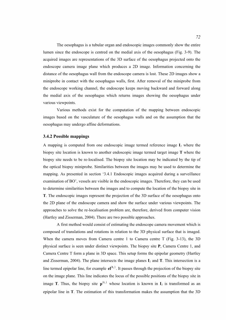
72
The oesophagus is a tubular organ and endoscopic images commonly show the entire
lumen since the endoscope is centred on the medial axis of the oesophagus (Fig. 3-9). The
acquired images are representations of the 3D surface of the oesophagus projected onto the
endoscope camera image plane which produces a 2D image. Information concerning the
distance of the oesophagus wall from the endoscope camera is lost. These 2D images show a
miniprobe in contact with the oesophagus walls, first. After removal of the miniprobe from
the endoscope working channel, the endoscope keeps moving backward and forward along
the medial axis of the oesophagus which returns images showing the oesophagus under
various viewpoints.
Various methods exist for the computation of the mapping between endoscopic
images based on the vasculature of the oesophagus walls and on the assumption that the
oesophagus may undergo affine deformations.
3.4.2 Possible mappings
A mapping is computed from one endoscopic image termed reference image I1 where the
biopsy site location is known to another endoscopic image termed target image T where the
biopsy site needs to be re-localised. The biopsy site location may be indicated by the tip of
the optical biopsy miniprobe. Similarities between the images may be used to determine the
mapping. As presented in section ‘3.4.1 Endoscopic images acquired during a surveillance
examination of BO’, vessels are visible in the endoscopic images. Therefore, they can be used
to determine similarities between the images and to compute the location of the biopsy site in
T. The endoscopic images represent the projection of the 3D surface of the oesophagus onto
the 2D plane of the endoscope camera and show the surface under various viewpoints. The
approaches to solve the re-localisation problem are, therefore, derived from computer vision
(Hartley and Zisserman, 2004). There are two possible approaches.
A first method would consist of estimating the endoscope camera movement which is
composed of translations and rotations in relation to the 3D physical surface that is imaged.
When the camera moves from Camera centre 1 to Camera centre T (Fig. 3-13), the 3D
physical surface is seen under distinct viewpoints. The biopsy site P, Camera Centre 1, and
Camera Centre T form a plane in 3D space. This setup forms the epipolar geometry (Hartley
and Zisserman, 2004). The plane intersects the image planes I1 and T. This intersection is a
line termed epipolar line, for example ( )1Iel . It passes through the projection of the biopsy site
on the image plane. This line indicates the locus of the possible positions of the biopsy site in
image T. Thus, the biopsy site ( )1Ip whose location is known in I1 is transformed as an
epipolar line in T. The estimation of this transformation makes the assumption that the 3D

73
physical surface that is imaged with an endoscope is stationary or may undergo affine
deformations (Hu et al., 2008a). As this transformation is a point to epipolar line mapping,
information from other reference endoscopic images have to be used to constrain the locus of
all of the possible locations of the biopsy site in T.
A second method is the Simultaneous Localisation And Mapping (SLAM) that has
been described and reported as employed during a gastroscopic examination for biopsy site
tracking in endoscopic images (Mountney et al., 2009). This method simultaneously builds
up a 3D map of the imaged physical surface knowing approximately the endoscope
movement in the 3D space and refines the endoscope camera position and orientation within
the map (Fig. 3-14). This method is based on an extension of the Kalman filter principle to
estimate the endoscope camera movement (Davison et al., 2007). When the endoscope
camera moves within the 3D physical surface, it is assumed that its velocity, its orientation,
and its position are known approximately. A positional sensor at the tip of the endoscope, for
example, can provide this information. This information assists the search for feature matches
from one endoscopic image acquired for the first camera position to a second endoscopic
image acquired for the current camera position. The map of features can be updated with new
features that were not visible in the previous image. The camera orientations and positions are
updated from the new map of features. Furthermore, the position of the biopsy site can be
tracked in the map.
Biopsy site P at the tissue surface
Camera centre 1
Camera centre T
I1
el
p e
T
(I1) (I1)
(I 1)
Fig. 3-13: Epipolar geometry formed by the pair of reference endoscopic image I1 and of target
endoscopic image T.
Update of the map
Localisation of theendoscope camera
within the map
Fig. 3-14: Illustration of the process of SLAM.
74
Two methods for the computation of the mapping between endoscopic images are
possible: recovery of the epipolar geometry and SLAM. SLAM has the advantage of building
a 3D map of the features of the imaged physical surface and of localising the endoscope
camera within this map. However, SLAM requires a smooth camera movement and a clear
FOV of the endoscopic camera. Air/water bubbles often obstruct the camera FOV or the
acquired images may be blurred because of a quick uncontrolled camera movement. In these
situations, features cannot be tracked anymore and the SLAM cannot update the camera
position and the feature map. As epipolar geometry is recovered between two images without
tracking movement of the endoscope camera, this approach is explored in this thesis. Finally,
the re-localisation method may be useful to re-localise a biopsy site in a future endoscopic
examination using reference images acquired during a previous examination. The SLAM can
be used only for the same examination. Epipolar geometry has the potential to solve the re-
localisation problem in this situation.
3.4.3 Computation of a mapping by recovery of the epipolar geometry
The approach for biopsy site re-localisation during a surveillance examination of BO makes
use of the epipolar geometry formed by endoscopic images.
The model of the endoscopic camera used in this thesis is the pinhole camera model
adapted to CCD cameras (Fig. 3-15) (Hartley and Zisserman, 2004). The camera is
characterised by a focal length f, scaling factors kx and ky in the x and y directions of the
image plane which correspond to the number of pixels per unit distance in the image
coordinate system, a skew parameter s which characterises the non-orthogonality of the
camera axes x and y and which is commonly assumed null, and a principal point which is the
projection of the camera centre C onto the image plane. When the image plane is attributed a
coordinate system (xI, yI) whose origin is located at the top left-hand corner of the image, the
principal point has coordinates (x0, y0) in this coordinate system. The biopsy site P at the 3D
physical surface whose coordinates in the camera coordinate system (xC, yC, zC) are (Px, Py,
Pz) projects onto the camera image plane as the point p(I) whose coordinates in the camera
coordinate system are (pxcam(I), pycam
(I), f) defined as:
( )
( )
z
yycam
z
xxcam
PP
fp
PP
fp
=
=
I
I
(3-1)
In the image coordinate system, the biopsy site coordinates are:

75
( )
( )00
00
yPP
yPP
fkp
xPP
xPP
fkp
z
yy
z
yyy
z
xx
z
xxx
+⋅=+=
+⋅=+=
⋅
⋅
α
α
I
I
(3-2)
Commonly homogeneous coordinates (u, v, w) in the image plane are used instead of the
image coordinates directly. These coordinates are related to the image coordinates such that:
( )
( )
wvp
wup
y
x
=
=
I
I
(3-3)
Thus, these coordinates are related to the coordinates in the endoscope camera coordinate
system with the camera calibration matrix or camera intrinsic parameter matrix K:
⎥⎥⎥
⎦
⎤
⎢⎢⎢
⎣
⎡
=
⎥⎥⎥⎥⎥
⎦
⎤
⎢⎢⎢⎢⎢
⎣
⎡
⋅⎥⎥⎥
⎦
⎤
⎢⎢⎢
⎣
⎡
=⎥⎥⎥
⎦
⎤
⎢⎢⎢
⎣
⎡
100
00
and
10100
0000
0
0
0
0
yx
P
PP
yx
wvu
y
x
z
y
x
y
x
αα
αα
K.
(3-4)
The matrix K expresses, therefore, the projection of the points on the 3D physical surface
onto the endoscope camera image plane.
During endoscopy, the camera moves with rotations ( )TIR ,1 and translations ( )TIt ,1
from the camera position Camera centre 1 to the camera position Camera centre T (Fig.
3-13). The resulting epipolar geometry can be described algebraically using the fundamental
matrix ( )TIF ,1 defined in Hartley and Zisserman (2004) as the composition of the camera
calibration matrix and the camera movement:
xC
yC
zCC
f
Biopsy site P(Px, Py, Pz)Biopsy site p(I)
(xp(I), yp
(I), f)
Endoscopicimage plane
Principal point (x0, y0, f)
xI
yI
( pxcam(I), pycam
(I), f )I
Fig. 3-15: Pinhole camera model and projection of the biopsy site onto the camera image plane.

76
input
output
Image I1Image T
Feature detection and matching
Fundamental matrix computation
( )TIF ,1 Fig. 3-16: Main steps for the recovery of the epipolar geometry.
( ) ( )[ ] ( ) ( ) ⋅⋅⋅⎥⎥⎥
⎦
⎤
⎢⎢⎢
⎣
⎡
−−
−⋅=⋅⋅⋅=
⎟⎟⎟
⎠
⎞
⎜⎜⎜
⎝
⎛= −− 1
,
12
13
23tr-1
,,tr-
987
654
321
, 111111
00
0
ITITITITITTI KRKKRtKFtt
tttt
fffffffff
(3-5)
1IK and KT are the camera calibration matrices at first and second positions. The camera
motion matrices ( )TIR ,1 and ( )TIt ,1
are expressed in a reference coordinate system that can be
the coordinate system of camera centre T, for example. The recovery of the epipolar
geometry consists of computing the fundamental matrix ( )TIF ,1.
In practice, ( )TIF ,1 is computed by detection of features in the images I1 and T (Fig.
3-16). These features are matched by studying their neighbourhood and by optimising a
similarity criterion between the neighbourhoods. The fundamental matrix is computed from
the set of matches.
3.5 Review of the methods for the recovery of the epipolar geometry
Epipolar geometry can be an approach to solve the biopsy site re-localisation. This part aims
to review the methods for the recovery of the epipolar geometry.
3.5.1 Endoscope camera calibration and correction of image distortions
Section ‘3.4.1 Endoscopic images acquired during a surveillance examination of BO’
introduced the system and components of an endoscope and the geometry of the endoscopic
images. The CCD camera that is mounted at the tip of the endoscope can be modelled as a
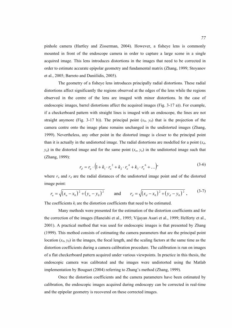
77
pinhole camera (Hartley and Zisserman, 2004). However, a fisheye lens is commonly
mounted in front of the endoscope camera in order to capture a large scene in a single
acquired image. This lens introduces distortions in the images that need to be corrected in
order to estimate accurate epipolar geometry and fundamental matrix (Zhang, 1999; Stoyanov
et al., 2005; Barreto and Daniilidis, 2005).
The geometry of a fisheye lens introduces principally radial distortions. These radial
distortions affect significantly the regions observed at the edges of the lens while the regions
observed in the centre of the lens are imaged with minor distortions. In the case of
endoscopic images, barrel distortions affect the acquired images (Fig. 3-17 a)). For example,
if a checkerboard pattern with straight lines is imaged with an endoscope, the lines are not
straight anymore (Fig. 3-17 b)). The principal point (x0, y0) that is the projection of the
camera centre onto the image plane remains unchanged in the undistorted images (Zhang,
1999). Nevertheless, any other point in the distorted image is closer to the principal point
than it is actually in the undistorted image. The radial distortions are modelled for a point (xd,
yd) in the distorted image and for the same point (xu, yu) in the undistorted image such that
(Zhang, 1999):
( )K+⋅+⋅+⋅+⋅= 63
42
211 uuuud rkrkrkrr . (3-6)
where ru and rd are the radial distances of the undistorted image point and of the distorted
image point:
( ) ( ) ( ) ( ) 20
20
20
20 and yyxxryyxxr ddduuu −+−=−+−= . (3-7)
The coefficients ki are the distortion coefficients that need to be estimated.
Many methods were presented for the estimation of the distortion coefficients and for
the correction of the images (Haneishi et al., 1995; Vijayan Asari et al., 1999; Helferty et al.,
2001). A practical method that was used for endoscopic images is that presented by Zhang
(1999). This method consists of estimating the camera parameters that are the principal point
location (x0, y0) in the images, the focal length, and the scaling factors at the same time as the
distortion coefficients during a camera calibration procedure. The calibration is run on images
of a flat checkerboard pattern acquired under various viewpoints. In practice in this thesis, the
endoscopic camera was calibrated and the images were undistorted using the Matlab
implementation by Bouguet (2004) referring to Zhang’s method (Zhang, 1999).
Once the distortion coefficients and the camera parameters have been estimated by
calibration, the endoscopic images acquired during endoscopy can be corrected in real-time
and the epipolar geometry is recovered on these corrected images.

78
b) c)a)Principal point (x0, y0)
Distorted image coordinates (xd, yd)
Undistorted image coordinates (xu, yu)
Fig. 3-17: Barrel distortions in endoscopic images: a) barrel distortions are such that a point appears
closer to the principal point than it is in reality and the distortions are greater on the sides of the image;
b) illustration of barrel distortions on a flat checkerboard pattern imaged with an endoscope mounted
with a fisheye lens at the tip; c) endoscopic image of the flat checkerboard after correction for
distortions.
3.5.2 Feature detection and matching
A first step of the recovery of the epipolar geometry consists of detecting features in each
image and of finding their matches in another image. Automatic methods for feature
detection and matching are necessary for a clinical application such as the re-localisation of
biopsy sites during a surveillance examination of Barrett’s Oesophagus (BO). Features can be
detected and matched with feature trackers or with techniques based on descriptors.
3.5.2.1 Feature trackers: the example of the Lucas-Kanade tracker
During an endoscopy examination in the oesophagus, the camera usually moves smoothly.
The acquired images of the video stream show the tissue surface under various viewpoints. It
is, therefore, possible to use feature trackers that detect features in a first reference image Ii
and track them through the images of the video stream up to the target image T. These
features sit at the centre of a pixel-based searching window and the tracking consists of
finding in the next images where this window is located. Two feature trackers have been
mainly used for endoscopic images: block matching for bronchoscopic images (Mori et al.,
2002) and the Lucas-Kanade (LK) tracker for minimally invasive surgery of the heart (Lucas
and Kanade, 1981; Mountney et al. 2006; Hu et al., 2007, 2009). Block matching considers
that the pixel window undergoes only translations from video images to video images whilst
the LK tracker takes into account affine deformations of the window (i.e. rotations and
shearing). As the re-localisation has to be performed between a reference image Ii and a
target image T showing the tissue region under a different viewpoint (Fig. 3-18), the changes
of the shape of the pixel window can be described by an affine transformation and the LK
tracker is more appropriate.
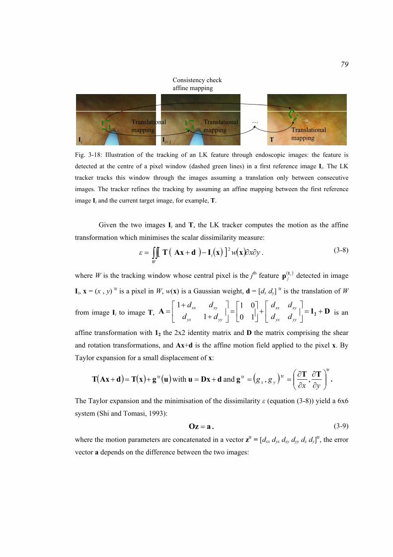
79
…
Ii Ii+1 T
Translational mapping
Translational mapping Translational
mapping
Consistency check affine mapping
Fig. 3-18: Illustration of the tracking of an LK feature through endoscopic images: the feature is
detected at the centre of a pixel window (dashed green lines) in a first reference image Ii. The LK
tracker tracks this window through the images assuming a translation only between consecutive
images. The tracker refines the tracking by assuming an affine mapping between the first reference
image Ii and the current target image, for example, T.
Given the two images Ii and T, the LK tracker computes the motion as the affine
transformation which minimises the scalar dissimilarity measure:
( ) ( )[ ] ( )∫∫ ∂∂−+=W
i yxwε xxIdAxT 2 . (3-8)
where W is the tracking window whose central pixel is the jth feature ( )ijIp detected in image
Ii, x = (x , y) tr is a pixel in W, w(x) is a Gaussian weight, d = [dx dy] tr is the translation of W
from image Ii to image T, D1A 2 +=⎥⎦
⎤⎢⎣
⎡+⎥
⎦
⎤⎢⎣
⎡=⎥
⎦
⎤⎢⎣
⎡+
+=
yyyx
xyxx
yyyx
xyxx
dddd
dddd
1001
11
is an
affine transformation with 12 the 2x2 identity matrix and D the matrix comprising the shear
and rotation transformations, and Ax+d is the affine motion field applied to the pixel x. By
Taylor expansion for a small displacement of x:
( ) ( ) ( ) ( )tr
trtrtr ,, and with ⎟⎟⎠
⎞⎜⎜⎝
⎛∂∂
∂∂
==+=+=+yx
gg yxTTgdDxuugxTdAxT .
The Taylor expansion and the minimisation of the dissimilarity ε (equation (3-8)) yield a 6x6
system (Shi and Tomasi, 1993):
aOz = . (3-9)
where the motion parameters are concatenated in a vector ztr = [dxx dyx dxy dyy dx dy]tr, the error
vector a depends on the difference between the two images:
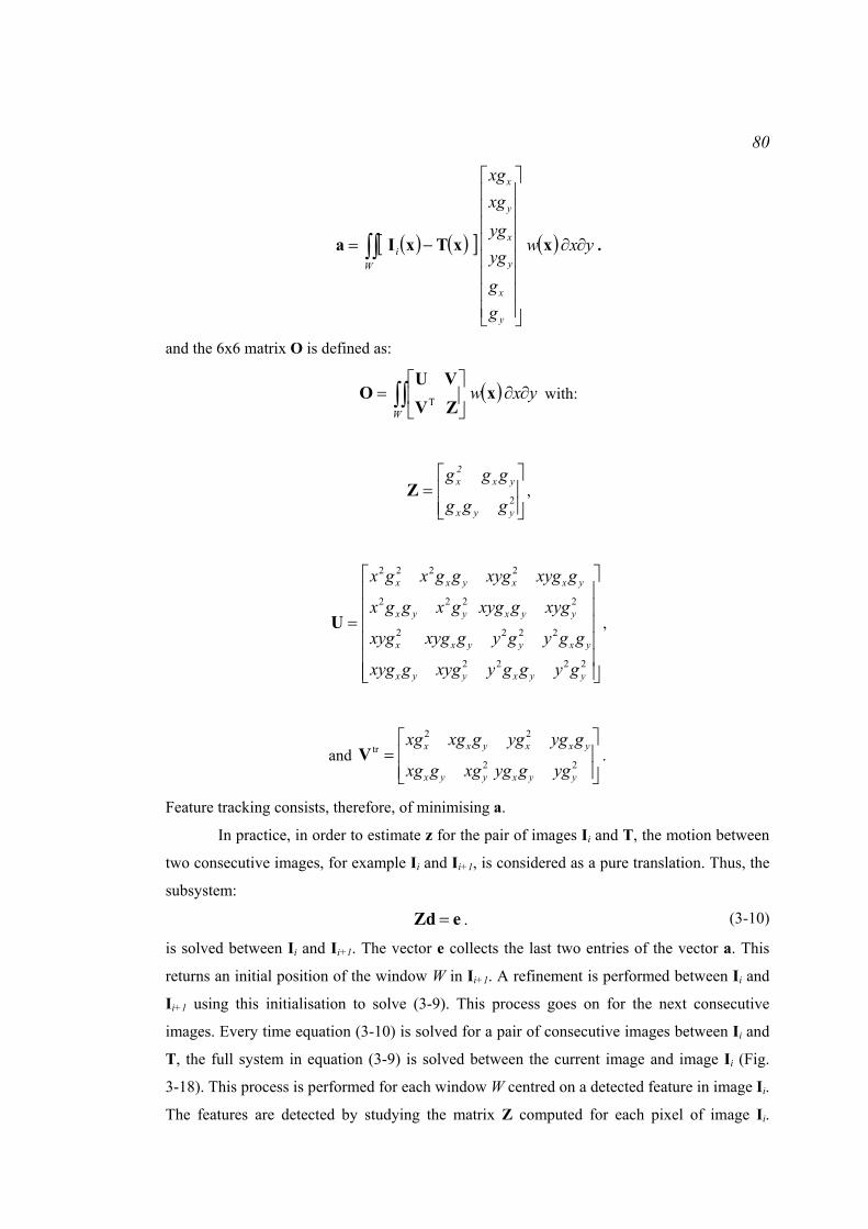
80
( ) ( )[ ] ( ) yxw
gg
ygygxgxg
W
y
x
y
x
y
x
i ∂∂
⎥⎥⎥⎥⎥⎥⎥⎥
⎦
⎤
⎢⎢⎢⎢⎢⎢⎢⎢
⎣
⎡
−= ∫∫ xxTxIa .
and the 6x6 matrix O is defined as:
( ) yxwW
∂∂⎥⎦
⎤⎢⎣
⎡= ∫∫ x
ZVVU
OT with:
⎥⎥⎦
⎤
⎢⎢⎣
⎡=
2yyx
yx2x
ggg
gggZ ,
⎥⎥⎥⎥⎥⎥
⎦
⎤
⎢⎢⎢⎢⎢⎢
⎣
⎡
=
2222
2222
2222
2222
yyxyyx
yxyyxx
yyxyyx
yxxyxx
gyggyxyggxyg
ggygygxygxyg
xyggxyggxggx
gxygxygggxgx
U ,
and ⎥⎥⎦
⎤
⎢⎢⎣
⎡=
22
22tr
yyxyyx
yxxyxx
yggygxggxg
gygyggxgxgV .
Feature tracking consists, therefore, of minimising a.
In practice, in order to estimate z for the pair of images Ii and T, the motion between
two consecutive images, for example Ii and Ii+1, is considered as a pure translation. Thus, the
subsystem:
eZd = . (3-10)
is solved between Ii and Ii+1. The vector e collects the last two entries of the vector a. This
returns an initial position of the window W in Ii+1. A refinement is performed between Ii and
Ii+1 using this initialisation to solve (3-9). This process goes on for the next consecutive
images. Every time equation (3-10) is solved for a pair of consecutive images between Ii and
T, the full system in equation (3-9) is solved between the current image and image Ii (Fig.
3-18). This process is performed for each window W centred on a detected feature in image Ii.
The features are detected by studying the matrix Z computed for each pixel of image Ii.

81
Indeed, the matrix Z gives information about the local texture around the pixel (Shi and
Tomasi, 1994). If the two eigenvalues of Z are small, the intensity in the window W is
roughly constant. A large and a small eigenvalue correspond to an edge. Two large
eigenvalues correspond to corners or salt and pepper textures that can be tracked reliably.
Therefore, the N features whose windows have the largest eigenvalues are selected.
3.5.2.2 Feature detection in the image scale-space and matching of descriptors: the
example of the Scale Invariant Feature Transform
During endoscopy examinations, the endoscope camera field of view may be obstructed with
air/water bubbles (Mori et al., 2005). The camera may also move too quickly sometimes
which returns a series of blurred images (Mori et al., 2005). Finally, specularities due to a
certain angle of the endoscope illumination channel relative to the wet tissue surface may
appear in the images (Mori et al., 2005). Therefore, features cannot be tracked with the LK
tracker, for example. An alternative to the trackers can be the feature detectors in the image
scale-space and the matching of the features based on their descriptors (Lindeberg, 1998;
Mikolajczyk and Schmid, 2005a; Mikolajczyk et al., 2005b). These detectors aim to identify
features in images of an object at locations and scales that can be repeatedly assigned under
differing views of the object (Lowe, 2004). Such stable features can be searched across all of
the possible scales of the image using a function of scale known as scale-space (Witkin,
1983). Koenderick (1984) and Lindeberg (1994) demonstrated that the Gaussian function can
be used as the scale-space kernel. Therefore, the scale-space L of an image Ii for the scale s is
defined as the convolution of Ii with the Gaussian kernel G such that:
( ) ( ) ( ) ( )yx,es
yx,sy,x,syx is
yx
i IIL ∗=∗=+
− 2
22
222
1G,,π
. (3-11)
Stable features can be found as extrema in the Laplacian of Gaussian or difference of
Gaussians of the image Ii, for example (Mikolajczyk et al., 2001).
Once a feature location has been detected, a local description or descriptor can be
computed for matching the features from two images. A descriptor can be a vector containing
information about the gradients in a local neighbourhood of the detected feature (Lindeberg,
1997; Mikolajczyk et al., 2002; Mikolajczyk et al., 2004; Lowe, 2004; Mikolajczyk et al.,
2005b). Classical techniques for feature detection and matching based on the feature detectors
are the Scale Invariant Feature Transform (SIFT) (Lowe, 2004) and the scale and affine
invariant interest point detectors (Lindeberg, 1997; Mikolajczyk et al., 2002; Mikolajczyk et
al., 2004; Mikolajczyk et al., 2005b). The SIFT and the scale invariant interest point detectors
have been used for detection and matching of features in endoscopic images especially for
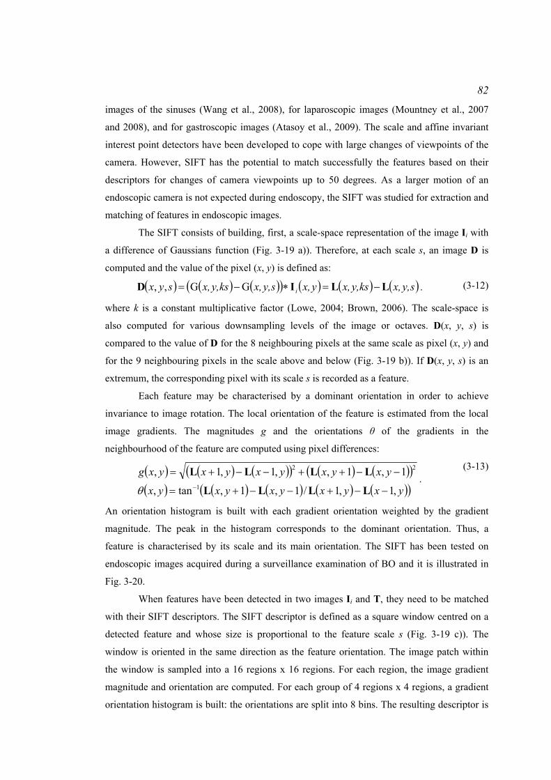
82
images of the sinuses (Wang et al., 2008), for laparoscopic images (Mountney et al., 2007
and 2008), and for gastroscopic images (Atasoy et al., 2009). The scale and affine invariant
interest point detectors have been developed to cope with large changes of viewpoints of the
camera. However, SIFT has the potential to match successfully the features based on their
descriptors for changes of camera viewpoints up to 50 degrees. As a larger motion of an
endoscopic camera is not expected during endoscopy, the SIFT was studied for extraction and
matching of features in endoscopic images.
The SIFT consists of building, first, a scale-space representation of the image Ii with
a difference of Gaussians function (Fig. 3-19 a)). Therefore, at each scale s, an image D is
computed and the value of the pixel (x, y) is defined as:
( ) ( ) ( )( ) ( ) ( ) ( )sy,x,ksy,x,yx,sy,x,ksy,x,syx i LLID −=∗−= GG,, . (3-12)
where k is a constant multiplicative factor (Lowe, 2004; Brown, 2006). The scale-space is
also computed for various downsampling levels of the image or octaves. D(x, y, s) is
compared to the value of D for the 8 neighbouring pixels at the same scale as pixel (x, y) and
for the 9 neighbouring pixels in the scale above and below (Fig. 3-19 b)). If D(x, y, s) is an
extremum, the corresponding pixel with its scale s is recorded as a feature.
Each feature may be characterised by a dominant orientation in order to achieve
invariance to image rotation. The local orientation of the feature is estimated from the local
image gradients. The magnitudes g and the orientations θ of the gradients in the
neighbourhood of the feature are computed using pixel differences:
( ) ( ) ( )( ) ( ) ( )( )( ) ( ) ( ) ( ) ( )( )yxyxyxyxyx
yxyxyxyxyxg
,1,1/1,1,tan,
1,1,,1,1,1
22
−−+−−+=
−−++−−+=− LLLL
LLLL
θ.
(3-13)
An orientation histogram is built with each gradient orientation weighted by the gradient
magnitude. The peak in the histogram corresponds to the dominant orientation. Thus, a
feature is characterised by its scale and its main orientation. The SIFT has been tested on
endoscopic images acquired during a surveillance examination of BO and it is illustrated in
Fig. 3-20.
When features have been detected in two images Ii and T, they need to be matched
with their SIFT descriptors. The SIFT descriptor is defined as a square window centred on a
detected feature and whose size is proportional to the feature scale s (Fig. 3-19 c)). The
window is oriented in the same direction as the feature orientation. The image patch within
the window is sampled into a 16 regions x 16 regions. For each region, the image gradient
magnitude and orientation are computed. For each group of 4 regions x 4 regions, a gradient
orientation histogram is built: the orientations are split into 8 bins. The resulting descriptor is

83
a vector of 4x4x8 entries where each entry is a function of the magnitudes. This vector is
normalised to unit length. Matching a feature in Ii to another feature in T consists of looking
for a descriptor in T which is at a minimal Euclidean distance from a descriptor in Ii. The
match is accepted if and only if the ratio of the Euclidean distances between the first and the
second best match is greater than a threshold, set manually.
a)
b)
Feature at given scale and orientation
1 region
16 regions
1 orientation histogram
c) Fig. 3-19: Detection of SIFT features and computation of their descriptors: a) the scale-space of the
image is built: for each octave or downsampling level of the image, the image is repeatedly convolved
with a Gaussian kernel. Adjacent Gaussian images are subtracted to generate the Difference of
Gaussian images; b) Extrema of the Difference of Gaussian images are detected by comparison of the
pixel (marked with X) to its 8 neighbours at the same scale and to its 18 neighbours in the lower and
higher scales; c) the descriptor is a window centred on the detected feature. The size of the window is
proportional to the scale of the feature and is oriented in the same direction as the feature orientation.
The window is divided in 16 regions x 16 regions and for each region, the gradient magnitude and
orientation are computed. Regions are stacked into 4 regions x 4 regions in order to build an
orientation histogram. The descriptor is a vector whose entries are the orientation histograms.
a) b)
c) d) Fig. 3-20: Example of a SIFT feature in two different views of the same physical surface of the
oesophagus acquired during an endoscopy: a) a feature is detected in a reference image Ii at the
intersection of vessels. Its location is at the centre of the circle whose radius is proportional to the scale
at which the feature was detected. The drawn radius indicates the feature orientation; b) zoomed image
on the feature detected in a); c) the matching feature corresponding to the same anatomical point is
detected in the target image T; d) zoomed image on the feature.
Image not displayed for Copyright reasons

84
3.5.3 Computation of the fundamental matrix
The fundamental matrix ( )TIF ,i can be computed using the features in images Ii and T that are
matched. Some of these matches are correct since they obey the epipolar geometry and are
termed inliers (Torr, 1995; Torr and Davidson, 2003). Others are incorrect matches which
refer to a pair of features that do not correspond to the same anatomical point, which are
inconsistent with the epipolar geometry, and which are termed outliers (Torr, 1995; Torr and
Davidson, 2003). The feature detection and matching techniques return a set of L matches D =
{ ( )ijIp , pj}j=1..L with ( ) ( ) ( )[ ] tr
1,, iiijyjxj pp IIIp = , a feature in Ii which matches pj = [pjx, pjy, 1] tr, a
feature in T. The fundamental matrix is estimated from this set of matches.
3.5.3.1 Properties of the fundamental matrix
The fundamental matrix ( )TIF ,i can be defined as the mapping between two endoscopic
images. A feature ( )ijIp in image Ii is mapped onto T as an epipolar line ( )i
jIel = ( )TIF ,i
. ( )ijIp =
( ) ( ) ( )[ ] tr,, iii
jmjyjx elelel III (Hartley and Zisserman, 2004). This line passes through the matching
feature pj. Thus, pjtr. ( )i
jIel = pj
tr. ( )TIF ,i. ( )i
jIp = 0.
In practice, features are detected with errors due to the noise in the camera which are
classically assumed independently and identically distributed Gaussian errors with standard
deviation σ (Luong and Faugeras, 1996). Therefore, the feature pj does not lie exactly on the
epipolar line ( )ijIel = ( )TIF ,i
. ( )ijIp and pj
tr. ( )TIF ,i. ( )i
jIp is equal to a residual error ( )i
je I termed
algebraic residual (Hartley and Zisserman, 2004):
( )( )
( )( ) 2,
tr2i
i
ijjje I
TII pFp ⋅⋅= . (3-14)
The fundamental matrix ( )TIF ,i can be determined by least squares as the vector that
minimises the squared algebraic residuals ( )ije I over the entire set of matches D = { ( )i
jIp ,
pj}j=1..L.
The fundamental matrix encapsulates the translation ( )TIt ,i and rotation ( )TIR ,i
of the
camera as shown in equation (3-5). A cross-product between ( )TIt ,i and ( )TIR ,i
is applied
which is equivalent to a multiplication such that:
( )[ ] ( ) ( )TITITI RRt ,
12
13
23
,,
00
0
iii
tttt
tt⋅
⎥⎥⎥
⎦
⎤
⎢⎢⎢
⎣
⎡
−−
−=⋅ .
(3-15)
85
The determinant of [ ( )TIt ,i] is null. Thus, the determinant of ( )TIF ,i
is also zero. That is to say,
the rank of ( )TIF ,i should be 2. Finally, ( )TIF ,i
is determined up to a scale factor. The additional
constraint || ( )TIF ,i|| = 1 can be applied (Torr and Fitzgibbon, 2004).
Many methods were presented for the computation of the fundamental matrix by
taking into account its properties (Longuet-Higgins, 1981; Hartley, 1995; Luong and
Faugeras, 1996; Csurka, 1997; Zhang, 1998).
3.5.3.2 Computation of the fundamental matrix from a minimal set of matches
Longuet-Higgins (1981) introduced the first landmark method for the computation of the
fundamental matrix, the eight-point algorithm. It was improved later by Hartley (1995) to
make it more robust to the noise on the features, which serve as inputs for the computation of
the fundamental matrix. The fundamental matrix can also be estimated from the seven-point
algorithm (Deriche et al., 1994).
The eight-point algorithm builds up a set of 8 equations of the form
( )( ) 0,
tr =⋅⋅ i
i jjI
TI pFp between the matches ( )ijIp of image Ii and pj of image T. This leads to a
system of the form: A ( )TIf ,i = 0 where A and ( )TIf ,i
are defined as follows:
( ) 0
1
1
1
9
8
7
6
5
4
3
2
1
)(8
)(888
)(88
)(888
)(88
)(8
)()()()()()(
)(1
)(111
)(11
)(111
)(11
)(1
, =
⎟⎟⎟⎟⎟⎟⎟⎟⎟⎟⎟⎟⎟
⎠
⎞
⎜⎜⎜⎜⎜⎜⎜⎜⎜⎜⎜⎜⎜
⎝
⎛
⎟⎟⎟⎟⎟⎟⎟
⎠
⎞
⎜⎜⎜⎜⎜⎜⎜
⎝
⎛
=
fffffffff
pppppppppppp
pppppppppppp
pppppppppppp
iiiiii
iiiiii
iiiiii
i
yxyyyyxxxyxx
jyjxjyjyjyjyjxjxjxjyjxjx
yxyyyyxxxyxx
IIIIII
IIIIII
IIIIII
TIAfM
M
(3-16)
The 9-vector ( )TIf ,i is the right-null space of A, found by singular value decomposition of A.
However, the corresponding fundamental matrix ( )TIF ,i does not satisfy the property of
singularity. Therefore, a singular value decomposition of ( )TIF ,i is done and returns ( )TIF ,i
=
UDVT, where U and V are orthogonal and D = diag(r, s, t) is a diagonal matrix of eigenvalues
r, s, t satisfying r > s > t. The fundamental matrix ( )TIF ,i is modified such that it is equal to
Udiag(r, s, 0)VT in order to satisfy the property of singularity.
The fundamental matrix ( )TIF ,i has 9 entries but is defined only up to a scale and it is
singular. Therefore, it is possible to solve for ( )TIF ,i from just 7 matches and this method is
called the seven-point algorithm (Deriche et al., 1994). It builds up a 7x9 system similar to
that obtained with the eight-point algorithm (equation (3-16)). The solution ( )TIF ,i of this

86
system is a 2-dimensional space of the form α ( )1,TIFi
+ (1-α) ( )2,TIFi
, where α is a scalar
variable. ( )1,TIFi
and ( ) 2,TIFi
are the 3x3 matrices formed from the 9-vectors ( )1,TIfi
and ( ) 2,TIfi
of the right-null space of A. As the fundamental matrix is of rank 2, det(α ( )1,TIFi
+ (1-
α) ( ) 2,TIFi
) = 0. There is either 1 or 3 real solutions for α which returns 1 or 3 solutions for
( )TIF ,i. This method returns, therefore, solutions that satisfy the property of singularity.
In this thesis, the seven-point algorithm was used since it accounts for the singularity
of the fundamental matrix. Other methods have been presented in order to compute more
accurate fundamental matrices especially when the matches are corrupted by outliers which
are pairs of features that are inconsistent with the epipolar geometry (Torr and Davidson,
2003).
3.5.3.3 Robust estimations of the fundamental matrix
The robust estimations of the fundamental matrix ( )TIF ,i are iterative methods that minimise a
function of the algebraic residuals and that take into account the properties of the
fundamental matrix.
3.5.3.3.1 Fitting errors or residuals
The eight-point and the seven-point algorithms search for the solution ( )TIF ,i such that it
minimises the sum of squared algebraic residual errors defined in equation (3-14). The matrix
( )TIF ,i is determined by least squares. However, the solution risks being sub-optimal since the
errors ( )ije I are not identically distributed (Luong and Faugeras, 1996; Torr and Murray, 1997;
Zhang, 1998).
The fundamental matrix ( )TIF ,i can be interpreted as the ellipse that fits the set of
matches { ( )ijIp , pj}j=1..L (Torr and Murray, 1997). Sampson (1982) demonstrated that fitting
algebraic errors to ellipses with the least squares returns sub-optimal solutions. Optimal
solutions are obtained by least squares when the errors are weighted by the inverse of the
norm of their gradient or standard deviation. This means that the sum of squares of the
perpendicular geometric distances of the matches to the ellipse is minimised (Kendall and
Stuart, 1983).
Weng et al. (1989) adapted these observations to the computation of the fundamental
matrix. A first order approximation of the standard deviation of the algebraic errors ( )ije I is:

87
( )( ) ( )( )
( )
( ) ( )
( )
( ) ( )
( ) ( )2
2
2
2
2
2
2
2
2
,,,
jy
i
jx
i
ijyi
i
ijxi
i
iii
j
pjy
jp
jx
j
pjy
jp
jx
jjyjxjyjxe
pe
pe
pe
pe
pppp
σσ
σσσ
⎟⎟⎠
⎞⎜⎜⎝
⎛
∂
∂+⎟
⎟⎠
⎞⎜⎜⎝
⎛
∂
∂+
⎟⎟⎠
⎞⎜⎜⎝
⎛
∂
∂+⎟
⎟⎠
⎞⎜⎜⎝
⎛
∂
∂=
II
I
I
I
III
III
.
(3-17)
where ( )2
ijxp Iσ , ( )
2i
jyp Iσ , 2ypσ , and 2
jypσ are the variance and covariance terms of the residuals of
the localisation of the features in the endoscopic images (Luong and Faugeras, 1996; Torr
and Murray, 1997; Zhang, 1998). Weng et al. (1989), Luong and Faugeras (1996), Torr and
Murray (1997), and Zhang (1998) made the assumption that these terms are almost equal,
therefore, the covariance matrix of the localisation errors ( )ijIp
Λ = σ2.12 where 12 is the 2 x 2
identity matrix. Thus, the standard deviation of the errors ( )ije I is:
( )( ) ( )( )
( )
( )
( )
( )
( ) ( )
( ) ( ) 2222
2222
2
,,,
jyjxjyjx
jy
j
jx
j
jy
j
jx
jjyjxjyjxe
elelelel
pe
pe
pe
pe
pppp
ii
ii
i
i
i
i
iii
j
+++∝
⎟⎟⎠
⎞⎜⎜⎝
⎛
∂
∂+⎟
⎟⎠
⎞⎜⎜⎝
⎛
∂
∂+⎟
⎟⎠
⎞⎜⎜⎝
⎛
∂
∂+⎟
⎟⎠
⎞⎜⎜⎝
⎛
∂
∂∝
II
II
I
I
I
III
Iσ .
(3-18)
In order to optimise the solution for ( )TIF ,i, the residuals ( )i
je I that have to be minimised
should be the Sampson’s residuals:
( ) ( )( )( )
( )( )( ) ( )
( )( ) ( )( ) ( )( ) 22
tr,
21
tr,
22,
21,
2,
tr2
jjjj
jjj
ii
i
i
i
i
i
iiepFpFpFpF
pFp
TITII
TII
TI
ITII
⋅+⋅+⋅+⋅
⋅⋅= .
(3-19)
Luong and Faugeras (1996) suggested that results similar to those resulting from a
minimisation of the Sampson’s residuals could be obtained by minimising the distance of the
features to the epipolar lines in each image Ii and T and introduced the epipolar residuals:
( ) ( )( )( )
( )( )( ) ( )
( )( )( )
( )( )( )( ) ( )( ) 2
2tr
,21
tr,
2,
tr
22,
21,
2,
tr2
jj
jj
jj
jjj
ii
i
i
i
i
i
i
i
iiepFpF
pFppFpF
pFp
TITI
ITI
ITI
ITI
ITII
⋅+⋅
⋅⋅+
⋅+⋅
⋅⋅= .
(3-20)
Although epipolar residuals are well-used measures, the Sampson’s residual is preferred since
it corresponds to the algebraic residuals divided by their standard deviation in order to ensure
optimality of the solution of the least squares (Torr and Murray, 1997). Recently, Sugaya and
Kanatani (2007, 2008) introduced other residuals to minimise for the determination of the
fundamental matrix. They were based on the covariance matrix of the noise with which the
features are detected. Although their method returned accurate fundamental matrices, the
classical residuals were explored in this thesis since Sugaya and Kanatani’s method requires
an estimate of the standard deviation of the noise on the features and was not developed and
tested for the case of feature matches contaminated with outliers.
88
Minimising the sum of squared Sampson’s or epipolar residuals with the eight-point
or seven-point algorithm does not lead to solve a linear system as it is the case when the
algebraic residual is minimised (equation (3-14)). Iteratively re-weighted least squares are,
therefore, required (Bookstein, 1979; Sampson, 1982). The feature detection and matching
techniques risk returning outliers or pairs of features in Ii and T that do not correspond to the
same anatomical point in endoscopic images, for example. These iterative methods are still
not robust to outliers or mismatches.
3.5.3.3.2 Integration of the seven-point algorithm into a random sampling consensus
The goal of robust estimations of the fundamental matrix ( )TIF ,i is to determine the set of
inliers and the matrix ( )TIF ,i that best fits the inliers. These methods are Monte-Carlo like
methods: many combinations of a set of inliers and estimations of ( )TIF ,i are tested.
The robust methods consist of minimising a criterion function ( )TI ,iS of the fitting
errors over the whole set of matches { ( )ijIp , pj}j=1..L. The minimisation is solved by
combining either the eight-point or the seven-point algorithm with a Monte-Carlo process
followed by a non-linear optimisation over the whole set of detected inliers. Besides, Hartley
(1995) demonstrated that an estimation of the fundamental matrix with a minimal set of
points such as the eight-point or seven-point algorithms is more robust when the points or
features are translated such that their centroid is at the origin and then scaled isotropically
such that the average distance from the origin is equal to 2 . This returns a normalised
fundamental matrix which is denormalised using the transformations applied to the features.
The main framework of the robust methods is described in Hartley and Zisserman (2004) and
is:
Given L matches { ( )ijIp , pj}j=1..L between image Ii and image T:
1. Translate the coordinates of the features such that their centroid is at the origin of the
coordinates and scale these coordinates such that the average distance from the origin
is equal to 2 .
2. Draw m random subsamples of 7 different matches. For each subsample of index k:
a. The seven-point algorithm is used to compute the fundamental matrix ( )ki TIF , .
This can return either 1 or 3 real solutions.
b. The squared fitting errors ( )ije I of the L matches are computed. In this thesis,
the fitting errors are the Sampson’s residuals.

89
c. The criterion function ( )kiS TI , is estimated with respect to the whole set of
matches.
3. The solution ( )TIF ,i is the ( )ki TIF , for which ( )ki
S TI , is minimal over all the m tested
( )kiS TI , ’s.
4. Denormalise ( )TIF ,i.
5. The solution ( )TIF ,i is refined over the set of inliers by nonlinear optimisation. The
optimisation problem consists of looking for ( )TIF ,i such that it minimises the criterion
function ( )TI ,iS with the constraints that the determinant of ( )TIF ,i
, det( ( )TIF ,i), is null
and the norm of ( )TIF ,i, || ( )TIF ,i
||, is equal to 1:
( )( ) ( )( )
( )
( )( )( ) ( )( ) 0det and 1 subject to
minmin
,,
1
2,,
,,
==
= ∑=
TITI
I
FTITIF
FF
FTITI
ii
i
iii
i
L
jjeS ρ
. (3-21)
where ρ is a function of the residuals ( )ije I . The classical robust techniques may be the Least
Median of Squares (LMedS) (Rousseeuw and Leroy, 1987), the Random SAmple Consensus
(RANSAC) (Fischler and Bolles, 1981), or the Maximum A Posteriori SAmple Consensus
(MAPSAC) (Torr, 2002). The nonlinear optimisation problem in equation (3-21) is solved by
Sequential Quadratic Programming (Boggs and Wolle, 1996) after simplifying the
constrained problem into a non-constrained one with the Kuhn Tucker equations (Kuhn,
1976). An implementation from the Matlab optimisation toolbox was used (Matlab, R14, The
Mathworks Ltd, Cambridge, UK).
3.5.3.3.3 Least Median of Squares, RANdom SAmple Consensus, Maximum A
Posteriori SAmple Consensus
The robust methods LMedS, RANSAC, and MAPSAC differ in the criterion function ( )TI ,iS
that they aim to minimise.
The Least Median of Squares (LMedS):
The LMedS consist of finding the fundamental matrix ( )TIF ,i that fits a set of inliers such that
it minimises the median of the residual errors ( )2ije I of the matches over all of the possible
solutions of ( )TIF ,i:
( )( )
( )2,
,
min i
ii jj
emedianS I
FTITI
= . (3-22)
90
Thus, ( )TIF ,i is the matrix for which ( )TI ,i
S is minimal. The set of inliers is found as the
matches whose residual errors ( )ije I satisfy | ( )i
je I | < 1.96σ, where σ is defined as (Rousseeuw
and Leroy, 1987): ( )ij
jemed I4826.1=σ . (3-23)
The RANdom SAmple Consensus (RANSAC):
The RANSAC finds the fundamental matrix that maximises the number of inliers and
minimises ( )TI ,iS defined as (Torr and Murray, 1997; Torr and Zisserman, 2000):
( )( )
( )
( )
∑=
⎟⎟
⎠
⎞
⎜⎜
⎝
⎛=
1..Lj
ji
ii
i
eρS 2
2
,,,
minminσ
I
FTIF TITI
with ( ) ( )
( ) ⎪⎭
⎪⎬⎫
⎪⎩
⎪⎨⎧
≥
<=⎟
⎟
⎠
⎞
⎜⎜
⎝
⎛
TeT
Teeρ
i
ii
j
jj
I
II
if
if02
2
σ.
(3-24)
The threshold is set such that T = 1.96σ where σ is the standard deviation of the residuals ( )ije I . The standard deviation is estimated with the LMedS with a training image before
applying the RANSAC (Zhang, 1998).
The Maximum A Posteriori SAmple Consensus (MAPSAC):
The MAPSAC was introduced by Torr (2002). The matches { ( )ijIp , pj}j=1..L in the endoscopic
image Ii and in the target image T are linked with a 2 view relation R with parameters θ =
{ ( )TIF ,i, β , γ}, β are the corrected locations of the features { ( )i
jIp , pj}j=1..L corrupted by the
noise in the images, and γ indicates whether the matches are inliers or outliers. The noise
model and R define a hypothesized model M for the set of matches noted D = { ( )ijIp , pj}j=1..L.
The parameter θ is optimally estimated such that:
( )
( ) ( )( )IM|D
IMIM|D
IMD
,Pr,|Pr,,Prmaxarg
,,|Prmaxargˆ
θθ
θθ
θ
θ
=
=
.
(3-25)
where I is the information upon which all the probabilities are conditioned. The first term Pr(D
| θ, M, I) is the likelihood term, the second term Pr(θ | M, I) is the prior term, and the
denominator Pr(D | M, I) is called the evidence which is constant for a fixed M (Torr, 2002).
The prior is supposed sufficiently diffuse to be constant (Torr, 2002).
For an estimated set of parameters θ = { ( )TIF ,i , β , γ}, the residuals ( )i
je I that the
matches form with ( )TIF ,i to fit the model M follow a normal distribution of zero mean and
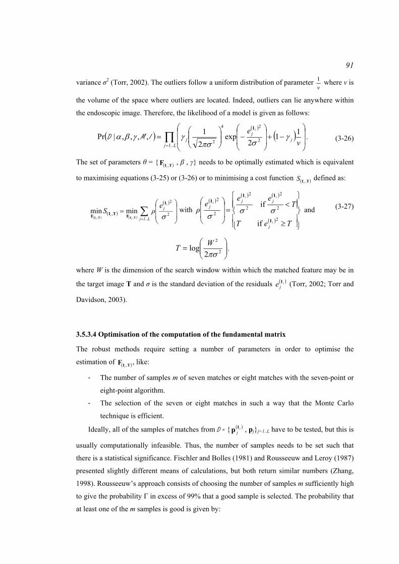
91
variance σ2 (Torr, 2002). The outliers follow a uniform distribution of parameter v1 where v is
the volume of the space where outliers are located. Indeed, outliers can lie anywhere within
the endoscopic image. Therefore, the likelihood of a model is given as follows:
( )( )
( )∏=
⎟⎟
⎠
⎞
⎜⎜
⎝
⎛−+⎟
⎟
⎠
⎞
⎜⎜
⎝
⎛−⎟⎟
⎠
⎞⎜⎜⎝
⎛=
Ljj
jj v
e i
..12
24
2
112
exp2
1,,,,|Pr γσπσ
γγβαI
IMD .
(3-26)
The set of parameters θ = { ( )TIF ,i , β , γ} needs to be optimally estimated which is equivalent
to maximising equations (3-25) or (3-26) or to minimising a cost function ( )TI ,iS defined as:
( )( )
( )
( )
∑=
⎟⎟
⎠
⎞
⎜⎜
⎝
⎛=
1..Lj
ji
ii
i
eρS 2
2
,,,
minminσ
I
FTIF TITI
with ( )
( ) ( )
( ) ⎪⎪⎭
⎪⎪⎬
⎫
⎪⎪⎩
⎪⎪⎨
⎧
≥
<=⎟
⎟
⎠
⎞
⎜⎜
⎝
⎛
TeT
Tee
eρ
i
ii
i
j
jjj
2
2
2
2
2
2
2
if
if
I
III
σσσ
and
⎟⎟⎠
⎞⎜⎜⎝
⎛= 2
2
2log
πσWT .
(3-27)
where W is the dimension of the search window within which the matched feature may be in
the target image T and σ is the standard deviation of the residuals ( )ije I (Torr, 2002; Torr and
Davidson, 2003).
3.5.3.4 Optimisation of the computation of the fundamental matrix
The robust methods require setting a number of parameters in order to optimise the
estimation of ( )TIF ,i, like:
- The number of samples m of seven matches or eight matches with the seven-point or
eight-point algorithm.
- The selection of the seven or eight matches in such a way that the Monte Carlo
technique is efficient.
Ideally, all of the samples of matches from D = { ( )ijIp , pj}j=1..L have to be tested, but this is
usually computationally infeasible. Thus, the number of samples needs to be set such that
there is a statistical significance. Fischler and Bolles (1981) and Rousseeuw and Leroy (1987)
presented slightly different means of calculations, but both return similar numbers (Zhang,
1998). Rousseeuw’s approach consists of choosing the number of samples m sufficiently high
to give the probability Γ in excess of 99% that a good sample is selected. The probability that
at least one of the m samples is good is given by:
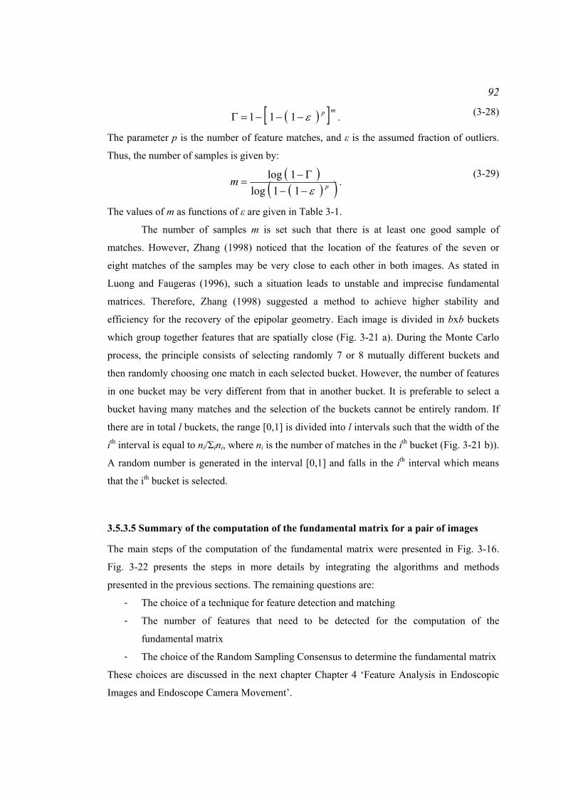
92
( )[ ]mpε−−−=Γ 111 . (3-28)
The parameter p is the number of feature matches, and ε is the assumed fraction of outliers.
Thus, the number of samples is given by:
( )( )( )pm
ε−−Γ−
=11log
1log.
(3-29)
The values of m as functions of ε are given in Table 3-1.
The number of samples m is set such that there is at least one good sample of
matches. However, Zhang (1998) noticed that the location of the features of the seven or
eight matches of the samples may be very close to each other in both images. As stated in
Luong and Faugeras (1996), such a situation leads to unstable and imprecise fundamental
matrices. Therefore, Zhang (1998) suggested a method to achieve higher stability and
efficiency for the recovery of the epipolar geometry. Each image is divided in bxb buckets
which group together features that are spatially close (Fig. 3-21 a). During the Monte Carlo
process, the principle consists of selecting randomly 7 or 8 mutually different buckets and
then randomly choosing one match in each selected bucket. However, the number of features
in one bucket may be very different from that in another bucket. It is preferable to select a
bucket having many matches and the selection of the buckets cannot be entirely random. If
there are in total l buckets, the range [0,1] is divided into l intervals such that the width of the
ith interval is equal to ni/Σini, where ni is the number of matches in the ith bucket (Fig. 3-21 b)).
A random number is generated in the interval [0,1] and falls in the ith interval which means
that the ith bucket is selected.
3.5.3.5 Summary of the computation of the fundamental matrix for a pair of images
The main steps of the computation of the fundamental matrix were presented in Fig. 3-16.
Fig. 3-22 presents the steps in more details by integrating the algorithms and methods
presented in the previous sections. The remaining questions are:
- The choice of a technique for feature detection and matching
- The number of features that need to be detected for the computation of the
fundamental matrix
- The choice of the Random Sampling Consensus to determine the fundamental matrix
These choices are discussed in the next chapter Chapter 4 ‘Feature Analysis in Endoscopic
Images and Endoscope Camera Movement’.

93
a) b) Fig. 3-21: The process of matches’ selection: a) the image is divided in buckets to group together the
features that are spatially close; b) the buckets are selected based on the number of features.
Table 3-1: Minimum number m of matches to draw for the estimation of the fundamental matrix:
Percentage of outliers
10% 20% 30% 40% 50% 60% 70% 80% 90%
m
for p = 7 8 20 54 163 588 2809 21 055 359 780 5x10⁷
m
for p = 8 9 26 78 272 1 177 7 025 70 188 1.8x10⁶ 4.6x10⁸
inputs Image IiImage T
Feature detection and matching with the LK tracker or the SIFT
Fundamental matrix computation:1. Translate and scale the coordinates of the features2. Apply the 7-point algorithm in a random sampling
consensus (LMedS, RANSAC, or MAPSAC):a. The features are drawn from 7 different bucketsb. The cost to minimise is a function of the Sampson’s
residuals3. Denormalise the first estimation of the fundamental matrix4. Refine this first estimation over the set of inliers by
constrained nonlinear optimisation
Correction of the endoscopic image distortionspreliminary step
F( , T)output
Ii Fig. 3-22: Summary of the framework and possible algorithms for the computation of the fundamental
matrix.
Image not displayed for Copyright reasons
94
3.6 Conclusion
Lesions detected by optical biopsy during gastroscopic, colonoscopic, or pulmonary
examinations can be re-localised using either pre-operative images and EM tracking systems,
or endoscopic images, or interventional MR images, or a combination of these modalities. A
clinical application of optical biopsies is the detection of biopsy sites invisible
macroscopically in the oesophagus during a surveillance examination of BO. Other
applications of optical biopsies can be the detection of flat polyps and microscopic colitis in
colon. These examinations make use of interventional endoscopic images. Thus, the re-
localisation of the lesions developed in this thesis for these clinical applications makes use of
endoscopic images only. The epipolar geometry formed by a reference image where the
biopsy site location is known and a target image where the biopsy site needs to be re-
localised has to be recovered for the specific case of the endoscopic images. The choice of the
algorithms is discussed in the next chapter.

95
Chapter 4 Feature Analysis in Endoscopic Images and
Endoscope Camera Movement
4.1 Introduction
The biopsy site is re-localised in a target endoscopic image T using the epipolar geometries
formed by this image with each reference image Ii. For each pair of images Ii ↔ T, the
epipolar geometry can be described algebraically by the fundamental matrix ( )TIF ,i. The
recovery of the epipolar geometry requires (Fig. 4-1):
- The correction of the distortions in the endoscopic images.
- The detection of features in the endoscopic images Ii and T and matching the features
together.
- The estimation of the fundamental matrix ( )TIF ,i from the set of matched features.
As the epipolar lines derived from the biopsy site locations in the reference images Ii
are used to re-localise the biopsy site in the target image T, they have to be computed with
high accuracy. This accuracy depends on:
- The number and proportion of good matched features termed inliers (Hartley and
Zisserman, 2004).
inputs Image I1Image T
Image IiImage T
Image INImage T
Feature detection and matching
Fundamental matrix computation
… …
Correction of the endoscopic image distortionspreliminary step
F( ,T)outputs F( ,T) F( ,T)I1 Ii IN Fig. 4-1: Framework for the estimation of the fundamental matrices that each reference image Ii forms
with the target image T.

96
- The wide spread of the features on the whole physical surface observed in the
endoscopic image (Luong and Faugeras, 1996).
- The method used to compute the fundamental matrix (Torr and Murray, 1997; Zhang,
1998; Torr and Zisserman, 2000; Hartley and Zisserman, 2004).
This chapter aims to present a method to compute an accurate fundamental matrix in
the specific context of endoscopic images. Methods for feature detection and matching are
discussed in this context. Algorithms for the recovery of the epipolar geometry as well as
their hypotheses are also discussed since their practical use can help determine which feature
detection and matching technique is well-adapted and how many features have to be detected
for the derivation of accurate epipolar lines.
4.2 Analysis of features in endoscopic images
Two main methods for feature detection and matching were presented in Chapter 3
‘Literature Review: Possible Approaches for Biopsy Site Re-localisation and Application for
the Surveillance Examination of Barrett’s Oesophagus’. These were the Lucas-Kanade (LK)
tracker which tracks features through endoscopic images and the Scale Invariant Feature
Transform which detects features independently in the images and which matches them using
their descriptors. The pros and cons of using these methods are discussed. Besides, the
algorithms used for the estimation of the fundamental matrix make the assumption that the
features are localised with an error that follows a Gaussian distribution. This assumption is
studied for the case of endoscopic images.
4.2.1 Feature detection in the image scale-space and matching of descriptors
The SIFT and the LK tracker have been used for feature detection and matching in
endoscopic images, for example by Mountney et al. (2006), Hu et al. (2007, 2009), and Luo
et al. (2010). The use of one method mainly depends on the type of sequences that need
processing.
SIFT feature matching has the advantage of detecting features independently in the
reference images and in the target image. Therefore, there is no tracking through consecutive
images to find the matches. The SIFT may be appropriate to sequences where intermediate
endoscopic images are blurred, or corrupted by the presence of air/water bubbles or by
specularities (Mori et al., 2005). Indeed, for this type of sequences, the LK tracker loses track
of the features and a method to start tracking again needs to be developed.
The neighbourhoods of the features that commonly correspond to vessel curvatures
and intersections look similar within an image and their visual content can change
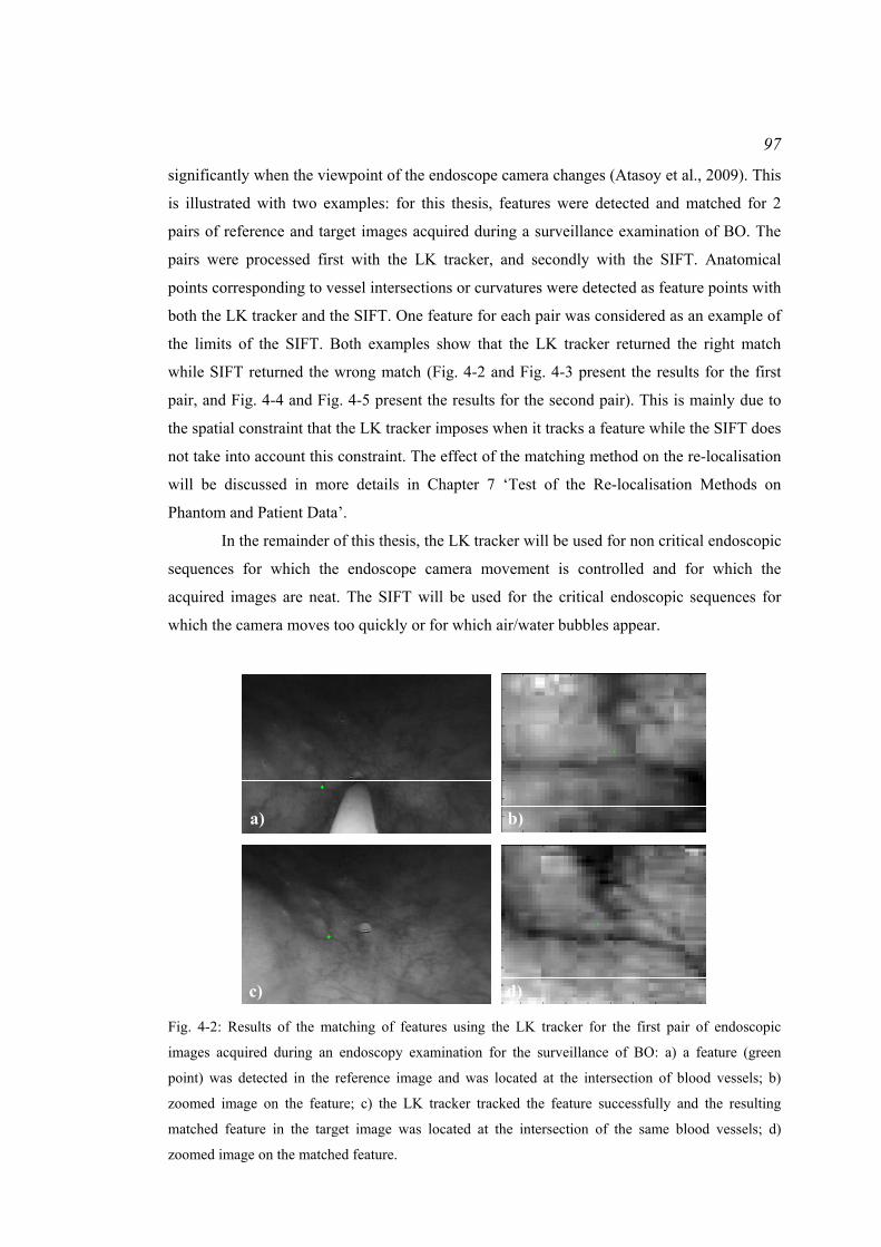
97
significantly when the viewpoint of the endoscope camera changes (Atasoy et al., 2009). This
is illustrated with two examples: for this thesis, features were detected and matched for 2
pairs of reference and target images acquired during a surveillance examination of BO. The
pairs were processed first with the LK tracker, and secondly with the SIFT. Anatomical
points corresponding to vessel intersections or curvatures were detected as feature points with
both the LK tracker and the SIFT. One feature for each pair was considered as an example of
the limits of the SIFT. Both examples show that the LK tracker returned the right match
while SIFT returned the wrong match (Fig. 4-2 and Fig. 4-3 present the results for the first
pair, and Fig. 4-4 and Fig. 4-5 present the results for the second pair). This is mainly due to
the spatial constraint that the LK tracker imposes when it tracks a feature while the SIFT does
not take into account this constraint. The effect of the matching method on the re-localisation
will be discussed in more details in Chapter 7 ‘Test of the Re-localisation Methods on
Phantom and Patient Data’.
In the remainder of this thesis, the LK tracker will be used for non critical endoscopic
sequences for which the endoscope camera movement is controlled and for which the
acquired images are neat. The SIFT will be used for the critical endoscopic sequences for
which the camera moves too quickly or for which air/water bubbles appear.
a) b)
c) d) Fig. 4-2: Results of the matching of features using the LK tracker for the first pair of endoscopic
images acquired during an endoscopy examination for the surveillance of BO: a) a feature (green
point) was detected in the reference image and was located at the intersection of blood vessels; b)
zoomed image on the feature; c) the LK tracker tracked the feature successfully and the resulting
matched feature in the target image was located at the intersection of the same blood vessels; d)
zoomed image on the matched feature.

98
a) b)
c) d)
e) f)
Fig. 4-3: Illustration of a mismatch with the SIFT for the first pair of endoscopic images acquired
during a surveillance examination of Barrett’s Oesophagus: a) a feature has been detected in the
reference image of the oesophagus at a given scale and with a given orientation: the feature is at the
centre of the circle whose radius is proportional to the scale of the feature and the drawn radius
indicates the orientation of the feature; b) zoomed image on the detected feature in a); c) the drawn
feature in the target image is the actual match of the feature drawn in a) but the matching process does
not match these two features; d) the zoomed image on the detected feature in c) shows that the
orientation of the feature is not the same as that of the feature in a); e) the matching process matches
the feature in a) with the feature in e) which does not correspond to the same anatomical point; f)
zoomed image on the feature detected in e).
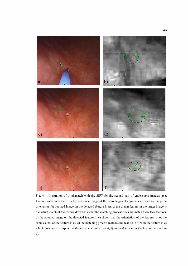
99
a) b)
c) d)
e) f) Fig. 4-4: Illustration of a mismatch with the SIFT for the second pair of endoscopic images: a) a
feature has been detected in the reference image of the oesophagus at a given scale and with a given
orientation; b) zoomed image on the detected feature in a); c) the drawn feature in the target image is
the actual match of the feature drawn in a) but the matching process does not match these two features;
d) the zoomed image on the detected feature in c) shows that the orientation of the feature is not the
same as that of the feature in a); e) the matching process matches the feature in a) with the feature in e)
which does not correspond to the same anatomical point; f) zoomed image on the feature detected in
e).
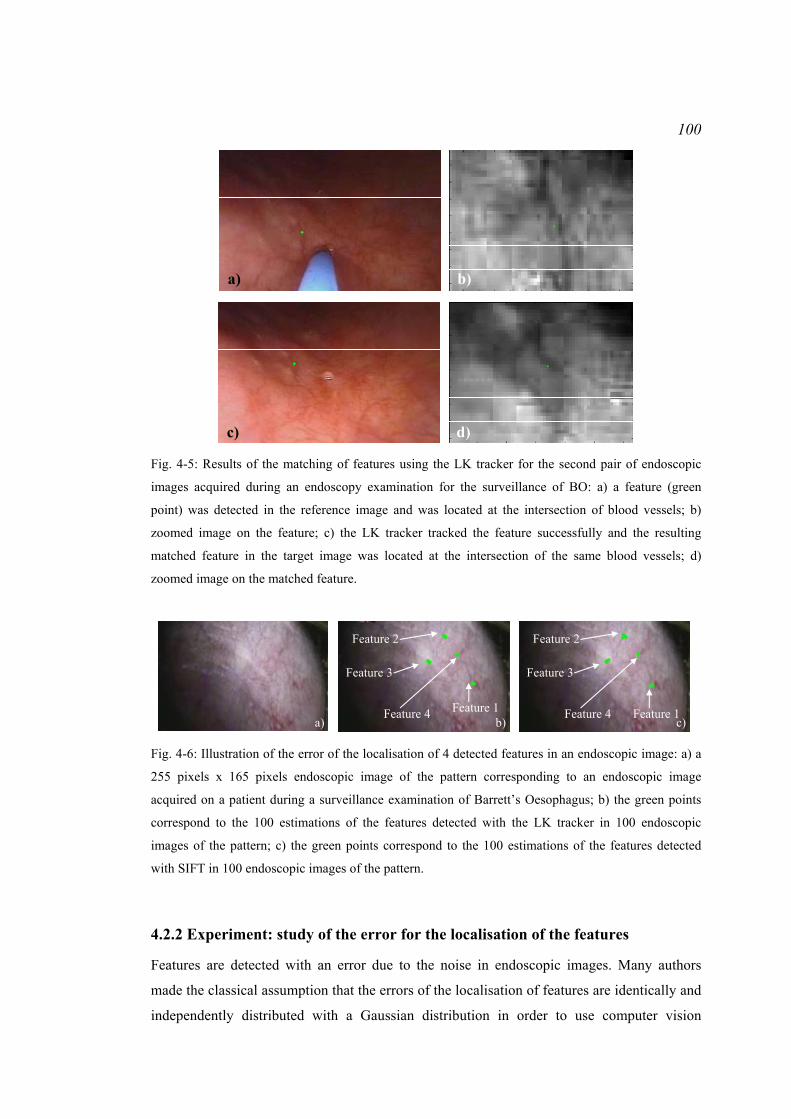
100
a) b)
c) d) Fig. 4-5: Results of the matching of features using the LK tracker for the second pair of endoscopic
images acquired during an endoscopy examination for the surveillance of BO: a) a feature (green
point) was detected in the reference image and was located at the intersection of blood vessels; b)
zoomed image on the feature; c) the LK tracker tracked the feature successfully and the resulting
matched feature in the target image was located at the intersection of the same blood vessels; d)
zoomed image on the matched feature.
Feature 1Feature 4
Feature 2
Feature 3
Feature 1Feature 4
Feature 2
Feature 3
a) b) c) Fig. 4-6: Illustration of the error of the localisation of 4 detected features in an endoscopic image: a) a
255 pixels x 165 pixels endoscopic image of the pattern corresponding to an endoscopic image
acquired on a patient during a surveillance examination of Barrett’s Oesophagus; b) the green points
correspond to the 100 estimations of the features detected with the LK tracker in 100 endoscopic
images of the pattern; c) the green points correspond to the 100 estimations of the features detected
with SIFT in 100 endoscopic images of the pattern.
4.2.2 Experiment: study of the error for the localisation of the features
Features are detected with an error due to the noise in endoscopic images. Many authors
made the classical assumption that the errors of the localisation of features are identically and
independently distributed with a Gaussian distribution in order to use computer vision
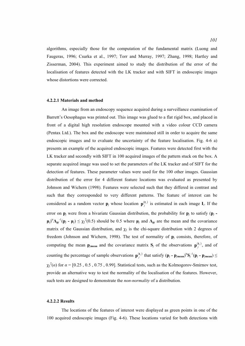
101
algorithms, especially those for the computation of the fundamental matrix (Luong and
Faugeras, 1996; Csurka et al., 1997; Torr and Murray, 1997; Zhang, 1998; Hartley and
Zisserman, 2004). This experiment aimed to study the distribution of the error of the
localisation of features detected with the LK tracker and with SIFT in endoscopic images
whose distortions were corrected.
4.2.2.1 Materials and method
An image from an endoscopy sequence acquired during a surveillance examination of
Barrett’s Oesophagus was printed out. This image was glued to a flat rigid box, and placed in
front of a digital high resolution endoscope mounted with a video colour CCD camera
(Pentax Ltd.). The box and the endoscope were maintained still in order to acquire the same
endoscopic images and to evaluate the uncertainty of the feature localisation. Fig. 4-6 a)
presents an example of the acquired endoscopic images. Features were detected first with the
LK tracker and secondly with SIFT in 100 acquired images of the pattern stuck on the box. A
separate acquired image was used to set the parameters of the LK tracker and of SIFT for the
detection of features. These parameter values were used for the 100 other images. Gaussian
distribution of the error for 4 different feature locations was evaluated as presented by
Johnson and Wichern (1998). Features were selected such that they differed in contrast and
such that they corresponded to very different patterns. The feature of interest can be
considered as a random vector pj whose location ( )ijIp is estimated in each image Ii. If the
error on pj were from a bivariate Gaussian distribution, the probability for pj to satisfy (pj -
μj)trΛpj-1(pj - μj) ≤ χ2
2(0.5) should be 0.5 where μj and Λpj are the mean and the covariance
matrix of the Gaussian distribution, and χ2 is the chi-square distribution with 2 degrees of
freedom (Johnson and Wichern, 1998). The test of normality of pj consists, therefore, of
computing the mean pjmean and the covariance matrix Sj of the observations ( )ijIp , and of
counting the percentage of sample observations ( )ijIp that satisfy (pj - pjmean)trSj
-1(pj - pjmean) ≤
χ22(α) for α = [0.25 , 0.5 , 0.75 , 0.99]. Statistical tests, such as the Kolmogorov-Smirnov test,
provide an alternative way to test the normality of the localisation of the features. However,
such tests are designed to demonstrate the non-normality of a distribution.
4.2.2.2 Results
The locations of the features of interest were displayed as green points in one of the
100 acquired endoscopic images (Fig. 4-6). These locations varied for both detections with
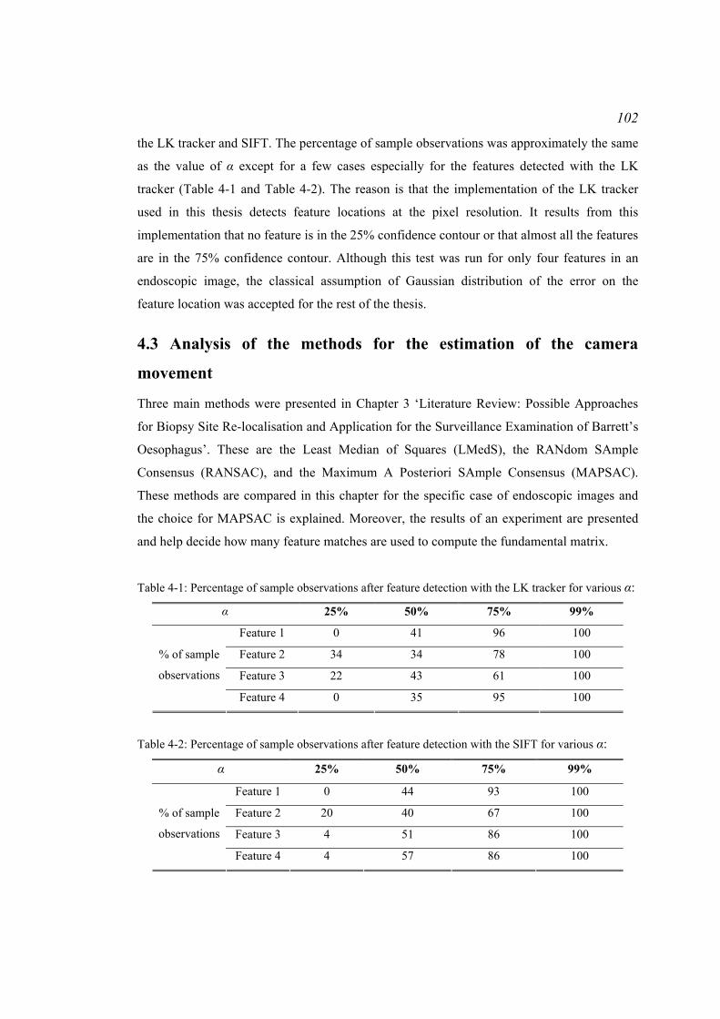
102
the LK tracker and SIFT. The percentage of sample observations was approximately the same
as the value of α except for a few cases especially for the features detected with the LK
tracker (Table 4-1 and Table 4-2). The reason is that the implementation of the LK tracker
used in this thesis detects feature locations at the pixel resolution. It results from this
implementation that no feature is in the 25% confidence contour or that almost all the features
are in the 75% confidence contour. Although this test was run for only four features in an
endoscopic image, the classical assumption of Gaussian distribution of the error on the
feature location was accepted for the rest of the thesis.
4.3 Analysis of the methods for the estimation of the camera
movement
Three main methods were presented in Chapter 3 ‘Literature Review: Possible Approaches
for Biopsy Site Re-localisation and Application for the Surveillance Examination of Barrett’s
Oesophagus’. These are the Least Median of Squares (LMedS), the RANdom SAmple
Consensus (RANSAC), and the Maximum A Posteriori SAmple Consensus (MAPSAC).
These methods are compared in this chapter for the specific case of endoscopic images and
the choice for MAPSAC is explained. Moreover, the results of an experiment are presented
and help decide how many feature matches are used to compute the fundamental matrix.
Table 4-1: Percentage of sample observations after feature detection with the LK tracker for various α:
α 25% 50% 75% 99%
Feature 1 0 41 96 100
Feature 2 34 34 78 100
Feature 3 22 43 61 100
% of sample
observations
Feature 4 0 35 95 100
Table 4-2: Percentage of sample observations after feature detection with the SIFT for various α:
α 25% 50% 75% 99%
Feature 1 0 44 93 100
Feature 2 20 40 67 100
Feature 3 4 51 86 100
% of sample
observations
Feature 4 4 57 86 100

103
4.3.1 Experiment: comparison of the estimations of the fundamental matrix with
LMedS, RANSAC, and MAPSAC
Torr and Murray (1997) and Torr (2002) investigated the performances of the LMedS,
RANSAC, and MAPSAC methods. They found that the MAPSAC outperformed the other
two methods as it searches for the fundamental matrix ( )TIF ,i which best fits the set of
detected inliers while the other two methods tend to return the solution which maximises the
number of inliers. The following experiment also illustrates why the MAPSAC is chosen for
the recovery of the epipolar geometry between endoscopic images.
4.3.1.1 Materials and method
The overall goal of the biopsy site re-localisation is the determination of accurate
epipolar lines. Therefore, this experiment compared the accuracy of the epipolar lines in the
target image T derived from the biopsy site location in the reference images Ii with the 3
methods LMedS, RANSAC, and MAPSAC. The epipolar geometry was recovered by
following the process presented in Fig. 3-22. One sequence from the same surveillance
examination of Barrett’s Oesophagus (BO) of a patient was processed. Image dimensions
were 339 pixels x 216 pixels and the sequence included 101 images. Images were
undistorted.
The first image was used to tune the parameters for feature detection and tracking
with the LK tracker. The number of inliers was counted which helped set the number m of
repeats of the random sampling consensus for the computation of the fundamental matrix.
The fundamental matrix was recovered between this first image and the last image of the
sequence with the LMedS in order to find an estimate of the residuals ( )ije I and of their
standard deviation σ. This standard deviation was used to set the threshold T for the
distinction of inliers and outliers with RANSAC and MAPSAC. Given the image dimensions,
the size of the buckets to group the features that are spatially close was set at 20 pixels.
For the 100 other pairs of images Ii ↔ T:
- The feature matches were found with the LK tracker
- The fundamental matrices were recovered, afterwards, with either the LMedS, or the
RANSAC, or the MAPSAC.
Table 4-3: RMS errors in pixels of the distances from the epipolar lines to the ground-truth of the
biopsy site in the target image T when the lines are computed with LMedS, RANSAC, or MAPSAC:
RMSLMedS (pixels) RMSRANSAC (pixels) RMSMAPSAC (pixels)
1.86 1.80 1.70
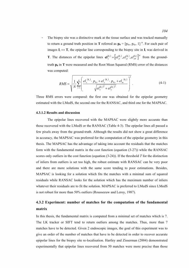
104
- The biopsy site was a distinctive mark at the tissue surface and was tracked manually
to return a ground truth position in T referred as p0 = [p0x, p0y, 1] tr. For each pair of
images Ii ↔ T, the epipolar line corresponding to the biopsy site in Ii was derived in
T. The distances of the epipolar lines ( ) ( ) ( ) ( )[ ] tr,, iiii
jmjyjxj elelel IIIIel = from the ground-
truth p0 in T were measured and the Root Mean Squared (RMS) error of the distances
was computed:
( ) ( ) ( )
( ) ( )∑= ⎟
⎟⎟
⎠
⎞
⎜⎜⎜
⎝
⎛
+
+⋅+⋅=
N
iyx
myyxx
ii
iii
elel
elpelpelN
RMS1
2
22
001II
III
.
(4-1)
Three RMS errors were compared: the first one was obtained for the epipolar geometry
estimated with the LMedS, the second one for the RANSAC, and third one for the MAPSAC.
4.3.1.2 Results and discussion
The epipolar lines recovered with the MAPSAC were slightly more accurate than
those recovered with the LMedS or the RANSAC (Table 4-3). The epipolar lines all passed a
few pixels away from the ground-truth. Although the results did not show a great difference
in accuracy, the MAPSAC was preferred for the computation of the epipolar geometry in this
thesis. The MAPSAC has the advantage of taking into account the residuals that the matches
form with the fundamental matrix in the cost function (equation (3-27)) while the RANSAC
scores only outliers in the cost function (equation (3-24)). If the threshold T for the distinction
of inliers from outliers is set too high, the robust estimate with RANSAC can be very poor
and there are more solutions with the same score tending to poor estimations. Besides,
MAPSAC is looking for a solution which fits the matches with a minimal sum of squared
residuals while RANSAC looks for the solution which has the maximum number of inliers
whatever their residuals are to fit the solution. MAPSAC is preferred to LMedS since LMedS
is not robust for more than 50% outliers (Rousseeuw and Leroy, 1987).
4.3.2 Experiment: number of matches for the computation of the fundamental
matrix
In this thesis, the fundamental matrix is computed from a minimal set of matches which is 7.
The LK tracker or SIFT tend to return outliers among the matches. Thus, more than 7
matches have to be detected. Given 2 endoscopic images, the goal of this experiment was to
give an order of the number of matches that have to be detected in order to recover accurate
epipolar lines for the biopsy site re-localisation. Hartley and Zisserman (2004) demonstrated
experimentally that epipolar lines recovered from 50 matches were more precise than those
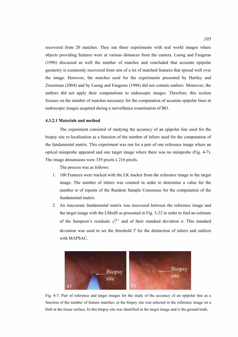
105
recovered from 20 matches. They ran these experiments with real world images where
objects providing features were at various distances from the camera. Luong and Faugeras
(1996) discussed as well the number of matches and concluded that accurate epipolar
geometry is commonly recovered from sets of a lot of matched features that spread well over
the image. However, the matches used for the experiments presented by Hartley and
Zisserman (2004) and by Luong and Faugeras (1996) did not contain outliers. Moreover, the
authors did not apply their computations to endoscopic images. Therefore, this section
focuses on the number of matches necessary for the computation of accurate epipolar lines in
endoscopic images acquired during a surveillance examination of BO.
4.3.2.1 Materials and method
The experiment consisted of studying the accuracy of an epipolar line used for the
biopsy site re-localisation as a function of the number of inliers used for the computation of
the fundamental matrix. This experiment was run for a pair of one reference image where an
optical miniprobe appeared and one target image where there was no miniprobe (Fig. 4-7).
The image dimensions were 339 pixels x 216 pixels.
The process was as follows:
1. 100 Features were tracked with the LK tracker from the reference image to the target
image. The number of inliers was counted in order to determine a value for the
number m of repeats of the Random Sample Consensus for the computation of the
fundamental matrix.
2. An inaccurate fundamental matrix was recovered between the reference image and
the target image with the LMedS as presented in Fig. 3-22 in order to find an estimate
of the Sampson’s residuals ( )ije I and of their standard deviation σ. This standard
deviation was used to set the threshold T for the distinction of inliers and outliers
with MAPSAC.
a) b)
Biopsy site
Biopsy site
Fig. 4-7: Pair of reference and target images for the study of the accuracy of an epipolar line as a
function of the number of feature matches: a) the biopsy site was selected in the reference image on a
blob at the tissue surface, b) this biopsy site was identified in the target image and is the ground truth.

106 Table 4-4: Accuracy of the epipolar line as a function of the number of matches in the pair of reference
image and target image.
Bucket size (pixels) 8 10 12 15 20 25 30 35
Number of matches 98 86 63 43 32 27 16 15
Number of inliers detected by MAPSAC
66 55 40 27 20 17 10 8
Accuracy (pixels) -1.39 -1.22 -4.71 6.21 7.31 6.61 22.01 -23.94
3. The features were grouped into buckets as described in section ‘3.5.3.4 Optimisation
of the computation of the fundamental matrix’. The bucket size took the values as
follows: 8, 10, 12, 15, 20, 25, 30, and 35 pixels. For each bucket size, the
fundamental matrix was computed as presented in Fig. 3-22 using MAPSAC and the
values of m and T found in steps 1 and 2. The size of the bucket was, therefore, used
to control the number of matches and to guarantee a good spread of the features over
the whole 3D surface observed with the endoscope camera.
4. A point was selected manually in the reference image and tracked manually in the
target image to be the biopsy site. This biopsy site corresponded to a salient blob well
identified in these images. The location of the biopsy site in the target image was the
ground truth and noted p0 = [p0x, p0y, 1] tr. After the computation of the fundamental
matrix for each bucket size, the epipolar line el = [elx, ely, elm] tr was derived in the
target image from the biopsy site location in the reference image. The accuracy of the
epipolar line was measured in pixels as the distance from the epipolar line to the
ground truth in the target image:
22
00accuracyyx
myyxx
elel
elpelpel
+
+⋅+⋅= .
(4-2)
4.3.2.2 Results and discussion
Approximately 30% outliers were detected manually during the counting process.
According to Table 3-1, only 54 tests of the MAPSAC could be applied to compute a correct
fundamental matrix. However, in order to improve the chance to compute an accurate
fundamental matrix, 3000 tests were run. When the number of matches was high which
corresponded to small bucket sizes, for example 63, 86, or 98, the epipolar line was accurate
(Table 4-4). The corresponding fundamental matrices were recovered from a high number of
inliers, respectively 40, 55, and 66. For fewer matches, the accuracy was getting worse. For

107
these cases, outliers corrupted the sets of matches and the fundamental matrix could have
been wrongly computed by detecting an outlier as an inlier. Thus, in practice for the rest of
this thesis, the LK tracker and the SIFT were tuned such that approximately 100 matches
could be detected.
4.4 Conclusion
This chapter discussed the method to recover accurate epipolar geometry for the pairs of
reference images Ii and target image T where the re-localised biopsy site needs to be
computed. In practice, sequences were processed offline after the endoscopy examination.
Before the examination and image acquisition, the endoscope camera was calibrated in order
to estimate the barrel distortions. Each acquired sequence was corrected for distortions after
the examination. A sequence refers to a series of images acquired around the detected biopsy
site. The last image of the sequence was used as the target image where the biopsy site
needed to be re-localised. The first image of the sequence was used to tune the parameters of
the algorithms for feature detection and matching and for epipolar geometry recovery.
For the tuning, features were preferably detected and matched with the LK tracker
applied to the first image of the sequence and to the target image. The LK tracker failed when
the endoscope camera moved too quickly and generated blurred images, or when air/water
bubbles obstructed the camera field of view. In these cases, SIFT features were detected and
matched, but the matching could generate a great number of outliers since it does not impose
a spatial constraint. Approximately 100 matches could be detected. The number of outliers
was counted visually in order to set the number of estimations necessary for the estimation of
the epipolar geometry. The epipolar geometry was recovered using a combination of the 7-
point algorithm with the LMedS. The 7-point algorithm was used since it imposes the
constraint that the determinant of ( )TIF ,i is null. The LMedS was used in order to estimate the
standard deviation of the Sampson’s residuals that the matches formed with the estimated
fundamental matrix. Features in the training image and in the target image were grouped in
buckets. For images whose dimensions were of the order of 200 pixels x 200 pixels, the
dimensions of the buckets were 20 pixels x 20 pixels.
The other endoscopic images were processed after parameter tuning. Features were
detected and matched using the LK tracker or SIFT. The 7-point algorithm was run in
combination with MAPSAC in order to estimate the epipolar geometries. The number of tests
for MAPSAC was set at 3000 in order to guarantee a great chance of computing accurate
fundamental matrix. Features in the images were grouped within buckets as for the tuning
step.

108
The next chapters demonstrate how accurate epipolar lines can be used to re-localise
the biopsy site accurately and precisely, and to determine the confidence of the re-
localisation. Moreover, another chapter presents a method to improve the accuracy of the
epipolar lines when they are recovered from SIFT matches.
109
Chapter 5 Re-localisation of Biopsy Sites during Endoscopy
Examinations
5.1 Introduction
Biopsy sites detected by optical biopsy during a surveillance examination of Barrett’s
Oesophagus (BO) need to be re-localised in the endoscopic images acquired during the same
examination in order to guide instruments to the biopsy sites for tissue excision, or for
treatment, or for a new tissue interrogation by optical biopsy.
The approach for the biopsy site re-localisation is based on the computation of the
mapping from one reference image Ii where the biopsy site location is known to the target
image T. In the previous chapters, it was shown that this mapping can be the fundamental
matrix ( )TIF ,i which is estimated during the recovery of the epipolar geometry formed by the
pair of images Ii ↔ T. In order to recover the epipolar geometry, features in both images
need to be detected and matched, which can be done with the Lucas Kanade (LK) tracker or
with the Scale Invariant Feature Transform (SIFT). Bad matches due to failures of the LK
tracker or the SIFT corrupt the accuracy of the epipolar geometry. They are, therefore,
detected when ( )TIF ,i is estimated. The Maximum A Posteriori Sample Consensus (MAPSAC)
finds a first estimate of ( )TIF ,i that fits best the set of inliers or good feature matches. The
estimated ( )TIF ,i is refined by non-linear optimisation over the whole set of detected inliers.
The fundamental matrix ( )TIF ,i transforms a point of the reference image Ii in a line
termed epipolar line in the target image T. This line indicates the locus of the image point in
T. In this chapter, a method is presented to re-localise the biopsy site in T using epipolar
lines. Either 2 epipolar lines or N > 2 epipolar lines are used for the re-localisation. This was
first published in Allain et al. (2009a.) and in Allain et al. (2010). The results of studies of the
influence on the re-localised biopsy site of the accuracy of the epipolar lines and of the angles
they subtend are discussed in this chapter.
5.2 Re-localisation principle
Epipolar lines derived from the biopsy site in the reference images Ii indicate a direction in
the target image T along which the biopsy site is. Geometric information from the epipolar
lines can be combined in order to determine the location of the biopsy site in T.
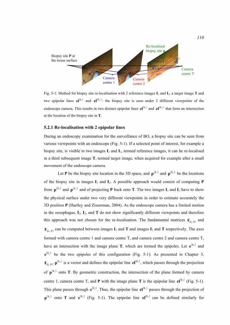
110
Biopsy site P at the tissue surface
Camera centre 1
Camera centre T
I1TI2
Camera centre 2
Re-localised biopsy site p
pp
e
e(I2)
elel
(I1)
(I1)
(I 1)
(I2)
(I 2)
Fig. 5-1: Method for biopsy site re-localisation with 2 reference images I1 and I2, a target image T and
two epipolar lines ( )1Iel and ( )2Iel : the biopsy site is seen under 2 different viewpoints of the
endoscope camera. This results in two distinct epipolar lines ( )1Iel and ( )2Iel that form an intersection
at the location of the biopsy site in T.
5.2.1 Re-localisation with 2 epipolar lines
During an endoscopy examination for the surveillance of BO, a biopsy site can be seen from
various viewpoints with an endoscope (Fig. 5-1). If a selected point of interest, for example a
biopsy site, is visible in two images I1 and I2, termed reference images, it can be re-localised
in a third subsequent image T, termed target image, when acquired for example after a small
movement of the endoscope camera.
Let P be the biopsy site location in the 3D space, and ( )1Ip and ( )2Ip be the locations
of the biopsy site in images I1 and I2. A possible approach would consist of computing P
from ( )1Ip and ( )2Ip and of projecting P back onto T. The two images I1 and I2 have to show
the physical surface under two very different viewpoints in order to estimate accurately the
3D position P (Hartley and Zisserman, 2004). As the endoscope camera has a limited motion
in the oesophagus, I1, I2, and T do not show significantly different viewpoints and therefore
this approach was not chosen for the re-localisation. The fundamental matrices ( )TIF ,1 and
( )TIF ,2 can be computed between images I1 and T and images I2 and T respectively. The axes
formed with camera centre 1 and camera centre T, and camera centre 2 and camera centre T,
have an intersection with the image plane T, which are termed the epipoles. Let ( )1Ie and ( )2Ie be the two epipoles of this configuration (Fig. 5-1). As presented in Chapter 3,
( )TIF ,1. ( )1Ip is a vector and defines the epipolar line ( )1Iel , which passes through the projection
of ( )1Ip onto T. By geometric construction, the intersection of the plane formed by camera
centre 1, camera centre T, and P with the image plane T is the epipolar line ( )1Iel (Fig. 5-1).
This plane passes through ( )1Ie . Thus, the epipolar line ( )1Iel passes through the projection of ( )1Ip onto T and ( )1Ie (Fig. 5-1). The epipolar line ( )2Iel can be defined similarly for

111
( )TIF ,2. ( )2Ip . The two epipolar lines indicate the locus of the possible images of ( )1Ip and
( )2Ip . As ( )1Ip and ( )2Ip correspond to the same biopsy site location in the 3D-space, the
intersection of ( )1Iel and ( )2Iel returns the location of the biopsy site in the target image T
(Allain et al., 2009a). A similar method was first proposed by Faugeras and Robert (1994).
However, they applied it to real world images representing the same object seen under
various viewpoints without the presence of instruments obstructing the camera field of view
and positioned at various locations in several images.
During endoscopy, the biopsy site location is defined and issued at that point imaged
with an optical biopsy miniprobe passed via the working channel of the endoscope. The
imaging axis is commonly arranged around the central axis of the endoscope. Thus, twisting
the head of the endoscope creates rotations and translations of the camera, while the probe
remains at its location at the tissue surface. This motion helps generate different views of the
biopsy site and different epipolar lines can be derived.
5.2.2 Limits of the re-localisation with 2 epipolar lines due to their uncertainty
The epipolar geometry formed by the pair of reference image Ii and target image T is
recovered from a set of matched features D = { ( )ijIp , pj}j=1..L with ( ) ( ) ( )[ ] tr
1,, iiijyjxj pp IIIp = , a
feature in Ii which matches pj = [pjx, pjy, 1] tr, a feature in T. The endoscopes that were used
for this thesis were mounted with a CCD camera. Noise appears in the images acquired with
a CCD camera and has an influence on the detection of features, on the determination of their
locations, and propagates to the fundamental matrix ( )TIF ,i and to the epipolar lines ( )iIel .
As stated in Chapter 4, Section 4.2.2 Experiment: study of the error for the
localisation of the features’), the features ( )ijIp and pj detected with the LK tracker or with the
SIFT are localised with an error. Many authors assumed that the errors of the localisations of
features ( )ijIp are identically and independently distributed with a Gaussian distribution and
they approximated the covariance matrix of these errors as ( )ijIp
Λ = σ12 where 12 is the 2x2
identity matrix (Luong and Faugeras, 1996; Csurka et al., 1997; Torr and Murray, 1997;
Zhang, 1998; Hartley and Zisserman, 2004). The experiments in Chapter 4 section ‘4.2.2
Experiment: study of the error for the localisation of the features’ confirmed that this is a
reasonable model for the images acquired with an endoscope and for the features extracted
with the LK tracker or with the SIFT.
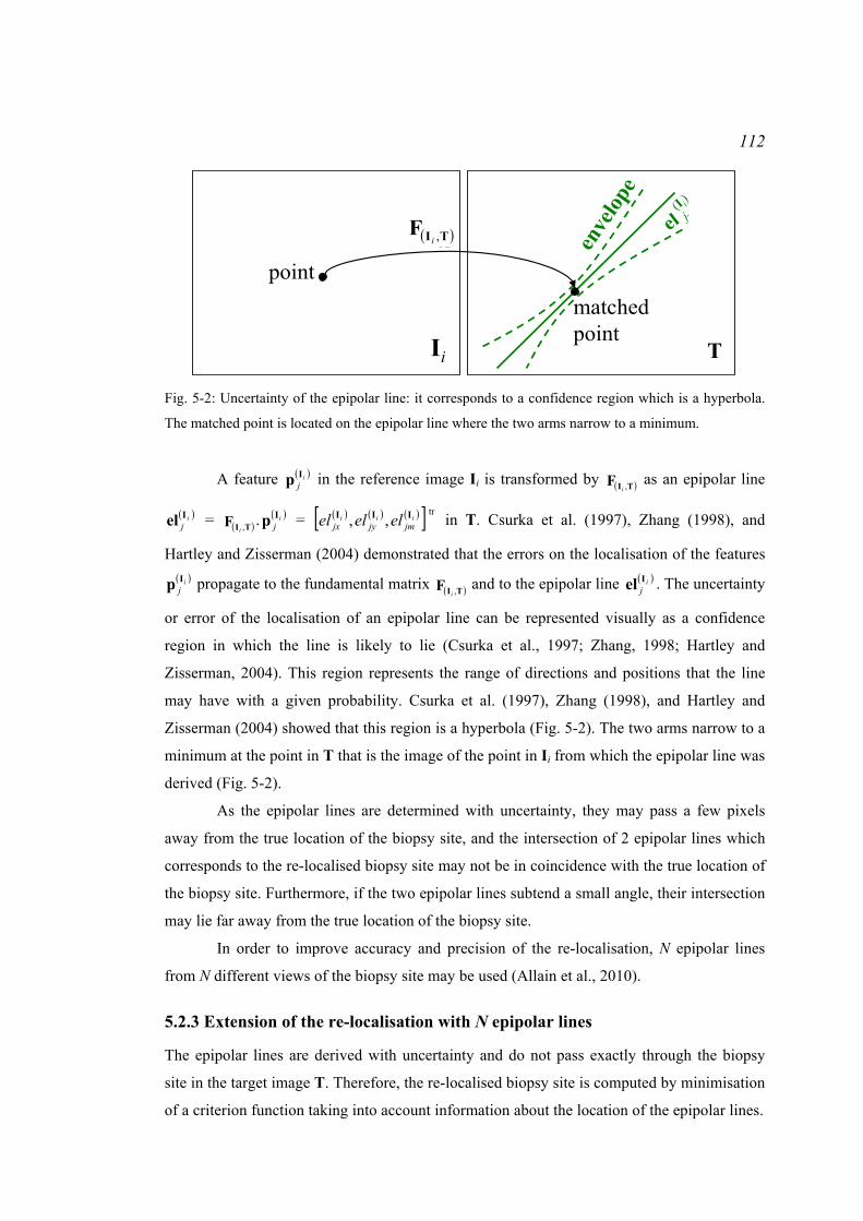
112
matchedpoint
Ii
point
T
el i
enve
lope
FiT
Ii
( )TIF ,iel
(I i)j
Fig. 5-2: Uncertainty of the epipolar line: it corresponds to a confidence region which is a hyperbola.
The matched point is located on the epipolar line where the two arms narrow to a minimum.
A feature ( )ijIp in the reference image Ii is transformed by ( )TIF ,i
as an epipolar line
( )ijIel = ( )TIF ,i
. ( )ijIp = ( ) ( ) ( )[ ] tr
,, iiijmjyjx elelel III in T. Csurka et al. (1997), Zhang (1998), and
Hartley and Zisserman (2004) demonstrated that the errors on the localisation of the features ( )ijIp propagate to the fundamental matrix ( )TIF ,i
and to the epipolar line ( )ijIel . The uncertainty
or error of the localisation of an epipolar line can be represented visually as a confidence
region in which the line is likely to lie (Csurka et al., 1997; Zhang, 1998; Hartley and
Zisserman, 2004). This region represents the range of directions and positions that the line
may have with a given probability. Csurka et al. (1997), Zhang (1998), and Hartley and
Zisserman (2004) showed that this region is a hyperbola (Fig. 5-2). The two arms narrow to a
minimum at the point in T that is the image of the point in Ii from which the epipolar line was
derived (Fig. 5-2).
As the epipolar lines are determined with uncertainty, they may pass a few pixels
away from the true location of the biopsy site, and the intersection of 2 epipolar lines which
corresponds to the re-localised biopsy site may not be in coincidence with the true location of
the biopsy site. Furthermore, if the two epipolar lines subtend a small angle, their intersection
may lie far away from the true location of the biopsy site.
In order to improve accuracy and precision of the re-localisation, N epipolar lines
from N different views of the biopsy site may be used (Allain et al., 2010).
5.2.3 Extension of the re-localisation with N epipolar lines
The epipolar lines are derived with uncertainty and do not pass exactly through the biopsy
site in the target image T. Therefore, the re-localised biopsy site is computed by minimisation
of a criterion function taking into account information about the location of the epipolar lines.

113
The re-localised biopsy site p in the target image T must satisfy the condition of
triangulation with its match ( )iIp in the reference image Ii (Hartley, 1997). This condition
means that the two axes passing respectively through Camera centre i and ( )iIp , and through
Camera centre T and p, must meet at the position of the biopsy site P in the 3D space (Fig.
5-3). Longuet-Higgins (1981) demonstrated that the two axes corresponding to the matching
pair of points ( )iIp ↔ p will meet in space if and only if the algebraic residual that the points
form with the fundamental matrix is null:
( )( ) 0,
tr =⋅⋅ i
i
ITI pFp . (5-1)
As discussed in section ‘5.2.2 Limits of the re-localisation with 2 epipolar lines due to their
uncertainty’, the fundamental matrix ( )TIF ,i is determined with uncertainty. Given the biopsy
site location ( )iIp in the reference image Ii and its image p in the target image T, the
algebraic residual for the pair of points ( )iIp ↔ p is not null. Therefore, the re-localised
biopsy site p can be computed by minimisation of the algebraic residuals with the least
squares method (Bjorck, 1996):
( )( )( )∑
=
⋅⋅N
i
i1
2,
trmini
ITIp
pFp . (5-2)
Minimising the sum of squared algebraic residuals may not return a good estimation
of the re-localised biopsy site p:
− Torr (1995), Hartley and Zisserman (2004), and Hu et al. (2008b) stated that the
algebraic residual does not have a geometric meaning. A better measure to minimise is the
perpendicular distance from the feature matches to the fitting ellipse that corresponds to the
fundamental matrix.
Biopsy site P at the tissue surface
Camera centre i
Camera centre T
IiT
Re-localised biopsy site pF( ,T)
el
ep(Ii)
Ii
(I i)
(Ii)
Fig. 5-3: Condition of triangulation: the two axes passing respectively through Camera centre i and
( )iIp , and through Camera centre T and p, must meet at the position of the biopsy site P in the 3D
space.
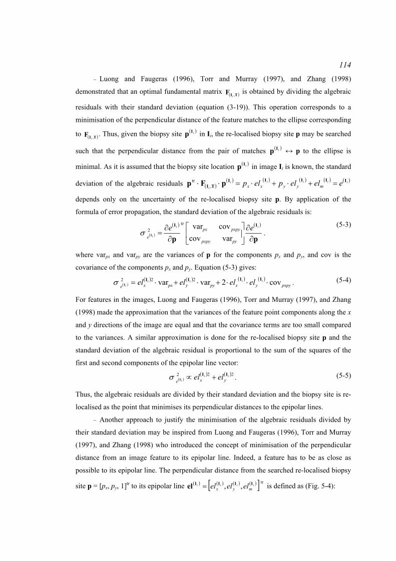
114
− Luong and Faugeras (1996), Torr and Murray (1997), and Zhang (1998)
demonstrated that an optimal fundamental matrix ( )TIF ,i is obtained by dividing the algebraic
residuals with their standard deviation (equation (3-19)). This operation corresponds to a
minimisation of the perpendicular distance of the feature matches to the ellipse corresponding
to ( )TIF ,i. Thus, given the biopsy site ( )iIp in Ii, the re-localised biopsy site p may be searched
such that the perpendicular distance from the pair of matches ( )iIp ↔ p to the ellipse is
minimal. As it is assumed that the biopsy site location ( )iIp in image Ii is known, the standard
deviation of the algebraic residuals ( )( ) ( ) ( ) ( ) ( )iiiii
ieelelpelp myyxx
IIIIITI pFp =+⋅+⋅=⋅⋅ ,
tr
depends only on the uncertainty of the re-localised biopsy site p. By application of the
formula of error propagation, the standard deviation of the algebraic residuals is:
( )
( ) ( )
pp
II
I∂∂
⎥⎦
⎤⎢⎣
⎡∂∂
=ii
i
eepypxpy
pxpypx
e varcovcovvartr
2σ . (5-3)
where varpx and varpy are the variances of p for the components px and py, and cov is the
covariance of the components px and py. Equation (5-3) gives:
( )( ) ( ) ( ) ( )
pxpyyxpyypxxeiiii
i elelelel cov2varvar 222 ⋅⋅⋅+⋅+⋅= IIIIIσ . (5-4)
For features in the images, Luong and Faugeras (1996), Torr and Murray (1997), and Zhang
(1998) made the approximation that the variances of the feature point components along the x
and y directions of the image are equal and that the covariance terms are too small compared
to the variances. A similar approximation is done for the re-localised biopsy site p and the
standard deviation of the algebraic residual is proportional to the sum of the squares of the
first and second components of the epipolar line vector:
( )( ) ( )222 ii
i yxeelel II
I +∝σ . (5-5)
Thus, the algebraic residuals are divided by their standard deviation and the biopsy site is re-
localised as the point that minimises its perpendicular distances to the epipolar lines.
− Another approach to justify the minimisation of the algebraic residuals divided by
their standard deviation may be inspired from Luong and Faugeras (1996), Torr and Murray
(1997), and Zhang (1998) who introduced the concept of minimisation of the perpendicular
distance from an image feature to its epipolar line. Indeed, a feature has to be as close as
possible to its epipolar line. The perpendicular distance from the searched re-localised biopsy
site p = [px, py, 1]tr to its epipolar line ( ) ( ) ( ) ( )[ ] tr,, iiii
myx elelel IIIIel = is defined as (Fig. 5-4):

115
( )( )( ) ( ) ( )
( ) ( )
( )( )
( )( )( ) ( )
( )( ) 2
2,2
1,
,tr
22,
i
i
i
i
i
i
ii
iii
i
yx
myyxx
elel
elpelpeld
ITI
ITI
ITI
II
IIII
pFpF
pFp
elp
⋅+⋅
⋅⋅=
+
+⋅+⋅=
.
(5-6)
where ( ( )TIF ,i. ( )iIp )1 = ( )i
xel I is the first component of the vector ( )TIF ,i. ( )iIp . This distance is a
signed measure.
For these three reasons, the re-localised biopsy site p in the target image T is
computed such that it minimises by the linear least squares method the sum of all of its
distances from the epipolar lines { ( )iIel }i=1..N:
( ) ( )( ) ( )( )∑∑==
===N
i
N
ii
ii dCCC1
2
1
2min ,min,minmin I
p
I
ppelpelpp .
(5-7)
el(If)
el (In)
el(Iw)
el(I f)
el (In )
el(Iw)
Fig. 5-4: The definition of the re-localised biopsy site p: it is defined such that it minimises the sum of
the perpendicular distances to the epipolar lines.
inputs
output
Image I1Image T
Image IiImage T
Image INImage T
Feature detection and matching
Fundamental matrix computation
- If N = 2, p is at the intersection of the two epipolar lines- If N > 2, solve for p such that it minimises the sum of its perpendicular distances to the epipolar lines
Re-localised biopsy site p
… …
Correction of the endoscopic image distortionspreliminary step
Fig. 5-5: Framework for the biopsy site re-localisation in the target image T.

116
C is the cost function to minimise. This solution makes the assumption that no epipolar line
in { ( )iIel }i=1..N is an outlier. This assumption is valid since the epipolar geometries formed for
each pair of reference and target images Ii ↔ T are computed initially from sets of inliers
among the matches. Any epipolar line derived from these geometries is, therefore, accurate.
For future developments, in case an epipolar line is an outlier, equation (5-7) can be solved
using a random sampling consensus which consists of selecting the epipolar lines that
minimise Cmin.
The re-localisation of the biopsy site is integrated into a whole algorithm which
firstly recovers the epipolar geometries for each pair of endoscopic images Ii ↔ T (Fig. 5-5).
It is assumed that these images are corrected for distortions. As discussed in Chapter 4
section ‘4.2 Analysis of features ’, features can be detected and matched either with the Lucas
Kanade tracker when the camera movement is smooth or SIFT when the movement is quick
or when air/water bubbles obstruct the camera field of view. The fundamental matrix ( )TIF ,i is
estimated with the Maximum A Posteriori Sample Consensus. Once all the fundamental
matrices are estimated, the biopsy site is re-localised either with 2 epipolar lines or N epipolar
lines.
5.3 Experiment 1: study by simulations of the re-localisation
precision and bias with the locations of the matches perturbed by a
Gaussian noise and with the presence of outliers
The epipolar lines are computed with uncertainty due to the error of the localisation of the
features in the endoscopic images (Csurka et al., 1997; Zhang, 1998; Hartley and Zisserman,
2004). This error or noise is assumed to be independently and identically Gaussianly
distributed. The lines are also determined with uncertainty since outliers corrupt the matches
(Hartley and Zisserman, 2004). The uncertainty of the epipolar lines propagates to the re-
localised biopsy site.
5.3.1 Method
An experiment was performed in order to study the impact of Gaussian noise that affects the
features on the re-localised biopsy site. It was based on simulations in order to have control
of the standard deviation of the Gaussian noise and the percentage of outliers. Simulations
were run on a virtual endoscopic scene.
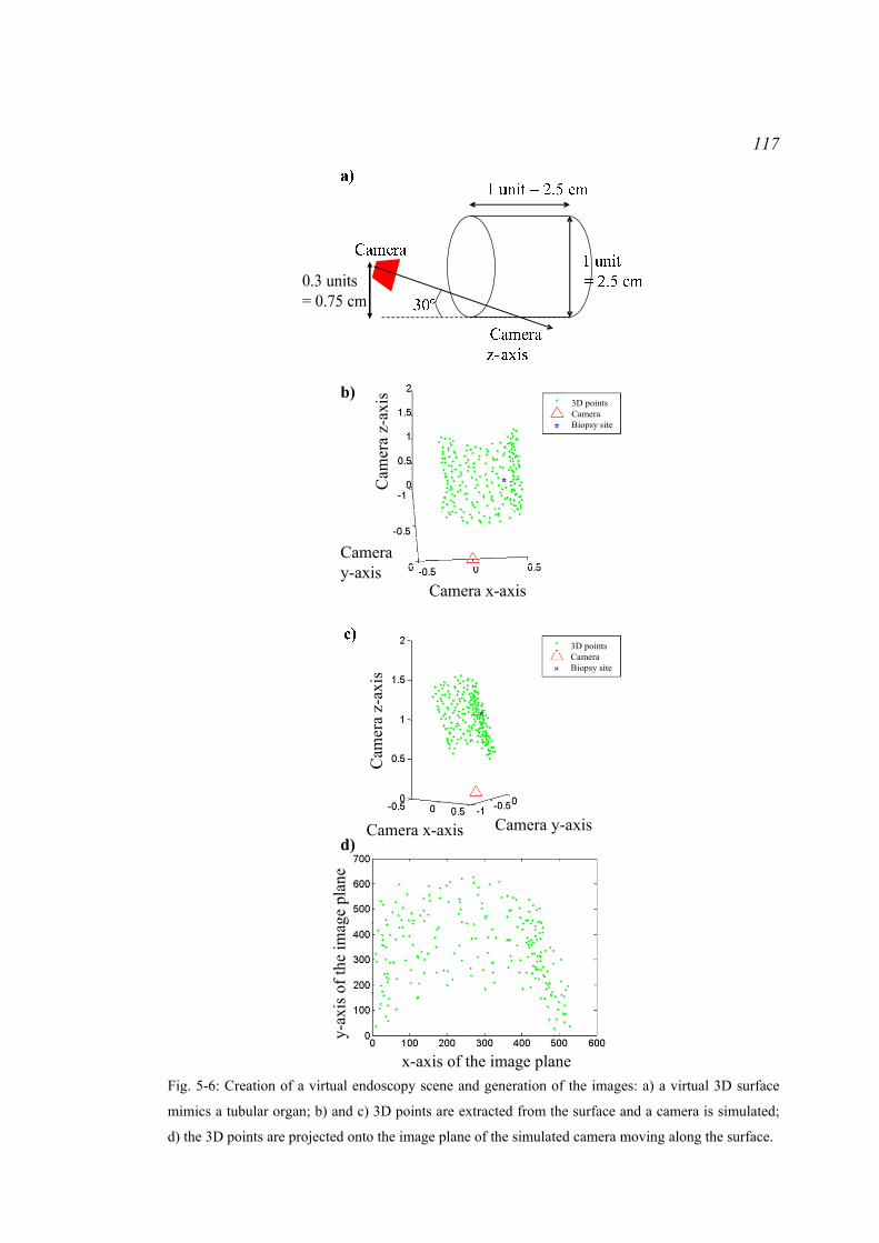
117
0.3 units= 0.75 cm
b)C
amer
a z-
axis
Camera x-axis
Cameray-axis
3D pointsCameraBiopsy site
Cam
era
z-ax
is
Camera x-axis Camera y-axis
3D pointsCameraBiopsy site
d)
x-axis of the image plane
y-ax
is o
f the
imag
e pl
ane
Fig. 5-6: Creation of a virtual endoscopy scene and generation of the images: a) a virtual 3D surface
mimics a tubular organ; b) and c) 3D points are extracted from the surface and a camera is simulated;
d) the 3D points are projected onto the image plane of the simulated camera moving along the surface.

118
The virtual scene reproduced a section of a hollow organ, such as an oesophagus,
which can be described by a cylinder of diameter 2.5cm (Fig. 5-6 a)). A virtual camera
representing an endoscope camera was placed within this virtual scene at a distance of
approximately 0.75cm from the tissue surface and had an inclination of 30° in order to
observe only an extent of the cylinder. The inclination was set at 30° since this was the angle
that could be assumed from the endoscopic images acquired on real patients. Moreover, the
camera was placed at a distance of 0.75cm from the surface since sequences extracted from
real endoscopy examinations showed that the camera is commonly at this distance using the
miniprobe as a scale within the image.
Three-D points were extracted at regular distances from this cylinder in order to
represent the features of the oesophagus and perturbed with an isotropic Gaussian noise in the
x, y, and z directions in order to obtain an irregular distribution of points in the 3D space
(Fig. 5-6 b) and c)). During an optical biopsy and a biopsy excision with forceps in real
endoscopic sequences in Barrett’s Oesophagus (BO), the camera usually observes a small
region of the oesophagus which can be its bottom half, for example. Features detected in this
region correspond to tissue points on an extent of 2cm x 2cm according to real endoscopic
images. Thus, only half of the 3D points were used for the simulations, and the 3D-points
were extracted only along a 2.5cm height of the cylinder. In Chapter 4 section ‘4.3.2
Experiment: number of matches for the computation of the fundamental matrix’, it was
mentioned that approximately 100 feature matches would be used for the recovery of the
epipolar geometries in real endoscopic images of 300 pixels x 300 pixels. In these
simulations, 200 3D points were created such that various samples of 100 features could be
used for the recovery of the epipolar geometries.
The camera was translated and rotated within this scene in a neighbourhood of a
1.5cm diameter centred on the initial camera position. During real endoscopy examinations of
the oesophagus, it was possible to twist the endoscope up to 45° which is why the camera was
rotated up to this angle. For each camera pose, the 3D points were projected onto the image
plane Ii of the camera (Fig. 5-6 d)).
A 3D point was selected randomly among the 200 3D points to be the biopsy site
(Fig. 5-6 b) and c)). This point had, therefore, a known location ( )iIp in the reference images
Ii. The last image was considered as the target image T where the biopsy site needed to be re-
localised. The ground-truth position of this site was defined as p0.
For each pair of images Ii ↔ T, α% of the features in the target image T were
displaced anywhere within its field of view to create outliers. A Gaussian noise of standard
deviation varying from 0.1 pixel to 4 pixels was added to the inliers. These figures were used

119
by Hartley (1997) and Csurka et al. (1997) for images or simulated images that had a field of
view of hundreds of pixels. The re-localised biopsy site was computed for each Gaussian
noise. The impact of the noise and of the outliers on the re-localised biopsy site was studied
by estimating the root mean squared error (RMS) of the re-localisation for each standard
deviation of the Gaussian noise. The definition of the error was inspired from West et al.
(1999) who measured the Euclidean distance between the ground-truth of a point and its
estimate. In these simulations, the error was defined as the Euclidean distance of the re-
localised biopsy site to the ground-truth p0. For each standard deviation of the Gaussian
noise, the re-localised biopsy site was computed 1000 times and the RMS error was defined
as (West et al., 1999):
( )∑=
−⋅=1000
1
2
21-10001RMS
k
k0pp .
(5-8)
where p(k) is the kth estimate of the biopsy site. By development:
( )
( ) 2
2mean
1000
1
2
2mean
1000
1
2
2
2
1-10001000
1-10001
1-10001RMS
0
0
pppp
pp
−⋅+−⋅=
−⋅=
∑
∑
=
=
k
k
k
k
.
(5-9)
The first term of the sum is the experimental precision:
( )∑=
−⋅=1000
1
2
2mean1-10001precision
k
k pp . (5-10)
where pmean = [xmean, ymean] tr is the mean of the biopsy sites p(k). The second term is the bias:
2
2mean2
1-10001000 bias 0pp −⋅= .
(5-11)
The generation of a virtual 3D scene and the corresponding analysis were repeated
twice:
- the first study was performed with 30% outliers among the matches which corresponds to
the proportion counted manually in the last experiment in Chapter 4 section ‘4.3.2
Experiment: number of matches for the computation of the fundamental matrix’. The re-
localised biopsy site was computed with 2 epipolar lines, first, and with 50 epipolar lines,
secondly. The number 50 was chosen since for some real endoscopic sequences a similar
order of images was used for biopsy site re-localisation.
- the second study was performed with 20% outliers among the matches. The re-localised
biopsy site was computed with 2 epipolar lines, first, and with 10 epipolar lines, secondly,
since for other real endoscopic sequences approximately 5 to 15 images were used for the
biopsy site re-localisation.

120
The images generated from the projections of the 3D surface onto the camera image
plane for each viewpoint were free of noise and outliers. For this experiment, each pair of
images Ii ↔ T was modified as follows:
1. 100 matches were selected randomly among the 200 matches since this number
corresponds approximately to that used for the estimation of the epipolar geometry
on patient data.
2. For 1000 repeats:
a. In image T select randomly α% of the matches and move them by a random
displacement within the image in order to create outliers. Indeed, a feature in
T forms an outlier with a feature in Ii if the two features do not correspond to
the same point at the surface of the object.
b. Apply a Gaussian noise sample of standard deviation σ to the features in T.
The experiments in section ‘4.2.2 Experiment: study of the error for the
localisation of the features’ demonstrated that these are strong assumptions.
Nevertheless, these simulations just aimed to generate uncertainty of the
epipolar lines in order to study the variations of the location of the re-
localised biopsy site p. Thus, the noise could be modelled freely.
c. Apply a noise sample of standard deviation σ to the features in the images Ii.
The biopsy site ( )iIp was perturbed by the noise as well.
d. Recover the epipolar geometry formed by the pair of images Ii ↔ T. Derive
the epipolar lines in T from the biopsy site ( )iIp in Ii.
Thus, for each pair of images Ii ↔ T, there were 1000 estimations of the epipolar
line. Steps 1. and 2. were repeated for a standard deviation of the Gaussian noise σ varying
from 0.1 pixels to 4 pixels.
3. For each value σ of the standard deviation of the noise:
a. For each repeat, re-localise the biopsy site either with 2 epipolar lines or with
N epipolar lines. Two sets of 1000 re-localised biopsy sites p(k) = [px(k), py
(k)] tr
in the target image T were computed: there was one set for the re-localisation
with 2 epipolar lines and one set for the re-localisation with N epipolar lines.
b. For each set of re-localised biopsy sites, the experimental precision and bias
of the re-localisation method were computed (equations (5-10) and (5-11)).
The re-localised biopsy site p was estimated 1000 times. It was assumed that the re-
localised biopsy sites computed with N epipolar lines were close to the true location of p and
there was no need to detect outliers for the computation of the precision and of the bias.
However, the re-localisation with 2 epipolar lines could return biopsy sites that were very far

121
from p. Indeed, p can be anywhere within the overlap of the two envelopes of the epipolar
lines (Fig. 5-7). The true location of the biopsy site or ground truth was located where the
arms of the hyperbolas narrow to a minimum. The simulations aimed to study the variations
of the precision and bias of the re-localised biopsy site with the noise on the matches.
Therefore, only the re-localised biopsy sites located around the ground truth were used for
this study. Fifty percent of these sites were used as inliers and it was assumed that their
distribution around the ground truth was Gaussian. These inliers were detected by the
minimum volume ellipsoid algorithm (Rousseeuw and Leroy, 1987). This algorithm is as
follows:
Draw a subsample of 3 different re-localised biopsy sites p(k):
1. Compute the mean ps_mean of these 3 sites and their covariance matrix Cs_mean.
2. Compute the median m2 of the Mahalanobis distances of each re-localised biopsy site
with Cs_mean: ( ) ( ) tr)(1_
)(2meanmeansmean ppCpp −⋅⋅−= − kkmedm .
3. The volume of the resulting ellipsoid is proportional to (det(m2C))1/2.
The subsample drawing is repeated. The mean and the covariance of the distribution of the
re-localised biopsy sites correspond to those that return the minimum volume over the
drawings.
Envelop
e 2Envelope 1
Envelop
e 2
Env
elop
e 1
a) b) Fig. 5-7: Intersection of two epipolar lines and locus of the possible re-localised biopsy sites: the
epipolar lines are characterised by their envelope whose thickness represents the confidence level
(50% confidence, for example). The lines can be anywhere within this envelope with the
corresponding probability. The re-localised biopsy site is in the region corresponding to the overlap of
the two envelopes. The overlap depends on the angle that the two epipolar lines subtend: a) the two
epipolar lines subtend a large angle; b) the two epipolar lines subtend a small angle.

122
5.3.2 Results
The matches between the images Ii and the target image T were contaminated with a
Gaussian noise and a certain percentage of matches was displaced in order to create outliers.
When the standard deviation of the noise increases, the features may lie far from their true
location. The resulting feature matches can be outliers for the epipolar geometry. Thus, the
epipolar geometry is recovered from less inliers. Luong and Faugeras (1996), Hartley and
Zisserman (2004), and Hu et al. (2008b) showed that the epipolar geometry and, therefore,
the epipolar lines are recovered with less precision when less inliers are used. Therefore, the
epipolar lines may be further away from the location of the ground-truth and their orientation
angle determined by the envelope is larger (Csurka, 1997; Hartley and Zisserman, 2004). In
order to illustrate this property of inaccuracy, an example of the behaviour of an epipolar line
( ) ( ) ( ) ( )[ ] tr,, iiii
myx elelel IIIIel = derived from the biopsy site ( )iIp for a pair of images Ii and T with
the increasing standard deviation of the Gaussian noise is shown in Fig. 5-8. As the epipolar
geometry from which this epipolar line was derived was estimated 1000 times for each
standard deviation of the noise, the distance of this epipolar line from the ground-truth was
computed 1000 times. The accuracy of the line was defined as the root mean squared error of
the perpendicular distance of each estimation of this line to the ground-truth p0 = [x0, y0, 1] tr
(West et al., 1999):
( )
( )( ) ( )( ) ( )( )
( )( ) ( )( )∑= ⎟⎟
⎟
⎠
⎞
⎜⎜⎜
⎝
⎛
+
+⋅+⋅=
1000
1
2
22
00
10001accuracy
kk
yk
x
km
ky
kx
ii
iii
i
elel
elyelxelII
III
el I . (5-12)
In practice, it could happen that some estimates of the epipolar line out of the 1000 estimates
were wrong. These were detected using the LMedS where the error was the distance of the
estimate of the epipolar line to the ground truth of the biopsy site. When the standard
deviation of the Gaussian noise increased, the values of the accuracy of the epipolar line
increased (Fig. 5-8).
The biopsy site p is re-localised in the target image T either as the intersection of two
epipolar lines or by minimisation of a cost function C which is the sum of the perpendicular
distances from p to the epipolar lines (equation (5-7)).
For a re-localisation of the biopsy site with 2 epipolar lines, as the lines could be
further away from the ground-truth when the noise increased, their intersection could lie
further away from the ground-truth (Fig. 5-9 a)). Fifty percent of these re-localised biopsy
sites were used for the estimation of the precision (Fig. 5-9 b)). The disparity of the re-
localised biopsy sites was greater when the noise increased. Thus, for the simulations, when
the standard deviation of the Gaussian noise on the features increased, the re-localised biopsy

123
sites formed a larger point cloud around the ground truth and the value of the re-localisation
precision was higher. As the point cloud was larger, the mean of the re-localised biopsy sites
might be further away from the ground-truth p0 and the re-localisation bias might be higher
(Fig. 5-10 and Fig. 5-11).
For a re-localisation with N > 2 epipolar lines, the biopsy sites were close to the
ground-truth p0 (Fig. 5-9 c)). The value of the minimum Cmin of the cost function defined in
equation (5-7) increased as the epipolar lines were further away from the ground-truth (Fig.
5-12). As the biopsy site was estimated 1000 times, 1000 costs Cmin were determined and an
average of the costs could be computed. This cost tended to increase with an increasing noise.
Therefore, the re-localised biopsy sites were computed with less precision (Fig. 5-13 and Fig.
5-14). Their bias increased as well. For comparison, the re-localised biopsy site was also
computed by minimisation of the algebraic distance (equation (5-2)). The resulting biopsy
site was less precise than that obtained by minimisation of the perpendicular distances. The
biases were similar. Finally, precisions and biases had smaller values for re-localisation with
N > 2 epipolar lines.
This experiment consisted of adding noise and outliers among the feature matches in
order to create uncertainty of the epipolar lines. The location of the re-localised biopsy site
was less precise and more biased when the noise increased and when the epipolar lines were
less accurate. The resulting re-localised biopsy sites were less biased and more precise when
they were estimated from N > 2 epipolar lines than when they were estimated from 2 epipolar
lines.
98765432
1
0 0.5 1 1.5 2 2.5 3 3.5 4 0 0.5 1 1.5 2 2.5 3 3.5 4
7
6
5
4
3
2
1
Acc
urac
y of
an
epip
olar
line
(in p
ixel
s)
Standard deviation of the Gaussian noise on the features (in pixels)
(a)
Acc
urac
y of
an
epip
olar
line
(in p
ixel
s)
Standard deviation of the Gaussian noise on the features (in pixels)
(b) Fig. 5-8: Accuracy of an epipolar line in the target image T derived from the biopsy site in the
reference image Ii with a varying standard deviation of the Gaussian noise (a) for 30% outliers among
the feature matches and (b) for 20% outliers among the feature matches. The image dimensions were
700 pixels x 700 pixels.
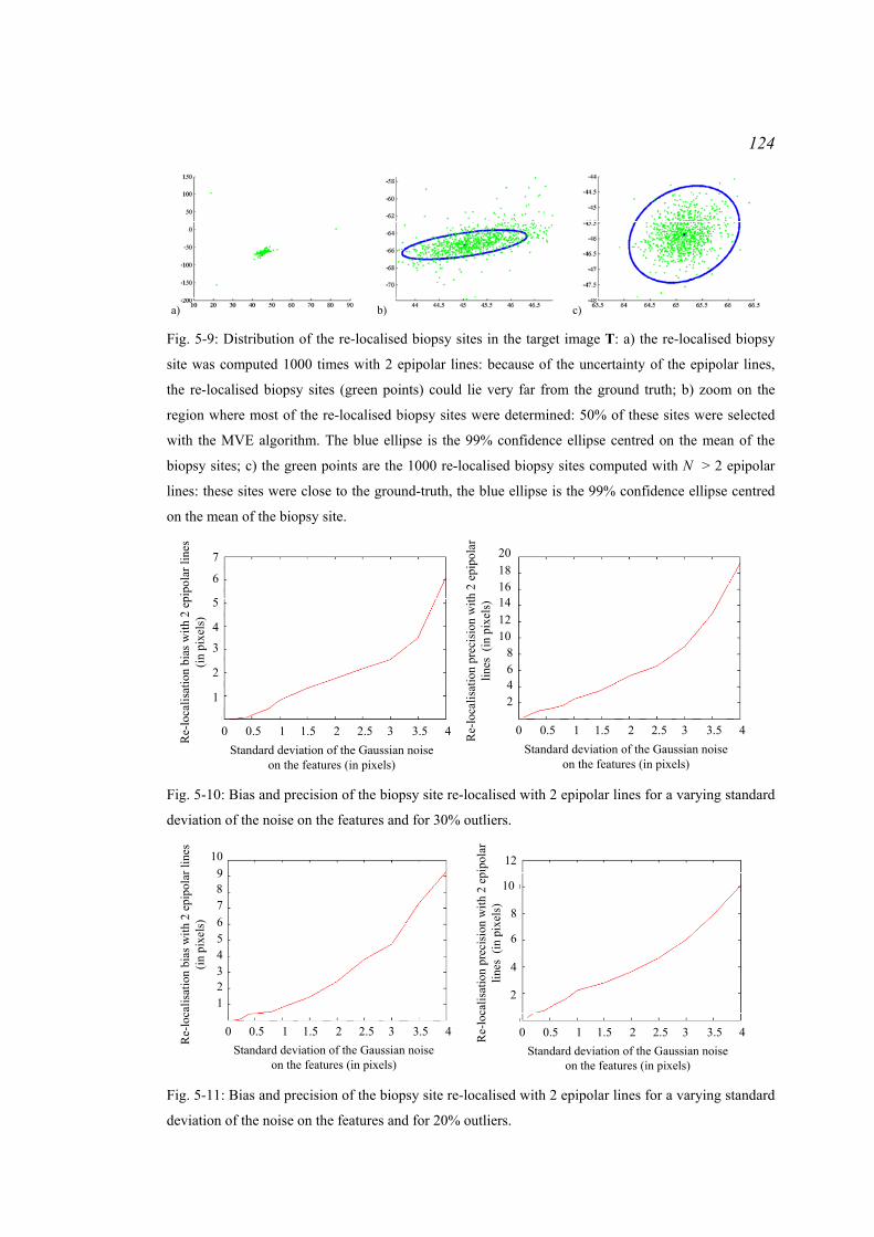
124
a) b) c) Fig. 5-9: Distribution of the re-localised biopsy sites in the target image T: a) the re-localised biopsy
site was computed 1000 times with 2 epipolar lines: because of the uncertainty of the epipolar lines,
the re-localised biopsy sites (green points) could lie very far from the ground truth; b) zoom on the
region where most of the re-localised biopsy sites were determined: 50% of these sites were selected
with the MVE algorithm. The blue ellipse is the 99% confidence ellipse centred on the mean of the
biopsy sites; c) the green points are the 1000 re-localised biopsy sites computed with N > 2 epipolar
lines: these sites were close to the ground-truth, the blue ellipse is the 99% confidence ellipse centred
on the mean of the biopsy site. R
e-lo
calis
atio
n pr
ecis
ion
with
2
epip
olar
lines
(in
pix
els)
0 0.5 1 1.5 2 2.5 3 3.5 4
7
6
5
4
3
2
1
Re-
loca
lisat
ion
bias
with
2 e
pipo
larl
ines
(in
pix
els)
Standard deviation of the Gaussian noise on the features (in pixels)
0 0.5 1 1.5 2 2.5 3 3.5 4
1816
108642
Re-
loca
lisat
ion
prec
isio
n w
ith 2
epi
pola
rlin
es (
in p
ixel
s)
Standard deviation of the Gaussian noise on the features (in pixels)
1214
20
Fig. 5-10: Bias and precision of the biopsy site re-localised with 2 epipolar lines for a varying standard
deviation of the noise on the features and for 30% outliers.
0 0.5 1 1.5 2 2.5 3 3.5 4
10
8
6
4
2
Standard deviation of the Gaussian noise on the features (in pixels)
Re-
loca
lisat
ion
prec
isio
n w
ith 2
ep
ipol
arlin
es (
in p
ixel
s)
0 0.5 1 1.5 2 2.5 3 3.5 4
98
54321
Re-
loca
lisat
ion
prec
isio
n w
ith 2
epi
pola
rlin
es (
in p
ixel
s)
Standard deviation of the Gaussian noise on the features (in pixels)
67
10 12
Re-
loca
lisat
ion
bias
with
2 e
pipo
larl
ines
(in
pix
els)
Fig. 5-11: Bias and precision of the biopsy site re-localised with 2 epipolar lines for a varying standard
deviation of the noise on the features and for 20% outliers.

125
0.5 1 0.5 2 2.5 3 3.5 4Standard deviation of the Gaussian noise on
the features (in pixels)
0
500
1000
1500
2000
2500
3000
3500
4000A
vera
ge o
f Cm
in(in
pix
els2 )
0.5 1 1.5 2 2.5 3 3.5 4Standard deviation of the Gaussian noise on
the features (in pixels)
00
50
100
150
200
250
300
350
Ave
rage
of C
min
(in p
ixel
s2 )
(a) Percentage of outliers α = 30%, Number of epipolar lines N = 50
(b) Percentage of outliers α = 20%, Number of epipolar lines N = 10
0
Fig. 5-12: Average of the minimum Cmin of the cost function C used for the computation of the re-
localised biopsy site with N epipolar lines for a varying standard deviation of the noise on the features.
R
e-lo
calis
atio
n pr
ecis
ion
with
2
epip
olar
lines
(in
pix
els)
0 0.5 1 1.5 2 2.5 3 3.5 4
1.41.2
10.80.60.40.2
Re-
loca
lisat
ion
bias
with
Nep
ipol
arlin
es (
in p
ixel
s)
Standard deviation of the Gaussian noise on the features (in pixels)
0 0.5 1 1.5 2 2.5 3 3.5 4
6
3
2
1
Re-
loca
lisat
ion
prec
isio
n w
ith N
epip
olar
lines
(in
pix
els)
Standard deviation of the Gaussian noise on the features (in pixels)
4
5
7
1.61.8
2Perpendicular distanceAlgebraic distance
Perpendicular distanceAlgebraic distance
Fig. 5-13: Bias and precision of the biopsy site re-localised with 50 epipolar lines for a varying
standard deviation of the noise on the features and for 30% outliers.
Re-
loca
lisat
ion
prec
isio
n w
ith 2
ep
ipol
arlin
es (
in p
ixel
s)
0 0.5 1 1.5 2 2.5 3 3.5 4
1
0.5
Re-
loca
lisat
ion
bias
with
Nep
ipol
arlin
es (
in p
ixel
s)
Standard deviation of the Gaussian noise on the features (in pixels)
0 0.5 1 1.5 2 2.5 3 3.5 4
6
3
2
1
Re-
loca
lisat
ion
prec
isio
n w
ith N
epip
olar
lines
(in
pix
els)
Standard deviation of the Gaussian noise on the features (in pixels)
4
5
71.5Perpendicular distanceAlgebraic distance
Perpendicular distanceAlgebraic distance
Fig. 5-14: Bias and precision of the biopsy site re-localised with 10 epipolar lines for a varying
standard deviation of the noise on the features and for 20% outliers.

126
5.4 Experiment 2: Study of the influence of the angle of the epipolar
lines on the accuracy of the re-localised biopsy site using patient data
The biopsy site may be re-localised from a set of N ≥ 2 epipolar lines. As the lines are
computed with uncertainty, they vary in direction and accuracy within an envelope which is a
hyperbola. Therefore, the epipolar lines are likely to pass a few pixels away from the biopsy
site in the target image T. Furthermore, the camera movement is limited in the oesophagus
and many epipolar lines may subtend a very small angle, especially the lines derived from
consecutive video images. These experiments aimed to study the influence of the angle
subtended by the epipolar lines on the re-localised biopsy site.
5.4.1 Materials and method
Two sequences acquired during gastroscopy were processed for a re-localisation with
respectively 2 epipolar lines and N > 2 epipolar lines.
For 2 epipolar lines, the processed sequence showed a miniprobe inserted into the
working channel of the endoscope. The miniprobe was touching the tissue for interrogation
and was removed for tissue excision. When the tissue was scanned with the miniprobe, the
endoscope camera could move up and down to generate multiple viewpoints. The biopsy site
was located at the tip of the miniprobe. A mark was located next to the biopsy site which
helped track the biopsy site location in the images where the miniprobe did not appear. The
biopsy site location was tracked manually through the images until the target image, for
convenience determined as the last image of the sequence. The epipolar geometry was
computed for each pair of reference image Ii and target image T. The epipolar lines were
derived and the biopsy site was re-localised with 2 epipolar lines derived from 2 consecutive
reference images first and subsequently from 2 different viewpoints.
For N epipolar lines, the processed sequence was acquired without the miniprobe in
the field of view. The biopsy site was identified as the mark on the tissue and a gold standard
position p0 was retrieved. As there was no miniprobe inserted, the camera movement is larger
and the viewpoints were very different. Thus, the derived epipolar lines subtended angles
larger than 90°. Twenty epipolar lines were selected to subtend an angle whose value varied
from 10° to 90°. For each angle value, the biopsy site was re-localised with the 20 selected
epipolar lines. Twenty lines were selected as this is a high number of lines for biopsy site re-
localisation in practice. This computation was repeated 100 times for each angle value and
there were 100 estimations p(k) of the re-localised biopsy site. The accuracy of the re-
localisation was estimated as the RMS error of the distances between p(k) and p0 (equation
(5-8)).
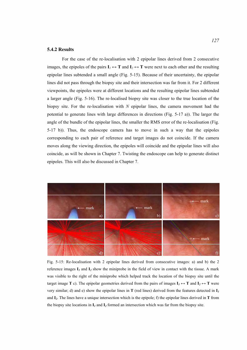
127
5.4.2 Results
For the case of the re-localisation with 2 epipolar lines derived from 2 consecutive
images, the epipoles of the pairs I1 ↔ T and I2 ↔ T were next to each other and the resulting
epipolar lines subtended a small angle (Fig. 5-15). Because of their uncertainty, the epipolar
lines did not pass through the biopsy site and their intersection was far from it. For 2 different
viewpoints, the epipoles were at different locations and the resulting epipolar lines subtended
a larger angle (Fig. 5-16). The re-localised biopsy site was closer to the true location of the
biopsy site. For the re-localisation with N epipolar lines, the camera movement had the
potential to generate lines with large differences in directions (Fig. 5-17 a)). The larger the
angle of the bundle of the epipolar lines, the smaller the RMS error of the re-localisation (Fig.
5-17 b)). Thus, the endoscope camera has to move in such a way that the epipoles
corresponding to each pair of reference and target images do not coincide. If the camera
moves along the viewing direction, the epipoles will coincide and the epipolar lines will also
coincide, as will be shown in Chapter 7. Twisting the endoscope can help to generate distinct
epipoles. This will also be discussed in Chapter 7.
a) b) c)
mark mark
mark
mark
d) e) f) Fig. 5-15: Re-localisation with 2 epipolar lines derived from consecutive images: a) and b) the 2
reference images I1 and I2 show the miniprobe in the field of view in contact with the tissue. A mark
was visible to the right of the miniprobe which helped track the location of the biopsy site until the
target image T c). The epipolar geometries derived from the pairs of images I1 ↔ T and I2 ↔ T were
very similar; d) and e) show the epipolar lines in T (red lines) derived from the features detected in I1
and I2. The lines have a unique intersection which is the epipole; f) the epipolar lines derived in T from
the biopsy site locations in I1 and I2 formed an intersection which was far from the biopsy site.
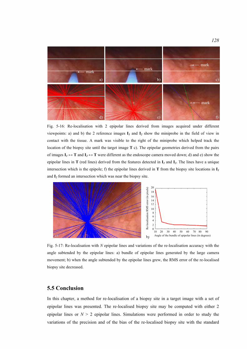
128
a) b) c)
markmark
mark
mark
d) e) f) Fig. 5-16: Re-localisation with 2 epipolar lines derived from images acquired under different
viewpoints: a) and b) the 2 reference images I1 and I2 show the miniprobe in the field of view in
contact with the tissue. A mark was visible to the right of the miniprobe which helped track the
location of the biopsy site until the target image T c). The epipolar geometries derived from the pairs
of images I1 ↔ T and I2 ↔ T were different as the endoscope camera moved down; d) and e) show the
epipolar lines in T (red lines) derived from the features detected in I1 and I2. The lines have a unique
intersection which is the epipole; f) the epipolar lines derived in T from the biopsy site locations in I1
and I2 formed an intersection which was near the biopsy site.
2018161412
1086420
10 20 30 40 50 60 70 80 90Angle of the bundle of epipolar lines (in degrees)
Re-
loca
lisat
ion
RM
S er
ror (
in p
ixel
s)
Fig. 5-17: Re-localisation with N epipolar lines and variations of the re-localisation accuracy with the
angle subtended by the epipolar lines: a) bundle of epipolar lines generated by the large camera
movement; b) when the angle subtended by the epipolar lines grew, the RMS error of the re-localised
biopsy site decreased.
5.5 Conclusion
In this chapter, a method for re-localisation of a biopsy site in a target image with a set of
epipolar lines was presented. The re-localised biopsy site may be computed with either 2
epipolar lines or N > 2 epipolar lines. Simulations were performed in order to study the
variations of the precision and of the bias of the re-localised biopsy site with the standard

129
deviation of the Gaussian noise on the features and, therefore, with a greater uncertainty of
the epipolar lines. The simulations showed that the re-localisations were more precise and
less biased when the noise on the feature matches increases. Moreover, the experiments on
patients showed that the angle formed by the epipolar lines is also important for an accurate
re-localisation and that a re-localised biopsy site computed from only 2 epipolar lines risks
being far away from the true location of the biopsy site. Thus, the re-localisation with N > 2
epipolar lines is preferred.
The re-localisation methods return the location of a point. During endoscopy
procedures, these methods could be applied for guidance of forceps to the biopsy site for
tissue excision or of optical biopsy miniprobes for a tissue interrogation. Forceps usually
extract a tissue extent of 5mm. In practice, the re-localisation methods could be extended
with the display of a confidence region around the re-localised biopsy site. The next chapter
presents a way to estimate this region for a re-localised biopsy site computed from N > 2
epipolar lines.
130
Chapter 6 Uncertainty of the Re-localised Biopsy Site
6.1 Introduction
In the previous chapter, a method was presented to re-localise a biopsy site in a target
endoscopic image. The re-localisation is based on the use of epipolar lines derived from the
biopsy site location in N reference endoscopic images. The number of lines N can be 2 or
greater. However, this re-localisation method returns a point only. An endoscopist may be
interested, instead, in a measure of the confidence with which the biopsy site was re-
localised. Such a measure can be either the precision with which the biopsy site was re-
localised or the uncertainty.
The precision measures how close independent re-localisations of the biopsy site are
(ISO 5725-1: 1994; Menditto et al., 2007). If the method is biased, the average value of a
series of independent re-localisations is deviated from the true location of the biopsy site
(Menditto, 2007). If the method is not biased or if the bias is small, the precision is an
indicator of the accuracy which measures the closeness of agreement between the re-localised
biopsy site and its true location.
The uncertainty returns a range of locations within which the true biopsy site is
asserted to lie (ISO 5725-1: 1994). Csurka et al. (1997), Zhang (1998), and Hartley and
Zisserman (2004) showed that the uncertainty of a fundamental matrix or of an epipolar line
may be characterised by its covariance matrix. This definition can be applied to the re-
localised biopsy site. Thus, when a biopsy site is re-localised, its covariance matrix is
computed as well. From this matrix, a confidence region centred on the re-localised biopsy
site can be displayed in the target image T. This region can help the endoscopist guide the
forceps to excise the tissue extent corresponding to the optical measurement done by optical
biopsy.
Csurka et al. (1997), Zhang (1998), and Hartley and Zisserman (2004) presented
experimental and analytical methods to estimate the uncertainty of the fundamental matrix
and of the epipolar lines. This chapter presents a method to compute analytically the
uncertainty and the precision of the re-localised biopsy site. The analytical derivation was
published first in Allain et al. (2010). Results of the comparison of the experimental and
analytical uncertainties using the simulations of Chapter 5 and using patient data are
discussed.
131
6.2 Experimental and analytical computations of the uncertainty of a
vector
The uncertainty or covariance matrix can be computed experimentally with a series of
estimations of the re-localised biopsy site or analytically using the implicit function theorem.
6.2.1 Confidence ellipse and precision
The derivation of the experimental and analytical uncertainty is presented using a general
random vector x = [ xx , xy ] tr∈IRm.
For the description of the uncertainty of x with the display of a confidence ellipse, it
is assumed that the random vector x follows a Gaussian distribution of mean E[x] and of
covariance matrix Λx:
( ) ( )[ ] ⎥⎦
⎤⎢⎣
⎡=−⋅−=
yyyx
yxxxEEExxxx
xxxxx xxxxΛ
varcovcovvar
][][ tr . (6-1)
Under this assumption, the quantity δx = (x – E[x])tr . Λx-1 . (x – E[x]) follows a χ2 distribution
of 2 degrees of freedom and, given a scalar k, the probability Pχ2(k , 2) that δx appears
between 0 and k is known (Csurka et al., 1997). The probability that x lies inside the ellipse
defined by the equation (x – E[x])tr . Λx-1 . (x – E[x]) = k2 where k is any scalar is equal to
Pχ2(k , 2). In order to draw the 99% confidence ellipse, for example, k has to be found such
that Pχ2(k , 2) = 0.99.
The covariance matrix can be computed experimentally or analytically.
6.2.2 Experimental estimation of the uncertainty and of the precision
Csurka et al. (1997), and Zhang (1998) showed that the covariance matrix of a vector, for
example the fundamental matrix or the epipolar line, can be estimated experimentally.
The experimental method returns M estimations xk of the vector x and approximates
the mean of the vector with the discrete mean defined as:
[ ] ∑=
=M
kkkM M
E1
1 xx . (6-2)
The covariance matrix Λx_experimental is approximated by:
[ ]( ) [ ]( )[ ]∑=
−⋅−−
=M
kkMkkMk EE
M 1
tralexperiment_ 1
1 xxxxΛx . (6-3)
A confidence region can be drawn under the assumption that x follows a Gaussian
distribution. The measure of the precision may be also useful as an indicator of the accuracy
of the estimation of the vector x. In the previous chapter, the precision was derived from the

132
root mean squared error (equation (5-10)). When applied to the vector x with the notations of
this Chapter, the precision can be defined as:
[ ]
yyxx
M
kkk E
M
xxxx
xx
varvar
11precision
1
2
2
+=
−⋅−
= ∑= .
(6-4)
There is a normalisation by M-1 in order to compute an unbiased estimator of the precision
(Johnson and Wichern, 1998).
In practice, when x refers to the re-localised biopsy site, it is estimated M times by
adding a Gaussian noise to the matches of the pair of images Ii and T for each estimation.
This noise creates variance of the epipolar lines which results in a variance of the re-localised
biopsy site. However, such a method adds noise to matches that are already noisy in real
images. Therefore, this method may overestimate the uncertainty of the re-localised biopsy
site. Furthermore, this method requires several computations of the epipolar geometries
formed between images Ii and T which is time-consuming.
An analytical derivation can help avoid the issues that the experimental estimation of
the uncertainty and of the precision cause.
6.2.3 Error propagation for the analytical estimation of the uncertainty
Csurka et al. (1997) and Zhang (1998) presented an analytical method to estimate the
uncertainty of the fundamental matrix and of the epipolar lines. This method is based on a
proposition of error propagation and on the implicit function theorem. They were presented
already in Csurka et al. (1997) and Zhang (1998) and are stated again here as they make some
important assumptions for the case of the re-localised biopsy site
Let the general random vector y = [ yx , yy ] tr ∈IRp be derived from the random vector
x = [ xx , xy ]tr ∈ IRm such that ( )xy ϕ= where φ is a C1 function. The Taylor expansion of φ
at the first order in the neighbourhood of E[ x ] returns:
( ) [ ]( ) [ ]( ) [ ]( ) ( )xxxxDxx Ο+−⋅+= EEE ϕϕϕ . (6-5)
Dφ is the Jacobian of the function φ.
Under the assumption that any sample of x is close to E[ x ], the function φ can be
approximated by its first-order term:
[ ] [ ]( )xy EE ϕ≈ . (6-6)
( ) [ ]( ) [ ]( ) [ ]( )xxxDxx EEE −⋅≈− ϕϕϕ . (6-7)
Proposition 1: The covariance matrix Λy of the vector y is therefore:

133
( ) ( )[ ]( ) ( )[ ]( ) ( ) ( )[ ]( )[ ]
[ ]( ) [ ]( ) [ ]( ) [ ]( )[ ][ ]( ) [ ]( ) [ ]( )[ ] [ ]( )[ ]( ) [ ]( ) tr
trtr
trtr
tr
tr
][][
xDΛxD
xDxxxxxD
xDxxxxxD
xxxx
yyyyΛ
x
y
EE
EEEEE
EEEEE
EEE
EEE
ϕϕ
ϕϕ
ϕϕ
ϕϕϕϕ
⋅⋅=
⋅−⋅−⋅=
⋅−⋅−⋅=
−⋅−=
−⋅−=
.
(6-8)
In some situations like the computation of the fundamental matrix or of the biopsy
site re-localised with N epipolar lines, y is determined by minimisation of a criterion function
Q over the samples of x:
( ) min,min QQ =yxy
. (6-9)
The function φ and its Jacobian Dφ are, therefore, unknown and the uncertainty of y cannot be
estimated from Proposition 1 directly. The implicit function theorem may be applied in order
to determine an estimation of Dφ (Spivak, 1979; Faugeras, 1993). The theorem states:
Implicit function theorem:
Let a criterion function Q: IRm × IRp → IR be a function of class C∞, x0 ∈ IRm be the
measurement vector and y0 ∈ IRp be a local minimum of Q(x0, y). If the Hessian H of Q with
respect to y is invertible at (x, y) = (x0, y0) then there exists an open set U’ of IRm containing
x0, an open set U” of IRp containing y0, and a C∞ mapping φ: IRm → IRp such that for (x, y) in
U’× U” there is an equivalence between the two relations ‘y0 is a local minimum of Q(x, y)
with respect to y’ and ‘y = φ(x)’, and:
( ) ( )( )
00
00
yyxx
yx00 xyxΦHyxD
==
−
∂∂
⋅−=,, 1
,ϕ . (6-10)
where Φ is the curve defined by the equation:
( ) ( ) tr,,
yyxyxΦ
∂∂
=Q
and H is the Hessian matrix of the criterion Q with respect to y:
( )( )
yyxΦH yx ∂
∂=
,,
In case x0 and y0 are sufficiently close to E[x] and to E[y], Equation (6-8) becomes:
( )( ) ( )
( )tr
,
tr1
,,, −
==
==
− ⋅∂
∂⋅⋅
∂∂⋅=
00
00
00
00 yx
yyxx
x
yyxx
yxy Hx
yxΦΛx
yxΦHΛ . (6-11)

134
Csurka et al. (1997) and Zhang (1998) demonstrated that in case the criterion function Q is a
sum of l squared criteria Qj such that ( ) ( )∑=
=l
jjjQQ
1
2 ,, yxyx with x = [x1tr , …, xj
tr ,
…, xltr] tr, Φ and H become (Press et al., 1988):
( ) ( ) ( )∑= ∂
∂⋅=
l
j
jjjj
1
tr,,2,
yyx
yxyxΦ
( )( ) ( )
∑= ∂
∂⋅
∂
∂≈
l
j
jjjj QQ
1
tr
,
,,2
yyx
yyx
H yx
and ( ) ( ) ( )
∑= ∂
∂⋅
∂
∂≈
∂∂ l
j
jjjj QQ
1
tr ,,2,
xyx
yyx
xyxΦ
.
The covariance matrix Λy of the vector y is therefore:
( )( ) ( )
( ) ( )( )
tr,
tr
1,
tr1
,
,,
,,4
−
==
==
===
==
−
⋅⎥⎥
⎦
⎤
∂
∂⋅
∂
∂
⎢⎢
⎣
⎡⋅⋅
∂
∂⋅
∂
∂⋅= ∑
00
00
00
00
00
00
yx
yyxx
yyxx
x
yyxx
yyxx
yxy
Hy
yxx
yx
Λx
yxy
yxHΛ
kkkk
jjjj
kkkk
l
kj
jjjj
(6-12)
Under the assumption that the xj’s are not correlated, cov(xj, xk) = 0 and Λx = diag(Λx1, Λx2,
…, Λxl). Equation (6-12) becomes:
( )( ) ( )
( ) ( )( )
tr,
tr
1
tr1
,
,,
,,4
−
==
==
===
==
−
⋅⎥⎥⎥
⎦
⎤
∂
∂⋅
∂
∂
⎢⎢⎢
⎣
⎡⋅⋅
∂
∂⋅
∂
∂⋅= ∑
00
0
0
0
0
00
0
000
yx
yyxx
yyxx
x
yyxx
yyxx
yxy
Hy
yxx
yx
Λx
yxy
yxHΛ
jjjj
jjjj
jj
j
jj
l
jj
j
jjjj
.
(6-13)
According to equation (6-8), the first order approximation of ΛQj in the neighbourhood of the
point (xj0 , y0) is:
( ) ( ) tr,,
0
0
0
0yy
xxx
yyxx x
yxΛ
xyx
Λ==
== ∂
∂⋅⋅
∂∂
=jjjj j
jjj
j
jjQj
QQ .
(6-14)
Equation (6-13) becomes:
( )( ) ( )
( )tr
,1
tr1
,
,,4 −
===
==
− ⋅∂
∂⋅⋅
∂∂
⋅= ∑ 00
0
0
0
000 yx
yyxx
yyxx
yxy Hy
yxΛ
yyx
HΛl
j
jjQj
jj
jjjj
QQ.
(6-15)

135
Finally, under the assumption that Qj has a zero mean and that the Qj’s are independent and
have identical distributed errors (Anderson, 1958):
( )pl
QQpl
l
jjjQQj −
=−
== ∑=
min
1
200 ,1 yxΛΛ .
(6-16)
where p is the number of parameters or the dimension of y. Thus, the covariance matrix Λy of
y can be approximated by:
( ) ( ) ( ) ( )tr
,mintr
,,1
,min 22 −−−
−=⋅⋅
−=
00000000 yxyxyxyxy HHHHΛpl
Qpl
Q.
(6-17)
The proposition for error propagation and the implicit function theorem have been
applied by Csurka et al. (1997) and Zhang (1998) for the analytical computation of the
uncertainty of the fundamental matrix and of the epipolar lines. In this thesis, these
proposition and theorem are applied for the computation of the uncertainty of the re-localised
biopsy site.
6.3 Derivation of the uncertainty of the re-localised biopsy site
The experimental and analytical derivations can be adapted to the biopsy site re-localised
with N epipolar lines.
6.3.1 Discussion of the hypotheses of the experimental and analytical derivation
of the uncertainty in the case of the re-localised biopsy site computed with N
epipolar lines
Three assumptions have to be discussed before applying the derivations of the uncertainty to
the re-localised biopsy site. These derivations make the assumptions that the re-localised
biopsy site is determined with an error that follows a Gaussian distribution, that the epipolar
lines used for the re-localisation are uncorrelated, and that the residuals of the criterion
function to minimise in order to determine the re-localised biopsy site have zero mean and are
independent and identically distributed.
The fundamental matrix ( )TIF ,i for the pair of images (Ii, T) is determined by
minimisation of a criterion (equation (3-27)) over the Sampson’s residuals (equation (3-19))
for each pair of the L feature matches ( ( )ijIp , pj). Let Pi be defined as the vector:
( ) ( ) ( )[ ] trtrtrtrtrtr1
tr1 LLjj
iii ppppppP IIIi LL= . (6-18)
Under the assumption that the feature locations are determined sufficiently close to their
mean which are considered as the true locations of the features, the implicit function theorem
136
states that there exists a function φ which links ( )TIF ,i to the set of matches and (Csurka et al.,
1997; Zhang, 1998):
( ) ( )iTI PF ϕ=,i. (6-19)
The function φ can be approximated by its first order Taylor development in the
neighbourhood of the mean of Pi and:
( ) ( ) [ ]( ) [ ]( ) [ ]( ) ( )iiiiiiTI PPPPDPPF Ο+−⋅+== EEEi ϕϕϕ, . (6-20)
If Pi is sufficiently close to E[Pi], ( )TIF ,i is close to E[ ( )TIF ,i
]. An experiment in chapter 4
section ‘4.2.2 Experiment: study of the error for the localisation of the features’ illustrated
that the features are localised with an error that can be approximated as Gaussian. As the
feature locations and ( )TIF ,i may be related with a linear function according to equation (6-20),
the error with which ( )TIF ,i is determined is Gaussian. Csurka et al. (1997) and Zhang (1998)
made this assumption for the determination of the uncertainty of the fundamental matrix.
The epipolar lines ( )iIel = ( )TIF ,i. ( )iIp used for the biopsy site re-localisation are
derived from the fundamental matrix ( )TIF ,i and from a biopsy site location ( )iIp in image Ii.
In this derivation, the uncertainty of ( )iIp is not taken into account since the re-localised
biopsy site is computed from the epipolar line ( )iIel assuming that it is derived from the true
location of the biopsy site in Ii. Thus, there is a linear relation between ( )iIel and ( )TIF ,i and
the error of the re-localisation of the epipolar line is Gaussian.
The re-localised biopsy site p in image T is computed by minimisation of a criterion
(equation (5-7)) which is based on the perpendicular distances from p to the epipolar lines:
( ) ( ) ( )[ ] trtrtrtr1 Ni III elelelel LL= . (6-21)
The implicit function theorem is applied again to find a function which links the re-localised
biopsy site to the epipolar lines. Under the first order Taylor expansion of this function, the
re-localised biopsy site is linked to the epipolar lines linearly and the error associated to its
localisation is Gaussian.
The analytical derivation of the uncertainty of the re-localised biopsy site makes the
assumption that the errors of the localisations of the epipolar lines are uncorrelated. The
epipolar lines are derived from fundamental matrices ( )TIF ,i which are themselves derived
from sets of matches ( ( )ijIp , pj) for each pair of images Ii ↔ T. When the features are detected
and tracked with the Lucas-Kanade (LK) tracker, the LK tracker is launched for each image
Ii. Therefore, the epipolar geometries for the pairs of images Ii ↔ T and Ii+1 ↔ T are derived
137
from different feature matches and the epipolar lines derived from each epipolar geometry for
the biopsy site re-localisation are independent. Thus, they are uncorrelated for the case of the
LK tracker. When Scale Invariant Feature Transform (SIFT) features are detected and
matched, features are detected once in image T and matched to the features in each image Ii.
Therefore, the fundamental matrices are derived from common features in T and the
assumption of uncorrelated epipolar lines is not satisfied. The analytical derivation cannot be
applied to the case of SIFT features.
Finally, the residuals Ci used for the computation of the re-localised biopsy site p are
defined as the perpendicular distances from p to the epipolar lines. The fundamental matrices
( )TIF ,i are computed such that the residuals follow a Gaussian distribution (Chapter 3 section
‘3.5.3.3.1 Fitting errors or residuals’). As the pair of biopsy sites ( )iIp ↔ p is an inlier, the
corresponding residual follows a Gaussian distribution as well. Also, these residuals are
divided by their standard deviation (Chapter 5 ‘5.2.3 Extension of the re-localisation with N
epipolar lines’). Therefore, these residuals are identically distributed. As the epipolar lines
derived from pairs of features detected with the LK tracker are independent, the residuals are
independent. The condition of independence will be accepted for the analytical derivation of
the uncertainty for the case of features detected and matched using the LK tracker.
The analytical derivation of the uncertainty of the re-localised biopsy site has the
advantage of avoiding a high number of repeats that the experimental derivation requires.
However, it makes many approximations.
6.3.2 Analytical estimation of the uncertainty of the biopsy site re-localised with
N > 2 epipolar lines
The analytical derivation of the uncertainty of the re-localised biopsy site presented in the
previous sections is possible only for the re-localisations with more than 2 epipolar lines.
The re-localised biopsy site is found by minimising a criterion C over the set of
epipolar lines el = [ ( )1Iel tr, …, ( )iIel tr, …, ( )NIel tr] tr since the epipolar lines do not have a
common intersection:
( ) ( )( )
( )( )( ) ( )
( )( )( )
( ) ( )
2
122
tr
2
12
2,2
1,
,tr
min
min,min
∑
∑
=
=
⎟⎟⎟
⎠
⎞
⎜⎜⎜
⎝
⎛
+
⋅=
⎟⎟⎟
⎠
⎞
⎜⎜⎜
⎝
⎛
⋅+⋅
⋅⋅=
N
i yx
N
i
ii
i
i
i
i
i
i
i
elel
C
II
I
y
ITI
ITI
ITI
yy
ely
pFpF
pFyyel
.
(6-22)
138
( ) min1
2min ,min CCCN
ii == ∑
=yy
yel .
In order to determine the covariance matrix Λp as a function of the epipolar lines, the implicit
function theorem is applied to the set of lines el and to the curve Φ(el , y) defined by the
equation:
( ) ( ) 0,,tr
=∂
∂=
yyelyelΦ C
. (6-23)
Under the assumptions that the epipolar lines are not correlated, and that the Ci’s are
independent, have identical distributed errors, and have a zero mean, it results from equation
(6-17) that:
( )
( )
( )( )( )
( )( )( )
( )( )( )
( )
( ) ( )
( )
( ) ( ) ⎥⎥
⎦
⎤
⎢⎢
⎣
⎡
++=
∂∂
∂∂⋅
∂∂
⋅≈
−⋅
=
∑=
==
2222
1
tr
,
tr-,
min
, and
,,with
2
ii
i
ii
i
i
i
i
i
i
i
yx
y
yx
xi
N
i
ii
elel
el
elel
elC
CC
pNC
II
I
II
I
pel
I
pyel
I
pyel
I
pel
pelp
I
II
yyel
yyel
yyel
2H
HΛ
.
(6-24)
The uncertainty Λp can be represented as a 99% ellipse. It is drawn from the 2
eigenvalues of Λp. If their values are small, the ellipse is small. The uncertainty Λp depends
on the term Cmin which is the sum of the perpendicular distances from the re-localised biopsy
site p to the epipolar lines ( )iIel . If the epipolar lines have been derived accurately, the term
Cmin is small and contributes to make the ellipse small. Furthermore, the uncertainty Λp
depends on the inverse of the Hessian matrix H. This matrix gives the amplitude of the
curvatures of the criterion function C around the re-localised biopsy site p. If the epipolar
lines used for the re-localisation subtend a large angle, the curvatures of C are large, the 2
eigenvalues of H are large, the 2 eigenvalues of Λp are small, and the uncertainty of the re-
localised biopsy site is small. The ellipse is, therefore, small.
The uncertainty of p depends on the accuracy of the epipolar lines and on the angles
they subtend.
6.4 Experiment: comparison of the uncertainties derived analytically
and statistically by simulations
The uncertainty of the re-localised biopsy site can be estimated either analytically or
experimentally. These 2 estimations are compared in this part.
139
6.4.1 Method
The derivation of the uncertainty Λp of the re-localised biopsy site p is based on the
assumption that p follows a Gaussian distribution N(E[p], Λp). Therefore, this validation
consisted of comparing two Gaussian distributions: one whose covariance matrix has been
derived analytically and another whose covariance matrix has been derived experimentally.
As the derivation of the analytical uncertainty is based on a lot of approximations, the
experimental uncertainty was considered as the gold standard.
The uncertainties were compared by simulations and by tests on patient data. The
simulations were similar to those conducted in Chapter 5 section ‘5.3 Experiment 1: study by
simulations of the re-localisation precision and bias with the locations of the matches
perturbed by a Gaussian noise and with the presence of outliers’. A virtual endoscopy scene
was generated and images showing the features were obtained by moving a virtual camera
within the scene. The images in these experiments were only made up of features that were
not corrupted by noise. A Gaussian noise was added to the features with a standard deviation
varying from 0.1 pixels to 4 pixels. For each standard deviation of the noise, the biopsy site
was re-localised. This procedure was repeated 1000 times. Thus, 1000 re-localised biopsy
sites p(k) were computed for each standard deviation of the noise. For the comparison of the
uncertainties, the re-localised biopsy site and its analytical uncertainty Λp_analytical were
computed a first time for each standard deviation of the Gaussian noise. It was supposed that
p was sufficiently close to E[p] considered as the true biopsy site. Afterwards, as the biopsy
site was re-localised 1000 times, the uncertainty Λp_experimental was estimated experimentally.
The mean of the re-localised biopsy site E[p] was estimated as the arithmetic mean pmean of
all of the re-localised biopsy sites pj. For each standard deviation of the Gaussian noise, the
analytical distribution Nanalytical(p, Λp_analytical) was, therefore, compared to the experimental
distribution Nexperimental(pmean, Λp_experimental). The experiment consisted of comparing first the
analytical precision precisionanalytical to the experimental precision precisionexperimental computed
as in equation (6-4). As the precision takes only into account the diagonal terms of the
uncertainty, the distributions Nanalytical and Nexperimental were also compared by measuring the
Kullback-Leibler divergence between the two distributions (Kullback, 1959).
The Kullback-Leibler (KL) divergence is a measure of the difference between the 2
probability distributions pexperimental = Nexperimental(pmean, Λp_experimental) and panalytical = Nanalytical(p,
Λp_analytical). The measure DKL1 is defined as:
( ) ( ) ( )( )∑
∈
=Xx analytical
alexperimentalexperimentanalyticalalexperimentKL xp
xpxpppD ln||1 .
(6-25)

140
The variable x is a sample of the distribution Nexperimental(pmean, Λp_experimental). DKL1 is always
positive. It is equal to zero if and only if pexperimental and panalytical agree everywhere (Cardoso,
1997; Eguchi and Copas, 2006). The divergence DKL2 to compare panalytical to pexperimental was
also measured:
( ) ( ) ( )( )∑
∈
=Xx alexperiment
analyticalanalyticalalexperimentanalyticalKL xp
xpxpppD ln||2 .
(6-26)
According to the definition of the Kullback-Leibler divergences, the two distributions
Nexperimental(pmean, Λp_experimental) and Nanalytical(p, Λp_analytical) are similar if DKL1 and DKL2 are
small and are of the same order.
For the patient data, the re-localised biopsy site and its analytical uncertainty were
estimated, first, for 3 endoscopic sequences acquired on two patients during a surveillance
examination of Barrett’s Oesophagus (BO). The image dimensions for the first patient were
339 pixels x 216 pixels. For the second patient, they were 376 pixels x 280 pixels. The last
image of the sequences was selected as the target image T. The previous images were the
reference images Ii. For the first sequence of the first patient, the biopsy site was detected at
the tip of the optical miniprobe used for an optical biopsy. The location was tracked manually
until the target image T. This returned the ground truth of the biopsy site in T. For the second
sequence of the first patient, the biopsy site was selected as a natural bulb at the surface of the
oesophagus visible in all of the images. For the sequence of the second patient, an Argon
Plasma Coagulation (APC) mark was done at the surface of the oesophagus in order to create
a ground truth of the biopsy site. Secondly, the experimental uncertainty was estimated for
comparison with the analytical uncertainty. For the estimation of the experimental
uncertainty, a Gaussian noise was added to the features of the endoscopic images. The feature
locations were already detected with a Gaussian error with the LK tracker according to
Chapter 4 section ‘4.2.2 Experiment: study of the error for the localisation of the features’.
Thus, the standard deviation of the Gaussian noise was set at 0.1 pixels in order to add a
small variation of the location of features that were already noisy. The uncertainties were
compared with the Kullback-Leibler divergences.
6.4.2 Results and discussion
6.4.2.1 Results of the simulations
The results of the comparison of the precisions and of the distributions are presented in Fig.
6-1, and Fig. 6-2, and in Table 6-1 and Table 6-2.

141
0.5 1 1.5 2 2.5 3 3.5 4
Standard deviation of the Gaussian noise on the features (in pixels)
0
1
Prec
isio
ns o
f the
re-lo
calis
ed b
iops
y si
te
(in p
ixel
s)
0.5
2
1.5
3
2.5
4
3.5
a)
0.5 1 1.5 2 2.5 3 3.5 4
Standard deviation of the Gaussian noise on the features (in pixels)
Prec
isio
ns o
f the
re-lo
calis
ed b
iops
y si
te
(in p
ixel
s)
b)
0
1
2
3
4
5
6experimental
analytical
experimental
analytical
Fig. 6-1: Comparison of the experimental and analytical precisions for various standard deviations of
the noise in the images of the simulations: the re-localised biopsy site was computed with a) 50
epipolar lines and the percentage of outliers among the matches was 30%, and with b) 10 epipolar lines
and the percentage of outliers among the matches was 20%.
The analytical and experimental precisions were of the same order and did not differ
significantly (Fig. 6-1). The variations of the experimental precision were already explained
in Chapter 5 ‘Re-localisation of Biopsy Sites during Endoscopy Examinations’. The
analytical precision depends on the value of the cost Cmin (equation (6-22)). When the noise
on the features increases, the epipolar lines are less accurate and Cmin takes greater values as
discussed in Chapter 5 ‘Re-localisation of Biopsy Sites during Endoscopy Examinations’.
Therefore, the values of the analytical precision increase. The precisions are just an indicator
of the accuracy of the re-localised biopsy site and a more advanced comparison of the
uncertainties is one that evaluates all the terms of the covariance matrices as the Kullback-
Leibler divergence does.
Divergences DKL1 and DKL2 were most of the time small of the order of 0.1 or 0.01
(Table 6-1 and Table 6-2). For cases like Table 6-1 σ = 0.6, σ = 1, σ = 1.5, σ = 2, and σ = 2.5,
and Table 6-2 σ = 1, σ = 3, and σ = 4, DKL1 and DKL2 had close and small values. For these
cases, p and pmean were close as shown in Fig. 6-2 a). The ellipses had a good overlap and
were small. This means that, in practice, the endoscopist can see that the re-localised biopsy
site p is computed accurately and that the uncertainty is small. For cases like Table 6-1 σ =
0.1, σ = 0.4, σ = 0.8, σ = 3, σ = 3.5, and σ = 4, and Table 6-2 σ = 0.1, σ = 0.6, σ = 0.8, σ = 1.5,
σ = 2.5, and σ = 3.5, DKL1 and DKL2 had small values but they differed. For these cases, p was
further from pmean as shown in Fig. 6-2 b). The ellipses did not overlap well. For cases like
Table 6-1 σ = 0.2, and Table 6-2 σ = 0.2, σ = 0.4, and σ = 2, p was at the border of the 99%
confidence ellipse drawn from the experimental uncertainty. The ellipse drawn from the
analytical uncertainty was either significantly larger or smaller than the ellipse drawn from
the experimental uncertainty as shown in Fig. 6-2 c). These results were expected since the

142
analytical derivation makes the assumption that p is close to pmean in order to approximate the
experimental uncertainty by the analytical uncertainty. An inaccurate re-localised biopsy site
p is computed from epipolar lines that are inaccurate. The term Cmin defined in equation
(6-22) becomes, therefore, larger. As the size of the ellipse drawn from the uncertainty
depends on the value of Cmin, the dimensions of the ellipse then also become larger. This
means that, in practice, the endoscopist can be provided with a quanititative visual indication
of uncertainty in the re-localisation of a target site by displaying the re-localised biopsy site p
surrounded by a large ellipse as a graphical overlay on the endoscopy image.
-24.2
-24.4
-24.6
-24.8
-25
-25.2
-25.420.4 20.6 20.8 21 21.2 21.4 21.6
y-co
ordi
nate
s of t
he im
age
(in p
ixel
s)
x-coordinates of the image (in pixels)a)
Experimental ellipse
Analytical ellipse
pmean
pGround truth
Legend:
-24.4
-24.6
-24.8
-25
-25.2
-25.4y-co
ordi
nate
s of t
he im
age
(in p
ixel
s)
b)20.4 20.6 20.8 21 21.2 21.4
x-coordinates of the image (in pixels)
-50
-55
-60
-65
-70
-75
y-co
ordi
nate
s of t
he im
age
(in p
ixel
s)
c)
30 35 40 45 50 55
x-coordinates of the image (in pixels)
Fig. 6-2: Examples of analytical and experimental 99% confidence ellipses: a) the two Kullback-
Leibler divergences were small and similar (30% outliers, σ = 0.6), b) the two divergences were small
but one was higher than the other (30% outliers, σ = 0.4), c) one of the two divergences was very high
(20% outliers, σ = 2).

143 Table 6-1: Values of DKL1, and DKL2 for re-localisations with 50 epipolar lines for varying standard
deviations of noise on the features (percentage of outliers 30%).
Standard deviation σ of the noise
0.1 0.2 0.4 0.6 0.8 1 1.5 2 2.5 3 3.5 4
DKL1 0.36 0.91 0.20 0.02 0.15 0.10 0.02 0.01 0.14 0.25 0.10 0.25
DKL2 0.01 0.28 0.02 0.01 0.04 0.03 3x10⁻³ 0.01 0.10 0.02 4x10⁻³ 0.31
Table 6-2: Values of DKL1, and DKL2 for re-localisations with 10 epipolar lines for varying standard
deviations of noise on the features (percentage of outliers 20%).
Standard deviation σ of the noise
0.1 0.2 0.4 0.6 0.8 1 1.5 2 2.5 3 3.5 4
DKL1 0.09 1.12 3.49 0.13 0.20 0.09 0.09 0.45 0.19 0.05 0.44 0.08
DKL2 0.10 0.02 0.09 0.21 0.02 0.01 0.15 1.96 0.06 0.02 0.14 0.02
6.4.2.2 Results on patients
The comparison of the experimental and analytical uncertainties was performed on patient
data. The results are presented in Fig. 6-3.
For N > 2 epipolar lines, the ellipses had similar orientations and they did not differ
much in size. The corresponding KL divergences were small and of similar orders. The
greater axis of the ellipses was smaller than 2mm (Fig. 6-3). The ellipses indicate the region
where the biopsy site is likely to lie. Because of approximations during the derivation of the
analytical uncertainties, the analytical and experimental ellipses did not overlap exactly.
Nevertheless, both ellipses define a region where the biopsy site needs to be taken. Large
ellipses in one direction indicate that the epipolar lines are too much in coincidence. If the
epipolar lines subtend sufficiently large angles, the confidence ellipses will have areas less
than 2mm which is less than half the size of the typical endoscopic biopsy forceps. In this
case, if the confidence ellipses are displayed to the operator during tissue sampling, there is a
reassurance offered that the desired tissue has indeed been sampled.
6.5 Conclusion
The display of a confidence interval around a previously marked biopsy site of interest is
extremely useful for the practicing clinician as the display of both point and regional data can
reassure that the desired sample has actually been taken in traditional forceps terms or
optically interrogated in optical biopsy terms. This confidence region is drawn from the
covariance matrix of the re-localised biopsy site that can be computed experimentally or
analytically. The analytical computation requires a single estimation of the re-localised
biopsy site and of its uncertainty. However, it makes a series of assumptions about the noise

144
on the matches and the independence of the epipolar lines. The experimental computation
does not make any assumption. However, its main disadvantage is the number of iterations
this method requires for the computation of the re-localised biopsy site and of the uncertainty.
A whole framework for biopsy site re-localisation has been proposed in Chapters 3, 4, 5, and
6. The next chapter presents the results of this method on patient data. Chapter 8 focuses on
the extension of this framework for cases where the endoscopist moves the camera too
quickly or where air/water bubbles obstruct the camera field of view.
Target image Analytical and experimental ellipses (zoom around the biopsy site)
DKL1 DKL2
0.14 0.61
0.15 1.92
0.10 0.17
2mm
2mm
2mm
Biopsy site
Biopsy site
Biopsy site
Fig. 6-3: Analytical and experimental 99% confidence ellipses for N > 2 epipolar lines in the target
image: each row corresponds to a sequence acquired on a patient and presents first the target image
with the location of the biopsy site, secondly the analytical ellipse (green) and the experimental ellipse
(blue), and finally the KL divergences.
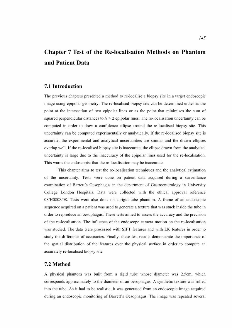
145
Chapter 7 Test of the Re-localisation Methods on Phantom
and Patient Data
7.1 Introduction
The previous chapters presented a method to re-localise a biopsy site in a target endoscopic
image using epipolar geometry. The re-localised biopsy site can be determined either as the
point at the intersection of two epipolar lines or as the point that minimises the sum of
squared perpendicular distances to N > 2 epipolar lines. The re-localisation uncertainty can be
computed in order to draw a confidence ellipse around the re-localised biopsy site. This
uncertainty can be computed experimentally or analytically. If the re-localised biopsy site is
accurate, the experimental and analytical uncertainties are similar and the drawn ellipses
overlap well. If the re-localised biopsy site is inaccurate, the ellipse drawn from the analytical
uncertainty is large due to the inaccuracy of the epipolar lines used for the re-localisation.
This warns the endoscopist that the re-localisation may be inaccurate.
This chapter aims to test the re-localisation techniques and the analytical estimation
of the uncertainty. Tests were done on patient data acquired during a surveillance
examination of Barrett’s Oesophagus in the department of Gastroenterology in University
College London Hospitals. Data were collected with the ethical approval reference
08/H0808/08. Tests were also done on a rigid tube phantom. A frame of an endoscopic
sequence acquired on a patient was used to generate a texture that was stuck inside the tube in
order to reproduce an oesophagus. These tests aimed to assess the accuracy and the precision
of the re-localisation. The influence of the endoscope camera motion on the re-localisation
was studied. The data were processed with SIFT features and with LK features in order to
study the difference of accuracies. Finally, these test results demonstrate the importance of
the spatial distribution of the features over the physical surface in order to compute an
accurately re-localised biopsy site.
7.2 Method
A physical phantom was built from a rigid tube whose diameter was 2.5cm, which
corresponds approximately to the diameter of an oesophagus. A synthetic texture was rolled
into the tube. As it had to be realistic, it was generated from an endoscopic image acquired
during an endoscopic monitoring of Barrett’s Oesophagus. The image was repeated several
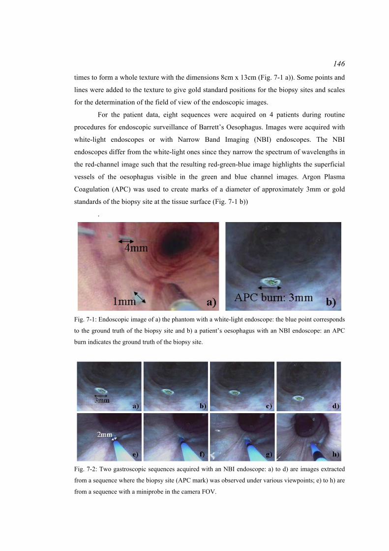
146
times to form a whole texture with the dimensions 8cm x 13cm (Fig. 7-1 a)). Some points and
lines were added to the texture to give gold standard positions for the biopsy sites and scales
for the determination of the field of view of the endoscopic images.
For the patient data, eight sequences were acquired on 4 patients during routine
procedures for endoscopic surveillance of Barrett’s Oesophagus. Images were acquired with
white-light endoscopes or with Narrow Band Imaging (NBI) endoscopes. The NBI
endoscopes differ from the white-light ones since they narrow the spectrum of wavelengths in
the red-channel image such that the resulting red-green-blue image highlights the superficial
vessels of the oesophagus visible in the green and blue channel images. Argon Plasma
Coagulation (APC) was used to create marks of a diameter of approximately 3mm or gold
standards of the biopsy site at the tissue surface (Fig. 7-1 b))
.
Fig. 7-1: Endoscopic image of a) the phantom with a white-light endoscope: the blue point corresponds
to the ground truth of the biopsy site and b) a patient’s oesophagus with an NBI endoscope: an APC
burn indicates the ground truth of the biopsy site.
Fig. 7-2: Two gastroscopic sequences acquired with an NBI endoscope: a) to d) are images extracted
from a sequence where the biopsy site (APC mark) was observed under various viewpoints; e) to h) are
from a sequence with a miniprobe in the camera FOV.
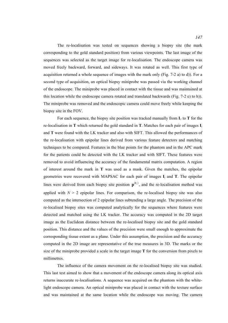
147
The re-localisation was tested on sequences showing a biopsy site (the mark
corresponding to the gold standard position) from various viewpoints. The last image of the
sequences was selected as the target image for re-localisation. The endoscope camera was
moved freely backward, forward, and sideways. It was rotated as well. This first type of
acquisition returned a whole sequence of images with the mark only (Fig. 7-2 a) to d)). For a
second type of acquisition, an optical biopsy miniprobe was passed via the working channel
of the endoscope. The miniprobe was placed in contact with the tissue and was maintained at
this location while the endoscope camera rotated and translated backwards (Fig. 7-2 e) to h)).
The miniprobe was removed and the endoscopic camera could move freely while keeping the
biopsy site in the FOV.
For each sequence, the biopsy site position was tracked manually from I1 to T for the
re-localisation in T which returned the gold standard in T. Matches for each pair of images Ii
and T were found with the LK tracker and also with SIFT. This allowed the performances of
the re-localisation with epipolar lines derived from various feature detectors and matching
techniques to be compared. Features in the blue points for the phantom and in the APC mark
for the patients could be detected with the LK tracker and with SIFT. These features were
removed to avoid influencing the accuracy of the fundamental matrix computation. A region
of interest around the mark in T was used as a mask. Given the matches, the epipolar
geometries were recovered with MAPSAC for each pair of images Ii and T. The epipolar
lines were derived from each biopsy site position ( )iIp , and the re-localisation method was
applied with N > 2 epipolar lines. For comparison, the re-localised biopsy site was also
computed as the intersection of 2 epipolar lines subtending a large angle. The precision of the
re-localised biopsy sites was computed analytically for the sequences where features were
detected and matched using the LK tracker. The accuracy was computed in the 2D target
image as the Euclidean distance between the re-localised biopsy site and the gold standard
position. This distance and the values of the precision were small enough to approximate the
corresponding tissue extent as a plane. Under this assumption, the precision and the accuracy
computed in the 2D image are representative of the true measures in 3D. The marks or the
size of the miniprobe provided a scale in the target image T for the conversion from pixels to
millimetres.
The influence of the camera movement on the re-localised biopsy site was studied.
This last test aimed to show that a movement of the endoscope camera along its optical axis
returns inaccurate re-localisations. A sequence was acquired on the phantom with the white-
light endoscope camera. An optical miniprobe was placed in contact with the texture surface
and was maintained at the same location while the endoscope was moving. The camera

148
moved along its optical axis and was such that the resulting epipolar lines should be almost
coincident. Four reference images were used to re-localise the biopsy site in the target image.
The resulting re-localised biopsy site was computed.
7.3 Results
The re-localisation results are presented in Table 7-1, Table 7-2, and Table 7-3. Biopsy sites
were re-localised in endoscopic images with an FOV of approximately 3cm x 3cm with
analytical precisions and accuracies of:
− 2.5mm or better with 2 epipolar lines after matching features with the LK tracker.
− 0.45mm or better with N > 2 epipolar lines after matching features with the LK tracker.
− 0.92mm or better with N > 2 epipolar lines after matching features with the SIFT.
The best precisions and accuracies were obtained for the sequences without a miniprobe in
the FOV.
The results presented in Table 7-1 demonstrate that a re-localisation with 2 epipolar
lines is less accurate than with N > 2 epipolar lines. The main reason is the uncertainty of the
epipolar lines. Their intersection may be, therefore, far from the true biopsy site. The use of N
> 2 epipolar lines allows the space in T, within which the re-localised biopsy site may be, to
be constrained.
Table 7-1: Results of the biopsy site re-localisation with 2 epipolar lines: for each sequence, features
were detected and matched using the LK tracker.
Sequence Miniprobe? FOV
(pixels ; cm)
Accuracy: measured distance from
the re-localised biopsy site to the gold
standard
(pixels ; mm)
Phantom Sequence 1 Yes (283 x 180 ; 3 x 4) (3.1 ; 0.20)
Phantom Sequence 2 Yes (384 x 288 ; 4 x 6) (11.9 ; 0.44)
Patient 1 Sequence 1 Yes (339 x 216 ; 2 x 2) (9.6 ; 0.96)
Patient 1 Sequence 2 No (339 x 216 ; 5 x 2) (3.3 ; 0.67)
Patient 2 Sequence 1 No (283 x 180 ; 3 x 2) (18.6 ; 1.01)
Patient 3 Sequence 1 No (283 x 180 ; 6 x 2) (19.2 ; 1.92)
Patient 3 Sequence 2 Yes (283 x 180 ; 5 x 1) (6.9 ; 0.46)
Patient 4 Sequence 1 Yes (376 x 280 ; 1 x 1) (15.5 ; 0.61)
Patient 4 Sequence 2 Yes (376 x 280 ; 7 x 2) (21.5 ; 2.15)

149
The use of N > 2 epipolar lines can make a significant difference if the lines subtend
a sufficiently large angle which depends on the endoscope camera movement. For example,
when the camera moved only along the central axis of the endoscope in the phantom study,
the locations of the epipoles computed in the target image T from each reference image
varied only by a few pixels (Fig. 7-3 a), b), and c)). The resulting epipolar lines used for the
biopsy site re-localisation were almost all coincident and the re-localised biopsy site was far
from the true biopsy site (Fig. 7-3 d)).
During a gastroscopy examination including an optical biopsy, a practical way to
generate multiple viewpoints of the biopsy site while the optical miniprobe is still in contact
with the tissue consists of twisting the camera around the central axis of the endoscope. The
locations of the epipoles computed in T vary around the centre of T as seen in the example of
Fig. 7-4. As in practice the true biopsy site is also located near the centre of the image, the
distance between the epipoles and the biopsy site is short. The resulting epipolar lines
subtend large angles and differ well from each other. This camera movement guarantees,
therefore, a variety of directions of the epipolar lines necessary for accurate and precise re-
localisations.
Table 7-2: Results of the biopsy site re-localisation with several epipolar lines: for each sequence,
features were detected and matched using the LK tracker.
Sequence Miniprobe? FOV
(pixels ;
cm)
Number
of
epipolar
lines
Analytical
precision
(pixels ;
mm)
Accuracy: measured distance from the
re-localised biopsy site to the gold
standard
(pixels ; mm)
Phantom
Sequence 1 Yes
(283 x 180
; 3 x 4) 41 (1.0 ; 0.07) (2 ; 0.14)
Phantom
Sequence 2 Yes
(384 x 288
; 4 x 6) 47 (1.0 ; 0.04) (3.5 ; 0.13)
Patient 1
Sequence 1 Yes
(339 x 216
; 2 x 2) 26 (1.5 ; 0.15) (5.2 ; 0.52)
Patient 1
Sequence 2 No
(339 x 216
; 5 x 2) 178 (0.3 ; 0.05) (0.4 ; 0.08)
Patient 2
Sequence 1 No
(283 x 180
; 3 x 2) 7 (1.0 ; 0.05) (1.3 ; 0.07)
Patient 3
Sequence 1 No
(283 x 180
; 6 x 2) 14 (0.6 ; 0.06) (0.9 ; 0.09)
Patient 3
Sequence 2 Yes
(283 x 180
; 5 x 1) 19 (3.0 ; 0.20) (6.3 ; 0.42)
Patient 4
Sequence 1 Yes
(376 x 280
; 1 x 1) 11 (2.6 ; 0.10) (4.1 ; 0.16)
Patient 4
Sequence 2 Yes
(376 x 280
; 7 x 2) 8 (4.4 ; 0.44) (4.5 ; 0.45)

150 Table 7-3: Results of the biopsy site re-localisation with several epipolar lines: for each sequence,
features were detected and matched using SIFT.
Sequence Miniprobe? FOV
(pixels ;
cm)
Number
of
epipolar
lines
Accuracy: measured distance from the
re-localised biopsy site to the gold
standard
(pixels ; mm)
Phantom
Sequence 1 Yes
(283 x 180 ;
3 x 4) 41 (8.2 ; 0.58)
Phantom
Sequence 2 Yes
(384 x 288 ;
4 x 6) 47 (16.2 ; 0.65)
Patient 1
Sequence 1 Yes
(339 x 216 ;
2 x 2) 26 (3.1 ; 0.31)
Patient 1
Sequence 2 No
(339 x 216 ;
5 x 2) 178 (1.8 ; 0.36)
Patient 2
Sequence 1 No
(283 x 180 ;
3 x 2) 7 (7.2 ; 0.39)
Patient 3
Sequence 1 No
(283 x 180 ;
6 x 2) 14 (1.9 ; 0.24)
Patient 3
Sequence 2 Yes
(283 x 180 ;
5 x 1) 19 (6.0 ; 0.40)
Patient 4
Sequence 1 Yes
(376 x 280 ;
1 x 1) 11 (10.7 ; 0.42)
Patient 4
Sequence 2 Yes
(376 x 280 ;
7 x 2) 8 (9.2 ; 0.92)
a) b)
c) d) Fig. 7-3: Failure case of the re-localisation method: the camera moved along the endoscope central
axis. In a), b), and c), the epipole derived from 3 reference images is displayed in the target image. It is
the intersection of the epipolar lines (red) derived from each feature of the reference image. The
epipole does not move much. This results in d): the bundle of epipolar lines (blue lines) used for the re-
localisation of the biopsy site subtend very small angles. The yellow point indicates the ground-truth
position of the biopsy site. The red point indicates the re-localised biopsy site.
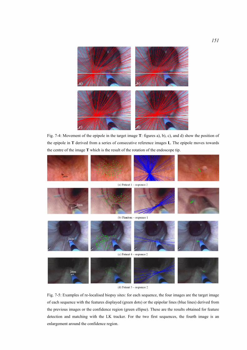
151
a) b)
c) d) Fig. 7-4: Movement of the epipole in the target image T: figures a), b), c), and d) show the position of
the epipole in T derived from a series of consecutive reference images Ii. The epipole moves towards
the centre of the image T which is the result of the rotation of the endoscope tip.
Fig. 7-5: Examples of re-localised biopsy sites: for each sequence, the four images are the target image
of each sequence with the features displayed (green dots) or the epipolar lines (blue lines) derived from
the previous images or the confidence region (green ellipse). These are the results obtained for feature
detection and matching with the LK tracker. For the two first sequences, the fourth image is an
enlargement around the confidence region.
152
The epipolar geometries of each pair of reference and target images were estimated
from sets of features detected with the LK tracker or with SIFT. In practice, the LK tracker
could track on average 100 features in the endoscopic images processed for this experiment
and it returned approximately 30% outliers. The SIFT usually returned 70 matches with 50%
outliers. The LK tracker has the advantage of tracking features through successive images
which constrains spatially the search for the matching features and guarantees, therefore, high
proportion and number of inliers. The SIFT does not constrain spatially the feature matching
and may return, therefore, more outliers than the LK tracker. Epipolar geometry is more
accurate when recovered from high proportion and number of inliers and the epipolar lines
derived from this geometry are, therefore, more accurate (Luong and Faugeras, 1996; Hartley
and Zisserman, 2004). As the epipolar lines used for the re-localisation could be more
accurate for the case of LK features, the re-localised biopsy sites were more accurate.
The more precise and accurate results were obtained for Patient 1 Sequence 2, Patient
2 Sequence 1, and Patient 3 Sequence 1 (Table 7-2 and Table 7-3). These sequences were
acquired without a miniprobe in the FOV. Therefore, the detected features were well
distributed over the oesophagus surface observed with the endoscope (Fig. 7-5 a)). They were
detected at various depths and along the curvature of the oesophagus. Such a good
distribution guarantees accurate epipolar lines as stated by Luong and Faugeras (1996).
Finally, the endoscope could move freely with wide translations and rotations. The resulting
epipolar lines subtended large angles (Fig. 7-5 a)) unlike those for the sequences acquired
with a miniprobe in the FOV (Fig. 7-5 b) and c)). The variety of directions is taken into
account in the uncertainty matrix Λp of the re-localised biopsy site for the cases where the
features have been detected and matched with the LK tracker. Large differences between the
line directions contribute to small ellipses (Fig. 7-5 a)) and, therefore, to small values of the
analytical precision. Also, accurate epipolar lines contributed to the high precision of the re-
localisation. Thus, the combination of a good distribution of the features over the observed
surface with a variety of directions of the epipolar lines helped reach high re-localisation
precisions for these 3 sequences.
For some of the sequences where a miniprobe was introduced in the endoscope FOV,
the values of analytical precision and accuracy were larger than for the other sequences. For
Patient 3 Sequence 2 and Patient 4 Sequence 2, for example, the FOV of the target image T
was bigger. The size of a pixel in the neighbourhood of the re-localised biopsy site and of the
ground truth was, therefore, larger for these sequences. The resulting accuracy was large.
Also, the re-localised biopsy site was computed from a set of epipolar lines that did not
153
subtend large angles (Fig. 7-5 c) and d)) and the resulting precision was, therefore, large for
the cases where the features were detected and matched with the LK tracker.
7.4 Conclusion
This chapter presented the results of the re-localisation method for endoscopic images
acquired on phantom and on patients. A re-localisation with N > 2 epipolar lines returns more
accurate results than with only 2 epipolar lines. Moreover, as the LK tracker tended to return
a greater proportion of inliers among the matched features than the SIFT, the epipolar lines
derived for the re-localisations tended to be more accurate, and the resulting re-localised
biopsy site was also more accurate. Nevertheless, matching SIFT features may be useful
when the camera field of view is obstructed by air/water bubbles or when the biopsy site
needs to be re-localised during a future examination using reference images acquired during a
previous examination. The next chapter presents a method to increase the proportion of
inliers among the SIFT features.

154
Chapter 8 Combination of an Electromagnetic Tracking
System with the Re-Localisation Method
8.1 Introduction
Fig. 8-1: Critical cases for a good performance of the LK tracker: two sequences of endoscopic images
aquired during a surveillance examination of Barrett’s Oesophagus (BO) are presented as examples.
For each sequence, 3 endoscopic images are extracted to illustrate the problems that may be
encountered during endoscopy. For sequence 1 and sequence 2, the oesophagus surface is interrogated
by optical biopsy (top row), air/water bubbles may obstruct the endoscope Field Of View (FOV) or the
endoscope may move too fast when the miniprobe is removed (middle row), and the endoscopic
images are clear again (bottom row).
155
The previous chapters introduced a method to re-localise a biopsy site in a target endoscopic
image T. This method makes use of epipolar lines derived from at least two previously
acquired endoscopic images Ii where the biopsy site location is known. Therefore, the
epipolar geometry formed between each pair of images Ii ↔ T needs to be recovered. Once
the biopsy site is re-localised, its uncertainty can be computed in order to provide the
endoscopist with a measure of the re-localisation precision and with the display of a
confidence region around the re-localised biopsy site in the target image T.
As presented in Chapter 3, the recovery of the epipolar geometry requires the
detection of features in the endoscopic images Ii and T and their matching for each pair Ii ↔
T. During a surveillance examination of Barrett’s Oesophagus (BO), the endoscopist may
manage to move the endoscope slowly, while keeping the biopsy site in the camera Field Of
View (FOV). In that case, the Lucas-Kanade (LK) tracker can be applied in order to detect
features in a first reference image Ii and in order to track them through the next images until
the target image T. However, in some situations, the camera FOV may be obstructed by
air/water bubbles or the endoscope tip may move too fast (Fig. 8-1). In these two cases, the
features are lost by the LK tracker and an alternative way of matching features is necessary.
This chapter aims to present and discuss a method to re-localise biopsy sites when the
features have been lost by the LK tracker. An ElectroMagnetic (EM) tracking system is used
to guide the process of feature matching. This method contributes to more accurate epipolar
lines and re-localised biopsy sites. A first experiment was done in order to assess the
accuracy of an EM tracking system in the conditions of an endoscopy. The results of this
experiment are presented. The results of a second experiment on a phantom demonstrate that
the EM tracking system helps increase the number and the proportion of good feature
matches and compute more accurate epipolar lines. Finally, the results of a third experiment
on excised porcine tissues show that more accurate re-localised biopsy sites can be computed
using the EM tracking system.
8.2 Re-localisation with an EM tracking system
8.2.1 Context, hypotheses, and description of an EM tracking system
The LK tracker may lose track of the features when air/water bubbles obstruct the FOV of the
endoscope camera, or when the camera moves too quickly. As discussed in Chapter 4, the
Scale Invariant Feature Transform (SIFT) features may be an alternative to the LK tracker in
these critical cases. Indeed, the features are detected independently in images Ii and T using
the scale-space representations of the images. For each detected feature, a descriptor is
computed. It is a vector which gives information about the distribution of the magnitude and
156
orientation of the gradients in the neighbourhood of the corresponding feature. Features are
matched by searching for the pair of descriptors in images Ii and T whose Euclidean distance
is minimal. Features, especially SIFT features, in endoscopic images correspond to blood
vessel junctions. As discussed in Chapter 4, junctions all look similar as do the descriptors
(Atasoy et al., 2009). This may create ambiguity when the SIFT features are matched and
result in a lot of mismatches or outliers. It is, therefore, necessary to guide spatially the
matching of SIFT features. For example, a rough knowledge of the relative positions between
the endoscope cameras can help determine a region in the target image where the correct
match of a feature in the reference image is likely to be.
An estimation of the endoscope camera movement can be given by positional sensors
such as an EM sensor mounted at the tip of the endoscope (Mori et al., 2005, 2007, and
2008). Mori et al. (2005, 2006, 2007, and 2008) built up hybrid systems combining
endoscopes, CT scanners, and EM tracking systems to track the positions and movement of
an endoscopic camera during a bronchoscopy procedure in a 3D reconstruction of the lumen
of the lung from a CT pre-operative image using registration of real endoscopic images with
virtual endoscopic images extracted from the 3D reconstruction. Given information about the
relative movement of the real camera from the EM sensor and a transformation from the real
camera coordinate system to the virtual camera coordinate system, the position of the virtual
camera could be updated in the virtual view and this position was used to initialise the image
registration algorithms for a refinement of the virtual camera position. In the case of biopsy
site re-localisation, the relative movement between endoscope cameras given by the EM
sensor can help identify a region in the target image where the match of a feature is.
An EM tracking system is made up of an emitter which generates electromagnetic
waves and of a sensor whose position and orientation are computed in the emitter coordinate
system (Fig. 8-2). The emitter is a box fixed next to the patient, for example. A coordinate
system (O, xem, yem, zem) is assigned to it and is used as a reference coordinate system for the
sensor. The sensor is made up of 3 coils that are arranged such that they form a coordinate
system (S, xS, yS, zS). The electromagnetic field is measured at the origin S of the sensor
coordinate system and the distance of S from the origin O of the emitter coordinate system
can be computed. Thus, the position S of the EM sensor is known in real-time in the emitter
coordinate system (O, xem, yem, zem). At position S, the orientations of the unit vectors of the
sensor coordinate system xS, yS, and zS in the emitter coordinate system are given by the
azimuth ψ, elevation θ, and roll Φ angles (Fig. 8-3). Thus, the rotational component of the
transformation matrix from the emitter coordinate system to the sensor coordinate system is
given by:
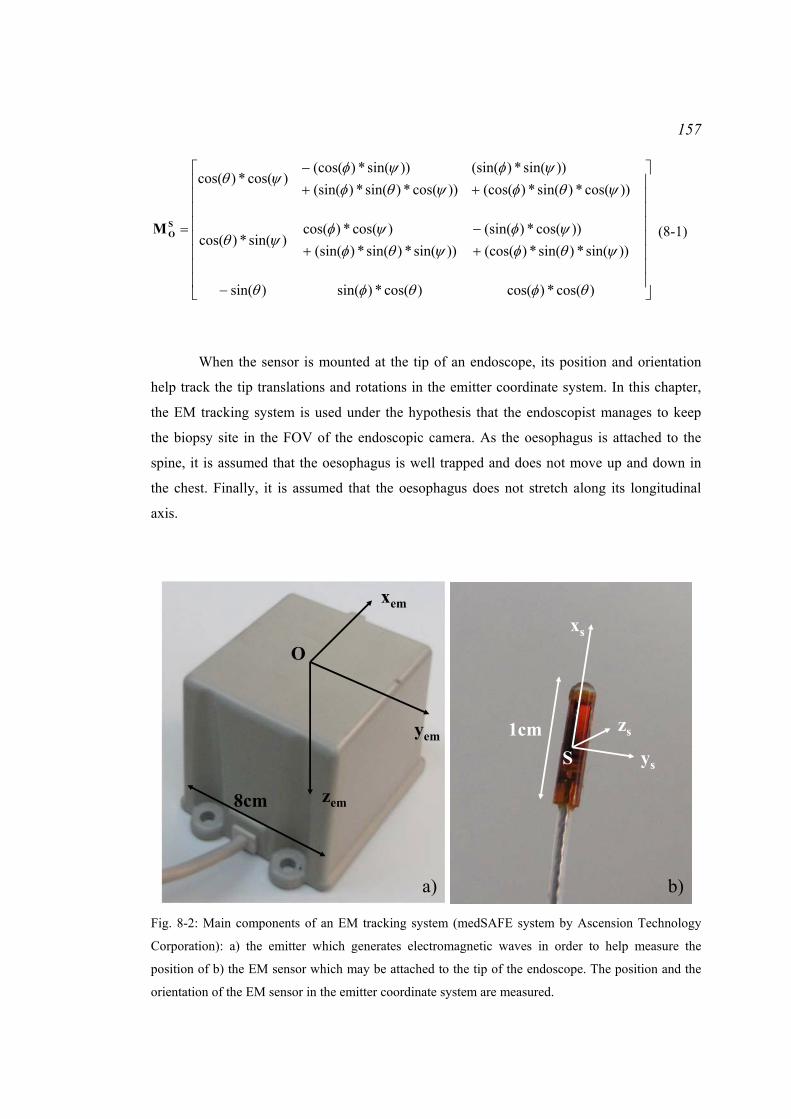
157
⎥⎥⎥⎥⎥⎥⎥⎥
⎦
⎤
⎢⎢⎢⎢⎢⎢⎢⎢
⎣
⎡
−
+−
+
++−
=
)cos(*)cos()cos(*)sin()sin(
))sin(*)sin(*)(cos())cos(*)(sin(
))sin(*)sin(*)(sin()cos(*)cos(
)sin(*)cos(
))cos(*)sin(*)(cos())sin(*)(sin(
))cos(*)sin(*)(sin())sin(*)(cos(
)cos(*)cos(
θφθφθ
ψθφψφ
ψθφψφ
ψθ
ψθφψφ
ψθφψφ
ψθ
SOM
(8-1)
When the sensor is mounted at the tip of an endoscope, its position and orientation
help track the tip translations and rotations in the emitter coordinate system. In this chapter,
the EM tracking system is used under the hypothesis that the endoscopist manages to keep
the biopsy site in the FOV of the endoscopic camera. As the oesophagus is attached to the
spine, it is assumed that the oesophagus is well trapped and does not move up and down in
the chest. Finally, it is assumed that the oesophagus does not stretch along its longitudinal
axis.
xem
xs
zs
ys
yem
zem
a) b)
O
S
8cm
1cm
Fig. 8-2: Main components of an EM tracking system (medSAFE system by Ascension Technology
Corporation): a) the emitter which generates electromagnetic waves in order to help measure the
position of b) the EM sensor which may be attached to the tip of the endoscope. The position and the
orientation of the EM sensor in the emitter coordinate system are measured.

158
xemyem
zem
Φ
θψ
yS
xS
zS
Fig. 8-3: Description of the EM sensor coordinate system (S, xS, yS, zS) in the EM emitter coordinate
system (O, xem, yem, zem) with spherical coordinates: the azimuth ψ, elevation θ, and roll Φ angles.
8.2.2 Combination of the EM tracking system with the re-localisation algorithm
A re-localised biopsy site p can be computed in a target image T by recovery of the epipolar
geometry formed by T with each of at least two reference images Ii that each show the site
under different viewpoints. The epipolar geometry formed by the pair of images Ii ↔ T is
represented algebraically using the fundamental matrix ( )TIF ,i:
( ) ( )[ ] ( ) ( ) ⋅⋅⋅⎥⎥⎥
⎦
⎤
⎢⎢⎢
⎣
⎡
−−
−⋅=⋅⋅⋅= 1-
,
12
13
23tr-1-
,,tr-
,
00
0KRKKRtKF TITITITI iiii
tttt
tt
(8-2)
K is the intrinsic matrix linking the endoscope camera coordinate system with the 2D image
plane coordinate system. K can be assumed constant during endoscopy investigations and
recovered from a calibration procedure (Bouguet, 2004). The fundamental matrix ( )TIF ,i can
be computed either with computer vision algorithms as presented in Chapter 3 or with the
EM tracking system when the sensor is mounted at the tip of the endoscope camera or with a
combination of the two previous methods.
The hybrid method for biopsy site re-localisation detects SIFT features and estimates
the fundamental matrix from the EM tracking system referred to ( ( )TIF ,i)EM for each pair of
images Ii ↔ T. The fundamental matrix ( ( )TIF ,i)EM is used to increase the percentage and
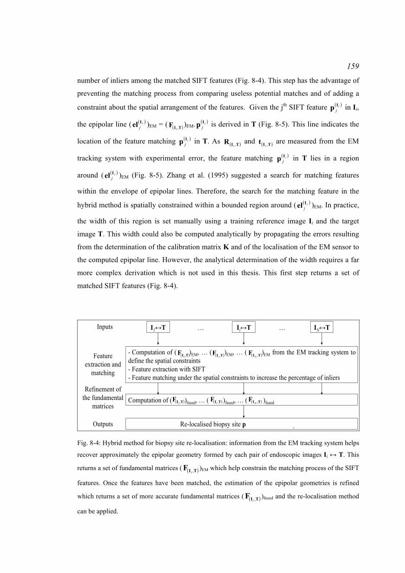
159
number of inliers among the matched SIFT features (Fig. 8-4). This step has the advantage of
preventing the matching process from comparing useless potential matches and of adding a
constraint about the spatial arrangement of the features. Given the jth SIFT feature ( )ijIp in Ii,
the epipolar line ( ( )ijIel )EM = ( ( )TIF ,i
)EM. ( )ijIp is derived in T (Fig. 8-5). This line indicates the
location of the feature matching ( )ijIp in T. As ( )TIR ,i
and ( )TIt ,i are measured from the EM
tracking system with experimental error, the feature matching ( )ijIp in T lies in a region
around ( ( )ijIel )EM (Fig. 8-5). Zhang et al. (1995) suggested a search for matching features
within the envelope of epipolar lines. Therefore, the search for the matching feature in the
hybrid method is spatially constrained within a bounded region around ( ( )ijIel )EM. In practice,
the width of this region is set manually using a training reference image Ii and the target
image T. This width could also be computed analytically by propagating the errors resulting
from the determination of the calibration matrix K and of the localisation of the EM sensor to
the computed epipolar line. However, the analytical determination of the width requires a far
more complex derivation which is not used in this thesis. This first step returns a set of
matched SIFT features (Fig. 8-4).
Re-localised biopsy site p and confidence region
…I1↔T
- Computation of ( )EM, … ( )EM, … ( )EM from the EM tracking system to define the spatial constraints- Feature extraction with SIFT- Feature matching under the spatial constraints to increase the percentage of inliers
…Inputs
Feature extraction and
matching
Refinement of the fundamental
matrices
Outputs
Ii↔T IN↔T
Computation of ( )fused, … ( )fused, … ( )fused
( )TIF ,i( )TIF ,1 ( )TIF ,N
( )TIF ,1 ( )TIF ,i ( )TIF ,N
Fig. 8-4: Hybrid method for biopsy site re-localisation: information from the EM tracking system helps
recover approximately the epipolar geometry formed by each pair of endoscopic images Ii ↔ T. This
returns a set of fundamental matrices ( ( )TIF ,i)EM which help constrain the matching process of the SIFT
features. Once the features have been matched, the estimation of the epipolar geometries is refined
which returns a set of more accurate fundamental matrices ( ( )TIF ,i)fused and the re-localisation method
can be applied.
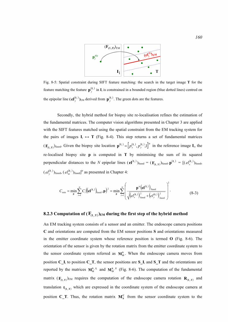
160
I iI i T
pj(elj )EM
(F( ,T))EM
(Ii)
Ii
(Ii)
Fig. 8-5: Spatial constraint during SIFT feature matching: the search in the target image T for the
feature matching the feature ( )ijIp in Ii is constrained in a bounded region (blue dotted lines) centred on
the epipolar line ( ( )ijIel )EM derived from ( )i
jIp . The green dots are the features.
Secondly, the hybrid method for biopsy site re-localisation refines the estimation of
the fundamental matrices. The computer vision algorithms presented in Chapter 3 are applied
with the SIFT features matched using the spatial constraint from the EM tracking system for
the pairs of images Ii ↔ T (Fig. 8-4). This step returns a set of fundamental matrices
( ( )TIF ,i)fused. Given the biopsy site location ( ) ( ) ( )[ ] tr
1,, iiiyx pp IIIp = in the reference image Ii, the
re-localised biopsy site p is computed in T by minimising the sum of its squared
perpendicular distances to the N epipolar lines ( ( )iIel )fused = ( ( )TIF ,i)fused. ( )iIp = [( ( )i
xel I )fused,
( ( )iyel I )fused, ( ( )i
mel I )fused]tr as presented in Chapter 4:
( )( )( )( )( )
( )( ) ( )( )∑∑==
⋅⎟⎟⎟
⎠
⎞
⎜⎜⎜
⎝
⎛
+==
N
iyx
N
ii
ii
i
i
elelCC
1
2
2
fused
2
fused
fusedtr
1
2fusedmin min,min
II
I
p
I
p
elppel
(8-3)
8.2.3 Computation of ( ( )TIF ,i)EM during the first step of the hybrid method
An EM tracking system consists of a sensor and an emitter. The endoscope camera positions
C and orientations are computed from the EM sensor positions S and orientations measured
in the emitter coordinate system whose reference position is termed O (Fig. 8-6). The
orientation of the sensor is given by the rotation matrix from the emitter coordinate system to
the sensor coordinate system referred as SOM . When the endoscope camera moves from
position C_Ii to position C_T, the sensor positions are S_Ii and S_T and the orientations are
reported by the matrices iISOM _ and TS
OM _ (Fig. 8-6). The computation of the fundamental
matrix ( ( )TIF ,i)EM requires the computation of the endoscope camera rotation ( )TIR ,i
and
translation ( )TIt ,i which are expressed in the coordinate system of the endoscope camera at
position C_T. Thus, the rotation matrix CSM from the sensor coordinate system to the

161
endoscope camera coordinate system has to be determined. By mechanical design, these two
coordinate systems are fixed relative to each other, and CSM is determined during a
calibration procedure by recording the EM sensor data and the endoscope camera images of a
calibration grid while the endoscope positions and orientations vary.
The translation ( )TIt ,i is computed from the EM sensor position S_Ii and S_T
measured in the emitter coordinate system. The translation has to be computed in the EM
sensor coordinate system at position S_T, first, using the rotation matrix TSOM _ . The resulting
vector is expressed in the camera coordinate system at position C_T, secondly, using the
rotation matrix CSM . Therefore, ( )TIt ,i
is computed as follows:
( ) ( ) ( ) ( )iiISTSMMt TS
OCSTI __.. 1_1
, −=−−
. (8-4)
The matrix ( )TIR ,i is the relative rotation from one endoscope camera position to
another position. It is given directly by the EM sensor and it can be decomposed as a product
of rotations from the EM sensor coordinate system to the EM emitter coordinate system SOM
at positions S_Ii and S_T:
( ) ( ) ( ) CS
ISO
TSO
CSTI MMMMR ... _1_1
,i
i
−−= . (8-5)
8.3 Experiments and results
This section describes a set of experiments to test how well the hybrid method performs to
derive the epipolar lines necessary for the re-localisation. The performance depends on:
• The accuracy of the EM tracking system to determine the position of the endoscope.
O
Emitter coordinate system
Sensor coordinate system
Camera coordinate system
CS
Endoscope
SOM
CSM
Fig. 8-6: Relations between the coordinate systems of the camera, of the EM sensor, and of the EM
emitter.

162
• The matched features between the reference image Ii and the target image T. As
discussed in Chapter 4 in section ‘4.3.2 Experiment: number of matches for the
computation of the fundamental matrix’ and as stated by Luong and Faugeras (1996)
and Hartley and Zisserman (2004), accurate epipolar geometry is recovered when
there are a lot of well matched features or inliers (Luong and Faugeras, 1996; Hartley
and Zisserman, 2004).
• The endoscope camera. If the resolution is high, the blood vessels are pictured with
more details in the acquired endoscopic images. The vessels may also appear with a
better contrast. Features may be better detected in these conditions.
• The illumination of the tissue. If the oesophagus structure is well illuminated, the
vessels are visible in the whole image and the detected features are spread well over
the endoscopic image.
The experiments consisted of first assessing the error with which the EM tracking
system measures the displacement of the EM sensor. Secondly, the experiments consisted of
studying the error of the positioning of the epipolar lines derived with the re-localisation
system. The last experiment consisted of testing the method on excised organs from pigs.
8.3.1 Experiment 1: error of an EM tracking system for the determination of the
displacement and of the orientation of the EM sensor
Fig. 8-7: Experimental setup: a) the EM sensor was mounted at the tip of the endoscope; b) the
endoscope and the EM sensor were clamped by a probe holder that could be moved in various
directions; c) the phantom was a carton box in which holes were drilled every centimetre.
163
An EM tracking system can be used to measure the endoscope camera movement.
Therefore, the error of the measurement of the orientation and of the relative distance
between two positions of the EM sensor had to be estimated.
8.3.1.1 Materials and method
Hummel et al. (2005) did an intensive study of the accuracy of various EM tracking systems.
They designed a phantom which was a plexiglass board with holes drilled at regular
distances. The EM sensor was inserted in each hole. The positions and orientations of the
sensor were measured. Hummel et al. (2005) compared the measured distances between two
neighbouring holes and the measured angles to the actual distance on the phantom and to the
actual change of angle. They also assessed the accuracy of the EM sensor in presence of
various metals which can distort the electromagnetic signal.
In this chapter, the experiment aimed to assess the accuracy of the EM tracking
system in the context of an endoscopy. The EM tracking system was the medSAFE system by
Ascension Technology Corporation and the EM sensor had 6 degrees of freedom. The
experiment was inspired from those presented in Hummel et al. (2005). An EM sensor was
mounted at the tip of an endoscope since this is the way the EM tracking system is used in the
hybrid method (Fig. 8-7 a)). The endoscope contains metallic parts that can distort the signal
measured by the EM sensor. The endoscope and the EM sensor were held by a probe holder
which helped move them manually with a controlled movement (Fig. 8-7 b)). The phantom
was similar to Hummel et al. (2005) phantom. Hundred holes were drilled every centimetre
(d0 = 1cm) in a carton board (Fig. 8-7 c)).
The experiment consisted of moving the endoscope and the EM sensor with the probe
holder from holes to holes without changing the orientation. The EM sensor position and
orientation were measured in the EM emitter coordinate system. For each hole, its distance di
from each of its 4 neighbours was computed and compared to d0. As suggested by Hummel et
al. (2005), the Root Mean Squared (RMS) error of the difference between the measured
distances di and the exact distance d0 was computed in order to assess the error resulting from
an estimation of the displacement of an endoscope camera with an EM tracking system:
( )∑=
−⋅−
=n
ii dd
1n 1
20error
1RMS . (8-6)
where n is the total number of distances compared. The maximum, minimum, and mean error
was computed. Furthermore, due to the nature of the movement of the probe holder, the
changes of orientations of the EM sensor should be null. The values of the azimuth ψ0,
elevation θ0, and roll Φ0 angles at the position of the hole scanned first with the EM sensor

164
were measured and used as the ground truth angles. The values of ψi, θi, and Φi angles for the
99 other positions were measured and compared to the ground truth. Therefore, the RMS
errors of (ψi - ψ0), of (θi - θ0), and of (Φi - Φ0) were computed as well as their maximum,
minimum, and mean errors. For this experiment, the board was positioned at a distance of
approximately 50cm from the EM emitter which is a reasonable distance during clinical
practice on the patient. Hundred holes were drilled because that is a significant number for
the estimation of the RMS error. Finally, the distance between two holes was 1cm such that
the distance along one line corresponded to the movement amplitude of the probe holder.
8.3.1.2 Results and discussion
The results are presented in Table 8-1. On average, the displacement and the orientation of
the EM sensor were measured with an error of approximately 1mm and less than 3 degrees.
As the EM sensor was placed in contact with the table supporting the phantom when it was
inserted into the hole, the difference of elevation from one hole to another was smaller than
for the other angles. Thus, the RMS error, maximum error, and mean error were smaller. The
insertion of the sensor into the hole could create small rotations of the sensor and the
resulting errors for the azimuth and roll angles were larger than for the elevation angle.
Finally, the variations of the measurements could be due to the noise generated by devices or
metal objects in the neighbourhood which use or carry large amounts of electrical current that
vary over time or to the internal noise of the EM tracking system (Hummel et al., 2005).
These sources of noise came from the endoscope and the metallic tables in the room where
the experiment was run.
The accuracy of the measurements from the EM sensor has an influence on the
accuracy of the fundamental matrix estimated from the EM tracking system. The next
experiments study the accuracy of the epipolar lines computed with the hybrid method and
used for the re-localisation.
Table 8-1: Results of the errors between the measured distances and the exact distance (in millimetres)
and between the angles (in degrees):
di – d0 (mm) ψi – ψ0 (degrees) θi – θ0 (degrees) Φi – Φ0 (degrees)
Maximum 2.034 9.582 4.183 10.443
Minimum 0.012 0.042 0 0.016
Mean 0.778 2.276 0.959 3.250
RMSerror 0.935 3.766 1.294 4.083

165
8.3.2 Experiment 2: error of the positioning of the epipolar lines derived with the
re-localisation system
This experiment aimed to study the contribution of the EM tracking system to the feature
matching and to the computation of the epipolar lines derived for the re-localisation of a
biopsy site. This experiment was run on a phantom with an EM sensor attached to the tip of a
fibered endoscope. As the transformation matrix CSM which relates the EM sensor coordinate
system to the endoscope camera coordinate system was unknown, a preliminary step was the
determination of CSM during a registration procedure. Thus, this part is organised as follows:
• First, the experimental setup is presented.
• Secondly, the procedure for the study of the error of the positioning of an epipolar
line is presented.
• Finally, the results of the study are discussed.
8.3.2.1 Methods and materials
2.5 cm2.5 cm
CCD camera
Endoscope
Gastroscope tip
EM sensor
x-axis
y-axis
z-axis
a)
b)
c)
d)
e)
Rigid tube
Fig. 8-8: Experimental setup: a) the phantom was a rigid tube of diameter 2.5cm; b) a texture
mimicking a vascular network was printed onto a piece of paper and stuck to the inner surface of the
tube and rolled into the phantom; c) a fibered endoscope was used in combination with a CCD camera
placed at the end of the fibered endoscope; d) the EM sensor was attached to the tip of the endoscope;
e) the tip of the endoscope and the EM sensor were held with a probe holder that could move along 3
orthogonal directions.

166
8.3.2.1.1 Experimental setup
The experimental setup was designed such that it reproduced the conditions of a gastroscopic
examination. As the oesophagus is positioned next to the spine and physically constrained
between the trachea and the lungs, it was assumed that the oesophagus is well fixed in the
patient’s chest and does not stretch. According to the sequences acquired on patients, the
endoscopist manages to maintain the endoscope on the central axis of the oesophagus which
is why the movement of the endoscope camera in these experiments was along this axis. Such
an observation was made also in Mori et al. (2007) during bronchoscopy examinations.
A physical phantom was built from a 2.5cm diameter rigid tube, which corresponds
approximately to the diameter of an oesophagus (Fig. 8-8 a)). A synthetic texture was rolled
into the tube. It had to realistically represent the pattern of the oesophagus walls. Real vessels
could be described as lines that intersect. Their thickness was approximately 0.3mm
according to inspection of real endoscopic images. Therefore, 0.3mm thick lines were
generated digitally and printed out on a piece of white paper. The lines were positioned and
orientated by random selections of a position and orientation within the image (Fig. 8-8 b)).
A fibered endoscope was used for the acquisition of endoscopic images. The inside
of the phantom was illuminated with a Xenon lamp, and a CCD camera was placed at the end
of the bundle of fibres for image recording (Fig. 8-8 c)). There were thousands of fibres
which were arranged in a honeycomb pattern. A relay lens to allow eyepiece images to be
focused onto the chosen CCD camera was placed between the camera and the end of the
bundle of fibres. Acquired images had a resolution of approximately 1600pixels x
1200pixels. Images of such a resolution can be obtained during real endoscopy by using
adequate video image grabbers. An EM sensor was attached to the tip of the endoscope in
order to record the rotations and translations of the tip (Fig. 8-8 d)). The endoscope tip will be
called the endoscope camera from now on. The endoscope camera was inserted into the
phantom. It was attached to a probe holder in order to control its movement and in order to
measure precisely the actual translation of the endoscope camera (Fig. 8-8 e)).
Before endoscopic images and EM tracking data were acquired, a procedure was run
in order to register the endoscope camera coordinate system to the sensor coordinate system
and in order to determine CSM which is necessary for the estimation of the epipolar geometry
from the EM tracking system. This was achieved by acquiring a series of endoscopic images
of a calibration pattern seen from different viewpoints of the endoscope camera. For each
camera pose, the positional data of the EM sensor were recorded. The method was described
by Tsai and Lenz (1989) and a Matlab implementation (Matlab, R14, The Mathworks Ltd,
Cambridge, UK) by Wengert et al. (2006) was used to determine the transformation CSM .
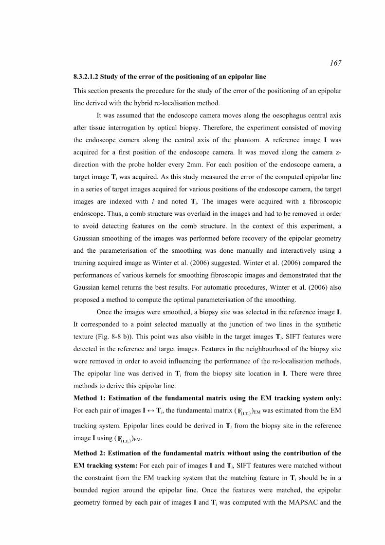
167
8.3.2.1.2 Study of the error of the positioning of an epipolar line
This section presents the procedure for the study of the error of the positioning of an epipolar
line derived with the hybrid re-localisation method.
It was assumed that the endoscope camera moves along the oesophagus central axis
after tissue interrogation by optical biopsy. Therefore, the experiment consisted of moving
the endoscope camera along the central axis of the phantom. A reference image I was
acquired for a first position of the endoscope camera. It was moved along the camera z-
direction with the probe holder every 2mm. For each position of the endoscope camera, a
target image Ti was acquired. As this study measured the error of the computed epipolar line
in a series of target images acquired for various positions of the endoscope camera, the target
images are indexed with i and noted Ti. The images were acquired with a fibroscopic
endoscope. Thus, a comb structure was overlaid in the images and had to be removed in order
to avoid detecting features on the comb structure. In the context of this experiment, a
Gaussian smoothing of the images was performed before recovery of the epipolar geometry
and the parameterisation of the smoothing was done manually and interactively using a
training acquired image as Winter et al. (2006) suggested. Winter et al. (2006) compared the
performances of various kernels for smoothing fibroscopic images and demonstrated that the
Gaussian kernel returns the best results. For automatic procedures, Winter et al. (2006) also
proposed a method to compute the optimal parameterisation of the smoothing.
Once the images were smoothed, a biopsy site was selected in the reference image I.
It corresponded to a point selected manually at the junction of two lines in the synthetic
texture (Fig. 8-8 b)). This point was also visible in the target images Ti. SIFT features were
detected in the reference and target images. Features in the neighbourhood of the biopsy site
were removed in order to avoid influencing the performance of the re-localisation methods.
The epipolar line was derived in Ti from the biopsy site location in I. There were three
methods to derive this epipolar line:
Method 1: Estimation of the fundamental matrix using the EM tracking system only:
For each pair of images I ↔ Ti, the fundamental matrix ( ( )iTIF , )EM was estimated from the EM
tracking system. Epipolar lines could be derived in Ti from the biopsy site in the reference
image I using ( ( )iTIF , )EM.
Method 2: Estimation of the fundamental matrix without using the contribution of the
EM tracking system: For each pair of images I and Ti, SIFT features were matched without
the constraint from the EM tracking system that the matching feature in Ti should be in a
bounded region around the epipolar line. Once the features were matched, the epipolar
geometry formed by each pair of images I and Ti was computed with the MAPSAC and the

168
nonlinear optimisation. The epipolar lines were derived in T from the biopsy site locations in
the image I.
Method 3: Estimation of the fundamental matrix using the contribution of the EM
tracking system: This was the method of the whole re-localisation presented in Chapter 8.
For each pair of images I ↔ Ti, the fundamental matrix ( ( )iTIF , )EM was estimated from the EM
tracking system. For each image I and Ti, SIFT features were matched with the spatial
constraint. A training image was used to set the value of the width of the bounded region. The
epipolar lines were derived after refinement of the epipolar geometry with MAPSAC and a
nonlinear optimisation over the matched features. Epipolar lines were derived in Ti from the
biopsy site locations in the image I.
The distance from the true location of the biopsy site in Ti to the epipolar line was
computed in order to assess the error of the positioning of the epipolar line. This distance was
measured in pixels and in millimetres. It was assumed that the epipolar line was sufficiently
close to the biopsy site to approximate the 2D distance as representative of the real 3D
distance. The measures in pixels were converted in millimetres using information about the
actual thickness of the lines as a scale. Besides, according to real patient data, the contrast
between the vessels and the homogeneous tissue was defined as (Imax - Imin)/(Imax + Imin) where
Imax is the intensity of the paper and Imin the intensity of the line and could vary from 0 to 1.
The contrast of the vessels in the endoscopic images decreased with their distances from the
camera as the illumination got poorer. The contrast of the vessels also changed from one
patient to another. For some acquired sequences, the vessels had a low contrast with the
tissue. Thus, this experiment was repeated for several synthetic textures whose straight lines
had a contrast of first 0.5, secondly 0.3, and thirdly 0.2. In the acquired endoscopic images,
the lines appeared with weaker contrasts, still varying between 0 and 1.
8.3.2.2 Results and discussion
The results of the distances between the epipolar lines and a biopsy site location are presented
in Table 8-2, Table 8-3, and Table 8-4.

169 Table 8-2: Errors of the epipolar lines for various camera positions: contrast = 0.5
(28.
86 ;
0.65
)(5
.40
; 0.1
0)(1
.80
; 0.0
3)(3
.65
; 0.0
6)(3
.96
; 0.0
6)E
rror
(pix
els ;
mm
)
36%
30%
56%
74%
65%
Perc
enta
ge o
f in
liers
2123
5572
83N
umbe
r of
inlie
rs
5876
9897
128
Num
ber
of m
atch
es
Met
hod
3
(132
.97
; 2.9
7)(2
2.46
; 0.
43)
(13.
94 ;
0.22
)(4
.12
; 0.0
7)(3
.16
; 0.0
5)E
rror
(pix
els ;
mm
)
40%
44%
53%
77%
61%
Perc
enta
ge o
f in
liers
2635
4868
78N
umbe
r of
inlie
rs
6579
9188
127
Num
ber
of m
atch
es
Met
hod
2
(126
.75
; 2.8
3)(1
07.6
7 ;
2.04
)(8
4.21
; 1.
35)
(50.
87 ;
0.85
)(3
0.31
; 0.
45)
Err
or (p
ixel
s ; m
m)
Met
hod
1
I ↔T
510
mm
I ↔T
48m
mI ↔
T3
6mm
I ↔T
24m
mI ↔
T1
2 m
mC
amer
a di
spla
cem
ent
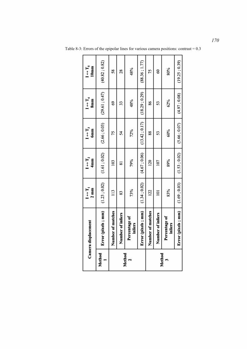
170 Table 8-3: Errors of the epipolar lines for various camera positions: contrast = 0.3
(19.
25 ;
0.39
)(4
.97
; 0.0
8)(5
.66
; 0.0
7)(1
.53
; 0.0
2)(1
.69
; 0.0
3)E
rror
(pix
els ;
mm
)
80%
62%
60%
89%
83%
Perc
enta
ge o
f in
liers
6053
5310
710
1N
umbe
r of
inlie
rs
7586
8812
012
2N
umbe
r of
mat
ches
Met
hod
3
(88.
36 ;
1.77
)(1
8.29
; 0.
29)
(13.
42 ;
0.17
)(4
.67
; 0.0
6)(1
.34
; 0.0
2)E
rror
(pix
els ;
mm
)
48%
48%
72%
79%
73%
Perc
enta
ge o
f in
liers
2833
5481
83N
umbe
r of
inlie
rs
5869
7510
311
3N
umbe
r of
mat
ches
Met
hod
2
(40.
82 ;
0.82
)(2
9.61
; 0.
47)
(2.6
6 ; 0
.03)
(1.6
1 ; 0
.02)
(1.2
3 ; 0
.02)
Err
or (p
ixel
s ; m
m)
Met
hod
1
I ↔T
510
mm
I ↔T
48m
mI ↔
T3
6mm
I ↔T
24m
mI ↔
T1
2 m
mC
amer
a di
spla
cem
ent

171 Table 8-4: Errors of the epipolar lines for various camera positions: contrast = 0.2
(13.
44 ;
0.22
)(1
6.50
; 0.
22)
(8.2
8 ; 0
.12)
(7.2
8 ; 0
.10)
Err
or (p
ixel
s ; m
m)
51%
43%
89%
88%
Perc
enta
ge o
f in
liers
5063
111
132
Num
ber
of in
liers
9912
312
515
0N
umbe
r of
mat
ches
Met
hod
3
(44.
84 ;
0.74
)(1
2.18
; 0.
16)
(20.
64 ;
0.31
)(9
.63
; 0.1
4)E
rror
(pix
els ;
mm
)
42%
40%
52%
65%
Perc
enta
ge o
f in
liers
3937
5677
Num
ber
of in
liers
9393
104
118
Num
ber
of m
atch
es
Met
hod
2
(30.
79 ;
0.51
)(2
3.53
; 0.
31)
(15.
50 ;
0.23
)(9
.31
; 0.1
3)E
rror
(pix
els ;
mm
)M
etho
d 1
I ↔T
48m
mI ↔
T3
6mm
I ↔T
24m
mI ↔
T1
2 m
mC
amer
a di
spla
cem
ent

172
For Method 1, the error of the positioning of the epipolar line increased when the
displacement of the endoscope camera was larger. First, the camera displacement was
measured by the EM sensor in the EM emitter coordinate system. The first experiment
showed that the displacement might be estimated with an error varying from 0.0012mm to
2.034mm. During the second experiment, the EM sensor measured, for example, a
displacement of 1.6mm instead of 2mm. This error affects the matrix [ ( )iTIt , ] used for the
estimation of the fundamental matrix ( ( )iTIF , )EM from the EM tracking system. It propagates to
the epipolar line. Secondly, ( )iTIR , and [ ( )iTIt , ] were computed with the measures from the EM
sensor and with the transformation matrix CSM from the EM sensor coordinate system to the
camera coordinate system. CSM was found by registration of the coordinate systems, but this
measurement includes error from the EM tracking system. Indeed, the registration consisted
of moving the endoscope with the EM sensor at the tip to various positions and acquiring
endoscopic images and EM sensor data for each position. The camera rotation and translation
were both computed from the images and measured from the EM sensor with experimental
error in order to register the camera coordinate system with the EM sensor coordinate system.
Thus, the error of the measurements with the EM sensor in combination with the error of the
computation of CSM could be responsible for the error of the position of the epipolar line in
Ti (Fig. 8-9, Fig. 8-10, and Fig. 8-11). The error of the measurement of the EM sensor
increased when the displacement was larger which is why the lines were further away from
the biopsy site for displacements of 8mm than for displacements of 2mm.
Fig. 8-9: Epipolar geometries recovered from the EM sensor for a contrast of 0.5 for a displacement of
2mm (a), 4mm (b), and 8mm (c): the set of images at the bottom row shows in image Ti the epipolar
line derived from the biopsy site in image I (red line) and from the epipolar geometry computed with
the EM tracking system only (top row). It also shows the ground-truth position of the biopsy site
(green point).
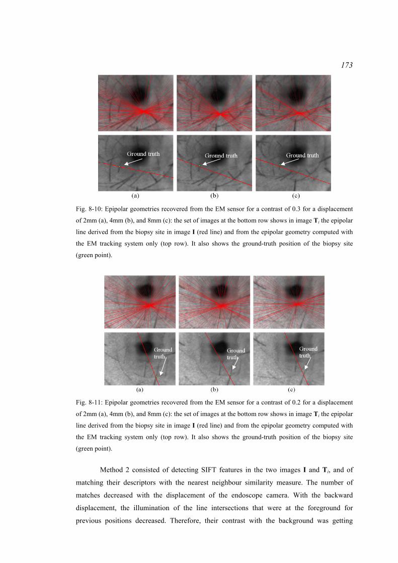
173
Fig. 8-10: Epipolar geometries recovered from the EM sensor for a contrast of 0.3 for a displacement
of 2mm (a), 4mm (b), and 8mm (c): the set of images at the bottom row shows in image Ti the epipolar
line derived from the biopsy site in image I (red line) and from the epipolar geometry computed with
the EM tracking system only (top row). It also shows the ground-truth position of the biopsy site
(green point).
Fig. 8-11: Epipolar geometries recovered from the EM sensor for a contrast of 0.2 for a displacement
of 2mm (a), 4mm (b), and 8mm (c): the set of images at the bottom row shows in image Ti the epipolar
line derived from the biopsy site in image I (red line) and from the epipolar geometry computed with
the EM tracking system only (top row). It also shows the ground-truth position of the biopsy site
(green point).
Method 2 consisted of detecting SIFT features in the two images I and Ti, and of
matching their descriptors with the nearest neighbour similarity measure. The number of
matches decreased with the displacement of the endoscope camera. With the backward
displacement, the illumination of the line intersections that were at the foreground for
previous positions decreased. Therefore, their contrast with the background was getting

174
weaker (Fig. 8-12). As SIFT requires setting a threshold for the contrast, the line intersections
were not necessarily detected as features. Decreasing the threshold, while the endoscope
camera moved backwards, could be a solution to increase the number of detected features and
of matches in I and Ti. During the experiment, this threshold was set at a low value in order
to detect features at the line intersections with a weak contrast. However, when the threshold
was set at a low value, the neighbourhood of the features was more blurred and the
descriptors of the detected features could become different as the endoscope camera moved
backwards (Fig. 8-13). For these two reasons, there was a risk of finding two descriptors in I
and Ti that were very similar while they corresponded to two different anatomical points.
This could result in a greater number of outliers among the feature matches when the
endoscope camera moved backwards. As the number of outliers increased, a lot of tests for
the estimation of the fundamental matrix with the MAPSAC were required with Method 2 in
order to determine accurate epipolar geometry.
Method 3 showed the same variations as Method 2 for the feature matching.
However, the number of matches and of inliers was higher than that for Method 2 (Table 8-2,
Table 8-3, and Table 8-4). As a spatial constraint was imposed by the epipolar lines, each
descriptor was compared only with the descriptors that were within the epipolar band (Fig.
8-14). This helped avoid matching two descriptors that were very similar although they
corresponded to two features that did not represent the same anatomical point. Not only did
the spatial constraint help find the correct matching feature, but it increased also the number
of detected inliers (Fig. 8-15). A match is not simply defined by a threshold on the Euclidean
distance between SIFT descriptors. A feature matches its nearest Euclidean neighbour if and
only if the ratio of the Euclidean distances with respectively the first and second nearest
neighbours is greater than a fixed threshold. The spatial constraint from the EM tracker
excludes gross matching errors. The first neighbour will more likely produce the correct
match. As the criterion is then the distance ratio, the matching leads to an increase in the
number of inliers. For example, as line intersections repeat within an endoscopic image,
multiple descriptors could match equally a descriptor in the reference image. The matching
without spatial constraint could return a wrong matching or no matching while the spatial
constraint returned the correct match (Fig. 8-15). The percentage of inliers was also higher
especially for large displacements, for example for a contrast of 0.3 for the pairs of images I
and T2, I and T4, and I and T5, or for a contrast of 0.2 for the pairs of images I and T4 (Table
8-3, and Table 8-4). A high percentage of inliers is important as it reduces the number of
estimations of MAPSAC necessary to find an accurate fundamental matrix.
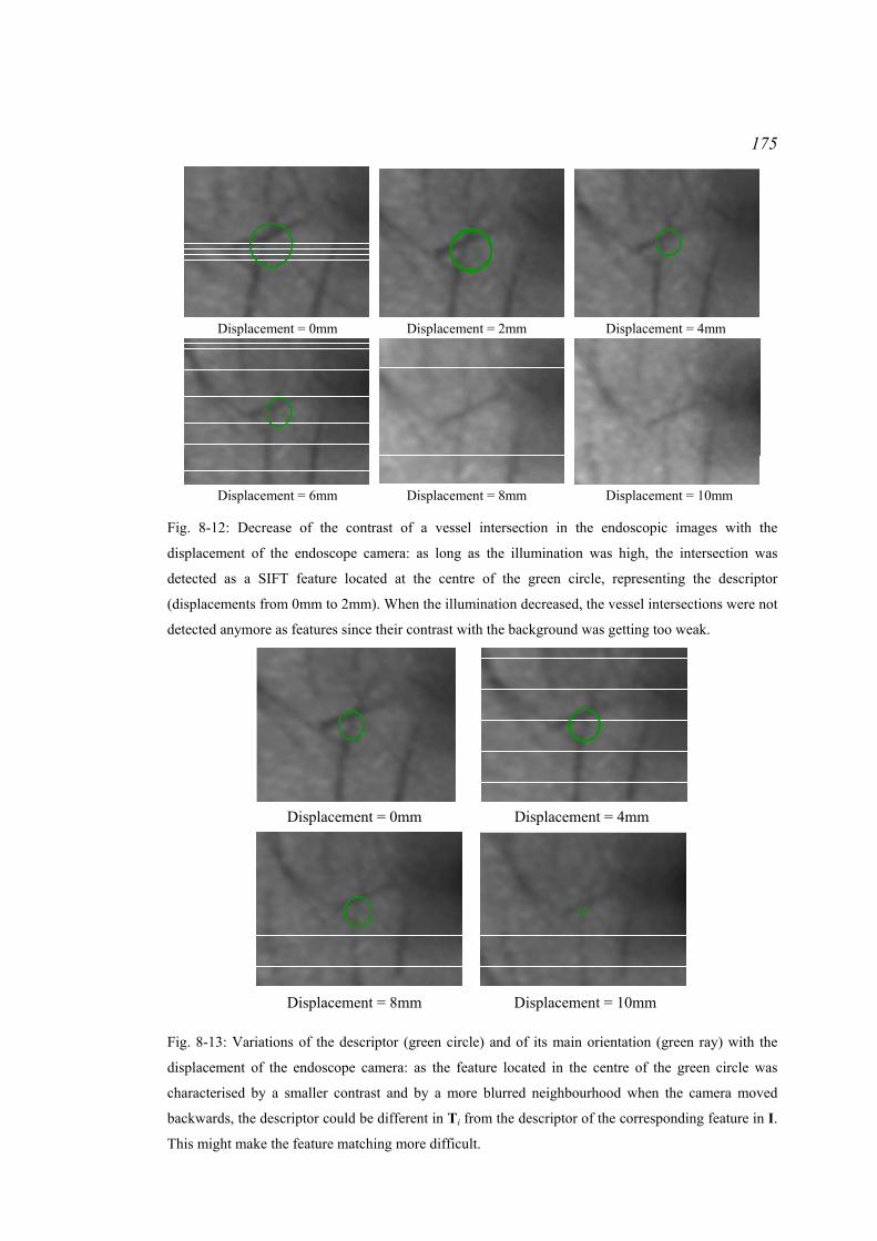
175
Displacement = 0mm Displacement = 2mm Displacement = 4mm
Displacement = 6mm Displacement = 8mm Displacement = 10mm Fig. 8-12: Decrease of the contrast of a vessel intersection in the endoscopic images with the
displacement of the endoscope camera: as long as the illumination was high, the intersection was
detected as a SIFT feature located at the centre of the green circle, representing the descriptor
(displacements from 0mm to 2mm). When the illumination decreased, the vessel intersections were not
detected anymore as features since their contrast with the background was getting too weak.
Displacement = 0mm Displacement = 4mm
Displacement = 8mm Displacement = 10mm
Fig. 8-13: Variations of the descriptor (green circle) and of its main orientation (green ray) with the
displacement of the endoscope camera: as the feature located in the centre of the green circle was
characterised by a smaller contrast and by a more blurred neighbourhood when the camera moved
backwards, the descriptor could be different in Ti from the descriptor of the corresponding feature in I.
This might make the feature matching more difficult.
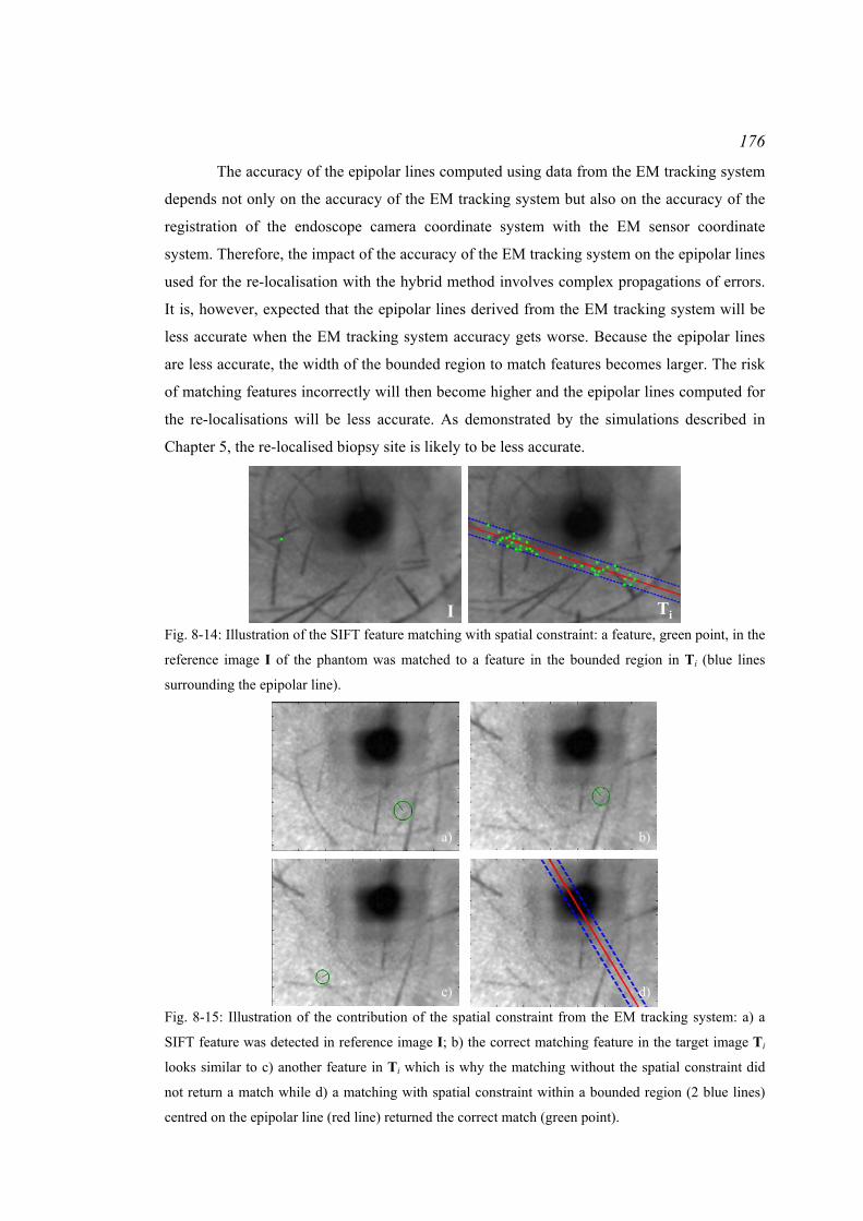
176
The accuracy of the epipolar lines computed using data from the EM tracking system
depends not only on the accuracy of the EM tracking system but also on the accuracy of the
registration of the endoscope camera coordinate system with the EM sensor coordinate
system. Therefore, the impact of the accuracy of the EM tracking system on the epipolar lines
used for the re-localisation with the hybrid method involves complex propagations of errors.
It is, however, expected that the epipolar lines derived from the EM tracking system will be
less accurate when the EM tracking system accuracy gets worse. Because the epipolar lines
are less accurate, the width of the bounded region to match features becomes larger. The risk
of matching features incorrectly will then become higher and the epipolar lines computed for
the re-localisations will be less accurate. As demonstrated by the simulations described in
Chapter 5, the re-localised biopsy site is likely to be less accurate.
I Ti Fig. 8-14: Illustration of the SIFT feature matching with spatial constraint: a feature, green point, in the
reference image I of the phantom was matched to a feature in the bounded region in Ti (blue lines
surrounding the epipolar line).
a) b)
c) d)
Fig. 8-15: Illustration of the contribution of the spatial constraint from the EM tracking system: a) a
SIFT feature was detected in reference image I; b) the correct matching feature in the target image Ti
looks similar to c) another feature in Ti which is why the matching without the spatial constraint did
not return a match while d) a matching with spatial constraint within a bounded region (2 blue lines)
centred on the epipolar line (red line) returned the correct match (green point).
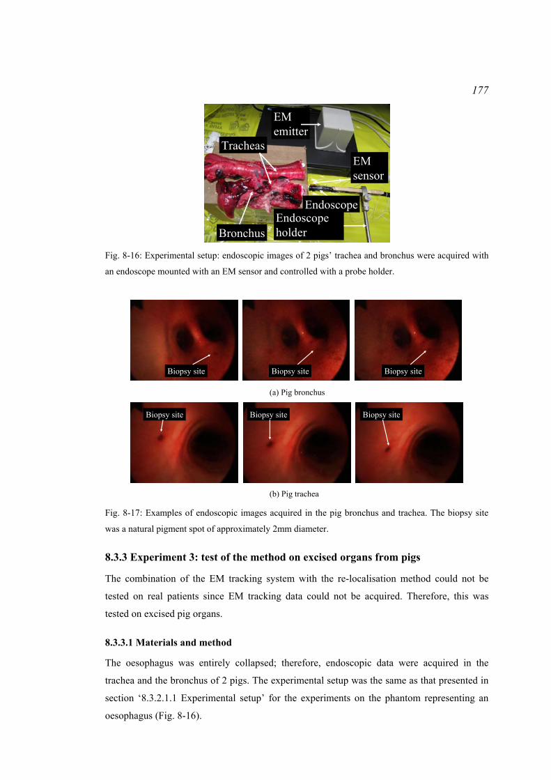
177
Tracheas
Bronchus
EMemitter
Endoscope holder
Endoscope
EM sensor
Fig. 8-16: Experimental setup: endoscopic images of 2 pigs’ trachea and bronchus were acquired with
an endoscope mounted with an EM sensor and controlled with a probe holder.
Biopsy siteBiopsy siteBiopsy site
Biopsy siteBiopsy siteBiopsy site
(a) Pig bronchus
(b) Pig trachea Fig. 8-17: Examples of endoscopic images acquired in the pig bronchus and trachea. The biopsy site
was a natural pigment spot of approximately 2mm diameter.
8.3.3 Experiment 3: test of the method on excised organs from pigs
The combination of the EM tracking system with the re-localisation method could not be
tested on real patients since EM tracking data could not be acquired. Therefore, this was
tested on excised pig organs.
8.3.3.1 Materials and method
The oesophagus was entirely collapsed; therefore, endoscopic data were acquired in the
trachea and the bronchus of 2 pigs. The experimental setup was the same as that presented in
section ‘8.3.2.1.1 Experimental setup’ for the experiments on the phantom representing an
oesophagus (Fig. 8-16).
178
The endoscope tip was moved randomly with the endoscope holder around a region
of interest to acquire a set of images in the first pig bronchus and in the second pig trachea
(Fig. 8-17). The image dimensions were 1600 pixels x 1200 pixels. For the 2 sets of images, a
target image T was selected. A pigment spot of 2mm diameter at the tissue surface was
selected as the biopsy site and its positions in the reference images Ii and in the target image
T were recorded. SIFT features were detected for each image Ii or T. As for the patient data,
a mask in the endoscopic images was used to remove the SIFT features that were detected
around the biopsy site.
The biopsy site was re-localised with 3 methods already presented in this chapter:
Method 1: Re-localisation using the EM tracking system only: For each pair of
images Ii ↔ T, the fundamental matrix ( ( )TIF ,i)EM was estimated from the EM tracking
system. Epipolar lines could be derived in T from the biopsy sites in the reference images Ii
using ( ( )TIF ,i)EM. The re-localised biopsy site could be computed in T from these epipolar
lines.
Method 2: Re-localisation without using the contribution of the EM tracking
system: For each image Ii and T, SIFT features were matched without the spatial constraint
from the EM tracking system that the matching features in T should be in a bounded region
around the epipolar line. Once the features were matched, the epipolar geometry formed by
each pair of images Ii and T was computed with the MAPSAC and the nonlinear
optimisation. Epipolar lines were derived in T from the biopsy site locations in the images Ii
to estimate the re-localised biopsy site.
Method 3: Re-localisation using the contribution of the EM tracking system:
This was the method of the whole re-localisation system presented in Chapter 8. For each pair
of images Ii ↔ T, the fundamental matrix ( ( )TIF ,i)EM was estimated from the EM tracking
system. For each image Ii and T, SIFT features were matched with the spatial constraint. A
training image was used to set the value of the width of the bounded region. The epipolar
lines were derived after refinement of the epipolar geometry with MAPSAC and a nonlinear
optimisation over the matched features. Epipolar lines were derived in T from the biopsy site
locations in the images Ii to estimate the re-localised biopsy site.
After the computation of the re-localised biopsy site, the analysis of the accuracy and
the conversion from pixels to millimetres were the same as those done for real patients in
Chapter 7. The biopsy site was re-localised with 6 epipolar lines in the pig bronchus and with
8 epipolar lines in the pig trachea. Also, for each pair of images Ii ↔ T, the number and the
percentage of inliers were counted manually.

179
a) b) c)
Without constraint:Accuracy = 30 pixels0.76mm
With constraint:Accuracy = 17 pixels0.43mm
Without constraint:Accuracy = 41 pixels1mm
With constraint:Accuracy = 12 pixels0.31mm
Fig. 8-18: Results of the experiment on excised pig bronchus and trachea: columns a) and b) re-
localisation results in bronchus and trachea: the blue epipolar lines were derived in T from the biopsy
site locations in the reference images Ii, and the green point is the re-localised biopsy site; column c)
illustration of erroneous matching (bottom) of SIFT features (top) that would be excluded by the
constraint provided by the EM tracker: a SIFT feature is represented in Ii (top row) at the centre of a
circle whose radius is proportional to the feature scale and whose drawn radius indicates the feature
orientation. The bottom row shows the matched feature in T.
8.3.3.2 Results For the ex vivo study, the spatial constraint from the EM tracking system could contribute to
more accurate re-localised biopsy sites (Fig. 8-18 a) and b)). For the sequence acquired in the
pig bronchus, one epipolar line derived from a set of matches counting 38% inliers without
spatial constraint i.e. without the contribution of the EM tracking system was less accurate
than the epipolar line derived from a set of matches counting 55% inliers with spatial
constraint (Fig. 8-18 a)). The biopsy site was re-localised with an accuracy of 1.6mm with the
EM tracking system only, 0.76mm without spatial constraint, and 0.43mm with spatial
constraint. For the sequence acquired in the trachea, one epipolar line was derived from 42
inliers without constraint while it was derived from 108 inliers with constraint (Fig. 8-18 b)).
The biopsy site was re-localised with an accuracy of 3mm with the EM tracking system only,
1mm without spatial constraint, and 0.31mm with spatial constraint. For these cases, the EM
tracking system helped avoid matching SIFT features whose neighbourhoods were similar
although they did not correspond to the same anatomical point (Fig. 8-18 c)).
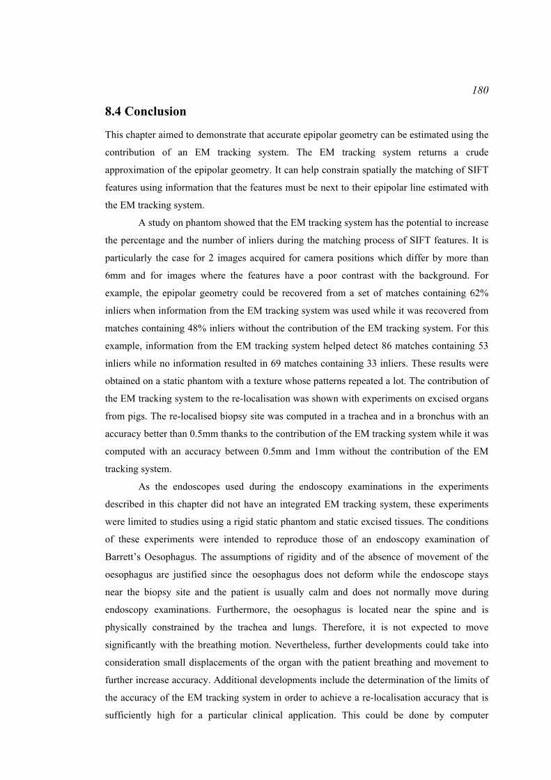
180
8.4 Conclusion
This chapter aimed to demonstrate that accurate epipolar geometry can be estimated using the
contribution of an EM tracking system. The EM tracking system returns a crude
approximation of the epipolar geometry. It can help constrain spatially the matching of SIFT
features using information that the features must be next to their epipolar line estimated with
the EM tracking system.
A study on phantom showed that the EM tracking system has the potential to increase
the percentage and the number of inliers during the matching process of SIFT features. It is
particularly the case for 2 images acquired for camera positions which differ by more than
6mm and for images where the features have a poor contrast with the background. For
example, the epipolar geometry could be recovered from a set of matches containing 62%
inliers when information from the EM tracking system was used while it was recovered from
matches containing 48% inliers without the contribution of the EM tracking system. For this
example, information from the EM tracking system helped detect 86 matches containing 53
inliers while no information resulted in 69 matches containing 33 inliers. These results were
obtained on a static phantom with a texture whose patterns repeated a lot. The contribution of
the EM tracking system to the re-localisation was shown with experiments on excised organs
from pigs. The re-localised biopsy site was computed in a trachea and in a bronchus with an
accuracy better than 0.5mm thanks to the contribution of the EM tracking system while it was
computed with an accuracy between 0.5mm and 1mm without the contribution of the EM
tracking system.
As the endoscopes used during the endoscopy examinations in the experiments
described in this chapter did not have an integrated EM tracking system, these experiments
were limited to studies using a rigid static phantom and static excised tissues. The conditions
of these experiments were intended to reproduce those of an endoscopy examination of
Barrett’s Oesophagus. The assumptions of rigidity and of the absence of movement of the
oesophagus are justified since the oesophagus does not deform while the endoscope stays
near the biopsy site and the patient is usually calm and does not normally move during
endoscopy examinations. Furthermore, the oesophagus is located near the spine and is
physically constrained by the trachea and lungs. Therefore, it is not expected to move
significantly with the breathing motion. Nevertheless, further developments could take into
consideration small displacements of the organ with the patient breathing and movement to
further increase accuracy. Additional developments include the determination of the limits of
the accuracy of the EM tracking system in order to achieve a re-localisation accuracy that is
sufficiently high for a particular clinical application. This could be done by computer
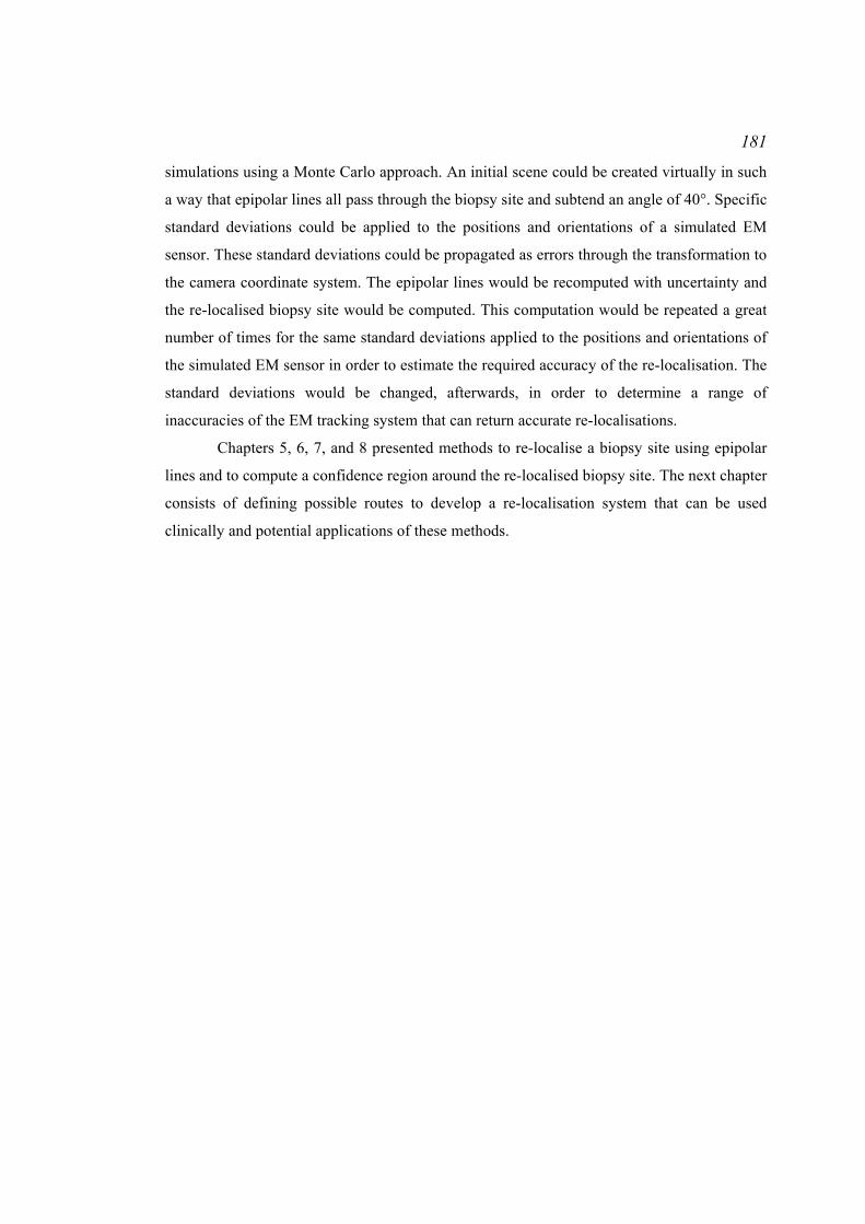
181
simulations using a Monte Carlo approach. An initial scene could be created virtually in such
a way that epipolar lines all pass through the biopsy site and subtend an angle of 40°. Specific
standard deviations could be applied to the positions and orientations of a simulated EM
sensor. These standard deviations could be propagated as errors through the transformation to
the camera coordinate system. The epipolar lines would be recomputed with uncertainty and
the re-localised biopsy site would be computed. This computation would be repeated a great
number of times for the same standard deviations applied to the positions and orientations of
the simulated EM sensor in order to estimate the required accuracy of the re-localisation. The
standard deviations would be changed, afterwards, in order to determine a range of
inaccuracies of the EM tracking system that can return accurate re-localisations.
Chapters 5, 6, 7, and 8 presented methods to re-localise a biopsy site using epipolar
lines and to compute a confidence region around the re-localised biopsy site. The next chapter
consists of defining possible routes to develop a re-localisation system that can be used
clinically and potential applications of these methods.
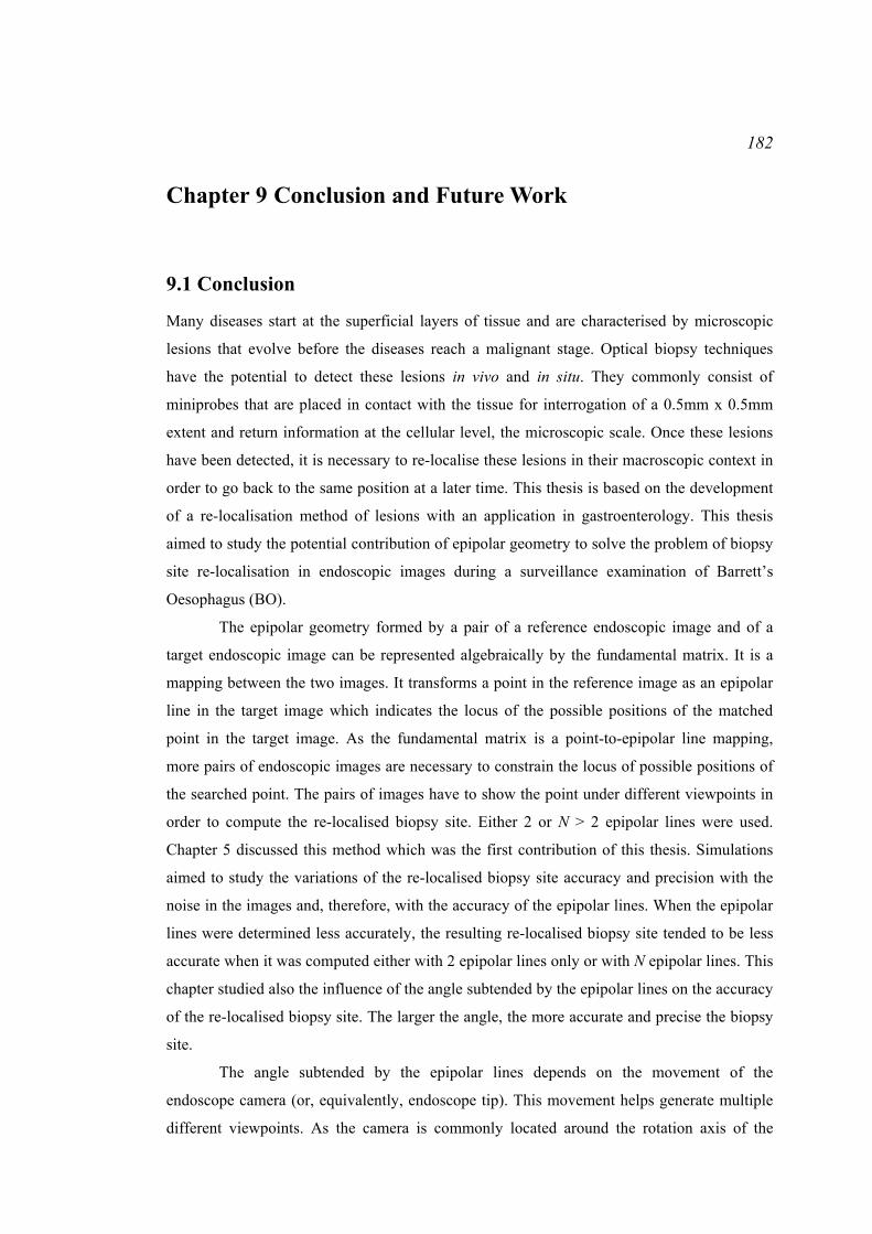
182
Chapter 9 Conclusion and Future Work
9.1 Conclusion
Many diseases start at the superficial layers of tissue and are characterised by microscopic
lesions that evolve before the diseases reach a malignant stage. Optical biopsy techniques
have the potential to detect these lesions in vivo and in situ. They commonly consist of
miniprobes that are placed in contact with the tissue for interrogation of a 0.5mm x 0.5mm
extent and return information at the cellular level, the microscopic scale. Once these lesions
have been detected, it is necessary to re-localise these lesions in their macroscopic context in
order to go back to the same position at a later time. This thesis is based on the development
of a re-localisation method of lesions with an application in gastroenterology. This thesis
aimed to study the potential contribution of epipolar geometry to solve the problem of biopsy
site re-localisation in endoscopic images during a surveillance examination of Barrett’s
Oesophagus (BO).
The epipolar geometry formed by a pair of a reference endoscopic image and of a
target endoscopic image can be represented algebraically by the fundamental matrix. It is a
mapping between the two images. It transforms a point in the reference image as an epipolar
line in the target image which indicates the locus of the possible positions of the matched
point in the target image. As the fundamental matrix is a point-to-epipolar line mapping,
more pairs of endoscopic images are necessary to constrain the locus of possible positions of
the searched point. The pairs of images have to show the point under different viewpoints in
order to compute the re-localised biopsy site. Either 2 or N > 2 epipolar lines were used.
Chapter 5 discussed this method which was the first contribution of this thesis. Simulations
aimed to study the variations of the re-localised biopsy site accuracy and precision with the
noise in the images and, therefore, with the accuracy of the epipolar lines. When the epipolar
lines were determined less accurately, the resulting re-localised biopsy site tended to be less
accurate when it was computed either with 2 epipolar lines only or with N epipolar lines. This
chapter studied also the influence of the angle subtended by the epipolar lines on the accuracy
of the re-localised biopsy site. The larger the angle, the more accurate and precise the biopsy
site.
The angle subtended by the epipolar lines depends on the movement of the
endoscope camera (or, equivalently, endoscope tip). This movement helps generate multiple
different viewpoints. As the camera is commonly located around the rotation axis of the

183
endoscope, twisting the tip of the endoscope is sufficient to translate and rotate the camera.
With such motion, the epipoles follow a circular trajectory around the centre of the image as
discussed in Chapter 7. As the biopsy site is usually not far either from the centre of the target
image, the resulting epipolar lines can subtend a large angle up to 50°. Further experiments
should be done in order to determine the minimal angle with which the endoscope tip should
be rotated for the generation of sufficiently different epipolar lines. In clinical practice, the
epipolar lines could also be overlaid on the images in order to help the endoscopist decide
how to rotate the endoscope.
During an endoscopic examination, the display of a confidence region around the re-
localised biopsy site may be useful for instrument guidance. The confidence region of a point
is commonly drawn from the covariance matrix of this point. The covariance matrix can be
determined experimentally which consists of estimating the point several times adding
different noise samples in the images for each experiment. This method requires, however, a
lot of iterations. Chapter 6 presented an analytical derivation for the determination of this
covariance matrix without iterations which was the second contribution of this thesis. The
derivation was developed for the re-localisation method with N > 2 epipolar lines. The
resulting analytical covariance matrices were not in perfect correspondence with the
experimental covariance matrices. However, these derivations have the potential to display an
approximation of the confidence region around the re-localised biopsy site.
Chapter 5 and Chapter 6 focused on the use of epipolar lines to re-localise a biopsy
site and on analytical derivations to estimate the confidence region around the site in the
target image. Chapter 7 presented the results of the validation of the re-localisation method
and of the analytical uncertainty. The validation was done using data acquired on a phantom
and on real patients with various endoscopes and various endoscope camera motions. During
some examinations, air/water bubbles obstruct the field of view of the endoscope camera or
the camera may move too quickly which returns blurred images. These events may happen
between the time before which the endoscopist was interrogating the tissue with the
miniprobe and the time after which the biopsy site needed to be re-localised. The recovery of
the epipolar geometry between the reference image and the target image requires the
detection of common features which are commonly located on the vasculature. When events
like air/water bubbles appearance or quick camera movement does not occur, the Lucas
Kanade (LK) tracker may be used to detect features in the reference image and to track them
until the target image. This tracker has the advantage of constraining spatially the search for
the feature matches. However, in the case of such events, the LK tracker fails since features
cannot be tracked reliably. The Scale and Invariant Feature Transform (SIFT) may be used as
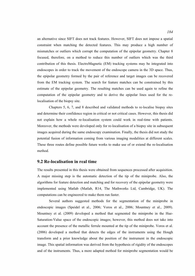
184
an alternative since SIFT does not track features. However, SIFT does not impose a spatial
constraint when matching the detected features. This may produce a high number of
mismatches or outliers which corrupt the computation of the epipolar geometry. Chapter 8
focused, therefore, on a method to reduce this number of outliers which was the third
contribution of this thesis. ElectroMagnetic (EM) tracking systems may be integrated into
endoscopes in order to track the movement of the endoscope camera in the 3D space. Thus,
the epipolar geometry formed by the pair of reference and target images can be recovered
from the EM tracking system. The search for feature matches can be constrained by this
estimate of the epipolar geometry. The resulting matches can be used again to refine the
computation of the epipolar geometry and to derive the epipolar lines used for the re-
localisation of the biopsy site.
Chapters 5, 6, 7, and 8 described and validated methods to re-localise biopsy sites
and determine their confidence region in critical or not critical cases. However, this thesis did
not explain how a whole re-localisation system could work in real-time with patients.
Moreover, the methods were developed only for re-localisation of a biopsy site in subsequent
images acquired during the same endoscopy examination. Finally, the thesis did not study the
potential fusion of information coming from various imaging modalities at different scales.
These three routes define possible future works to make use of or extend the re-localisation
method.
9.2 Re-localisation in real time
The results presented in this thesis were obtained from sequences processed after acquisition.
A major missing step is the automatic detection of the tip of the miniprobe. Also, the
algorithms for feature detection and matching and for recovery of the epipolar geometry were
implemented using Matlab (Matlab, R14, The Mathworks Ltd, Cambridge, UK). The
computations can be engineered to make them run faster.
Several authors suggested methods for the segmentation of the miniprobe in
endoscopic images (Speidel et al., 2006; Voros et al., 2006; Mountney et al., 2009).
Mountney et al. (2009) developed a method that segmented the miniprobe in the Hue-
Saturation-Value space of the endoscopic images; however, this method does not take into
account the presence of the metallic ferrule mounted at the tip of the miniprobe. Voros et al.
(2006) developed a method that detects the edges of the instruments using the Hough
transform and a prior knowledge about the position of the instrument in the endoscopic
image. This spatial information was derived from the hypothesis of rigidity of the endoscopes
and of the instruments. Thus, a more adapted method for miniprobe segmentation would be

185
that developed by Speidel et al. (2006) which is probabilistic segmentation using information
about the colour of the pixels to distinguish tissue from the instruments.
Implementations of the Lucas Kanade (LK) tracker and of the Scale Invariant Feature
Transform (SIFT) used in this thesis were not fast implementations. Graphic Processing Unit
(GPU) implementations of these algorithms have been developed and can be found at the
following adresses:
- GPU-based LK tracker: http://www.cs.unc.edu/~ssinha/Research/GPU_KLT/
- GPU-based SIFT: http://www.cs.unc.edu/~ccwu/siftgpu/
Furthermore, the estimation of the fundamental matrices requires a lot of MAPSAC tests .
These tests can be run in parallel using the GPU technology. In this thesis, a 7-parameter non-
linear optimisation method based on MAPSAC was used for the estimation of the
fundamental matrix. A recently desribed alternative method termed the Extended
Fundamental Numerical Scheme (EFNS), developed by Sugaya and Kanatani (Sugaya and
Kanatani, 2007; Kanatani, 2008), has been shown to return a more accurate fundamental
matrix than that obtained with the 7-parameter non-linear optimisation. The EFNS method
consists of minimising the uncertainty of the fundamental matrix represented by its
covariance matrix. Future developments could explore this method in order to improve the re-
localisation accuracy.
Finally, the method presented in this thesis made the assumption that the oesophagus
tissue does not deform significantly. Most of the patients undergoing the endoscopy
examinations for the surveillance of Barrett’s Oesophagus whose data were acquired for the
validation studies presented in this thesis were sedated and calm during the examination.
Therefore, the oesophageal wall could be reasonably assumed to remain stationary during the
examination once the endoscope had been inserted. Furthermore, the processed sequences
were selected such that they showed a static structure of the oesophagus. For some patients,
the oesophageal wall was observed to exhibit a periodical movement when the miniprobe was
removed: the wall shrunk and distended again as the oesophagus recovered its initial shape.
Future work could focus on the detection of endoscope images during a sequence which
shows the same oesophagus shape. One possible approach would be to recover the epipolar
geometry and to measure the Sampson’s error for the fundamental matrix to fit the set of
inliers. If the Sampson’s error is too large, this indicates that the reference image might not be
suitable for use in re-localisation.
These three improvements will be investigated in future developments.
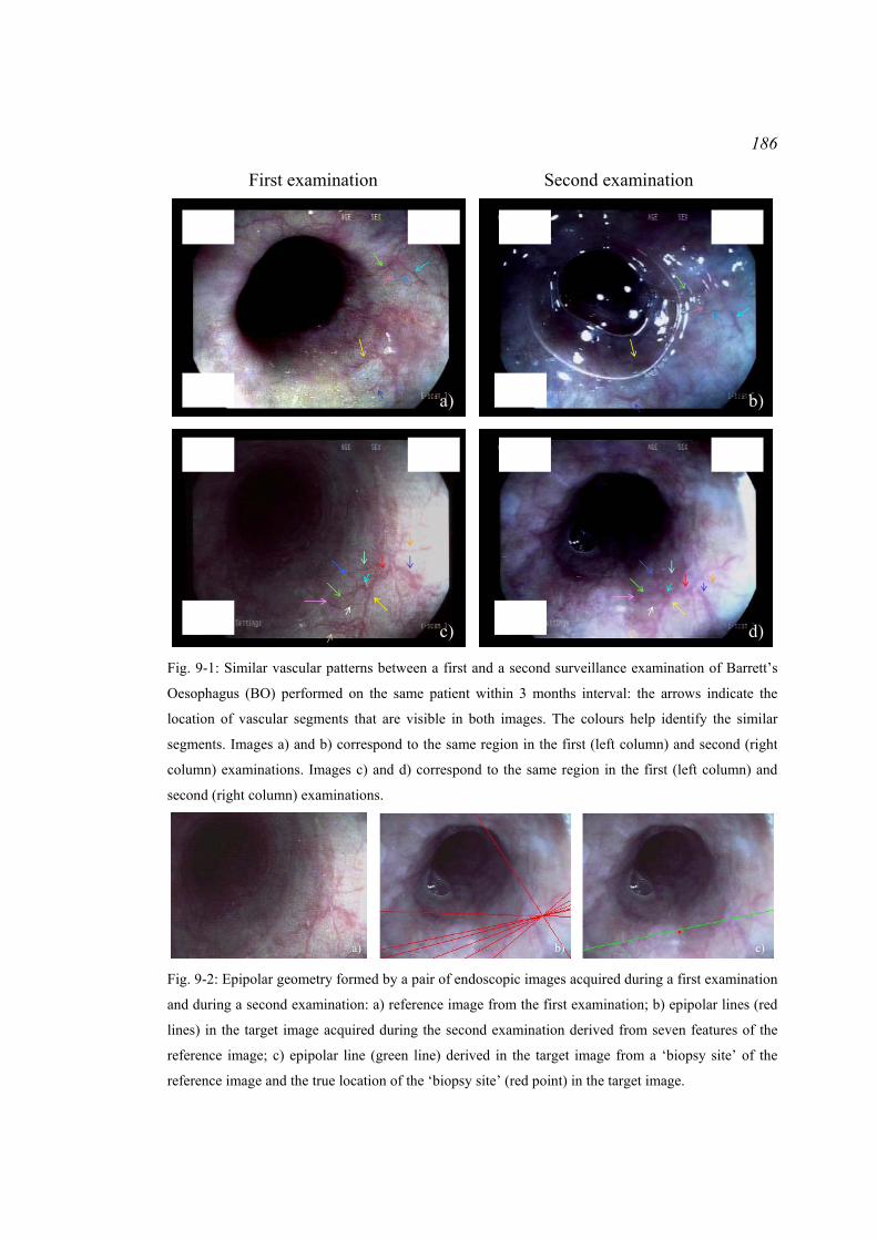
186
First examination Second examination
a) b)
c) d)
Fig. 9-1: Similar vascular patterns between a first and a second surveillance examination of Barrett’s
Oesophagus (BO) performed on the same patient within 3 months interval: the arrows indicate the
location of vascular segments that are visible in both images. The colours help identify the similar
segments. Images a) and b) correspond to the same region in the first (left column) and second (right
column) examinations. Images c) and d) correspond to the same region in the first (left column) and
second (right column) examinations.
b) c)a) Fig. 9-2: Epipolar geometry formed by a pair of endoscopic images acquired during a first examination
and during a second examination: a) reference image from the first examination; b) epipolar lines (red
lines) in the target image acquired during the second examination derived from seven features of the
reference image; c) epipolar line (green line) derived in the target image from a ‘biopsy site’ of the
reference image and the true location of the ‘biopsy site’ (red point) in the target image.
187
9.3 Biopsy site re-localisation in a future examination
A surveillance examination of Barrett’s Oesophagus (BO) consists of detecting dysplasias at
the tissue surface that correspond to early changes of the cells. These cells can evolve over
time as cancers or they can get back to normal. An important extension of the re-localisation
method would be its use for excising or observing during a future examination the biopsy site
detected in a first examination in order to assess the stage of the disease.
The re-localisation method requires the detection of features in endoscopic images
that correspond usually to vessel intersections or curvatures. As patients examined for the
detection of BO do not have cancer, it is not expected that the geometry and/or size of
superficial blood vessels will change significantly between endoscopic investigations due to
the angiogenesis. Therefore, it is reasonable to assume that there will not be significant
changes in the appearance of the wall of the oesophagus. An experiment consisted of
comparing the oesophagus wall of the same patient observed with an endoscope during two
surveillance examinations within 3 months interval. Given an image from the second
examination, corresponding images from the first examination were searched by
identification of similar vasculature. Once corresponding images were found, SIFT features
were detected and matched. A point was selected as the biopsy site in the images. The
epipolar geometry was recovered using seven pairs of good matches for a pair of images from
respectively the first examination and the second examination. The epipolar line
corresponding to the biopsy site was derived in the image of the second examination termed
target image.
This experiment showed that similarities in the oesophagus walls could be found
between 2 examinations (Fig. 9-1). Because of the difference of the endoscope optics, of the
camera orientations, and of the image resolutions, only a small section of the images showed
similarities and most of the common features were concentrated in this small section. Thus,
the epipolar geometries and the re-localised biopsy site risk being less accurate than those
computed during the same examination. Nevertheless, the computation of the epipolar
geometry formed by the pair of images shown in Fig. 9-2 returned an accurate epipolar line
for the re-localisation of the biopsy site. This accuracy was maybe due to the selection of
good feature matches for the recovery of the epipolar geometry.
A possible approach for biopsy site re-localisation during a future examination would
be, first, the selection of the reference endoscopic images from the first examination that
show the same part of the oesophagus as the current target image from the second
examination. Mori et al. (2005) demonstrated that an ElectroMagnetic (EM) tracking system
returns information about the location of the endoscope camera in the organ of interest and

188
has the potential to reduce the computations by selection of images that are spatially relevant
during the same examination. Future work for biopsy site re-localisation will focus on the
potential use of an EM tracking system to reposition roughly the endoscope around the
biopsy site that was detected during a previous examination. Secondly, the detected SIFT
features could be matched using a graph matching method presented by Atasoy et al. (2009)
which took into account the visual similarity of the features and which preserved their spatial
arrangement in order to increase the proportion of the inliers. The strong constraint from the
EM tracking system can also be integrated into this method to reduce the complexity of the
graph matching. Finally, high resolution images will be acquired in order to improve the
feature detection and matching.
9.4 Biopsy site re-localisation in lungs and fusion of imaging
modalities
a)
b)
c) d)
e) f)
Fig. 9-3: Characterisation of a tumour with various imaging modalities: a) normal cell arrangements at
the surface of the lung walls observed with in vivo fibered confocal microscopy are differentiated from
b) abnormal arrangements for which the cells look disorganised; c) tumours can also be detected in the
pre-operative CT image and under a guidance of the bronchoscope, the endoscopist can perform d)
endobronchoscopic ultra sound imaging in order to detect the tumour in vivo and e) to excise tissue for
observation under a microscope; f) the tumour can also be observed with optical coherence
tomography.
Image not displayed for Copyright reasons
189
Cancers in organs different from the oesophagus are also preceded by cell changes that can be
detected in vivo by optical biopsy at an early stage. For example, the early detection of
recurrent respiratory papillomatosis helps avoid the development of cancers in lung (Colt et
al., 2010). Information about the cell structures in lung can come from a variety of imaging
modalities such as a pre-operative CT image, EndoBronchoscopic Ultra Sound (EBUS)
images, Optical Coherence Tomography (OCT) images, or Fibered Confocal Microscopy
(FCM) images (Fig. 9-3). An important issue is the coregistration of these different sources of
information.
The pre-operative CT image helps identify the tumours in the organ (Fig. 9-3 c)).
During the endoscopic examination, a navigation system can be used to guide the
bronchoscope towards the tumour locations (Mori et al., 2005, 2006, 2007, 2008, 2009;
Valdivia, 2010). This navigation system registers the real bronchoscope camera movement in
a 3D reconstruction of the lungs from the pre-operative CT image. Once the bronchoscope is
placed around the tumour, imaging or surgical instruments such as EBUS, FCM, or OCT
probes can be used to analyse the tissue surface under the visual control of the bronchoscope
camera. They return information about the tissue structure (Fig. 9-3 a), b), d), f)).
Chapter 8 showed that the re-localisation method in combination with an EM
tracking system can be used as well in the trachea or in the bronchus. Therefore, the sites
analysed with EBUS, FCM, and OCT probes can be re-localised in the bronchoscopic image
for guidance of biopsy needles for excision and for ex vivo analysis under a microscope (Fig.
9-3 e)) in order to confirm the diagnosis made with the pre-operative image and in vivo. An
EM sensor could be mounted at the tip of the endoscope and could be used to localise the
endoscope pose both in physical space and, through registration, in the pre-operative CT
image. The ultrasound probe is usually mounted onto to the endoscope tip for EBUS
applications. Thus, there is a rigid transformation from the coordinate system of the
ultrasound probe to the endoscope camera coordinate system. As the optical miniprobes for
FCM or OCT are passed through the working channel of the endoscope and are visible in the
endoscope images, the tip of the miniprobe can be localised in the endoscope images and,
again by transforming between coordinates, in the pre-operative image.
Future development can focus on the integration of the re-localisation method in a
clinical system for image-guided biopsy within the airways.
190
9.5 Integration of the re-localisation method in a Magnetic
Resonance-guided system
An application of the re-localisation method is the guidance of instruments or cells for
treatment of the tissue extent affected by malignancies. Riegler et al. (2011) demonstrated
that magnetic and fluorescent cells can be steered to a site of interest using the magnetic force
derived from the coils of a Magnetic Resonance (MR) scanner. These cells were fluorescent
in order to be visible in in vivo Fibered Confocal Microscopy (FCM) images. Therefore, the
cell movement could be controlled using an FCM miniprobe.
This method could be integrated into an interventional system combining endoscopy,
optical biopsy such as FCM, and MR imaging for biopsy site re-localisation and treatment.
MR imaging has been shown to be an appropriate tool for the detection of cancers in the
oesophagus (Ajaj et al., 2004; Iwadate et al., 2007). As MR imaging has the potential to
guide interventions (Kos et al., 2007), MR images could be acquired during endoscopic
examinations in the oesophagus in order to track visually the position of the optical biopsy
miniprobe within the organ. If the endoscope were MR-compatible as one was presented in
Gross et al. (2001), the endoscopy could be performed under the control of the MR scanner.
Once the biopsy site has been detected in the endoscopic images, the re-localisation method
in the endoscopic images could help maintain the optical biopsy miniprobe at the location of
the biopsy site. The MR scanner would be used to guide the cells for tissue treatment towards
the detected site as described in Riegler et al. (2011).
The tracking of the FCM miniprobe tip may be useful to record the location of the
treated site as presented in Chapter 2 ‘Initial Pilot Work to Assess the In Vivo Use of the
Fibered Confocal Microscope and its Use in Combination with MRI’. Because the
oesophagus is full of air, it will appear in black in the MR images. In this case, a Gadolinium-
based marker can be mounted at the tip of the FCM miniprobe in order to make it visible as
presented in Chapter 2. The positions of the FCM miniprobe can be, therefore, recorded in
the MR images with the method described in Chapter 2. This position can be finally used to
steer the cells to the site to be treated using the forces derived from the MR imaging coils.

191
Publications First Author:
Allain, B., Hu, M., Lovat, L.B., Cook, R.J., Ourselin, S., and Hawkes, D.J., 2009a, Biopsy
Site Re-localisation based on the Computation of Epipolar Lines from Two Previous
Endoscopic Images, In: G.Z. Yang, D.J. Hawkes, D. Rueckert (eds.) MICCAI 2009, LNCS,
Part I, volume 5761, pages 491-498, Springer, Heidelberg.
Allain, B., Price, A., Vercauteren, T.K., Cook, R.J., Ourselin, S., Lythgoe, M.F., and Hawkes,
D.J., 2009b, Precision of Confocal Miniprobe Localisation Assessed By High-Field Magnetic
Resonance Imaging, Gastrointestinal endoscopy, volume 69, issue 5, page AB370.
Allain, B., Hu, M., Lovat, L.B., Cook, R.J., Vercauteren, T., Ourselin, S., and Hawkes, D.J.,
2010, A System for Biopsy Site Re-targeting with Uncertainty in Gastroenterology and
Oropharyngeal Examinations, In: T. Jiang, N. Navab, J.P.W. Pluim, M.A. Viergevier (eds.)
MICCAI 2010, LNCS, Part II, volume 6362, pages 514-521, Springer, Heidelberg.
Allain, B., Hu, M., Lovat, L.B., Cook, R.J., Vercauteren, T., Ourselin, S., and Hawkes, D.J.,
2011, Re-localisation of a Biopsy Site in Endoscopic Images and Characterisation of its
Uncertainty, Medical Image Analysis (2011), In Press, DOI 10.1016/j.media.2011.11.005.
Second Author:
Hu, M., Allain, B., Hawkes, D., Ourselin, S., Lovat, L., Cook, R., 2009, Apparatus and
Method for Determining a Location in a Target Image, WO/2011/027107,
PCT/GB2010/001651.
Riegler, J., Allain, B., Cook, R. J., Lythgoe, M. F., and Pankhurst, Q. A., 2011, Magnetically
Assisted Delivery of Cells Using Magnetic Resonance Imaging System, Journal of Physics
D: Applied Physics, volume 44, number 5, 055001.

192
Bibliography Abrat, B., and Masters, A., 2006, Endoscopic Confocal Microscopy Moves into the Clinic,
Biophotonics international, Laurin.
Ajaj, W., Debatin, J.F., and Lauenstein, T., 2004, Dark Lumen MR Colonography,
Abdominal Imaging, volume 29, number 4, pages 429-433.
Al-Gubory, K.H., and Houdebine, L.M., 2006, In Vivo Imaging of Green Fluorescent Protein-
expressing Cells in Transgenic Animals using Fibred Confocal Fluorescence Microscopy,
European Journal of Cell Biology, volume 85, pages 837-845.
Allain, B., Hu, M., Lovat, L.B., Cook, R.J., Ourselin, S., and Hawkes, D.J., 2009a, Biopsy
Site Re-localisation based on the Computation of Epipolar Lines from Two Previous
Endoscopic Images, In: G.Z. Yang, D.J. Hawkes, D. Rueckert (eds.) MICCAI 2009, LNCS,
Part I, volume 5761, pages 491-498, Springer, Heidelberg.
Allain, B., Price, A., Vercauteren, T.K., Cook, R.J., Ourselin, S., Lythgoe, M.F., and Hawkes,
D.J., 2009b, Precision of Confocal Miniprobe Localisation Assessed By High-Field Magnetic
Resonance Imaging, Gastrointestinal endoscopy, volume 69, issue 5, page AB370.
Allain, B., Hu, M., Lovat, L.B., Cook, R.J., Vercauteren, T., Ourselin, S., and Hawkes, D.J.,
2010, A System for Biopsy Site Re-targeting with Uncertainty in Gastroenterology and
Oropharyngeal Examinations, In: T. Jiang, N. Navab, J.P.W. Pluim, M.A. Viergevier (eds.)
MICCAI 2010, LNCS, Part II, volume 6362, pages 514-521, Springer, Heidelberg.
Anderson, T., 1958, An Introduction to Multivariate Statistical Analysis, John Wiley & Sons,
Inc.
Atasoy, S., Glocker, B., Giannarou, S., Mateus, D., Meining, A., Yang, G.Z., and Navab, N.,
2009, Probabilistic Region Matching in Narrow-Band Endoscopy for Targeted Optical
Biopsy, In: G.A. Yang, D.J. Hawkes, D. Rueckert (eds.) MICCAI 2009, LNCS, Part I,
volume 5761, pages 499-506, Springer, Heidelberg.

193
Bartels, L.W., and Bakker, C.J.G., 2003, Endovascular Interventional Magnetic Resonance
Imaging, Physics in Medicine and Biology, volume 48, pages R37-R64.
Barreto, J.P., and Daniilidis, K., 2005, Fundamental Matrix for Cameras with Radial
Distortion, ICCV 2005, volume 1, pages 625-632.
Becker, V., Vercauteren, T., Hann von Weyhern, C., Prinz, C., Schmid, R.M., and Meining,
A., 2007, High-Resolution Miniprobe-Based Confocal Microscopy in Combination with
Video Mosaicing, Gastrointestinal Endoscopy, volume 66, number 5, pages 1001-1007.
Bjorck, A., 1996, Numerical Methods for Least Squares Problems, Philadelphia, SIAM.
Boggs, P.T., and Wolle, J.W., 1996, Sequential Quadratic Programming, Acta Numerica,
volume 4, number 1, pages 1-51.
Bookstein, F., 1979, Fitting Conic Sections to Scattered Data, Computer Vision Graphics and
Image Processing, volume 9, pages 56-71.
Botoman, V.A., Pietro, M., and Thirlby, R.C., 1994, Localization of Colonic Lesions with
Endoscopic Tattoo, Journal of Diseases of the Colon and Rectum, volume 37, number 8,
pages 775-776.
Bouguet, J.Y., 2004, Camera Calibration Toolbox for Matlab.
http://www.vision.caltech.edu/bouguetj/calib_doc.
British Society of Gastroenterology, 2005, Guidelines for the Diagnosis and Management of
Barrett’s Columnar-Lined Oesophagus, http://www.bsg.org.uk.
Brown, M., and Lowe, D.G, 2006, Automatic Panoramic Image Stitching using Invariant
Features, International Journal of Computer Vision, volume 74, number 1, pages 59-73.
Burstin, von, J., Eser, S., Seidler, B., Meining A., Bajbouj, M., Mages, J., Lang, R., Kind,
A.J., Schnieke, A.E., Schmid, R.M., Schneider, G., and Saur, D., 2008, Highly Sensitive
Detection of Early-Stage Pancreatice Cancer by Multimodal Near-Infrared Molecular
Imaging in Living Mice, International Journal of Cancer, volume 123, pages 2138-2147.

194
Burschka, D., Li, M., Ishii, M., Taylor, R.H., and Hager, G.D., 2005, Scale-Invariant
Registration of Monocular Endoscopic Images to CT-Scans for Sinus Surgery, Medical
Image Analysis, volume 9, Issue 5, pages 413-426.
Cardoso, J.F., 1997, Infomax and Maximum Liklihood for Blind Source Separation, IEEE
Signal Processing Letters, volume 4, number 4, pages 112-114.
Colt, H.G., Murgu, S.D., Jung, B., Ahn, Y.C., and Brenner, M., 2010, Multimodality
Bronchoscopic Imaging of Recurrent Respiratory Papillomatosis, The Laryngoscope, volume
120, issue 3, pages 468-472.
Cotton, P., and Williams, C., 1996, Practical Gastrointestinal Endoscopy, Blackwell
Scientific, London.
Csurka, G., Zeller, C., Zhang, Z., and Faugeras, O.D., 1997, Characterising the Uncertainty
of the Fundamental Matrix, Computer Vision and Image Understanding, volume 68, number
1, pages 18-36.
Dahr, A., Kristie, S.J., Novelli, M.R., Bown, S.G., Bigio, I.J., Lovat, L.B., and Bloom, S.L.,
2006, Elastic Scattering Spectroscopy for the Diagnosis of Colonic Lesions: Initial Results of
a Novel Optical Biopsy Technique. In: Gastrointestinal Endoscopy, volume 63, issue 2, pages
257-261.
Davison, A.J., Reid, I.D., Molton, N.D., and Stasse, O., 2007, MonoSLAM: Real-Time
Single Camera SLAM, IEEE Transactions On Pattern Analysis And Machine Intelligence,
volume 29, number 6, pages 1052-1067.
Deguchi, D., Mori, K., Suenaga, Y., Hasegawa, J.I., Toriwaki, J.I., Natori, H., and
Takabatake, H., 2003, New Calculation Method of Image Similarity for Endoscope Tracking
Based on Image Registration in Endoscope Navigation, Computer Assisted Radiology and
Surgery, Proceedings of the 17th International Congress and Exhibition, volume 1256, pages
460-466.
Deguchi, D., Mori, K., Suenaga, Y., Hasegawa, J.I., Toriwaki, J.I., Takabatake, H., and
Natori, H., 2007, New Image Similarity Measure for Bronchoscope Tracking Based on Image
195
Registration. In: R.E. Ellis, and T.M. Peters (eds.) MICCAI 2003, LNCS, volume 2878,
pages 399-406, Springer, Heidelberg.
Denk, W., Piston, D.W., Webb, W.W., and Pawley, J.B., 1995, Handbook of Biological
Confocal Microscopy, Plenum Press, New York.
Deriche, R., Zhang, Z., Luong, Q.T., and Faugeras, O.D., 1994, Robust Recovery of the
Epipolar Geometry for an Uncalibrated Stereo Rig, ECCV 1994, volume 1, LNCS, volume
800, Springer-Verlag, pages 567-576.
Dey, D., Gobbi, D.G., Slomka, P.J., Surry, K.J.M., and Peters, T.M., 2002, Automatic Fusion
of Freehand Endoscopic Brain Images to Three-Dimensional Surfaces: Creating Stereoscopic
Panoramas, IEEE Transactions on Medical Imaging, volume 21, number 1, pages 23-30.
Eguchi, S., and Copas, J., 2006, Interpreting Kullback-Leibler Divergence with the Neyman-
Pearson Lemma, Journal of Multivariate Analysis, volume 97, pages 2034-2040.
Evans, J.A., Poneros, J.M., Bouma, B.E., Bressner, J., Halpern, E.F., Shishkov, M., Lauwers,
G.Y., Mino-Kenudson, M., Nishioka, N.S., and Tearney, G.J., 2006, Optical Coherence
Tomography to Identify Intramucosal Carcinoma and High-Grade Dysplasia in Barrett’s
Esophagus, Journal of Clinical Gastroenterology and Hepatology, volume 4, issue 1, pages
38-43.
Faugeras, O.D., 1993, Three-Dimensional Computer Vision: a Geometric Viewpoint, MIT
Press, Cambridge, MA/London.
Faugeras, O., and Robert, L., 1994, What Can Two Images Tell Us About a Third One?,
ECCV 1994, LNCS, volume 800, pages 485-492.
Fujimoto, J., 2003, Optical Coherence Tomography for Ultrahigh Resolution In Vivo
Imaging, Nature Biotechnology, volume 21, pages 1361-1367.
Fischler M.A. and Bolles R.C., 1981, Random Sample Consensus: a Paradigm for Model
Fitting with Applications to Image Analysis and Automated Cartography, Communications
of the ACM, volume 24, number 6, pages 381-395.
196
Gross, P., Kitney, R.I., Claesen, S., and Halls, J.M., 2001, MR-Compatible Endoscopy and
Tracking for Image-Guided Surgery, Computer Assisted Radiology and Surgery, volume
1230, pages 1076-1082.
Haneishi, H., Yagihashi, Y., and Miyake, Y., 1995, A New Method for Distortion Correction
of Electronic Endoscope Images, IEEE Transactions on Medical Imaging, volume 14, pages
548-55.
Hartley, R.I., 1995, In Defence of the 8-Point Algorithm, ICCV 1995, pages 1064-1070.
Hartley, R.I., 1997, Triangulation, Computer Vision and Image Understanding, volume 68,
number 2, pages 146-157.
Hartley, R.I., and Zisserman, A., 2004, Multiple View Geometry in Computer Vision.
Cambridge University Press, Cambridge.
Helferty, J.P., Zhang, C., McLennan, G., and Higgins, W. E., 2001, Videoendoscopic
Distortion Correction and its Application to Virtual Guidance of Endoscopy, IEEE
Transactions on Medical Imaging, volume 20, pages 605-617.
Helferty, J.P. and Higgins, W.E., 2002, Combined Endoscopic Video Tracking and Virtual
3D CT Registration for Surgical Guidance, ICCV 2002, volume 2, pages II-961-II-964.
Helferty, J.P., Sherbondy, A.J., Kiraly, A.P., and Higgins, W.E., 2007, Computer-Based
System for the Virtual-Endoscopic Guidance of Bronchoscopy, Computer Vision and Image
Understanding, volume 108, issues 1-2, pages 171-187.
Hsiung, P.L., Hardy, J., Friedland, S., Soetikno, R., Du, C.B, Wu, A.P., Sahbaie, P.,
Crawford, J.M., Lowe, A.W., Contag, C.H., and Wang, T.D., 2008, Detection of Colonic
Dysplasia In Vivo Using a Targeted Heptapeptide and Confocal Microendoscopy, Nature
Medicine, volume 14, number 4, pages 454-458.
Hu, M., Penney, G., Edwards, P., Figl, M., and Hawkes, D.J., 2007, 3D Reconstruction of
Internal Organ Surfaces for Minimal Invasive Surgery. In: N. Ayache, S. Ourselin, A.
Maeder (eds.) MICCAI 2007, Part I LNCS, volume 4791, pages 68-77, Springer, Heidelberg.

197
Hu, M., Penney, G., Rueckert, D., Edwards, P., Figl, M., Pratt, P., and Hawkes, D.J., 2008a,
A novel Algorithm for Heart Motion Analysis Based on Geometric Constraints, In: D.
Metaxas, L. Axel, G. Fichtinger, G. Szekely (eds.) MICCAI 2008, part I. LNCS, volume
5241, pages 720-728, Springer-Verlag.
Hu, M., McMenemy, K., Ferguson, S., Dodds, G., Yuan, B., 2008b, Epipolar Geometry
Estimation Based on Evolutionary Agents, Pattern Recognition, volume 41, issue 2, pages
575-591.
Hu, M., Penney, G.P., Rueckert, D., Edwards, P.J., Bello, F., Casula, R., Figl, M., and
Hawkes, D.J., 2009, Non-Rigid Reconstruction of the Beating Heart Surface for Minimally
Invasive Cardiac Surgery. In: G.Z. Yang, D.J. Hawkes, D. Rueckert (eds.) MICCAI 2009,
Part I, LNCS, volume 5761, pages 34-42. Springer, Heidelberg.
Hummel, J.B., Bax, M.R., Figl, M.L., Kang, Y., Maurer, Jr., C., Birkfellner, W.W.,
Bergmann, H., and Shahidi, R., 2005, Design and Application of an Assessment Protocol for
Electromagnetic Tracking System, Medical Physics, volume 32, issue 7, pages 2371-2379.
ISO 5725-1, 1994, Accuracy (Trueness and Precision) of Measurement Methods and Results
– Part 1: General principles and definitions.
Iwadate, Y., Goto, T., Nabetani, A., Miyoshi, M., Asano, K., and Tsukamoto, T., 2007,
Esophagus Imaging by 3D FSE with Combination of Inner Volume Excitation and Variable
Refocusing Flip Angles, In Proceedings of the International Society for Magnetic Resonance
in Medicine, page 2729.
Johnson, R.A., and Wichern, D.W., 1998, Applied Multivariate Statistical Analysis, Prentice-
Hall, Upper Saddle River.
Kanatani, K., 2008, Statistical Optimization for Geometric Fitting: Theoretical Accuracy
Bound and High Order Error Analysis, International Journal of Computer Vision, volume 80,
pages 167-188.
Katzir, A., 1993, Lasers and Optical Fibers in Medicine, Academic Press Incorporation.
198
Kendall, M., and Stuart, A., 1983, The Advanced Theory of Statistics, Charles Griffin and
Company: London.
Koenderink, J.J., 1984, The Structure of Images, Biological Cybernetics, volume 50, pages
363-370.
Kos, S., Huegli, R., Bongartz, G.M., Jacob, A.L., and Bilecen D., 2007, MR-Guided
Endovascular Interventions: a Comprehensive Review on Techniques and Applications,
European Society of Radiology, volume 18, number 4, pages 645-657.
Krupa, A., Gangloff, J., Doignon, C., de Mathelin, M.F., Morel, G., Leroy, J., Soler, L., and
Marescaux, J., 2003, Autonomous 3-D Positioning of Surgical Instruments in Robotized
Laparoscopic Surgery using Visual Servoing, IEEE Transactions on Robotics and
Automation, volume 19, pages 842-853.
Kuhn H.W., 1976, Nonlinear Programming: A Historical View, SIAM-AMS Proceedings,
volume 9, pages 1-26.
Kullback, S., 1959, Information Theory and Statistics, John Wiley and Sons, NY.
Le Goualher, G., Perchant, A., Genet, M., Cavé, C., Viellerobe, B., Bérier, F., Abrat, B., and
Ayache, N., 2004, Towards Optical Biopsies with an integrated Fibered Confocal
Fluorescence Microscope, In: C. Barillot, D.R. Haynor, P. Hellier (eds.) MICCAI 2004,
volume 3217, LNCS, pages 761-768, Springer-Verlag.
Lindeberg, T., 1994, Scale-Space Theory: A Basic Tool for Analysing Structures at Different
Scales, Journal of Applied Statistics, volume 21, number 2, pages 224-270.
Lindeberg, T., and Garding, J., 1997, Shape-Adapted Smoothing in Estimation of 3-D Shape
Cues from Affine Deformations of Local 2-D Brightness Structure, Image and Vision
Computing, volume 15, number 6, pages 415-434.
Lindeberg, T., 1998, Feature Detection with Automatic Scale Selection, International Journal
of Computer Vision, volume 30, number 2, pages 79-116.

199
Longuet-Higgins, H.C., 1981, A Computer Algorithm for Reconstructing a Scene from Two
Projections, Nature, 293, pages 133-135.
Lovat, L.B., and Bown, S.G., 2004, Elastic Scattering Spectroscopy for Detection of
Dysplasia in Barrett’s Esophagus, In: Gastrointestinal Endoscopy Clinics of North America:
optical biopsy, Amsterdam: Elsevier, volume 14, issue 3, pages 507-517.
Lovat, L.B., Johnson, K., Mackenzie, G.D., Clark B.R., Novelli, M.R., Davies, S.,
O’Donovan, M., Selvasekar, C., Thorpe, S.M., Pickard, D., Fitzgerald, R., Fearn, T., Bigio,
I., and Bown, S.G., 2006, Elastic Scattering Spectroscopy Accurately Detects High Grade
Dysplasia and Cancer in Barrett's oesophagus, Gut 55, pages 1078-1083.
Lowe, D.G., 2004, Distinctive Image Features from Scale-Invariant Keypoints, International
Journal of Computer Vision, volume 60, number 2, pages 91-110.
Lucas, B., and Kanade, T., 1981, An Iterative Image Registration Technique with an
Application to Stereo Vision, in Proceedings of IJCAI, pages 674-679.
Luo, X., Feuerstein, M., Reichl, T., Kitasaka, T., and Mori, K., 2010, An Application Driven
Comparison of Sevral Feature Extraction Algorithms in Bronchoscope Tracking During
Navigated Bronchoscopy, MIAR 2010, LNCS, volume 6326, pages 475-484.
Luong, Q.T., and Faugeras, O.D., 1996, The Fundamental Matrix: Theory, Algorithms, and
Stability Analysis, International Journal of Computer Vision, volume 17, pages 43-75.
Mahadevan-Jansen, A., Mitchell, M.F., Ramanujamf, N., Malpica, A., Thomsen, S.,
Utzinger, U. and Richards-Kortumt, R., 1998, Near-infrared Raman Spectroscopy for In
Vitro Detection of Cervical Precancers, Photochemistry and Photobiology, volume 68, pages
123-132.
McRobbie, D.W., Moore, E.A., Graves, M.J., and Prince, M.R., 2003, MRI from Picture to
Proton, Cambridge: Cambridge University Press.

200
Meining, A., Schwendy, S., Becker, V., Schmid, R., and Prinz, C., 2007a., In vivo
Histopathology of Lymphocytic Colitis, Gastrointestinal Endoscopy, volume 66, number 2,
pages 398-400.
Meining, A., Bajbouj, M., Delius, S., and Prinz, C., 2007b., Confocal Laser Scanning
Microscopy for in vivo Histopathology of the Gastrointestinal Tract, Arab Journal of
Gastroenterology, volume 8, number 1, pages 1-4, ISSN 1687-1979.
Meining, A., Saur, D., Bajbouj, M., Becker, V., Peltier, E., Hoefler, H., Hann von Weyhern,
C., Schmid, R.M., and Prinz, C., 2007c., In vivo Histopathology for Detection of
Gastrointestinal Neoplasia with a Portable, Confocal Miniprobe: an Examiner Blinded
Analysis, Clinical Gastroenterology and Hepatology, volume 5, pages 1261-1267.
Meining, A., Frimberger, E., Becker, V., Von Delius, S., Hann Von Weyhern, C., Schmid,
R.M., and Prinz, C., 2008, Detection of Cholangiocarcinoma In Vivo using Miniprobe-Based
Confocal Fluorescence Microscopy, Clinical Gastroenterology and Hepatology, volume 6,
issue 9, pages 1057-1060.
Mekle R., Hofmann E., Scheffler K., and Bilecen D., 2006, A Polymer-Based MR-
Compatible Guidewire: a Study to Explore New Prospects for Interventional Peripheral
Magnetic Resonance Angiography (ipMRA), Journal of Magnetic Resonance Imaging,
volume 23, issue 2, pages 145-155.
Menditto, A., Patriarca, M., and Magnusson, B., 2007, Understanding the Meaning of
Accuracy, Trueness, and Precision, Accreditation and quality assurance [0949-1775], volume
12, issue 1, page 45.
Miehlke, S., Morgner, A., Aust, D., Madisch, A., Vieth, M., and Baretton, G., 2007,
Combined Use of Narrow-Band Imaging Magnification Endoscopy and Miniprobe Confocal
Laser Microscopy in Neoplastic Barrett’s Esophagus, Endoscopy, volume 39, E316.
Mikolajczyk, K., and Schmid, C., 2001, Indexing Based on Scale Invariant Interest Points,
ICCV 2001, pages 525-531.
201
Mikolajczyk, K., and Schmid, C., 2002, An Affine Invariant Interest Point Detector, ECCV
2002, LNCS, volume 2350, pages 128-142.
Mikolajczyk, K., and Schmid, C., 2004, Scale and Affine Invariant Interest Point Detectors,
International Journal of Computer Vision, volume 60, number 1, pages 63-86.
Mikolajczyk, K., and Schmid, C., 2005a, A Performance Evaluation of Local Descriptors,
IEEE Transactions on Pattern Analysis and Machine Intelligence, volume 27, number 10,
pages 1615-1630.
Mikolajczyk, K., Tuytelaars, T., Schmid, C., Zisserman, A., Matas, J., Schaffalitzky, F.,
Kadir, T., and Van Gool, L., 2005b, A Comparison of Affine Region Detectors, International
Journal of Computer Vision, volume 65, number 1, pages 43-72.
Molckovsky, A., Wong Kee Song, L.M., Shim, M.G., Marcon, N.E., and Wilson, B.C., 2003,
Diagnostic Potential of Near-Infrared Raman Spectroscopy in the Colon: Differentiating
Adenomatous from Hyperplastic Polyps, Gastrointestinal endoscopy, volume 57, number 3,
pages 396-402.
Morgner, A., Stolte, M., and Miehlke, S., 2007, Visualisation of Lymphoepithelial Lesions in
Gastric Mucosa-associated Lymphoid Tissue-type Lymphoma by Miniprobe Confocal Laser
Microscopy, Clinical Gastroenterology and Hepatology, volume 5, issue 9, pages e37.
Mori, K., Deguchi, D., Sugiyama, J., Suenaga, Y., Toriwaki, J., Maurer Jr., C.R., Takabatake,
H., and Natori H., 2002, Tracking of a Bronchoscope Using Epipolar Geometry Analysis and
Intensity-Based Image Registration of Real and Virtual Endoscopic Images. Medical Image
Analysis, volume 6, issue 3, pages 321-336.
Mori, K., Deguchi, D., Akiyama, K., Kitasaka, T., Maurer Jr., C.R., Suenaga, Y., Takabatake,
H., Mori, M., and Natori, H., 2005, Hybrid Bronchoscope Tracking Using a Magnetic
Tracking Sensor and Image Registration, In: J. Duncan, G. Gerig (eds.) MICCAI 2005,
LNCS, volume 3750, pages 543-550, Springer, Heidelberg.
Mori, K., Deguchi, D., Kitasaka, T., Suenaga, Y., Takabatake, H., Mori, M., Natori, H., and
Maurer Jr., C.R., 2006, Bronchoscope Tracking Based on Image Registration Using Multiple

202
Initial Starting Points Estimated by Motion Prediction, In: R. Larsen, M., Nielsen, J.,
Sporring (eds.) MICCAI 2006, LNCS, volume 4191, pages 645-652, Springer, Heidelberg.
Mori, K., Deguchi, D., Ishitani, K., Kitasaka, T., Suenaga, Y., Hasegawa, Y., Imaizumi, K.,
and Takabatake, H., 2007, Bronchoscope Tracking without Fiducial Markers Using Ultra-
Tiny Electromagnetic Tracking System and its Evaluation in Different Environments, In: N.
Ayache, S. Ourselin, A. Maeder (eds.) MICCAI 2007, part II, volume 4792, LNCS, pages
644-651, Springer, Heidelberg.
Mori, K., Deguchi, D., Kitasaka, T., Suenaga, Y., Hasegawa, Y., Imaizumi, K., and
Takabatake, H., 2008, Improvement of Accuracy of Marker-Free Bronchoscope Tracking
Using Electromagnetic Tracker Based on Bronchial Branch Information, In: D. Metaxas, L.
Axel, G. Fichtinger, G. Szekely (eds.) MICCAI 2008, part II, volume 5242, LNCS, pages
535-542, Springer, Heidelberg.
Mountney, P., Stoyanov, D., Davison, A., and Yang, G.Z., 2006, Simultaneous Stereoscope
Localization and Soft-tissue Mapping for Minimal Invasive Surgery, In: R. Larsen, M.
Nielsen, and J. Sporring (eds.) MICCAI 2006, LNCS, volume 4190, pages 347-354, Springer,
Heidelberg.
Mountney, P., Lo, B., Thiemjarus, S., Stoyanov, D., and Yang, G.Z., 2007, A Probabilistic
Framework for Tracking Deformable Soft Tissue in Minimally Invasive Surgery, In: N.
Ayache, S. Ourselin, A. Maeder (eds.) MICCAI 2007, LNCS, volume 4792, Part II, pages
34-41, Springer-Verlag.
Mountney, P., and Yang, G.Z., 2008, Soft Tissue Tracking for Minimally Invasive Surgery:
Learning Local Deformation Online, In: D. Metaxas, L. Axel, G. Fichtinger, G. Szekely
(eds.) MICCAI 2008, LNCS, volume 5242, Part II, pages 364-372, Springer-Verlag.
Mountney, P., Giannarou, S., Elson, D., and Yang, G.Z., 2009, Optical Biopsy Mapping for
Minimally Invasive Cancer Screening, In: G.Z. Yang, D.J. Hawkes, D. Rueckert (eds.)
MICCAI 2009, Part I, LNCS, volume 5761, pages 483-490, Springer, Heidelberg.
203
Nitatori, T., Hanaoka, H., Hachiya, J., and Yokoyama, K., 1999, MRI Artifacts of Metallic
Stents Derived From Imaging Sequencing and Ferromagnetic Nature of Materials, Radiation
Medicine, volume 17, number 4, pages 329-334.
Papagatsia, Z., Tappuni, A., Watson, T.F., and Cook, R.J., 2008, Single Wavelength Micro-
Endoscopy in Non-Surgical Vascular Lesion Diagnosis and Characterisation, Journal of
Microscopy, volume 230, part 2, pages 203-211.
Perchant, A., Le Goualher, and G., Berrier, 2005, F., Method for processing an image
acquired through a guide consisting of a plurality of optical fibers, US Patent Number
US2005207668, Mauna Kea Technologies.
Pohl, H., Roesch, T., Vieth, M., Koch, M., Becker, V., Anders, M., Khalifa, A.C., and
Meining, A., 2008, Miniprobe Confocal Laser Microscopy for the Detection of Invisible
Neoplasia in Patients with Barrett’s Oesophagus, Gut 57, 1648-1653.
Press, W.H., Flannery, B.P., Tuekolsky, S.A., and Vetterling, W.T., 1988, Numerical Recipes
in C, Cambridge University Press.
Riegler, J., Allain, B., Cook, R. J., Lythgoe, M. F., and Pankhurst, Q. A., 2011, Magnetically
Assisted Delivery of Cells Using Magnetic Resonance Imaging System, Journal of Physics
D: Applied Physics, volume 44, number 5, 055001.
Rousseeuw, P.J., and Leroy, A.M., 1987, Robust Regression and Outlier Detection, Wiley:
New York.
Ruddon, R.W., 2007, Cancer Biology, Oxford University Press.
Sampson, P.D., 1982, Fitting Conic Sections to ‘Very Scattered’ Data: An iterative
refinement of the Bookstein algorithm, Computer Graphics and Image Processing, volume
18, pages 97-108.
Schwarz, Y., Greif, J., Becker, H.D., Ernst, A., and Mehta, A., 2006, Real-Time
Electromagnetic Navigation Bronchoscopy to Peripheral Lung Lesions Using Overlaid CT
Images: The First Human Study, Chest, volume 129, issue 4, pages 988-994.
204
Schenck J.F., 1996, The Role of Magnetic Susceptibility in Magnetic Resonance Imaging:
MRI Magnetic Compatibility of the First and Second Kinds, Medical Physics, volume 23,
issue 6, pages 815-850.
Seppenwoolde, J.H., Bartels, L.W., van der Weide, R., Nijsen, J.F.W., van het Schip, A.D.,
and Bakker, C.J.G., 2006, Fully MR-Guided Hepatic Artery Catheterization for Selective
Drug Delivery: a Feasibility Study in Pigs, Journal of Magnetic Resonance Imaging, volume
23, issue 2, pages 123-129.
Shi, J., and Tomasi, C., 1993, Good Features to Track, TR 93-1399, Cornell U.
Shi, J., and Tomasi, C., 1994, Good Features to Track, IEEE Conference on Computer Vision
and Pattern Recognition, CVPR 1994, Seattle.
Speidel, S., Delles, M., Gutt, C., and Dillmann, R., 2006, Tracking of Instruments in
Minimally Invasive Surgery for Surgical Skill Analysis, In: G.Z. Yang, T.Z. Jiang, D. Shen,
L. Gu, J. Yang (eds) MIAR 2006. LNCS, volume 4091, pages 148-155, Springer, Heidelberg.
Spence, R.A.J., and Johnston, P.G., 2001, Oncology, Oxford University Press.
Spivak, M., 1979, A Comprehensive Introduction to Differential Geometry, Publish or
Perish, Berkeley, CA, 1979.
Stoyanov, D., Mylonas, G.P., Deligianni, F., Darzi, A., and Yang, G.Z., 2005, Soft-Tissue
Motion Tracking and Structure Estimation for Robotic Assisted MIS Procedures, In: J.
Duncan, and G. Gerig (eds) MICCAI 2005, LNCS, volume 3750, pages 139-146, Springer,
Heidelberg.
Sugaya, Y., and Kanatani, K., 2007, Highest Accuracy Fundamental Matrix Computation,
ACCV 2007, LNCS, volume 4844, pages 311-321, Springer, Heidelberg.
Szpala, S., Wierzbicki, M., Guiraudon, G., and Peters, T.M., 2005, Real-Time Fusion of
Endoscopic Views with Dynamic 3-D Cardiac Images: a Phantom Study, IEEE Transactions
On Medical Imaging, volume 24, number 9, pages 1207-1215.

205
Thiberville, L., Moreno-Swirc, S., Vercauteren, T., Peltier, E., Cavé, C., and Bourg Heckly,
G., 2007, In Vivo Imaging of the Bronchial Wall Microstructure Using Fibered Confocal
Fluorescences Microscopy, American Journal of Respiratory and Critical Care Medicine,
volume 175, pages 22-31.
Thiberville, L., and Salaun, M., 2010, Bronchoscopic Advances: on the Way to the Cells,
Respiration, volume 79, issue 6, pages 441-449.
Torr, P.H.S., 1995, Motion Segmentation and Outlier Detection, Department of Engineering
Science, University of Oxford, Jilary Term.
Torr, P.H.S., and Murray, D.W., 1997, The Development and Comparison of Robust
Methods for Estimating the Fundamental Matrix, International Journal of Computer Vision,
volume 24, number 3, pages 271-300.
Torr, P.H.S., and Zisserman, A., 2000, MLESAC: a New Robust Estimator with Application
to Estimating Image Geometry, Computer Vision and Image Understanding, volume 78, issue
1, pages 138-156.
Torr, P.H.S., 2002, Bayesian Model Estimation and Selection for Epipolar Geometry and
Generic Manifold Fitting, International Journal of Computer Vision, volume 50, number 1,
pages 35-61.
Torr, P.H.S., and Davidson, C., 2003, IMPSAC: Synthesis of Importance Sampling and
Random Sample Consensus, in IEEE Transactions On Pattern Analysis and Machine
Intelligence, volume 25, number 3, pages 354-364.
Torr, P.H.S., and Fitzgibbon, A.W., 2004, Invariant Fitting of Two View Geometry, in IEEE
Transactions on Pattern Analysis and Machine Intelligence, volume 26, number 5, pages 648-
650.
Tsai, R.Y., and Lenz, R.K., 1989, A New Technique for Fully Autonomous and Efficient 3D
Robotics Hand/Eye Calibration, IEEE Transactions On Robotics and Automation, volume 5,
issue 3, pages 345-358.
206
Unal, O., Li, J., Cheng, W., Yu, H., and Strother, C.M., 2006, MR-Visible Coatings for
Endovascular Device Visualization, Journal of Magnetic Resonance Imaging, volume 23,
issue 5, pages 763-769.
Valdivia y Alvarado, M., He, T.C., Xue, Z., Wong, S., and Wong, K., 2010, Peripheral Lung
Cancer Detection by Vascular Tumour Labelling Using In-vivo Microendoscopy under Real
Time 3D CT Image Guided Intervention, MIAR 2010, LNCS 6326, H. Liao et al. (eds.),
pages 494-502.
Vercauteren, T., Perchant, A., Pennec, X., and Ayache, N., 2005, Mosaicing of Confocal
Microscopic In Vivo Soft Tissue Video Sequences, In: J. Duncan, and G. Gerig, (eds)
MICCAI 2005, LNCS, volume 3749, pages 753-760, Springer, Heidelberg.
Vercauteren, T., Perchant, A., Malandain, G., Pennec, X., and Ayache, N., 2006, Robust
Mosaicing with Correction of Motion Distortions and Tissue Deformations for In Vivo
Fibered Microscopy, 2006, Medical Image Analysis, volume 10, number 5, pages 673-692,
Annual MedIA/MICCAI Best paper Award 2006.
Vercauteren, T., 2008, Image Registration and Mosaicing for Dynamic In Vivo Fibered
Confocal Microscopy, PhD Thesis, Ecole des Mines de Paris.
Vijayan, A., K., Kumar, S., and Radhakrishnan, D., 1999, A New Approach for Nonlinear
Distortion Correction in Endoscopic Images Based on Least Squares Estimation, IEEE
Transactions On Medical Imaging, volume 18, pages 345-354.
Voros, S., Long, J.A., and Cinquin, P., 2006, Automatic Localisation of Laparoscopic
Instruments for the Visual Servoing of an Endoscopic Camera Holder, In: R. Larsen, M.
Nielsen, J. Sporring (eds.) MICCAI 2006, LNCS, volume 4190, pages 535-542, Springer,
Heidelberg.
Wagnieres, G., Star, W., and Wilson, B., 1998, In Vivo Fluorescence Spectroscopy and
Imaging for Oncological Applications, Photochemistry and Photobiology, volume 68, pages
603-632.
207
Wallace, M.B., Perelman, L.T., Backman, V., Crawford, J.M., Fitzmaurice, M., Seiler, M.,
Badizadegan, K., Shields, S.J., Itzkan, I., Dasari, R.R., Van Dam, J., and Feld, M.S., 2000,
Endoscopic Detection of Dysplasia in Patients with Barrett’s Oesophagus Using Light-
Scattering Spectroscopy, Gastroenterology, volume 119, number 3, pages 677-682.
Wallace, M.B., and Fockens, P., 2009, Probe-Based Confocal Laser Endomicroscopy,
Gastroenterology, volume 136, pages 1509-1525.
Wang, M.Y., Maurer Jr., C.R., and Fitzpatrick, J.M., Maciunas, R.J., 1996, An Automatic
Technique for Finding and Localizing Externally Attached Markers in CT and MR Volume
Images of the Head, IEEE Transactions On Biomedical Engineering, volume 43, number 6,
pages 627-637.
Wang, T.D., and Van Dam, J., 2004, Optical Biopsy: a New Frontier in Endoscopic Detection
and Diagnosis, Clinical Gastroenterology and Hepatology, volume 2, issue 9, pages 744-753.
Wang, T.D., Friedland, S., Sahbaie, P., Soetikno, R., Hsiung, P.L., Liu, J.T.C., Crawford,
J.M. and Contag, C.H., 2007, Functional Imaging of Colonic Mucosa with a Fibered
Confocal Microscope for Real-Time In Vivo Pathology, Clinical Gastroenterology and
Hepatology, volume 5, issue 11, pages 1300-1305.
Wang, H., Mirota, D., Ishii, M., and Hager, G.D., 2008, Robust Motion Estimation and
Structure Recovery from Endoscopic Image Sequences with an Adaptive Scale Kernel
Consensus Estimator, In Proceedings on Computer Vision and Pattern Recognition.
Weng, J., Huang, T.S., and Ahuja, N., 1989, Motion and Structure from two Perspective
Views: Algorithms, Error Analysis, and Error Estimation, IEEE Transactions on Pattern
Analysis and Machine Intelligence, volume 11, pages 451-476.
Wengert, C., Reeff, M., Cattin, P.C., and Szekely, G., 2006, Fully Automatic Endoscope
Calibration for Intraoperative Use, in Bildverarbeitung für die Medizin, Springer, pages 419-
423.
Wengert, C., Bossard, L., Häberling, A., Baur, C., Székely, G., and Cattin, P.C., 2007,
Endoscopic Navigation for Minimally Invasive Suturing, In: Ayache, N., Ourselin, S.,
208
Maeder, A. (eds.) MICCAI 2007, Part II, LNCS, volume 4792, pages 620-627, Springer,
Heidelberg.
West, J., Fitzpatrick, J.M., Wang, M.Y., Dawant, B.M., Maurer Jr., C.R., Kessler, R.M., and
Maciunas, R.J., 1999, Retrospective Intermodality Registration Techniques for Images of the
Head: Surface-Based Versus Volume-Based, IEEE Transactions On Medical Imaging,
volume 18, number 2, pages 144-150.
Winter, C., Rupp, S., Elter, M., Munzenmayer, C., Gerhauser, H., and Wittenberg, T., 2006,
Automatic Adaptive Enhancement For Images Obtained With Fiberscopic Endoscopes, IEEE
Transactions On Biomedical Engineering, volume 53, number 10, pages 2035-2046.
Witkin, A.P., 1983, Scale-Space Filtering, In International Joint Conference on Artificial
Intelligence, Karlsruhe, Germany, pages 1019-1022.
Yun, S.H., Guillermo, J.T., Vakoc, B.J., Shishkov, M., Oh, W.Y., Desjardins, A.E., Suter,
M.J., Chan, R.C., Evans, J.A., Jang, I.K., Nishioka, N.S., de Boer, J.F. and Bouma, B.E.,
2006, Comprehensive Volumetric Optical Microscopy In Vivo, Nature Medicine, volume 12,
issue 12, pages 1429-1433.
Zhang, Z., Deriche, R., Faugeras, O., and Luong, Q.T., 1995, A Robust Technique for
Matching Two Uncalibrated Images through the Recovery of the Unknown Epipolar
Geometry, Artificial Intelligence, volume 78, pages 87-119.
Zhang, Z., 1998, Determining the Epipolar Geometry and its Uncertainty: A Review,
International Journal of Computer Vision, volume 27, number 2, pages 161-195.
Zhang, Z., 1999, Flexible Camera Calibration by Viewing a Plane from Unknown
Orientations, ICCV 1999, pages 666-673.
Related Documents