Rayleigh functional for nonlinear systems

arX

iv:n

lin/0

4110

33v3

[nl

in.P

S] 5

Sep

200

5

Rayleigh functional for nonlinear systems

Valery S. Shchesnovich∗ and Solange B. Cavalcanti

Departamento de Fısica - Universidade Federal de Alagoas, Maceio AL 57072-970, Brazil

Abstract

We introduce Rayleigh functional for nonlinear systems. It is defined using the energy func-

tional and the normalization properties of the variables of variation. The key property of the

Rayleigh quotient for linear systems is preserved in our definition: the extremals of the Rayleigh

functional coincide with the stationary solutions of the Euler-Lagrange equation. Moreover, the

second variation of the Rayleigh functional defines stability of the solution. This gives rise to a

powerful numerical optimization method in the search for the energy minimizers. It is shown that

the well-known imaginary time relaxation is a special case of our method. To illustrate the method

we find the stationary states of Bose-Einstein condensates in various geometries. Finally, we show

that the Rayleigh functional also provides a simple way to derive analytical identities satisfied by

the stationary solutions of the critical nonlinear equations.

PACS numbers: 02.60.Pn, 02.90.+p, 03.75.Nt

∗Electronic address: [email protected]

1

I. INTRODUCTION

In dealing with systems of equations having a large number of degrees of freedom one

frequently adopts an approximation which leads to a nonlinear partial differential equation.

For instance, the mean-field approach in the statistical physics is based on the introduction of

an order parameter governed by a nonlinear equation. For example, the mean-field theory of

the Bose-Einstein condensate of a degenerate quantum gas is based on the Gross-Pitaevskii

equation [1]. The Gross-Pitaevskii equation is the nonlinear Schrodinger equation with

an external potential. It describes the so-called “matter waves” – the nonlinear collective

modes of the degenerate quantum gas below the condensation temperature. In many other

cases the approximate nonlinear equations, appearing as the leading order description of

nonlinear waves in various branches of modern physics, for instance, in nonlinear optics,

plasma, and on water, are of the nonlinear Schrodinger class (see, for instance, Ref. [2] and

the references therein). In physics one is especially interested in the stationary solutions

(a.k.a. the stationary points) of the governing equations, in particular, in the stationary

points which minimize the energy. Only in some exceptional cases the solution can be

obtained analytically and one has to rely on numerical simulations. If the nonlinear equation

in question possesses the Lagrangian formulation then the stationary points can be found

by a nonlinear optimization method.

We propose a new optimization method for nonlinear partial differential equations, in

particular, for the equations of the nonlinear Schrodinger (NLS) type. The method consists

of a numerical minimization of the Rayleigh functional. In a broader perspective, we in-

troduce the concept of Rayleigh functional for nonlinear systems and show how it can be

employed in both numerical and analytical analysis of equations of physical importance.

In our case, the optimization problem is to find the ground state of a nonlinear system,

i.e. the stationary solution which minimizes the energy. We work in the space of smooth

functions ψ(~x, t) of n spatial variables ~x = (x1, ..., xn) and time variable, which have bounded

l2-norm: ||ψ||2 ≡∫

dn~x|ψ|2 <∞. Thus we consider only bounded stationary solutions which

decay to zero as xk → ∞ and correspond to finite energies.

We adopt the following energy functional:

Eψ, ψ∗ =

∫

dn~x E(~x , ψ(~x , t), ψ∗(~x , t),∇ψ(~x , t),∇ψ∗(~x , t)) (1)

and assume that it has the phase invariance symmetry ψ → eiθψ (we use the complex

2

conjugate functions ψ and ψ∗ as independent variational variables instead of the real and

imaginary parts of ψ). The phase invariance symmetry results in conservation of the l2-norm.

Our method also works for the generalization of the energy functional (1) to several

variables of variation: ψk(~x ), k = 1, . . . , m (this case is discussed below), and to the higher

order derivatives: ∇pψ, p = 1, . . . , s. We adopt the notations used in statistical physics, an

important area for applications. Hence, the dependent variable ψ(~x , t) will be referred to

as the order parameter.

The well known Gross-Pitaevskii functional for the order parameter of a Bose-Einstein

condensate,

E =

∫

d3~x

~2

2m|∇ψ(~x , t)|2 + V (~x )|ψ(~x , t)|2 +

gN

2|ψ(~x , t)|4

, (2)

belongs to the class specified by equation (1). Here ~x = (x, y, z), N is the number of atoms

in the condensate, g = 4π~2as/m is the interaction coefficient due to the s-wave scattering

of the atoms and V (~x ) is the trap potential (created by a magnetic field or non-resonant

laser beams). The order parameter is normalized to 1 in equation (2).

Let us briefly recall the basics of the nonlinear optimization. One is interested in the

stationary state, given as ψ(~x , t) = e−iµtΨ(~x ), where µ is the chemical potential. The

Euler-Lagrange equation corresponding to the energy functional (1) reads

i∂ψ

∂t=

δE

δψ∗≡ ∂E∂ψ∗

−∇ ∂E∂∇ψ∗

. (3)

Here (and below) we denote δF/δψ∗ the variational derivative of a functional F with respect

to ψ∗ (thus we part with the usual notation of the latter by using the symbol ∇, while ∇is reserved for the usual gradient of a function). The stationary state satisfies the equation

µΨ = δE/δΨ∗. The idea of the imaginary time relaxation method is based on the fact

that the variational derivative of a functional is an analog of the gradient of a function.

Thus, by introducing the “imaginary time” τ = it in equation (3) one forces the order

parameter to evolve in the direction of maximum decrease in the energy. The attractor

of such evolution is, hopefully, a local minimum (in general, just a stationary point). The

imaginary time evolution does not conserve the l2-norm and one must normalize the order

parameter directly during the evolution. In other words, one allows the order parameter to

evolve in the space of arbitrary functions but normalizes the solution after each step by the

3

prescription ψ → ψ||ψ||

. This can be formulated in a single equation:

∂ψ

∂τ= −δEf, f

∗δf ∗

∣

∣

∣

∣

f= ψ||ψ||

. (4)

The method of Lagrange multipliers can be used to take into account the constraints

imposed on the variables of variation (for instance, the fixed norm). It consists of a numerical

minimization of an augmented functional which is the energy functional plus the constraint

with a Lagrange multiplier. The combined functional has the stationary solution as its

extremal point and the constrained minimization problem is converted into an unconstrained

one. In this case, the time evolution of equation (4) can be substituted by a finite-step

minimization scheme, such as the method of steepest descent or the conjugate gradient

method, supplemented by an appropriate line-search algorithm (consult, for instance, Refs.

[3, 4]). For instance, the following two functionals are used

F1ψ, ψ∗ = Eψ, ψ∗−µ∫

dn~x |ψ|2, F2ψ, ψ∗ = Eψ, ψ∗+1

2

(

λ−∫

dn~x |ψ|2)2

, (5)

where the variable of variation is arbitrary (has arbitrary l2-norm). Indeed, the first of these

functionals evidently has the stationary solutions as its extremals, while the second has the

variation δE/δψ∗ − (||ψ||2 − λ)ψ. Setting µ = (λ − ||ψ||2) we get the stationary point by

equating the variation of F2 to zero. The use of the functional F2 in the search for the energy

minimizers was advocated recently in Ref. [5]. The point is that the trivial solution ψ = 0,

being an extremal, frequently makes reaching other solutions difficult with the use of the

functional F1, while functional F2 is free from such a flaw.

The simplest numerical realization of the minimization method is given by the steepest

descent scheme:

ψk+1 = ψk − βkδFψk, ψ∗

kδψ∗

k

, (6)

where the parameter βk is selected by an appropriate line-search algorithm.

This paper is organized as follows. In section II we introduce the Rayleigh functional

for the energy given by equation (1) and discuss its properties as a variational functional.

The generalization to several order parameters is also considered. In section III we present

examples of the nonlinear optimization based on the Rayleigh functional. As an application

of the Rayleigh functional in the analytical approach, in section IV we relate an identity

satisfied by the stationary solutions of the critical NLS equations to the scale invariance

4

symmetry of the Rayleigh functional. Finally, in section V the advantage of the numerical

optimization method based on the Rayleigh functional is discussed.

II. DEFINITION AND PROPERTIES OF THE RAYLEIGH FUNCTIONAL

Before formulating our nonlinear optimization method, it would be instructive to recall

how the eigenfunctions of a linear operator can be obtained numerically. Consider, for

instance, the textbook problem of finding the eigenvalues and eigenfunctions of the Hamil-

tonian operator H = −∇2 + V (~x ) for a quantum particle in a potential well (we use ~ = 1

and m = 1/2). This problem can be reformulated as an optimization problem by employing

the well-known Rayleigh quotient [6]

Rψ, ψ∗ =

∫

d3~xψ∗(~x )Hψ(~x )∫

d3~x |ψ(~x )|2 =

∫

d3~xψ∗(~x )

||ψ|| Hψ(~x )

||ψ|| . (7)

Here the function of variation ψ is arbitrary, i.e. not normalized. The eigenfunctions are

the stationary points of the Rayleigh quotient. Indeed

δRδψ∗

=1

||ψ||2(

Hψ − εψ)

= 0, (8)

where the eigenvalue is given as ε = Rψ, ψ∗, i.e. it is the value of R at the eigenfunction.

Note that the Rayleigh quotient allows one to cast the constrained minimization problem

(with the constraint ||ψ|| = 1) into an unconstrained one.

A. Rayleigh functional for a single order parameter

Stationary solutions of nonlinear systems, the so-called nonlinear modes, can be consid-

ered as the generalization of the eigenfunctions. They can be found in a way similar to the

solution of the above eigenvalue problem.

In contrast to the linear systems, a nonlinear one usually possesses continuous families

of stationary solutions, each solution corresponding to a different chemical potential (an

analog of the energy level in the nonlinear case). In general, the chemical potential takes

its values from an infinite interval of the real line. By fixing the l2-norm we introduce it

as a parameter in the energy functional. Thus, the chemical potential, being a continuous

function of the norm, is also fixed (in general, we get away with a finite number of distinct

5

values lying on the different branches of the function µ = µ(||ψ||)). The only exception is

the so-called critical case when a continuous family of stationary solutions corresponds to

the same l2-norm (see also section IV, where we discuss the critical case). Therefore, apart

from the critical case, by fixing the norm we select a finite number of solutions. Among

them there is the energy minimizer (for a given value of the conserved l2-norm). We can

reconstruct the continuous family of the stationary solutions by using different values of the

norm. In the case of Bose-Einstein condensates, for instance, this corresponds to fixing the

number of atoms and looking for the corresponding ground state solution.

It is assumed that the nonlinear equation in question has a phase invariance resulting

in the l2-norm conservation. In the following we will distinguish between the normalized

and not-normalized functions, denoting the former by f(~x, t) and the latter by ψ(~x, t). For

convenience, we set the l2-norm of the stationary solution equal to 1, ||f || = 1. This

normalization is performed by using a scale transformation of the function of variation and

results in the explicit appearance of the value of l2-norm in the energy functional (note that

the chemical potential may also be scaled appropriately, as in equations (26) and (28) of

section III). For example, in equation (2) we have the coefficient N at the nonlinear term,

after we set the l2-norm of the solution to 1, and the value of the energy functional is, in

fact, the energy of the condensate per atom.

For the energy given by equation (1) the following functional can serve as the nonlinear

generalization of the Rayleigh quotient:

Rψ, ψ∗ = Ef, f ∗|f= ψ||ψ|||

=

∫

dn~x E(

~x ,ψ(~x , t)

||ψ|| ,ψ∗(~x , t)

||ψ|| ,∇ψ(~x , t)

||ψ|| ,∇ψ∗(~x , t)

||ψ||

)

. (9)

Here the l2-norm ||ψ|| is not fixed but is a functional of ψ and ψ∗ (since the norm is constant

function of ~x we can take it out of the gradient operator ∇). Note that R is a compound

functional: it depends on the complex conjugate functions ψ(~x ) and ψ∗(~x ) through the

normalized ones, f(~x ) and f ∗(~x ), used in the energy functional E. This simple functional

turns out to be very helpful in the search for the energy minimizers.

Let us discuss the properties of functional (9). First, its extremals are stationary points

of the corresponding nonlinear equation, equation (3), similar as in the case of the Rayleigh

quotient (7) and equation (8). (The unique stationary point is selected by the value of the

l2-norm, appearing explicitly in the energy functional as a parameter). This follows from a

6

simple calculation:

δR =

∫

dn~x

δEf, f ∗δf ∗

δf ∗ +δEf, f ∗

δfδf

=

∫

dn~x

δEf, f ∗δf ∗

1

||ψ||

(

δψ∗ − ψ∗

2||ψ||2∫

dn~x ′(ψδψ∗ + ψ∗δψ)

)

+δEf, f ∗

δf

1

||ψ||

(

δψ − ψ

2||ψ||2∫

dn~x ′(ψδψ∗ + ψ∗δψ)

)

(10)

where we have used that

δf =1

||ψ||

δψ − ψ

2||ψ||2∫

dn~x (ψδψ∗ + ψ∗δψ)

.

By interchanging the order of integration in the double integral in formula (10) and gathering

the terms with δψ∗ we obtain the variational derivative

δRψ, ψ∗δψ∗

=1

||ψ||

δEf, f ∗δf ∗

− Re

(∫

dn~xδEf, f ∗

δf ∗f ∗

)

f

∣

∣

∣

∣

f= ψ||ψ||

. (11)

From equation (11) it is quite clear that the stationary points of equation (3) are extremals

of the Rayleigh functional and vice versa. The corresponding chemical potential is equal to

the integral in the second term on the r.h.s. of equation (11), i.e.

µ = Re

(∫

dn~xδEf, f ∗

δf ∗f ∗

)

, (12)

which fact can be verified by direct integration of equation (3), i.e. µf = δEf,f∗δf∗

, and taking

into account the normalization of f . Equation (12) plays here the role of the expression for

the energy level ε in the above problem of a quantum particle.

The Rayleigh functional also distinguishes the local minima among the stationary points.

To see this let us compute its second variation. Assuming that ψ is a stationary point, we

get

δ2Rψ, ψ∗ =

(

δ2Ef, f ∗∣

∣

δ2f=0+

∫

dn~x

δEf, f ∗δf ∗

δ2f ∗ +δEf, f ∗

δfδ2f

)∣

∣

∣

∣

f= ψ||ψ||

=

(

δ2Ef, f ∗∣

∣

δ2f=0+

∫

dn~x

µfδ2f ∗ + µf ∗δ2f

)∣

∣

∣

∣

f= ψ||ψ||

,

where we have used the fact that f satisfies the stationary equation µf = δEf,f∗δf∗

. Integrat-

ing by parts and taking into account the normalization of f , i.e. δ||f ||2 = δ∫

dn~x |f |2 = 0,

7

we arrive at

δ2Rψ, ψ∗ =

(

δ2Ef, f ∗∣

∣

δ2f=0− 2µ

∫

dn~x |δf |2)∣

∣

∣

∣

f= ψ||ψ||

. (13)

The subscript in the first term on the r.h.s. of this equation means that the variable of

variation of the energy functional is, in fact, f(~x ). Taking this into account, one immediately

recognizes on the r.h.s. of equation (13) the second variation of the functional F1f, f ∗defined in equation (5) and evaluated in the space of normalized functions. Therefore, the

minima of the Lagrange modified energy functional (for a fixed nonzero l2-norm) are also

minima of the Rayleigh functional and vice versa. Importantly, the Rayleigh functional

does not contain the trivial solution ψ = 0 among its extremals, in contrast to the Lagrange

modified energy functional.

Finally, let us discuss the functional of Ref. [7], which was proposed as another possible

generalization of the Rayleigh quotient to the equations of the nonlinear Schrodinger type.

In the latter work in the numerical search for the stationary solutions of two-dimensional

Gross-Pitaevskii equation the following functional was employed

Fψ, ψ∗ =

∫

d~x 2ψ∗(−∇2 − λ+ ~x 2 + U |ψ|2)ψ∫

d~x 2|ψ|2 . (14)

This functional can be expressed as follows

Fψ, ψ∗ = Rψ, ψ∗ − λ+U∫

|ψ|4||ψ||2 − NU

∫

|ψ|4||ψ||4 (15)

Here the Rayleigh functional is given by R =∫

d~x 2f ∗(−∇2+~x 2+NU |f |2)f with f = ψ/||ψ||and N is the number of atoms corresponding to the stationary state. Note that the first

variation of the Rayleigh functional is zero on a stationary solution and the last two terms

in formula (15) have nonzero variation unless the norm ||ψ|| is kept fixed (||ψ||2 = N).

Hence, the functional Fψ, ψ∗ introduced in Ref. [7] cannot be employed for unconstrained

minimization.

Now let us show that, in fact, the Euler-Lagrange equation for the functional Fψ, ψ∗defined by equation (14) is self-contradictory (in other words, the first variation of Fψ, ψ∗is never zero) and, hence, does not lead to any stationary solutions at all. The Euler-

Lagrange equation for the functional (14) reads

(−∇2 + ~x 2 + 2U |ψ|2)ψ = (λ+ Fψ, ψ∗)ψ,

8

where Fψ, ψ∗ is the value of the functional on the solution. On the other hand, by

multiplying the above equation and integrating we get

(λ+ Fψ, ψ∗)||ψ||2 =

∫

d~x 2ψ∗(−∇2 + ~x 2 + 2U |ψ|2)ψ.

hence 2U = U and we have arrived at a contradiction unless U = 0. Q.E.D.

B. Generalization to several order parameters

The Rayleigh functional was introduced above for a nonlinear system described by a

single (complex-valued) order parameter ψ(~x ). It can be easily generalized to the case several

order parameters. The definition of the Rayleigh functional will depend on the number of the

conserved l2-norms. This number is determined by the type of phase invariance of the energy

functional. We will concentrate mainly on the two broad cases: the incoherent and coherent

coupling of the order parameters. For simplicity, consider the case of two order parameters:

~ψ = (ψ1, ψ2). In the case of incoherent coupling, there are two independent constraints

corresponding to the two conserved l2-norms (the normalization is defined independently

for each order parameter: ||fl|| = 1, l = 1, 2). On the other hand, if the coupling is

coherent, then there is only one constraint corresponding to conservation of the total l2-norm

(||f1||2 + ||f2||2 = 1). We also give an example of application of the Rayleigh functional to

a nonlinear system which does not belong to either of the above cases (see section III).

An example of the incoherent coupling is the Gross-Pitaevskii functional for a two-species

mixture of degenerate quantum gases in an external trap below the condensation tempera-

ture (see, for instance, Ref. [1]):

Encψ1, ψ∗1, ψ2, ψ

∗2 =

∫

d3~x

∑

l=1,2

Nl

(

|∇ψl|2 + λ2l ~x

2|ψl|2)

+2∑

l,m=1

glm2NlNm|ψl|2|ψm|2

.

(16)

On the other hand, the coupled-mode approximation for a Bose-Einstein condensate in the

three dimensional parabolic trap modified in one dimension by a laser beam with creation

of a central barrier illustrates the coherent coupling:

Ecψ1, ψ∗1, ψ2, ψ

∗2 = N

∫

d2~x

∑

l=1,2

(

|∇ψl|2 + ~x 2|ψl|2 +glN

2|ψl|4

)

− κ(ψ1ψ∗2 + ψ2ψ

∗1)

(17)

9

(for derivation of the coupled-mode system and the applicability conditions consult Ref.

[8]). The coupling coefficient κ is proportional to the tunnelling rate through the central

barrier of the resulting double-well trap. It is easy to see that functional (16) admits two

independent phase invariance transformations, ψl → eiθlψl, while functional (17) admits

only the simultaneous phase invariance transformation of both variables with the same θ.

The Rayleigh functionals for the two cases corresponding to equations (16) and (17) are

defined as follows:

Rnc = Enc

ψ1

||ψ1||,ψ∗

1

||ψ1||,ψ2

||ψ2||,ψ∗

2

||ψ2||

, Rc = Ec

ψ1

||~ψ||,ψ∗

1

||~ψ||,ψ2

||~ψ||,ψ∗

2

||~ψ||

, (18)

where ||~ψ||2 =∫

dn~x (|ψ1|2 + |ψ2|2).It should be stressed that to define the Rayleigh functional one should employ the nor-

malization which follows from the phase invariance in its general form. For instance, the

normalization by the total l2-norm in the incoherent coupling case would allow one to find

only the stationary solutions with the same chemical potential for each component of the

order parameter, i.e. a very limited class of solutions.

The variational derivative of the Rayleigh functional Rnc (18) is derived by a mere repe-

tition of the steps which led to equation (11). We have

δRnc

δψ∗l

=1

||ψl||

δEnc

δf ∗l

− Re

(∫

d3~xδEnc

δf ∗l

f ∗l

)

fl

∣

∣

∣

∣

~f=(

ψ1||ψ1||

,ψ2

||ψ2||

)

, (19)

where, as usual, the f -variables are substituted in the energy functional instead of ψ-ones, i.e.

Enc = Encf1, f∗1 , f2, f

∗2. Now it is easy to see that, thanks to the equation µlfl = δEnc/δf

∗l ,

the integral on the r.h.s. of formula (19) coincides with the corresponding chemical potential

µl. Thereby the extremals of the Rayleigh functional Rnc are stationary points of the

corresponding nonlinear system of equations.

The variational derivative of the functional Rc (18) can be most easily obtained from

formula (11) by noticing that this Rayleigh functional depends on the function ψ∗l (~x ) through

f ∗l = ψ∗

l /||~ψ|| and also through the total norm ||~ψ|| in all other f -variables. Therefore, each

variable of the energy functional leads to an integral term similar to the second term in

equation (11) but multiplied by fl. Hence the final result:

δRc

δψ∗l

=1

||~ψ||

δEc

δf ∗l

− Re

(

∫

d2~x∑

m=1,2

δEc

δf ∗m

f ∗m

)

fl

∣

∣

∣

∣

∣

~f=~ψ

||~ψ||

, (20)

10

where Ec = Ecf1, f∗1 , f2, f

∗2. To show that the extremals of the Rayleigh functional Rc are

also stationary points one has to use both stationary equations, i.e. µf1 = δEnc/δf∗1 and

µf2 = δEnc/δf∗2 , multiplied by the complex conjugate functions f ∗

j . We get

∫

d2~x∑

m=1,2

δEc

δf ∗m

f ∗m = µ

∫

d2~x (|f1|2 + |f2|2) = µ.

Let us now find the second variation of the Rayleigh functional at a stationary point in

the above two cases. The derivation is similar to that for a single order parameter: one has

to use the stationary equations and the normalization constraints for the f -variables. We

get:

δ2Rnc =

(

δ2Enc

∣

∣

δ2 ~f=0− 2

∑

m=1,2

µm

∫

d3~x |δfm|2)∣

∣

∣

∣

∣

~f=(

ψ1||ψ1||

,ψ2

||ψ2||

)

, (21)

δ2Rc =

(

δ2Ec

∣

∣

δ2 ~f=0− 2µ

∫

d2~x∑

m=1,2

|δfm|2)∣

∣

∣

∣

∣

~f=~ψ

||~ψ||

. (22)

In both cases the second variation of the Rayleigh functional coincides with that of the La-

grange modified energy functional considered in the space of normalized functions. There-

fore, the minima of the Lagrange modified energy functional (for the fixed values of the

conserved l2-norms) are also minima of the Rayleigh functional and vice versa.

Concluding this section we note that by introducing the concept of Rayleigh functional

we have converted the task of finding the stationary points to an unconstrained optimization

problem which also distinguishes between the local minima and the saddle points. In the

next section we give examples of application of this optimization method to the numerical

search for the stationary states of Bose-Einstein condesates.

III. NUMERICAL SEARCH FOR STATIONARY POINTS

By analogy with the use of the Rayleigh quotient in the numerical search for eigen-

functions, the nonlinear optimization can be based on the Rayleigh functional. Leaving a

mathematically rigorous analysis for future research, let us nevertheless give an heuristic ar-

gument. The Rayleigh functional is a compound functional: the energy functional depends

on f(~x ) and f ∗(~x ), while these are functionals of ψ(~x ) and ψ∗(~x ). The numerical nonlinear

optimization of a functional reduces to that of a smooth function (though of a large number

11

of variables). But a continuous function on a finite-dimensional sphere (which in the numer-

ics plays the role of the variable f(~x )) always has a minimum. Since the second variation

of the Rayleigh functional is actually the second variation of the Lagrange modified energy

functional, evaluated in the space of normalized functions, the optimization method based

on the Rayleigh functional has the capacity to return the absolute minimum. Generally, it

converges to a local minimum [23].

An additional argument in favor of the nonlinear optimization based on the Rayleigh

functional is provided already by the imaginary time relaxation method – a widely used

approach in the computational physics. Indeed, it is precisely the Rayleigh functional which

is minimized in this method. Let us recall the usual formulation given by equation (4) of

section I. First of all, this formulation does not reflect the total change of ψ, since after

each numerical step one performs the direct normalization of the updated function. This

means that the variational derivative δE/δf ∗ does not tend to zero, since the norm of the

order parameter is not forced to approach a constant value as τ → ∞. However, one can

reformulate the relaxation method for the variable f(~x , τ) = ψ(~x , τ)/||ψ(~x , τ)|| which has

a fixed l2-norm. We have

∂f

∂τ=

∂

∂τ

(

ψ

||ψ||

)

=1

||ψ||

∂ψ

∂τ− ψ

2||ψ||2∫

dn~x

(

ψ∂ψ∗

∂τ+ ψ∗∂ψ

∂τ

)

= −δRψ, ψ∗δψ∗

∣

∣

∣

∣

f= ψ||ψ||

, (23)

where we have used equation (4) to substitute for ∂ψ/∂τ . We see that if the imaginary time

relaxation converges, i.e. if ∂f/∂τ → 0, then it converges necessarily to an extremal of the

Rayleigh functional.

Equation (23), besides revealing a new side of the imaginary time evolution method,

manifests its strong drawback: the order parameter evolves continuously and, hence, quite

slowly. But, since it is actually a way to minimize the Rayleigh functional, a discrete

minimization scheme can be adopted with the order parameter performing a series of finite

steps to a local minimum. We have naturally arrived at the steepest descent formulation:

ψ(k+1) = ψ(k) +D(k), D(k) ≡ − 1

αk

δRψ(k), ψ∗(k)δψ∗(k)

(24)

where the parameter αk is selected by some line-search algorithm. More advanced gradient

methods, for example, the conjugate gradient method, can be employed for the finite-step

12

minimization. However, we have found that the steepest descent algorithm performs very

well in the nonlinear optimization based on the Rayleigh functional.

In selecting the step size 1/αk we have adopted the Barzilai-Borwein two-point method

[11] (see also Ref. [12, 13]). There are two closely related Barzilai-Borwein methods:

α(1)k =

Re∫

dn~xD∗(k−1)(

δR(k)

δψ∗(k) − δR(k−1)

δψ∗(k−1)

)

∫

dn~x |D(k−1)|2 , (25a)

α(2)k =

∫

dn~x∣

∣

∣

δR(k)

δψ∗(k) − δR(k−1)

δψ∗(k−1)

∣

∣

∣

2

Re∫

dn~xD∗(k−1)(

δR(k)

δψ∗(k) − δR(k−1)

δψ∗(k−1)

) . (25b)

Both methods are fairly equivalent in terms of performance. The generalization of the

numerical scheme (24)-(25) to several order parameters is given by the substitution of the

scalar function ψ(~x ) by a vectorial one ~ψ(~x ) defined similar to the vectorial function ~f(~x )

used in formulae (19) and (20) (in the vector case, the inner product in equations (25a) and

(25b) contains, besides the integral, the Hermitian inner product in the finite-dimensional

target vector space).

In the numerical implementation we have used the spectral collocation method for the

spatial grid based on the Fourier modes (see Refs. [14, 15, 16]). The accuracy of the obtained

solution was checked by direct numerical substitution into the governing equations. In all

cases a rapid convergence to the stationary point was observed. We have cut off the allowed

values of 1/α by a small positive number (in our case 1/α > 10−8) to have the iteration step

always in the direction of decrease of the Rayleigh functional.

Examples of numerical search for the stationary states

A. Incoherent coupling. Our first example of the numerical optimization based on the

Rayleigh functional is the calculation of the ground state in the two-species Bose-Einstein

condensate of Rubidium in the quasi two-dimensional geometry (the pancake trap). The

derivation of the governing equations and further discussion can be found in Ref. [10].

The energy functional for the two-species Bose-Einstein condensate is given by the two-

dimensional version of equation (16). The parameters λ1 and λ2 account for the different

Lande magnetic factors. For the two isotopes of Rubidium we have: λ21 = 8/7 (for 85Rb)

and λ22 = 6/7 (for 87Rb), while the interaction coefficients are g11 = −0.0219, g22 = 0.0068,

13

and g12 = 0.012. The variational derivative is given by equation (19). To simplify the

task, we note that the first term of the variational derivatives is the r.h.s of the stationary

Euler-Lagrange equations written for the normalized functions:

µ1f1 = N1

(

−∇2f1 + λ21~x

2f1

)

+(

g11N21 |f1|2 + g12N1N2|f2|2

)

f1, (26a)

µ2f2 = N2

(

−∇2f2 + λ22~x

2f2

)

+(

g12N1N2|f1|2 + g22N22 |f2|2

)

f2. (26b)

Here the chemical potentials µj are defined as follows: µj = µNjNj , j = 1, 2, with µNj being

the chemical potential for the order parameter ψj normalized to the number of atoms Nj .

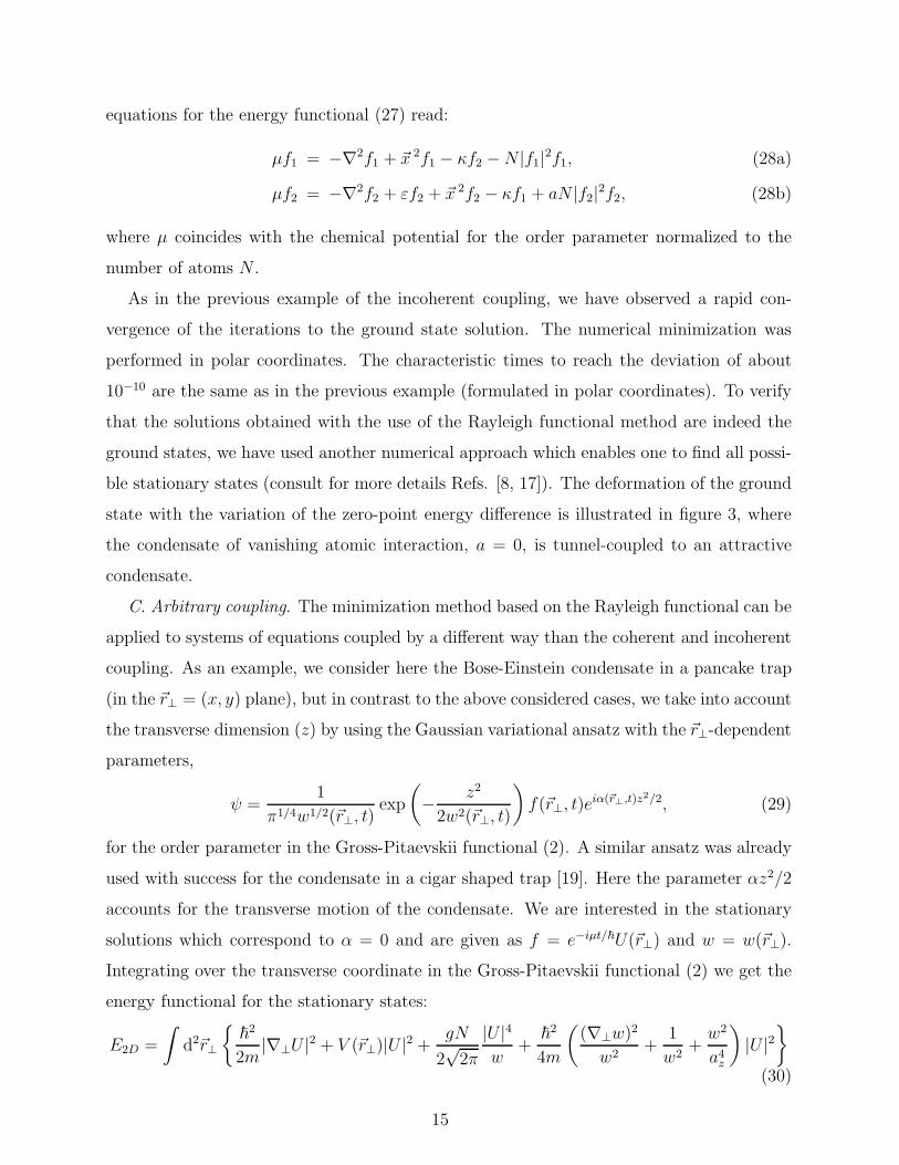
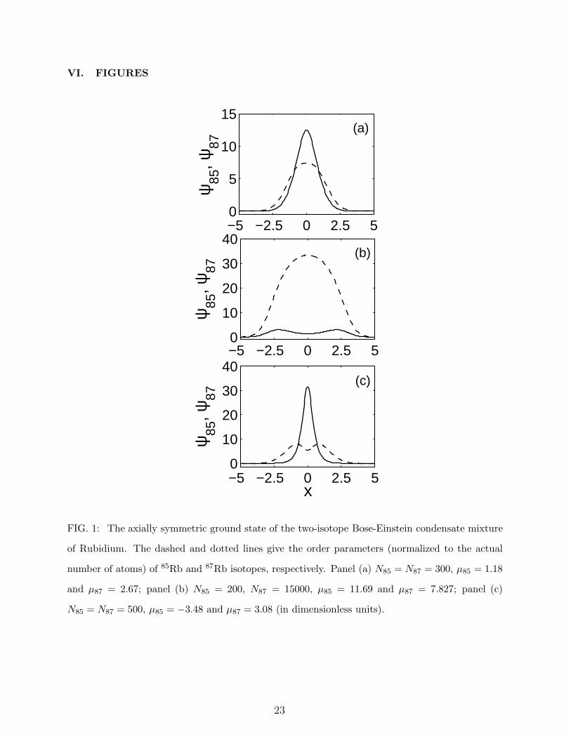
A nontrivial feature of the two-species condensate is that the ground state suffers from

the symmetry breaking transformation, if for instance, for a fixed number of atoms of the

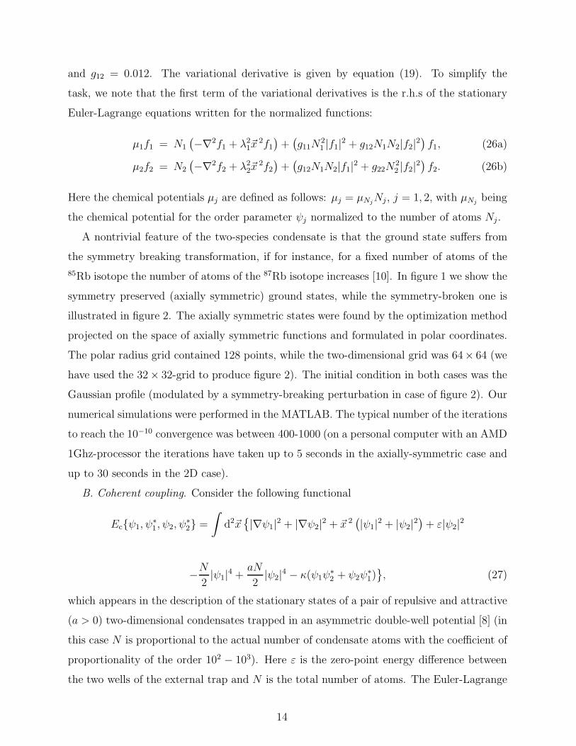
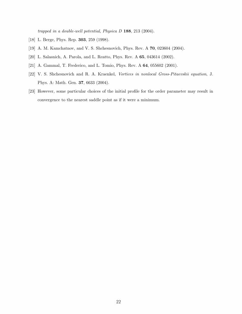
85Rb isotope the number of atoms of the 87Rb isotope increases [10]. In figure 1 we show the

symmetry preserved (axially symmetric) ground states, while the symmetry-broken one is

illustrated in figure 2. The axially symmetric states were found by the optimization method

projected on the space of axially symmetric functions and formulated in polar coordinates.

The polar radius grid contained 128 points, while the two-dimensional grid was 64× 64 (we

have used the 32× 32-grid to produce figure 2). The initial condition in both cases was the

Gaussian profile (modulated by a symmetry-breaking perturbation in case of figure 2). Our

numerical simulations were performed in the MATLAB. The typical number of the iterations

to reach the 10−10 convergence was between 400-1000 (on a personal computer with an AMD

1Ghz-processor the iterations have taken up to 5 seconds in the axially-symmetric case and

up to 30 seconds in the 2D case).

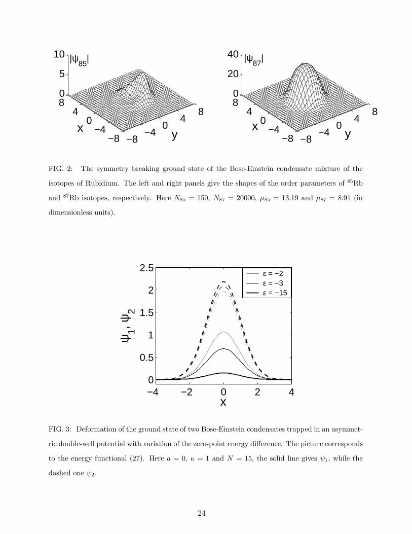
B. Coherent coupling. Consider the following functional

Ecψ1, ψ∗1, ψ2, ψ

∗2 =

∫

d2~x

|∇ψ1|2 + |∇ψ2|2 + ~x 2(

|ψ1|2 + |ψ2|2)

+ ε|ψ2|2

−N2|ψ1|4 +

aN

2|ψ2|4 − κ(ψ1ψ

∗2 + ψ2ψ

∗1)

, (27)

which appears in the description of the stationary states of a pair of repulsive and attractive

(a > 0) two-dimensional condensates trapped in an asymmetric double-well potential [8] (in

this case N is proportional to the actual number of condensate atoms with the coefficient of

proportionality of the order 102 − 103). Here ε is the zero-point energy difference between

the two wells of the external trap and N is the total number of atoms. The Euler-Lagrange

14

equations for the energy functional (27) read:

µf1 = −∇2f1 + ~x 2f1 − κf2 −N |f1|2f1, (28a)

µf2 = −∇2f2 + εf2 + ~x 2f2 − κf1 + aN |f2|2f2, (28b)

where µ coincides with the chemical potential for the order parameter normalized to the

number of atoms N .

As in the previous example of the incoherent coupling, we have observed a rapid con-

vergence of the iterations to the ground state solution. The numerical minimization was

performed in polar coordinates. The characteristic times to reach the deviation of about

10−10 are the same as in the previous example (formulated in polar coordinates). To verify

that the solutions obtained with the use of the Rayleigh functional method are indeed the

ground states, we have used another numerical approach which enables one to find all possi-

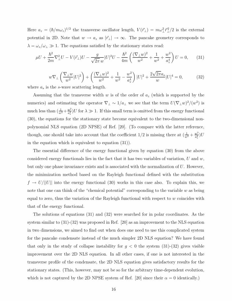
ble stationary states (consult for more details Refs. [8, 17]). The deformation of the ground

state with the variation of the zero-point energy difference is illustrated in figure 3, where

the condensate of vanishing atomic interaction, a = 0, is tunnel-coupled to an attractive

condensate.

C. Arbitrary coupling. The minimization method based on the Rayleigh functional can be

applied to systems of equations coupled by a different way than the coherent and incoherent

coupling. As an example, we consider here the Bose-Einstein condensate in a pancake trap

(in the ~r⊥ = (x, y) plane), but in contrast to the above considered cases, we take into account

the transverse dimension (z) by using the Gaussian variational ansatz with the ~r⊥-dependent

parameters,

ψ =1

π1/4w1/2(~r⊥, t)exp

(

− z2

2w2(~r⊥, t)

)

f(~r⊥, t)eiα(~r⊥,t)z

2/2, (29)

for the order parameter in the Gross-Pitaevskii functional (2). A similar ansatz was already

used with success for the condensate in a cigar shaped trap [19]. Here the parameter αz2/2

accounts for the transverse motion of the condensate. We are interested in the stationary

solutions which correspond to α = 0 and are given as f = e−iµt/~U(~r⊥) and w = w(~r⊥).

Integrating over the transverse coordinate in the Gross-Pitaevskii functional (2) we get the

energy functional for the stationary states:

E2D =

∫

d2~r⊥

~2

2m|∇⊥U |2 + V (~r⊥)|U |2 +

gN

2√

2π

|U |4w

+~

2

4m

(

(∇⊥w)2

w2+

1

w2+w2

a4z

)

|U |2

(30)

15

Here az = (~/mωz)1/2 the transverse oscillator length, V (~r⊥) = mω2

⊥~r2⊥/2 is the external

potential in 2D. Note that w → az as |~r⊥| → ∞. The pancake geometry corresponds to

λ = ωz/ω⊥ ≫ 1. The equations satisfied by the stationary states read:

µU +~

2

2m∇2

⊥U − V (~r⊥)U − g√2π w

|U |2U − ~2

4m

(

(∇⊥w)2

w2+

1

w2+w2

a4z

)

U = 0, (31)

w∇⊥

(∇⊥w

w2|U |2

)

+

(

(∇⊥w)2

w2+

1

w2− w2

a4z

)

|U |2 +2√

2πasw

|U |4 = 0, (32)

where as is the s-wave scattering length.

Assuming that the transverse width w is of the order of az (which is supported by the

numerics) and estimating the operator ∇⊥ ∼ 1/a⊥ we see that the term U(∇⊥w)2/(w2) is

much less than ( 1w2 +w2

a4z)U for λ≫ 1. If this small term is omitted from the energy functional

(30), the equations for the stationary state become equivalent to the two-dimensional non-

polynomial NLS equation (2D NPSE) of Ref. [20]. (To compare with the latter reference,

though, one should take into account that the coefficient 1/2 is missing there at ( 1w2 + w2

a4z)U

in the equation which is equivalent to equation (31)).

The essential difference of the energy functional given by equation (30) from the above

considered energy functionals lies in the fact that it has two variables of variation, U and w,

but only one phase invariance exists and is associated with the normalization of U . However,

the minimization method based on the Rayleigh functional defined with the substitution

f → U/||U || into the energy functional (30) works in this case also. To explain this, we

note that one can think of the “chemical potential” corresponding to the variable w as being

equal to zero, thus the variation of the Rayleigh functional with respect to w coincides with

that of the energy functional.

The solutions of equations (31) and (32) were searched for in polar coordinates. As the

system similar to (31)-(32) was proposed in Ref. [20] as an improvement to the NLS equation

in two dimensions, we aimed to find out when does one need to use this complicated system

for the pancake condensate instead of the much simpler 2D NLS equation? We have found

that only in the study of collapse instability for g < 0 the system (31)-(32) gives visible

improvement over the 2D NLS equation. In all other cases, if one is not interested in the

transverse profile of the condensate, the 2D NLS equation gives satisfactory results for the

stationary states. (This, however, may not be so for the arbitrary time-dependent evolution,

which is not captured by the 2D NPSE system of Ref. [20] since their α = 0 identically.)

16

To illustrate this, in fig. 4 we give the relative difference between the solutions U(r⊥)

of the system (31)-(32) and the corresponding 2D NLS equation for several values of the

nonlinearity strength in the case of repulsive condensate (g > 0). The solution is given in

the units of 1/a⊥, a⊥ = (~/mω⊥)1/2, the radius r⊥ in terms of a⊥, and µ in terms of ~ω⊥/2.

The dimensionless nonlinearity strength is defined as G = 4√

2πas/az. We have set λ = 100

which corresponds to the ratio a⊥/az = 10. The transverse width w, given in terms of az, is

shown in fig. 5. The maximal difference from az is of the order of 10%.

Though in the case of attractive condensate the relative difference between the solutions

of the system (31)-(32) and the 2D NLS equation is also small, the critical value for collapse

differs noticeably. The critical value of the number of atoms is defined by ∂µ/∂N = ∞, i. e.

it is the endpoint coordinate of the curves in fig. 6. The system (31)-(32) is an improvement

over the NLS equation in this case, since the critical value differs by only 2% for λ ≥ 20

from the actual value of the 3D condensate obtained in Ref. [21]. The 2D NLS value is

achieved as the asymptotic limit when λ→ ∞.

We have argued that the minimization based on the Rayleigh functional is always suitable

for obtaining the ground state solutions. However, the possibility of obtaining excited states

was not excluded at all. In contrast to the linear eigenvalue problem of section II in the

nonlinear case there is no general approach which would guarantee computation of all excited

states, though there are some advances in this direction [5]. However, a proper selection of

the initial condition for minimization may lead to convergence to the “nearest” excited state.

We illustrate this on the multi-vortex solutions of a nonlocal Gross-Pitaevskii equation,

which in dimensionless form, in the frame of reference rotating with the frequency Ω, reads

(see the details in Ref. [22])

i∂tΨ = −∇2Ψ + ~x 2Ψ − ΩLzΨ + gΨ

∫

d~x ′2K(|~x − ~x ′|)|Ψ(~x ′)|2. (33)

Here K = 12πa2

K0

(

ra

)

, K0(z) is the Macdonald function, a is the effective range of atomic

interaction, Lz is the angular momentum projection on the z-axis: Lz = −i(x∂y − y∂x) =

−i∂θ, where θ is the polar angle, and Ω is the rotation frequency. For simplicity, we consider

the periodic boundary conditions along the z-axis, Ψ(z + d) = Ψ(z).

We searched for new non-axial vortex solutions, involving combinations of vortices and

antivortices, which represent the excited states of the system, since in the nonlocal GP equa-

tion (33), similar as the in local one, the stationary vortex solutions involving combinations

17

of vortices and antivortices are never the energy minimizers. The energy is minimized by

Tkachenko lattices comprised of vortices only [22].

In figures 7 and 8 we give two examples of excited states comprised of vortex and anti-

vortex combinations (the right panel) and the respective energy minimizers (the left panel).

These solutions were found by using the initial conditions with the phase resembling that of

the multi-vortex solution in quest.

IV. RAYLEIGH FUNCTIONAL IN THE ANALYTICAL APPROACH

The ground state solution of a nonlinear partial differential equation is degenerate if fixing

the l2-norm does not select a unique chemical potential. In the critical case, when there are

infinitely many stationary points with equal energy and the same l2-norm, the nonlinear

optimization method based on the Rayleigh functional may not converge at all.

To clarify this let us consider the critical NLS equation. The ground state of the focusing

critical NLS equation is infinitely degenerate. It is well-known (see, for instance, Refs.

[2, 18]) that the two-dimensional critical NLS equation has a family of soliton solutions

having the same l2-norm ||ψ||2 ≈ 11.69 and a specific member ψ = eitR(~x ) satisfying the

stationary equation

∇2R +R3 −R = 0 (34)

is called the Townes soliton. The stationary NLS equation

µψ + ∇2ψ + |ψ|2ψ = 0 (35)

admits the scale invariance given by ψ(~x ) → kψ(k~x ) and µ → k2µ. Easy to see that,

in two spatial dimensions, the scale invariance preserves the l2-norm of the solution, while

the energy of the stationary solution is exactly zero (see below). This is precisely why

one cannot obtain the Townes soliton by the nonlinear optimization method based on the

Rayleigh functional – the method fails to converge.

This drawback of the Rayleigh functional in the numerical approach turns out into an

advantage for the analytical analysis. Indeed, for the critical NLS equation it immediately

leads to the well-known identity [18]

−µ∫

d2~x |ψ|2 =

∫

d2~x |∇ψ|2 =1

2

∫

d2~x |ψ|4, (36)

18

which is satisfied by any stationary solution. Let us show this. First of all, it is easy

to see that the energy functional of the NLS equation E =∫

d2~x (|∇ψ|2 − |ψ|4/2) has a

scale invariance property: E → k2E for ψ(t, ~x ) → kψ(k2t, k~x ). The invariance property is

transferred to the Rayleigh functional: R → k2R. Differentiation of the latter with respect

to the scale invariance factor k gives R = 0 at the stationary point. Hence, the second

equality in equation (36) follows. The first equality is derived by integrating the stationary

equation multiplied by ψ∗ and using the already proven equality.

In the above derivation we have explicitly related identity (36) to the scale invariance

property. The scale invariance is responsible for the exact balance of energies in any sta-

tionary solution of the critical NLS equation: the kinetic energy is balanced by the energy

due to the self-interaction.

The identity (36) is well-known. However, the point we try to make here that its relation

to the critical scaling makes such an identity universal, i.e. it appears in connection to any

nonlinear equation for which the energy functional has a scaling invariance for a family of

solutions with the same l2-norm. Such is also the one-dimensional critical NLS equation (in

the stationary form)

µψ +d2ψ

dx2+ |ψ|4ψ = 0. (37)

In this case the scale invariance is ψ(x) →√kψ(kx) and µ → k2µ leads to the energy scaling

E → k2E, with E =∫

dx(|dψ/dx|2 − |ψ|6/3), while the l2-norm N =∫

dx|ψ|2 remains

unchanged. Hence the Rayleigh functional scales as follows R → k2R and, by repetition of

the above arguments, we get a similar identity satisfied by the family of stationary solutions:

−µ∫

dx|ψ|2 =

∫

dx

∣

∣

∣

∣

dψ

dx

∣

∣

∣

∣

2

=1

3

∫

dx|ψ|6. (38)

Note that one cannot use the energy functional in the above argument: the stationary

solution is not an extremal of the energy functional. Using the Lagrange modified functional

will not help either due to the explicit appearance of µ. The use of the Rayleigh functional

is indispensable in this short derivation.

V. CONCLUSION

Numerical search for stationary points of nonlinear partial differential equations is a

difficult problem. To tackle such a problem one is left to try various methods and choose

19

the one which gives a better performance and accuracy. In this paper we have proposed a

new numerical method, the nonlinear optimization method based on the Rayleigh functional.

This method is a natural generalization of Poincare’s minmax principle for linear equations,

formulated with the use of the Rayleigh quotient.

It turns out that the imaginary time relaxation method, a widely used method in the

computational physics, is just a special case of nonlinear optimization based on the Rayleigh

functional. We have used the gradient scheme for minimization of the Rayleigh functional,

but this is not essential: one can use the minimization schemes which do not require use of

the gradient.

The simplicity of the Rayleigh functional and its universality for nonlinear equations is

one of the advantages of the method. Moreover, the method can distinguish between the

local minima and saddle points, since the second variation of the Rayleigh functional is

equal to the second variation of the Lagrange modified energy functional, if the latter is

evaluated in the space of normalized functions. The Rayleigh functional takes care of the

normalization constraint of the stationary solution. Other constraints, however, have to be

treated in the usual way.

There are, however, some exceptional cases when the nonlinear optimization based on

the Rayleigh functional may fail. The principal cause of the failure is the infinite degeneracy

of the ground state solution. Still, a failure in the numerics is partially compensated by the

fact that the very degeneracy allows one to get an important analytical insight relating the

scale invariance and an identity satisfied by the stationary solutions in the critical case.

Acknowledgements

This work was supported by CNPq and FAPEAL of Brazil. The initial part of this work

was done during the author’s visit of the Instituto de Fisica Teorica, Universidade Estadual

Paulista, in Sao Paulo, Brazil, which was supported by the FAPESP. We are grateful to

Jianke Yang for helpful suggestions.

[1] L. Pitaevskii and S. Stringari, Bose-Einstein Condensation (Clarendon Press, Oxford, 2003).

20

[2] C. Sulem and P. L. Sulem, The nonlinear Schrodinger equation: self-focusing and wave-

collapse, Applied Mathematical Sciences, 139, Springer-Verlag, 1999.

[3] R. Fletcher, Practical Methods of Optimization (2nd. Edition, Jonh Wiley & Sons, New York,

1987).

[4] J. Nocedal, Theory of Algorithms for Unconstrained Optimization, Acta Numerica 199, 242

(1992).

[5] J. J. Garcia-Ripoll and V. M. Perez-Garcia, Optimizing Schrodinger functionals using Sobolev

gradients: Applications to quantum mechanics and nonlinear optics, SIAM J. Sci. Comput.

23, 1315 (2001).

[6] L. D. Landau and E. M. Lifshitz, Quantum Mechanics (3rd edition, Pergamon Press, Oxford,

1987).

[7] L. C. Crasovan et al, Phys. Rev. A 66, 036612 (2002).

[8] V. S. Shchesnovich, S. B. Cavalcanti, Stable stationary states in two tunnel-coupled two-

dimensional condensates with the scattering lengths of opposite signs, to appear in J. Phys. A:

Math. Gen. (2005).

[9] V. S. Shchesnovich, S. B. Cavalcanti, and R. A. Kraenkel, Solitons in tunnel-coupled repulsive

and attractive condensates, Phys. Rev. A 69, 033609 (2004).

[10] V. S. Shchesnovich, A. M. Kamchatnov, and R. A. Kraenkel, Mixed-isotope Bose-Einstein

condensates in rubidium, Phys. Rev. A 69, 033601 (2004).

[11] J. Barzilai and J. M. Borwein, Two-point step gradient methods, IMA J. Numer. Analys. 8,

141 (1988).

[12] M. Raydan, The Barzilai and Borwein gradient method for the large scale unconstrained min-

imization problem, SIAM J. Optim. 7, 26 (1997).

[13] R. Fletcher, On the Barzilai-Borwein method, Research Report Department of Mathematics,

University of Dundee, 2001.

[14] B. Fornberg, A Practical Guide to Pseudospectral Methods, (Cambridge, UK: Cambridge Uni-

versity Press) 1996.

[15] J. P. Boyd, Chebyshev and Fourier Spectral Methods, (Second ed., New York: DOVER Pub-

lications Inc.) 2000.

[16] L. N. Trefethen, Spectral Methods in Matlab, (Philadelphia: SIAM) 2000.

[17] V. S. Shchesnovich, B. A. Malomed, and R. A. Kraenkel, Solitons in Bose-Einstein condensates

21

trapped in a double-well potential, Physica D 188, 213 (2004).

[18] L. Berge, Phys. Rep. 303, 259 (1998).

[19] A. M. Kamchatnov, and V. S. Shchesnovich, Phys. Rev. A 70, 023604 (2004).

[20] L. Salasnich, A. Parola, and L. Reatto, Phys. Rev. A 65, 043614 (2002).

[21] A. Gammal, T. Frederico, and L. Tomio, Phys. Rev. A 64, 055602 (2001).

[22] V. S. Shchesnovich and R. A. Kraenkel, Vortices in nonlocal Gross-Pitaevskii equation, J.

Phys. A: Math. Gen. 37, 6633 (2004).

[23] However, some particular choices of the initial profile for the order parameter may result in

convergence to the nearest saddle point as if it were a minimum.

22

VI. FIGURES

−5 −2.5 0 2.5 50

5

10

15

ψ85

, ψ87

−5 −2.5 0 2.5 50

10

20

30

40

ψ85

, ψ87

−5 −2.5 0 2.5 50

10

20

30

40

x

ψ85

, ψ87

(a)

(b)

(c)

FIG. 1: The axially symmetric ground state of the two-isotope Bose-Einstein condensate mixture

of Rubidium. The dashed and dotted lines give the order parameters (normalized to the actual

number of atoms) of 85Rb and 87Rb isotopes, respectively. Panel (a) N85 = N87 = 300, µ85 = 1.18

and µ87 = 2.67; panel (b) N85 = 200, N87 = 15000, µ85 = 11.69 and µ87 = 7.827; panel (c)

N85 = N87 = 500, µ85 = −3.48 and µ87 = 3.08 (in dimensionless units).

23

−8−4

04

8

−8−4

04

80

5

10

−8−4

04

8

−8−4

04

80

20

40|ψ85

| |ψ87

|

x y x

y

FIG. 2: The symmetry breaking ground state of the Bose-Einstein condensate mixture of the

isotopes of Rubidium. The left and right panels give the shapes of the order parameters of 85Rb

and 87Rb isotopes, respectively. Here N85 = 150, N87 = 20000, µ85 = 13.19 and µ87 = 8.91 (in

dimensionless units).

−4 −2 0 2 40

0.5

1

1.5

2

2.5

x

ψ1, ψ

2

ε = −2ε = −3ε = −15

FIG. 3: Deformation of the ground state of two Bose-Einstein condensates trapped in an asymmet-

ric double-well potential with variation of the zero-point energy difference. The picture corresponds

to the energy functional (27). Here a = 0, κ = 1 and N = 15, the solid line gives ψ1, while the

dashed one ψ2.

24

0 2 4 6 8 10 12−2

−1

0

1

2

3

4

r⊥

δU/U

GN =10GN = 100GN = 1000GN = 5000GN = 10000

×10−3

FIG. 4: The relative difference between the solutions of the 2D NLS equation and the system

(31)-(32). Here λ = 100.

0 2 4 6 8 101

1.02

1.04

1.06

1.08

1.1

w

r⊥

GN = 10GN = 100GN = 1000GN = 5000GN = 10000

FIG. 5: The transverse width of the condensate given by the system (31)-(32). Here λ = 100.

25

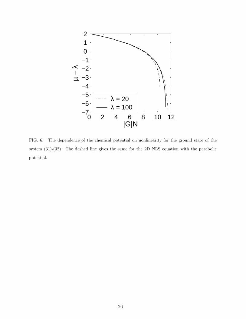
0 2 4 6 8 10 12−7−6−5−4−3−2−10 1 2

|G|N

µ −

λ

λ = 20λ = 100

FIG. 6: The dependence of the chemical potential on nonlinearity for the ground state of the

system (31)-(32). The dashed line gives the same for the 2D NLS equation with the parabolic

potential.

26

FIG. 7: The stationary vortex solutions for a = 0.052, g = 104 and Ω = 0.38. The left panel

shows the 3-vortex solution and the right one – the 5-vortex solution comprised of 4 vortices and

1 antivortex (in the center).

27

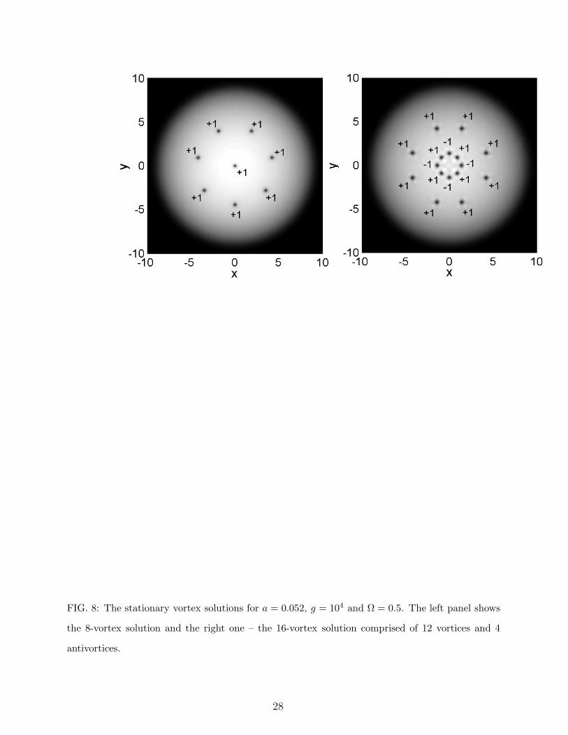
FIG. 8: The stationary vortex solutions for a = 0.052, g = 104 and Ω = 0.5. The left panel shows

the 8-vortex solution and the right one – the 16-vortex solution comprised of 12 vortices and 4

antivortices.

28